
Band-Optimized Bidirectional LSTM Deep Learning Model for Bathymetry Inversion

College of Information, Shanghai Ocean University, No. 999 Hucheng Ring Road, Shanghai 201306, China
*
Author to whom correspondence should be addressed.
Remote Sens. 2023, 15(14), 3472; https://doi.org/10.3390/rs15143472
Submission received: 16 May 2023
/
Revised: 5 July 2023
/
Accepted: 6 July 2023
/
Published: 10 July 2023
(This article belongs to the Special Issue Multi-Source Data Observations of Shallow Water Area — Methods, Ecosystem, Geomorphology and Environment)
Abstract
:Shallow water bathymetry is of great significance in understanding, managing, and protecting coastal ecological environments. Many studies have shown that both empirical models and deep learning models can achieve promising results from satellite imagery bathymetry inversion. However, the spectral information available today in multispectral or/and hyperspectral satellite images has not been explored thoroughly in many models. The Band-optimized Bidirectional Long Short-Term Memory (BoBiLSTM) model proposed in this paper feeds only the optimized bands and band ratios to the deep learning model, and a series of experiments were conducted in the shallow waters of Molokai Island, Hawaii, using hyperspectral satellite imagery (PRISMA) and multispectral satellite imagery (Sentinel-2) with ICESat-2 data and multibeam scan data as training data, respectively. The experimental results of the BoBiLSTM model demonstrate its robustness over other compared models. For example, using PRISMA data as the source image, the BoBiLSTM model achieves RMSE values of 0.82 m (using ICESat-2 as the training data) and 1.43 m (using multibeam as the training data), respectively, and because of using the bidirectional strategy, the inverted bathymetry reaches as far as a depth of 25 m. More importantly, the BoBiLSTM model does not overfit the data in general, which is one of its advantages over many other deep learning models. Unlike other deep learning models, which require a large amount of training data and all available bands as the inputs, the BoBiLSTM model can perform very well using equivalently less training data and a handful of bands and band ratios. With ICESat-2 data becoming commonly available and covering many shallow water regions around the world, the proposed BoBiLSTM model holds potential for bathymetry inversion for any region around the world where satellite images and ICESat-2 data are available.
1. Introduction
Bathymetry in coastal areas is crucial to seabed landform surveying, environmental construction in coastal zones, the protection of coral reef ecosystems, and ship navigation and transportation [1,2,3,4,5]. Commonly used techniques of bathymetry include the traditional shipborne multibeam sounding surveys and recent Airborne Lidar Bathymetry (ALB) surveys. Shipborne multibeam sounding measurement [6] is affected by draft restrictions, waves, and rocks, making it very dangerous to measure in shallow water [7]. Although ALB can correct some of these defects, the maximum water depth measured is limited by the quality of the water body and the water penetration of laser pulses [8,9,10], and shallow water bathymetric mapping is prohibitively expensive [11,12]. Other bathymetry methods include combining wave kinematics [13], physical wave models based on Gaussian process regression [14], dual-medium stereo photogrammetry [15], and synthetic aperture radar [16] and utilizing monitoring systems such as UAVs [17,18,19] to estimate water depth. With the development of satellite and remote sensing technology, large-scale and high-resolution data can be obtained by using satellite images, which have been widely used in bathymetry [20,21,22,23,24]. Common bathymetry inversion models for satellite-derived bathymetry (SDB) are mainly empirical models such as those described by Lyzenga [25] and Stumpf [26]. Recent studies focus on models which use localized optimization techniques such as graphically weighted regression (GWR) [27] or kriging with an external drift (KED) [28] to improve global optimization models. These models usually use limited bands for bathymetry inversion. For hyperspectral and multispectral images, the water reflectance information could be contained in many bands and it is therefore desirable to utilize all available information for bathymetry inversion.
With the rapid advancement of deep learning in various fields, multi-band bathymetry inversion using neural networks and in situ water depth data has gained popularity as an alternative to traditional empirical methods. Artificial neural network (ANN)-based methods have been shown to effectively invert bathymetry in optical shallow water areas [29] and classify seabed types [30]. However, these methods may suffer from slow convergence speeds and sample dependence. To address these limitations, Liu et al. [31] propose an LABPNN-based shallow water bathymetry model for optical remote sensing images to deal with low-quality and sparse sample data. Neural network models can perform bathymetric estimation to depths of up to 20 m, outperforming optimal band ratio analysis (OBRA) [32]. The performance of bathymetry inversion can be further improved by using models such as the Adjacent Pixels Multilayer Perceptron Model (APMLP) to account for the influence of the seafloor matrix and Inherent Optical Properties (IOP) [33]. In recent studies [34], complementary approaches based on color information and wave kinematics have been explored to deduce bathymetry in clear seawater and turbid coastal areas using deep learning models. Additionally, convolutional neural networks (CNNs) combined with structure-from-motion (SfM) photogrammetry [35] or leveraging local spatial correlations between pixels [36] can also be used for bathymetric inversion. High-resolution bathymetry maps can be generated using deep convolutional neural network SegNet and Sentinel-2 images [37]. In summary, remote sensing satellite images combined with deep learning models offer improved accuracy for bathymetry inversion in general.
When deep learning models are applied to bathymetry inversion, they face two main challenges. Firstly, they require a large amount of training data, which are difficult to collect in shallow water areas due to constraints in time, space, and cost. Fortunately, the recent launch of the Ice, Cloud, and Land Elevation Satellite-2 (ICESat-2) [38,39] has provided highly accurate bathymetry reference depth information for near-shore water bathymetry [40,41]. The second challenge of deep learning models is determining which spectral bands or band ratios are significant for deep learning models in inverting bathymetry in multispectral or hyperspectral imagery [42]. Typically, bands such as the blue, green, red, or near-infrared bands are used to retrieve bathymetry from multispectral images [43,44,45,46]. Hyperspectral images can contain many combinations of bands and band ratios for the performance of fitting analysis [47,48,49], or they can accurately and quickly measure shallow bathymetry through image data dimensionality reduction [50]. However, existing methods have primarily focused on specific spectral information and have not thoroughly analyzed the contribution of different bands or band ratios in different images to bathymetry inversion. Research on multi-band selection and band contributions during deep learning processes could potentially enhance bathymetry inversion accuracy and the effectiveness of deep learning applications.
This paper attempts to introduce double-layer Long Short-Term Memory (DLSTM) [51], CNN-LSTM [52], and Bidirectional LSTM (BiLSTM) [53] deep learning models for bathymetry inversion using satellite multispectral and hyperspectral images. Considering that BiLSTM can store bidirectional coding information at the same time, and aiming at the importance of the spectral features of satellite images, a BoBiLSTM (Band-optimized BiLSTM) model is proposed to improve the performance of bathymetry inversion. The BoBiLSTM model uses two algorithms (dual-band selection and multi-band selection) to select the most important bands and band ratios, respectively. The dual-band selection algorithm uses the Stumpf model to select the two optimal bands each time, while the multi-band selection algorithm employs a Gradient Boosting Decision Tree (GBDT) [54] to conduct evaluations for all bands based on their contributions to bathymetry inversion, with only the bands and band ratios with significance to bathymetry inversion retained. The bands and band ratios obtained from above are used as the inputs for the BoBiLSTM model, and the geographic coordinates of the training points are also added to the model as a sequential sequence for training so that it strengthens bidirectional learning of the bathymetric information in the shallow water areas and the relevantly deeper water areas. The experiments were conducted in the shallow water region in the southeast of Molokai Island, the fifth largest island of the Hawaii Archipelago. The main contributions of this paper are as follows: (1) BiLSTM is introduced for the first time for bathymetry inversion; (2) a new strategy of selecting bands and band ratios is proposed to reduce the amount of input data and improve accuracy; (3) the proposed BoBiLSTM model outperforms DLSTM, CNN-LSTM, BiLSTM, and Stumpf models, as demonstrated through of a series of experiments; (4) ICESat-2 data are shown to be a very suitable source of training data for satellite-derived bathymetry.
The research in this paper makes up for the limitation of traditional empirical models that are only applicable to single-band and dual-band selections and provides a better deep learning method for bathymetry inversion from multiple data sources.
2. Materials and Methods
2.1. Analysis Area
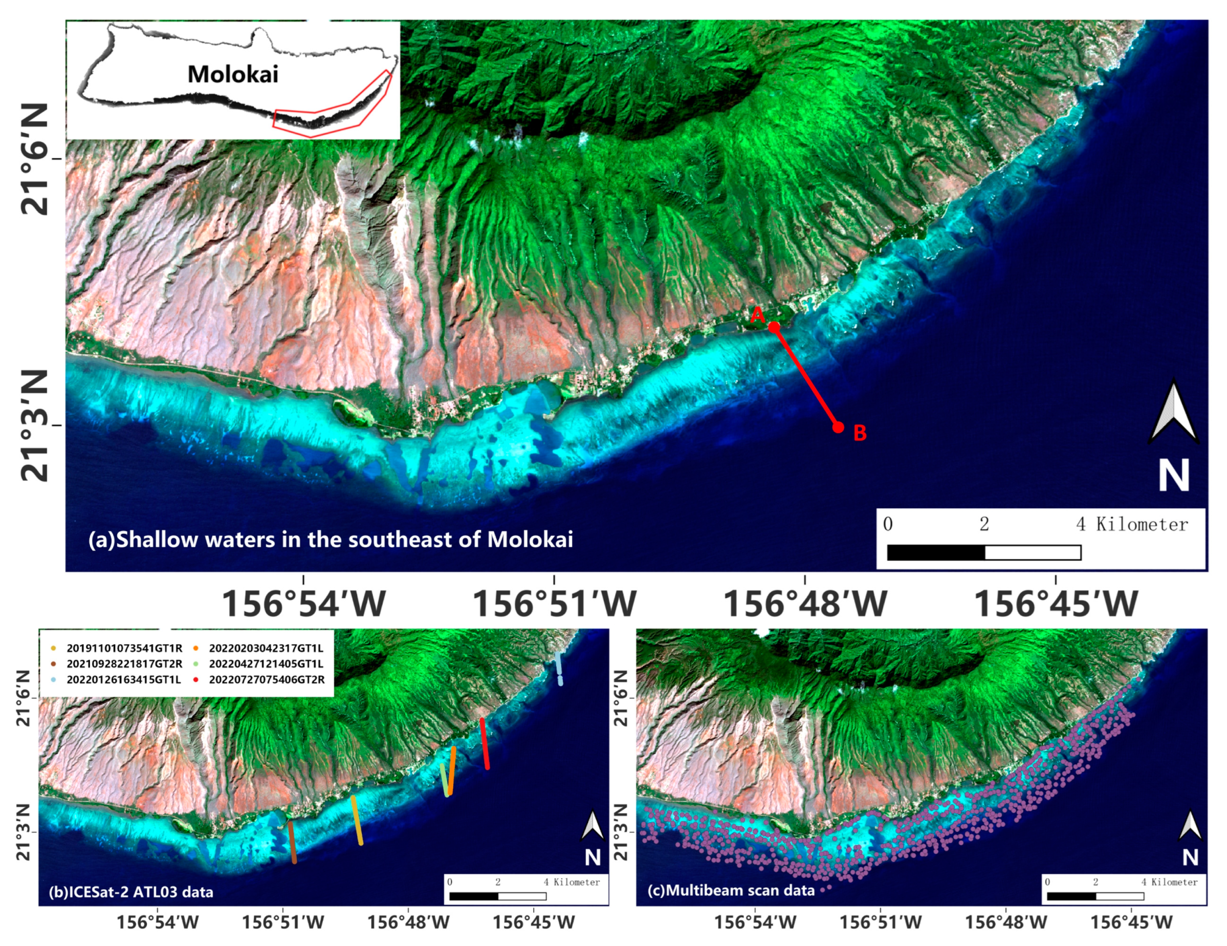
Molokai Island is the fifth largest island of the Hawaii Archipelago, with a length of 62 km from east to west and an average width of 13 km from north to south. It has a natural coastline of 140 km and covers an area of 670 km2. The study area is the shallow waters in the southeast region of Molokai Island. The geographic coordinates extend from 156°44′W to 156°57′W (longitude) and from 21°1′N to 21°7′N (latitude). The water quality in this sea area is relatively clear [3], and the radiation values of optical remote sensing are less influenced by factors commonly seen in other regions. Figure 1a is a satellite image of the study area, which only shows the RGB channels of a Sentinel-2 image.
2.2. Existing Methods
The log-band ratio method of Stumpf et al. for SDB mapping assumes that the area has a uniform bottom and a log-band ratio of water-leaving reflectance that decreases linearly with water depth. In order to compare the effects of different models on bathymetry inversion, we chose the Stumpf model as a typical empirical model to be compared with. The Stumpf model uses the ratio logarithm of two bands to express the relationship between reflectance and in situ water depth:
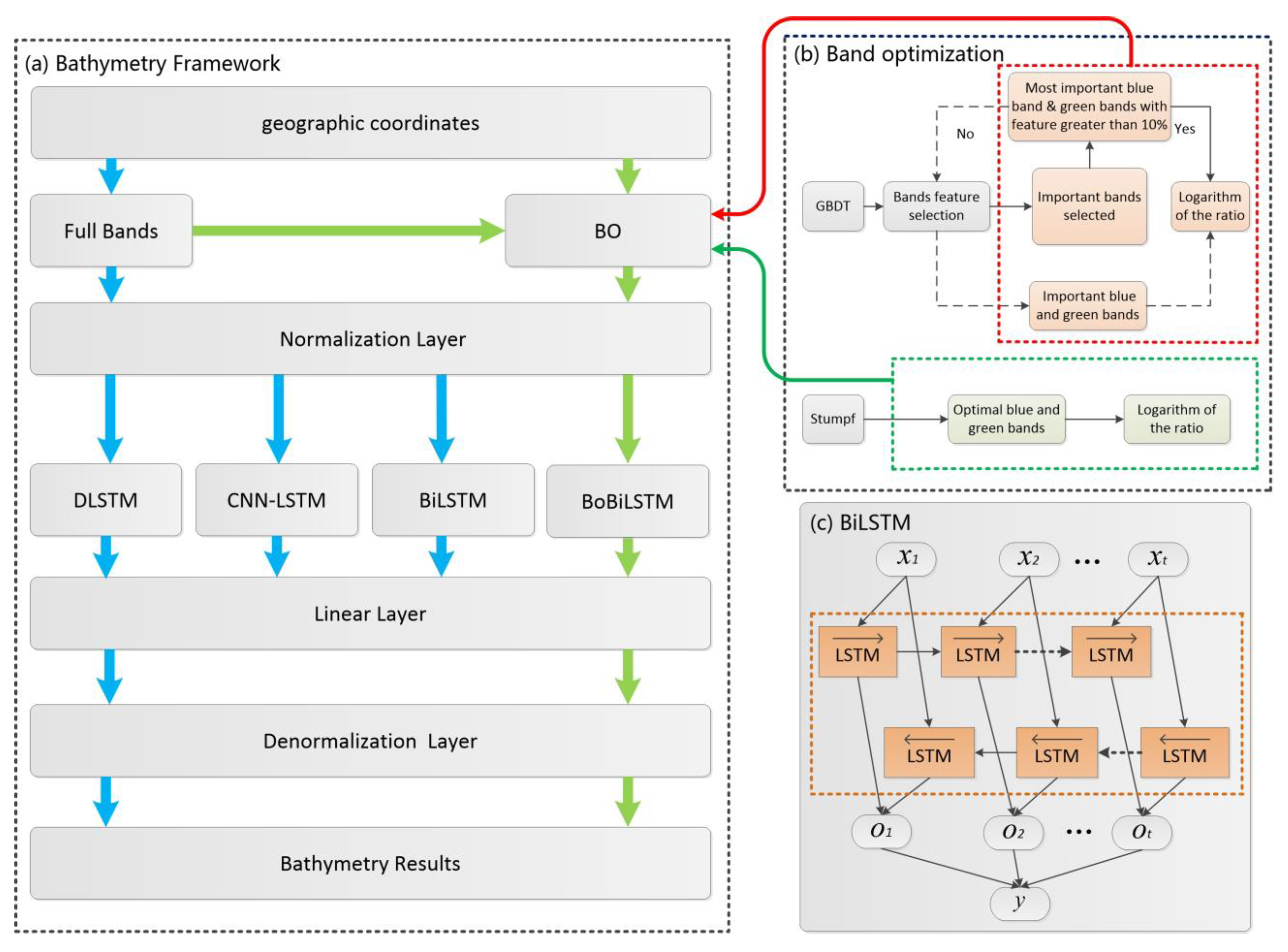
In order to evaluate the performance of the BoBiLSTM model against other deep learning models, DLSTM, CNN-LSTM, and BiLSTM models were chosen for comparison. These models can handle regression, prediction, and classification problems [55,56,57]. However, there are few studies on bathymetry inversion. Therefore, in order to explore whether different deep learning models have good robustness and accuracy in bathymetry inversion, this study attempts to apply these models for SDB. The DLSTM model uses two layers of LSTM neural networks in the same direction, and the BiLSTM model uses two layers of bidirectional LSTM neural networks. The neuron settings of the LSTM layers of these two models are the same. The CNN layer in the CNN-LSTM model uses a one-dimensional convolutional layer. The LSTM layer parameter settings are the same as the second-layer LSTM layer of the DLSTM model. The bathymetry inversion framework of the three models is shown by the blue arrows in Figure 3a. In this study, full bands and geographic coordinates of in situ water depth were used as inputs for these three models. The specific parameter settings are shown in Table 1.
2.3. Datasets
2.3.1. PRISMA—Hyperspectral Satellite Images
The PRISMA hyperspectral satellite is a small hyperspectral imaging satellite that was launched by the Italian Space Agency on 22 March, 2019. It is equipped with a hyperspectral imager (PRISMA HSI) and a medium-resolution panchromatic camera [58]. It has a total of 239 bands, with a spectral range from 400 nm to 2500 nm, and can acquire images with a spatial resolution of 30 m. Of the 239 bands, 66 bands belong to the visible and near-infrared range (VNIR), with the other 173 bands belonging to the short-wave infrared range (SWIR). In order to compare the results of bathymetry retrieved from PRISMA images to the results from multispectral satellite (Sentinel-2) images, only 63 VNIR bands of PRISMA data were selected (bands 1–3 are empty). The PRISMA images used in the experiments were acquired at 21:13 (UTM) on 22 April, 2020, and the study area was cloudless. The main bands and the spectrum ranges of PRISMA images are shown in Table 1. The band information of PRISMA images can be found in the official user instruction document [59].
2.3.2. Sentinel-2—Multispectral Satellite Images
Launched by the European Space Agency in 2015, the Sentinel-2 satellite is one of the most widely used multispectral remote sensing satellites around the world today. The satellite has a total of 13 bands with a spectral range including visible, near-infrared, and short-wave infrared, as well as different spatial resolutions of 10 m, 20 m, and 60 m. Sentinel-2 images are provided by the ESA Copernicus Data Center [60]. In this study, the L2A image product obtained at 21:09 (UTM) on 4 February, 2022, was selected for bathymetry inversion on Molokai Island, and the study area was cloudless. The L2A image has been geo-rectified and radiometrically calibrated. On this basis, SNAP software [61] was used to resample all bands to the spatial resolution of 30 m, and layer stacking in ENVI 5.3 was then used to perform band synthesis to form a TIFF image. The map projection is a WGS84 geographic coordinate system. The band information of Sentinel-2 images can be found in the official user manual [62]. Together with PRISMA’s, Sentinel-2′s bands and their spectrum ranges are shown in Table 2.
2.3.3. ICESat-2 Data—Training Data
The recently launched Ice, Cloud, and Land Elevation Satellite-2 (ICESat-2) mission by NASA, equipped with laser altimetry technology, is designed to accurately measure changes in ice sheets and sea ice, providing valuable insights into their dynamics. Onboard ICESat-2, a cutting-edge laser altimetry system called the Advanced Terrain Laser Altimetry System (ATLAS) is utilized, which employs single-micropulse, photon-counting technology. The ATL03 product contains the geographic ellipsoidal height (WGS84, ITRF2014 reference system), latitude, longitude, and time of each photon event [63]. Challenges arise during the preprocessing of ATL03 data due to weather-related factors such as clouds and rainfall, leading to increased photon noise data and difficulties in accurately extracting continuous underwater photon data. Therefore, the area covered by the ATL03 data selected in this study is cloudless and rainless; six selections along the track direction (depicted by solid lines of different colors in Figure 1b) from the six ATL03 datasets were chosen as training points for bathymetry, as shown in Table 3.
To enhance the accuracy of ICESat-2 data for bathymetry, ICESat-2 postprocessing employs water refraction correction and tidal correction. Previous studies [64,65,66] indicate that the position of underwater photon signals in near-shore bathymetry is influenced by water refraction, with greater displacement in deeper waters. Considering the small pointing angle of the laser pulse, this study only accounts for the displacement of photons in the elevation direction to mitigate the impact of seawater refraction on bathymetry. The data processing procedure is as follows: (1) the density-based spatial clustering algorithm (DBSCAN) [67] is utilized to cluster sea surface photons and sea bottom photons separately from the ATL03 data; (2) the height of clustered sea surface photons is utilized to determine the average sea level height and to calculate the elevation difference between the average sea level and each seabed photon to obtain the depth of the seabed photon before seawater refraction; (3) the incident angle of the laser pulse, the refractive index of atmospheric seawater (1.34116), and the calculated results are employed to derive the displacement value of the seabed photon elevation; (4) subsequently, the tide table [68] of the study area is consulted to determine the tide height of the ICESat-2 trajectory to eliminate the influence of tide effects on in situ water depth; and (5) the corrected seawater depth is finally calculated by manually removing some noise data.
2.3.4. Multibeam Scan Data—Training Data
Bathymetry data in the Molokai Sea were acquired from various multibeam systems and ships, such as SeaBeam classic, SeaBeam 2000, SeaBeam 2112, Hydrosweep, and LIDAR [69]. These acquired multibeam scan data were edited using different software tools, such as MB-System, SABER, Caris, and Fledermaus. Meshing of the bathymetry components was carried out using MB-System and the General Mapping Tools (GMT) open-source software package [70]. Subsequently, multibeam bathymetric composite data with a spatial resolution of 5 m were generated.
After processing the sampling data, a total of 751 training points were carefully chosen in the study area, including the coordinates of the training points and the corresponding measured water depth values [71]; the geographical distribution of training points was kept relatively uniform, as depicted in Figure 1c.
2.3.5. Independent Reference Bathymetry Map—Validation Data
To independently validate the proposed bathymetry inversion models, an independent bathymetric dataset developed by the Global Airborne Observatory (GAO) team at the Center for Global Discovery and Conservation Science at Arizona State University was utilized [72,73]. This independent bathymetry map was generated from high-resolution benthic depth data obtained from airborne imaging spectroscopy conducted by the GAO in January 2019 and January 2020. The independent bathymetric map has an impressive spatial resolution of 2 m, and it was compared with the geographic coordinates of the satellite images (ICESat-2) and multibeam scan data for overlap analysis. In the following sections, this independent bathymetry map is called the reference bathymetry map.
2.4. BoBiLSTM Model
The BoBiLSTM model is a band-optimized deep learning method which can filter full-band data and then select the band and band ratio that contribute the most to the water depth, using these as a new input to train the BiLSTM model so as to realize the model’s ability to invert the water depth. The detailed algorithm, frame structure, and parameter settings are introduced as follows.
2.4.1. BiLSTM
LSTM, which stands for Long Short-Term Memory, is a type of recurrent neural network (RNN) introduced in 1997 [74]. LSTM is a form of Gated Recurrent Neural Network (GRNN). The defining characteristic of LSTM is its ability to retain information over long sequences, allowing for future cell processing. LSTM networks are designed to store and manage information in a way that enables them to capture long-term dependencies, making them well suited for tasks that require the modeling of sequential data.
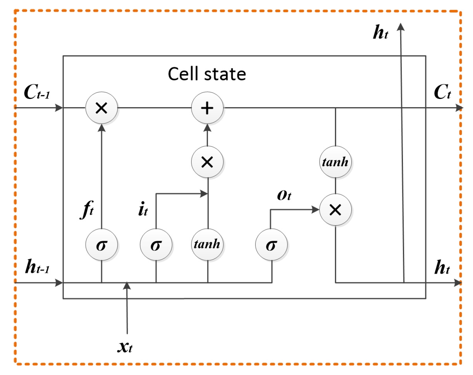
BiLSTM is an extension of LSTM and BRNN [75], where the same sequence is input into two separate LSTM networks, one in the forward direction and the other in the backward direction. The hidden layers of these two networks are then linked together to the output layer for prediction. BiLSTM can encode information from both directions simultaneously, combining the states of the two sets of hidden layers. This allows BiLSTM to capture bidirectional dependencies in sequential data and time steps without increasing the size of the data. BiLSTM is commonly used in applications such as text feature extraction, speech recognition, machine translation, fault prediction, and load forecasting. This paper proposes BiLSTM as the basic model for bathymetric inversion for the first time. The basic configuration of BiLSTM is shown in Figure 3c, and the LSTM unit of its internal structure (shown in Figure 2) is expressed by a series of equations:
where , , and are the state gates at the current point in time , denoting the forget gate, input gate, and output gate, respectively. Their values are between 0 and 1. denotes the output from the previous LSTM unit at the previous moment; denotes the output from the current LSTM unit at the current moment; denotes the cell state at the current moment, deciding the update of information by the gating state; and denotes the cell state of the previous LSTM unit at the previous moment, deciding the input of information by the gating state of the forget gate. and represent the weight and bias of gates in different states. Assuming that the output state of the forward LSTM unit at time is , and the output state of the backward LSTM unit at time is , then the features of the two are concatenated and the final output is the output state of BiLSTM at time .
2.4.2. Band Optimization Method
It can be seen from the above BiLSTM equations and framework that the BiLSTM model is complicated. The spectrum range and the number of bands of different satellite images are very different, and the importance of the features of the bands cannot be clearly highlighted due to the differences in data sources. These will cause the model to perform well on the test set when the amount of data is small or the quality of the data is poor, but the entire image is prone to overfitting. Therefore, it is natural to explore ideas related to how to reduce the amount of inputs to BiLSTM and improve the model’s training efficiency. The solution of this study is to use only limited optimized bands to feed the BiLSTM model, and a new model named BoBiLSTM is therefore proposed.
Band optimization (BO) (Figure 3b) performs full-band feature selection using two algorithms: dual-band selection and multi-band selection. The dual-band selection algorithm is used to select the optimal bands and the logarithm of the band ratio from the bathymetric results estimated by the Stumpf model. The multi-band selection algorithm is performed using a GBDT [76,77] to keep only the most important bands among the many bands. The GBDT is based on the boosting algorithm, which is one of the typical machine learning algorithms and can be used to solve problems such as classification, regression, and feature selection [78,79,80]. The GBDT uses an additive model to achieve regression or prediction by continuously fitting the residuals of the training process. The key equation is as follows:
where , , ,..., represent the weight coefficients of each weak classifier. The GBDT undergoes multiple iterations during the selection process, and each iteration produces a weak classifier that is trained in the direction of further reducing the residual compared to the previous iteration. Because the training process uses the negative gradient of the loss function to approximate the residual, this continuously improves the final prediction accuracy of the model.
In this study, multi-band selection is used for the GBDT regression method to conduct bathymetry inversion evaluation on all bands in the training set, with the importance of the band features then calculated and sorted from large to small before the bands are finally selected in sequential order to make the cumulative sum of their feature values reach more than 90%. This process determines the bands that contribute most to bathymetry inversion. From the bands selected above, the green band with a feature value greater than 10% and the blue band with the most important feature are found and the logarithm of their ratio is calculated. If there are no blue–green bands, the most important blue and green bands from all band features are found.
The bands and band ratios obtained through band optimization are used as the inputs for the BoBiLSTM model, and the geographic coordinates of the in situ water depth points are also added to the model as a sequential sequence for training. The BoBiLSTM model can eliminate bands that contribute less to bathymetry inversion for multispectral or hyperspectral images and retain important bands and the blue–green band ratio widely used in bathymetric inversion.
2.4.3. Bathymetry Inversion Framework
The green arrow in Figure 3a shows the framework of the proposed BoBiLSTM model. Its basic unit consists of a band optimization (BO) layer, a normalization layer, a BiLSTM layer, a linear layer, and a denormalization layer. In order to prevent the model from overfitting, the BoBiLSTM model (128 neurons) adds a dropout layer (set to 0.5) [81] and an activation function (tan h). The loss function used by the model is MSE, and the optimizer is Adam [82].
The normalization layer is used to rescale the band values between 0 and 1 so that the feature values of different dimensions have a certain comparability, thereby improving the accuracy of model training and speeding up the convergence rate of the model in operation. Since bathymetry inversion is ultimately a regression problem, a linear layer is added to the model. When the training set samples are sufficient and of high quality, the water depth range on the training set is infinitely close to the water depth range of the entire prediction area. Under this assumption, the denormalization layer is set up, and the previous normalization parameters of the training set are used to denormalize the water depth values of the predicted data points.
2.5. Evaluation Method
In order to evaluate the accuracy and performance of the Stumpf model and the DLSTM, CNN-LSTM, BiLSTM, and BoBiLSTM deep learning models for SDB, two kinds of satellite image data (hyperspectral PRISMA data and multispectral Sentinel-2 data) and two kinds of bathymetric training data (ICESat-2 data and multibeam scan data, respectively) were used. Each image is combined with two bathymetric data sources. The accuracy assessment was conducted through the calculation of R2 and RMSE for each experiment.
3. Results
3.1. Bathymetry Inversion Using ICESat-2 Data
ICESat-2 data were first corrected due to seawater refraction and tidal correction to obtain accurate training data for bathymetry inversion. To study the ability of the deep learning model to invert water depth, three ATL03 strips (20210928GT2R, 20220203GT1L, and 20220427GT1L) were used as the test set to verify the sounding effect, and the remaining three ATL03 (20191101GT1R, 20220126GT1L, and 20220727GT2R) strips were used as the training set. The data ratio of the training points to the test points is 2542:1600 (a ratio of about 3:2). Finally, bathymetry inversion was performed on PRISMA and Sentinel-2 images for the entire study area.
3.1.1. Bathymetry of ICESat-2 Data
Table 4 lists the minimum water depth and maximum water depth of six ICESat-2 strips in the study area before and after seawater refraction and tidal correction, as well as the reference depth [72,73]. Compared to the reference depth, depth information derived from ICESat-2 is quite close to the reference, except for the 20220126GT1L strip which had a deviation of 4.33 m (for this reason, 20220126GT1L is considered as a validation dataset). The difference between before and after seawater refraction and tidal correction is significant, and proper seawater refraction and tidal correction to the original ICESat-2 data is therefore critical when ICESat-2 is used for bathymetry inversion purpose.
3.1.2. Bathymetry Inversion Using ICESat-2 Data
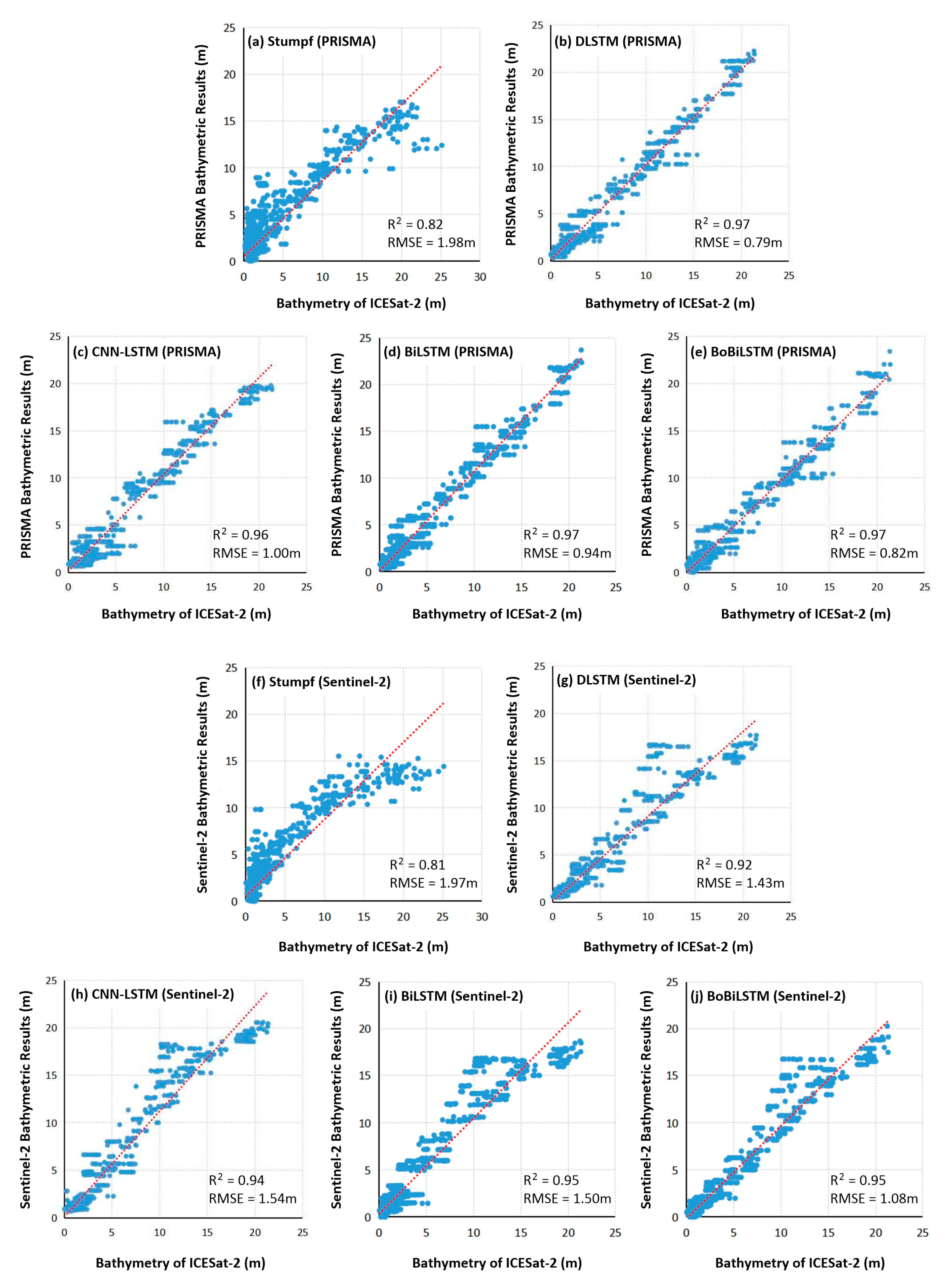
Five models were used for bathymetry inversion for PRISMA and Sentinel-2 images, namely the Stumpf model, DLSTM model, CNN-LSTM model, BiLSTM model, and BoBiLSTM model (shown in Table 5). For PRISMA images, the most commonly used combination of bands selected by the Stumpf model was the blue–green bands 50 and 54, and the effect of its inversion of water depth was the worst among the five models, with an R2 value of 0.82 and a RMSE value close to 2 m. Compared to the Stumpf model, the DLSTM, BiLSTM, and BoBiLSTM models all had higher correlation, with R2 values of 0.97 and RMSE values of less than 1 m. Between the BiLSTM and BoBiLSTM models, it is not surprising that the BoBiLSTM model beats the BiLSTM model in terms of RMSE values (0.82 m vs. 0.94 m). This was due to the optimized bands and band ratio being fed to the BoBiLSTM model: 19 significant bands and two significant band ratios were selected during the band optimization process of the BoBiLSTM model, while all 63 VNIR bands were used in the BiLSTM model. In this study, which used the BoBiLSTM model and ICESat-2 bathymetry data, it is found that the band with the highest correlation between the PRISMA image and water depth is green band number 42, with a contribution of 65.5%. Other bands, albeit in smaller proportions, account for 30% of the water depth contribution: 43, 44, 47, and 50 in the green range; 51, 53, 54, 58, and 59 in the blue range; 30, 35, 36, 37, and 38 in the red and near-red range; and 60, 64, 65, and 66 in the coastal blue range.
When Sentinel-2 images were used, although only limited bands were available, BoBiLSTM still outperformed the other four models. Once again, the Stumpf model delivered the worst result among the five models; its R2 is 0.81 and its RMSE was near 2 m. Compared to the Stumpf model, the DLSTM, CNN-LSTM, BiLSTM, and BoBiLSTM models all had higher correlations, with R2 values above 0.92 and RMSE values below 1.54 m. The BoBiLSTM model outperformed the other deep learning models in terms of R2 (0.95) and RMSE (1.08 m) values. This was because the optimized bands and band ratios were fed to the BoBiLSTM model: three effective bands and one effective band ratio were selected in the band optimization process of the BoBiLSTM model, while other deep learning models used all twelve bands as inputs. In the Sentinel-2 image, the bands selected by the BoBiLSTM model that account for the largest proportion of the ICESat-2 data are the green and red bands, with eigenvalues of 0.69 and 0.25, respectively.
As shown in Figure 4, compared with the bathymetric inversion of various models, the DLSTM model had the highest accuracy in terms of bathymetric inversion when the PRISMA image was used, followed by the BoBiLSTM model, whose results are very close to those of the DLSTM model. The BoBiLSTM model had the highest accuracy in terms of bathymetric inversion when the Sentinel-2 image was used. When the water depth was greater than 20 m, the depth accuracy of the PRISMA image was higher than that of the Sentinel-2 image (as shown in Figure 4e,j).
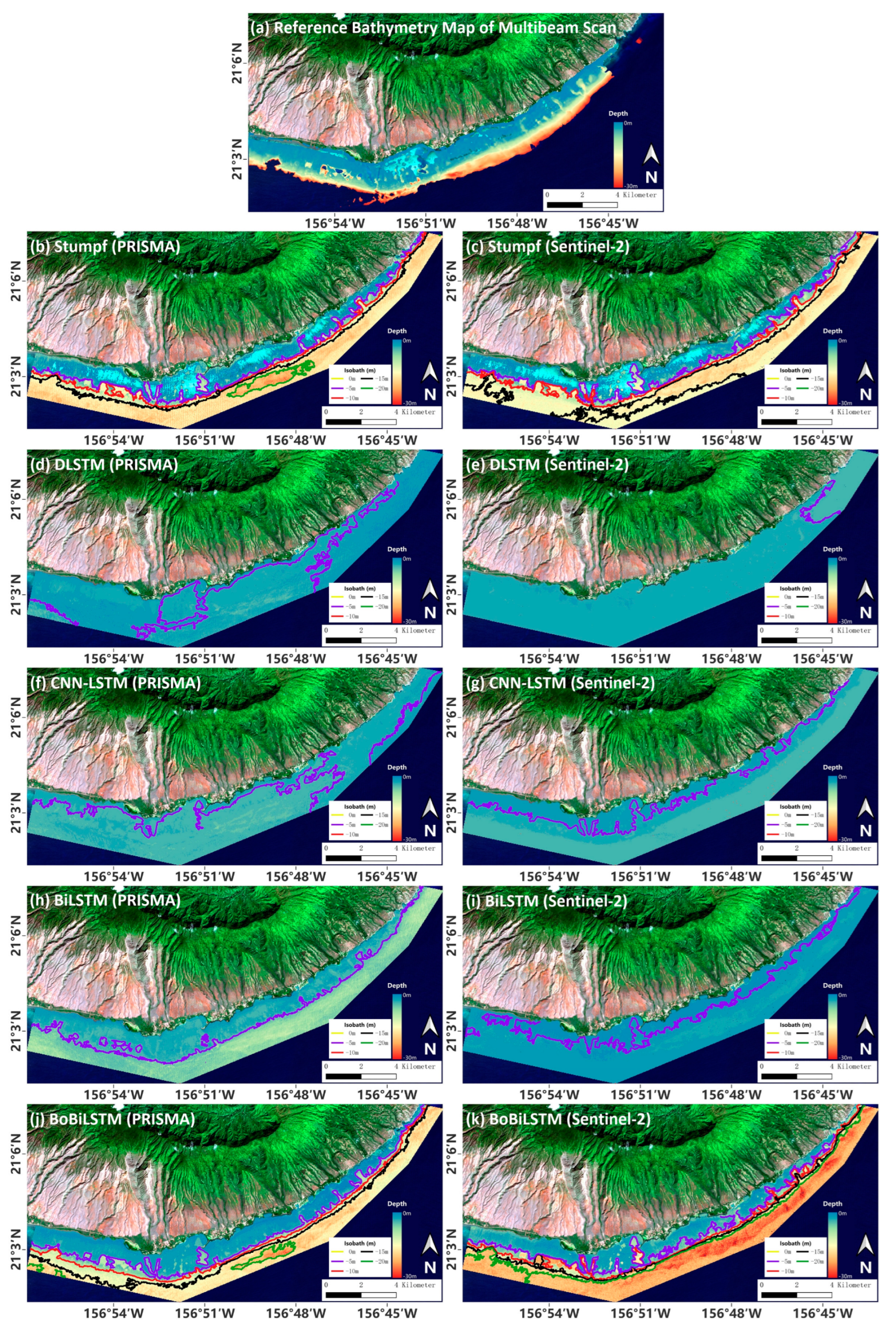
The bathymetry inversion maps generated using PRISMA and Sentinel-2 images are shown in Figure 5. The bathymetric maps of all models retain relatively continuous and intuitive isobaths, and intervals of 5 m are used as division points. Compared to the reference bathymetry map [72], which has a spatial resolution of 2 m, the bathymetry maps inverted using the DLSTM, BiLSTM, and BoBiLSTM models match the reference bathymetry map better than the bathymetry maps inverted using the Stumpf model. They are suitable for hyperspectral and multispectral images. The bathymetry inversion effect of the CNN-LSTM model on the Sentinel-2 image (Figure 5g) is good, but it is very poor on the PRISMA image (Figure 5f). It shows that the CNN-LSTM model is more suitable for bathymetry inversion of multispectral images.
However, there are of course some obvious differences in some patch areas. The optimal band and band ratio selected from the PRISMA image contain more spectral information, so all points on the inverted bathymetry map tend to be smooth and the transition of bathymetry fluctuations is relatively smooth. For the PRISMA image, the DLSTM model (Figure 5d), BiLSTM model (Figure 5h), and BoBiLSTM model (Figure 5j) are relatively similar in the shallow water area within 5 m. The DLSTM model significantly underestimated water depth from 10 m to 15 m, the BiLSTM model significantly underestimated water depth greater than 20 m, and the BoBiLSTM model significantly overestimated water depth greater than 25 m.
The Sentinel-2 image has a wider frequency band and adjacent pixels in the bathymetry inversion image contain similar water depth information, with the edges thus appearing jagged in the water depth fluctuation. For Sentinel-2 images, the DLSTM model (Figure 5e), CNN-LSTM model (Figure 5g), and BoBiLSTM model (Figure 5k) are similar in shallow water areas within 5 m. However, the BiLSTM model overestimated in shallow water areas within 5 m. The CNN-LSTM model and the BiLSTM model had similar accuracy in bathymetry inversion when water depth exceeded 20 m. The BoBiLSTM model underestimated when water depth exceeded 20 m. Compared to the reference bathymetry map, the bathymetry performance of the BoBiLSTM model based on the PRISMA image is higher than that of the BoBiLSTM model based on the Sentinel-2 image.
3.2. Bathymetry Inversion Using Multibeam Scan Data
Compared to the ICESat-2 sensor, the multibeam sensor can detect the ocean floor to a depth of several thousand meters; therefore, it is a good idea to use multibeam data to test whether the proposed BoBiLSTM model’s performance is consistent with ICESat-2 data and test the maximum depth that can be inverted. In this experiment, the data volume of the multibeam sensor is relatively small (only 751 points used), so the inversion accuracy of the deep learning model on the test set in this study area may be high, but the water depth inversion of the entire image has overfitting. Among the 751 points, 601 points are used for training and 150 points are used for testing.
The results of multibeam bathymetry inversion are shown in Table 6. Due to the small amount of multibeam scan data, the BoBiLSTM model was used to explore the relationships between bands and water depth. The highest correlation between PRISMA image bands and water depth changed to band 43 and band 44, and the sum of the contribution values was close to 0.6. Compared with ICESat-2, the proportion of other bands is slightly increased and can also reach 30% of the water depth contribution: 7 and 27 in the near-red range; 40, 41, 42, 45, 46, 47, 48, and 49 in the green range; 54 and 56 in the blue range; and 62, 63, 64, and 65 in the coastal blue range. The most commonly used band combination selected by the Stumpf model is blue–green bands 49 and 56. In the Sentinel-2 image, the bands selected by the BoBiLSTM model that account for the largest proportion of the multibeam scan data are green bands, with an eigenvalue of 0.833.
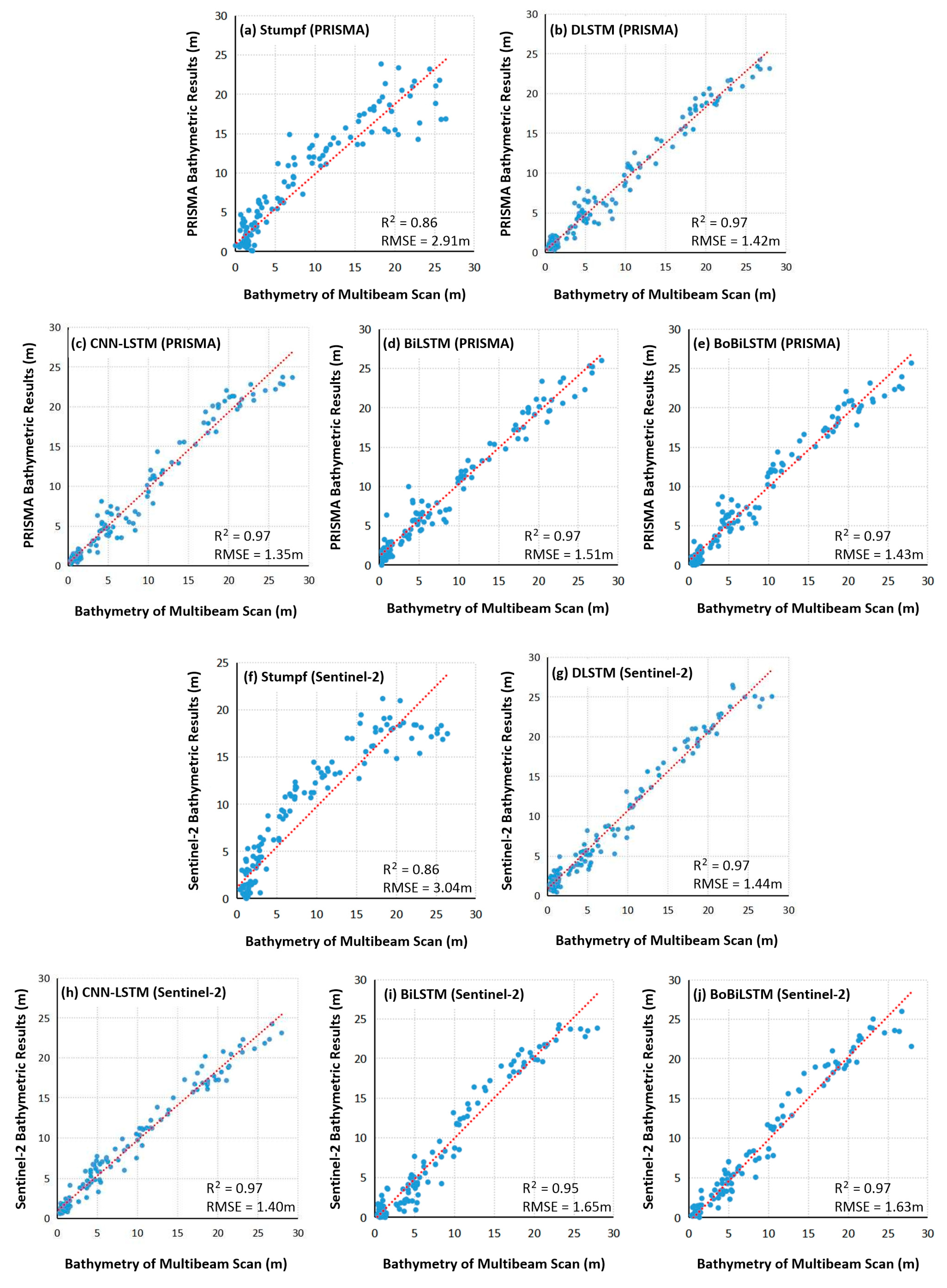
Compared to the traditional Stumpf model, the deep learning models have high correlation, with R2 values of 0.97 and RMSE values of about 1.5 m. Since there are only 150 water depth points in the test set, the RMSE difference of all deep learning models is not very large. Therefore, it is more accurate to analyze water depth inversion accuracy in combination with Figure 6 in this experiment. The BiLSTM model (Figure 6d) and BoBiLSTM model (Figure 6e), using the PRISMA image, can measure water depth values greater than 25 m, and the BoBiLSTM model achieved the best results (R2, 0.97; RMSE, 1.43 m). The test set results of the DLSTM model and BoBiLSTM model are similar within a water depth of 20 m. When the Sentinel-2 image was used, the DLSTM model (Figure 6g) and BoBiLSTM model (Figure 6j) could measure water depths greater than 25 m, while other deep learning models (Figure 6h,i) could only measure water depths within 25 m. It is also worth mentioning that compared to the Sentinel-2 image’s results, the accuracy of the PRISMA image’s results was significantly improved when water depth was more than 20 m (see the comparisons in Figure 8).
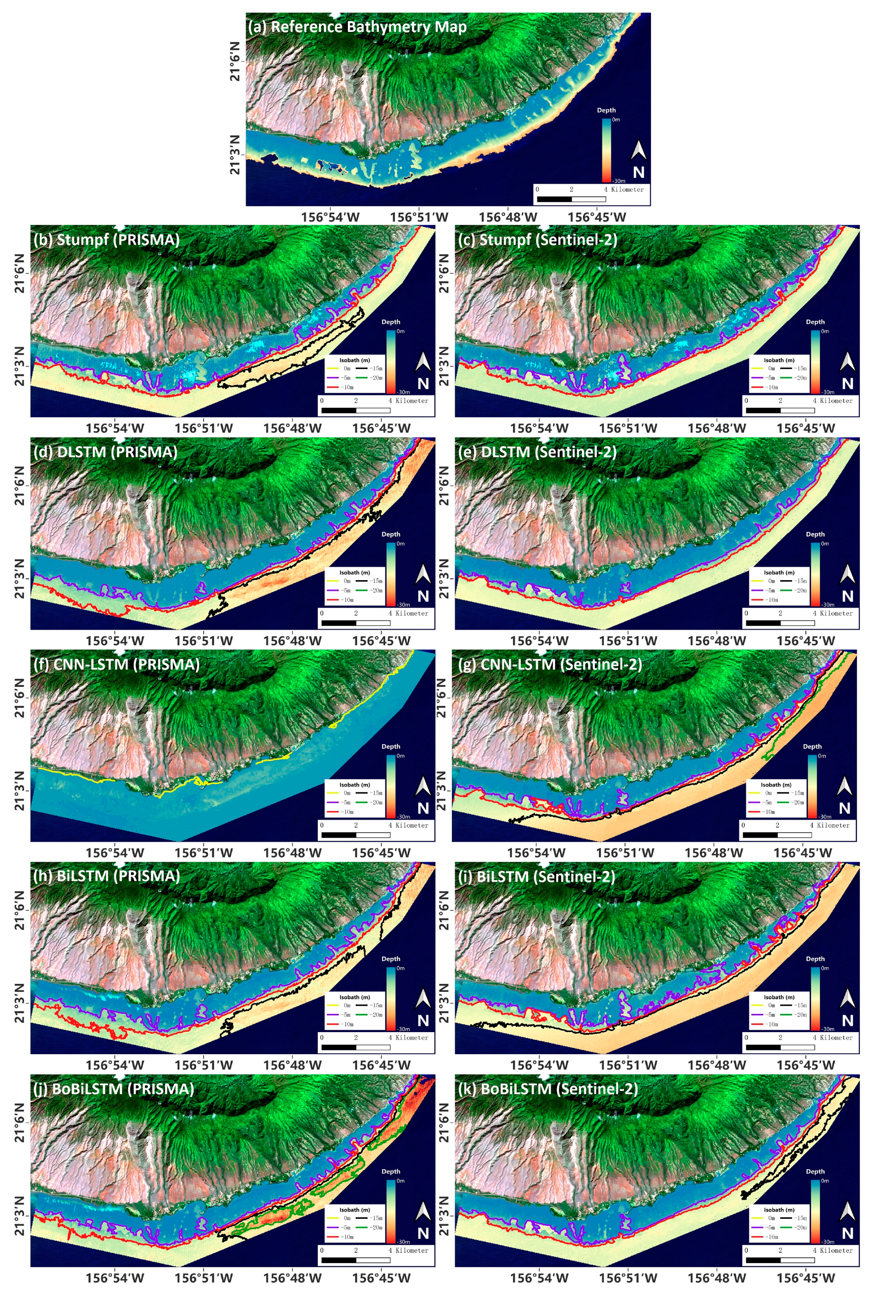
The bathymetry inversion maps generated using PRISMA and Sentinel-2 images are shown in Figure 6. The bathymetry maps of all models retain relatively continuous and intuitive isobaths, and intervals of 5 m are used as division points. When the multibeam scanning data have fewer samples and more band characteristics, the bathymetry inversion of the Stumpf model predicts more water depth values greater than 0 m. The DLSTM model (Figure 7d,e), CNN-LSTM model (Figure 7f,g), and BiLSTM model (Figure 7h,i) have poor water depth retrieval results with the PRISMA image and Sentinel-2 image and cannot clearly distinguish the gradient change in the underwater topography of the area within 20 m. This shows that these models are overfitting in the process of predicting water depth. However, the effect of the bathymetry inversion map of the BiLSTM model is higher than that of the previous two models, and the texture details of water depth can also be identified, especially with the PRISMA image (Figure 7h). This result also confirms the original conjecture of this study, which is that the BiLSTM model can store bidirectional encoding information at the same time. Based on this model, it is further proposed that the BoBiLSTM model is more suitable as a deep learning model for bathymetry inversion. The bathymetry inversion map of the PRISMA image made using the BoBiLSTM model (Figure 7j) is similar to the multibeam bathymetric map (Figure 7a) and can describe changes in bathymetric texture. Whether in shallow water or deep water, the bathymetric inversion effect of this model is very good. The BoBiLSTM model (Figure 7k) based on the Sentinel-2 image can identify shallow and deep water areas, but bathymetric measurements beyond 15 m are overestimated.
4. Discussions
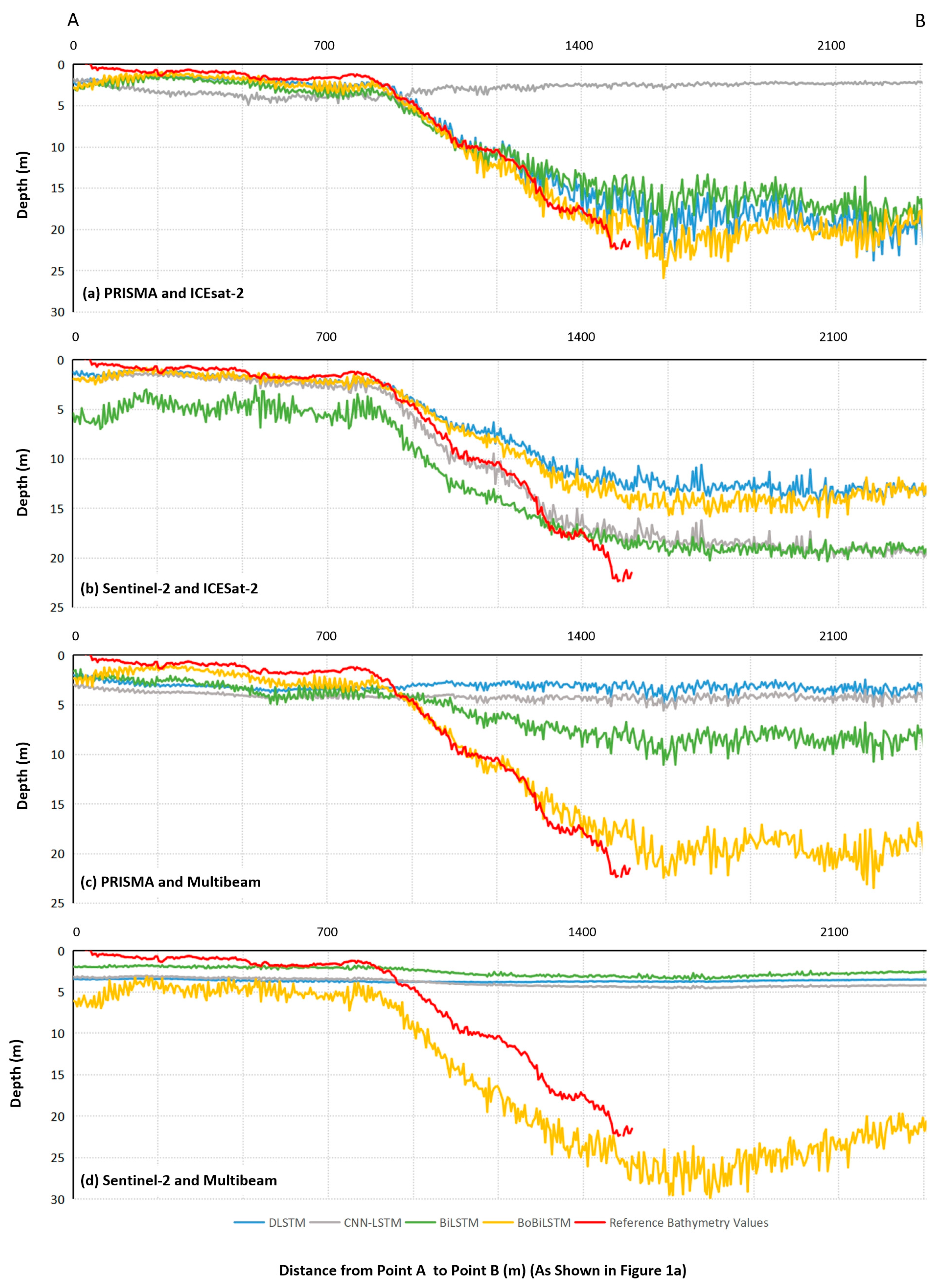
This paper proposes a BoBiLSTM model that combines in situ water depth with band reflectance from satellite imagery for important feature selection. The model can bidirectionally learn water depth information both in shallow water areas and the relatively deeper water areas through the bidirectional configuration of the network, thus obtaining more characteristics for sensitive water surface reflectance. By adding the band optimization layer, the BoBiLSTM model can capture the important sequence information of each batch of training sets and provide more information about the water column and bottom conditions in a more efficient and lightweight way. In order to evaluate the robustness of different deep learning models, we plotted the depth profiles of a line segment (the AB line in Figure 1a) to compare the results inverted by the four deep learning models against the reference bathymetry values, as shown in Figure 8. Through this study, it can be seen that the proposed BoBiLSTM model could accurately detect and select the most important bands for water depth inversion when either ICESat-2 or multibeam data were used. Previous studies have applied water depths in different depth ranges according to the water surface reflectance in different bands [24,83]. As the water depth decreases, the sensitive band of water body reflection changes from the green band to the near-red band [83], and the bathymetric contribution in extremely shallow areas cannot be ignored [84]. In this study, these factors are largely considered by the BoBiLSTM model, which can extract the water depth information contained in important bands and band ratios without dividing the depth into segments, with the accuracy of bathymetry inversion in the entire region thus significantly improved.
In this study, ICESat-2 provided less training points for areas where water depth is beyond 20 m, which is mainly due to the fact that as the water depth increases, more laser energy is absorbed by the water column, resulting in insufficient bottom reflection energy [65]; thus, the errors in predicting deep water areas will also increase. On the other hand, when multibeam data were used as training data, bathymetric maps with relatively high accuracy could be generated from the PRISMA image (Figure 7j). This is mainly due to evenly distributed multibeam sounding points both in planimetric and vertical directions because, unlike ICESat-2, multibeam sounding systems are capable of measuring points at any depth. When water depth exceeded 15 m, bathymetric accuracy with the Sentinel-2 image decreased significantly and the attenuation effect of depth changes on the near-red band was more obvious [26,28]. Table 7 shows a comparison of errors between the bathymetry maps retrieved from the PRISMA image and the Sentinel-2 image using different deep learning models and the reference bathymetry map. The maximum depth of the reference bathymetry map for this study area is 33.38 m, while the PRISMA image predicts a depth of more than 25 m (RMSE of 2.35 m) and the Sentinel-2 image predicts a depth of about 20 m (RMSE of 2.47 m). For the PRISMA image, the bathymetry inversion map generated using multibeam data is comparable to that of the map made using ICESat-2 data, thus verifying that the proposed BoBiLSTM model has stronger robustness and achieves higher bathymetry accuracy. In summary, either using ICESat-2 data or multibeam data as training data, the hyperspectral images (PRISMA) provide higher quality bathymetric maps than multispectral images (Sentinel-2) do in SDB.
This study verified whether the bathymetry map generated by the BoBiLSTM model combined with hyperspectral image (PRISMA) meets the S-57 standard [85] (Table 8). For the S-57 standard, the bathymetry maps retrieved by the BoBiLSTM model exceed the A2 and B level in both shallow and deep areas of water and therefore can be used as navigation information according to the International Hydrographic Organization (IHO). However, more comprehensive tests are required to support this claim.
5. Conclusions
In this study, we proposed the BoBiLSTM model for bathymetry inversion from satellite imagery. This model can bidirectionally encode water depth information both in shallow and relatively deeper water areas and acquire more characteristics of the sensitive bands of off-water reflectance. Both traditional empirical models and semi-analytical models use single-band or dual-band photogrammetry for bathymetry inversion, which cannot accurately represent the physical mechanism of bathymetry for hyperspectral images and multispectral images. The BoBiLSTM model provides the reflectivity information of more important bands in a more lightweight and robust way. It eliminates band information that contributes less to bathymetry inversion in hyperspectral or multispectral images and overcomes the disadvantage that deep learning models usually face in terms of requiring a large amount of training data. A series of experiments were conducted in the southeast of Molokai Island. The experimental results show that when the BoBiLSTM model is applied to a PRISMA image, it achieves RMSE values of 0.82 m (ICESat-2 as training data) and 1.43 m (multibeam as training data), and when the BoBiLSTM model is applied to a Sentinel-2 image, it achieves slightly lower RMSE values of 1.08 m (ICESat-2 as training data) and 1.63 m (multibeam as training data). Because the PRISMA images are rich in spectral information compared to multispectral images like Sentinel-2 images, more depth information can be retrieved when PRISMA images are used (beyond 25 m deep) compared to when Sentinel-2 images are used (around 20 m deep). Therefore, it can be concluded that the BoBiLSTM model is more robust than the Stumpf, DLSTM, CNN-LSTM, and BiLSTM models. The BoBiLSTM model also has exceptional performance in relatively deeper ranges, which is quite important if SDB models are to be used operationally. Through comparative analysis with the IHO standard, the bathymetry map generated using the BoBiLSTM model and the hyperspectral images (PRISMA) meets the requirements of S-57 for both shallow and relatively deeper water areas. Therefore, the proposed BoBiLSTM model has great potential in operational use of bathymetry. Future, studies will explore the use of the BoBiLSTM model in different environments and apply it to different sensors, like EnMAP, while making the model more user-friendly for people to be able explore other applications, such as multi-temporal bathymetry inversion and the classification of seabed topography.
Author Contributions
Conceptualization, investigation, methodology, experiment analysis, writing—original draft preparation, X.X.; conceptualization, supervision, writing—review and editing, M.C.; data curation, validation, visualization, H.Y. and Y.W. All authors have read and agreed to the published version of the manuscript.
Funding
This study was funded by Shanghai Science and Technology Innovation Action Planning, No.20dz1203800.
Data Availability Statement
The ICESat-2 datasets are available from https://nsidc.org/data/atl03/versions/5 (accessed on 15 September 2022). The multibeam scan data were accessed from http://www.soest.hawaii.edu/HMRG/multibeam/index.php (accessed on 15 September 2022). The bathymetry data maps were created by the Global Airborne Observatory, Center for Global Discovery and Conservation Science, Arizona State University, and are available from references [72] and [73]. The PRISMA image is available from https://prisma.asi.it/ (accessed on 15 September 2022). The Sentinel-2 image is available from https://scihub.copernicus.eu/dhus/#/home (accessed on 15 September 2022).
Acknowledgments
The authors gratefully thank the following organizations for providing the experimental datasets: NASA, ESA (European Space Agency), and ASI (Italian Space Agency) for providing satellite data from ICESat-2, Sentinel-2, and PRISMA, respectively.; the Global Airborne Observatory, Center for Global Discovery and Conservation Science, Arizona State University, for providing reference bathymetry maps; and the Hawaii Undersea Research Laboratory, NOAA’s Pacific Islands Benthic Habitat Mapping Center, and the Schmidt Ocean Institute for providing multibeam bathymetry data.
Conflicts of Interest
The authors declare no conflict of interest.
References
- Lyons, M.; Phinn, S.; Roelfsema, C. Integrating Quickbird Multi-Spectral Satellite and Field Data: Mapping Bathymetry, Seagrass Cover, Seagrass Species and Change in Moreton Bay, Australia in 2004 and 2007. Remote Sens. 2011, 3, 42–64. [Google Scholar] [CrossRef] [Green Version]
- Kutser, T.; Hedley, J.; Giardino, C.; Roelfsema, C.; Brando, V.E. Remote Sensing of Shallow Waters—A 50 Year Retrospective and Future Directions. Remote Sens. Environ. 2020, 240, 111619. [Google Scholar] [CrossRef]
- Storlazzi, C.D.; Logan, J.B.; Field, M.E. Quantitative Morphology of A Fringing Reef Tract from High-resolution Laser Bathymetry Southern Molokai, Hawaii. Geol. Soc. Am. Bull. 2003, 115, 1344. [Google Scholar] [CrossRef]
- Wölfl, A.-C.; Snaith, H.; Amirebrahimi, S.; Devey, C.W.; Dorschel, B.; Ferrini, V.; Huvenne, V.A.I.; Jakobsson, M.; Jencks, J.; Johnston, G.; et al. Seafloor Mapping—The Challenge of a Truly Global Ocean Bathymetry. Front. Mar. Sci. 2019, 6, 283. [Google Scholar] [CrossRef] [Green Version]
- Jörges, C.; Berkenbrink, C.; Stumpe, B. Prediction and Reconstruction of Ocean Wave Heights Based on Bathymetric Data Using LSTM Neural Networks. Ocean Eng. 2021, 232, 109046. [Google Scholar] [CrossRef]
- Shang, X.; Zhao, J.; Zhang, H. Obtaining High-Resolution Seabed Topography and Surface Details by Co-Registration of Side-Scan Sonar and Multibeam Echo Sounder Images. Remote Sens. 2019, 11, 1496. [Google Scholar] [CrossRef] [Green Version]
- National Oceanic and Atmospheric Administration (NOAA): Field Procedures Manual. Available online: https://nauticalcharts.noaa.gov/publications/docs/standards-and-requirements/fpm/2014-fpm-final.pdf (accessed on 15 September 2022).
- Westfeld, P.; Maas, H.-G.; Richter, K.; Weiß, R. Analysis and Correction of Ocean Wave Pattern Induced Systematic Coordinate Errors in Airborne LiDAR Bathymetry. ISPRS J. Photogramm. Remote Sens. 2017, 128, 314–325. [Google Scholar] [CrossRef]
- Pan, Z.; Glennie, C.; Hartzell, P.; Fernandez-Diaz, J.; Legleiter, C.; Overstreet, B. Performance Assessment of High Resolution Airborne Full Waveform LiDAR for Shallow River Bathymetry. Remote Sens. 2015, 7, 5133–5159. [Google Scholar] [CrossRef] [Green Version]
- Zhao, J.; Zhao, X.; Zhang, H.; Zhou, F. Improved Model for Depth Bias Correction in Airborne LiDAR Bathymetry Systems. Remote Sens. 2017, 9, 710. [Google Scholar] [CrossRef] [Green Version]
- Zhang, X.; Chen, Y.; Le, Y.; Zhang, D.; Yan, Q.; Dong, Y.; Han, W.; Wang, L. Nearshore Bathymetry Based on ICESat-2 and Multispectral Images: Comparison Between Sentinel-2, Landsat-8, and Testing Gaofen-2. IEEE J. Sel. Top. Appl. Earth Obs. Remote Sens. 2022, 15, 2449–2462. [Google Scholar] [CrossRef]
- Muzirafuti, A.; Crupi, A.; Lanza, S.; Barreca, G.; Randazzo, G. Shallow water bathymetry by satellite image: A case study on the coast of San Vito Lo Capo Peninsula, Northwestern Sicily, Italy. In Proceedings of the IMEKO TC-19 International Workshop on Metrology for the Sea, Genoa, Italy, 3–5 October 2019. [Google Scholar]
- Almar, R.; Bergsma, E.W.J.; Thoumyre, G.; Baba, M.W.; Cesbron, G.; Daly, C.; Garlan, T.; Lifermann, A. Global Satellite-Based Coastal Bathymetry from Waves. Remote Sens. 2021, 13, 4628. [Google Scholar] [CrossRef]
- Danilo, C.; Melgani, F. High-Coverage Satellite-Based Coastal Bathymetrythrough a Fusion of Physical and Learning Methods. Remote Sens. 2019, 11, 376. [Google Scholar] [CrossRef] [Green Version]
- Cao, B.; Fang, Y.; Jiang, Z.; Gao, L.; Hu, H. Shallow Water Bathymetry from WorldView-2 Stereo Imagery Using Two-media Photogrammetry. Eur. J. Remote Sens. 2019, 52, 506–521. [Google Scholar] [CrossRef] [Green Version]
- Mishra, M.K.; Ganguly, D.; Chauhan, P.; Ajai. Estimation of Coastal Bathymetry Using RISAT-1 C-Band Microwave SAR Data. IEEE Geosci. Remote Sens. Lett. 2014, 11, 671–675. [Google Scholar] [CrossRef]
- Specht, M.; Stateczny, A.; Specht, C.; Widźgowski, S.; Lewicka, O.; Wiśniewska, M. Concept of an Innovative Autonomous Unmanned System for Bathymetric Monitoring of Shallow Waterbodies (INNOBAT System). Energies 2021, 14, 5370. [Google Scholar] [CrossRef]
- Specht, M.; Wisniewska, M.; Stateczny, A.; Specht, C.; Szostak, B.; Lewicka, O.; Stateczny, M.; Widzgowski, S.; Halicki, A. Analysis of Methods for Determining Shallow Waterbody Depths Based on Images Taken by Unmanned Aerial Vehicles. Sensors 2022, 22, 1844. [Google Scholar] [CrossRef] [PubMed]
- Lewicka, O.; Specht, M.; Stateczny, A.; Specht, C.; Dardanelli, G.; Brčić, D.; Szostak, B.; Halicki, A.; Stateczny, M.; Widźgowski, S. Integration Data Model of the Bathymetric Monitoring System for Shallow Waterbodies Using UAV and USV Platforms. Remote Sens. 2022, 14, 4075. [Google Scholar] [CrossRef]
- Najar, M.A.; Bennioui, Y.E.; Thoumyre, G.; Almar, R.; Bergsma, E.W.J.; Benshila, R.; Delvit, J.-M.; Wilson, D.G. A Combined Color and Wave-Based Approach to Satellite Derived Bathymetry Using Deep Learning. In Proceedings of the The International Archives of the Photogrammetry, Remote Sensing and Spatial Information Sciences, Nice, France, 6–11 June 2022; Volume XLIII-B3-2022, pp. 9–16. [Google Scholar] [CrossRef]
- Jawak, S.D.; Vadlamani, S.S.; Luis, A.J. A Synoptic Review on Deriving Bathymetry Information Using Remote Sensing Technologies: Models, Methods and Comparisons. Adv. Remote Sens. 2015, 4, 147–162. [Google Scholar] [CrossRef] [Green Version]
- Casal, G.; Monteys, X.; Hedley, J.; Harris, P.; Cahalane, C.; McCarthy, T. Assessment of Empirical Algorithms for Bathymetry Extraction Using Sentinel-2 Data. Int. J. Remote Sens. 2018, 40, 2855–2879. [Google Scholar] [CrossRef]
- Yunus, A.P.; Dou, J.; Song, X.; Avtar, R. Improved Bathymetric Mapping of Coastal and Lake Environments Using Sentinel-2 and Landsat-8 Images. Sensors 2019, 19, 2788. [Google Scholar] [CrossRef] [Green Version]
- Amrari, S.; Bourassin, E.; Andréfouët, S.; Soulard, B.; Lemonnier, H.; Le Gendre, R. Shallow Water Bathymetry Retrieval Using a Band-Optimization Iterative Approach: Application to New Caledonia Coral Reef Lagoons Using Sentinel-2 Data. Remote Sens. 2021, 13, 4108. [Google Scholar] [CrossRef]
- Lyzenga, D.R. Shallow-water Bathymetry Using Combined Lidar and Passive Multispectral Scanner Data. Int. J. Remote Sens. 2010, 6, 115–125. [Google Scholar] [CrossRef]
- Stumpf, R.; PHolderied, K.; Sinclair, M. Determination of Water Depth with High-resolution Satellite Imagery over Variable Bottom Types. Limnol. Oceanogr. 2003, 48 Pt 2, 547–556. [Google Scholar] [CrossRef]
- Fotheringham, A.S.; Charlton, M.E.; Brunsdon, C. Geographically Weighted Regression: A Natural Evolution of the Expansion Method for Spatial Data Analysis. Environ. Plan. A 1998, 30, 1905–1927. [Google Scholar] [CrossRef]
- Casal, G.; Harris, P.; Monteys, X.; Hedley, J.; Cahalane, C.; McCarthy, T. Understanding Satellite-derived Bathymetry Using Sentinel 2 Imagery and Spatial Prediction Models. GIScience Remote Sens. 2019, 57, 271–286. [Google Scholar] [CrossRef]
- Ceyhun, Ö.; Yalçın, A. Remote Sensing of Water Depths in Shallow Waters via Artificial Neural Networks. Estuar. Coast. Shelf Sci. 2010, 89, 89–96. [Google Scholar] [CrossRef]
- Nagamani, P.V.; Chauhan, P.; Sanwlani, N.; Ali, M.M. Artificial Neural Network (ANN) Based Inversion of Benthic Substrate Bottom Type and Bathymetry in Optically Shallow Waters-Initial Model Results. J. Indian Soc. Remote Sens. 2012, 40, 137–143. [Google Scholar] [CrossRef]
- Liu, S.; Wang, L.; Liu, H.; Su, H.; Li, X.; Zheng, W. Deriving Bathymetry from Optical Images With a Localized Neural Network Algorithm. IEEE Trans. Geosci. Remote Sens. 2018, 56, 5334–5342. [Google Scholar] [CrossRef]
- Niroumand-Jadidi, M.; Legleiter, C.J.; Bovolo, F. River Bathymetry Retrieval From Landsat-9 Images Based on Neural Networks and Comparison to SuperDove and Sentinel-2. IEEE J. Sel. Top. Appl. Earth Obs. Remote Sens. 2022, 15, 5250–5260. [Google Scholar] [CrossRef]
- Zhu, J.; Qin, J.; Yin, F.; Ren, Z.; Qi, J.; Zhang, J.; Wang, R. An APMLP Deep Learning Model for Bathymetry Retrieval Using Adjacent Pixels. IEEE J. Sel. Top. Appl. Earth Obs. Remote Sens. 2022, 15, 235–246. [Google Scholar] [CrossRef]
- Najar, M.A.; Benshila, R.; Bennioui, Y.E.; Thoumyre, G.; Almar, R.; Bergsma, E.W.J.; Delvit, J.-M.; Wilson, D.G. Coastal Bathymetry Estimation from Sentinel-2 Satellite Imagery: Comparing Deep Learning and Physics-Based Approaches. Remote Sens. 2022, 14, 1196. [Google Scholar] [CrossRef]
- Alevizos, E.; Nicodemou, V.C.; Makris, A.; Oikonomidis, I.; Roussos, A.; Alexakis, D.D. Integration of Photogrammetric and Spectral Techniques for Advanced Drone-Based Bathymetry Retrieval Using a Deep Learning Approach. Remote Sens. 2022, 14, 4160. [Google Scholar] [CrossRef]
- Ai, B.; Wen, Z.; Wang, Z.; Wang, R.; Su, D.; Li, C.; Yang, F. Convolutional Neural Network to Retrieve Water Depth in Marine Shallow Water Area from Remote Sensing Images. IEEE J. Sel. Top. Appl. Earth Obs. Remote Sens. 2020, 13, 2888–2898. [Google Scholar] [CrossRef]
- Wilson, B.; Kurian, N.C.; Singh, A.; Sethi, A. Satellite-Derived Bathymetry Using Deep Convolutional Neural Network. In Proceedings of the IGARSS 2020–2020 IEEE International Geoscience and Remote Sensing Symposium, Waikoloa, HI, USA, 26 September–2 October 2020; pp. 2280–2283. [Google Scholar]
- Markus, T.; Neumann, T.; Martino, A.; Abdalati, W.; Brunt, K.; Csatho, B.; Farrell, S.; Fricker, H.; Gardner, A.; Harding, D.; et al. The Ice, Cloud, and Land Elevation Satellite-2 (ICESat-2): Science Requirements, Concept, and Implementation. Remote Sens. Environ. 2017, 190, 260–273. [Google Scholar] [CrossRef]
- Malambo, L.; Popescu, S. PhotonLabeler: An Inter-Disciplinary Platform for Visual Interpretation and Labeling of ICESat-2 Geolocated Photon Data. Remote Sens. 2020, 12, 3168. [Google Scholar] [CrossRef]
- Guo, X.; Jin, X.; Jin, S. Shallow Water Bathymetry Mapping from ICESat-2 and Sentinel-2 Based on BP Neural Network Model. Water 2022, 14, 3862. [Google Scholar] [CrossRef]
- Zhong, J.; Sun, J.; Lai, Z.; Song, Y. Nearshore Bathymetry from ICESat-2 LiDAR and Sentinel-2 Imagery Datasets Using Deep Learning Approach. Remote Sens. 2022, 14, 4229. [Google Scholar] [CrossRef]
- Yang, H.; Chen, M.; Wu, G.; Wang, J.; Wang, Y.; Hong, Z. Double Deep Q-Network for Hyperspectral Image Band Selection in Land Cover Classification Applications. Remote Sens. 2023, 15, 682. [Google Scholar] [CrossRef]
- Wang, J.; Chen, M.; Zhu, W.; Hu, L.; Wang, Y. A Combined Approach for Retrieving Bathymetry from Aerial Stereo RGB Imagery. Remote Sens. 2022, 14, 760. [Google Scholar] [CrossRef]
- Alevizos, E.; Oikonomou, D.; Argyriou, A.V.; Alexakis, D.D. Fusion of Drone-Based RGB and Multi-Spectral Imagery for Shallow Water Bathymetry Inversion. Remote Sens. 2022, 14, 1127. [Google Scholar] [CrossRef]
- Rossi, L.; Mammi, I.; Pelliccia, F. UAV-Derived Multispectral Bathymetry. Remote Sens. 2020, 12, 3897. [Google Scholar] [CrossRef]
- Evagorou, E.; Argyriou, A.; Papadopoulos, N.; Mettas, C.; Alexandrakis, G.; Hadjimitsis, D. Evaluation of Satellite-Derived Bathymetry from High and Medium-Resolution Sensors Using Empirical Methods. Remote Sens. 2022, 14, 772. [Google Scholar] [CrossRef]
- Zhang, D.; Guo, Q.; Cao, L.; Zhou, G.; Zhang, G.; Zhan, J. A Multiband Model With Successive Projections Algorithm for Bathymetry Estimation Based on Remotely Sensed Hyperspectral Data in Qinghai Lake. IEEE J. Sel. Top. Appl. Earth Obs. Remote Sens. 2021, 14, 6871–6881. [Google Scholar] [CrossRef]
- Alevizos, E. A Combined Machine Learning and Residual Analysis Approach for Improved Retrieval of Shallow Bathymetry from Hyperspectral Imagery and Sparse Ground Truth Data. Remote Sens. 2020, 12, 3489. [Google Scholar] [CrossRef]
- Niroumand-Jadidi, M.; Bovolo, F.; Bruzzone, L. SMART-SDB: Sample-specific Multiple Band Ratio Technique for Satellite-Derived Bathymetry. Remote Sens. Environ. 2020, 251, 112091. [Google Scholar] [CrossRef]
- Cheng, L.; Ma, L.; Cai, W.; Tong, L.; Li, M.; Du, P. Integration of Hyperspectral Imagery and Sparse Sonar Data for Shallow Water Bathymetry Mapping. IEEE Trans. Geosci. Remote Sens. 2015, 53, 3235–3249. [Google Scholar] [CrossRef]
- Cui, J.; Kong, W.; Zhang, X.; Chen, D.; Zeng, Q. DLSTM-Based Successive Cancellation Flipping Decoder for Short Polar Codes. Entropy 2021, 23, 863. [Google Scholar] [CrossRef] [PubMed]
- Liu, S.; Zhang, C.; Ma, J. CNN-LSTM Neural Network Model for Quantitative Strategy Analysis in Stock Markets. In Neural Information Processing; Lecture Notes in Computer Science; Springer: Cham, Switzerland, 2017; pp. 198–206. [Google Scholar]
- Ghasemlounia, R.; Gharehbaghi, A.; Ahmadi, F.; Saadatnejadgharahassanlou, H. Developing a Novel Framework for Forecasting Groundwater Level Fluctuations Using Bi-directional Long Short-Term Memory (BiLSTM) Deep Neural Network. Comput. Electron. Agric. 2021, 191, 106568. [Google Scholar] [CrossRef]
- Friedman, J.H. Greedy Function Approximation: A Gradient Boosting Machine. Ann. Stat. 2001, 29, 1189–1232. [Google Scholar] [CrossRef]
- Ghimire, S.; Yaseen, Z.M.; Farooque, A.A.; Deo, R.C.; Zhang, J.; Tao, X. Streamflow Prediction Using An Integrated Methodology Based on Convolutional Neural Network and Long Short-term Memory Networks. Sci. Rep. 2021, 11, 17497. [Google Scholar] [CrossRef] [PubMed]
- Peng, Y.; Liu, X.; Wang, W.; Zhao, X.; Wei, M. Image Caption Model of Double LSTM with Scene Factors. Image Vis. Comput. 2019, 86, 38–44. [Google Scholar] [CrossRef]
- Zhang, J.; Pei, Z.; Luo, Z. Reasoning for Local Graph Over Knowledge Graph With a Multi-Policy Agent. IEEE Access 2021, 9, 78452–78462. [Google Scholar] [CrossRef]
- PRISMA Data. Available online: https://prisma.asi.it/ (accessed on 15 September 2022).
- PRISMA User Manual. Available online: http://prisma.asi.it/missionselect/docs/PRISMA%20User%20Manual_Is1_3.pdf (accessed on 15 September 2022).
- ESA Copernicus Data Center. Available online: https://scihub.copernicus.eu/dhus/#/home (accessed on 15 September 2022).
- SNAP Download. Available online: http://step.esa.int/main/download/snap-download/ (accessed on 15 September 2022).
- Sentinel-2 User Handbook. Available online: https://sentinel.esa.int/documents/247904/685211/Sentinel-2_User_Handbook (accessed on 15 September 2022).
- Neumann, T.; Brenner, A.; Hancock, D.; Robbins, J.; Saba, J.; Harbeck, K. Ice, Cloud, and Land Elevation Satellite-2 (ICESat-2) Project: Algorithm Theoretical Basis Document (ATBD) for Global Geolocated Photons (ATL03). Available online: https://icesat-2.gsfc.nasa.gov/sites/default/files/files/ATL03_05June2018.pdf (accessed on 15 September 2022).
- Parrish, C.E.; Magruder, L.A.; Neuenschwander, A.L.; Forfinski-Sarkozi, N.; Alonzo, M.; Jasinski, M. Validation of ICESat-2 ATLAS Bathymetry and Analysis of ATLAS’s Bathymetric Mapping Performance. Remote Sens. 2019, 11, 1634. [Google Scholar] [CrossRef] [Green Version]
- Le, Y.; Hu, M.; Chen, Y.; Yan, Q.; Zhang, D.; Li, S.; Zhang, X.; Wang, L. Investigating the Shallow-Water Bathymetric Capability of Zhuhai-1 Spaceborne Hyperspectral Images Based on ICESat-2 Data and Empirical Approaches: A Case Study in the South China Sea. Remote Sens. 2022, 14, 3406. [Google Scholar] [CrossRef]
- Chen, Y.; Zhu, Z.; Le, Y.; Qiu, Z.; Chen, G.; Wang, L. Refraction Correction and Coordinate Displacement Compensation in Nearshore Bathymetry Using ICESat-2 Lidar Data and Remote-sensing Images. Opt. Express 2021, 29, 2411–2430. [Google Scholar] [CrossRef] [PubMed]
- Ester, M.; Kriegel, H.-P.; Sander, J.; Xu, X. A Density-based Algorithm for Discovering Clusters in Large Spatial Databases with Noise. In Proceedings of the Second International Conference on Knowledge Discovery and Data Mining, Portland, OR, USA, 2–4 August 1996; pp. 226–231. [Google Scholar]
- NOAA Tides and Currents. Available online: https://tidesandcurrents.noaa.gov (accessed on 15 September 2022).
- Richards, B.L.; Smith, J.R.; Smith, S.G.; Ault, J.S.; Kelley, C.D.; Moriwake, V.N. A Five-meter Resolution Multi-Beam Bathymetric and Backskatter Synthesis for the Main Hawaiian Islands. Available online: http://www.soest.hawaii.edu/HMRG/multibeam/index.php (accessed on 15 September 2022).
- Smith, J.R. Multibeam Backscatter and Bathymetry Synthesis for the Main Hawaiian Islands, Final Technical Report; NOAA: Silver Spring, MD, USA, 2016; pp. 1–15. [Google Scholar]
- Chen, Y.; Le, Y.; Zhang, D.; Wang, Y.; Qiu, Z.; Wang, L. A Photon-counting LiDAR Bathymetric Method Based on Adaptive Variable Ellipse Filtering. Remote Sens. Environ. 2021, 256, 112326. [Google Scholar] [CrossRef]
- Asner, G.P.; Vaughn, N.R.; Balzotti, C.; Brodrick, P.G.; Heckler, J. High-Resolution Reef Bathymetry and Coral Habitat Complexity from Airborne Imaging Spectroscopy. Remote Sens. 2020, 12, 310. [Google Scholar] [CrossRef] [Green Version]
- Asner, G.P.; Vaughn, N.R.; Foo, S.A.; Shafron, E.; Heckler, J.; Martin, R.E. Abiotic and Human Drivers of Reef Habitat Complexity Throughout the Main Hawaiian Islands. Front. Mar. Sci. 2021, 8, 631842. [Google Scholar] [CrossRef]
- Hochreiter, S.; Schmidhuber, J. Long Short-Term Memory. Neural Comput. 1997, 9, 1735–1780. [Google Scholar] [CrossRef]
- Schuster, M.; Paliwal, K.K. Bidirectional Recurrent Neural Networks. IEEE Trans. Signal Process. 1997, 45, 2673–2681. [Google Scholar] [CrossRef] [Green Version]
- Yuan, X.; Wang, X.; Han, J.; Liu, J.; Chen, H.; Zhang, K.; Ye, Q. A High Accuracy Integrated Bagging-Fuzzy-GBDT Prediction Algorithm for Heart Disease Diagnosis. In Proceedings of the 2019 IEEE/CIC International Conference on Communications in China (ICCC), Changchun, China, 11–13 August 2019. [Google Scholar]
- Friedman, J.H. Stochastic Gradient Boosting. Comput. Stat. Data Anal. 2002, 38, 367–378. [Google Scholar] [CrossRef]
- Cheng, J.; Li, G.; Chen, X. Research on Travel Time Prediction Model of Freeway Based on Gradient Boosting Decision Tree. IEEE Access 2019, 7, 7466–7480. [Google Scholar] [CrossRef]
- Song, Y.; Niu, R.; Xu, S.; Ye, R.; Peng, L.; Guo, T.; Li, S.; Chen, T. Landslide Susceptibility Mapping Based on Weighted Gradient Boosting Decision Tree in Wanzhou Section of the Three Gorges Reservoir Area (China). ISPRS Int. J. Geo. Inf. 2018, 8, 4. [Google Scholar] [CrossRef] [Green Version]
- Zhang, Z.; Jung, C. GBDT-MO Gradient-Boosted Decision Trees for Multiple Outputs. IEEE Trans. Neural Netw. Learn. Syst. 2020, 32, 3156–3167. [Google Scholar] [CrossRef]
- Srivastava, N.; Hinton, G.; Krizhevsky, A.; Sutskever, I.; Salakhutdinov, R. Dropout: A Simple Way to Prevent Neural Networks from Overfitting. J. Mach. Learn. Res. 2014, 15, 1929–1958. [Google Scholar]
- Kingma, D.P.; Ba, J. Adam: A Method for Stochastic Optimization. In Proceedings of the the 3rd International Conference for Learning Representations (ICLR), San Diego, CA, USA, 7–9 May 2015. [Google Scholar]
- Liu, Y.; Tang, D.; Deng, R.; Cao, B.; Chen, Q.; Zhang, R.; Qin, Y.; Zhang, S. An Adaptive Blended Algorithm Approach for Deriving Bathymetry from Multispectral Imagery. IEEE J. Sel. Top. Appl. Earth Obs. Remote Sens. 2021, 14, 801–817. [Google Scholar] [CrossRef]
- Vahtmäe, E.; Kutser, T. Airborne Mapping of Shallow Water Bathymetry in the Optically Complex Waters of the Baltic Sea. J. Appl. Remote Sens. 2016, 10, 025012. [Google Scholar] [CrossRef]
- Chénier, R.; Faucher, M.-A.; Ahola, R. Satellite-Derived Bathymetry for Improving Canadian Hydrographic Service Charts. ISPRS Int. J. Geo-Inf. 2018, 7, 306. [Google Scholar] [CrossRef] [Green Version]
Figure 1.
(a) Location of shallow water southeast of Molokai, where the depth profile of the AB line will be showcased in the Discussions section later; (b) ICESat-2 strips used as training data (solid lines with different colors); (c) multibeam training data locations.
Figure 1.
(a) Location of shallow water southeast of Molokai, where the depth profile of the AB line will be showcased in the Discussions section later; (b) ICESat-2 strips used as training data (solid lines with different colors); (c) multibeam training data locations.

Figure 2.
Internal logic of the LSTM unit.

Figure 3.
(a) Bathymetry inversion framework based on deep learning models, (b) the band optimization layer module, and (c) the BiLSTM module.
Figure 3.
(a) Bathymetry inversion framework based on deep learning models, (b) the band optimization layer module, and (c) the BiLSTM module.

Figure 4.
(a–j) Correlation and error comparison between the bathymetric results of different satellite images based on different models and ICESat-2 training data.
Figure 4.
(a–j) Correlation and error comparison between the bathymetric results of different satellite images based on different models and ICESat-2 training data.

Figure 5.
Reference bathymetry map and bathymetry inversion maps extracted from satellite imagery using ICESat-2 training data. (a) Reference bathymetry map of Molokai; (b,c) bathymetry inversion maps from Stumpf based on the PRISMA image and the Sentinel-2 image; (d–k) bathymetry inversion maps of different deep learning models based on the PRISMA image and the Sentinel-2 image.

Figure 6.
(a–j) Correlation and error comparison between bathymetric results of the PRISMA hyperspectral image and the Sentinel-2 multispectral image based on different models and multibeam training data.
Figure 6.
(a–j) Correlation and error comparison between bathymetric results of the PRISMA hyperspectral image and the Sentinel-2 multispectral image based on different models and multibeam training data.

Figure 7.
Reference bathymetry map and bathymetry inversion maps extracted from satellite imagery using multibeam scan data. (a) Reference bathymetry map; (b,c) bathymetry inversion maps from Stumpf based on the PRISMA image and the Sentinel-2 image; (d–k) bathymetry inversion maps of different deep learning models based on the PRISMA image and the Sentinel-2 image.

Figure 8.
(a–d) Comparing the profile of bathymetric values using different satellite imagery and different bathymetric data sources with different deep learning models and the reference bathymetry map.
Figure 8.
(a–d) Comparing the profile of bathymetric values using different satellite imagery and different bathymetric data sources with different deep learning models and the reference bathymetry map.


Table 1.
The internal parameters and function settings of different deep learning models.
| Model | Parameters | |||||
|---|---|---|---|---|---|---|
| Depth | LSTM Units | Activation Function | Loss Function | Optimizer | Others | |
| DLSTM | 2 | 128 | tan h | MSE | Adam | Dropout = 0.5 |
| CNN-LSTM | ReLU | Filters = 160, Kernel size = 1, Dropout = 0.5 | ||||
| BiLSTM | tan h | Dropout = 0.5 | ||||
Table 2.
Main bands of PRISMA and Sentinel-2 images and their spectrum ranges.
| PRISMA Band | Wavelength (nm) | Sentinel-2 Band | Wavelength (nm) |
|---|---|---|---|
| 63–66 | 400–432 | ||
| 60–62 | 432–452 | 1 | 433–453 |
| 51–59 | 452–521 | 2 | 458–523 |
| 48–50 | 521–542 | ||
| 44–47 | 542–575 | 3 | 543–578 |
| 36–43 | 575–647 | ||
| 32–35 | 647–685 | 4 | 650–680 |
| 31 | 685–696 | ||
| 29–30 | 696–716 | 5 | 698–713 |
| 27–28 | 716–736 | ||
| 26 | 736–745 | 6 | 733–748 |
| 23–25 | 745–778 | ||
| 21–22 | 778–799 | 7 | 773–793 |
| 11–22 | 778–905 | 8 | 785–900 |
| 8–10 | 905–935 | ||
| 6–7 | 935–958 | 9 | 935–955 |
| 4–5 | 958–979 | ||
| 129–131 (SWIR) | 1355–1387 | 10 | 1360–1390 |
| 104–112 (SWIR) | 1558–1654 | 11 | 1565–1655 |
| 32–54 (SWIR) | 2098–2279 | 12 | 2100–2280 |
Table 3.
Acquisition time and geographic coordinates of the ICESat-2 ATL03 strips.
| ATL03 Strip Date | Time (UTM) | Track Used | Geographic Coordinates |
|---|---|---|---|
| 20191101 | 7:35 | GT1R | −156°49′06″W, 21°02′39″N− −156°49′17″W, 21°03′40″N |
| 20210928 | 22:18 | GT2R | −156°50′42″W, 21°02′15″N− −156°50′47″W, 21°03′06″N |
| 20220126 | 16:34 | GT1L | −156°44′16″W, 21°06′09″N− −156°44′20″W, 21°06′50″N |
| 20220203 | 4:23 | GT1L | −156°46′51″W, 21°04′44″N− −156°46′57″W, 21°03′45″N |
| 20220427 | 12:14 | GT1L | −156°47′02″W, 21°03′42″N− −156°47′02″W, 21°03′42″N |
| 20220727 | 7:54 | GT2R | −156°46′03″W, 21°04′18″N− −156°46′10″W, 21°05′22″N |
Table 4.
The minimum and maximum water depths of six strip sections before and after seawater refraction and tidal correction and the water depth of the reference point of the seabed photon.
Table 4.
The minimum and maximum water depths of six strip sections before and after seawater refraction and tidal correction and the water depth of the reference point of the seabed photon.
| ATL03 Strips | Points | Depth before Correction (m) | Depth after Correction (m) | Depth Reference (m) | |||
|---|---|---|---|---|---|---|---|
| Min | Max | Min | Max | Min | Max | ||
| 20191101GT1R | 1591 | 0.61 | 32.42 | 0.41 | 21.97 | 0.52 | 21.98 |
| 20210928GT2R | 855 | 0.59 | 20.88 | 0.23 | 15.36 | 0.74 | 15.31 |
| 20220126GT1L | 259 | 0.62 | 34.21 | 0.48 | 25.54 | 1.38 | 21.21 |
| 20220203GT1L | 418 | 0.89 | 29.45 | 0.03 | 21.32 | 0.16 | 20.76 |
| 20220427GT1L | 327 | 1.04 | 29.21 | 0.32 | 21.36 | 0.38 | 21.27 |
| 20220727GT2R | 691 | 0.51 | 33.40 | 0.34 | 22.38 | 0.78 | 22.36 |
Table 5.
Band selection and accuracy analysis of different models in terms of bathymetry inversion using ICESat-2 data as training data.
Table 5.
Band selection and accuracy analysis of different models in terms of bathymetry inversion using ICESat-2 data as training data.
| Model | Satellite Image | Train:Test (Points) | Band | Band Ratio | R2 | RMSE (m) |
|---|---|---|---|---|---|---|
| Stumpf | PRISMA | 2542:1600 | 54/50 | 0.82 | 1.98 | |
| DLSTM | all 63 bands | 0.97 | 0.79 | |||
| CNN-LSTM | 0.96 | 1.00 | ||||
| BiLSTM | 0.97 | 0.94 | ||||
| BoBiLSTM | 30,35,36,37,38,42,43,44,47, 50,51,53,54,58,59,60,64,65,66 | 42/58,50/54 | 0.97 | 0.82 | ||
| Stumpf | Sentinel-2 | 0.81 | 1.97 | |||
| DLSTM | all 12 bands | 0.92 | 1.43 | |||
| CNN-LSTM | 0.94 | 1.54 | ||||
| BiLSTM | 0.95 | 1.50 | ||||
| BoBiLSTM | 2,3,4 | 3/2 | 0.95 | 1.08 |
Table 6.
Band selection, band ratios, and accuracy analysis of different models in bathymetry inversion using multibeam data as training data.
Table 6.
Band selection, band ratios, and accuracy analysis of different models in bathymetry inversion using multibeam data as training data.
| Model | Satellite Image | Train:Test (Points) | Bands | Band Ratio | R2 | RMSE (m) |
|---|---|---|---|---|---|---|
| Stumpf | PRISMA | 601:150 | 56/49 | 0.86 | 2.91 | |
| DLSTM | all 63 bands | 0.97 | 1.42 | |||
| CNN-LSTM | 0.97 | 1.35 | ||||
| BiLSTM | 0.97 | 1.51 | ||||
| BoBiLSTM | 7,27,40,41,42,43,44,45, 46,47,48,49,54,56,62,63, 64,65 | 49/56,43/54, 44/54 | 0.97 | 1.43 | ||
| Stumpf | Sentinel-2 | 3/2 | 0.84 | 3.06 | ||
| DLSTM | all 12 bands | 0.97 | 1.44 | |||
| CNN-LSTM | 0.97 | 1.40 | ||||
| BiLSTM | 0.95 | 1.65 | ||||
| BoBiLSTM | 2,3,4 | 3/2 | 0.97 | 1.63 |
Table 7.
Accuracy of bathymetry inversion maps made using different deep learning models against the reference bathymetry map.
Table 7.
Accuracy of bathymetry inversion maps made using different deep learning models against the reference bathymetry map.
| Model | Satellite Image | Dataset | Train:Test (Points) | Bathymetric Points | Max Predicted Depth (m) | RMSE (m) |
|---|---|---|---|---|---|---|
| DLSTM | PRISMA | ICESat-2 | 2542:1600 | 42,503 | 29.86 | 2.81 |
| CNN-LSTM | 42,509 | 9.84 | 7.34 | |||
| BiLSTM | 41,772 | 22.61 | 2.91 | |||
| BoBiLSTM | 40,466 | 29.91 | 2.72 | |||
| DLSTM | Multibeam | 601:150 | 42,509 | 16.96 | 7.03 | |
| CNN-LSTM | 42,509 | 16.36 | 6.55 | |||
| BiLSTM | 42,419 | 28.92 | 5.44 | |||
| BoBiLSTM | 41,845 | 27.87 | 2.35 | |||
| DLSTM | Sentinel-2 | ICESat-2 | 2542:1600 | 42,473 | 16.15 | 2.86 |
| CNN-LSTM | 42,473 | 22.44 | 2.47 | |||
| BiLSTM | 42,164 | 21.05 | 3.25 | |||
| BoBiLSTM | 42,453 | 17.15 | 2.54 | |||
| DLSTM | Multibeam | 601:150 | 42,489 | 7.60 | 6.74 | |
| CNN-LSTM | 42,489 | 4.94 | 6.60 | |||
| BiLSTM | 42,489 | 4.10 | 7.79 | |||
| BoBiLSTM | 42,487 | 29.06 | 3.13 |
Table 8.
Error and accuracy distribution between the predicted bathymetric results of different models and the in situ depth in the study area.
Table 8.
Error and accuracy distribution between the predicted bathymetric results of different models and the in situ depth in the study area.
| Model | Satellite Image | Dataset | Train:Test (Points) | Bathymetric Points | Depth Range (m) | RMSE (m) | Required Accuracy (±m) | CAT-ZOC |
|---|---|---|---|---|---|---|---|---|
| BoBiLSTM | PRISMA | ICESat-2 | 2542:1600 | 1048 | 0–10 | 0.66 | 0.6 | A1 |
| 249 | 10–30 | 1.41 | 1.6 | A2 & B | ||||
| Multibeam | 601:150 | 45 | 0–10 | 1.20 | 1.2 | A2 & B | ||
| 81 | 10–30 | 1.82 | 1.6 | A2 & B |
Disclaimer/Publisher’s Note: The statements, opinions and data contained in all publications are solely those of the individual author(s) and contributor(s) and not of MDPI and/or the editor(s). MDPI and/or the editor(s) disclaim responsibility for any injury to people or property resulting from any ideas, methods, instructions or products referred to in the content. |
© 2023 by the authors. Licensee MDPI, Basel, Switzerland. This article is an open access article distributed under the terms and conditions of the Creative Commons Attribution (CC BY) license (https://creativecommons.org/licenses/by/4.0/).
Share and Cite
MDPI and ACS Style
Xi, X.; Chen, M.; Wang, Y.; Yang, H. Band-Optimized Bidirectional LSTM Deep Learning Model for Bathymetry Inversion. Remote Sens. 2023, 15, 3472. https://doi.org/10.3390/rs15143472
AMA Style
Xi X, Chen M, Wang Y, Yang H. Band-Optimized Bidirectional LSTM Deep Learning Model for Bathymetry Inversion. Remote Sensing. 2023; 15(14):3472. https://doi.org/10.3390/rs15143472
Chicago/Turabian StyleXi, Xiaotao, Ming Chen, Yingxi Wang, and Hua Yang. 2023. "Band-Optimized Bidirectional LSTM Deep Learning Model for Bathymetry Inversion" Remote Sensing 15, no. 14: 3472. https://doi.org/10.3390/rs15143472
Note that from the first issue of 2016, this journal uses article numbers instead of page numbers. See further details here.