
A Systematic Approach to Identify Shipping Emissions Using Spatio-Temporally Resolved TROPOMI Data


1
Department of Industrial Engineering, Sungkyunkwan University, Suwon 16419, Republic of Korea
2
Leiden Institute of Applied Computer Science, Leiden University, 2333 CA Leiden, The Netherlands
3
Airbus Netherlands, 2333 CS Leiden, The Netherlands
*
Author to whom correspondence should be addressed.
Remote Sens. 2023, 15(13), 3453; https://doi.org/10.3390/rs15133453
Submission received: 26 May 2023
/
Revised: 21 June 2023
/
Accepted: 5 July 2023
/
Published: 7 July 2023
(This article belongs to the Section Environmental Remote Sensing)
Abstract
:Stringent global regulations aim to reduce nitrogen dioxide (NO2) emissions from maritime shipping. However, the lack of a global monitoring system makes compliance verification challenging. To address this issue, we propose a systematic approach to monitor shipping emissions using unsupervised clustering techniques on spatio-temporal georeferenced data, specifically NO2 measurements obtained from the TROPOspheric Monitoring Instrument (TROPOMI) on board the Copernicus Sentinel-5 Precursor satellite. Our method involves partitioning spatio-temporally resolved measurements based on the similarity of NO2 column levels. We demonstrate the reproducibility of our approach through rigorous testing and validation using data collected from multiple regions and time periods. Our approach improves the spatial correlation coefficients between NO2 column clusters and shipping traffic frequency. Additionally, we identify a temporal correlation between NO2 column levels along shipping routes and the global container throughput index. We expect that our approach may serve as a prototype for a tool to identify anthropogenic maritime emissions, distinguishing them from background sources.
1. Introduction
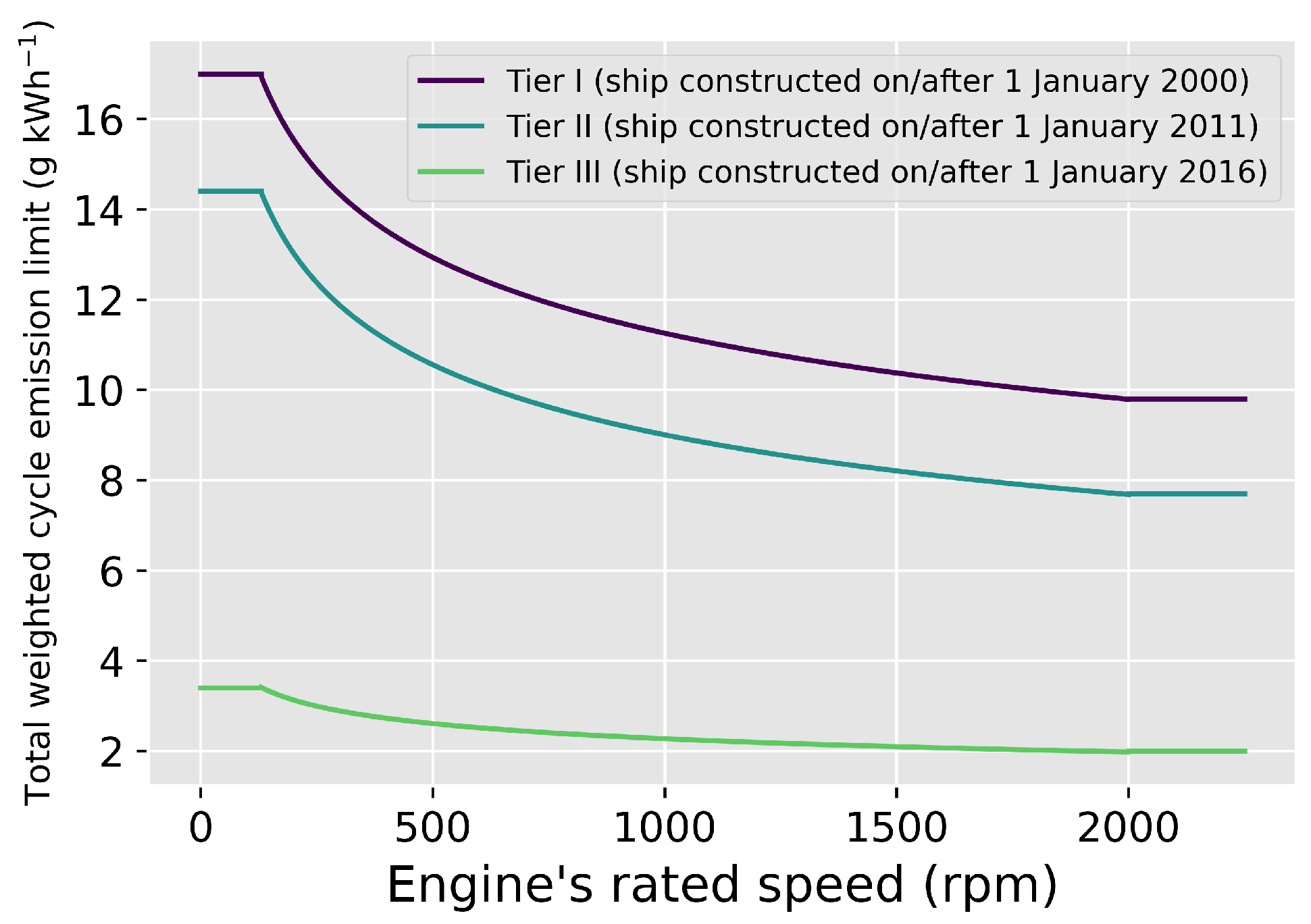
Nitrogen dioxide (NO2) is a highly reactive trace gas that plays a crucial role in both public health problems and environmental pollution. It is primarily released into the air through fuel combustion [1,2,3]. The presence of NO2 in the atmosphere exacerbates respiratory symptoms in humans and causes environmental pollution through acid rain [3,4,5]. Shipping is a significant contributor to global air pollution, responsible for about 15% of global NOx emissions [6,7], particularly in areas near coastlines [8]. As a response, governments and non-governmental organizations are striving to reduce anthropogenic NO2 emissions from ships. The International Maritime Organization (IMO) has enforced regulations on the emission of nitrogen oxides (NOx) from newly built vessels to comply with stricter standards [9]. Ships must comply with NOx emission regulations when entering NOx emission control areas, and stricter regulations are imposed on newer ships to further reduce marine NOx emissions as shown in Figure 1.
Governments and international organizations have urgently called for a reduction in shipping emissions [10,11,12]. To achieve this reduction, monitoring of shipping emissions is essential. Recent studies have attempted to track NO2 ship emissions through remote sensing with the advent of technology such as the TROPOspheric Monitoring Instrument (TROPOMI) on board the Copernicus Sentinel-5 Precursor satellite, which provides high sensitivity and smaller ground sampling [13]. One study has shown the possibility of visually tracing ships based on their exhaust as recorded by TROPOMI [14]. However, this approach requires continual human effort to review numerous remote sensing images daily, making it susceptible to human error and subjectivity. Instead, selectively investigating a region identified as suspicious of particularly high structural bias in terms of NO2 concentration can be helpful for effective regulation implementation.
To address this issue, we propose a systematic approach to separate shipping signatures from background values in the NO2 columns. Our approach includes spatio-temporal data preprocessing and unsupervised clustering of NO2 columns, enhancing the interpretation and visualization of observational TROPOMI data for busy shipping routes. The purpose of this paper is to pinpoint relative hot spots and trends of NO2 concentration in the shipping route, not the absolute NO2 emission estimation. We conducted our research during the period from 5 December 2018 to 10 November 2021 on three regions of interest with considerably higher NO2 emissions [15]: the Mediterranean Sea, the Red Sea, and the Indian Ocean. We verified the validity of our approach by comparing the results with publicly available ship track count estimates [16] and a real-world global logistics index [17] to ensure that the clustering result reflects the shipping patterns and economic trends. Our results can be used to determine whether the amount of NOx emissions is consistent with the expected level from all the ships in a given shipping route or whether there is a structural bias in the NOx emissions.
In Section 2, we present a comprehensive review of related works on tracking NO2 emissions from ships. The current state of the dataset used in this paper is checked in Section 3. In Section 4, we propose the research model and its structure. The methodology of the research model is explored in detail in Section 5. Section 6 presents the results obtained from the methodology applied to the dataset and validates the results by collating them with a real-world global logistics index. Finally, we discuss our findings in Section 7.
2. Related Works
Researchers have attempted to measure ship NOx emissions by directly analyzing ship plumes using mobile and/or stationary instruments. Berg et al. [18] conducted flight transects across ship plumes to verify the feasibility of airborne optical measurements using reflected skylight from the water surface as the light source. Alföldy et al. [19] established an empirical relationship between engine operating conditions and NO2 emission factors from ship plumes at the entry to the port of Rotterdam. Pirjola et al. [20] observed a significant decrease in NOx emissions from ships equipped with selective catalytic reduction, with the help of a mobile laboratory van. Lööv et al. [21] measured NO2 emissions from ships by extracting ship plumes using a sonde instrument, suggesting that optical remote sensing of NO2 emissions from ships can provide reliable estimates compared to direct measurements.
After the successful verification of optical remote sensing technology in ship emission measurements, further studies have established a connection between satellite observational data and ship emissions. Richter et al. [22] visualized NO2 emissions along busy shipping routes, although those observations with poor satellite resolution may be dominated by an aged ship plume. Boersma et al. [23] discovered a noticeable drop in average NOx emissions in Europe via satellite measurements achieved by the implementation of seafaring ships that operate at slow speed. Georgoulias et al. [14] proposed that one can detect individual ship emissions from the TROPOMI NO2 column density by comparing them with automatic identification system (AIS) data. Riess et al. [24] visualized the correlation of TROPOMI NO2 column density with shipping emissions over European shipping lanes, displaying the impact of coronavirus disease 2019 (COVID-19) lockdown measures observed in AIS data.
Despite having the best resolution, TROPOMI measurements are not exempt from spatial dependence. The first law of geography states that “everything is related to everything else, but near things are more related than distant things” [25]. In other words, georeferenced observations tend to have a high correlation with their neighboring observations, known as spatial autocorrelation or spatial heterogeneity. Generally, a spatial dataset is not completely independently distributed but rather displays information redundancy [26]. Georeferenced remote sensing data can have large relative uncertainties in individual measurements due to spatial variations in NO2 profiles and surface albedo [27]. Therefore, reducing information redundancy before satellite data analysis is important.
To the best of our knowledge, most of the previous analyses using TROPOMI measurements have not properly handled spatial autocorrelation. Most researchers deal with spatial data by oversampling, which is a technique of collecting numerous data from the same geographic coordinates over time and then averaging them. This technique can also be referred to as the process of averaging Level 2 data over a long period to obtain a Level 3 grid that is significantly finer than the Level 2 pixels [28]. Several studies have shown the effectiveness of oversampling in enhancing resolution to resolve complex spatial heterogeneity [29,30,31,32,33]. This may be convenient in creating representative values for given geographic coordinates, but temporal oversampling may have averaged out the daily spatial heterogeneity [34]. Taking into account the first law of geography, a single daily event of NO2 emission exerts spatial influence on the NO2 concentration level of neighbors on the same day. In other words, the local spatial autocorrelation is the main driver of spatial heterogeneity on daily TROPOMI measurement. Recently, a study demonstrated an image processing technique that enhances the TROPOMI image quality by reducing background noise using spatial association statistics [35,36]. However, this method has not yet been generalized to other regions and multiple time periods to reflect the real-world business cycle.
In general, machine learning models require well-prepared data for accurate predictions [37]. Therefore, data preprocessing can significantly impact the performance of a predictive model [38]. In this paper, we demonstrate that our methodology can properly identify shipping routes when the processed spatio-temporal TROPOMI data are utilized. The main contributions of our research are as follows:
- We demonstrate an unsupervised method to identify shipping emissions using NO2 column density data without the true ship location information (e.g., AIS data) provided prior to the analysis.
- We propose guidelines for reflecting spatial and temporal heterogeneity when analyzing shipping emissions using remote sensing data.
- We demonstrate the efficacy of our method in identifying shipping emissions by validating it with real-world data of spatial ship track location and temporal economic trend data.
3. Research Scheme
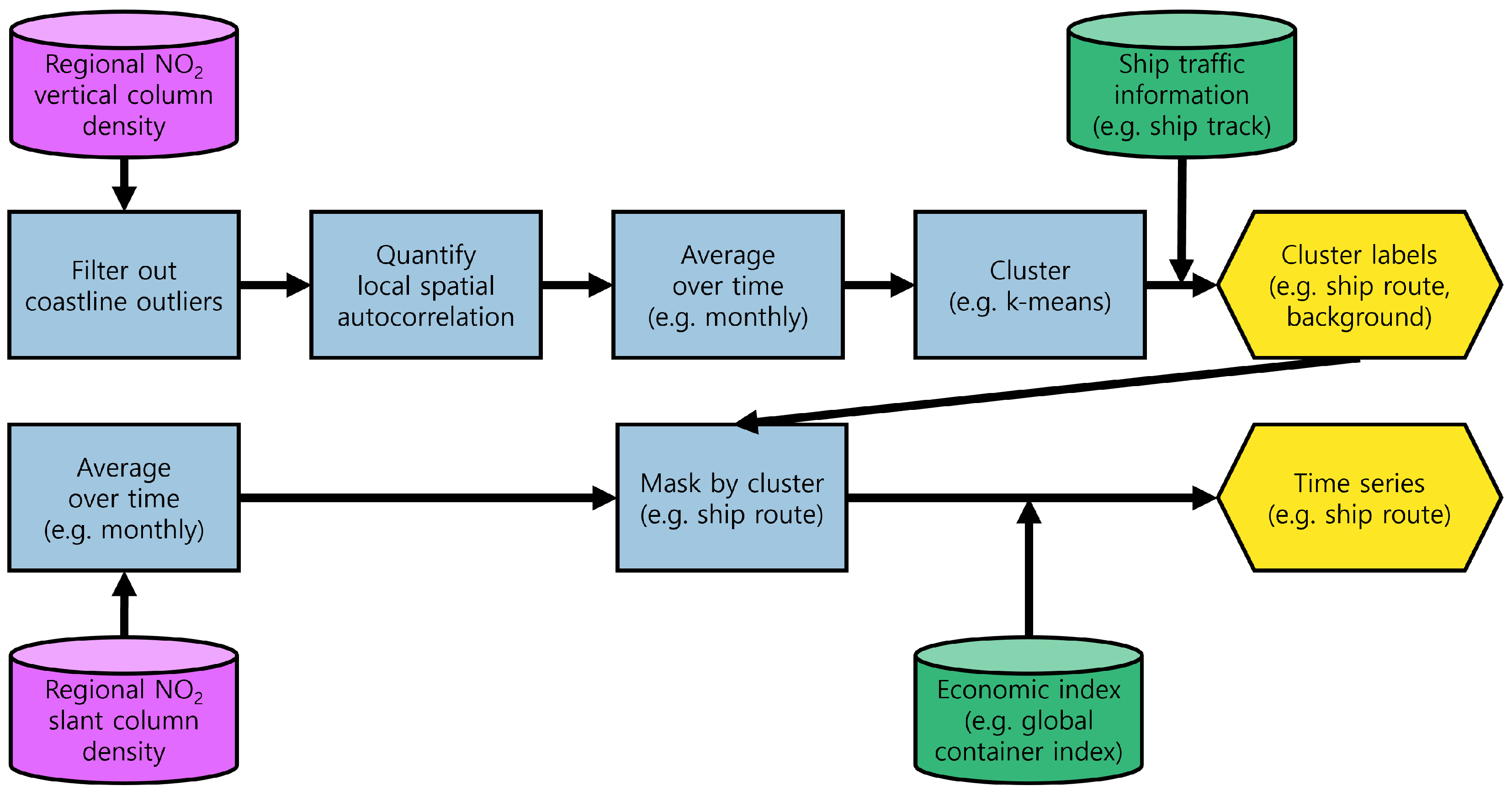
In this section, we provide an overview of the systematic approach to identify shipping emission activities. To aid comprehension, we illustrate the proposed approach as a schematic representation in Figure 2.
First, we propose using NO2 column density as a proxy for shipping emissions in the open sea. Since NO2 is the dominant form of NOx emitted from aged ship plumes in atmospheric air [22,39,40], we can consider the NO2 concentration in ship plumes as a proxy for the total amount of ship emissions. Provided there is no stationary anthropogenic emission stronger than shipping, which we assume to be the case, the distinctively high NO2 column density in the open sea primarily results from cumulative shipping emission activities, namely the cumulative NO2 concentration along the shipping route. Consequently, we suggest using the average level of cumulative NO2 column density as a proxy for shipping frequency.
Second, we present a method for handling spatial autocorrelation. As TROPOMI data are inherently georeferenced data, we must deal with spatial dependence for each daily image. Therefore, we need to reduce the interdependence among spatial data, firstly by removing outflow from the land near the coastline, and then quantifying the spatial autocorrelation of the NO2 column density.
Third, we demonstrate how to partition the NO2 column density by k-means clustering of spatially processed and temporally oversampled data. The clustering yields labels that the user can annotate with interpretations, such as the shipping route with the highest average NO2 column density.
Finally, we validate the outcome by visualizing spatially and quantifying how TROPOMI NO2-based clusters correlate with ship tracks from a publicly available cumulative ship track dataset [16]. We further validate the result by plotting the time series of TROPOMI NO2 column density and the global economic index to show how the NO2 column density trend for shipping routes is similar to the real-world container throughput trend [17].
4. Materials
4.1. TROPOMI NO2 Datasets
In this study, we demonstrate a systematic approach to identify shipping emission activities using remote sensing instruments. Specifically, we utilize the remotely sensed NO2 column density retrieved by TROPOMI, a satellite instrument that has gained attention due to its unprecedented high resolution and sensitivity.
Compared to its predecessors like Global Ozone Monitoring Experiment [41] and Ozone Monitoring Instrument [42], TROPOMI on board the Sentinel-5 Precursor satellite [13] has a much higher sensitivity and smaller ground sampling technology. With a resolution of near nadir, which has been improved to as of August 2019 [43], and can be further enhanced to by oversampling [29,30,31,32,33], TROPOMI can be used for mapping and tracking shipping activities [14].
From the TROPOMI NO2 product, we make use of two datasets: (1) the NO2 tropospheric vertical column density (VCD) and (2) the NO2 tropospheric slant column density (SCD), retrieved using differential optical absorption spectroscopy [44,45,46]. Specifically, we have used the near real-time (NRTI) Level 2 TROPOMI data and then processed this with our own in-house Level 3 processor. The data are stored in the georeferenced Network Common Data Form format [47], with four dimensions: (1) latitude (unit: decimal degree); (2) longitude (unit: decimal degree); (3) time (unit: day); and (4) NO2 column density (unit: mol m).
To ensure the reliability of the data, we consult the TROPOMI Algorithm Theoretical Basis Document [43] and select NO2 column density data based on the following criteria: quality assurance value (qa_value) , cloud fraction , and viewing zenith angle °. Regarding the viewing zenith angle, the value of ° is arbitrary, but this should be enough if the purpose of the filter is to filter our poorer quality data. These criteria were recommended at the time of data retrieval to include good-quality data and moderately filter out data with errors in retrievals, to gather data from a clear sky, and ensure data reliability, respectively. Regarding the qa_value in particular, we used qa_value as it is a useful criterion where the averaging kernels are used [48]. The proposed method suffices this condition as we implement spatial processing of NO2 column density data.
It is worth noting that the purpose of this paper is to verify the validity of the statistical analysis on trends and changes of the NO2 concentrations rather than to estimate the absolute amount of emission. Therefore, we choose to include lower-quality data to demonstrate the validity and robustness of the proposed method against such data. After selecting the quality of measurement, we regrid and average the data. Specifically, we interpolate all irregularly gridded Level 2 data on a regular lattice defined in the World Geodetic System 1984 (WGS84) and time-average the data for the same measurement pixel available with valid data from different points in time on the same day.
To promote the generalizability of the proposed method, we analyzed TROPOMI NO2 column density data from multiple regions over an extended period. Table 1 shows the properties of the datasets used in the paper, including the spatial and temporal coverage of each dataset.
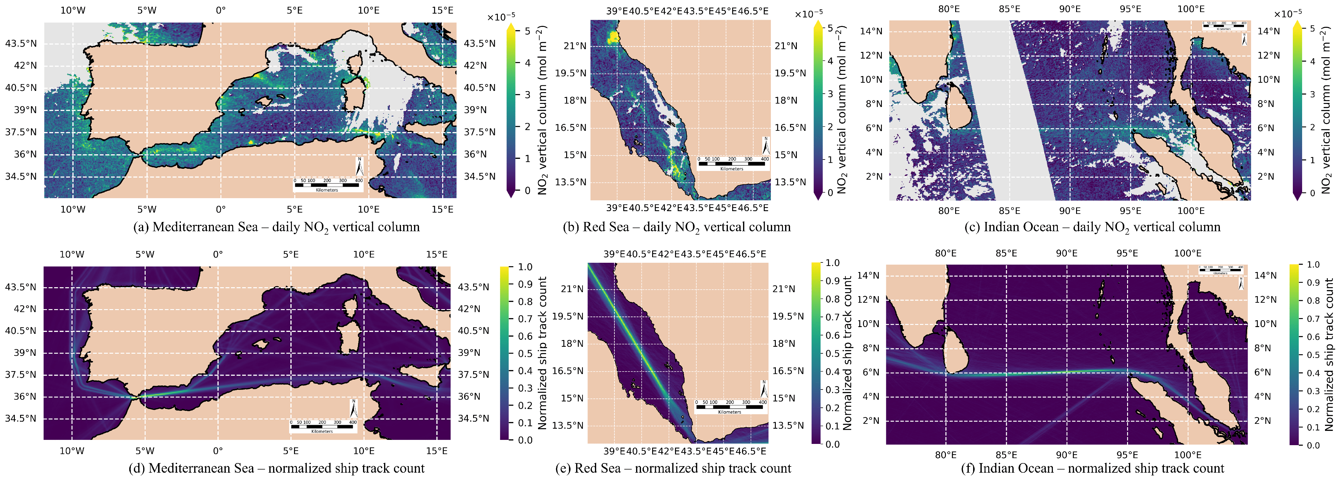
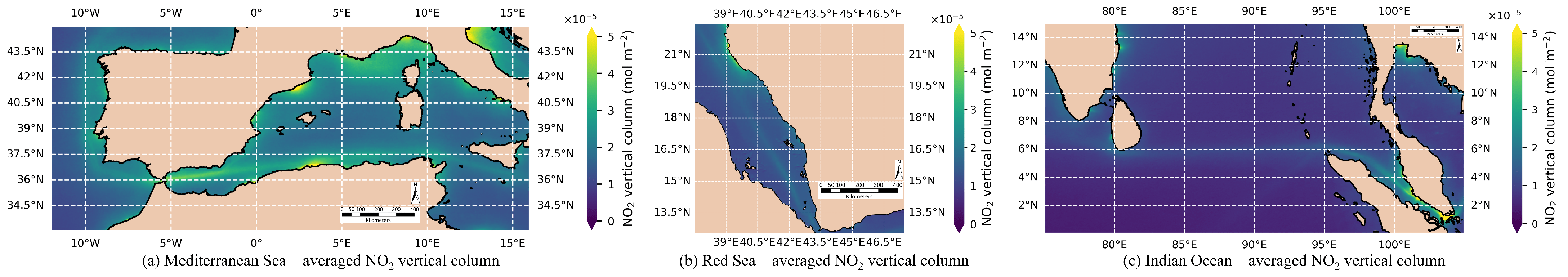
In terms of spatial coverage, we selected three of the busiest shipping routes in the world, as illustrated in Figure 3. The dataset covers the following geographic regions with bounding WGS84 coordinates in decimal degrees as shown in Table 1. The equirectangular-regridded NO2 column density data points have the resolution of a square pixel with a sampling rate of 0.03125 degrees in both latitude and longitude. Thus, a pixel in the regridded map represents the NO2 column density within a quadrangle of approximately at the equator, where the Earth’s circumference is approximately 40,075 km long. The pixel width of the regridded map decreases as the latitude of the pixel moves away from the equator. Consequently, there is a slight oversampling in the regridded map as the latitude moves away from the equator.
In terms of temporal coverage, we selected the time period covering before and after the outbreak of the COVID-19 pandemic as shown in Table 1. For each day, there is a single NO2 column density per pixel, derived from the TROPOMI measurement at the 13:30 overpass local solar time. In other words, the dataset has a temporal coverage of a total of 1072 days with one measurement per day.
Formally speaking, the regridded TROPOMI NO2 column density datasets serve as the original input data X defined in a cubic lattice space of latitude, longitude, and time. We define as a square lattice that consists of all original input data values at time t. Within , we define a single entry of as , referenced over coordinates at time .
4.2. Spatio-Temporal Validation
To validate the proposed method for identifying shipping emissions, we imported two open-source datasets:
- Spatially, we brought in a ship track count data [16] to verify that our results match real-world ship track data. Each geographic coordinate has vessel location information representing the total counts of ship tracks recorded in the data collection period. We used the normalized form of the total ship track counts per region. Lastly, the normalized counts were regridded on the same coordinates as the TROPOMI NO2 column density.
- Temporally, we brought in a global container throughput index [17] to demonstrate that our results reflect the global business cycle of shipping volume. This index is an estimate of global container throughput, representing about 60% of the global trade volume via shipment collected from a total of 89 international ports from December 2018 to November 2021. Since our regions of interest lie along busy shipping routes connecting Europe and Asia, the trend of the global trade volume should be reflected in the trend of emission concentrations in these regions.
In general, the spatial validation dataset serves as the true value of the normalized ship track counts considered over coordinates i. The temporal validation dataset serves as the true value of the global container throughput index considered over coordinates i.
5. Methods
5.1. Data Preprocessing
5.1.1. Near-Coast Removal
We begin by removing spatially irrelevant NO2 data from inland emission sources. The NO2 column densities show relatively large uncertainties near the coastline and localized sources such as power plants [27]. Therefore, we need to remove not only the NO2 data from inland emission sources but also from those near the coastline, as these are most likely to be outlier values.
Inland data must be removed since the NO2 signature will be dominated by stationary inland emission sources. To remove data from irrelevant inland emission sources, we first mask the data over land. This can be accomplished by masking with the freely available Natural Earth 1:10 m physical vector map of land polygons, including major islands [49].
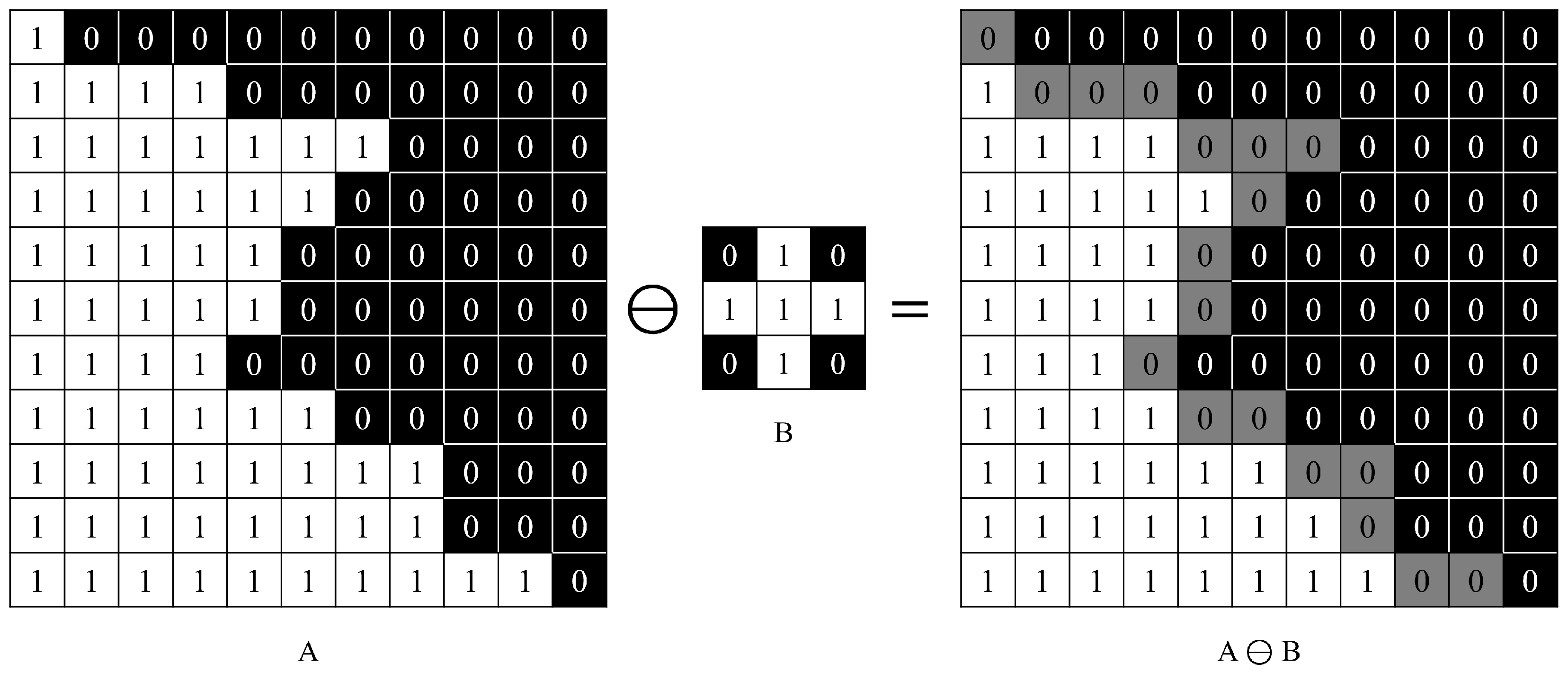
Since NO2 travels in the atmosphere via the wind, the NO2 data over near-coast oceans are highly influenced by spillover from inland emission sources and must be treated as outliers. Here, we presume the width of the near-coast oceanic region to be about 70 km away from the coastline. The near-coast ocean region is removed using morphological binary erosion [50]. Binary erosion can be defined as the binary morphological operation (⊖) between the original image of an image in a Euclidean space E, operand , and the shape parameter or the kernel, operand , such that
where denotes a translation vector of B to probe across A, and is a translation of B to z. If can be contained in A, then z is said to belong to the erosion . z has a value of one when it belongs to the erosion , and zero otherwise. A visual example of the binary erosion operation is shown in Figure A2. To erode the NO2 column density near the coast, we use a binary Gauss circular kernel, illustrated in Figure A3, with a radius of twenty pixels, or equivalently, a geodetic distance of 70 km. In other words, k and l are set to twenty for the erosion of near-coast pixels. Note that the choice of k and l are arbitrary, and they are fixed to twenty to promote the simplicity of the proposed method. A visual example of near-coast removal is shown in Figure A4. By removing data near the coast, most of the data with large NO2 column density with almost no ship track are removed, as displayed in Figure A5. After the removal of near-coast pixels, we obtain a NO2 column density that corresponds better with open-sea ship tracks.
5.1.2. Spatial Data Preprocessing
Most of the time, spatial data contain redundant information [26]. In other words, geographical data do not typically represent independently generated incidents, but instead reflect a sum of spatial spillover influences exerted by neighboring data [51,52]. For example, remotely sensed gas leakage images [53] show that pixels near the emission source tend to have higher readings than those farther away. As mentioned earlier, NO2 emission events have a spatial spillover effect on the NO2 levels of neighboring areas. This effect is much larger for local pockets of spatial dependence [54,55] near the anthropogenic NO2 source [56,57].
Traditional regression models, such as the least squares method, assume independently distributed data, which may not hold true for spatial data [51]. Additionally, the least squares method produces distorted results with outliers, as they dominate the sum of squares calculation [58]. Thus, to resolve the information redundancy of spatial data, we quantify the original NO2 column density into a local indicator of spatial autocorrelation (LISA). Two popular LISA metrics are Getis-Ord [54,59] and local Moran’s I [55].
In this study, we use the statistic because we aim to identify the hot and cold spots of NO2 concentration to identify the shipping signature. Hot (or cold) spots are the specific spatial clusters of high (or low) values, with zero being the division criterion. Although local Moran’s I is a popular LISA metric that can quantify the statistical significance of spatial heterogeneity, it only represents the significance of the spatial heterogeneity and not whether it is a hot or cold spot. Using local Moran’s I may assign high values to both shipping and the background signature if both are significantly spatially heterogeneous. In contrast, we want to clearly distinguish the shipping signature from the background and not categorize them together with the same statistical significance. Therefore, we select as the spatial data preprocessing tool to generate both hot and cold spots.
was originally introduced by Getis and Ord [54] as a statistic quantifying the spatial autocorrelation of a local pocket near a target data point. First, we define the target data point as with known coordinates i at time t, using the same notation as in Section 4. Then, measured at is defined as follows:
where denotes the symmetric binary spatial weight matrix between and , whose elements are one when is within distance d from data and zero otherwise (j may equal i). Typically, d is chosen as a squared distance in Euclidean space.
Later in [59], the statistic is revised into a standardized statistic, denoted here as . measured at is defined as follows:
where denotes the sample mean of all measurements in , s denotes the sample standard deviation of all measurements in , and N denotes the sample size.
A drawback of Equation (3) is the expensive computation of the weight matrix, especially for remote sensing data. As remote sensing data generally have a large number of data entries, the observations are usually non-zero, unless filtered out by a low quality-assurance value or a high cloud fraction. In conventional spatial data analytics tools such as ArcGIS [60], the spatial weight matrix for every target region i is constructed for all neighbors within d. Although it utilizes a sparse spatial methodology to save storage space and reduce execution time [61], selecting a high number of neighbors can cause memory issues [60].
Therefore, we modify the calculation of the spatial weight matrix with convolution filtering [62], one of the most widely used image processing algorithms in pattern recognition and computer vision. By replacing the weight matrix with its convolution, we obtain the same result without the expensive computation of the spatial weight matrix. The finite discrete convolution operation between the kernel matrix and the target intensity matrix is defined as follows:
where k denotes the vertical lattice tick, l denotes the horizontal lattice tick, and and are the coordinates of I for and . We refer to the element of at coordinates i as . When the convolution operation encounters an empty cell from I, such as the cell beyond the boundary of I or values filtered out for quality, the operation regards such an entry as empty and calculates using other available data. If none of the entries are available, then the operation returns the target data point as empty.
Equation (4) represents the mathematical model for performing convolution operations between the kernel matrix and target intensity matrix. The kernel matrix K can be designed to detect specific features in an image, such as edges, corners, or other relevant patterns. The convolution operation convolves the target intensity matrix I with the kernel matrix K to produce an output matrix , which highlights the detected features in the image.
Using the aforementioned convolution operation, we propose a modified version of the statistic, denoted as , which measures the spatial autocorrelation of the local pocket near a target data using convolution filtering. The at coordinates i between the kernel K and input intensity dataset at time t, , is defined as follows:
where , , and denote matrices of size , , and , respectively. The kernel size parameters are generally selected as and to compute the local spatial autocorrelation. While arbitrary size is allowed for the kernel, we use a square kernel matrix of size for convenience. Note that if even numbers of rows and columns are selected, then the kernel size becomes . For computation, we use a binary Gauss circular kernel with a radius of 5 pixels, or equivalently, 17 km geodetic distance. In other words, k and l are set as five for the computation of spatial autocorrelation using convolution. Note that the choice of k and l are arbitrary, and they are fixed to five to promote the simplicity of the proposed method. By such computation, we obtain the spatially resolved statistic of the NO2 column density, as visualized in Figure A6.
5.1.3. Temporal Data Preprocessing
After resolving the spatial autocorrelation, we can proceed to the next step of temporal data preprocessing to further enhance the resolution. As oversampling is a proven technique to achieve finer resolution [29,30,31,32,33], we can average the NO2 column density over time. Several previous studies have conducted research on the monthly averaged TROPOMI NO2 column density. However, we strongly believe that the location of a busy shipping route does not vary month by month, because the shortest shipping path, which is the most economic route [63], is already determined and is likely to remain constant for years. Therefore, we extend the oversampling window over the entire test period as shown in Table 1 to obtain a single shipping route that reflects the shipping patterns over the entire period. Conventional oversampling is equivalent to taking the sample mean of the NO2 column density at coordinates i over time .
Instead of conventional oversampling, we propose to first resolve the spatial heterogeneity. Here, we oversample from instead of the original input data:
As mentioned earlier, oversampling may exclude daily events with overshooting NO2 column density. While oversampling is effective in suppressing noise signatures [28], it may underestimate unexpectedly high peaks of NO2 emission from non-compliant ships. Despite this drawback, oversampling retains its spatial significance throughout the test period as it captures constant ship activities around the busy shipping route. Therefore, the oversampling technique does not compromise our aim of retaining shipping route information from the TROPOMI NO2 column density.
5.2. Clustering
Partitioning can aid human interpretation by assigning labels to each pixel while considering the column density values of neighboring pixels. As TROPOMI datasets contain continuous numeric data, it is important to distinguish which values are relatively high in comparison to other values in the region of interest. We partition the spatio-temporally resolved TROPOMI datasets using a clustering algorithm to obtain cluster labels for the NO2 column density. Although the approach is not dependent on any specific clustering algorithm, we demonstrate the approach using the k-means clustering algorithm, an unsupervised classification of grouping patterns into k clusters. The original concept of k-means clustering was introduced by Steinhaus [64], and the full algorithm was developed by researchers such as Lloyd [65] and MacQueen [66] in the mid-20th century. Despite its age, k-means clustering remains one of the most commonly used clustering techniques due to its simplicity and speed [67]. We adopt the k-means clustering algorithm suggested by Lloyd [65] to partition the spatio-temporally resolved NO2 column density using squared distance as the dissimilarity measure. We define the k-means clustering algorithm as an optimization problem of finding k centroids that minimize the within-cluster sum of squares (WCSS) as follows:
where denotes the centroid of the jth cluster , and denotes a weight of value one if belongs to and zero otherwise.
One caveat of using the k-means clustering algorithm is that the centroids of produced clusters are only meaningful when the cluster shape is roughly globular [68]. In our case, we aim to identify shipping emissions, where ships travel along linear routes and emit exhaust while sailing. As a result, the ship exhaust detected by remote sensing tends to follow a linear path and form an elongated shape, rather than a globular one. Therefore, we cannot simply cluster data that exhibit spatial spillover effects.
To properly handle spatially autocorrelated data such as TROPOMI images, we propose quantizing the NO2 column density as a scalar by collapsing the spatial dimension. This is because the collapsed data no longer depend on the spatial parametric setting, and scalar quantized data can be georeferenced back to their original coordinates. Thus, clustering will preserve the non-parametric spatial structure, such as an elongated shape, even after clustering. We use Lloyd’s algorithm in its original format of scalar quantization, where georeference information is collapsed and all data are sorted in terms of the NO2 column density level. Our objective is to find a scalar quantizer that partitions the data into k levels. Scalar quantization can be performed by applying k-means clustering to the one-dimensional NO2 column density.
Another caveat is the dependency of the algorithm on the initial assignment of centroids. This issue is often mitigated by performing multiple trials of k-means clustering and optimizing the results by selecting the best outcome. To this end, we employed k-means++ [69], an improved initialization technique with randomized seeding.
A final caveat is that the performance of k-means clustering highly depends on a predetermined number of clusters. As for the dependency on the predetermined cluster number, it can be solved analytically by choosing an optimal number of clusters. While there are numerous techniques for determining the optimal number of clusters, we demonstrate one of the most common methods: the elbow method [70]. This method chooses the optimal number of clusters where the elbow of the WCSS curve is located. We select the elbow of the WCSS curve of cluster k, denoted as , by performing k-means clustering over a set range of k. Formally, we define the distortion as follows:
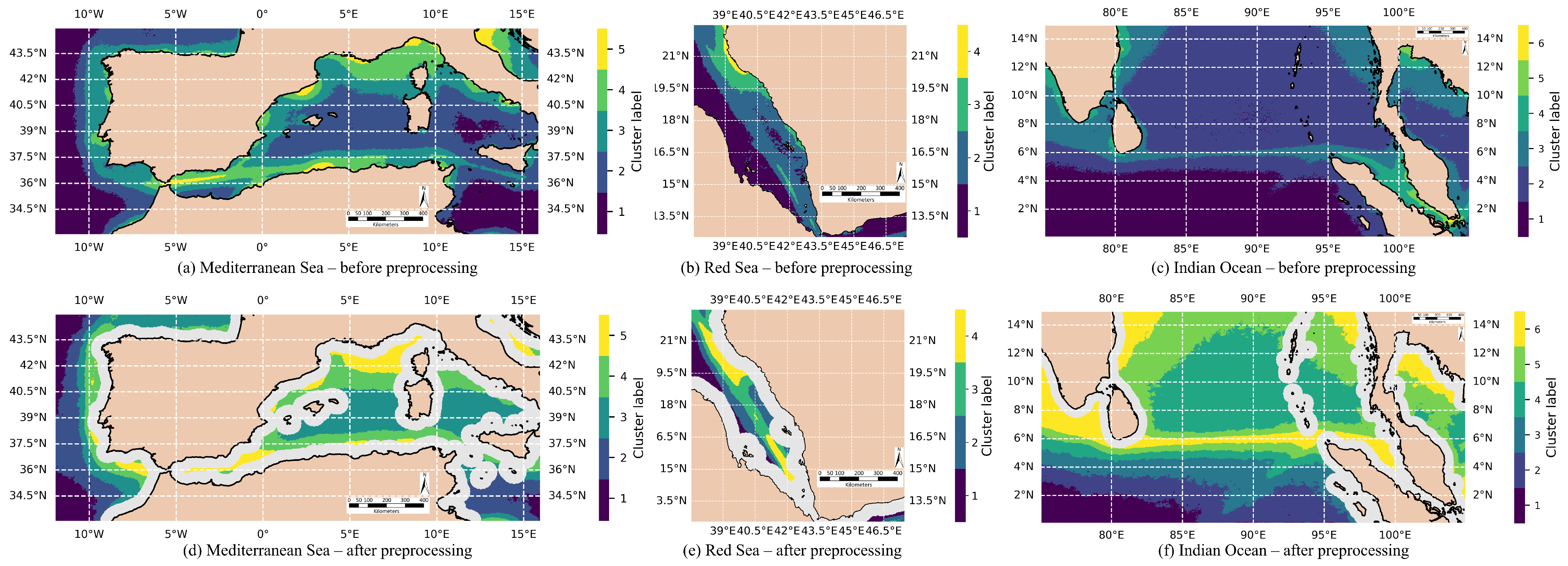
where any pair of observations and belongs to the same cluster with observations, and denotes the centroid of . The elbow point is defined as the point where the k-means clustering achieves the best fit or where the variance is explained as much as possible before overfitting occurs. We assume that the elbow point is located at the largest difference between the original curve and its reference line, as shown in Figure A7. In other words, it is a maximization problem of the WCSS difference given a set of the number of clusters. We calculate the optimal number of clusters using the elbow method, which is five for the Mediterranean Sea, four for the Red Sea, and six for the Indian Ocean. The cluster labels are sorted in ascending order of the spatially resolved centroid of NO2 column density using . Finally, the shipping signature can be identified as the cluster with the highest NO2 column density on average, by integrating spatio-temporal data preprocessing and clustering techniques.
5.3. Quantification of Spatial and Temporal Correlation
For the quantification of spatial and temporal data preprocessing, we use the sample Pearson correlation coefficient r as a model assessment criterion. The bivariate sample Pearson correlation between two data points u and v is defined as follows:
This Pearson correlation is used to calculate either spatial correlation or temporal correlation between two data.
6. Results and Discussion
6.1. Validation of Spatial Data Preprocessing
In this section, we validate the proposed methodology by demonstrating the increased correspondence of spatio-temporally preprocessed NO2 column density with publicly available shipping frequency patterns and economic trends, compared to the original column density and clustered column density without spatio-temporal data preprocessing.
First, we calculate the spatial correlation between the clustering results of the NO2 column density and the normalized ship track counts. The spatial correlation is calculated by solving Equation (9) between the NO2 column data, such as the original or clustered data, and the validation data, which are the normalized ship track counts. We assume that the true shipping frequency can be estimated by the ship track counts dataset [16]. Such an assumption is based on a strong belief that the location of the shipping route remains constant for years due to the ship operators’ tendency to travel along the shortest path, as explained in Section 5.1.3.
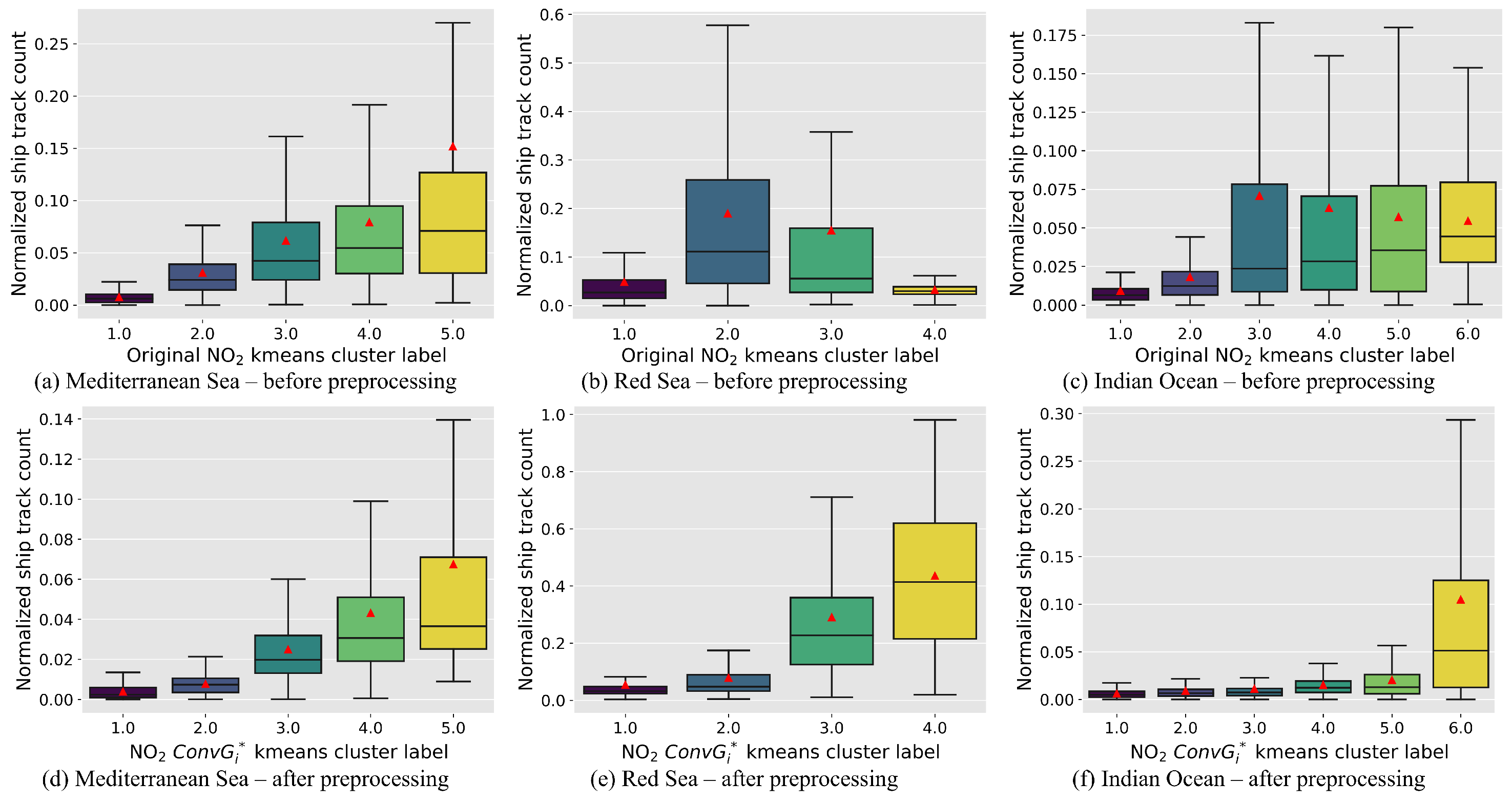
We will now compare the two clustering results: one before resolving spatial autocorrelation by spatial data preprocessing (Figure 4a–c), and the other after resolving it (Figure 4d–f). The cluster label is a sorted representation of the average NO2 column level within the cluster. As explained in Section 5.2, the cluster labels are sorted in terms of the NO2 column level of cluster centroid, for instance yielding from 1 to 5 in the Mediterranean Sea. Each cluster label may have its own interpretation, and we assign meanings to the highest and the lowest as the cluster with the highest NO2 concentration and the background cluster or the reference cluster. Since our proposed method aims towards the systematic identification of shipping emissions, it will be easier if we could assume that the cluster with the highest NO2 concentration corresponds to the shipping route cluster.
It is non-trivial to manually assign the shipping route label to any cluster in between, since the number of clusters is subject to change per region and such interpretation is prone to human subjectivity. Before preprocessing, the cluster labels with higher labels correspond to the coordinates with relatively high average NO2 emission concentration levels compared to other clusters. Since it is not spatially preprocessed, the highest may not correspond to the shipping route, but rather the NO2 emissions from the land. Such behavior is shown in the boxplots of Figure 5a–c, as the clusters with the highest labels do not always have the highest ship track counts. It is therefore a difficult task before preprocessing to correctly interpret which cluster label is the shipping route.
We propose to overcome this non-triviality in shipping route identification by spatially preprocessing the NO2 concentration data and relying on the systematic approach to identify the shipping route as the highest cluster label. After spatial data preprocessing, higher cluster labels correspond to higher ship track counts, indicating that the preprocessed clusters better reflect the shipping density pattern. Spatial data preprocessing particularly enhances the meaning of the highest cluster label in the Red Sea and in the Indian Ocean, as the clusters before preprocessing may have been largely influenced by spatial spillover and inland emission activities. The changes from spatial preprocessing are apparent, as the cluster shape of the highest cluster labels visually correspond to the major busy shipping routes in test regions of Figure 4.
Figure 5 demonstrates the effectiveness of the operation by showing the proportional relationship between cluster labels and ship track ratios. The results show that spatial data preprocessing improves the correspondence of NO2 column density to the shipping pattern, as it preserves the increasing trend of normalized ship track counts. We intend to cluster the NO2 column density in proportion to ship track counts, so the cluster label with the highest number should represent the largest amount of ship track counts. In particular, the cluster labels of the Red Sea recover their monotonicity after spatial preprocessing, as near-coast removal excludes the land-based emission influence from the coastal regions.
The effectiveness of spatial data preprocessing lies in the design of the k-means algorithm. Since the algorithm calculates WCSS generally based on a distance metric, the k-means clustering algorithm is sensitive to outliers. By removing the information redundancy and the outflow effect from coastal region activities via spatial data preprocessing, we see an overall improvement in clustering performance as shown in Table 2. As a result of spatial preprocessing, the clustered NO2 data better represent the relatively higher NO2 from shipping in the open sea, both visually and quantitatively.
6.2. Validation of Temporal Data Preprocessing
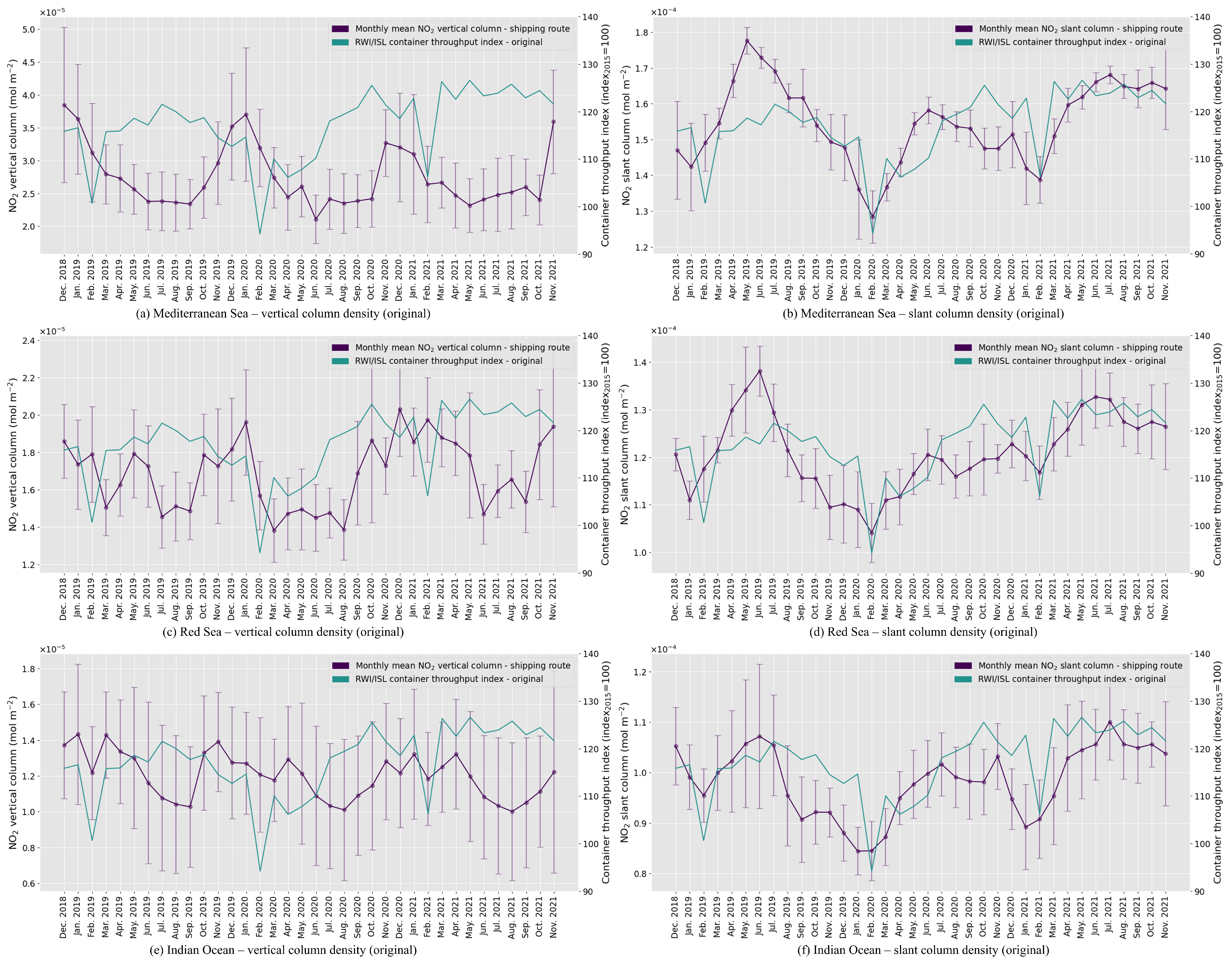
In addition to verifying spatial correspondence with ship tracks, we validate the proposed methodology by demonstrating how well the shipping route cluster reflects the global business cycle. Demand for shipping transportation is a key determinant of global economic activity [71,72]; therefore, the estimated shipping route should resemble the global business cycle. Researchers have found that global shipping throughput data reflect the global economic recession due to the COVID-19 lockdown measures [73,74,75]. We validate the results by comparing the monthly averages of NO2 column density in the shipping route over the entire time period as shown in Table 1. Here, we assume that the NO2 data point belongs to the shipping route cluster with the highest mean NO2 column density. To temporally validate our results, we compute the correlation between the NO2 column density of the shipping route and the global container throughput index for the same time window. The temporal correlation is calculated using Equation (9) between the monthly averaged NO2 column density within the shipping cluster and the monthly index of global container throughput. The global container throughput data are available online as the Rheinisch-Westfälisches Institut für Wirtschaftsforschung and the Institute of Shipping Economics and Logistics (RWI/ISL) Container Throughput Index [17].
Figure 6 shows the monthly averaged NO2 column density of the shipping route matching the monthly trend of the global logistics volume. Its deseasonalized version is shown in Figure A8 shows the seasonally adjusted NO2 column density, using the classical seasonal decomposition [76]. Particularly in early 2020 and early 2021, a sudden drop is observed in both the NO2 trend and the container throughput trend, followed by recovery back to the previous level. Table 3 shows the temporal correlation between the and time series plotted in Figure 6. The yearly differences from 2019 to 2021 are displayed in Table A2 with VCD and Table A3 with SCD.
In addition, we have conducted another experiment using Copernicus Atmosphere Monitoring Service (CAMS) global reanalysis ECMWF Atmospheric Composition 4 (EAC4) dataset of atmospheric composition [77]. Figure A9 shows that CAMS data on the shipping route show a similar trend with NO2 tropospheric VCD on the shipping route. Note that the trend of CAMS data matches with NO2 tropospheric VCD, which is used for spatial preprocessing of NO2 data and yielding clusters. This result shows that the quality of our approach to processing TROPOMI NO2 data is comparable to CAMS global reanalysis (EAC4) result on the shipping route.
We observe that the NO2 tropospheric SCD can better represent the global shipping density and economic trends. As shown in Table 3, the temporal correlation between the NO2 column and the global container throughput index is much better when it is compared with NO2 tropospheric SCD. While we propose using the NO2 tropospheric VCD in clustering, we suggest also using the NO2 tropospheric SCD when matching the global economic index due to the following reasons.
The TROPOMI VCD has been known to be sensitive to the a priori estimate of the NO2 profile shape [78]. This is because the assumptions made during the a priori calculation of the air mass factor may not hold in regions with high pollution levels [79]. In particular, there is a high level of structural uncertainty in air mass factor calculation over regions with high NO2 pollution [80].
Filtering out persistently strong background measurements, such as those caused by high solar radiation during summer and inland anthropogenic emissions, is functional and can help to rule out seasonality and overestimated inland emissions. However, providing the shipping activity locations may be appropriate for certain analyses, but not when the goal is to analyze the measurement itself directly.
Furthermore, it is worth noting that since shipping emissions are consistently high, there is a risk of underestimation. Despite underestimated NO2 concentration in hot spots, we would like to emphasize that our approach is to identify the relative trend of the shipping emission, and not the absolute emission estimation. From the empirical result, we suspect the reason for being able to distinguish the shipping route as the tendency of low NO2 readings remaining low, and very high readings remaining moderately high, such that it is still enough to distinguish the shipping route from the background.
These results are consistent with a previously verified global NO2 inventory for seafaring ships, which showed relatively high NO2 emissions during the summer period compared to the winter period ([81], Figure 4). Therefore, our empirical analysis demonstrates that the monthly trend of the NO2 column density better matches the trend of the global container throughput index.
7. Discussion
This research proposes a method for identifying shipping NO2 emissions by clustering spatio-temporally resolved TROPOMI data. The method partitions geographic coordinates in the open sea into clusters and identifies the cluster with the largest NO2 column density as a shipping route. Experiments were conducted in three selected regions with high shipping density, namely the Mediterranean Sea, the Red Sea, and the Indian Ocean. Each region was spatio-temporally preprocessed and visualized on a respective map. Statistical results show that the proposed method increases the spatial correlation between the TROPOMI NO2 measurement clusters and the ship track counts. Lastly, the TROPOMI NO2 measurements of the highest cluster labels show temporal trends that match with the real-world global throughput index, such as the impact of the COVID-19 lockdown measures on the global trade volume. In summary, the proposed method has demonstrated its effectiveness in identifying shipping routes with high NO2 emissions and in providing insight into the impact of global events on shipping emissions.
Since the purpose of this paper is to identify shipping emissions in the open-sea area, it may require different algorithmic settings to identify emission activities in different environments, e.g., flexible choice of kernel size to filter out near-coast measurements or calculating near-coast shipping emissions with the influence of mixed types of inland emissions. One may need to consider more supporting data when applying this method to coastal area emissions, e.g., wind velocity profiles from land and in situ measurements from coast guard authorities. In addition, the proposed method cannot effectively distinguish the clustered NO2 data by individual vessel types, because the spatial validation is performed at an aggregate NO2 column level.
Through this study, we identified shipping emissions by spotting the trends and changes in the NO2 column level along the shipping route. However, it is yet unknown whether higher NO2 data are also higher in absolute NO2 column data because the spatial preprocessing yields a quantification of showing a central tendency towards the global mean value. In other words, standardizes the NO2 column level which shows the relative position of each data point within its cluster. Therefore, it is uncertain to say that the regions with higher NO2 levels indeed exhibit higher NO2 levels in an absolute sense.
We expect that the proposed method may serve as an exemplary technique to identify anthropogenic emission sources, distinguishing them from the background in future research. While this study focused on open-sea regions, our method can be applied to other regions with trace gas emissions, including inland anthropogenic emission sources. Depending on the purpose of the study, one may skip the land-masking procedure and/or near-coast removal to see the emissions in all available regions, which demonstrates the versatility of the proposed method. In addition, we plan to conduct optimization studies of fixed distances such as fixed geodetic distance used for computation. With the help of more supporting scientific data such as the chemical transport model, we can optimize the spatial correlation based on the atmospheric domain knowledge, such as using geometric air mass factor in VCD calculation to consider its uncertainty or validating the data based on comparisons with high-quality ground-based or other measurements [82]. With validated real-world case studies and scientifically supported results from unsupervised clustering, our method will be effective in environmental governance and regulatory compliance activities related to emission monitoring. The proposed method may be used by port authorities or inspectorates to function as a monitoring tool of a designated region to see the relative changes in aggregate emission level.
Author Contributions
Conceptualization, J.K., R.V. and B.O.; methodology, J.K., M.T.M.E. and J.-S.L.; software, J.K.; validation, J.K., R.V. and B.O.; formal analysis, J.K., M.T.M.E., R.V., B.O. and J.-S.L.; investigation, J.K., R.V. and B.O.; resources, J.K., R.V. and B.O.; data curation, J.K., R.V. and B.O.; writing—original draft preparation, J.K.; writing—review and editing, J.K. and B.O.; visualization, J.K.; supervision, J.K.; project administration, J.K.; funding acquisition, J.K. and J.-S.L. All authors have read and agreed to the published version of the manuscript.
Funding
This research was supported in part by the National Research Foundation of Korea grant funded by the Korean government’s Ministry of Science and ICT (MSIT) grant number 2020R1A5A1019649, in part by the Institute for Information and Communications Technology Planning & Evaluation grant funded by the MSIT grant number 20210002920012002, and in part by the SungKyunKwan University and the BK21 FOUR (Graduate School Innovation) funded by the Ministry of Education (MOE, Korea) and National Research Foundation of Korea (NRF).
Data Availability Statement
The tropospheric NO2 data are publicly available via the Copernicus Sentinel-5 Precursor hub (https://scihub.copernicus.eu/ (accessed on 4 July 2023)). The regridded version of tropospheric NO2 data were provided by Airbus Defence and Space Netherlands by reprocessing tropospheric NO2 data Copernicus Sentinel-5 Precursor hub (version 1.2.0/1.2.2). The regridded tropospheric NO2 data presented in this study are openly available in 4TU.ResearchData repository at https://doi.org/10.4121/16943725 (accessed on 4 July 2023). The analysis software is written in Python 3.9.13 (https://www.python.org (accessed on 4 July 2023)). The code is available at https://github.com/juhuhn/TROPOMI_NO2_clustering (accessed on 4 July 2023).
Acknowledgments
The authors acknowledge the funding sponsors listed above. The authors also acknowledge the 4TU.ResearchData repository for publishing the regridded data.
Conflicts of Interest
The authors declare no conflict of interest.
Abbreviations
The following abbreviations are used in this manuscript:
| NO2 | Nitrogen dioxide |
| NOx | Nitrogen oxides |
| IMO | International Maritime Organization |
| TROPOMI | TROPOspheric Monitoring Instrument |
| AIS | Automatic identification system |
| VCD | Vertical column density |
| SCD | Slant column density |
| COVID-19 | Coronavirus disease 2019 |
| WGS84 | World Geodetic System 1984 |
| LISA | Local indicator of spatial autocorrelation |
| WCSS | Within-cluster sum of squares |
| RWI/ISL | Rheinisch-Westfälisches Institut für Wirtschaftsforschung/Institute of Shipping |
| Economics and Logistics | |
| CAMS | Copernicus Atmosphere Monitoring Service |
| EAC4 | European Centre for Medium-Range Weather Forecasts (ECMWF) |
| Atmospheric Composition 4 |
Appendix A
Figure A1.
Oversampled NO2 tropospheric VCD. (a–c) Visualization of NO2 tropospheric VCD averaged from 5 December 2018 to 10 November 2021 for (a) the Mediterranean Sea, (b) the Red Sea, and (c) the Indian Ocean. Most of the NO2 tropospheric VCD in the open sea, particularly along shipping routes, is smoothed out due to oversampling.

Figure A2.
Example of morphological binary erosion (operator notation: ⊖). Operand A represents the original binary data of an 11 × 11 array, while operand B is the kernel of a 3 × 3 array. The resulting eroded data of A ⊖ B are shown, with newly eroded entries filled in gray. The border values outside the original array size are extended using the nearest original data to prevent unwanted erosion. In this example, the left and lower borders are preserved.

Figure A3.
Illustration of an exemplary binary Gauss circle kernel with both vertical lattice ticks, k, and horizontal lattice ticks, l, set to five. The positions of cells within the kernel are expressed using a coordinate system of k and l with the origin (0, 0). White and black cells represent values of one and zero, respectively, in the output of the erosion operation. The kernel’s shape is inspired by the Gauss lattice problem, which involves counting lattice points in a circle. We chose this circular kernel as the primary shape parameter for our research to smoothly and equally incorporate spatial information for latitude and longitude. This binary kernel is used as the kernel for both the erosion of coastal regions () and the calculation of spatial autocorrelation (). Note that the choices of k and l are arbitrary.

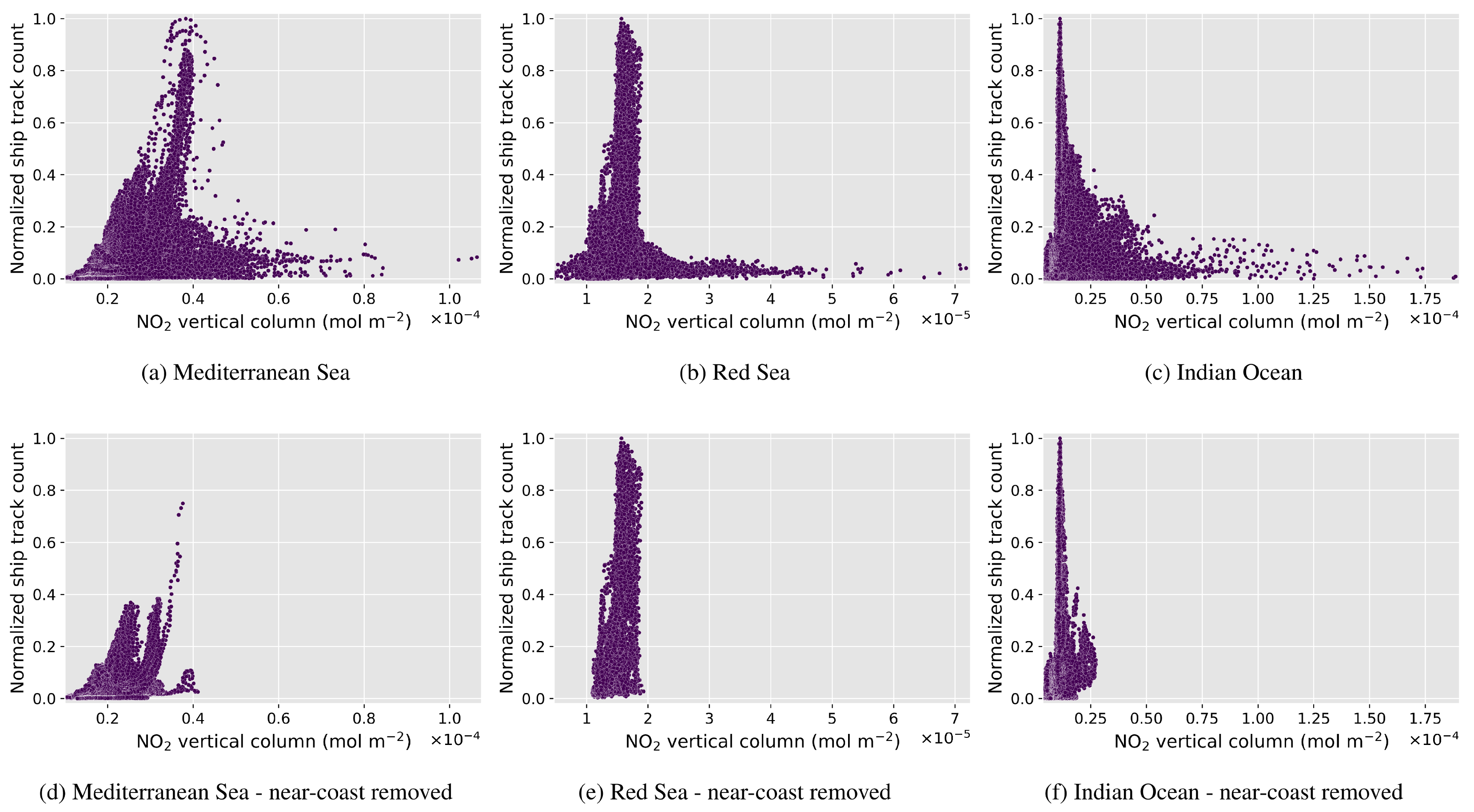
Figure A4.
Scatterplot of NO2 tropospheric VCD before and after near-coast removal. Since our interest is in shipping emissions, we removed the NO2 tropospheric VCD data that may have originated from irrelevant inland anthropogenic sources near the coast. The scatterplots on the left show the NO2 tropospheric VCD plotted against the ship track counts for the Mediterranean Sea, the Red Sea, and the Indian Ocean before near-coast removal (a–c), while those on the right show the same scatterplots after near-coast removal (d–f). Note that our technique effectively removes inland and near-coast NO2 tropospheric VCD, as evidenced by the removal of many observations with high NO2 tropospheric VCD but almost no ship tracks on the right-hand tails of the plots.

Figure A5.
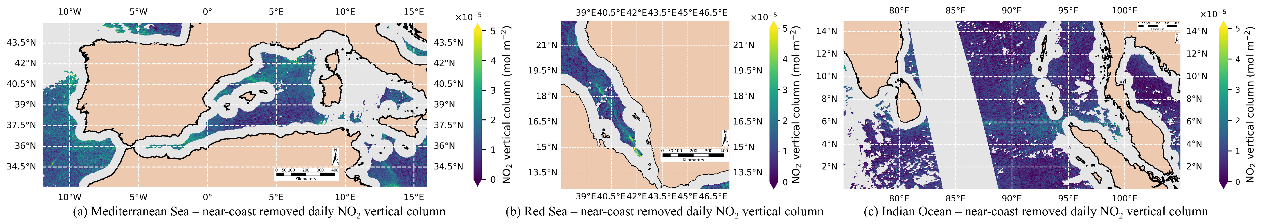
Visualization of the NO2 tropospheric VCD near-coast removal on a single day TROPOMI image. To ensure the accuracy of our analysis, we removed the NO2 column that may have originated from irrelevant inland anthropogenic emission sources. (a–c) TROPOMI-retrieved daily NO2 tropospheric VCD on 11 May 2021, for (a) the Mediterranean Sea, (b) the Red Sea, and (c) the Indian Ocean, with near-coast regions masked.
Figure A5.
Visualization of the NO2 tropospheric VCD near-coast removal on a single day TROPOMI image. To ensure the accuracy of our analysis, we removed the NO2 column that may have originated from irrelevant inland anthropogenic emission sources. (a–c) TROPOMI-retrieved daily NO2 tropospheric VCD on 11 May 2021, for (a) the Mediterranean Sea, (b) the Red Sea, and (c) the Indian Ocean, with near-coast regions masked.

Figure A6.
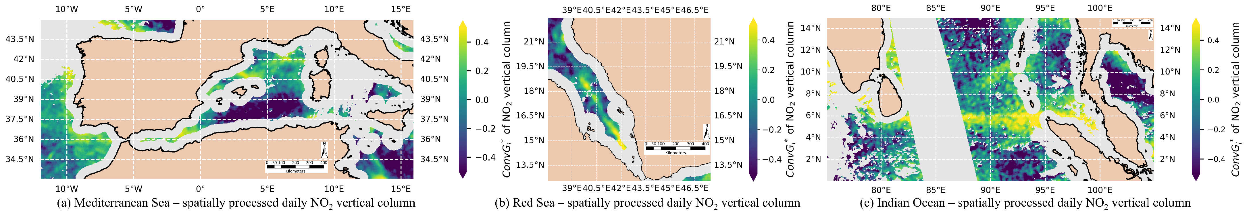
Visualization of the NO2 spatial autocorrelation processing on a single day TROPOMI image. (a–c) Spatial-standard score of the NO2 tropospheric VCD retrieved by TROPOMI on 11 May 2021 for (a) the Mediterranean Sea, (b) the Red Sea, and (c) the Indian Ocean. To account for the spatial autocorrelation present in the georeferenced TROPOMI data, we transform the NO2 column into the statistic, which represents a spatial-standardized and convolved Getis-Ord quantification.
Figure A6.
Visualization of the NO2 spatial autocorrelation processing on a single day TROPOMI image. (a–c) Spatial-standard score of the NO2 tropospheric VCD retrieved by TROPOMI on 11 May 2021 for (a) the Mediterranean Sea, (b) the Red Sea, and (c) the Indian Ocean. To account for the spatial autocorrelation present in the georeferenced TROPOMI data, we transform the NO2 column into the statistic, which represents a spatial-standardized and convolved Getis-Ord quantification.

Figure A7.
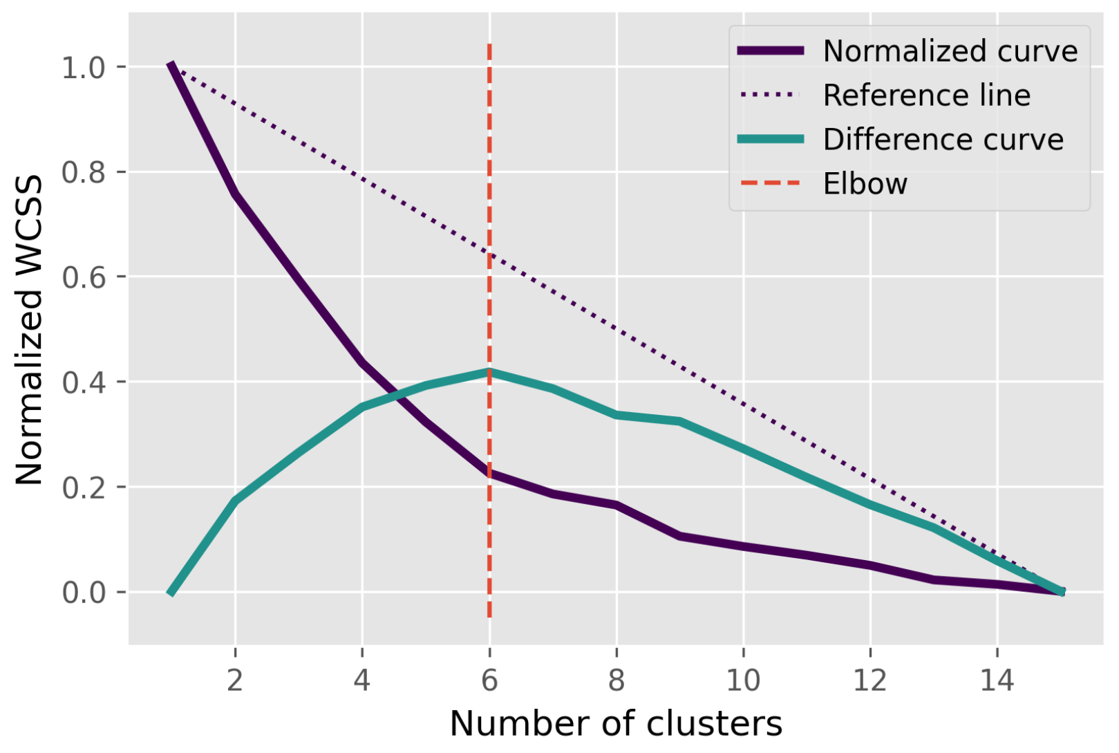
Illustration of the elbow method for determining the optimal number of clusters (k) in k-means clustering. The plot displays an example retrieved from the Indian Ocean NO2 column density. The normalized curve represents the normalized within-cluster sum of squares (WCSS) plotted per k clusters. The difference curve shows the magnitude of the difference between the normalized curve and its linear reference line. Clustering is performed on a spatio-temporally resolved scalar NO2 column density, with the number of clusters ranging from one to fifteen. The elbow point on the plot represents the optimal number of clusters for the given dataset.
Figure A7.
Illustration of the elbow method for determining the optimal number of clusters (k) in k-means clustering. The plot displays an example retrieved from the Indian Ocean NO2 column density. The normalized curve represents the normalized within-cluster sum of squares (WCSS) plotted per k clusters. The difference curve shows the magnitude of the difference between the normalized curve and its linear reference line. Clustering is performed on a spatio-temporally resolved scalar NO2 column density, with the number of clusters ranging from one to fifteen. The elbow point on the plot represents the optimal number of clusters for the given dataset.

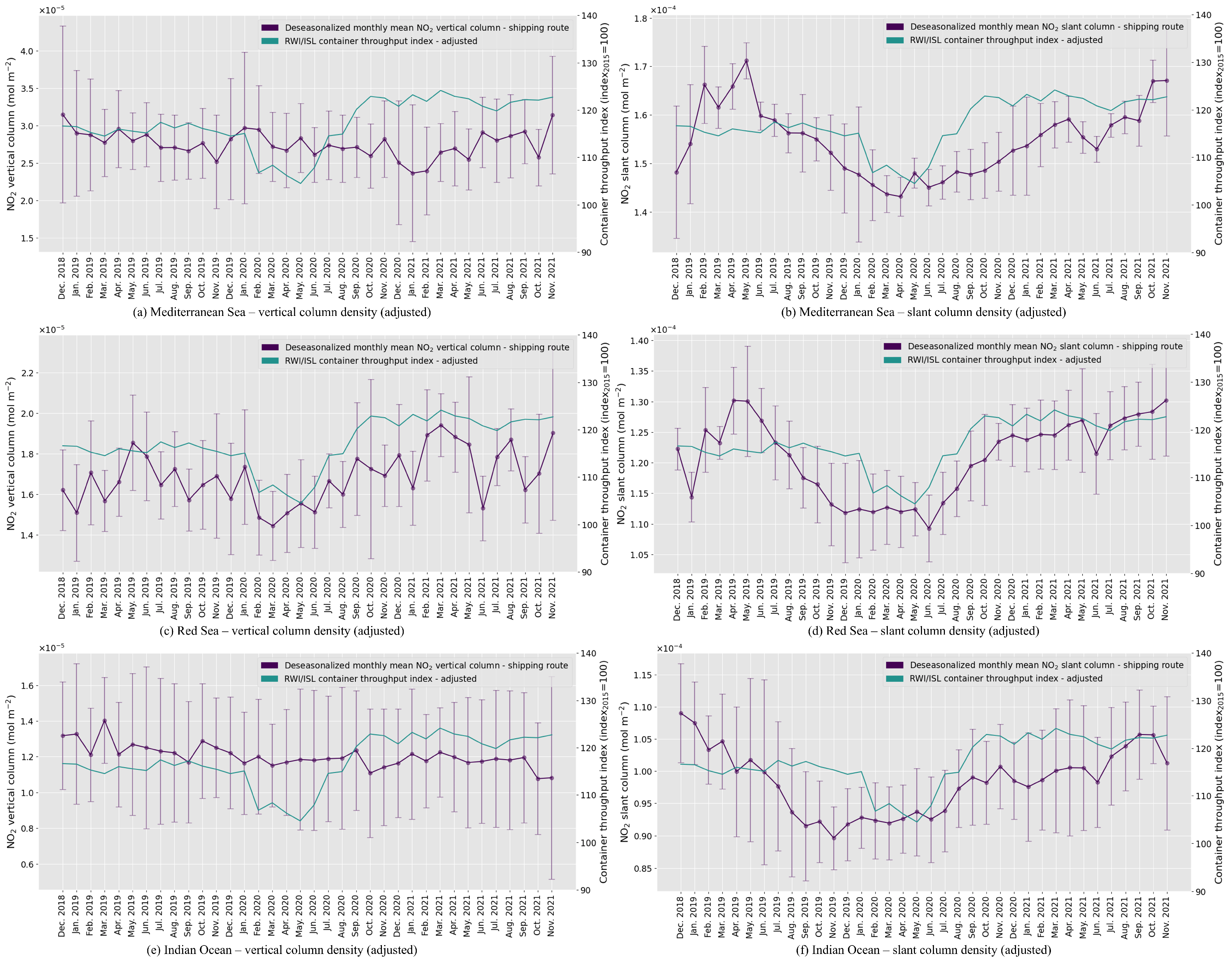
Figure A8.
Line plots showing the deseasonalized monthly averaged NO2 tropospheric VCD and slant column density (SCD) compared to the global container throughput adjusted index. (a,c,e) Deseasonalized monthly mean NO2 tropospheric VCD plotted together with the RWI/ISL Container Throughput Adjusted Index. (b,d,f) Deseasonalized monthly mean NO2 SCD plotted together with the same RWI/ISL Container Throughput Adjusted Index. The temporal trend analysis of the NO2 tropospheric VCD and SCD indicates that the NO2 SCD better reflects the fluctuation of the global container throughput index.

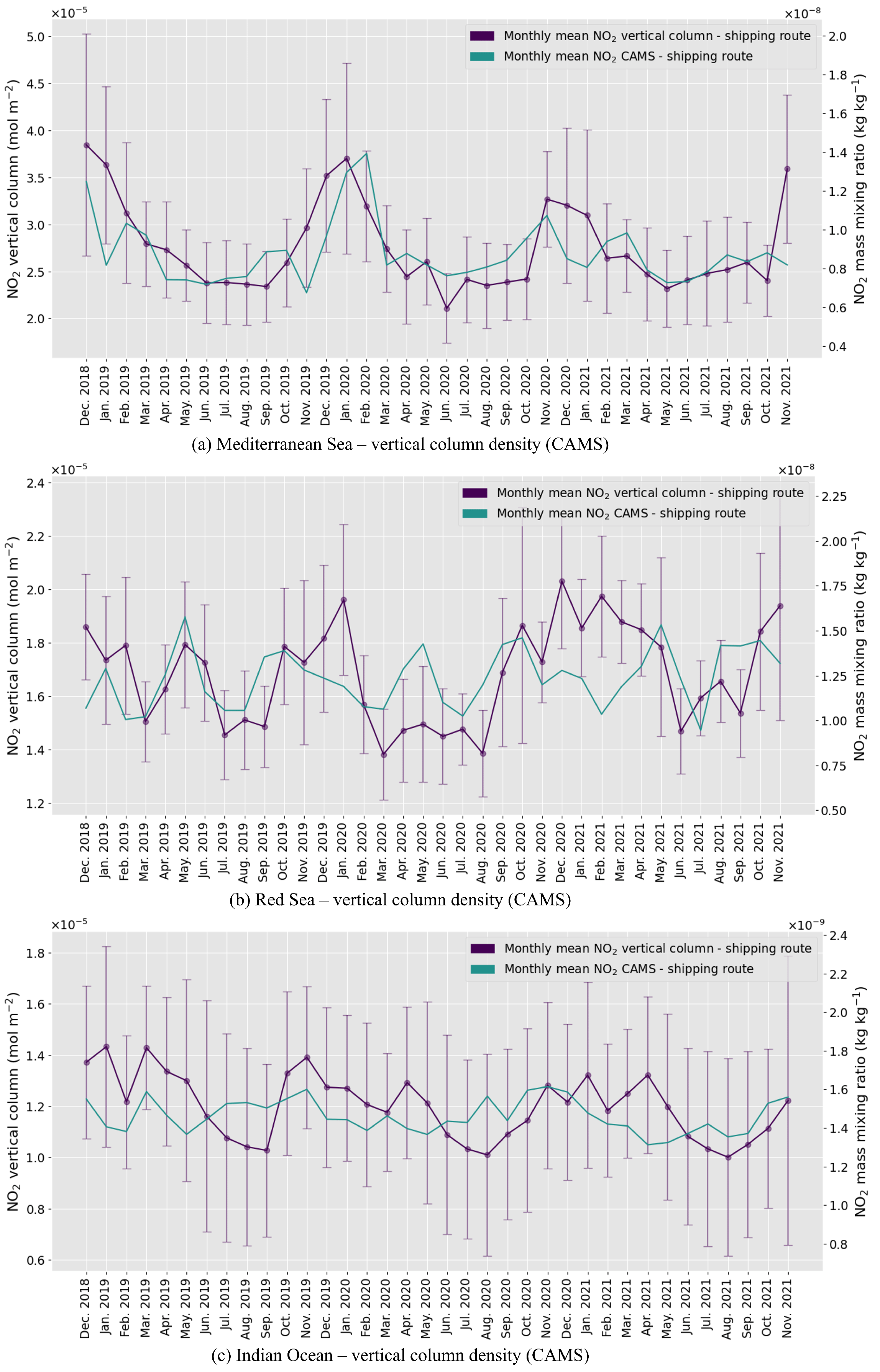
Figure A9.
Line plots showing the monthly mean NO2 tropospheric VCD and NO2 mixing ratio of shipping route, of (a) the Mediterranean Sea, (b) the Red Sea, and (c) the Indian Ocean. Monthly mean NO2 tropospheric VCD plotted together with the Copernicus Atmosphere Monitoring Service (CAMS) global reanalysis ECMWF Atmospheric Composition 4 (EAC4) data. The temporal trend analysis of the NO2 tropospheric VCD and NO2 CAMS indicates that the NO2 tropospheric VCD reflects the true global NO2 emission inventory represented by CAMS data.


Table A1.
Mean () and standard deviation () of the NO2 tropospheric VCD within clusters. The comparison is made between clusters generated without spatial preprocessing (Original) and clusters generated with proposed spatial preprocessing () for each test region. Each value corresponds to the NO2 tropospheric VCD, measured in units of 1 × 10⁻⁵ mol m−2. The number of clusters is determined using the elbow method, resulting in five clusters for the Mediterranean Sea (Medit. Sea), four clusters for the Red Sea, and six clusters for the Indian Ocean. Note that the cluster labels are sorted in ascending order of .
| Region | Type | Cluster 1 | Cluster 2 | Cluster 3 | Cluster 4 | Cluster 5 | Cluster 6 | ||||||
|---|---|---|---|---|---|---|---|---|---|---|---|---|---|
| Medit. | Original | 1.382 | 0.832 | 1.843 | 1.047 | 2.344 | 1.363 | 3.013 | 1.840 | 4.176 | 3.341 | - | - |
| Sea | 1.212 | 0.763 | 1.419 | 0.880 | 1.742 | 1.014 | 2.113 | 1.244 | 2.701 | 1.592 | - | - | |
| Red Sea | Original | 1.190 | 0.575 | 1.476 | 0.722 | 1.924 | 1.300 | 3.291 | 2.933 | - | - | - | - |
| 1.201 | 0.590 | 1.343 | 0.661 | 1.485 | 0.758 | 1.681 | 0.920 | - | - | - | - | ||
| Indian | Original | 0.561 | 0.513 | 0.870 | 0.570 | 1.220 | 0.739 | 1.954 | 1.241 | 3.797 | 3.036 | 9.504 | 8.190 |
| Ocean | 0.461 | 0.480 | 0.546 | 0.502 | 0.636 | 0.528 | 0.803 | 0.536 | 0.947 | 0.591 | 1.220 | 0.749 | |
Table A2.
Average NO2 tropospheric VCD and SCD per region, per year, and per cluster. Test regions span busy shipping routes, namely the Mediterranean Sea (Medit. Sea), the Red Sea, and the Indian Ocean. Test years span from the year 2019 to the year 2021. Clusters are distinguished as either shipping route (the cluster with the highest ship track counts) or background (the cluster with the lowest ship track counts). Each table entry represents the mean column density value within a cluster plus or minus one standard deviation, preprocessed with the method.
| Region | Average NO2 VCD—2019 | Average NO2 VCD—2020 | Average NO2 VCD—2021 | |||
|---|---|---|---|---|---|---|
| Shipping Route | Background | Shipping Route | Background | Shipping Route | Background | |
| Medit. Sea | 2.741 ± 1.627 | 1.208 ± 0.779 | 2.695 ± 1.552 | 1.235 ± 0.743 | 2.580 ± 1.461 | 1.166 ± 0.735 |
| Red Sea | 1.661 ± 0.948 | 1.160 ± 0.571 | 1.627 ± 0.910 | 1.168 ± 0.609 | 1.750 ± 0.898 | 1.273 ± 0.584 |
| Indian Ocean | 1.277 ± 0.714 | 0.490 ± 0.466 | 1.183 ± 0.748 | 0.442 ± 0.493 | 1.182 ± 0.789 | 0.453 ± 0.484 |
| Average NO2 SCD—2019 | Average NO2 SCD—2020 | Average NO2 SCD—2021 | ||||
| Shipping Route | Background | Shipping Route | Background | Shipping Route | Background | |
| Medit. Sea | 15.942 ± 2.552 | 14.515 ± 2.426 | 14.806 ± 2.297 | 13.677 ± 2.097 | 15.974 ± 2.374 | 14.842 ± 2.208 |
| Red Sea | 12.140 ± 2.194 | 11.500 ± 1.969 | 11.606 ± 1.815 | 11.017 ± 1.663 | 12.652 ± 1.942 | 12.118 ± 1.839 |
| Indian Ocean | 9.826 ± 1.731 | 8.225 ± 1.259 | 9.425 ± 1.610 | 8.187 ± 1.398 | 10.113 ± 1.751 | 8.727 ± 1.675 |
Table A3.
Relative change of NO2 tropospheric VCD and SCD per region and per cluster, calculated as a ratio between years. Test regions span busy shipping routes, namely the Mediterranean Sea (Medit. Sea), the Red Sea, and the Indian Ocean. Ratios between years span from the change over 2019–2020, over 2020–2021, and over 2019–2021. In each subcolumn heading, the notation of year ratio (e.g., year A/year B) stands for the average NO2 column density of year A divided by the average NO2 column density of year B. For each table entry, red font indicates an increase in the ratio (mean value larger than 1), while blue font indicates a decrease in the ratio (mean value smaller than 1). Clusters are distinguished as either shipping route (the cluster with the highest ship track counts) or background (the cluster with the lowest ship track counts). Each table entry represents the mean column density value within a cluster plus or minus one standard deviation, preprocessed with the method.
| Region | NO2 VCD Ratio—2020/2019 | NO2 VCD Ratio—2021/2020 | NO2 VCD Ratio—2021/2019 | |||
|---|---|---|---|---|---|---|
| Shipping Route | Background | Shipping Route | Background | Shipping Route | Background | |
| Medit. Sea | 0.985 ± 0.047 | 1.029 ± 0.065 | 0.954 ± 0.061 | 0.946 ± 0.047 | 0.939 ± 0.062 | 0.972 ± 0.070 |
| Red Sea | 0.980 ± 0.038 | 1.008 ± 0.039 | 1.077 ± 0.050 | 1.091 ± 0.059 | 1.055 ± 0.050 | 1.099 ± 0.048 |
| Indian Ocean | 0.930 ± 0.071 | 0.908 ± 0.098 | 0.999 ± 0.081 | 1.023 ± 0.119 | 0.925 ± 0.069 | 0.931 ± 0.102 |
| NO2 SCD Ratio—2020/2019 | NO2 SCD Ratio—2021/2020 | NO2 SCD Ratio—2021/2019 | ||||
| Shipping Route | Background | Shipping Route | Background | Shipping Route | Background | |
| Medit. Sea | 0.928 ± 0.012 | 0.941 ± 0.011 | 1.079 ± 0.012 | 1.084 ± 0.015 | 1.002 ± 0.015 | 1.021 ± 0.020 |
| Red Sea | 0.956 ± 0.008 | 0.957 ± 0.007 | 1.090 ± 0.010 | 1.099 ± 0.008 | 1.041 ± 0.009 | 1.052 ± 0.008 |
| Indian Ocean | 0.963 ± 0.025 | 0.996 ± 0.013 | 1.071 ± 0.025 | 1.066 ± 0.016 | 1.031 ± 0.016 | 1.061 ± 0.015 |
References
- Atkinson, R. Atmospheric chemistry of VOCs and NOx. Atmos. Environ. 2000, 34, 2063–2101. [Google Scholar] [CrossRef]
- Kampa, M.; Castanas, E. Human health effects of air pollution. Environ. Pollut. 2008, 151, 362–367. [Google Scholar] [CrossRef] [PubMed]
- United States Environmental Protection Agency. Nitrogen Dioxide (NO2) Pollution. Available online: https://www.epa.gov/no2-pollution (accessed on 4 July 2023).
- Chauhan, A.J.; Krishna, M.T.; Frew, A.J.; Holgate, S.T. Exposure to nitrogen dioxide (NO2) and respiratory disease risk. Rev. Environ. Health 1998, 13, 73–90. [Google Scholar] [PubMed]
- Pöschl, U.; Shiraiwa, M. Multiphase Chemistry at the Atmosphere–Biosphere Interface Influencing Climate and Public Health in the Anthropocene. Chem. Rev. 2015, 115, 4440–4475. [Google Scholar] [CrossRef] [PubMed]
- Corbett, J.J.; Fischbeck, P. Emissions from Ships. Science 1997, 278, 823–824. [Google Scholar] [CrossRef]
- Eyring, V.; Köhler, H.; van Aardenne, J.; Lauer, A. Emissions from international shipping: 1. The last 50 years. J. Geophys. Res. Atmos. 2005, 110, 1–12. [Google Scholar] [CrossRef]
- Corbett, J.J.; Winebrake, J.J.; Green, E.H.; Kasibhatla, P.; Eyring, V.; Lauer, A. Mortality from ship emissions: A global assessment. Environ. Sci. Technol. 2007, 41, 8512–8518. [Google Scholar] [CrossRef]
- International Maritime Organization. International Maritime Organization: Feb 2019 Supplement: MARPOL Annex VI & NTC 2008 (IC664E). 2019. Available online: https://wwwcdn.imo.org/localresources/en/publications/Documents/Supplements/English/QQC664E_022019.pdf (accessed on 21 June 2023).
- British Broadcasting Corporation. Shipping Industry Faces Calls to Clean Up Emissions. 2018. Available online: https://www.bbc.com/news/business-43696900 (accessed on 21 June 2023).
- Gerretsen, I. Shipping Is One of the Dirtiest Industries. Now It’s Trying to Clean Up Its Act. 2019. Available online: https://edition.cnn.com/2019/10/03/business/global-shipping-climate-crisis-intl/index.html (accessed on 21 June 2023).
- Palmer, C. Cruise Industry Faces Choppy Seas as It Tries to Clean Up Its Act On Climate. 2022. Available online: https://www.reuters.com/business/sustainable-business/cruise-industry-faces-choppy-seas-it-tries-clean-up-its-act-climate-2022-07-27/ (accessed on 21 June 2023).
- Veefkind, J.P.; Aben, I.; McMullan, K.; Förster, H.; de Vries, J.; Otter, G.; Claas, J.; Eskes, H.J.; de Haan, J.F.; Kleipool, Q.; et al. TROPOMI on the ESA Sentinel-5 Precursor: A GMES mission for global observations of the atmospheric composition for climate, air quality and ozone layer applications. Remote. Sens. Environ. 2012, 120, 70–83. [Google Scholar] [CrossRef]
- Georgoulias, A.K.; Boersma, K.F.; van Vliet, J.; Zhang, X.; van der A, R.; Zanis, P.; de Laat, J. Detection of NO2 pollution plumes from individual ships with the TROPOMI/S5P satellite sensor. Environ. Res. Lett. 2020, 15, 124037. [Google Scholar] [CrossRef]
- Okamura, B. Proposed IMO Regulations for the Prevention of Air Pollution from Ships. J. Marit. Law Commer. 1995, 26, 183–195. [Google Scholar]
- Halpern, B.; Frazier, M.; Potapenko, J.; Casey, K.; Koenig, K.; Longo, C.; Lowndes, J.S.; Rockwood, C.; Selig, E.; Selkoe, K.; et al. Spatial and temporal changes in cumulative human impacts on the world’s ocean. Nat. Commun. 2015, 6, 7615. [Google Scholar] [CrossRef] [Green Version]
- Institute of Shipping Economics and Logistics. RWI/ISL Container Throughput Input Index: Revival of Global Trade. 2023. Available online: https://www.isl.org/en/containerindex (accessed on 21 June 2023).
- Berg, N.; Mellqvist, J.; Jalkanen, J.P.; Balzani, J. Ship emissions of SO2 and NO2: DOAS measurements from airborne platforms. Atmos. Meas. Tech. 2012, 5, 1085–1098. [Google Scholar] [CrossRef] [Green Version]
- Alföldy, B.; Lööv, J.B.; Lagler, F.; Mellqvist, J.; Berg, N.; Beecken, J.; Weststrate, H.; Duyzer, J.; Bencs, L.; Horemans, B.; et al. Measurements of air pollution emission factors for marine transportation in SECA. Atmos. Meas. Tech. 2013, 6, 1777–1791. [Google Scholar] [CrossRef] [Green Version]
- Pirjola, L.; Pajunoja, A.; Walden, J.; Jalkanen, J.P.; Rönkkö, T.; Kousa, A.; Koskentalo, T. Mobile measurements of ship emissions in two harbour areas in Finland. Atmos. Meas. Tech. 2014, 7, 149–161. [Google Scholar] [CrossRef] [Green Version]
- Lööv, J.; Alföldy, B.; Gast, L.; Hjorth, J.; Lagler, F.; Mellqvist, J.; Beecken, J.; Berg, N.; Duyzer, J.; Westrate, H.; et al. Field test of available methods to measure remotely SOx and NOx emissions from ships. Atmos. Meas. Tech. Discuss. 2013, 7, 2597–2613. [Google Scholar] [CrossRef] [Green Version]
- Richter, A.; Eyring, V.; Burrows, J.P.; Bovensmann, H.; Lauer, A.; Sierk, B.; Crutzen, P.J. Satellite measurements of NO2 from international shipping emissions. Geophys. Res. Lett. 2004, 31, L23110. [Google Scholar] [CrossRef]
- Boersma, K.F.; Vinken, G.C.M.; Tournadre, J. Ships going slow in reducing their NOx emissions: Changes in 2005–2012 ship exhaust inferred from satellite measurements over Europe. Environ. Res. Lett. 2015, 10, 074007. [Google Scholar] [CrossRef] [Green Version]
- Riess, T.C.V.W.; Boersma, K.F.; van Vliet, J.; Peters, W.; Sneep, M.; Eskes, H.; van Geffen, J. Improved monitoring of shipping NO2 with TROPOMI: Decreasing NOx emissions in European seas during the COVID-19 pandemic. Atmos. Meas. Tech. 2022, 15, 1415–1438. [Google Scholar] [CrossRef]
- Tobler, W.R. A Computer Movie Simulating Urban Growth in the Detroit Region. Econ. Geogr. 1970, 46, 234–240. [Google Scholar] [CrossRef]
- Haining, R. Spatial Autocorrelation. In International Encyclopedia of the Social & Behavioral Sciences, 2nd ed.; Wright, J.D., Ed.; Elsevier: Oxford, UK, 2015; pp. 105–110. [Google Scholar] [CrossRef]
- Heckel, A.; Kim, S.W.; Frost, G.J.; Richter, A.; Trainer, M.; Burrows, J.P. Influence of low spatial resolution a priori data on tropospheric NO2 satellite retrievals. Atmos. Meas. Tech. 2011, 4, 1805–1820. [Google Scholar] [CrossRef] [Green Version]
- Sun, K.; Zhu, L.; Cady-Pereira, K.; Chan Miller, C.; Chance, K.; Clarisse, L.; Coheur, P.F.; González Abad, G.; Huang, G.; Liu, X.; et al. A physics-based approach to oversample multi-satellite, multispecies observations to a common grid. Atmos. Meas. Tech. 2018, 11, 6679–6701. [Google Scholar] [CrossRef] [Green Version]
- Zhu, L.; Jacob, D.J.; Keutsch, F.N.; Mickley, L.J.; Scheffe, R.; Strum, M.; González Abad, G.; Chance, K.; Yang, K.; Rappenglück, B.; et al. Formaldehyde (HCHO) As a Hazardous Air Pollutant: Mapping Surface Air Concentrations from Satellite and Inferring Cancer Risks in the United States. Environ. Sci. Technol. 2017, 51, 5650–5657. [Google Scholar] [CrossRef] [PubMed]
- Dix, B.; de Bruin, J.; Roosenbrand, E.; Vlemmix, T.; Francoeur, C.; Gorchov-Negron, A.; McDonald, B.; Zhizhin, M.; Elvidge, C.; Veefkind, P.; et al. Nitrogen Oxide Emissions from U.S. Oil and Gas Production: Recent Trends and Source Attribution. Geophys. Res. Lett. 2019, 41, 1–9. [Google Scholar] [CrossRef]
- Goldberg, D.L.; Lu, Z.; Streets, D.G.; de Foy, B.; Griffin, D.; McLinden, C.A.; Lamsal, L.N.; Krotkov, N.A.; Eskes, H. Enhanced Capabilities of TROPOMI NO2: Estimating NOx from North American Cities and Power Plants. Environ. Sci. Technol. 2019, 53, 12594–12601. [Google Scholar] [CrossRef]
- Goldberg, D.L.; Anenberg, S.; Mohegh, A.; Lu, Z.; Streets, D.G. TROPOMI NO2 in the United States: A detailed look at the annual averages, weekly cycles, effects of temperature, and correlation with surface NO2 concentrations. Earth’s Future 2021, 9, e2020EF001665. [Google Scholar] [CrossRef]
- Cooper, M.J.; Martin, R.V.; Hammer, M.S.; Levelt, P.F.; Veefkind, P.; Lamsal, L.N.; Krotkov, N.A.; Brook, J.R.; McLinden, C.A. Global fine-scale changes in ambient NO2 during COVID-19 lockdowns. Nature 2022, 601, 380–387. [Google Scholar] [CrossRef]
- Souri, A.H.; Choi, Y.; Pan, S.; Curci, G.; Nowlan, C.R.; Janz, S.J.; Kowalewski, M.G.; Liu, J.; Herman, J.R.; Weinheimer, A.J. First Top-Down Estimates of Anthropogenic NOx Emissions Using High-Resolution Airborne Remote Sensing Observations. J. Geophys. Res. Atmos. 2018, 123, 3269–3284. [Google Scholar] [CrossRef]
- Kurchaba, S.; van Vliet, J.; Meulman, J.J.; Verbeek, F.J.; Veenman, C.J. Improving Evaluation of NO2 Emission from Ships Using Spatial Association on TROPOMI Satellite Data. In Proceedings of the 29th International Conference on Advances in Geographic Information Systems, 2021—SIGSPATIAL ’21, New York, NY, USA, 2–5 November 2021; pp. 454–457. [Google Scholar] [CrossRef]
- Kurchaba, S.; van Vliet, J.; Verbeek, F.J.; Meulman, J.J.; Veenman, C.J. Supervised Segmentation of NO2 Plumes from Individual Ships Using TROPOMI Satellite Data. Remote. Sens. 2022, 14, 5809. [Google Scholar] [CrossRef]
- Kubat, M.; Holte, R.; Matwin, S. Machine Learning for the Detection of Oil Spills in Satellite Radar Images. Mach. Learn. 1998, 30, 195–215. [Google Scholar] [CrossRef] [Green Version]
- Kuhn, M.; Johnson, K. Applied Predictive Modeling; Springer: New York, NY, USA, 2013. [Google Scholar] [CrossRef]
- United States Environmental Protection Agency. Nitrogen Oxides (NOx): Why and How They Are Controlled; EPA-456/F-99-006R. 1999. Available online: https://www3.epa.gov/ttn/catc/cica/files/fnoxdoc.pdf (accessed on 21 June 2023).
- Reşitoğlu, I.A.; Altinişik, K.; Keskin, A. The pollutant emissions from diesel-engine vehicles and exhaust aftertreatment systems. Clean Technol. Environ. Policy 2015, 17, 15–27. [Google Scholar] [CrossRef] [Green Version]
- Burrows, J.P.; Weber, M.; Buchwitz, M.; Rozanov, V.; Ladstätter-Weißenmayer, A.; Richter, A.; DeBeek, R.; Hoogen, R.; Bramstedt, K.; Eichmann, K.; et al. The Global Ozone Monitoring Experiment (GOME): Mission Concept and First Scientific Results. J. Atmos. Sci. 1999, 56, 151–175. [Google Scholar] [CrossRef]
- Levelt, P.F.; van den Oord, G.H.J.; Dobber, M.R.; Malkki, A.; Visser, H.; de Vries, J.; Stammes, P.; Lundell, J.O.V.; Saari, H. The ozone monitoring instrument. IEEE Trans. Geosci. Remote. Sens. 2006, 44, 1093–1101. [Google Scholar] [CrossRef]
- van Geffen, J.H.G.M.; Eskes, H.J.; Boersma, K.F.; Veefkind, J.P. TROPOMI ATBD of the Total and Tropospheric NO2 Data Products; Technical Report; Royal Netherlands Meteorological Institute: De Bilt, The Netherlands, 2022. [Google Scholar]
- Platt, U.; Perner, D. Measurements of Atmospheric Trace Gases by Long Path Differential UV/Visible Absorption Spectroscopy; Springer Series in Optical Sciences 39; Springer: Berlin/Heidelberg, Germany, 1983; pp. 95–110. [Google Scholar]
- Stutz, J.; Platt, U. Numerical analysis and estimation of the statistical error of differential optical absorption spectroscopy measurements with least-squares methods. Appl. Opt. 1996, 35, 6041–6053. [Google Scholar] [CrossRef] [Green Version]
- Platt, U.; Stutz, J. Differential Optical Absorption Spectroscopy: Principles and Applications; Physics of Earth and Space Environments; Springer: Berlin/Heidelberg, Germany, 2008; Volume 127. [Google Scholar] [CrossRef] [Green Version]
- Rew, R.; Davis, G. NetCDF: An interface for scientific data access. IEEE Comput. Graph. Appl. 1990, 10, 76–82. [Google Scholar] [CrossRef]
- Eskes, H.; van Geffen, J.; Boersma, F.; Eichmann, K.U.; Apituley, A.; Pedergnana, M.; Sneep, M.; Veefkind, J.P.; Loyola, D. Sentinel-5 Precursor/TROPOMI Level 2 Product User Manual Nitrogendioxide. 2022. Available online: https://sentinel.esa.int/documents/247904/2474726/Sentinel-5P-Level-2-Product-User-Manual-Nitrogen-Dioxide.pdf (accessed on 21 June 2023).
- Natural Earth Data. Free Vector and Raster Map Data at 1:10m, 1:50m, and 1:110m Scales [data set]. 2022. Available online: https://www.naturalearthdata.com/ (accessed on 21 June 2023).
- Haralick, R.M.; Sternberg, S.R.; Zhuang, X. Image Analysis Using Mathematical Morphology. IEEE Trans. Pattern Anal. Mach. Intell. 1987, PAMI-9, 532–550. [Google Scholar] [CrossRef]
- LeSage, J.P. An Introduction to Spatial Econometrics. Rev. Econ. Ind. 2008, 123, 19–44. [Google Scholar] [CrossRef] [Green Version]
- LeSage, J.P.; Pace, R.K. Introduction to Spatial Econometrics; Statistics: A Series of Textbooks and Monographs; Chapman & Hall/CRC: Boca Raton, FL, USA, 2009. [Google Scholar]
- Thorpe, A.K.; Frankenberg, C.; Thompson, D.R.; Duren, R.M.; Aubrey, A.D.; Bue, B.D.; Green, R.O.; Gerilowski, K.; Krings, T.; Borchardt, J.; et al. Airborne DOAS retrievals of methane, carbon dioxide, and water vapor concentrations at high spatial resolution: Application to AVIRIS-NG. Atmos. Meas. Tech. 2017, 10, 3833–3850. [Google Scholar] [CrossRef] [Green Version]
- Getis, A.; Ord, J.K. The Analysis of Spatial Association by Use of Distance Statistics. Geogr. Anal. 1992, 24, 189–206. [Google Scholar] [CrossRef]
- Anselin, L. Local Indicators of Spatial Association—LISA. Geogr. Anal. 1995, 27, 93–115. [Google Scholar] [CrossRef]
- Nowlan, C.R.; Liu, X.; Janz, S.J.; Kowalewski, M.G.; Chance, K.; Follette-Cook, M.B.; Fried, A.; González Abad, G.; Herman, J.R.; Judd, L.M.; et al. Nitrogen dioxide and formaldehyde measurements from the GEOstationary Coastal and Air Pollution Events (GEO-CAPE) Airborne Simulator over Houston, Texas. Atmos. Meas. Tech. 2018, 11, 5941–5964. [Google Scholar] [CrossRef] [Green Version]
- Judd, L.M.; Al-Saadi, J.A.; Szykman, J.J.; Valin, L.C.; Janz, S.J.; Kowalewski, M.G.; Eskes, H.J.; Veefkind, J.P.; Cede, A.; Mueller, M.; et al. Evaluating Sentinel-5P TROPOMI tropospheric NO2 column densities with airborne and Pandora spectrometers near New York City and Long Island Sound. Atmos. Meas. Tech. 2020, 13, 6113–6140. [Google Scholar] [CrossRef] [PubMed]
- Motulsky, H.J.; Brown, R.E. Detecting outliers when fitting data with nonlinear regression—A new method based on robust nonlinear regression and the false discovery rate. BMC Bioinform. 2006, 7, 123. [Google Scholar] [CrossRef] [PubMed] [Green Version]
- Ord, J.K.; Getis, A. Local Spatial Autocorrelation Statistics: Distributional Issues and an Application. Geogr. Anal. 1995, 27, 286–306. [Google Scholar] [CrossRef]
- ArcGIS. How Generate Spatial Weights Matrix Works. Available online: https://pro.arcgis.com/en/pro-app/latest/tool-reference/spatial-statistics/how-generate-spatial-weights-matrix-spatial-statis.htm (accessed on 21 June 2023).
- Pace, R.K.; Barry, R. Sparse spatial autoregressions. Stat. Probab. Lett. 1997, 33, 291–297. [Google Scholar] [CrossRef]
- Shapiro, L.G.; Stockman, G.C. Computer Vision; Prentice Hall: Hoboken, NJ, USA, 2001. [Google Scholar]
- Roh, M.I. Determination of an economical shipping route considering the effects of sea state for lower fuel consumption. Int. J. Nav. Archit. Ocean. Eng. 2013, 5, 246–262. [Google Scholar] [CrossRef] [Green Version]
- Steinhaus, H. Sur la division des corps materiels en parties. Bull. Acad. Pol. Sci. 1956, 4, 801–804. [Google Scholar]
- Lloyd, S.P. Least squares quantization in PCM. Bell Telephone Laboratories Paper. Published in journal much later: Lloyd, S.P.: Least squares quantization in PCM. IEEE Trans. Inf. Theory 1982, 28, 129–137. [Google Scholar] [CrossRef] [Green Version]
- MacQueen, J.B. Some methods for classification and analysis of multivariate observations. In Proceedings of the Fifth Berkeley Symposium on Mathematical Statistics and Probability, Berkeley, CA, USA, 21 June–18 July 1965; University of California Press: Berkeley, CA, USA, 1967; Volume 1, pp. 281–297. [Google Scholar]
- Jain, A.; Murty, M.; Flynn, P. Data clustering: A review. ACM Comput. Surv. 1999, 31, 264–323. [Google Scholar] [CrossRef]
- Jarvis, R.; Patrick, E. Clustering Using a Similarity Measure Based on Shared Near Neighbors. IEEE Trans. Comput. 1973, C-22, 1025–1034. [Google Scholar] [CrossRef]
- Arthur, D.; Vassilvitskii, S. K-means++: The advantages of careful seeding. In Proceedings of the Eighteenth Annual ACM-SIAM Symposium on Discrete Algorithms, New Orleans, LO, USA, 7–9 January 2007; pp. 1027–1035. [Google Scholar]
- Thorndike, R.L. Who belongs in the family? Psychometrika 1953, 18, 267–276. [Google Scholar] [CrossRef]
- Hamilton, J.D. Measuring global economic activity. J. Appl. Econom. 2019, 36, 293–303. [Google Scholar] [CrossRef]
- Michail, N.A. World economic growth and seaborne trade volume: Quantifying the relationship. Transp. Res. Interdiscip. Perspect. 2020, 4, 100108. [Google Scholar] [CrossRef]
- United Nations Conference on Trade and Development. COVID-19 and Maritime Transport: Impact and Responses. Available online: https://unctad.org/webflyer/covid-19-and-maritime-transport-impact-and-responses (accessed on 21 June 2023).
- Verschuur, J.; Koks, E.E.; Hall, J.W. Global economic impacts of COVID-19 lockdown measures stand out in high-frequency shipping data. PLoS ONE 2021, 16, e0248818. [Google Scholar] [CrossRef]
- Koyuncu, K.; Tavacioğlu, L.; Gökmen, N.; Çelen Arican, U. Forecasting COVID-19 impact on RWI/ISL container throughput index by using SARIMA models. Marit. Policy Manag. 2021, 48, 1096–1108. [Google Scholar] [CrossRef]
- Persons, W.M. General Considerations and Assumptions. Rev. Econ. Stat. 1919, 1, 5–107. [Google Scholar] [CrossRef]
- Copernicus Atmosphere Monitoring Service. CAMS Global Reanalysis (EAC4). 2019. Available online: https://www.ecmwf.int/en/forecasts/dataset/cams-global-reanalysis (accessed on 21 June 2023).
- Eskes, H.J.; Boersma, K.F. Averaging kernels for DOAS total-column satellite retrievals. Atmos. Chem. Phys. 2003, 3, 1285–1291. [Google Scholar] [CrossRef] [Green Version]
- Richter, A.; Hilboll, A.; Burrows, J.P. Improving satellite retrievals of large tropospheric NO2 columns. In Proceedings of the Geophysical Research Abstracts, EGU General Assembly 2014, Vienna, Austria, 27 April–2 May 2014; Volume 16. [Google Scholar]
- Lorente, A.; Boersma, K.F.; Yu, H.; Dörner, S.; Hilboll, A.; Richter, A.; Liu, M.; Lamsal, L.N.; Barkley, M.; De Smedt, I.; et al. Structural uncertainty in air mass factor calculation for NO2 and HCHO satellite retrievals. Atmos. Meas. Tech. 2017, 10, 759–782. [Google Scholar] [CrossRef] [Green Version]
- Corbett, J.J.; Fischbeck, P.S.; Pandis, S.N. Global nitrogen and sulfur inventories for oceangoing ships. J. Geophys. Res. 1999, 104, 3457–3470. [Google Scholar] [CrossRef]
- Verhoelst, T.; Compernolle, S.; Pinardi, G.; Lambert, J.C.; Eskes, H.J.; Eichmann, K.U.; Fjæraa, A.M.; Granville, J.; Niemeijer, S.; Cede, A.; et al. Ground-based validation of the Copernicus Sentinel-5P TROPOMI NO2 measurements with the NDACC ZSL-DOAS, MAX-DOAS and Pandonia global networks. Atmos. Meas. Tech. 2021, 14, 481–510. [Google Scholar] [CrossRef]
Figure 1.
Visualization of International Maritime Organization (IMO) regulations on the emission of nitrogen oxides (NOx) from sea-faring ships. The NOx emission from ships depends on the engine’s rated speed and total weighted cycle emission limit, distinguished into three tiers based on the construction date of ships. Tier I is the NOx regulation imposed on ships constructed on/after 1 January 2000; Tier II is the NOx regulation imposed on ships constructed on/after 1 January 2011; and Tier III is the NOx regulation imposed on ships constructed on/after 1 January 2016.

Figure 2.
Schematic representation of identifying shipping emissions using remote sensing. The purple cylinder represents the database containing the original remote sensing measurements. The blue rectangle illustrates the systematic approach proposed in this paper. The green cylinder represents the auxiliary database used for validation. The yellow hexagon denotes the final output of the spatial or temporal patterns.

Figure 3.
Visualization of TROPOspheric Monitoring Instrument (TROPOMI) NO2 tropospheric vertical column density (VCD) data and ship track data [16]. Inland data are masked as empty in the original array, but filled with a desert sand color for visual separation. (a–c) Daily heatmaps of the NO2 tropospheric VCD retrieved by TROPOMI on 11 May 2021, for their respective regions. Gray areas indicate masked data due to low-quality assurance value or high cloud fraction. When oversampled, these daily events of high NO2 tropospheric VCD along the shipping route are not clearly visible, as shown in Figure A1. (d–f) Normalized ship track counts as an estimate of the shipping route for their respective regions.

Figure 4.
Visualization of clustered NO2 tropospheric VCD before and after near-coast pixel removal and spatio-temporal data preprocessing for their respective regions. (a–c) Clustering results using conventionally oversampled NO2 tropospheric VCD. (d–f) Clustering results using spatio-temporally preprocessed NO2 tropospheric VCD after removing near-coast pixels and applying the operation. The number of clusters per region is chosen using the elbow method [70] with five clusters for the Mediterranean Sea, four clusters for the Red Sea, and six clusters for the Indian Ocean.

Figure 5.
Boxplots of normalized ship track counts in each NO2 cluster. (a–c) Boxplots before near-coast removal and calculation on (a) the Mediterranean Sea, (b) the Red Sea, and (c) the Indian Ocean. (d,e) Boxplots after near-coast removal and calculation on (d) the Mediterranean Sea, (e) the Red Sea, and (f) the Indian Ocean. A red triangle in each boxplot indicates the mean value of the normalized ship track counts in the corresponding NO2 cluster. Fliers are not displayed to enhance the visualization of whiskers. The number of clusters per region is chosen by the elbow method [70] with five clusters for the Mediterranean Sea, four clusters for the Red Sea, and six clusters for the Indian Ocean. The higher the label of the NO2 cluster, the greater the average NO2 column density in that cluster, as illustrated in Table A1. Boxplot color in each panel corresponds to that of cluster labels in the corresponding panel of Figure 4. Note that spatially preprocessed cluster labels exhibit better representation of the ship track, as a higher NO2 concentration corresponds to a higher cluster label.

Figure 6.
Line plots showing the monthly averaged NO2 tropospheric VCD and NO2 tropospheric slant column density (SCD) compared to the global container throughput index. (a,c,e) Monthly mean NO2 tropospheric VCD plotted together with the Rheinisch-Westfälisches Institut für Wirtschaftsforschung and the Institute of Shipping Economics and Logistics (RWI/ISL) Container Throughput Index. (b,d,f) Monthly mean NO2 tropospheric SCD plotted together with the same RWI/ISL Container Throughput Index. The temporal trend analysis of the NO2 tropospheric VCD and tropospheric SCD indicates that the NO2 tropospheric SCD better reflects the fluctuation of the global container throughput index.

Table 1.
Spatio-temporal coverage of the six different TROPOMI NO2 datasets used.
| Dataset | Latitudinal Coverage | Longitudinal Coverage | Temporal Coverage |
|---|---|---|---|
| Mediterranean Sea—VCD | 33.015625N–44.984375N | 11.98438W–15.98438E | |
| Mediterranean Sea—SCD | (384 pixels) | (896 pixels) | |
| Red Sea—VCD | 12.515625N–22.484375N | 37.51563E–47.48438E | 5 Dec 2018–10 Nov 2021 |
| Red Sea—SCD | (320 pixels) | (320 pixels) | (1072 days) |
| Indian Ocean—VCD | 0.015625N–14.984375N | 75.01563E–104.98438E | |
| Indian Ocean—SCD | (480 pixels) | (960 pixels) |
Table 2.
Spatial correlation between the global container throughput index and three types of NO2 tropospheric VCD data: (1) original NO2 tropospheric VCD data; (2) clustered NO2 tropospheric VCD data without proposed spatial preprocessing; (3) clustered NO2 tropospheric VCD data using proposed spatial preprocessing. The highest spatial correlation value per test region is highlighted. The p-values of correlation coefficients are shown in parentheses.
| Test Region | Original NO2 Data | Clustered NO2 Data without | Clustered NO2 Data with |
|---|---|---|---|
| Mediterranean Sea | 0.4479 * (0.0000) | 0.4586 * (0.0000) | 0.5013 * (0.0000) |
| Red Sea | 0.1508 * (0.0000) | 0.2549 * (0.0000) | 0.6235 * (0.0000) |
| Indian Ocean | 0.2357 * (0.0000) | 0.3194 * (0.0000) | 0.3215 * (0.0000) |
p-values are in parentheses; * p < 0.01.
Table 3.
Temporal correlation between the global container throughput index and two types of NO2 column data: NO2 tropospheric VCD of shipping route and NO2 tropospheric SCD of shipping route. Each column density is divided into the original set and seasonally adjusted set. Deseasonalized column density is shown in Figure A8. The highest temporal correlation value per test region is highlighted. The p-values of correlation coefficients are shown in parentheses.
| Region | NO2 VCD of Shipping Route | NO2 SCD of Shipping Route | ||
|---|---|---|---|---|
| Original | Adjusted | Original | Adjusted | |
| Medit. Sea | −0.2523 (0.1376) | −0.1857 (0.2781) | 0.5567 * (0.0004) | 0.4582 * (0.0049) |
| Red Sea | 0.1992 (0.2442) | 0.6824 * (0.0000) | 0.6003 * (0.0001) | 0.7103 * (0.0000) |
| Indian Ocean | −0.2244 (0.1883) | −0.1915 (0.2632) | 0.5544 * (0.0005) | 0.5188 * (0.0012) |
p-values are in parentheses; * p < 0.01.
Disclaimer/Publisher’s Note: The statements, opinions and data contained in all publications are solely those of the individual author(s) and contributor(s) and not of MDPI and/or the editor(s). MDPI and/or the editor(s) disclaim responsibility for any injury to people or property resulting from any ideas, methods, instructions or products referred to in the content. |
© 2023 by the authors. Licensee MDPI, Basel, Switzerland. This article is an open access article distributed under the terms and conditions of the Creative Commons Attribution (CC BY) license (https://creativecommons.org/licenses/by/4.0/).
Share and Cite
MDPI and ACS Style
Kim, J.; Emmerich, M.T.M.; Voors, R.; Ording, B.; Lee, J.-S. A Systematic Approach to Identify Shipping Emissions Using Spatio-Temporally Resolved TROPOMI Data. Remote Sens. 2023, 15, 3453. https://doi.org/10.3390/rs15133453
AMA Style
Kim J, Emmerich MTM, Voors R, Ording B, Lee J-S. A Systematic Approach to Identify Shipping Emissions Using Spatio-Temporally Resolved TROPOMI Data. Remote Sensing. 2023; 15(13):3453. https://doi.org/10.3390/rs15133453
Chicago/Turabian StyleKim, Juhuhn, Michael T. M. Emmerich, Robert Voors, Barend Ording, and Jong-Seok Lee. 2023. "A Systematic Approach to Identify Shipping Emissions Using Spatio-Temporally Resolved TROPOMI Data" Remote Sensing 15, no. 13: 3453. https://doi.org/10.3390/rs15133453
Note that from the first issue of 2016, this journal uses article numbers instead of page numbers. See further details here.