1. Introduction
Atmospheric ozone O
3 is one of the most important minor gases in the atmosphere. Stratospheric ozone protects life on Earth from harmful UV-B solar radiation. The absorption of radiation by ozone determines the temperature profile of the stratosphere and influences its dynamics. Production and loss of ozone in the middle atmosphere in main features can be explained by oxygen chemistry [
1]. In fact, ozone loss is controlled not only by photodissociation and reaction between O
3 and atomic oxygen O. The catalytic reaction of ozone with radicals of odd hydrogen HO
x (H, OH, and HO
2), nitrogen NO
x (N, NO, and NO
2), and chlorine Cl
x (Cl and ClO) groups are very important as well [
1,
2]. In the mesosphere (altitudes
A = 50–90 km), ozone destruction in reactions with the HO
x radicals is usually dominant. Concentrations of the NO
x and HO
x components and rates of catalytic destruction of ozone by the species considerably increase under the ionization of the mesosphere in polar and subpolar latitudes due to energetic charged particles (electrons and protons) [
3,
4].
Solar eclipses are relatively short events, about 2 h at local ground-based observations. If the eclipse occurs at midday, both the solar zenith angle (SZA) and solar spectrum in the mesosphere change little during the eclipse. Thus, solar eclipses provide a unique possibility for experimentally studying the photochemistry of mesospheric ozone and testing photochemical models. The photochemical lifetime of ozone in the mesosphere is small, about 100 s [
1,
2], and ozone content follows the intensity of solar radiation with negligible delay. This case is much simpler for analysis than the diurnal ozone variations during sunrises and sunsets when significant changes in the optical depth of the atmosphere at SZA close to 90°, drastically changing the intensity and spectrum of solar radiation.
Up to now, only a few observations of mesospheric ozone during solar eclipses have been conducted using rockets [
5], in near-IR [
6], and at millimeter and submillimeter waves [
7,
8,
9]. The most interesting and detailed results were reported in [
9], where mesospheric ozone was observed during the solar eclipse of 15 January 2010 at frequencies of about 625 GHz from aboard the International Space Station. It was found in [
9] that changes in the ozone mixing ratio (OMR) profiles at altitudes of 58–70 km in dependence on the Sun’s obscuration during the eclipse were in good agreement with predictions of the comprehensive work on ozone chemistry in the mesosphere and lower thermosphere (MLT region, altitudes
A = 50–100 km) [
2]. Other observations [
5,
6,
7,
8] were not as complete and precise as [
9], and their data were not robustly analyzed. Atmospheric pressure and concentrations of ozone drop rapidly with increasing altitude. Thus, it is most convenient to use the OMR profile
CO3 (
A) expressed in ppm (parts per million, 10
−6) units instead of the ozone concentration [O
3] profiles expressed in cm
−3.
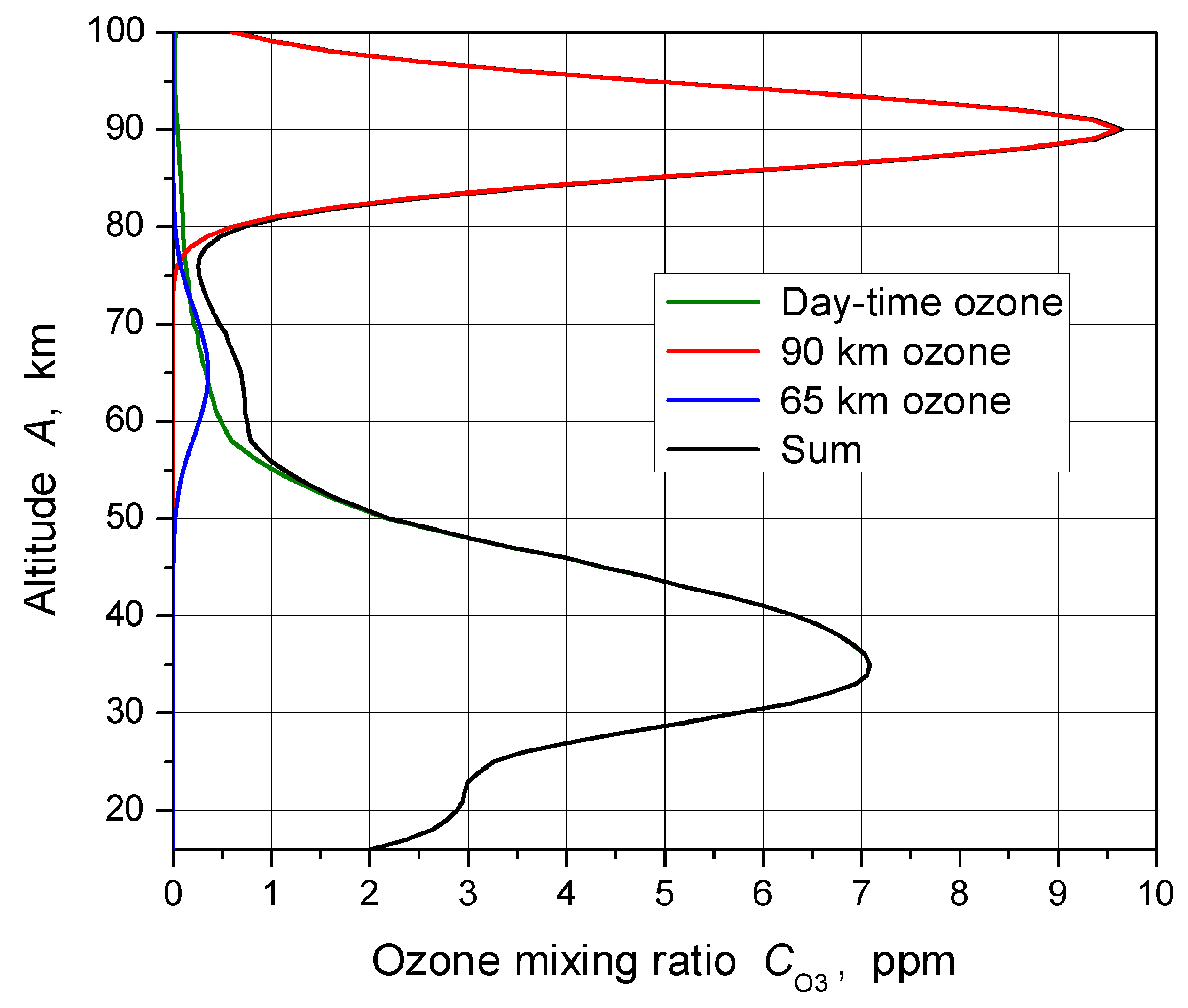
At night in the MLT region, ozone is not destroyed by solar radiation, and its content increases greatly. The secondary maximum in the OMR profile appears near 90 km in addition to its main stratospheric maximum at 30–35 km [
1,
2,
10]. Additionally, the tertiary OMR maximum may appear at night at altitudes of 60–70 km in polar and subpolar latitudes [
11]. Ozone observations at the MLT region are carried out mainly from satellites in optical (UV, visible, IR), submillimeter, and millimeter (microwave) ranges [
12,
13,
14,
15,
16,
17]. The most effective ground-based technique is remote sensing at microwaves [
18,
19,
20,
21,
22,
23]. The advantages of ground-based microwave remote sensing of ozone and other minor gases of the middle atmosphere are related to its relatively low dependence on weather conditions, wide altitude range and possibility of both day- and night-time observations.
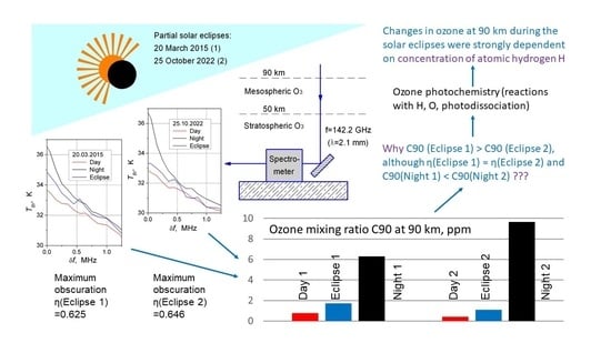
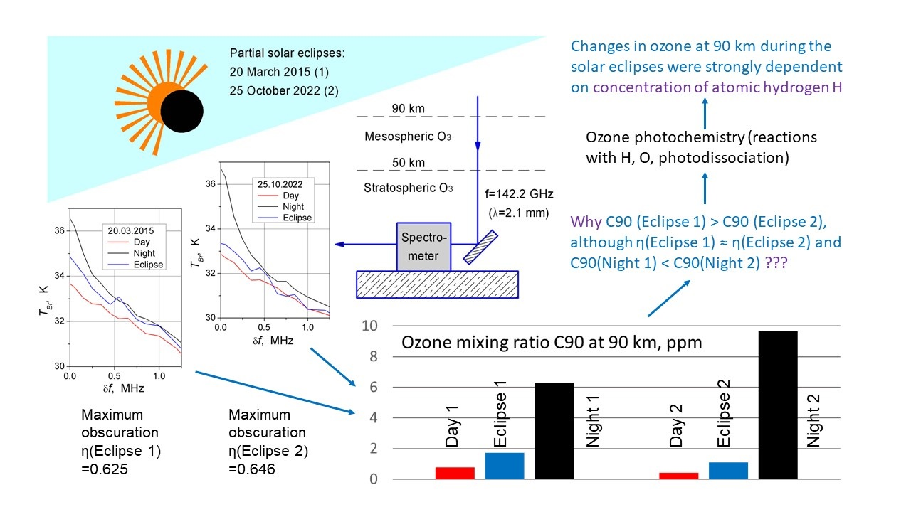
In this paper, we present and discuss the results of ground-based observations of mesospheric ozone over the Moscow region at a frequency of 142.2 GHz during the partial solar eclipses of 20 March 2015 and 25 October 2022. The main purposes of this work were to estimate changes in the OMR over the Moscow region during the eclipses and explain noticeable differences in the observational data obtained for the two events.
4. Observational Data
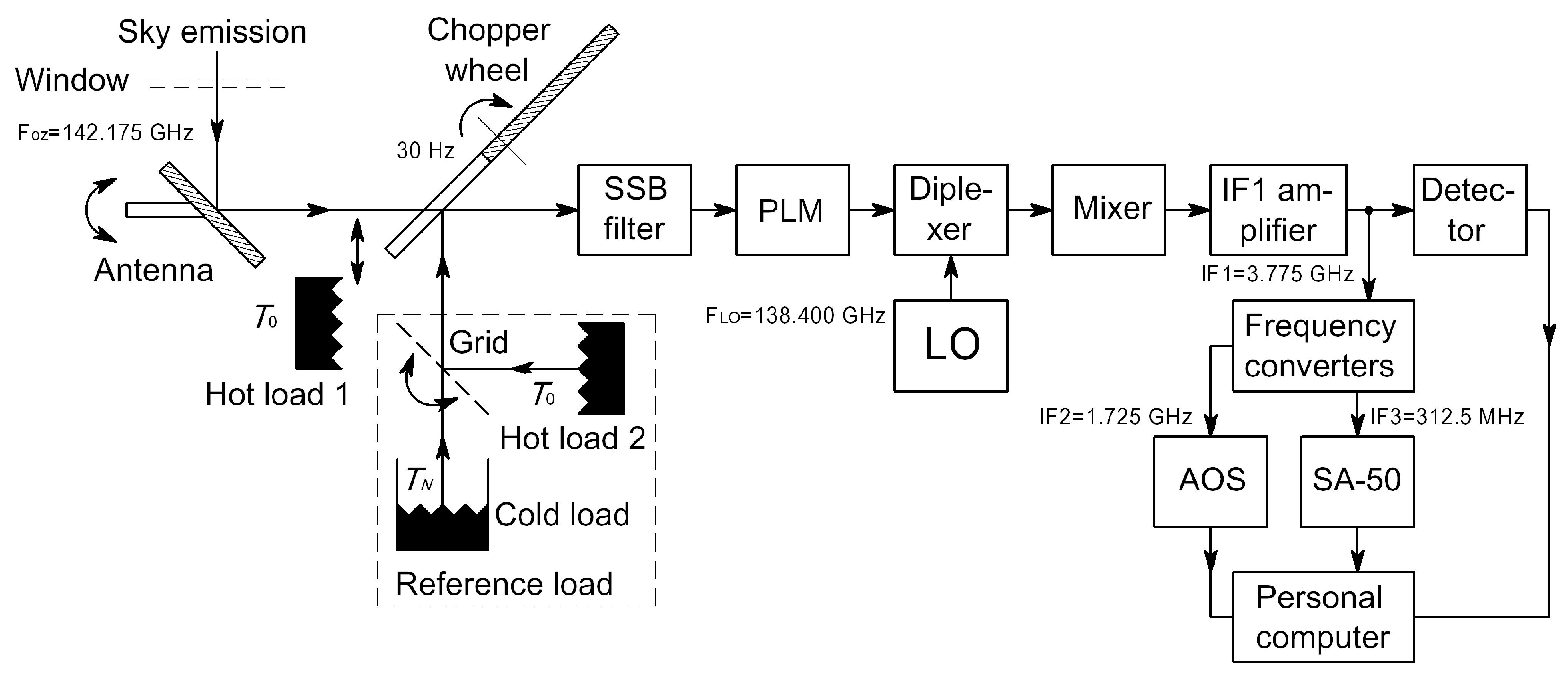
Measurements of mesospheric ozone with the MOS-4 in March 2015 were carried out on all nights from 15 to 20 March. The night measurements started shortly after the sunset at the ground level, continued throughout the night, and finished 0.5–1 h after the sunrise at the ground level. It allowed us to record both the night- and daytime ozone spectra. On 20 March, the measurements were continued in the daytime without turning off the spectrometer from 10:20 MT to 16:30 MT to cover both the solar eclipse and approximately two-hour time intervals before and after the eclipse. Thirty-three units of ozone spectra with an integration time of 200 s were recorded by the SA-50 during the eclipse. In March 2015, it was impossible to use the AOS and SA-50 simultaneously, and priority was given to the SA-50. On all the days from 13 to 20 March 2015, the weather was consistently clear, sunny, and stable, providing favourable conditions for the observations. During the solar eclipse of 20 March 2015, ground level temperature was +9 °C. The tropospheric loss in the eclipse culmination was estimated to be 1.84 dB for the antenna ZA = 60°.
On the contrary, in October 2022, the weather was not stable, and 25 October was a rare clear sunny day among cloudy and gloomy ones. The ground level temperature during the solar eclipse was +4°…+5 °C, lower than on 20 March 2015. This resulted in a decreased tropospheric loss of 1.48 dB in the eclipse culmination. Thus, the loss difference between the two eclipses was 0.36 dB (9%). On 25 October 2022, the observations started at 10:50 MT and were performed continuously until 22:15 MT. Thus, ozone spectra were recorded in the daytime before, during and after the solar eclipse as well as in the evening and in the night-time. A reduced measurement time of 80 s was used when recording the unit spectra on this day, and 89 unit of spectra were measured during the eclipse.
The average daytime ozone spectrum for 25 October 2022 (out of the eclipse period) measured by the MOS-4 in a frequency band of about 0.5 GHz is shown in
Figure 3. The spectrum is a fusion of the AOS and SA-50 spectra. It has a narrow central spike and broad wings. The shape of the ozone line corresponds to ozone emission from different layers of the stratosphere and the mesosphere, where pressure exponentially drops with increasing altitude. In this paper, our attention will be focused on changes in brightness temperature
TB around the ozone line peak during the solar eclipses and transitions from day- to night-time. Computer simulations [
21,
22] have shown that the main contributions to the line from ozone at altitudes above 60 km fall into frequency offsets δ
f from the line centre within approximately ±2 MHz.
It should be noted here that both the spectrum in
Figure 3 and all other spectra considered in this paper were corrected for tropospheric loss due to the absorption of microwaves in water vapour and molecular oxygen. The contribution from the water vapour and molecular oxygen to the experimental spectra and correspondent tropospheric loss were determined from the brightness temperature measured using the MOS-4 broadband detector. The contribution was subtracted from the spectra, and the residual (ozone line itself) was multiplied by the tropospheric loss. Thus, all the spectra in this paper are so-called “out-of-troposphere” ones.
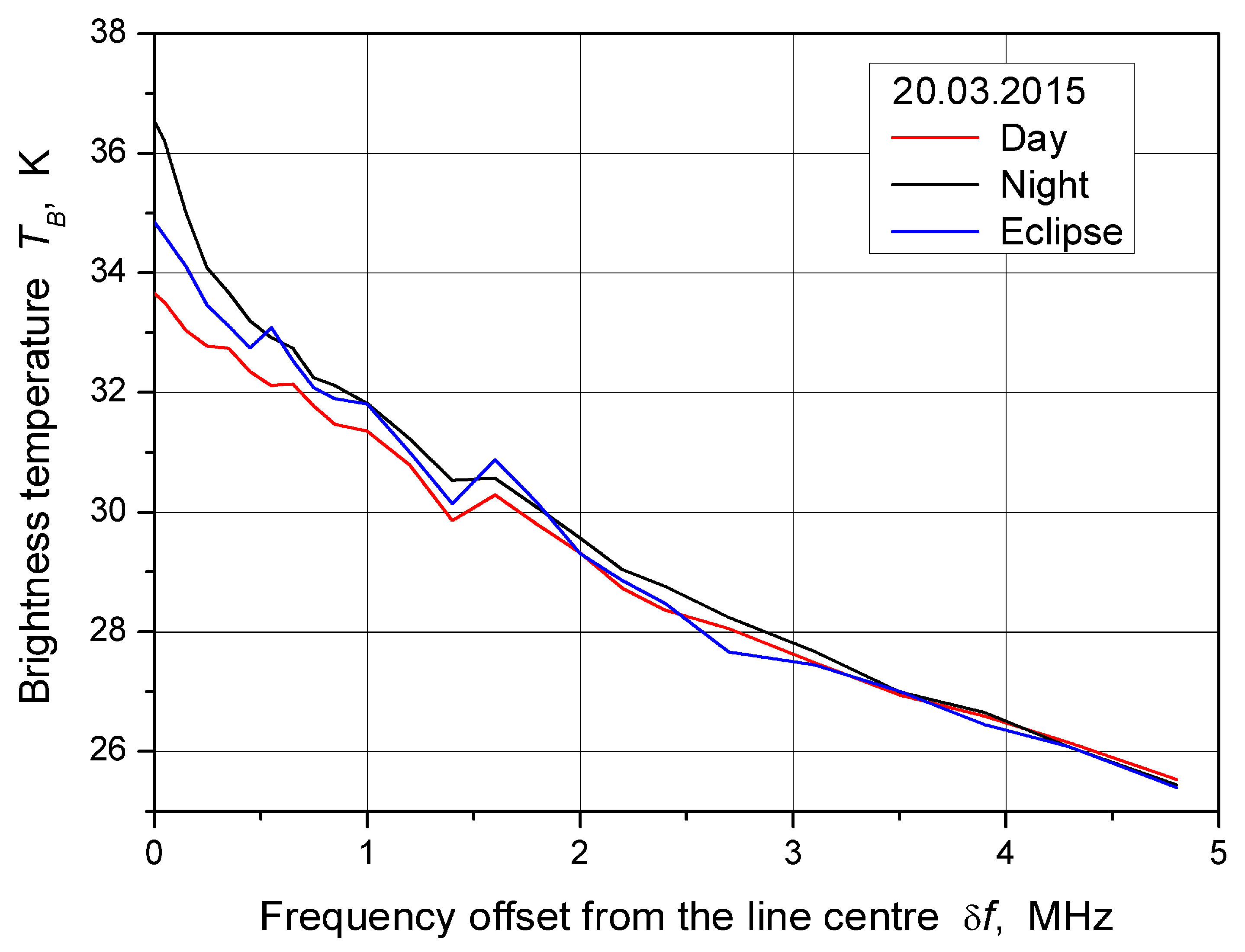
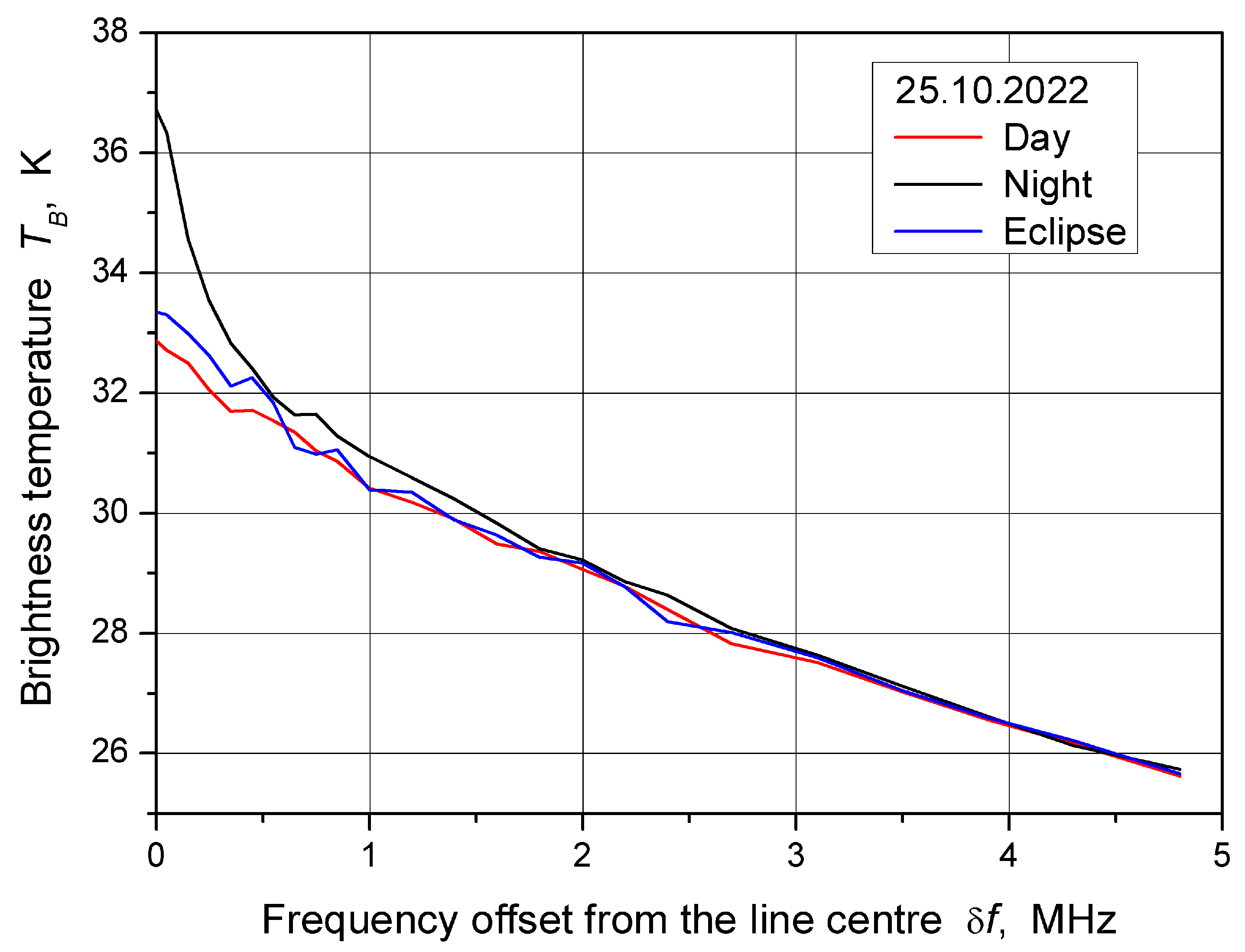
Changes in the ozone line spike for the solar eclipses are presented in
Figure 4 and
Figure 5. In these figures, red lines are daytime ozone spectra from the SA-50 just before and after the eclipses, blue lines are the spectra measured during the central third (33–67%) of the eclipses time, and black lines are average night-time spectra for the closest nights. The ozone line shown in
Figure 3 is symmetrical for frequency offsets up to several hundred megahertz. Thus, the spectra in
Figure 4 and
Figure 5 were obtained by folding their left and right wings to increase the signal-to-noise ratio by √2 times. The zigzag feature seen on the spectra in
Figure 4 at frequency offsets of around 1.5 MHz appeared as a result of detuning two channels in the SA-50. This malfunction was eliminated after technical maintenance and tuning of the device in 2016.
The unit spectra of the SA-50 measured during the eclipses were divided into several groups to obtain partial spectra for different phases of the eclipses (see
Section 5 for more details). It should be noted here that the noise levels of the partial spectra and accuracy of the OMR estimates from the spectra are inversely proportional to the root square of the total integration time of the spectra included in a group. Therefore, the number of parts into which the total eclipse time could be divided was limited by spectrometer noise.
It can be clearly seen through a comparison of
Figure 4 and
Figure 5 that the observed increase in the amplitude of the ozone line (the line amplitude is brightness temperature
TB (0) in the line centre at δ
f = 0) during the 20 March 2015 eclipse was significantly greater than during the 25 October 2022 eclipse. In fact, the difference between blue and red lines at zero frequency offset
TB (0, Eclipse)–
TB (0, Day) was 1.2 K on 20 March 2015 and only 0.5 K on 25 October 2022. Since the changes in the ozone line amplitude resulted from changes in mesospheric ozone content and distribution, this means that during the 20 March 2015 eclipse, the increase in mesospheric ozone was significantly greater than for the 25 October 2022 eclipse. As a result, the ratio was equal to 0.41 for 20 March 2015 and only 0.13 for 25 October 2022. Here,
TB (0, Night) is the amplitude of the average night-time ozone line. This discrepancy was surprising because the obscurations of the eclipses were close to each other (see
Figure 2). This fact was the main subject of further discussion in this paper.
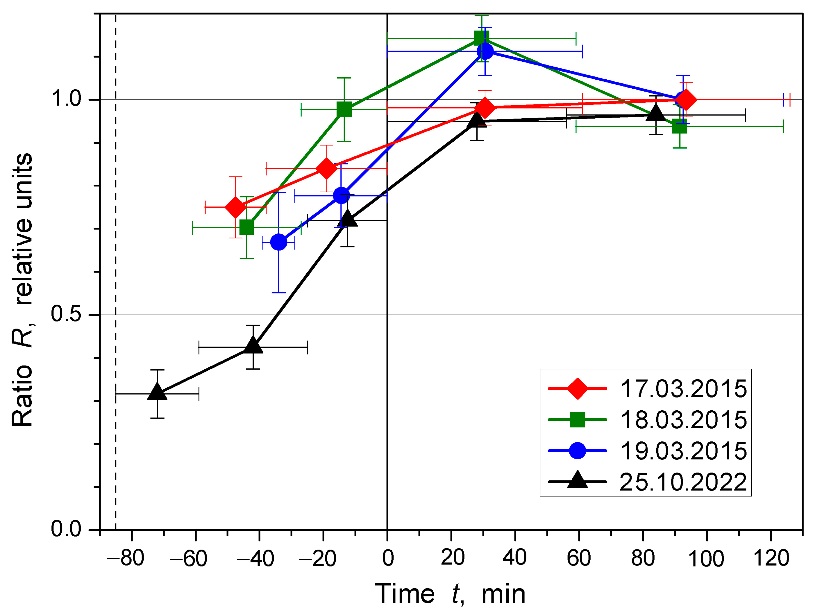
The similar ratio
was calculated for evenings of March 2015 and 25 October 2022 in dependence on time
t to see temporal changes in the ozone line amplitude during transitions from day- to night-time. In
Figure 6, the data are presented for the evenings of 17–19 March 2015 and 25 October 2022. Zero at the horizontal axis corresponds to sunset at an altitude of 100 km at the spectrometer line of sight, i.e., this point marks the disappearance of direct solar radiation at all altitudes lower than 100 km at the line. The vertical dashed line indicates the sunset at the ground level at the LPI. Numbers 0 and 1 at the vertical axis correspond to average day- and night-time amplitudes of the ozone line in accordance with the relation (2). The horizontal bars indicate time intervals of the observations, and the vertical bars denote errors calculated for the ratio
R(
t) based on the spectrometer noise corresponding to the intervals. It is seen from
Figure 6 that in the three evenings preceding the solar eclipse of 20 March 2015, the amplitude of the ozone line increased faster than in the evening of 25 October 2022.
5. Ozone Profiles
Collisional broadening of microwave spectral lines of ozone and other minor gases in the stratosphere and lower mesosphere is strongly dependent on pressure. This dependence is the key feature allowing for the retrieval of the altitude profiles of the species [
18]. At the LPI, ozone profiles are retrieved from the broadened 142.175 GHz ozone spectral line using an iterative algorithm based on Tikhonov’s method [
21,
22]. However, at altitudes above 60 km, the dependence of the ozone line width on pressure (on altitude) weakens because of the growing role of the Doppler broadening. Above 75 km, the Doppler broadening becomes greater than the collisional one. This results in a restriction on the maximum altitude up to which the ozone profile can be retrieved by the algorithm without using a priori information about the true shape of the profile [
21,
22]. Thus, additional data about the ozone profile at altitudes above 60 km is necessary for the profile retrieval both at night and during the solar eclipses.
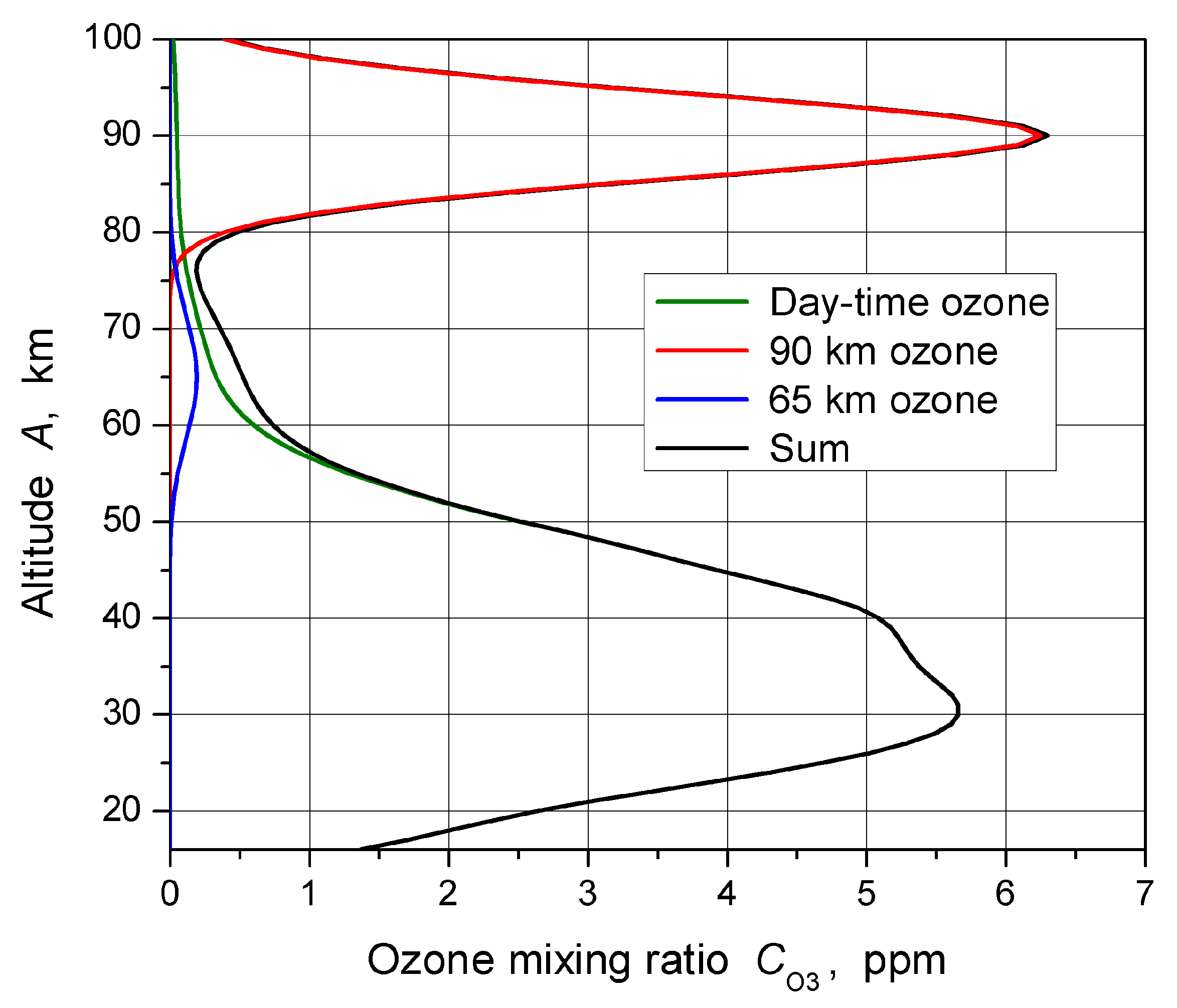
It was assumed in [
21] that the predominant part of the secondary night OMR maximum at an altitude of 90 km
C90 ≡
CO3 (
A = 90 km) was a Gaussian one with a 10 km full width at half maximum (FWHM). The amplitude of the Gaussian contribution must be slightly reduced compared to
C90 to take into account the small daytime OMR value, typically of order 0.1 ppm. Similarly, the night OMR value at 65 km
C65 ≡
CO3 (
A = 65 km) was assumed to be the sum of the daytime OMR at the altitude and the tertiary night maximum Gaussian contribution centered at 65 km with 15 km FWHM. Then, the a priori night OMR profile was built as the sum of the daytime ozone profile and the two night-time Gaussians. In [
21], the profile was used as the initial one for the following iterative retrieval procedure. However, it was found that the procedure practically did not change the ozone profile around 90 km, and noticeable changes appeared only at altitudes lower than 75 km. In this work, as will be seen from the further discussion, the most valuable information about mesospheric ozone variations during the solar eclipses was obtained only for altitudes around 90 km. Thus, we did not perform the full retrieval procedure for the OMR profiles during the night-time and time of the eclipse and used the above-described ozone profiles consisting of the three components.
The daytime ozone profiles for 20 March 2015 and 25 October 2022 retrieved using the iterative Tikhonov algorithm [
21,
22] are presented in
Figure 7 and
Figure 8 through the use of green lines. It should be noted that above 75 km, the profiles are close to the initial smooth reference profiles used in the retrieval procedure. To estimate the OMR values at altitudes of 90 and 65 km
C90 and
C65 at night-time and during the solar eclipses, we used a method initially proposed in [
21] and modified in [
23]. An experimental ozone spectrum
TB (δ
f) was compared with the model spectra
TB mod (
C90,
C65, δ
f) from the “out-of-troposphere” database calculated for some typical daytime ozone profile and a broad range of the OMR maxima values within
C90 = 0…20 ppm and
C65 = 0…5 ppm at the standard zenith angle ZA = 60° and a temperature of 206 K at an altitude of 85 km. Brightness temperatures of the ozone line in the database were calculated for the SA-50 frequency offsets δ
fi = 0, 0.05, 0.15, …, 0.85 MHz,
i = 1, 2, …, 10. In the method, the maxima
C90 and
C65 are determined as values minimizing the five-term quadratic form
where
and
are differences in brightness temperature between the neighbouring points with frequency offsets of δ
fi and δ
fi+1 for the folded experimental spectrum and the model spectrum. The largest frequency offset used in the form
Q is δ
f6 = 0.45 MHz. This means that Formula (3) takes into account all of the frequencies within the ±0.5 MHz band around the ozone line center. The computer simulations [
23] showed that the rms errors of the
C90 and
C65 values estimated using Formula (3) were proportional to the noise σ of the experimental ozone spectra at least for small σ < 0.1 K. Dependences of the OMR errors on the σ were found to be
where ξ
90 = 14 ppm/K and ξ
65 = 2.4 ppm/K. A significant increase in σ above 0.1 K may result in positive shifts (overestimation) of the calculated values of the OMR maxima
C90 and
C65 because of the appearance of non-monotonic parts on the experimental spectra. Slight non-monotonicity is noticeable in the blue curves in
Figure 4 (σ = 0.17 K) and
Figure 5 (σ = 0.15 K). For the correct determination of the “out-of-troposphere” σ values for the spectra shown in
Figure 3,
Figure 4 and
Figure 5, the spectrometer noise was multiplied by the same tropospheric loss as the ozone spectra themselves. Using the temperature of 206 K at an altitude of 85 km instead of its real values in the eclipse days estimated within 179–191 K (see
Section 6 for more details) could result in additional errors of the OMR values
C90 and
C65 within 10–15% [
21].
Using this method, the average night-time OMR values
C90 and
C65 were found. At an altitude of 90 km, the
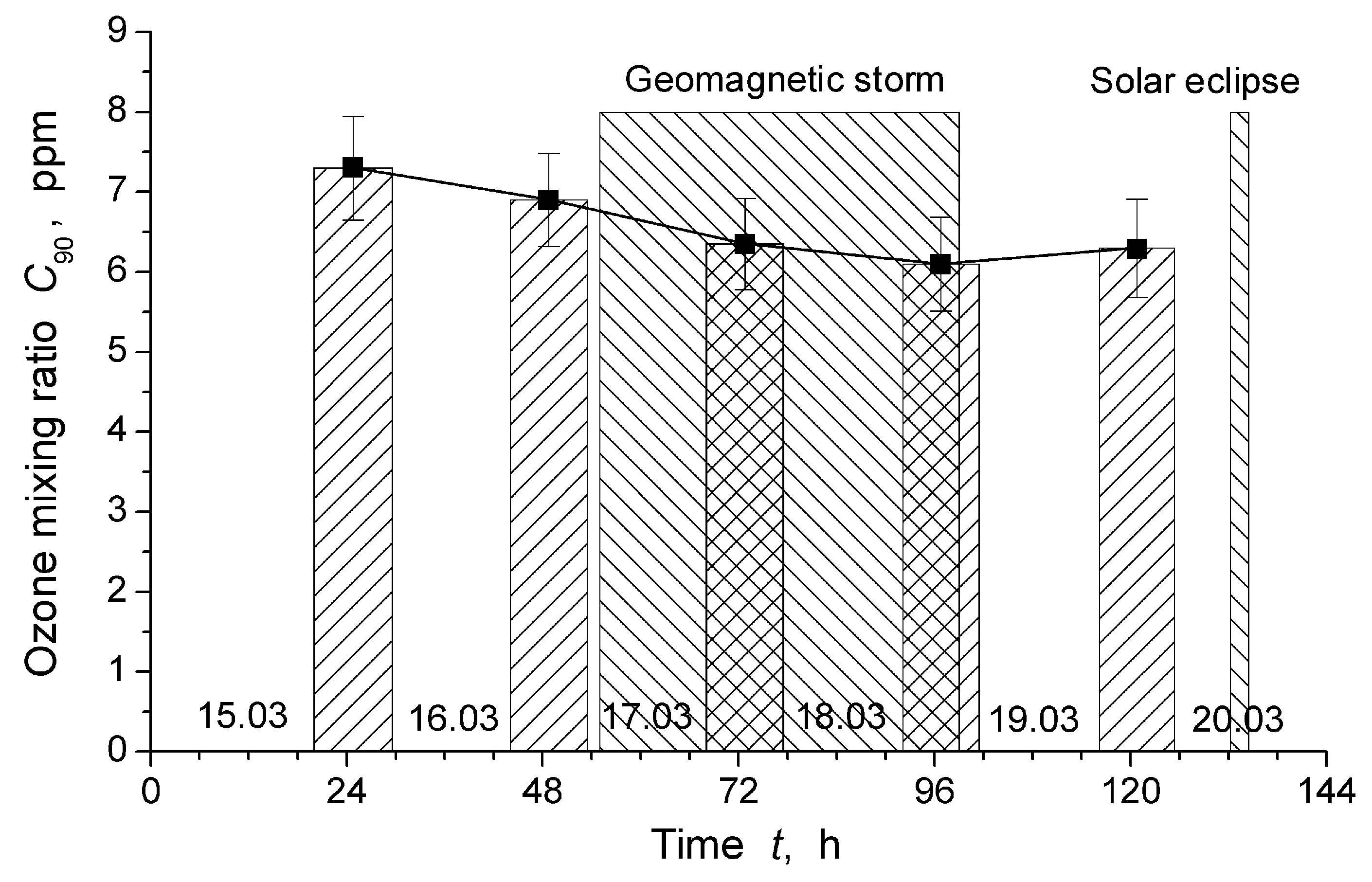
C90 was 6.3 ± 0.6 ppm in the night of 19–20 March 2015 and 9.65 ± 1.1 ppm in the night-time late on 25 October 2022. The increased rms error for 25 October 2022 was explained by the shorter observation time. The average OMR values at 90 km for all the nights from 15 to 20 March 2015 are presented in
Figure 9. The rms errors of the average night-time ozone spectra were σ ≈ 0.04 K. In accordance with relation (6), the calculated rms errors of the
C90 were σ
C90 ≈ 0.6 ppm. No strong changes in the OMR at 90 km during the St. Patrick’s severe two-step geomagnetic storm of 17–18 March 2015 [
26,
27] are seen in the figure. During the period of 15–20 March 2015, the average night OMR at 90 km smoothly varied between 7.3 and 6.1 ppm.
At an altitude of 65 km, the average night OMR C65 was 0.53 ± 0.1 ppm on the night of 19–20 March 2015 and 0.69 ± 0.2 ppm in the night-time late on 25 October 2022. On the other nights of 15–20 March 2015, the C65 varied within (0.53–0.74) ppm ± 0.1 ppm.
To study the changes in ozone content at 90 and 65 km during the eclipses, the sets of eclipse unit spectra were divided into groups in four ways and averaged in every group. The photochemical lifetime of ozone in the mesosphere is about 100 s [
1,
2], and this small delay in ozone response to changes in solar radiation flux was neglected. The first way (I) was to average all of the spectra for every eclipse. In the second way (II), the total eclipse time was divided into four equal parts,
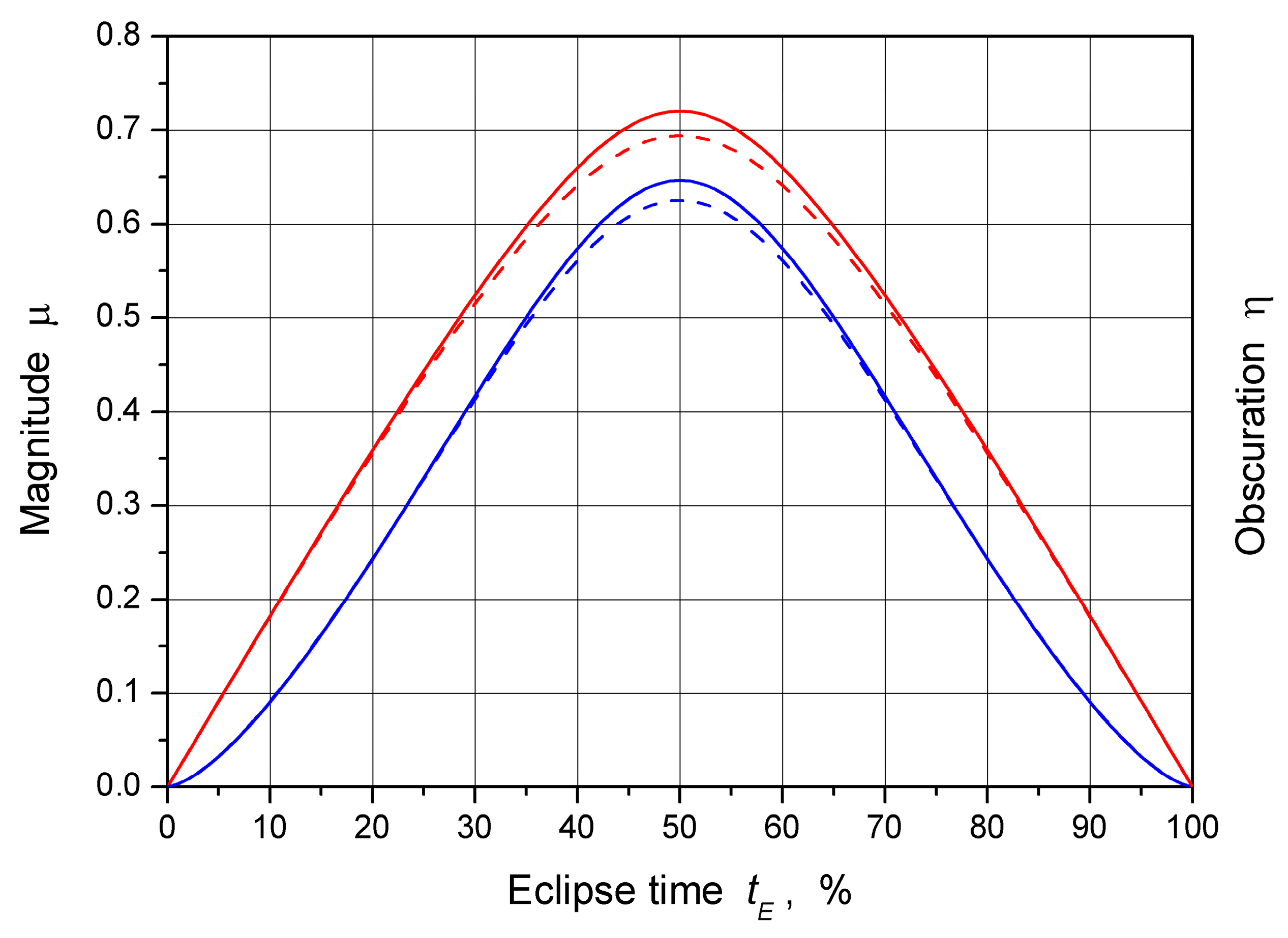
tE = (0–25), (25–50), (50–75), and (75–100). Hereafter the eclipse time
tE is expressed in percent, as in
Figure 2. It can be seen from
Figure 2 that the eclipse curves are symmetrical with respect to the culmination point
tE = 50%. Thus, the spectra falling into the first and fourth quarters contained identical information in terms of ozone, just like the spectra falling into the second and third quarters. For this reason, the spectra of these parts were united. The united groups were named (0, 25) and (25, 50) after the names of the first subgroups in every pair. Similarly, the groups in way (I) were named (0, 50) because, formally, it contained the spectra of two symmetrical parts,
tE = (0–50) and (50–100). In the third (III) and fourth (IV) ways, the total eclipse time was divided into six and eight equal parts,
tE = (0–16.7), …, (83.3–100) and
tE = (0–12.5), …, (87.5–100), respectively. After combining the unit spectra falling into parts symmetrical with respect to the point
tE = 50%, three and four groups were obtained for the ways. Similar to ways (I) and (II), these groups were named (0, 16.7), (16.7, 33.3), (33.3, 50) for the way (III) and (0, 12.5), (12.5, 25), (25, 37.5), (37.5, 50) for the way (IV). It should be noted that the total numbers of the unit spectra (33 for 20 March 2015 and 89 for 25 October 2022), in most cases, could not be divided into groups with quite equal numbers of spectra. Thus, the division was performed as accurately and reasonably as possible.
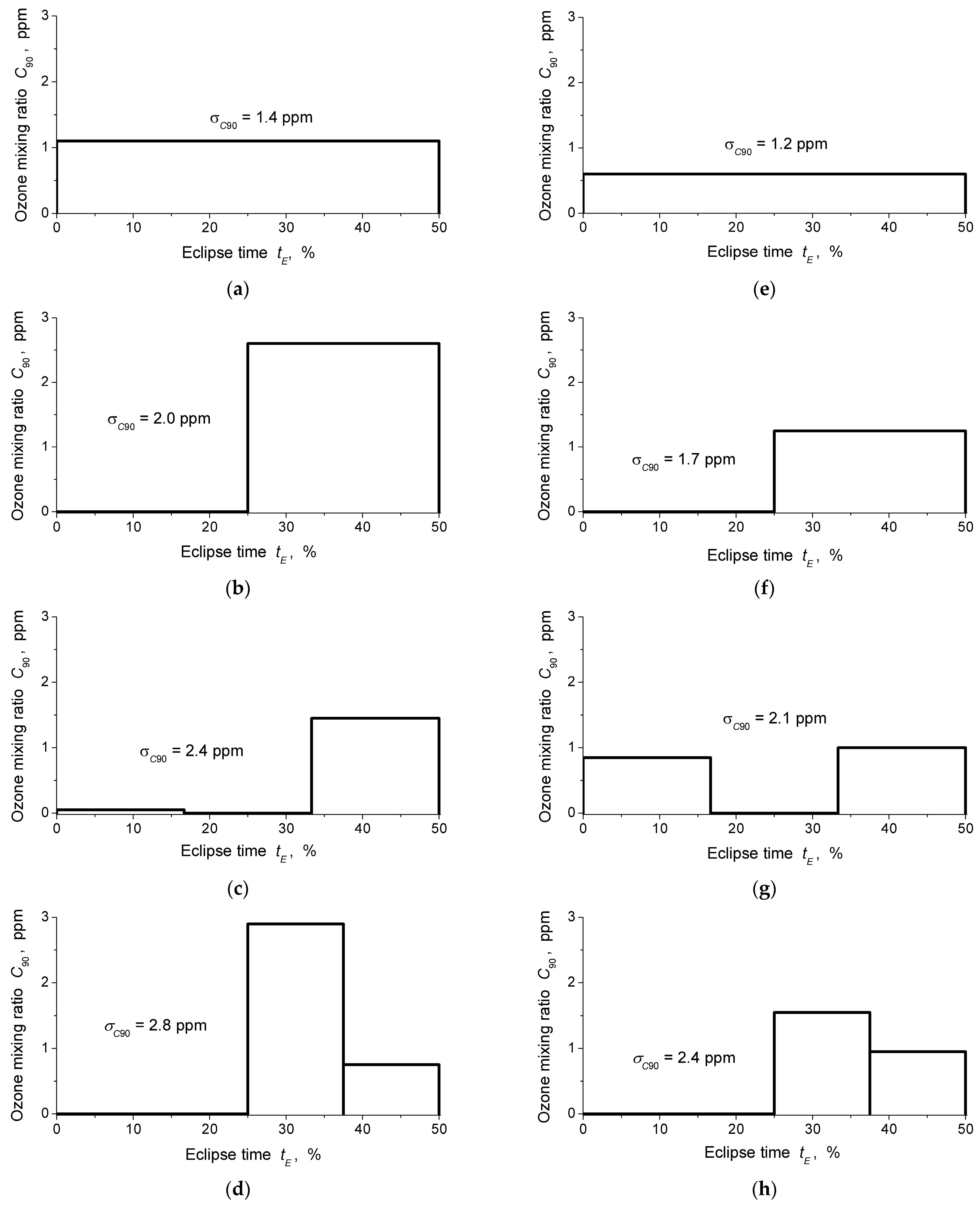
Then, the ozone mixing ratios
C90 (
tE1,
tE2) and
C65 (
tE1,
tE2) at altitudes of 90 and 65 km were found for all groups using the above-described method. Here,
tE1 and
tE2 are the time boundaries of the groups in percent. The OMR values at 90 km are presented in
Figure 10, together with estimates of their rms errors σ
C90 calculated using the relation (6). Successive rows of panels in
Figure 10 from top to bottom correspond to the division of the unit spectra by the ways from (I) to (IV). Data on the OMR
C90 (
tE1,
tE2) during the solar eclipse of 20 March 2015 are shown in the left column (panels a–d), and the same data on the eclipse of 25 October 2022 are presented in the right column (panels e–h). It is seen that the OMR in the left column, as a whole, is greater than that in the right one. This directly corresponds to the differences in the observed mesospheric ozone responses to the eclipses (see
Figure 4 and
Figure 5).
Additionally, it is noticeable in
Figure 10 that the rms errors σ
C90 are large and increase from the top to the bottom panels. The errors are inversely proportional to the root square of the number of the unit spectra in the groups. It is seen that on 25 October 2022, the errors were a little less than on 20 March 2015. This occurred because of two reasons. Firstly, the eclipse of 25 October 2022 lasted a little longer than the eclipse on 20 March 2015 (148 min versus 135 min), and secondly, the troposphere on 25 October 2022 was a little more transparent (loss of 1.48 dB, see
Section 4) than on 20 March 2015 (loss of 1.84 dB). Typically, at an altitude of 90 km, the errors σ
C90 were comparable or even exceeded the OMR values
C90 close to the eclipse culminations.
Unfortunately, those calculated by the groups’ OMR values C65 at an altitude of 65 km were not large and regular enough to reveal their dependences on the solar obscuration η. It was especially difficult since the expected dependence C65(η), in accordance with Formula (8), lower with exponent γ ≈ 0.5, was rather weak itself. For the solar eclipse on 20 March 2015, the OMR C65 (33.3, 66.7) was found to be 0.46 ± 0.42 ppm, but for the eclipse of 25 October 2022, it was estimated to be less than 0.2 ppm, with an rms error of 0.36 ppm. Thus, further in this paper, we discuss only ozone changes at an altitude of 90 km.
6. Discussion
M. Allen et al. [
2] have derived formulas for the ozone concentration at different layers of the MLT region. For altitudes of 50–80 km, the formulas can be used only in daylight hours, and at 90 km and above—they can be used around the clock. K. Imai et al. [
9] proposed a simplified form of the formula for ozone at altitudes between 50 and 70 km to present their data on the OMR profiles at the altitudes during the solar eclipse of 15 January 2010 in dependence on the Sun’s obscuration η
In accordance with [
2], at altitudes of 90 km and above, the concentration of ozone is equal to
Here,
J10 and
J11 are rates of ozone photodissociation due to the solar radiation with frequency ν
h is the Plank constant, [O], [O
2], [N
2], and [H] are concentrations of atomic and molecular oxygen, molecular nitrogen, and atomic hydrogen, respectively, and
k12–
k16 are rate constants of the ozone producing and destructive chemical reactions with these species:
These constants and their dependencies on temperature
T [
2] are listed in
Table 2.
The rate constants
k13 and
k14 are equal to each other (see
Table 2), but at 90 km, the concentration of atomic oxygen is much less than that of molecular oxygen: [O] << [O
2]. Thus, the first term in the parenthesis of the nominator in Formula (9) is small. Further, at altitudes of about 90 km, the contribution from the reaction (16) is 1–2 orders higher than one from the reaction (15). As a result, the next notations can be introduced:
and one can write Formula (9) in daylight hours as follows:
Here,
S is expressed in cm
−3 s
−1, while
J and
D are expressed as s
−1. The lifetimes of atomic hydrogen and oxygen at 90 km are of about 0.5 h and 1 week, respectively. The lifetimes highly increase above 90 km [
1,
2]. Molecular oxygen and nitrogen are stable components. At night the radiative term
J is equal to zero and
Provided that chemical term
D does not change noticeably from day to night, one can rewrite Equation (13) for daytime ozone concentration as follows:
Dividing the left and right parts of relation (21) by the total concentration of molecules in the air results in a formula for daytime OMR values:
The large night-time OMR maximum
C90 (Night) at an altitude of 90 km is well-defined from the microwave measurements (see
Figure 9) in contrast to ill-defined small daytime OMR values
C90 (Day) (typically
C90 (Day) < 1.2 ppm [
10]). Since the ratio
C90 (Night)/
C90 (Day) >> 1, the chemical term,
D, should be small,
D <<
J, as clearly seen from Formula (23). It follows from Formulas (17), (18) and (21) that the provided temperature and pressure are constant, and both the night-time ozone concentration and its mixing ratio at 90 km are proportional to the ratio of atomic-oxygen-to-atomic-hydrogen concentrations [O]/[H].
Similar to Equation (8), during the solar eclipses, the denominator in Formula (23) should be reduced because of the Sun’s obscuration:
An additional positive term,
B, was inserted into the denominator of Formula (24) to model the possible contribution of indirect (scattered and reflected) solar radiation to mesospheric ozone destruction. It was assumed that the term was small
B <<
J and constant during the eclipse because the scattered and reflected radiation could come from the regions far outside of the Moon’s shadow. At night, the term disappeared together with solar radiation
J. However, the transition from day to night for the indirect radiation could be completed later. Among the others, the term
B in Formula (24) turned out to be a suitable fitting parameter when analyzing the ozone data at 90 km. For convenience, we divided both the nominator and denominator in the right part of relation (24) by
J
to reveal the dependences of the OMR during the eclipses on the dimensionless ratios
BJ =
B/
J,
DJ =
D/
J, the above-mentioned night-time OMR values at 90 km
C90 = 6.3 ppm and
C90 = 9.65 ppm were used in Formula (25) for the eclipses of 20 March 2015 and 25 October 2022.
The solar eclipses of 20 March 2015 and 25 October 2022 were separated by a time interval of about 7.5 years and fell into different stages of two adjacent 11-year solar cycles. The first eclipse occurred at the decline of the 24th solar cycle, and the second—at the beginning of the 25th one. However, the F10.7 indexes of solar activity [
28] on the dates of eclipses were close to each other, 100.6 on 20 March 2015 and 103.6 on 25 October 2022. It was mentioned above that the solar zenith angles were different during the eclipses. The SZA varied from 57° to 60° on 20 March 2015 and from 68° to 75° on 25 October 2022. However, at altitudes of around 90 km, the atmosphere is sparse, and this difference could only slightly weaken the solar radiation on 25 October 2022, partly compensating for the difference in fluxes indicated by the F10.7 indexes. Thus, it was assumed that direct fluxes of solar radiation
J in Formulas (20), (22), and (23) were equal during the two eclipses. On the contrary, it seems possible that the increased SZA on 25 October 2022 could result in some increase in indirect radiation flux
B due to broadening the area where the reflection of solar radiation occurred at the sliding angles. However, any quantitative estimates of this effect are far from the scope of this paper.
To find dimensionless parameters
BJ and
DJ, which provide the best fitting of relation (25) to the experimental data
C90 (
tE1,
tE2) presented in
Figure 10, the parameters varied within sufficiently broad ranges of
BJ = −0.37…1 and
DJ = 0.025…0.3 to minimize the quadratic form of
F(
BJ,
DJ)
The number
N of terms summed up in the right part of Formula (26) increases from
N = 1 for way (I) to
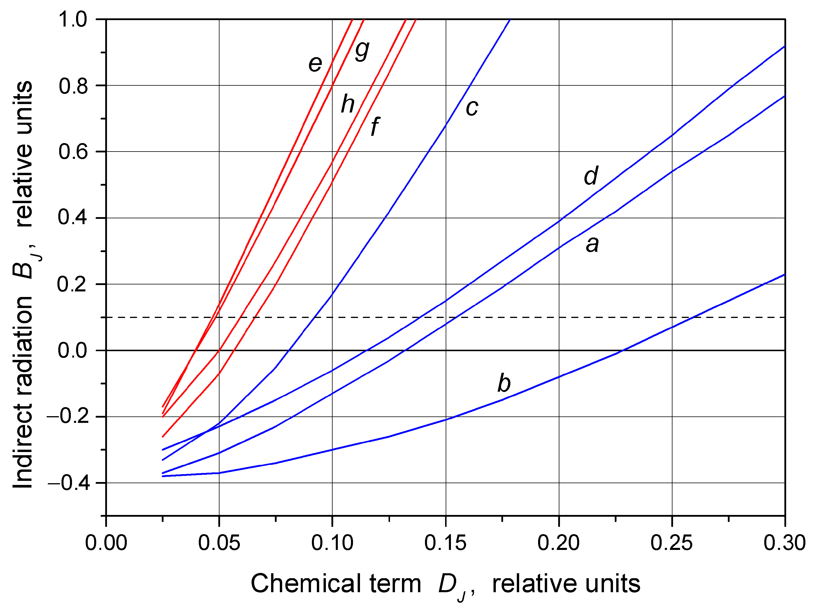
N = 4 for way (IV). Two sets of curves
BJ (
DJ) providing the fitting are presented in
Figure 11. The blue lines refer to the eclipse of 20 March 2015 and the red lines to the eclipse of 25 October 2022. The letters near the curves correspond to the notations of panels in
Figure 10. It can be seen that, despite the significant spread of the blue curves, they all move much to the right of the more compact set of red curves. This means that the magnitude of the chemical term
DJ in Equation (25) was much larger during the first eclipse. To estimate this term, we separately calculated for every curve
BJ (
DJ) and averaged through the blue and red sets of the curves the
DJ values for points where the curves crossed the levels
BJ = 0, 0.1, and 0.2. These small levels of indirect solar radiation seemed to be more or less realistic ones. It was found that for the eclipse of 20 March 2015,
DJ 20 was equal to 0.14, 0.16, and 0.18 for the three levels of
BJ. Similarly, the same values of the
DJ 25 for the eclipse on 25 October 2022 were 0.046, 0.055, and 0.064. As a result, the ratio of
DJ 20/
DJ 25 was found to be approximately constant for all three levels of
BJ and equal to 2.9–3.0.
Therefore, it was concluded that the magnitude of indirect solar radiation B, even if it differed from zero and was different for the two solar eclipses, had little effect on ozone variations at 90 km during the eclipses. Thus, the main reason for the strongly different observed responses of ozone at 90 km during the two eclipses with approximately equal obscurations of the Sun should have large differences in terms of the values of the chemical terms D and DJ in Formulas (24) and (25).
The error of ratio
DJ for every curve in
Figure 11 was estimated through the use of computer simulations performed at
BJ = 0. The rms errors σ
C90 of the OMR values
C90 shown in
Figure 10 were used in the simulations. As one might expect, these errors turned out to be large. They were lying within 0.21–0.26 for the blue curves a–d and within 0.11–0.13 for the red curves e–h, with some tendency in terms of decreased errors when there was an increase in
N from 1 to 4. For the blue and red curves, the errors were correlated because the same sets of unit ozone spectra were used for the calculation of
DJ at different
N. However, it was too difficult to model the errors of the average
DJ values. This would require varying the brightness temperatures in every channel of every unit spectrum for every eclipse. Thus, the errors of the average
DJ values at
BJ = 0 were estimated as falling in intervals (0.12, 0.24) on 20 March 2015 and (0.06, 0.12) on 25 October 2022, where the smaller numbers correspond to uncorrelated errors within the sets of blue and red curves, and the larger ones correspond to fully correlated errors. Despite the large errors, we believe that the data shown in
Figure 11 quite clearly discriminated the values of the
DJ for the two solar eclipses.
Three possible explanations for the three-times difference in the magnitudes of the chemical term D for the two solar eclipses were considered:
(1) The severe geomagnetic storm of 17–18 March 2015 [
26,
27] could have noticeably accelerated the chemical destruction of ozone in the upper mesosphere because of the increased HO
x content (mainly atomic hydrogen H) and NO
x (mainly nitric oxide NO) radicals resulting from the ionization of the upper mesosphere by charged particles of solar plasma [
3,
4,
27]. Excessive atomic hydrogen should have disappeared after several hours [
1,
4], but the lifetime of mesospheric NO is about 2 days [
1]. Thus, the increase in NO content could have been partially maintained by 20 March 2015 and ozone destruction in the reaction
could increase the chemical term
D by the time of the solar eclipse on 20 March 2015. However, any strong decrease in night ozone was not seen at 90 km after 16 March 2015, as shown in
Figure 9. The night-time OMR
C90 (Night) decreased by 8%, from 6.9 ppm on the night of 16–17 March, just before the geomagnetic storm, to 6.35 ppm on the night of 17–18 March during the storm. Then, the decrease in ozone content slowed down to 6.1 ppm on the night of 18–19 March and was replaced by a slow increase up to 6.3 ppm on the night of 19–20 March. Therefore, the geomagnetic storm did not significantly increase the chemical term
D at an altitude of 90 km on 20 March 2015. Possible changes in
D resulted from the storm hardly exceeding approximately 10%. It should also be noted that the maximum destruction of ozone by NO molecules is located lower, at altitudes of about 80 km [
3,
4], and ozone at 90 km is less sensitive to possible increases in NO content;
(2) The rate constants
k12–
k16 of chemical reactions (12)–(16) are temperature-dependent (see
Table 2) [
2]. The reaction (15) has a very strong dependence on temperature, but it plays only a minor role in ozone destruction at altitudes of about 90 km. The highest points of the temperature profiles available from the ERA5 reanalysis database [
29] are located at altitudes of about 78 km. On 20 March 2015, the upper temperature points of the profile were 200.53 K at 78.09 km and 212.83 K at 72.43 km. Similarly, on 25 October 2022, the values were 192.71 K at 77.63 km and 201.21 K at 72.21 km. All the data referred to 12:00 MT. Linear interpolation of the ERA5 temperature profiles to the lower mesopause altitude of 85 km resulted in temperatures of about 183 K and 179 K for the two dates. Otherwise, spline interpolation of the ERA5 profiles using the average model temperature of 191 K at an altitude of 100 km [
30] resulted in temperatures at 90 km of 191 K on 20 March 2015 and 179 K on 25 October 2022. According to
Table 2, the increase in temperature by 12 K from 179 K to 191 K results in an increase in
D by 9% and a decrease in
S by 19%. For the smaller temperature increase of 4 K, the increase in
D is only 3%, and the decrease in
S is 6%. Obviously, the temperature dependence of the chemical term
D is too small to explain the change by approximately three times in terms of magnitude;
(3) Then, it remains only to assume that the main reason for the large difference in the magnitudes of
D was the significantly lower concentration of atomic hydrogen H at altitudes of about 90 km on 25 October 2022 in comparison with 20 March 2015. Taking into account that the above-discussed temperature effects were small, the hydrogen concentration should have decreased by almost three times. This assumption seems consistent with the results of modeling the distribution of atomic hydrogen in the mesosphere presented in [
1]. In that book, at latitudes of about 60°, the calculated concentration of atomic hydrogen at 90 km in summer was considerably higher than in winter (approximately 10
8 cm
−3 versus 3 × 10
7 cm
−3). These seasonal variations depend on both eddy transport and photochemical processes [
1,
2]. Since 20 March 2015 was close to the vernal equinox, but 25 October 2022 was more than a month later than the autumnal equinox, we can assume that the concentration of atomic hydrogen in the second case could be lower.
Substituting the average values of
DJ = 0.14 for 20 March 2015 and
DJ = 0.046 for 25 October 2022 into Formula (25) at
BJ = 0, we obtained the daytime OMR values of (out of the eclipse time)
C90(Day) at an altitude of 90 km for the dates. They were at 0.77 and 0.42 ppm, respectively. Similarly, the calculated OMR values at the eclipse culminations
C90(η
max) were 1.71 ppm on 20 March 2015 and 1.11 ppm on 25 October 2022. The values satisfactorily matched the data in relation to
C90(η) presented in
Figure 10. It is interesting to note that the ratio of
C90(η
max)/
C90(Day) was equal to 2.2 on 20 March 2015 and 2.6 on 25 October 2022. This means that relative changes in ozone at 90 km during the second eclipse were even greater, but they could not be detected with sufficient accuracy because of spectrometer noise.
Thus, the observed change in the ozone content (concentration or OMR) at an altitude of 90 km during a solar eclipse depends mainly on the night-time ozone content and on the concentration of atomic hydrogen at this altitude, determining the chemical term D in Formula (24). For partial solar eclipses with obscuration η < 1 − DJ2, the greater the concentration of atomic hydrogen, the greater the absolute increase in ozone content during the eclipse. (For values DJ < 0.2 found in this work the rule should be correct for all eclipses with η < 0.96). On the contrary, relative changes in the ozone content during any eclipse will increase with a decrease in atomic hydrogen concentration because of the decrease in daytime ozone content.
Additionally, the changes in the magnitude of the chemical term
D allowed us to explain the differences in the transition curves from day to night presented in
Figure 6. Let us use Formula (24) at
B = 0 for the evening time as well. Then, the factor (1 − η) corresponds to the reduction in solar flux
J during sunset. It can be seen from (24) that the smaller the
D, the less sunlight should remain; therefore, the OMR
C90 approaches its night value
C90 (Night). Therefore, on the evening of 25 October 2022, at a low value of
D, the transition to night conditions occurred later than on the evenings of 16–18 March 2015. An alternative explanation of the differences in the transition curves for March 2015 and 25 October 2022 is the assumption of a much larger amount of indirect radiation flux
B on the evening of 25 October 2022. However, this requires unrealistically large values
B > 0.2
J. Therefore, such an explanation seems unlikely.
7. Conclusions
In this work, we observed microwaves and studied variations in mesospheric ozone O3 over the Moscow region during two partial solar eclipses on 20 March 2015 and 25 October 2022. Both eclipses occurred at midday, with clear weather favourable for observations. The maximum obscuration of the Sun during the eclipses was 0.625 on 20 March 2015 and 0.646 on 25 October 2022. The brightness temperature of the 100,10–101,9 rotational ozone spectral line centered at 142.175 GHz was measured with a frequency resolution of 0.1 MHz near the line center by the ground-based low-noise spectrometer MOS-4 located at the LPI in Moscow. The unit ozone spectra with durations of 200 or 80 s were recorded before, during, and after the eclipses. The spectra were corrected for the tropospheric loss estimated from the measured average brightness temperature of the sky in a broad band of 0.6 GHz. Then, the spectra recorded within the eclipse time were divided into groups with different durations and averaged by the groups to reveal the dependence of the ozone mixing ratio (OMR) in the mesosphere on the obscuration of the Sun at altitudes of 90 and 65 km, where the secondary and tertiary maxima of the OMR profile are located. Special techniques were used to calculate the OMR values of C90 and C65 at these altitudes. It was surprising that despite the close values of the maximum eclipse obscurations, the increases in both brightness temperatures of the ozone line and in the OMR values at 90 km were approximately two times greater on 20 March 2015 than on 25 October 2022.
Unfortunately, the calculated OMR values of C65 at an altitude of 65 km were not large and regular enough to reveal their dependence on solar obscuration. For the solar eclipse on 20 March 2015, the C65 value for the central third of the eclipse time was found to be 0.46 ± 0.42 ppm, but for the eclipse of 25 October 2022, it was estimated to be less than 0.2 ppm, with an rms error of 0.36 ppm.
To understand the origin of the large difference in results at 90 km, the formulas for ozone content in the mesosphere derived by M. Allen et al. [
2] were used. Their formula for ozone concentration at altitudes of 90 km and above was modified for use with the OMR values during solar eclipses. Fitting the modified formula to the calculated
C90 values resulted in the conclusion that on 25 October 2022 at 90 km, the relative role of the chemical destruction of ozone (compared with its photodissociation by solar radiation) was approximately three times less than on 20 March 2015. Thus, at approximately equal solar fluxes, we had to conclude that absolute rates of the chemical ozone destruction, mainly by atomic hydrogen, differed by three times for the two eclipses.
Night-time measurements of the mesospheric ozone from 15 to 20 March 2015 showed the possibility that the increase in chemical ozone destruction resulted from the severe geomagnetic storm of 17–18 March 2015 preceding the solar eclipse on 20 March 2015, which did not exceed approximately 10% at an altitude of 90 km. Similarly, an estimated decrease in temperature at altitudes of around 90 km within 4–12 K on 25 October 2022 compared to 20 March 2015 could not decrease the rate constant of the reaction of ozone with atomic hydrogen by more than 9%. Consequently, the most probable reason for the three-fold difference in chemical ozone destruction rates was a decrease by almost three times in atomic hydrogen concentration on 25 October 2022 in comparison to 20 March 2015.
Using the modified formula for the OMR at 90 km, we calculated the daytime OMR values C90(Day) (out of the eclipse time) of 0.77 and 0.42 ppm, respectively, for 20 March 2015 and 25 October 2022. At the eclipse culminations, the calculated OMR values C90(ηmax) were 1.71 ppm on 20 March 2015 and 1.11 ppm on 25 October 2022. Thus, the ratio C90(ηmax)/C90(Day) was equal to 2.2 on 20 March 2015 and 2.6 on 25 October 2022. This means that relative changes in ozone at 90 km during the eclipse of 25 October 2022 were even greater, but they could not be detected with sufficient accuracy because of spectrometer noise.
Thus, the observed changes in the ozone content (concentration or OMR) at an altitude of 90 km during a solar eclipse depend mainly on the night-time ozone content and on the concentration of atomic hydrogen at this altitude. For partial solar eclipses with obscuration η < 1 − DJ2, the greater the concentration, the greater the absolute increase in the ozone content during the eclipse. Otherwise, relative changes in the ozone content during any eclipse will increase with the decrease in the atomic hydrogen concentration. Additionally, the decrease in the rate of chemical ozone destruction results in a later transition from day to night in the mesospheric ozone profile.
The research confirmed that solar eclipses provide unique possibilities for experimentally studying the photochemistry of mesospheric ozone and testing photochemical models. Interesting events, such as sufficiently deep partial and, especially, total solar eclipses, are rare in one place. In Moscow, the next eclipse comparable in the Sun’s obscuration to the eclipses discussed in this paper will not occur until 2039. Probably, microwave spectrometers operating onboard satellites have more chances to observe and investigate the changes in mesospheric ozone profiles during solar eclipses.


