Mapping Surface Features of an Alpine Glacier through Multispectral and Thermal Drone Surveys

Abstract

Glacier surfaces are highly heterogeneous mixtures of ice, snow, light-absorbing impurities and debris material. The spatial and temporal variability of these components affects ice surface characteristics and strongly influences glacier energy and mass balance. Remote sensing offers a unique opportunity to characterize glacier optical and thermal properties, enabling a better understanding of different processes occurring at the glacial surface. In this study, we evaluate the potential of optical and thermal data collected from field and drone platforms to map the abundances of predominant glacier surfaces (i.e., snow, clean ice, melting ice, dark ice, cryoconite, dusty snow and debris cover) on the Zebrù glacier in the Italian Alps. The drone surveys were conducted on the ablation zone of the glacier on 29 and 30 July 2020, corresponding to the middle of the ablation season. We identified very high heterogeneity of surface types dominated by melting ice (30% of the investigated area), dark ice (24%), clean ice (19%) and debris cover (17%). The surface temperature of debris cover was inversely related to debris-cover thickness. This relation is influenced by the petrology of debris cover, suggesting the importance of lithology when considering the role of debris over glaciers. Multispectral and thermal drone surveys can thus provide accurate high-resolution maps of different snow and ice types and their temperature, which are critical elements to better understand the glacier’s energy budget and melt rates.

1. Introduction

Under ongoing climate change, glacier retreat in the Alps is occurring at unprecedented rates [1,2]. Besides changes in climate conditions (e.g., changes in atmospheric temperature and precipitation amounts and phase), several other factors, such as the snow and ice albedo, liquid water, amount and composition of light-absorbing impurities deposited on the snow and ice, and supraglacial debris, can affect the mass balance of mountain and debris-covered glaciers [3].

Tongues of retreating glaciers display very low albedo values (<0.4), and a gradual lowering of the albedo has been observed in recent decades [4]. This is due to coverage of the ice by layers of debris [5,6], the accumulation of impurities during the ablation season (e.g., cryoconite) [7,8] and the unveiling of darker firn bands from previous years [9]. During summer, large portions of the Alpine glaciers are snow-free and an increasing amount of dark bare ice and firn is exposed to solar radiation, having a substantial impact on the amount of energy absorbed by glacier surfaces [10].

The snow and glacier ice reflectance, often in the form of a glacier-wide broadband surface albedo, is a key parameter in the mass and energy balance of glaciers because it controls the shortwave radiation budget and consequently affects glacier melting [11,12,13]. However, only few studies have quantified the spatial and temporal variability in bare-ice reflectance in the ablation zones of mountain glaciers [14].

The assimilation of spatially distributed bare-ice glacier albedo in mass-balance modelling can significantly improve the results [15]. In fact, glacier albedo values lower than 0.34 (value often used in glacier modelling for bare ice) can significantly modify the surface energy balance and induce melting [16,17,18,19].

Debris cover, besides affecting snow and glacier ice reflectance, strongly influences the thermal properties of a glacier. While sparse debris cover enhances ice melt due to the darkening of the glacier surface [20,21,22], debris cover thicker than a few centimeters preserves the underlying ice from melting, acting as an insulator [23,24].

To quantify the spectral variability of surface reflectance and albedo of mountain glaciers, as well as to characterize the spatial distribution and thickness of debris cover, increasing studies are focusing on the retrieval of glacier optical and thermal properties from relatively high-spatial-resolution remotely sensed data [10,17,25,26].

During the last few years, drone surveys have been widely applied in glaciology [27,28], both in mountain [29,30] and in polar [31] areas. In fact, drones offer the possibility to perform repeated surveys at high spatial and temporal resolutions, enhancing our ability to monitor rapidly changing environments and landscape features [32,33,34], as in the case of glacial environments. While the application of drone photogrammetry provides important information regarding glacier mass change and dynamics [35,36], only few studies have made use of multispectral [37,38,39] and thermal drone surveys [40,41,42]. Tedstone et al. [37] used a multiband camera to map glacier algae and weathering crust in Southwest Greenland. Kraaijenbrink et al. [41] exploited drone thermal data to map the surface temperature of a debris-covered glacier in the central Himalayas. Forte et al. [40] recently discriminated debris cover and rock outcrops from bare ice using a thermal drone survey. Furthermore, other studies [43,44,45,46] recently suggested that the thickness of glacier debris cover can be estimated from drone thermal measurements.

In the European Alps, no fine-scale mapping (<1 m) of glacier surface properties has been performed so far using combined multispectral and thermal drone surveys. As a contribution to this knowledge gap, we present a study of the ablation zone of the Zebrù glacier, located in the Central European Alps, by using optical and thermal data collected from field and drone platforms to map the abundances of predominant glacier surfaces (i.e., snow, clean ice, melting ice, dark ice, cryoconite, dusty snow and debris cover). Moreover, we map the glacier surface temperature using spatially resolved emissivity maps derived from the multispectral survey, and we evaluate the potential of surface temperature in characterizing debris-cover thickness.

2. Materials and Methods

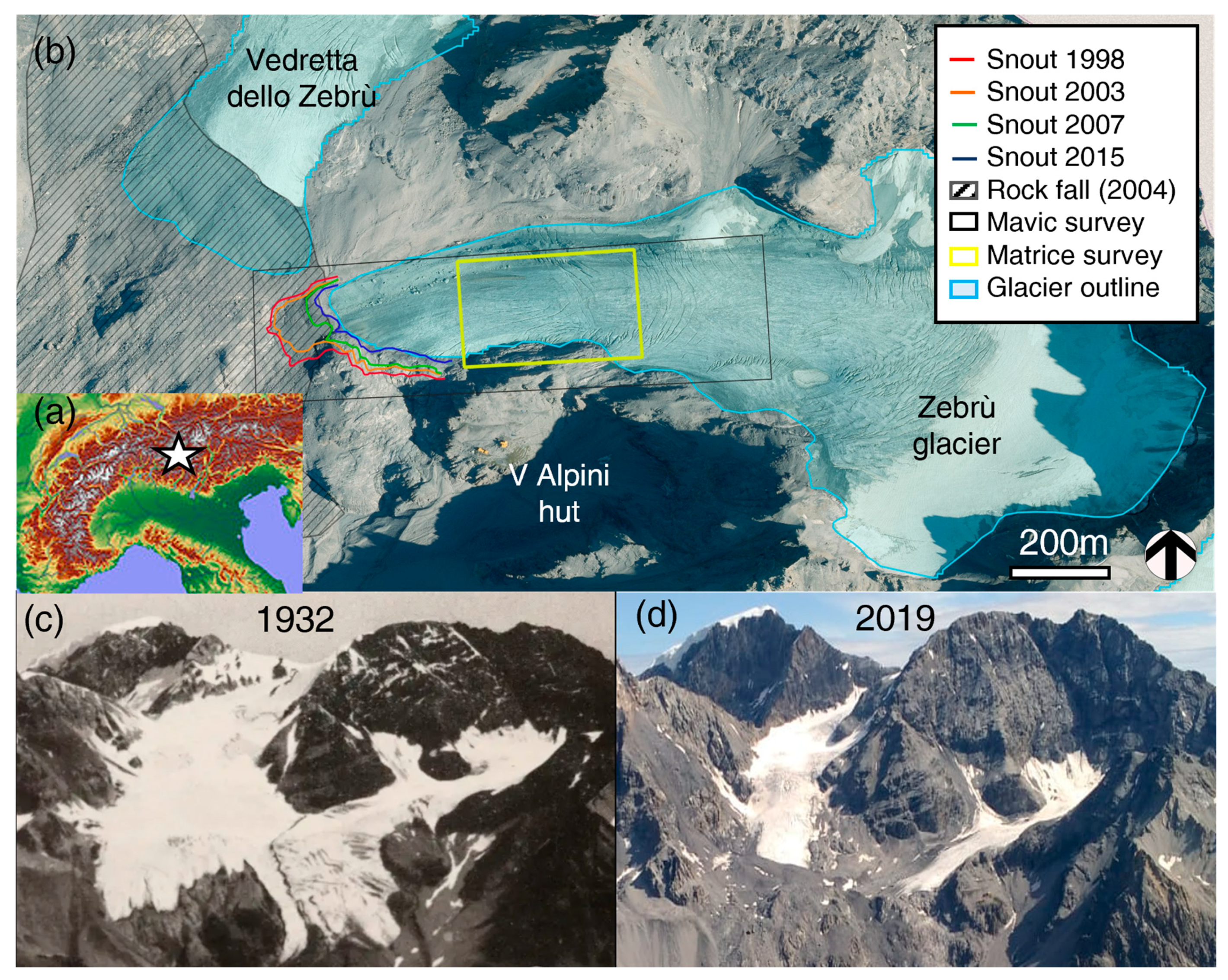
2.1. Study Area

The Zebrù glacier (46°29′05″N, 10°32′20″E) is a typical Alpine valley glacier located in the Ortles-Cevedale group in the Southern Rhaetian Alps (Central Italian Alps, Italy) (Figure 1). The glacier is part of a glacier complex consisting of two distinct sectors: the Zebrù glacier (also referred as Eastern sector) and the Vedretta dello Zebrù (also referred to as Western sector) [47]. The two sectors are fed by distinct accumulation basins. While the two glaciers were once connected, they have been progressively separating in recent decades. On 18 September 2004, the Zebrù valley was affected by a massive rock avalanche (~3 million m³) that covered part of the Vedretta dello Zebrù [48]. The Eastern sector was only marginally affected by the event.

The ablation area of the Zebrù glacier extends for about 250 m in width and about 1 km in length, with an elevation ranging between 2900 m and 3100 m above sea level. The glacier is surrounded by relatively high peaks, such as Monte Zebrù (Cima South-East; 3724 m and North-West 3735 m), Punta Thurwieser (3641 m) and Gran Zebrù (3857 m).

In Figure 1, the two sectors of the Zebrù glacier are displayed. The position of the Zebrù glacier snout was manually digitized from aerial photos collected in 1998, 2003, 2007 and 2015 (Regione Lombardia). Both glaciers suffered a steady retreat in the last few decades. Figure 1c,d shows a visual comparison between a picture acquired in 1932 and one acquired in 2019 from Monte Confinale.

2.2. Drone Platforms and Instruments

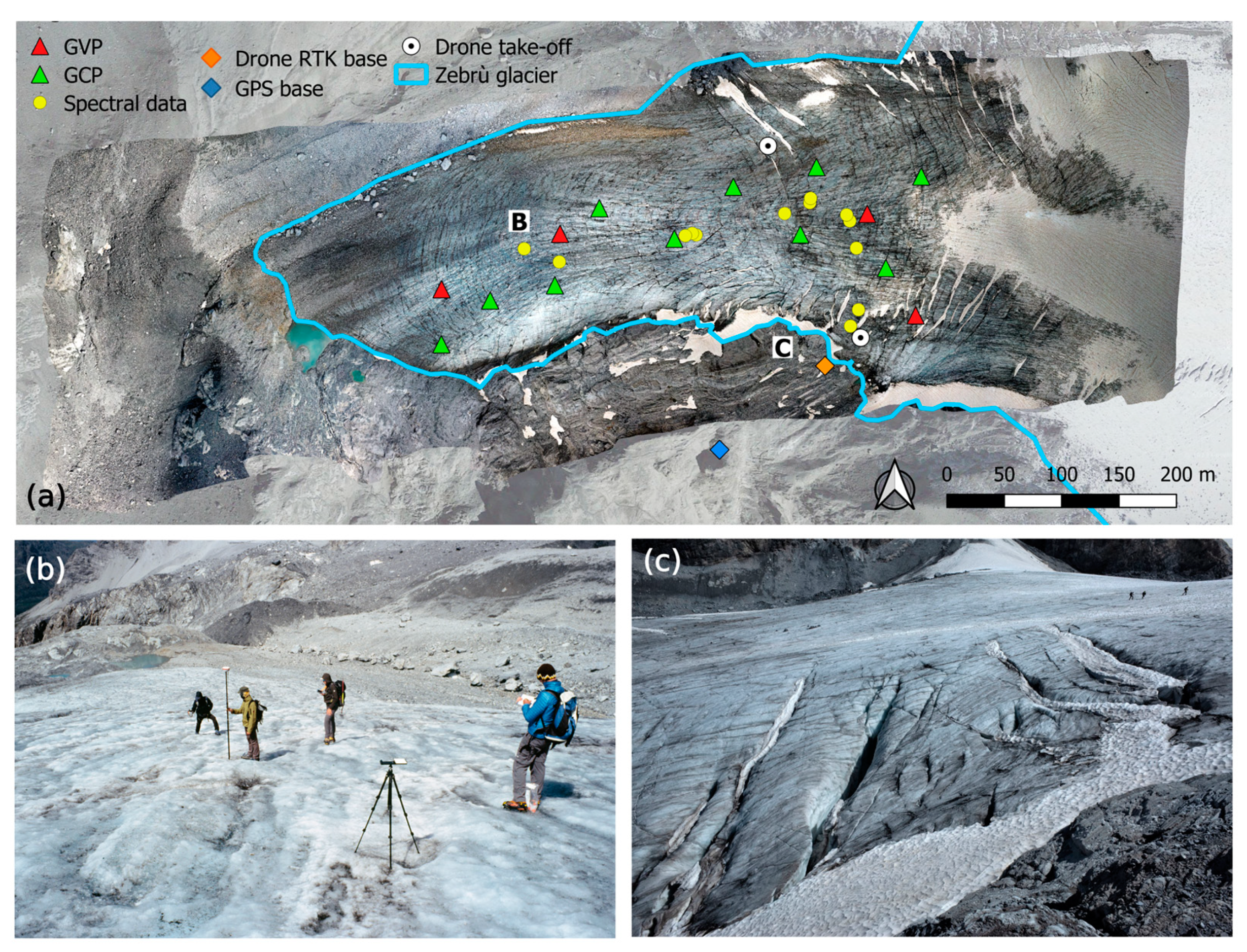
The drone surveys (

Table 1. Flight plan settings for RGB, multispectral and thermal infrared (TIR) image acquisitions.

Image Type	Lateral Overlap	Longitudinal Overlap	Distance between Flight Lines (m)	Distance between Images (m)
RGB	75%	85%	22	20
Multispectral	75%	90%	14	4
TIR	73%	80%	14	8

) were conducted using two lightweight drones on the ablation zone of the Zebrù glacier on 29 and 30 July 2020, corresponding to the middle of the ablation season. We selected this period for the campaign in order to analyze the optical and thermal properties of the glacier close to the peak of melting to increase the variability in glacier ice surface types. In fact, the glacier already lost its seasonal snow cover. Over the entire ablation zone, bare ice was exposed to the solar radiation and crevasses were open or partially filled with residual snow. Patches of dark, clean, and melting ice were also displayed over the glacier surface.

RGB images were acquired using a Hasselblad L1D-20c camera (https://www.hasselblad.com/ (accessed on 3 July 2023)) mounted on a DJI Mavic 2 Pro. The camera was set with a focal length of 10.26 mm, while the other parameters (aperture range, shutter speed and ISO) were set in automatic mode to optimize image brightness. It generated 16 bits color-depth images with 5427 × 3648 pixel resolution and a pixel size of 2.41 × 2.41 µm. These data were used to generate high-spatial-resolution orthophotos and digital surface models (DSMs) of the glacier ablation zone.

A DJI Matrice 210-RTK quad rotor with a pre-installed RTK positioning system was also flown with a DJI Zenmuse XT2 thermal camera (FLIR) and a lightweight multispectral camera MAIA S2 (SAL Engineering, Modena Italy; EOPTIS, Trento, Italy; Fondazione Bruno Kessler, Trento, Italy).

The thermal camera was an Uncooled Vox Microbolometer, measuring thermal emissions between 7.5 and 13.5 μm with a 19 mm focal length and a 9 Hz frame rate. The spatial resolution of the images was 640 × 512 pixels.

The multispectral MAIA S2 camera has an array of nine monochromatic sensors, each with a 1.2 Mpixel resolution (pixel resolution: 1280 × 960, pixel size: 3.75 × 3.75 μm). The nine sensors have band-pass filters with the same central wavelength and width as that of the first nine bands (i.e., bands 1 to 8 A) of the ESA Sentinel-2 multispectral instrument [50]. The pixels in the nine MAIA S2 sensors collect data simultaneously via global shutters, allowing images to be scanned in ‘one shot’ for synchronized multiband measurements [51]. The sensors have a horizontal and vertical field of view of 35 and 26 deg, respectively, and a fixed focal length of 7.6 mm (55 mm in 35 mm format equivalent), which correspond to a ground-sampling distance of 49 mm for a flight mission at 100 m above ground level. The MAIA S2 system features a standard GNSS receiver that synchronously logs the position and time at which the camera’s shutter is activated. Considering the great heterogeneity of the surface, the shutter speed of the MAIA S2 camera was set in automatic mode (exposure target was set to 20%). In this way, we minimized the motion-blur effect in the images. However, some images were still affected by this effect, and they were manually excluded before proceeding with the structure-from-motion workflow. For the reflectance factor estimation, incoming radiation was measured simultaneously to the multispectral survey, for each shot and in the same bands of MAIA S2, using a cosine incident light sensor (ILS). It features a GNSS receiver with an embedded antenna that provides timestamp and position information for accurate geotagging of each image acquired by MAIA S2 (https://www.spectralcam.com/ils-irradiant-light-sensor/ (accessed on 3 July 2023)). In our study, the ILS was levelled and positioned on the ground to increase measurement stability. The drone, ILS and MAIA S2 data were matched using the GPS time. The alignment between ILS and MAIA S2 was fundamental to generate reflectance images with the incoming radiation measured at the exact moment of MAIA S2 acquisition. In addition, we ensured centimetric image position accuracy thanks to the high-precision RTK.

All flights followed a single-grid flight geometry at a constant altitude, with lines perpendicular to the slopes and with the cameras in nadir-view position. This flight plan was designed to optimize the 3D model quality and spatial coverage in order to accurately reconstruct the glacial surface. Due to battery charge limits, a total of four and three flights were performed with the DJI Mavic 2 pro and DJI Matrice 210-RTK, respectively. Flights were carried out at average flight speeds of 6.35 m/s for the Mavic 2 Pro with shutter times of 2 s and 4 m/s for the Matrice 210-RTK and shutter times of 1 s and 2 s for the multispectral and thermal camera, respectively. In order to obtain better coverage of the glacier surface, the RGB, multispectral and thermal (TIR) images were acquired with both lateral and longitudinal overlap according to the criteria reported in Table 1.

The DJI Mavic 2 Pro flights were performed between 10:58 and 11:58 UTC and collected a total of 1116 images. The Matrice 210-RTK surveys were conducted between 11:52 and 13:15 UTC to avoid the bidirectional effects caused by low sun-zenith angles. During the drone flights, MAIA S2 and XT2 cameras were mounted together in the dual gimbal. A total of 1202 MAIA S2 images were acquired over the glacier tongue with 12-bit radiometric resolution, while 1248 radiometric Jpeg images were collected by the XT2 camera over the same area.

Further details about the drone campaign are reported in

Table 2. Technical information of the drone flights using the RGB camera installed on the DJI Mavic 2 Pro, the multispectral camera MAIA S2 and the XT2 thermal camera were installed together on the DJI Matrice 210-RTK. (¹ Above ground level; ² Ground-sampling distance).

Flight	Sensor	Date of Acquisition	Start Time (UTC)	Duration of Each Flight (min)	Total Number of Images	Average Altitude (m a.g.l. 1)	Average GSD 2 (cm)	Total Area Covered (km2)
1–4	RGB camera	30 July 2020	10:58	9	1116	84.03	1.84	0.244
5–7	MAIA S2/XT2 thermal	29 July 2020	11:52	12	1202/1248	80-85-95	4.25/8	0.075

.

2.3. Ground Data

2.3.1. Ground Control Points

During the drone overpasses, 14 ground control points (GCPs) were evenly distributed over the glacial surface (Figure 2). To assure visibility from drone platforms, GCPs consisted of a 0.50 × 0.50 m white background panel featuring a thick black circle including a smaller black circle, where the exact GCP location was easy to identify. These panels were fixed to the glacier surface using metal stakes. Approximately 70% of these GCPs were used for orthophoto and DSM generation, while the remaining 30% were used to carry out independent validation of the generated models. This means that 4 of the 14 GCPs were used as ground validation points (GVPs) for the DJI Mavic 2 Pro flight (Figure 2). On the other hand, for the Matrice 210-RTK flight covering a smaller area, only 9 GCPs were included in the scene. Of those, 3 were identified and used in the MAIA S2 processing as GVPs, maintaining the 70/30 ratio described before. Conversely, all GCPs were used to create the 3D model and thermal orthophoto because the SfM alignment was problematic due to the low image resolution and the difficulty to find similar features on the glacier surface, which is characterized by a relatively low variability in surface temperature.

The GCP and GVP coordinates were acquired by means of differential global navigation satellite system (dGNSS) geodetic receivers (two STONEX S900 GNSS Receiver antennas), in which a real-time kinematic (RTK) measurement technique was followed. A master and a rover GNSS device were used simultaneously (Figure 2b). The master station was installed on a rock outcrop on the left of the Zebrù glacier and selected as a static reference point for the RTK survey for a cumulative time of 5 h 30 min. Radio connection was used to broadcast raw GPS from the base to the roving receiver. At the rover, the GPS observations were processed in real time to produce an immediate determination of the surveyed point locations. The rover was used to measure the center of each GCP and GVP. The central point of each GCP and GVP was measured by keeping the rover over the point for 1 min and taking a measurement every second with 18 satellites in the field of view of the receiver (fixed solution) [52]. The master and rover data were then post-processed using Stonex Cube-manager software. The master point was processed in static mode to calculate its geographical coordinates by using RINEX data from three continuously operating stations of the Permanent GNSS Network of Italy (i.e., Sondrio, Bormio and Pejo). The geographical coordinates of the master point were used for processing rover points as stop and go RTK measurements, improving their geographical positioning accuracy. The dGNSS system used during the surveys had a horizontal precision of 2.5 mm + 0.1 ppm and a vertical precision of 3.5 mm + 0.4 ppm according to the STONEX S900 specification data by applying the static technique. Considering all rover-fixed RTK measurements, we identified a horizontal precision of 3 mm and a vertical precision of 8 mm.

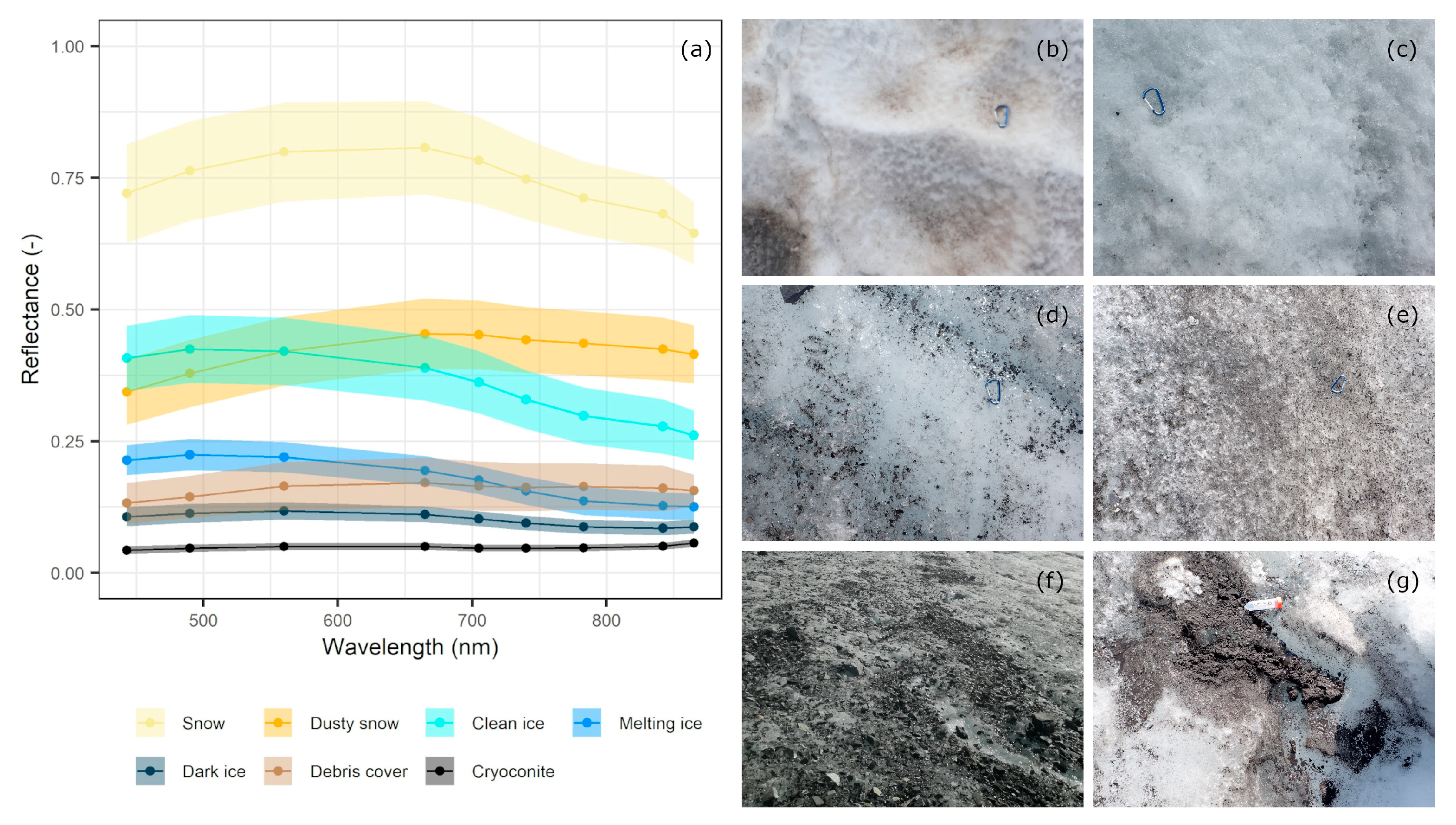
2.3.2. Field Spectroscopy Measurements

Concurrently with the MAIA S2 acquisition, field spectroscopy data were measured with a HandHeld Analytical Spectral Device (ASD) Field Spec (spectral range = 325–1075 nm, spectral sampling interval = 1 nm) on 17 different targets. The hemispherical conical reflectance factor (HCRF) was calculated as the ratio between the radiance reflected by the target and the incident radiance measured from a calibrated 99% Spectralon^® white panel. Each acquisition was the average of 15 spectra. Data were collected from nadir using a 25 deg bare optical fiber at 80 cm from the target surface (corresponding to a footprint diameter of 35 cm).

The measured targets correspond to four reference panels of varying reflectance and thirteen pure surface materials corresponding to the surface types most abundant on the glacier, i.e., clean ice, dark ice, melting ice and cryoconite. The reference panels consist of 50 × 50 cm² panels with a mean reflectance of 93%, 28%, 13% and 5% across bands. They were manufactured using RustOleum^® matte primer and paint on plywood [53]. The coordinates of each target were accurately measured with a dGNSS. Reflectance measurements were taken ± two hours around the multispectral drone overpass under clear-sky conditions. The measurements collected over the reference panels were used to calibrate the MAIA S2 pseudo-reflectance values with the empirical line approach, while those collected over different glacial surface types were used to validate the MAIA S2 reflectance maps.

2.4. High-Resolution Orthoimage and Digital Surface Model Generation

The images collected during the drone surveys with the RGB camera were processed into orthophotos and grid-based DSMs of the glacier and its surroundings using a structure-from-motion (SfM) workflow [54,55] in Agisoft Metashape v. 1.7.2 (Agisoft LLC, St. Petersburg, Russia). A detailed description of the SfM algorithms used in Metashape can be found in Verhoeven [56].

The RGB images were aligned using an image-feature-recognition algorithm similar to Lowe’s [57] scale-invariant feature-transform method, which automatically identifies and matches unique features within the images that are stable with respect to variations in lighting and view perspective across input photographs. Next, a sparse 3D point cloud was produced through an iterative-bundle-adjustment algorithm. The GCPs were then imported together with their dGNSS coordinates, correctly assigned to each image manually, and used to optimize spatial accuracy and improve the geometry of the 3D point cloud. DSM and orthophoto georeferencing was performed with a GCP density of 45 GCP/km² and 1.8 × 10⁻⁸ GCP/GSD (ground-sampling distance) for the RGB survey, compatible with the one recommended by Gindraux et al. [58] for similar drone surveys.

Successively, a multi-view stereo image-matching algorithm was used to increase the density of the point cloud and to convert it by interpolation into DSMs and orthophoto mosaics. DSMs and orthophotos were exported with ground-sampling distances (GSDs) of 0.04 and 0.02 m for the DSMs and orthophotos, respectively.

The horizontal, vertical, and total root mean square error (RMSE) and mean error (ME) with the relative standard deviation (SD) of both GCPs and GVPs were calculated to assess the geometric accuracy of the models.

Two debris banks were identified on the glacier surface, which developed along the glacier’s flow direction, close to the lateral moraine, on the orographic right. Debris thickness was estimated starting from the glacier DSM. First, we masked the areas corresponding to the two debris banks, then we interpolated the elevation values within these areas using the global polynomial interpolation to obtain the actual elevation of the glacial surface without considering the thickness of debris cover. We finally estimated debris thickness by computing the difference between the original and the interpolated elevation values.

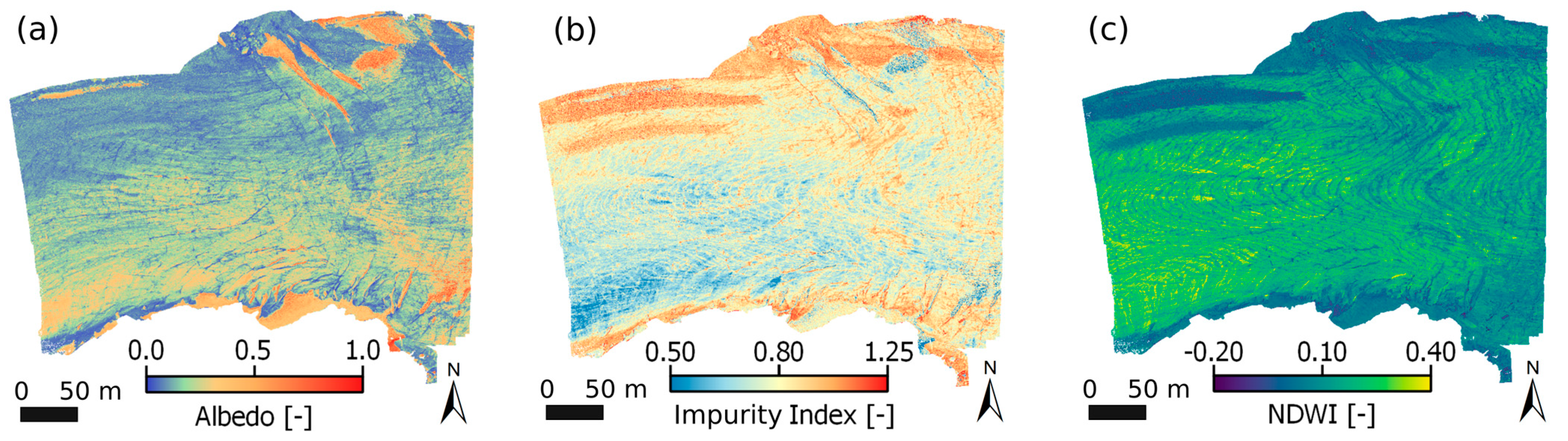
2.5. Multispectral Image Processing and Spectral Index Computation

Image processing, including the geometric and radial calibration, was applied to the raw MAIA S2 imagery using the MultiCam Stitcher Pro software v1.4. A per-pixel vignetting correction was applied to counteract the gradual illumination reduction from the center to the borders of the images. Then, the images collected with the nine sensors of the camera were co-registered based on the photogrammetric method described by Nocerino et al. [50] and Dubbini et al. [51]. The MAIA S2 and ILS (incoming light sensor) logs were matched to that of the drone platform through the GPS time using an R script. This allowed us to assess the MAIA S2 image positioning based on RTK coordinates and yaw, pitch and roll of the drone. Pseudo-reflectance images were then obtained dividing the radiance recorded at pixels of each MAIA S2 band by the incoming radiance measured by the ILS. DN and pseudo-reflectance images were cropped with MultiCam Stitcher Pro software to remove the borders that were not covered by all the 9 sensors of the camera.

DN images and their RTK coordinates were then imported to the SfM processing in Agisoft Metashape v1.7.2 (Agisoft, Russia), and channel 5 was set as the Master channel, being the central one in the MAIA sensor. This means that the software primarily uses that channel to find key points between images and align them. Before the alignment, the camera calibration file was imported to channel 5. These parameters were determined before the campaign with a dedicated flight mission. After the alignment, the workflow was similar to the one described for the RGB image processing, with the only difference regarding the number of GCPs covered by the flights as described in Section 2.3.1. In addition, after DSM generation, we swapped the DN images with the pseudo-reflectance ones, in order to obtain the multispectral orthomosaic. In this context, we set the final orthomosaic resolution to 0.04 m. DSM and orthophoto georeferencing was performed with a GCP density of 91 GCP/km² and 1.46 × 10⁻⁷ GCP/GSD (ground-sampling distance).

Finally, the empirical line method [59] was applied to compute at ground multispectral reflectance. An empirical relationship between the drone pseudo-reflectance and the ground reflectance of the reference panels collected with a HandHeld Analytical Spectral Device (ASD) Field Spec was established for each of the 9 MAIA S2 spectral bands. To perform this, we chose the single images (not the orthomosaic images) where the panels were positioned as much at the center as possible, in order to optimize the calibration coefficient calculation. For this purpose, we resampled the ASD field spectra on the MAIA S2 wavelengths. The linear equation was forced to pass through the origin, following the procedure indicated by Fawcett et al. [53]. The slope coefficient of the line obtained for each multispectral band was applied to the orthomosaic images to obtain the final reflectance map. The performances of the linear fitting models for each band were evaluated in terms of determination coefficient (R²), root mean square error (RMSE), mean absolute deviation (MAD) and relative error (RE%). Starting from the MAIA S2 reflectance maps, several spectral indices developed in cryospheric studies were calculated. Their formulation and the target variables are reported in

Table 3. Spectral indices evaluated in this study. R_λ refers to the reflectance factor at wavelength λ in nm.

Index	Formulation	Target	Reference
Surface albedo	0.726R560 – 0.322$R_{560}^2$ – 0.015R842 – 0.581$R_{842}^2$	Snow and ice brightness	[60]
Impurity index	ln(R560)/ln(R842)	Impurities in snow and ice	[61]
Normalized difference water index (NDWI)	(R560 – R842)/(R560 + R842)	Liquid water on surface ice	[62]

.

Classification of the Multispectral Image

Seven different types of surface covers were observed in the study area during the field surveys and were visually identified on the RGB orthomosaic: snow, clean ice, melting ice, dark ice, cryoconite, dusty snow, and debris cover. Those seven classes of interest were then considered in the preparation of the training dataset for the digital classification of the multispectral orthomosaic, performed in ENVI 5.5 (Harris Geospatial Solutions, Boulder, CO, USA). The support vector machine (SVM) algorithm, a statistical learning theory-based supervised classification method [63,64], was used to classify the images and derive thematic maps with the spatial distribution of the main surfaces. A total of 120 polygons (at least 1000 pixels) per class were manually digitized on the RGB orthomosaic to train the algorithm. These training areas were selected using ancillary information, such as field notes, GPS points and high-resolution RGB orthomosaics. The training design and size were defined following the indications provided by Noi and Kappas [65]. The nine bands of the multispectral images were used as input of the SVM.

Classification accuracy was assessed through confusion matrices [66]. The overall accuracy (OA) of the classification was calculated by dividing the sum of the correctly classified pixels by the total number of pixels taken. The accuracy of the classification was assessed using an independent dataset consisting of a total of 55 polygons of 10 × 10 pixels (40 × 40 cm²). A total of 50 points were randomly placed using a stratified random sampling scheme in QGIS. Each point was then transformed into a 10 × 10 pixels polygon keeping the random point as the polygon center. Pixels inside polygons were manually identified using ancillary information such as field notes and high-resolution RGB orthomosaics. In addition, crevasses were manually digitized by visual inspection using the RGB orthomosaic and the DSM. The reason they were not included in the SVM classification is that they do not represent a surface with a specific spectrum (as the other classes).

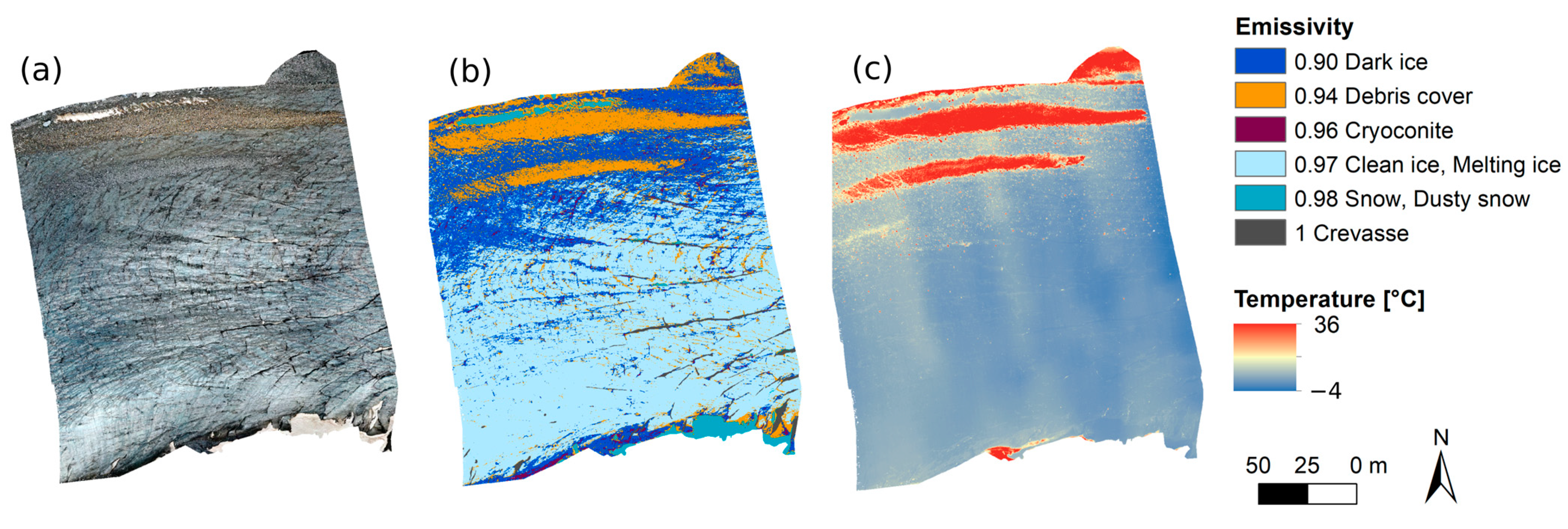
2.6. Thermal Image Processing

The workflow for the generation of the thermal orthophoto is similar to the one described for multispectral image processing. Once the DSM was created, the radiometric jpeg images were replaced with temperature value images, and the temperature orthophoto was created.

The radiance measured by an infrared camera, besides being related to the radiance of the surface of interest, also depends on atmospheric transmissivity τ, radiance reflected from the surroundings and emissivity ε (Equation (1)). Atmospheric transmissivity was estimated assuming an air temperature of 15 °C, relative humidity of 65% and average flight distance of 60 m. The radiance reflected from the surroundings was measured in field using an aluminum reference panel. Emissivity maps were derived from the MAIA S2 classification, assigning to each class an emissivity value derived from previously published studies. The emissivity map was resampled at the TIR orthophotos’ resolution (i.e., 8 cm), using the nearest-neighbor method to calculate the corrected surface temperature. The emissivity value assigned to each class and their relative reference are reported in

Table 4. Emissivity value assigned to each category classified from MAIA S2 images with the relative reference.

Class	Emissivity Value	References
Snow and dusty snow	0.98	[67,68]
Clean ice and melting ice	0.97	[41,67,68]
Dark ice	0.90	[69]
Debris cover	0.94	[41,70]
Cryoconite	0.96	Generic value for organic matter [71]
Crevasses	1

.

Ground surface temperature (T_s) was computed as:

$$T_S=\sqrt[4]{\frac{T_{sensor}{}^4-\left(1-\epsilon \right)\ast {\tau }_{atm}\ast T_{refl}{}^4-\left(1-{\tau }_{atm}\right)\ast T_{atm}{}^4}{\epsilon \ast {\tau }_{atm}}},$$

(1)

where

T_S is the corrected pixel temperature [°K];

ε is the emissivity value assigned to each class;

τ_atm is the atmospheric transmissivity and is set to 0.95 (estimated assuming and air temperature of 15 °C, relative humidity of 65% and average flight distance of 60 m);

T_sensor is the temperature detected by the sensor [°K];

T_refl is the reflected temperature from the surroundings measured in field using an aluminum reference panel and is set to 258.15 °K (−15 °C);

T_atm is the atmospheric temperature and is set to 288.15 °K (15 °C).

Finally, the temperature map was calibrated using a linear empirical calibration developed in laboratory conditions between the XT2 camera and the calibrated FLIR T650sc hand-held thermal-imaging camera using different surfaces at known temperatures.

Unfortunately, only a rather small portion of the glacier was covered by the thermal survey because we experienced problems with camera internal temperature that induced artifacts in different flights.

3. Results

3.1. Drone Imagery Geometric Accuracy

The RMSE, mean error and standard deviation of the GCPs used for model generation and the GVPs used for the assessment of model accuracy are reported in

Table 5. Root mean square error (RMSE), mean error (ME) and standard deviation of error (SD) for red, green and blue (RGB), multispectral (MAIA S2) and thermal infrared (TIR) imagery and both ground control point (GCP) and ground validation point (GVP).

Imagery	GCP	GCP	GCP	GVP	GVP	GVP
	RMSE XY (cm)	RMSE Z (cm)	Total RMSE (cm)	RMSE XY (cm)	RMSE Z (cm)	Total RMSE (cm)
RGB	6.245	6.236	8.826	13.251	10.803	17.097
MAIA S2	0.603	0.039	0.604	1.716	3.001	3.456
TIR	14.6	26.4	30.2	-	-	-
	ME|SDX (cm)	ME|SDY (cm)	ME|SDZ (cm)	ME|SDX (cm)	ME|SDY (cm)	ME|SDZ (cm)
RGB	4.437|1.971	3.249|2.209	5.473|2.989	7.766|6.847	7.407|3.681	10.073|3.906
MAIA S2	0.188|0.105	0.446|0.277	0.028|0.027	1.416|0.899	0.247|0.260	2.808|1.058
TIR	4.6|2.7	14.4|7.0	28.0|12.0	-	-	-

.

The total RMSE computed on the GVPs was 17 cm for the RGB models and about 3.5 cm for the multispectral images. The mean error over the whole study area was lower than 5 cm for the GCP and lower than 10 cm for the GVP. For the multispectral images, the mean error was always lower than 2 cm, and in many cases, it was lower than 1 cm. The higher error of TIR orthophotos can be ascribed to the lower resolution of thermal images and the low spatial variability of surface temperature on the glacier tongue.

3.2. Calibration and Validation of Drone Derived Reflectance

An empirical relationship between MAIA S2 pseudo-reflectance and ground-measured HCRF reflectance over the four reference panels was established for each of the nine MAIA S2 spectral bands. The pseudo-reflectance maps obtained after the correction for the irradiance measured using the ILS showed very good spectral shapes and good agreement with the spectral measurements collected on the ground with the ASD spectrometer (R²: 0.97–0.98). The linear equation with the intercept set to zero obtained for each multispectral band was then applied to produce the final reflectance of the multispectral images. The slope of the linear equation and the fitting statistics for each band are reported in

Table 6. Slope and fitting statistics (R², RMSE, MAD and RE%) of the linear equation obtained between MAIA S2 and ground-measured reflectance over the four reference panels for each of the 9 MAIA S2 spectral bands.

	B1 (443)	B2 (490)	B3 (560)	B4 (665)	B5 (705)	B6 (740)	B7 (783)	B8 (842)	B9 (865)
Slope	3.08	3.16	2.91	2.59	2.86	2.57	2.33	2.67	2.90
R2	0.98	0.98	0.98	0.98	0.98	0.98	0.97	0.97	0.97
RMSE	0.025	0.027	0.027	0.030	0.030	0.032	0.037	0.040	0.045
MAD	0.019	0.021	0.022	0.026	0.025	0.028	0.032	0.035	0.040
RE (%)	12.26	12.73	13.48	15.84	15.97	18.33	22.19	25.10	28.12

.

MAIA S2 reflectance was then validated against ASD HCRF measured over 13 independent homogeneous targets. The fitting statistics of the linear equations with the intercept set to zero obtained for each multispectral band are reported in

Table 7. Fitting statistics (R², RMSE, MAD and RE%) of the linear equation obtained between MAIA S2 and ground reflectance measured over 13 independent homogeneous targets.

	B1 (443)	B2 (490)	B3 (560)	B4 (665)	B5 (705)	B6 (740)	B7 (783)	B8 (842)	B9 (865)
R2	0.914	0.909	0.907	0.884	0.862	0.827	0.767	0.722	0.699
RMSE	0.027	0.029	0.030	0.033	0.033	0.035	0.041	0.044	0.047
MAD	0.021	0.023	0.024	0.029	0.029	0.031	0.036	0.039	0.041
RE (%)	13.878	13.832	14.338	17.746	18.141	20.613	25.278	28.497	30.506

.

Overall, errors per band were in the 2–4% reflectance range, which equals 13–30% relative error.

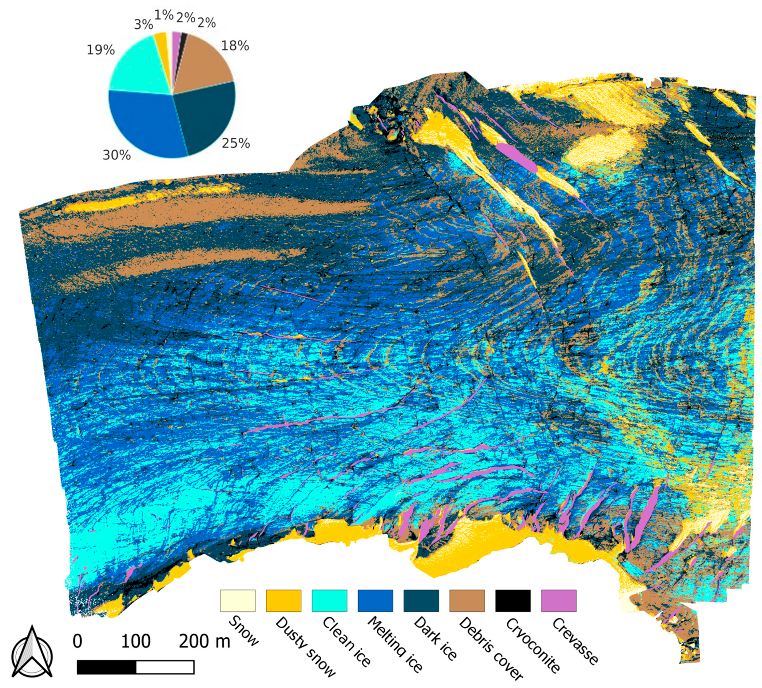
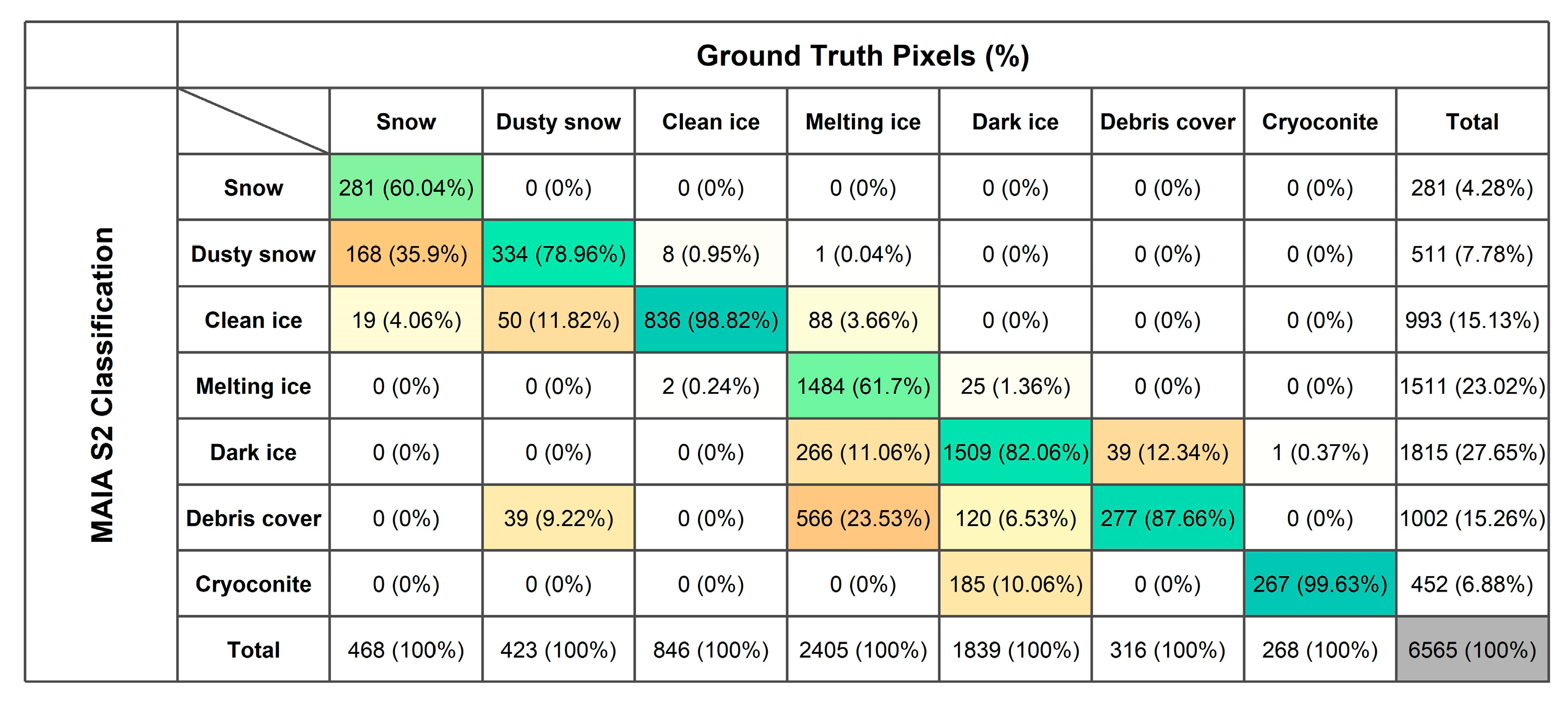
3.3. Classification of the Multispectral Orthomosaics and Accuracy Evaluation

Mean reflectance and standard deviation of the training classes used for the classification procedure are shown in Figure 3.

Clean snow shows an average reflectance in the visible and near-infrared wavelengths higher than that of the other classes (up to 0.8 in the green–red bands). Dusty snow shows lower reflectance on the entire spectrum, with reflectance values of about 0.45 at 650–700 nm. Particularly, the presence of impurities in snow causes a decrease in the reflectance at wavelengths in the blue and green [72]. The reflectance curves for clean ice exhibit the typical shape frequently found in the literature [14], with the highest reflectance values (up to 0.58) in the green region and declining values for longer wavelengths. The spectral reflectance curves of melting ice and dark ice surfaces have a shape similar to the one of clean ice, but they are greatly reduced in amplitude, with reflectance values typically not exceeding 0.25 and 0.15, respectively. Reflectance values of debris-covered surfaces have almost stable reflectance across the investigated spectral range and similar average magnitudes to those for melting ice. Cryoconite shows the darkest spectral profiles, and their reflectance remains at uniformly low values below 0.1 at all measured bands [7,73].

The thematic map obtained with the SVM algorithm is shown in Figure 4.

Different surface types present on the glacier were classified with an overall accuracy of 76% and a kappa coefficient [74] of 0.70. The confusion matrix obtained from crossing the ground truth data with the results of the classification is shown in Figure 5.

Snow, dusty snow, bright ice, melting ice, dark ice, debris cover, cryoconite and crevasse were classified. Clean ice, dark ice, dusty snow, debris cover and cryoconite were classified with very high accuracies of about 80–99%. A moderate accuracy of about 60% was found for snow and melting ice. The largest confusion was found between snow and dusty snow (36%), melting ice and debris cover (23%), melting ice and dark ice (11%) and dusty snow and clean ice (11.8%). The greatest portion of the investigated area consisted of different ice types, namely clean ice (19%), dark ice (24%) and melting ice (30%). The ablation area also showed extensive coverage of debris (17%) and cryoconite (2%). Snow (1%) and dusty snow (3%) were present on the margins of the Zebrù glacier tongue.

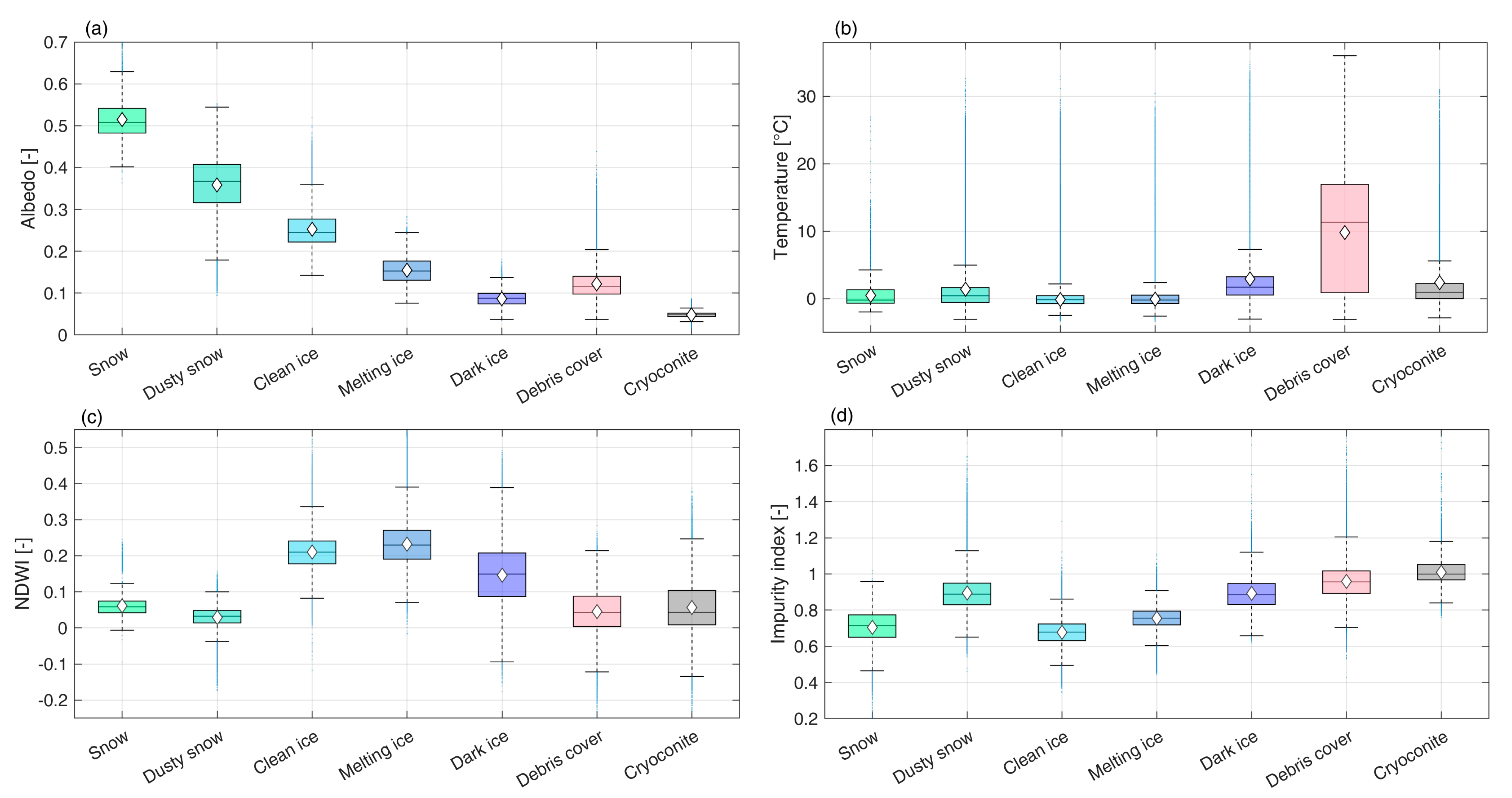
3.4. Relationship between Surface Types, Temperature and Spectral Indices

The products derived from the MAIA S2 data and the temperature maps are shown in Figure 6 and Figure 7, respectively. The albedo and impurity index maps (Figure 6a,b) show a north–south gradient over the glacier. The north-facing side of the glacier is impacted by frequent depositions of fine and coarse debris from the south-facing slope of Monte Zebrù. The process progressively darkened the surface of the glacier, which features lower albedo and higher impurity index values in this area. Here, two thick debris deposits were mapped (Figure 4). They are likely related to past deposition of debris on the glacier that was transported and redistributed by the glacier flow, and they now display an elongated shape following the glacier south–west movement.

High NDWI values identify the areas of the glacier where we can find surface liquid water flowing as bédière on the ice. This can further influence the radiative balance of glacier ice by absorbing more radiation and inducing further surface melting.

In Figure 7, we present results for the central part of the ablation area of the Zebrù glacier. We show the RGB representation of the glacier portion covered with the thermal survey, the emissivity map, and the derived surface temperature map. Interestingly, this area displays all different surface classes present on the glacier, and this allowed us to compare the variability of spectral indices and glacier surface temperature according to surface type (Figure 8).

Analysis of the thermal image showed that the glacier surface is characterized by a wide range of temperatures, from −4 to 36 °C (Figure 7c).

Among the different surface types identified on the glacier (Figure 7b and Figure 8b), the lowest temperatures were found on clean and melting ice and snow, with the average temperature variable between −0.1 (clean ice) and 0.5 °C (snow). Dusty snow, dark ice and cryoconite are warmer than ice and snow with an average temperature between 1.4 (dusty snow) and 3 °C (dark ice). This is due to the presence of impurities that lower the albedo, so there is a higher absorption of radiation that results in higher temperature values. Debris cover, occupying 17% of the surface, showed the highest temperatures (i.e., average temperatures of 9.8 °C).

Looking at the albedo values (Figure 8a), snow and dusty snow had the highest values. Then, a negative variation was observed in clean ice (average value of 0.25 ± 0.04), melting ice (0.15 ± 0.03), and finally, dark ice (0.09 ± 0.01). This trend is explained by the fact that melting ice has a film of water on the surface, which lowers its reflectivity, while dark ice has very low albedo values, which favors absorption rather than reflection. The NDWI shows higher values in the ice classes than in the other identified classes (Figure 8c). As expected, the impurity index assumes higher values in the correspondence of the classes characterized by the presence of impurities (i.e., dusty snow, dark ice, debris cover and cryoconite) (Figure 8d).

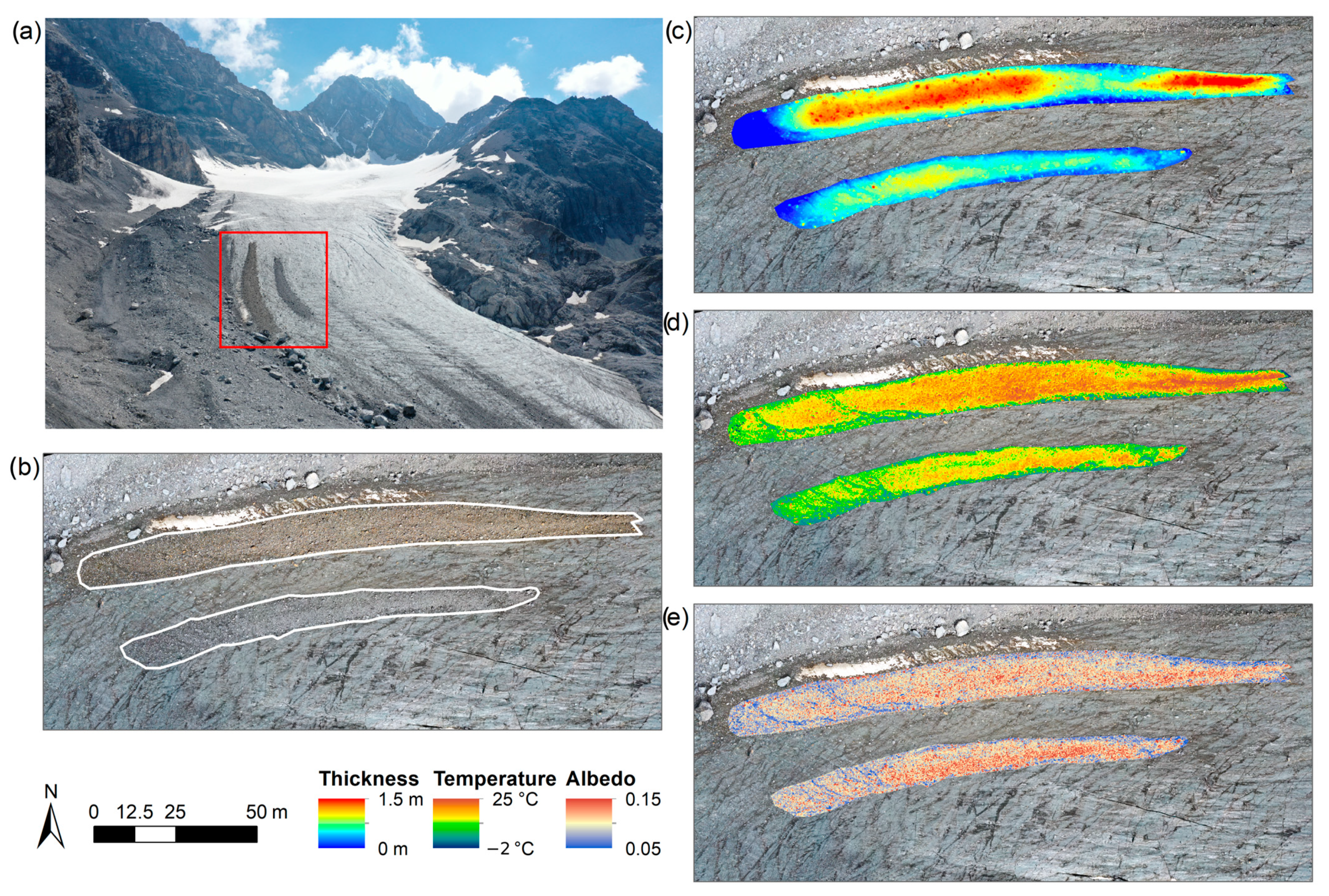
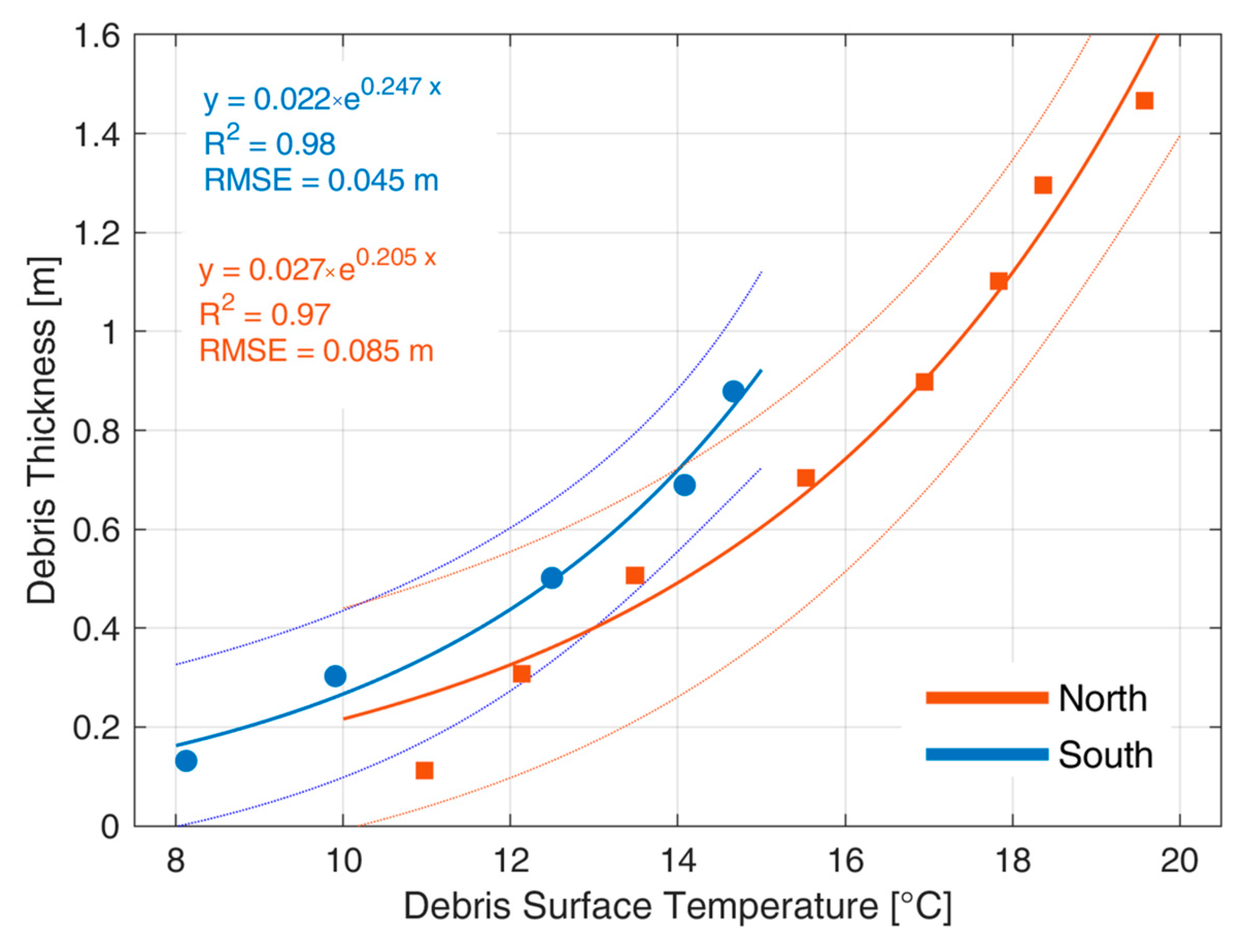
3.5. Relationship between Surface Temperature and Debris Thickness

In Figure 9, we present a focus on the two debris-cover structures that we found on the Zebrù glacier. We refer to these structures as debris cover located on the north and south of the glacier ablation area (Figure 9a,b). For these two structures, we show the derived thickness (Figure 9c), surface temperature (Figure 9d) and albedo (Figure 9e). The debris cover located to the north showed a higher thickness and higher surface temperature with respect to the one located to the south. Conversely, albedo values are slightly higher in the debris cover to the south. From Figure 9b, we can observe that the rock material that constitutes the debris has a different mineralogy in the two structures. In particular, the north one is redder, and the south one shows a grey color. This particular characteristic motivated us to analyze more in detail the dependence of the debris cover on surface temperature.

Comparing the debris thickness aggregated in thickness classes of 0.2 m each with surface temperature, we obtained an empirical exponential relation between the measured debris thickness and debris surface temperatures as observed by Tarca and Guglielmin [43] (Figure 10). Two different curves were used for the north and south debris-cover area because they are composed of a different lithology, and this affects the surface temperatures. The southern bank has a higher temperature than the northern bank for the same thickness.

4. Discussion

This paper demonstrates that drone surveys can be successfully used to map surface features of an Alpine glacier and characterize its surface temperature. High-resolution mapping of different snow and ice types and the occurrence of light-absorbing impurities is key for a better understanding of glacier’s energy budget and melt rates.

4.1. Uncertainty Analysis and Sources of Errors

To achieve accurate reflectance maps and maintain comparability across different drone surveys, appropriate radiometric and atmospheric corrections need to be applied. For this reason, the development of a reliable method for a multispectral drone imaging campaign is important for both research and practical applications. This aspect is particularly important in view of the growing number of lightweight multispectral sensors and increasing amounts of imagery acquired by different sensors. In this study, pseudo-reflectance maps are first obtained by means of an irradiance sensor levelled and positioned on the ground to increase measurement stability. As already discussed in previous studies, the irradiance sensor needs to be stabilized using an onboard gimbal or by being installed on the ground to obtain accurate absolute irradiance measurement [75,76]. However, spatial differences in incident irradiance due to low, moving clouds could affect the pseudo-reflectance maps if the irradiance measurements are collected on the ground at some distance from the drone [77]. Thus, the method used in this study is recommended only when the flights are performed under spatially stable illumination conditions (e.g., clear-sky conditions, high cirrus clouds). Pseudo-reflectance maps were then further refined through the empirical line approach, accounting for atmospheric effects that might become significant when flying at high altitudes, followed by independent validation of the HCRF maps. The results of the HCRF validation confirmed the validity of the proposed workflow, leading to accurate HCRF maps with MAD lower than 0.04. The differences between field and drone spectra were comparable to those of other studies using similar sensors [53,78,79]. These studies mainly focused on vegetation analyses, while very few examples of multispectral-drone-based studies for cryospheric research can be found in the literature [37]. Lower accuracy was achieved in the near-infrared bands, where the MAIA sensor tends to underestimate high reflectance values. Differences between field and drone spectra can be related to a difference in size of ASD field of view and MAIA pixel size. We selected targets that were considered homogenous within the field spectrometer’s field of view projection on the ground. However, small-scale spatial variations are always present in natural surfaces and can be considered a source of uncertainty. The heterogeneous nature of the glacial surface can be appreciated in both Figure 2c and Figure 3b–g. A detailed description of the possible sources of error and their impact on sensor validation can also be found in Naethe et al. [77]. Recently, besides multispectral cameras, the use of TIR cameras on drones has been promoted by the availability of miniaturized lightweight thermal sensors that can be carried by several commercial drone platforms. However, obtaining absolute temperatures of the glacier surface using drone-based thermal imaging is not trivial [41,80,81]. First, the camera needs to be warmed up for a certain amount of time before being able to collect stable radiometric temperature values. Second, as most of the available commercial drones mount uncooled microbolometers, a series of calibrated resistance temperature detectors can be used to calibrate the camera in laboratory conditions and to derive the calibration equations [82]. Lastly, an in situ thermal reference may be placed on the surveyed areas to validate the retrieved surface temperature.

Our XT2 thermal camera needed about 20 min before being stabilized. Nevertheless, the transition areas between different flights can be seen in the temperature maps (Figure 7c). These are due to imperfect stabilization of the camera that may introduce additional uncertainties to the absolute glacier surface temperatures. However, those differences fall within the temperature accuracy of the camera, which is equal to ±2.0 °C [40].

Then, the thermal signal measured by the camera is a combination of the radiometric temperature of the surface of interest, the atmospheric transmissivity τ, the radiance reflected from the surroundings and the emissivity ε. Previous works, such as that conducted by Aubry-Wake et al. [83] and Kraaijenbrink et al. [41], assigned different emissivity values to broad classes identified using RGB images. Here, we exploited the high-spatial-resolution multispectral classification to assign to each temperature pixel the appropriate emissivity value.

Since in our study the temperatures from the thermal image were not compared to in situ values, they could suffer from possible bias when examining absolute values. However, the retrieved temperature values are in line with those reported in similar studies [20,40,83] and assume a value close to 0 °C over melting ice surfaces. This can be considered a good indicator of the reliability of the obtained maps in the absence of any in situ measurements [44].

In addition, we should consider that the processing of thermal data with SfM can be problematic due to the consequence of the lower resolution of thermal images compared with RGB. Small features, especially in areas with homogeneous surface temperature (e.g., glacier), are less or not visible in the thermal imagery [84].

4.2. Mapping of Glacier Surface Types

Using reliable multispectral images as input of the SVM algorithm, we were able to distinguish different surface types present on the ablation area of the investigated glacier, which is consistent with studies in other research fields (e.g., [7,85]). The glacier surface is characterized by a large heterogeneity of surface types. This pattern is likely created by the melting itself that redistributes surface debris and organic material, creating a preferential flow of liquid water on the glacier. At the Zebrù glacier, we did not find evidence of algal communities that are able to selectively absorb solar radiation in the visible wavelengths [86]. The high spatial resolution of the drone survey, coupled with the multispectral characteristics of the MAIA S2 sensor, enabled a clear distinction between snow, dusty snow, clean ice, melting ice, dark ice, debris cover, cryoconite and crevasses. The largest confusion was found between snow and dusty snow (36%) and between melting ice and dark ice (11%). This can be explained by the difficulty to distinguish between them even in the field as the transition from one class to the other is smooth in nature. During the summer season, surface snow is often darkened by the accumulation of atmospheric impurities deposited during the winter and spring season. Thus, the two classes “snow” and “dusty snow” show very high similarity. Confusion was also observed between dusty snow and clean ice; however, these classes occur on a very limited number of pixels within the surveyed areas. The glacier surface is therefore a heterogeneous mixture of various materials, which is hard to capture with direct measurements. The drone-based classifications could provide valuable high-spatial-resolution information regarding the distribution of snow and ice types and the presence of supraglacial material in the ablation zone of the glacier, allowing the investigation of their impact on glacier albedo and performance of the energy and mass balance of glaciers. Only few studies have investigated the spatial and temporal variability in the spectral properties and albedo of the bare-ice surface types that characterize the ablation zone. So far, they have often been considered temporal and spatial constants in surface melt models. However, taking into account the growing dominance of bare-ice areas with respect to the overall glacier area, the sensitivity of the glacier mass and energy balance to variations in ice-reflectance properties has become of increasing interest in recent years [14]. Average albedo values of bare ice at the Zebrù glaciers were found to be lower than 0.3. These are remarkably low values for a non-debris-covered glacier. The albedo map could be assimilated by the glacier mass-balance model to evaluate at unprecedented scale the impact of surface darkening on ice melting [87]. Furthermore, spectral indices derived from multispectral data may help in interpreting the spatial pattern of the surface mass balance of glaciers by identifying surface features (e.g., distributed cryoconite, sparse debris, ogives, algae, etc.) that may contribute to surface lowering during the summer season [7,88].

4.3. Opportunities of Drone-Derived Thermal Data for Glacier Monitoring

Optical and thermal data have been often used to estimate near-surface snow characteristics, for example, surface albedo, grain size, light-absorbing impurities, snow surface temperature and spectral emissivity [83,89,90,91,92]. Recently, Colombo et al. [93] showed that coupled optical and thermal data can be used to estimate snowpack density through the apparent thermal inertia.

Here, thermal infrared images were used to analyze glacier thermal variations at very high spatial resolution, enabling the investigation of the effect of surface cover type on the glacier’s temperature. In agreement with the few other studies using drone and ground-based TIR imaging to map glacial surface temperatures [83], snow and ice showed the coldest temperatures, while debris showed the highest ones. At the time of flight, the debris temperature reached up to 36 °C, a value higher than air temperature, which was 15 °C.

An important application of high-resolution thermal imagery shown in this study is the estimation of debris-cover thickness, as the presence of debris on a glacier causes an increase in glacier’s mean surface temperature. Between the two debris-covered structures, the northern one is warmer than the southern one. This can be explained by the higher thickness of the former and by the different lithological composition of pebbles in the two areas. Indeed, the two areas of debris cover are composed of different lithologies: black limestones characterize the northern sediments, while light-grey dolomites those located to the south, and consequently, they exhibit different surface temperatures. The different petrographic nature of these two sedimentary deposits is linked to the geology of the glacial basin. The mountains surrounding the Zebrù glacier (Figure 1) consist of two distinct superimposed formations: the Dolomia Principale, with well-bedded grey dolostones, and the Calcare di Quattervals, composed of black, laminated organic rich shales, dark grey marls and limestones. The northern area has, in fact, a slightly lower temperature than the south one for the same thickness. The surface temperature is affected by the rock lithology, with the different rock lithologies characterized by different radiative and thermal properties (e.g., emissivity, thermal conductivity, specific heat).

The high-resolution thermal imagery has potential applications in the estimation of debris-cover thickness, an important variable in the surface energy balance of debris-covered glaciers. This would improve our understanding of small-scale glacio-hydrological surface processes on debris-covered glaciers.

So far, the estimation of debris thickness from high-resolution thermal data was shown in a limited number of studies [43,44,94]. The creation of high-resolution and spatially distributed debris thicknesses maps allows one to overcome the issue of the mixed pixel effect, often occurring when using satellite data to estimate surface temperature distribution due to their low spatial resolution (ranging from 60 to 100 m pixel size). A previous study showed that using mean debris thickness values in surface mass-balance models will presumably cause melt to be underestimated [95].

A limitation of our study is the scarcity of ground measurements of debris thickness for validation, which may result in uncertainty in the estimation of debris thicknesses from thermal drone data. Further studies linking drone thermal data and in situ debris thickness measurements within surveyed areas would yield better establishment of the accuracy of these debris thicknesses maps.

5. Conclusions

In this paper, we demonstrated that the integration of multispectral and thermal drone imaging can support glaciological studies. We accurately validated reflectance data observed from the multispectral camera with field spectroscopy data (MAD < 0.04 for HCRF), and we applied an SVM algorithm to the multispectral data for the classification of different surface types on an Alpine glacier (overall accuracy = 76% and kappa coefficient = 0.7). We identified a very high heterogeneity of surface types dominated by melting ice (30% of the investigated area), dark ice (24%), clean ice (19%) and debris cover (17%). An emissivity thematic map was then used to estimate the surface temperature of the glacier. These data were combined with a high-resolution DSM of the glacier to evaluate the dependence between surface temperature and debris thickness. We found out that this dependence is influenced by the petrology of debris cover, suggesting the importance of lithology when considering the role of debris over glaciers.

References

1. Paul, F.; Rastner, P.; Azzoni, R.S.; Diolaiuti, G.; Fugazza, D.; Le Bris, R.; Nemec, J.; Rabatel, A.; Ramusovic, M.; Schwaizer, G.; et al. Glacier Shrinkage in the Alps Continues Unabated as Revealed by a New Glacier Inventory from Sentinel-2. Earth Syst. Sci. Data 2020, 12, 1805–1821. [Google Scholar] [CrossRef]
2. Zemp, M.; Frey, H.; Gärtner-Roer, I.; Nussbaumer, S.U.; Hoelzle, M.; Paul, F.; Haeberli, W.; Denzinger, F.; Ahlstrøm, A.P.; Anderson, B.; et al. Historically Unprecedented Global Glacier Decline in the Early 21st Century. J. Glaciol. 2015, 61, 745–762. [Google Scholar] [CrossRef] [Green Version]
3. Barandun, M.; Bravo, C.; Grobety, B.; Jenk, T.; Fang, L.; Naegeli, K.; Rivera, A.; Cisternas, S.; Münster, T.; Schwikowski, M. Anthropogenic Influence on Surface Changes at the Olivares Glaciers; Central Chile. Sci. Total Environ. 2022, 833, 155068. [Google Scholar] [CrossRef] [PubMed]
4. Di Mauro, B.; Fugazza, D. Pan-Alpine Glacier Phenology Reveals Lowering Albedo and Increase in Ablation Season Length. Remote Sens. Environ. 2022, 279, 113119. [Google Scholar] [CrossRef]
5. Nakawo, M.; Young, G.J. Estimate of Glacier Ablation under a Debris Layer from Surface Temperature and Meteorological Variables. J. Glaciol. 1982, 28, 29–34. [Google Scholar] [CrossRef] [Green Version]
6. Mihalcea, C.; Mayer, C.; Diolaiuti, G.; Lambrecht, A.; Smiraglia, C.; Tartari, G. Ice Ablation and Meteorological Conditions on the Debris-Covered Area of Baltoro Glacier, Karakoram, Pakistan. Ann. Glaciol. 2006, 43, 292–300. [Google Scholar] [CrossRef] [Green Version]
7. Di Mauro, B.; Baccolo, G.; Garzonio, R.; Giardino, C.; Massabò, D.; Piazzalunga, A.; Rossini, M.; Colombo, R. Impact of Impurities and Cryoconite on the Optical Properties of the Morteratsch Glacier (Swiss Alps). Cryosphere 2017, 11, 2393–2409. [Google Scholar] [CrossRef] [Green Version]
8. Rozwalak, P.; Podkowa, P.; Buda, J.; Niedzielski, P.; Kawecki, S.; Ambrosini, R.; Azzoni, R.S.; Baccolo, G.; Ceballos, J.L.; Cook, J.; et al. Cryoconite—From Minerals and Organic Matter to Bioengineered Sediments on Glacier’s Surfaces. Sci. Total Environ. 2022, 807, 150874. [Google Scholar] [CrossRef]
9. Paul, F.; Kääb, A.; Haeberli, W. Recent Glacier Changes in the Alps Observed by Satellite: Consequences for Future Monitoring Strategies. Glob. Planet. Chang. 2007, 56, 111–122. [Google Scholar] [CrossRef]
10. Naegeli, K.; Huss, M.; Hoelzle, M. Change Detection of Bare-Ice Albedo in the Swiss Alps. Cryosphere 2019, 13, 397–412. [Google Scholar] [CrossRef] [Green Version]
11. Arendt, A. Approaches to Modelling the Surface Albedo of a High Arctic Glacier. Geogr. Ann. Ser. A Phys. Geogr. 1999, 81, 477–487. [Google Scholar] [CrossRef]
12. Pope, E.L.; Willis, I.C.; Pope, A.; Miles, E.S.; Arnold, N.S.; Rees, W.G. Contrasting Snow and Ice Albedos Derived from MODIS, Landsat ETM+ and Airborne Data from Langjökull, Iceland. Remote Sens. Environ. 2016, 175, 183–195. [Google Scholar] [CrossRef] [Green Version]
13. Wehrlé, A.; Box, J.E.; Niwano, M.; Anesio, A.M.; Fausto, R.S. Greenland Bare-Ice Albedo from PROMICE Automatic Weather Station Measurements and Sentinel-3 Satellite Observations. GEUS Bull. 2021, 47, 1–9. [Google Scholar] [CrossRef]
14. Hartl, L.; Felbauer, L.; Schwaizer, G.; Fischer, A. Small-Scale Spatial Variability in Bare-Ice Reflectance at Jamtalferner, Austria. Cryosphere 2020, 14, 4063–4081. [Google Scholar] [CrossRef]
15. Naegeli, K.; Huss, M. Sensitivity of Mountain Glacier Mass Balance to Changes in Bare-Ice Albedo. Ann. Glaciol. 2017, 58, 119–129. [Google Scholar] [CrossRef] [Green Version]
16. Naegeli, K.; Damm, A.; Huss, M.; Schaepman, M.; Hoelzle, M. Imaging Spectroscopy to Assess the Composition of Ice Surface Materials and Their Impact on Glacier Mass Balance. Remote Sens. Environ. 2015, 168, 388–402. [Google Scholar] [CrossRef]
17. Klok, E.J.; Greuell, W.; Oerlemans, J. Temporal and Spatial Variation of the Surface Albedo of Morteratschgletscher, Switzerland, as Derived from 12 Landsat Images. J. Glaciol. 2004, 49, 491–502. [Google Scholar] [CrossRef] [Green Version]
18. Arnold, N.S.; Willis, I.C.; Sharp, M.J.; Richards, K.S.; Lawson, W.J. A Distributed Surface Energy-Balance Model for a Small Valley Glacier. I. Development and Testing for Haut Glacier d’ Arolla, Valais, Switzerland. J. Glaciol. 1996, 42, 77–89. [Google Scholar] [CrossRef] [Green Version]
19. Klok, E.J.; Oerlemans, J. Model Study of the Spatial Distribution of the Energy and Mass Balance of Morteratschgletscher, Switzerland. J. Glaciol. 2002, 48, 505–518. [Google Scholar] [CrossRef] [Green Version]
20. Tarca, G.; Guglielmin, M. Evolution of the Sparse Debris Cover during the Ablation Season at Two Small Alpine Glaciers (Gran Zebrù and Sforzellina, Ortles-Cevedale Group). Geomorphology 2022, 409, 108268. [Google Scholar] [CrossRef]
21. Bozhinskiy, A.N.; Krass, M.S.; Popovnin, V.V. Role of Debris Cover in the Thermal Physics of Glaciers. J. Glaciol. 1986, 32, 255–266. [Google Scholar] [CrossRef] [Green Version]
22. Owen, L.A.; Derbyshire, E.; Scott, C.H. Contemporary sediment production and transfer in high-altitude glaciers. Sediment. Geol. 2003, 155, 13–36. [Google Scholar] [CrossRef] [Green Version]
23. Reznichenko, N.; Davies, T.; Shulmeister, J.; McSaveney, M. Effects of Debris on Ice-Surface Melting Rates: An Experimental Study. J. Glaciol. 2010, 56, 384–394. [Google Scholar] [CrossRef] [Green Version]
24. Rounce, D.R.; Hock, R.; McNabb, R.W.; Millan, R.; Sommer, C.; Braun, M.H.; Malz, P.; Maussion, F.; Mouginot, J.; Seehaus, T.C.; et al. Distributed Global Debris Thickness Estimates Reveal Debris Significantly Impacts Glacier Mass Balance. Geophys. Res. Lett. 2021, 48, e2020GL091311. [Google Scholar] [CrossRef]
25. Fugazza, D.; Senese, A.; Azzoni, R.S.; Maugeri, M.; Maragno, D.; Diolaiuti, G.A. New Evidence of Glacier Darkening in the Ortles-Cevedale Group from Landsat Observations. Glob. Planet. Chang. 2019, 178, 35–45. [Google Scholar] [CrossRef]
26. Konig, M.; Winther, J.; Isaksson, E. From and Glacier Satellite. Rev. Geophys. 2001, 29, 1–27. [Google Scholar] [CrossRef]
27. Gaffey, C.; Bhardwaj, A. Applications of Unmanned Aerial Vehicles in Cryosphere: Latest Advances and Prospects. Remote Sens. 2020, 12, 948. [Google Scholar] [CrossRef] [Green Version]
28. Bhardwaj, A.; Sam, L.; Akanksha; Martín-Torres, F.J.; Kumar, R. UAVs as Remote Sensing Platform in Glaciology: Present Applications and Future Prospects. Remote Sens. Environ. 2016, 175, 196–204. [Google Scholar] [CrossRef]
29. Immerzeel, W.W.; Kraaijenbrink, P.D.A.; Shea, J.M.; Shrestha, A.B.; Pellicciotti, F.; Bierkens, M.F.P.; De Jong, S.M. High-Resolution Monitoring of Himalayan Glacier Dynamics Using Unmanned Aerial Vehicles. Remote Sens. Environ. 2014, 150, 93–103. [Google Scholar] [CrossRef]
30. Jawak, S.D.; Wankhede, S.F.; Luis, A.J.; Balakrishna, K. Multispectral Characteristics of Glacier Surface Facies (Chandra-Bhaga Basin, Himalaya, and Ny-Ålesund, Svalbard) through Investigations of Pixel and Object-Based Mapping Using Variable Processing Routines. Remote Sens. 2022, 14, 6311. [Google Scholar] [CrossRef]
31. Ryan, J.C.; Hubbard, A.; Stibal, M.; Irvine-Fynn, T.D.; Cook, J.; Smith, L.C.; Cameron, K.; Box, J. Dark Zone of the Greenland Ice Sheet Controlled by Distributed Biologically-Active Impurities. Nat. Commun. 2018, 9, 1065. [Google Scholar] [CrossRef] [PubMed] [Green Version]
32. Bearzot, F.; Garzonio, R.; Di Mauro, B.; Colombo, R.; Cremonese, E.; Crosta, G.B.; Delaloye, R.; Hauck, C.; Morra Di Cella, U.; Pogliotti, P.; et al. Kinematics of an Alpine Rock Glacier from Multi-Temporal UAV Surveys and GNSS Data. Geomorphology 2022, 402, 108116. [Google Scholar] [CrossRef]
33. Bearzot, F.; Garzonio, R.; Colombo, R.; Crosta, G.B.; Di Mauro, B.; Fioletti, M.; Di Cella, U.M.; Rossini, M. Flow Velocity Variations and Surface Change of the Destabilised Plator Rock Glacier (Central Italian Alps) from Aerial Surveys. Remote Sens. 2022, 14, 635. [Google Scholar] [CrossRef]
34. Cook, K.L. An Evaluation of the Effectiveness of Low-Cost UAVs and Structure from Motion for Geomorphic Change Detection. Geomorphology 2017, 278, 195–208. [Google Scholar] [CrossRef]
35. Benoit, L.; Gourdon, A.; Vallat, R.; Irarrazaval, I.; Gravey, M.; Lehmann, B.; Prasicek, G.; Gräff, D.; Herman, F.; Mariethoz, G. A High-Resolution Image Time Series of the Gorner Glacier—Swiss Alps—Derived from Repeated Unmanned Aerial Vehicle Surveys. Earth Syst. Sci. Data 2019, 11, 579–588. [Google Scholar] [CrossRef] [Green Version]
36. Rossini, M.; Di Mauro, B.; Garzonio, R.; Baccolo, G.; Cavallini, G.; Mattavelli, M.; De Amicis, M.; Colombo, R. Rapid Melting Dynamics of an Alpine Glacier with Repeated UAV Photogrammetry. Geomorphology 2018, 304, 159–172. [Google Scholar] [CrossRef]
37. Tedstone, A.J.; Cook, J.M.; Williamson, C.J.; Hofer, S.; McCutcheon, J.; Irvine-Fynn, T.; Gribbin, T.; Tranter, M. Algal Growth and Weathering Crust State Drive Variability in Western Greenland Ice Sheet Ice Albedo. Cryosphere 2020, 14, 521–538. [Google Scholar] [CrossRef] [Green Version]
38. Cook, J.M.; Tedstone, A.J.; Williamson, C.; McCutcheon, J.; Hodson, A.J.; Dayal, A.; Skiles, M.; Hofer, S.; Bryant, R.; McAree, O.; et al. Glacier Algae Accelerate Melt Rates on the South-Western Greenland Ice Sheet. Cryosphere 2020, 14, 309–330. [Google Scholar] [CrossRef] [Green Version]
39. Healy, S.M.; Khan, A.L. Albedo Change from Snow Algae Blooms Can Contribute Substantially to Snow Melt in the North Cascades, USA. Commun. Earth Environ. 2023, 4, 142. [Google Scholar] [CrossRef]
40. Forte, E.; Santin, I.; Ponti, S.; Colucci, R.R.; Gutgesell, P.; Guglielmin, M. New Insights in Glaciers Characterization by Differential Diagnosis Integrating GPR and Remote Sensing Techniques: A Case Study for the Eastern Gran Zebrù Glacier (Central Alps). Remote Sens. Environ. 2021, 267, 112715. [Google Scholar] [CrossRef]
41. Kraaijenbrink, P.D.A.; Shea, J.M.; Litt, M.; Steiner, J.F.; Treichler, D.; Koch, I.; Immerzeel, W.W. Mapping Surface Temperatures on a Debris-Covered Glacier with an Unmanned Aerial Vehicle. Front. Earth Sci. 2018, 6, 64. [Google Scholar] [CrossRef] [Green Version]
42. Herreid, S. What Can Thermal Imagery Tell Us About Glacier Melt Below Rock Debris? Front. Earth Sci. 2021, 9, 681059. [Google Scholar] [CrossRef]
43. Tarca, G.; Guglielmin, M. Using Ground-Based Thermography to Analyse Surface Temperature Distribution and Estimate Debris Thickness on Gran Zebrù Glacier (Ortles-Cevedale, Italy). Cold Reg. Sci. Technol. 2022, 196, 103487. [Google Scholar] [CrossRef]
44. Gök, D.T.; Scherler, D.; Anderson, L.S. High-resolution debris-cover mapping using UAV-derived thermal imagery: Limits and opportunities. Cryosphere 2023, 17, 1165–1184. [Google Scholar] [CrossRef]
45. Aubry-Wake, C.; Lamontagne-Hallé, P.; Baraër, M.; McKenzie, J.M.; Pomeroy, J.W. Using Ground-Based Thermal Imagery to Estimate Debris Thickness over Glacial Ice: Fieldwork Considerations to Improve the Effectiveness. J. Glaciol. 2023, 69, 353–369. [Google Scholar] [CrossRef]
46. Mihalcea, C.; Mayer, C.; Diolaiuti, G.; D’Agata, C.; Smiraglia, C.; Lambrecht, A.; Vuillermoz, E.; Tartari, G. Spatial Distribution of Debris Thickness and Melting from Remote-Sensing and Meteorological Data, at Debris-Covered Baltoro Glacier, Karakoram, Pakistan. Ann. Glaciol. 2008, 48, 49–57. [Google Scholar] [CrossRef] [Green Version]
47. Desio, A.; Belloni, S.; Giorcelli, A. I Ghiacciai Del Gruppo Ortles-Cevedale: (Alpi Centrali); Comitato Glaciologico Italiano: Torino, Italy, 1967. [Google Scholar]
48. Frattini, P.; Riva, F.; Crosta, G.B.; Scotti, R.; Greggio, L.; Brardinoni, F.; Fusi, N. Rock-Avalanche Geomorphological and Hydrological Impact on an Alpine Watershed. Geomorphology 2016, 262, 47–60. [Google Scholar] [CrossRef]
49. Frank, P.; Rastner, P.; Azzoni, R.S.; Diolaiuti, G.; Fugazza, D.; Le Bris, R.; Nemec, J.; Rabatel, A.; Ramusovic, M.; Schwaizer, G.; et al. Glacier Inventory of the Alps from Sentinel-2, Shape Files. PANGEA 2019.
50. Nocerino, E.; Dubbini, M.; Menna, F.; Remondino, F.; Gattelli, M.; Covi, D. Geometric Calibration and Radiometric Correction of the Maia Multispectral Camera. Int. Arch. Photogramm. Remote Sens. Spat. Inf. Sci.-ISPRS Arch. 2017, 42, 149–156. [Google Scholar] [CrossRef] [Green Version]
51. Dubbini, M.; Pezzuolo, A.; De Giglio, M.; Gattelli, M.; Curzio, L.; Covi, D.; Yezekyan, T.; Marinello, F. Last Generation Instrument for Agriculture Multispectral Data Collection. Agric. Eng. Int. CIGR J. 2017, 19, 87–93. [Google Scholar]
52. Hegarty, C.J.; Chatre, E. This Growing Civil Aviation System Is Expected to Replace a Significant Number of Ground Based Navigation Systems and Allow for More Efficient Use of the World Wide Airspace. Proc. IEEE 2008, 96, 1902–1917. [Google Scholar] [CrossRef]
53. Fawcett, D.; Panigada, C.; Tagliabue, G.; Boschetti, M.; Celesti, M.; Evdokimov, A.; Biriukova, K.; Colombo, R.; Miglietta, F.; Rascher, U.; et al. Multi-Scale Evaluation of Drone-Based Multispectral Surface Reflectance and Vegetation Indices in Operational Conditions. Remote Sens. 2020, 12, 514. [Google Scholar] [CrossRef] [Green Version]
54. Lucieer, A.; de Jong, S.M.; Turner, D. Mapping Landslide Displacements Using Structure from Motion (SfM) and Image Correlation of Multi-Temporal UAV Photography. Prog. Phys. Geogr. 2014, 38, 97–116. [Google Scholar] [CrossRef]
55. Westoby, M.J.; Brasington, J.; Glasser, N.F.; Hambrey, M.J.; Reynolds, J.M. “Structure-from-Motion” Photogrammetry: A Low-Cost, Effective Tool for Geoscience Applications. Geomorphology 2012, 179, 300–314. [Google Scholar] [CrossRef] [Green Version]
56. Verhoeven, G. Taking Computer Vision Aloft—Archaeological Three-Dimensional Reconstructions from Aerial Photographs with Photoscan. Archaeol. Prospect. 2011, 18, 67–73. [Google Scholar] [CrossRef]
57. Lowe, D.G. Distinctive Image Features from Scale-Invariant Keypoints. Int. J. Comput. Vis. 2004, 60, 91–110. [Google Scholar] [CrossRef]
58. Gindraux, S.; Boesch, R.; Farinotti, D. Accuracy Assessment of Digital Surface Models from Unmanned Aerial Vehicles’ Imagery on Glaciers. Remote Sens. 2017, 9, 186. [Google Scholar] [CrossRef] [Green Version]
59. Smith, G.M.; Milton, E.J. The Use of the Empirical Line Method to Calibrate Remotely Sensed Data to Reflectance. Int. J. Remote Sens. 1999, 20, 2653–2662. [Google Scholar] [CrossRef]
60. Naegeli, K.; Damm, A.; Huss, M.; Wulf, H.; Schaepman, M.; Hoelzle, M. Cross-Comparison of Albedo Products for Glacier Surfaces Derived from Airborne and Satellite (Sentinel-2 and Landsat 8) Optical Data. Remote Sens. 2017, 9, 110. [Google Scholar] [CrossRef] [Green Version]
61. Dumont, M.; Brun, E.; Picard, G.; Michou, M.; Libois, Q.; Petit, J.R.; Geyer, M.; Morin, S.; Josse, B. Contribution of Light-Absorbing Impurities in Snow to Greenland’s Darkening since 2009. Nat. Geosci. 2014, 7, 509–512. [Google Scholar] [CrossRef]
62. Gao, B.C. NDWI—A Normalized Difference Water Index for Remote Sensing of Vegetation Liquid Water from Space. Remote Sens. Environ. 1996, 58, 257–266. [Google Scholar] [CrossRef]
63. Cortes, C.; Vapnik, V.; Saitta, L. Support-Vector Networks Editor; Kluwer Academic Publishers: Alphen aan den Rijn, The Netherlands, 1995; Volume 20. [Google Scholar]
64. Vapnik, V. Special Issue on Information Utilizing Technologies for Value Creation Universal Learning Technology: Support Vector Machines; NEC Laboratories America, Inc.: Princeton, NJ, USA, 2005; Volume 2. [Google Scholar]
65. Thanh Noi, P.; Kappas, M. Comparison of Random Forest, k-Nearest Neighbor, and Support Vector Machine Classifiers for Land Cover Classification Using Sentinel-2 Imagery. Sensors 2017, 18, 18. [Google Scholar] [CrossRef] [PubMed] [Green Version]
66. Story, M.; Congalton, R.G. Accuracy Assessment: A User’s Perspective. Photogramm. Eng. Remote Sens. 1986, 52, 397–399. [Google Scholar]
67. Rivard, B.; Thomas, P.J.; Giroux, J. Precise emissivity of rock samples. Remote Sens. Environ. 1995, 54, 152–160. [Google Scholar] [CrossRef]
68. Hori, M.; Aoki, T.; Tanikawa, T.; Motoyoshi, H.; Hachikubo, A.; Sugiura, K.; Yasunari, T.J.; Eide, H.; Storvold, R.; Nakajima, Y.; et al. In-Situ Measured Spectral Directional Emissivity of Snow and Ice in the 8-14 Μm Atmospheric Window. Remote Sens. Environ. 2006, 100, 486–502. [Google Scholar] [CrossRef]
69. Gribbon, P.W.F. Cryoconite Holes on Sermikavsak, West Greenland. J. Glaciol. 1979, 22, 177–181. [Google Scholar] [CrossRef] [Green Version]
70. Salisbury, J.W.; D’Aria, D.M. Emissivity of Terrestrial Materials in the 8-14/Tm Atmospheric Window. Remote Sens. Environ. 1992, 42, 83–106. [Google Scholar] [CrossRef]
71. Jin, M.; Liang, S. An Improved Land Surface Emissivity Parameter for Land Surface Models Using Global Remote Sensing Observations. J. Clim. 2006, 19, 2867–2881. [Google Scholar] [CrossRef]
72. Di Mauro, B.; Fava, F.; Ferrero, L.; Garzonio, R.; Baccolo, G.; Delmonte, B.; Colombo, R. Mineral Dust Impact on Snow Radiative Properties in the European Alps Combining Ground, UAV, and Satellite Observations. J. Geophys. Res. 2015, 120, 6080–6097. [Google Scholar] [CrossRef]
73. Li, Y.; Kang, S.; Yan, F.; Chen, J.; Wang, K.; Paudyal, R.; Liu, J.; Qin, X.; Sillanpää, M. Cryoconite on a Glacier on the North-Eastern Tibetan Plateau: Light-Absorbing Impurities, Albedo and Enhanced Melting. J. Glaciol. 2019, 65, 633–644. [Google Scholar] [CrossRef] [Green Version]
74. Cohen, J. A Coefficient of Agreement for Nominal Scales. Educ. Psychol. Meas. 1960, 20, 37–46. [Google Scholar] [CrossRef]
75. Suomalainen, J.; Oliveira, R.A.; Hakala, T.; Koivumäki, N.; Markelin, L.; Näsi, R.; Honkavaara, E. Direct Reflectance Transformation Methodology for Drone-Based Hyperspectral Imaging. Remote Sens. Environ. 2021, 266, 112691. [Google Scholar] [CrossRef]
76. Suomalainen, J.; Hakala, T.; de Oliveira, R.A.; Markelin, L.; Viljanen, N.; Näsi, R.; Honkavaara, E. A Novel Tilt Correction Technique for Irradiance Sensors and Spectrometers On-Board Unmanned Aerial Vehicles. Remote Sens. 2018, 10, 2068. [Google Scholar] [CrossRef] [Green Version]
77. Naethe, P.; Asgari, M.; Kneer, C.; Knieps, M.; Jenal, A.; Weber, I.; Moelter, T.; Dzunic, F.; Deffert, P.; Rommel, E.; et al. Calibration and Validation from Ground to Airborne and Satellite Level: Joint Application of Time-Synchronous Field Spectroscopy, Drone, Aircraft and Sentinel-2 Imaging. PFG-J. Photogramm. Remote Sens. Geoinf. Sci. 2023, 91, 43–58. [Google Scholar] [CrossRef]
78. Padró, J.C.; Muñoz, F.J.; Ávila, L.Á.; Pesquer, L.; Pons, X. Radiometric Correction of Landsat-8 and Sentinel-2A Scenes Using Drone Imagery in Synergy with Field Spectroradiometry. Remote Sens. 2018, 10, 1687. [Google Scholar] [CrossRef] [Green Version]
79. Poncet, A.M.; Knappenberger, T.; Brodbeck, C.; Fogle, M.; Shaw, J.N.; Ortiz, B.V. Multispectral UAS Data Accuracy for Different Radiometric Calibration Methods. Remote Sens. 2019, 11, 1917. [Google Scholar] [CrossRef] [Green Version]
80. Kelly, J.; Kljun, N.; Olsson, P.O.; Mihai, L.; Liljeblad, B.; Weslien, P.; Klemedtsson, L.; Eklundh, L. Challenges and Best Practices for Deriving Temperature Data from an Uncalibrated UAV Thermal Infrared Camera. Remote Sens. 2019, 11, 567. [Google Scholar] [CrossRef] [Green Version]
81. Virtue, J.; Turner, D.; Williams, G.; Zeliadt, S.; McCabe, M.; Lucieer, A. Thermal Sensor Calibration for Unmanned Aerial Systems Using an External Heated Shutter. Drones 2021, 5, 119. [Google Scholar] [CrossRef]
82. Aragon, B.; Johansen, K.; Parkes, S.; Malbeteau, Y.; Al-mashharawi, S.; Al-amoudi, T.; Andrade, C.F.; Turner, D.; Lucieer, A.; McCabe, M.F. A Calibration Procedure for Field and Uav-based Uncooled Thermal Infrared Instruments. Sensors 2020, 20, 3316. [Google Scholar] [CrossRef]
83. Aubry-Wake, C.; Baraer, M.; McKenzie, J.M.; Mark, B.G.; Wigmore, O.; Hellström, R.; Lautz, L.; Somers, L. Measuring Glacier Surface Temperatures with Ground-Based Thermal Infrared Imaging. Geophys. Res. Lett. 2015, 42, 8489–8497. [Google Scholar] [CrossRef] [Green Version]
84. Maes, W.H.; Huete, A.R.; Steppe, K. Optimizing the Processing of UAV-Based Thermal Imagery. Remote Sens. 2017, 9, 476. [Google Scholar] [CrossRef] [Green Version]
85. Blanco-Sacristán, J.; Panigada, C.; Gentili, R.; Tagliabue, G.; Garzonio, R.; Martín, M.P.; Ladrón de Guevara, M.; Colombo, R.; Dowling, T.P.F.; Rossini, M. UAV RGB, Thermal Infrared and Multispectral Imagery Used to Investigate the Control of Terrain on the Spatial Distribution of Dryland Biocrust. Earth Surf. Process. Landf. 2021, 46, 2466–2484. [Google Scholar] [CrossRef] [PubMed]
86. Di Mauro, B.; Garzonio, R.; Baccolo, G.; Franzetti, A.; Pittino, F.; Leoni, B.; Remias, D.; Colombo, R.; Rossini, M. Glacier Algae Foster Ice-Albedo Feedback in the European Alps. Sci. Rep. 2020, 10, 4739. [Google Scholar] [CrossRef] [PubMed] [Green Version]
87. Van Tricht, L.; Huybrechts, P.; Van Breedam, J.; Vanhulle, A.; Van Oost, K.; Zekollari, H. Estimating Surface Mass Balance Patterns from Unoccupied Aerial Vehicle Measurements in the Ablation Area of the Morteratsch-Pers Glacier Complex (Switzerland). Cryosphere 2021, 15, 4445–4464. [Google Scholar] [CrossRef]
88. Vincent, C.; Dumont, M.; Six, D.; Brun, F.; Picard, G.; Arnaud, L. Why Do the Dark and Light Ogives of Forbes Bands Have Similar Surface Mass Balances? J. Glaciol. 2018, 64, 236–246. [Google Scholar] [CrossRef] [Green Version]
89. Dozier, J.; Green, R.O.; Nolin, A.W.; Painter, T.H. Interpretation of Snow Properties from Imaging Spectrometry. Remote Sens. Environ. 2009, 113, S25–S37. [Google Scholar] [CrossRef]
90. Kokhanovsky, A.; Di Mauro, B.; Garzonio, R.; Colombo, R. Retrieval of Dust Properties From Spectral Snow Reflectance Measurements. Front. Environ. Sci. 2021, 9, 644551. [Google Scholar] [CrossRef]
91. Bohn, N.; Di Mauro, B.; Colombo, R.; Thompson, D.R.; Susiluoto, J.; Carmon, N.; Turmon, M.J.; Guanter, L. Glacier Ice Surface Properties in South-West Greenland Ice Sheet: First Estimates From PRISMA Imaging Spectroscopy Data. J. Geophys. Res. Biogeosci. 2022, 127, e2021JG006718. [Google Scholar] [CrossRef]
92. Hori, M.; Aoki, T.; Tanikawa, T.; Hachikubo, A.; Sugiura, K.; Kuchiki, K.; Niwano, M. Modeling Angular-Dependent Spectral Emissivity of Snow and Ice in the Thermal Infrared Atmospheric Window. Appl. Opt. 2013, 52, 7243–7255. [Google Scholar] [CrossRef]
93. Colombo, R.; Pennati, G.; Pozzi, G.; Garzonio, R.; Di Mauro, B.; Giardino, C.; Cogliati, S.; Rossini, M.; Maltese, A.; Pogliotti, P.; et al. Mapping Snow Density through Thermal Inertia Observations. Remote Sens. Environ. 2023, 284, 113323. [Google Scholar] [CrossRef]
94. Bisset, R.R.; Nienow, P.W.; Goldberg, D.N.; Wigmore, O.; Loayza-Muro, R.A.; Wadham, J.L.; Macdonald, M.L.; Bingham, R.G. Using Thermal UAV Imagery to Model Distributed Debris Thicknesses and Sub-Debris Melt Rates on Debris-Covered Glaciers. J. Glaciol. 2022, 1–16. [Google Scholar] [CrossRef]
95. Nicholson, L.I.; McCarthy, M.; Pritchard, H.D.; Willis, I. Supraglacial Debris Thickness Variability: Impact on Ablation and Relation to Terrain Properties. Cryosphere 2018, 12, 3719–3734. [Google Scholar] [CrossRef] [Green Version]
Figure 1. (a) Overview of the study area. The star shows the location of the Zebrù glacier in the Central Italian Alps. (b) Outline of the Zebrù glacier (Paul et al. [49]), with the position of glacier snout derived from past aerial photos (Regione Lombardia in 1998, 2003, 2007 and 2015). Basemap is orthophoto AGEA 2015 (from Geoportale Regione Lombardia). Area covered by the Mavic (black rectangle) and Matrice (yellow rectangle) drone surveys. (c) Photo of the Vedretta dello Zebrù and Zebrù glacier shot from Monte Confinale in 1932 (G. Nangeroni) and (d) in 2019 (R. Garzonio).
Remotesensing 15 03429 g001
Figure 2. (a) Orthomosaics of the RGB overpass, location of the ground control points (GCPs), ground validation points (GVPs) and spectral data. B and C refer to the photo-taking points. (b) GPS and spectral reflectance measurements (c) view of the left flank of the Zebrù glacier (photos: F. Ferrari).
Remotesensing 15 03429 g002
Figure 3. (a) Mean MAIA S2 reflectance (solid line) and standard deviation (shaded area) spectra of different classes of snow and ice, debris-covered surfaces and cryoconite used as training of the support vector machine (SVM) classification. Pictures of the different identified classes are shown: (b) snow and dusty snow; (c) clean ice; (d) melting ice; (e) dark ice; (f) debris cover; (g) cryoconite.
Remotesensing 15 03429 g003
Figure 4. Support vector machine classification of the multispectral images. Snow, dusty snow, clean ice, melting ice, dark ice, debris cover, cryoconite and crevasse classes of the Zebrù glacier are shown.
Remotesensing 15 03429 g004
Figure 5. Confusion matrix obtained by crossing the ground truth data (columns) with the MAIA S2 classification result (rows). In each cell, the value is expressed as both the number of pixels and the percentage (between brackets). The last line and column represent the total number (and percentage) of pixels considered. The color coding of the cells is proportional to the accuracy of the classification (light to dark green, along the diagonal) or to the number of misclassified pixels (light yellow to orange, outside the diagonal), respectively.
Remotesensing 15 03429 g005
Figure 6. (a) Albedo, (b) Impurity Index and (c) Normalized Difference Water Index maps derived from the multispectral MAIA S2 survey.
Remotesensing 15 03429 g006
Figure 7. (a) RGB digital image of the glacier, (b) emissivity and (c) temperature maps.
Remotesensing 15 03429 g007
Figure 8. Box plots showing the variation of (a) albedo, (b) temperature, (c) NDWI and (d) impurity index between the surface cover types identified within the investigated area.
Remotesensing 15 03429 g008
Figure 9. (a,b) Debris-cover banks located on the north (N) and south (S) of the glacier ablation area. The red rectangle marks the localization of the debris-cover banks. For these two structures, we show (c) the derived thickness, (d) surface temperature and (e) albedo.
Remotesensing 15 03429 g009
Figure 10. Scatterplot between debris surface temperature (°C) and debris thickness (m) at 0.2 m thickness steps. Two different exponential equations are fitted for the north and south debris banks.
Remotesensing 15 03429 g010