
Research on High-Resolution Reconstruction of Marine Environmental Parameters Using Deep Learning Model
by
 , , ,
, , ,
Yaning Hu
1, 
Liwen Ma
1,*,
Yushi Zhang
2,
Zhensen Wu
3,
Jiaji Wu
4,
Jinpeng Zhang
2 and
Xiaoxiao Zhang
5 1
College of Computer Science & Technology, Qingdao University, Qingdao 266071, China
2
China Research Institute of Radiowave Propagation, Qingdao 266107, China
3
School of Physical and Optoelectronic Engineering, Xidian University, Xi’an 710071, China
4
School of Electronic Engneering, Xidian University, Xi’an 710071, China
5
School of Electronic Engneering, Xi’an University of Posts & Telecommunications, Xi’an 710121, China
*
Author to whom correspondence should be addressed.
Remote Sens. 2023, 15(13), 3419; https://doi.org/10.3390/rs15133419
Submission received: 26 May 2023
/
Revised: 3 July 2023
/
Accepted: 4 July 2023
/
Published: 6 July 2023
Abstract
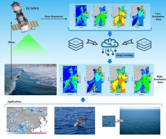
:The analysis of marine environmental parameters plays a significant role in various aspects, including sea surface target detection, the monitoring of the marine ecological environment, marine meteorology and disaster forecasting, and the monitoring of internal waves in the ocean. In particular, for sea surface target detection, the accurate and high-resolution input of marine environmental parameters is crucial for multi-scale sea surface modeling and the prediction of sea clutter characteristics. In this paper, based on the low-resolution wind speed, significant wave height, and wave period data provided by ECMWF for the surrounding seas of China (specified latitude and longitude range), a deep learning model based on a residual structure is proposed. By introducing an attention module, the model effectively addresses the poor modeling performance of traditional methods like nearest neighbor interpolation and linear interpolation at the edge positions in the image. Experimental results demonstrate that with the proposed approach, when the spatial resolution of wind speed increases from 0.5° to 0.25°, the results achieve a mean square error (MSE) of 0.713, a peak signal-to-noise ratio (PSNR) of 49.598, and a structural similarity index measure (SSIM) of 0.981. When the spatial resolution of the significant wave height increases from 1° to 0.5°, the results achieve a MSE of 1.319, a PSNR of 46.928, and an SSIM of 0.957. When the spatial resolution of the wave period increases from 1° to 0.5°, the results achieve a MSE of 2.299, a PSNR of 44.515, and an SSIM of 0.940. The proposed method can generate high-resolution marine environmental parameter data for the surrounding seas of China at any given moment, providing data support for subsequent sea surface modeling and for the prediction of sea clutter characteristics.
1. Introduction
The Marine environment plays a crucial role in the Earth’s ecosystem, with far-reaching impacts on climate patterns and close connections to human production and livelihood [1]. Marine environmental parameters, including waves, wind speed, wind direction, temperature, salinity, etc., play a crucial role in the modeling and understanding of the dynamic changes in the ocean [2,3]. Modeling these marine environmental parameters provides valuable insights into activities occurring both on and beneath the sea. Utilizing ocean environment observation data for modeling enables us to gain a better understanding of the dynamics of the ocean.
The methods for obtaining marine environmental parameters mainly include direct observation methods and advanced remote sensing techniques [4]. Direct observation methods include ship-based observations, buoy observations, and fixed observation stations. These methods collect marine environmental parameters in marine regions, such as sea surface temperature, wind speed, and wave period, to understand changes in the marine environment [5]. Direct observations are typically made by deploying buoys and anemometers on the sea surface. For instance, the China Institute of Radio Propagation placed Datawell Waverider 4 and Lufft WS700-UMB instruments in the Yellow Sea to directly observe marine environmental parameters such as significant wave height, wind speed, and wave period [6]. This observation method enables the acquisition of marine environmental data, providing support for predicting sea clutter characteristics. Direct observation methods are limited by equipment and vessels, which restrict their ability to achieve wide spatial and temporal coverage. Moreover, observations are often intermittent and cannot collect data continuously and in real time. The observed data also have limitations in terms of their temporal and spatial resolutions [7].
On the other hand, remote-sensing technologies, such as satellite remote sensing, airborne remote sensing, and submarine remote sensing, offer the potential to observe the marine environment over larger areas and at higher resolutions [8]. Remote-sensing satellite observation data are typically provided by local or national meteorological organizations [9]. The European Center for Mesoscale Weather Forecasting (ECMWF) [10] has provided global numerical weather forecast data, meteorological reanalysis data, and specific data for various needs since 1979. The ERA-Interim reanalysis data offer oceanic environmental parameter data from January 1979 to August 2019, including wave height, wave direction, wind direction, and wave period. Since August 2019, these reanalysis data have been migrated to the ERA5 database. ERA5 data, in addition to the European Space Agency’s ERS-1/-2 remote sensing satellites and NASA’s QuikSCAT satellite, incorporate various satellite analysis data. The data feature higher spatiotemporal resolution, more accurate hourly estimates of atmospheric variables, and an extensive range of satellite observations, providing valuable support for various research purposes. Our research group utilizes ECMWF data to provide marine environmental parameters for the surrounding marine areas of China (0°N–45°N, 105°E–135°E). We perform multi-scale sea surface modeling [11,12] and analyze sea clutter characteristics [6] in the vicinity of the data collection points to support subsequent sea surface target detection. In order to monitor sea surface targets over larger regions, it is necessary to conduct real sea surface modeling and analysis of sea clutter characteristics over a wide area [13]. Therefore, there is an urgent need to process the marine environmental data provided by ECMWF for the surrounding marine areas of China at a high resolution.
The most common techniques for high-resolution data reconstruction involve using traditional interpolation techniques, such as the nearest neighbor interpolation algorithm, the linear interpolation algorithm, the bilinear interpolation algorithm, the spline interpolation algorithm and the cubic interpolation algorithm. The nearest neighbor interpolation [14] selects the value of the nearest point to the requested data point’s location. This algorithm, however, does not consider the values of other neighboring points, limiting its performance for coarsening purposes. The linear interpolation [15] involves constructing a straight line between the two given points and using it to estimate the unknown value at a point between them. A linear interpolation algorithm may not always be adequate or suitable for contexts that require higher precision or reliability. The spline interpolation [16] fits the spline functions to the available data points and minimizes the overall error or deviation from the underlying trend. However, the spline interpolation algorithm may overfit the data, resulting in a curve that perfectly fits the data but fails to generalize well to new data. The cubic interpolation [17] estimates intermediate values between two known data points by using a cubic polynomial function based on the two adjacent data points. However, when fitting the curve to data points with a cubic polynomial, oscillations may be introduced between the data points, leading to inaccurate and unreliable results. The traditional methods have been widely adopted for their simplicity and computational efficiency. However, these methods often struggle to achieve superior performance in terms of effectiveness.
Currently, high-resolution reconstruction methods commonly rely on image-based approaches [18,19,20,21]. These methods show limited effectiveness in reconstructing edge details for the data used in this study, with little improvement compared to traditional methods, but requiring more computational time. Recently, some researchers proposed deep learning-based high-resolution methods for ocean environmental parameters. For example, Aurelien et al. [22] employed the SRCNN model for the high-resolution reconstruction of sea surface temperature and conducted experiments with different parameters of the SRCNN model. Similar to SRCNN, they encountered difficulties in accurately reconstructing the fine details of the data. Wang et al. [23] applied the LightGBM algorithm to establish a model for the high-resolution reconstruction of sea surface salinity data. They also pointed out that the reconstruction results of the proposed method in certain sea areas of China were unsatisfactory. Su et al. [24] utilized two methods, a convolutional neural network (CNN) and a light gradient boosting machine (LightGBM), to reconstruct high-resolution deep-sea temperature data. The time-series CNN model achieved better performance. But due to the use of a shorter time series, the reconstruction accuracy was not very high, and it did not focus on reconstructing the details of the data.
To enhance the focus on specific features at particular positions, attention mechanisms have been introduced in various fields of artificial intelligence, such as visual captioning [25], scene segmentation [26], semantic segmentation [27], machine translation [28,29], text classification [30], speech recognition [31], and time-series analysis [32], within different CNN architectures. The attention mechanism works similarly to the human brain’s attention process [33]. The attention mechanism makes the model focus on a specific part or feature in the input and assigns different weights according to its importance in the task. Hu et al. [34] proposed SENet, which combines channel attention and channel-wise feature fusion to suppress unimportant channels. However, its effectiveness in suppressing unimportant pixels is limited. Woo et al. [35] introduced spatial attention, combining channel attention and spatial attention. However, they overlooked the channel–spatial interactions and lost information in the process. Misra et al. [36] utilized attention weights between the channel, spatial width, and spatial height dimensions to improve efficiency. However, attention operations were still applied to two dimensions at a time. Liu et al. [37] proposed the global attention mechanism (GAM) module in the field of image classification, which is capable of capturing important features across three dimensions, enabling focusing on important information and the suppression of unimportant information. Chen et al. [38], in the person re-identification (ReID), observed that most attention mechanisms fail to adequately capture the fine-grained details of input features. They introduced the high-order attention (HOA) module, which utilizes a high-order polynomial predictor to capture subtle variations among the data.
In this study, we introduce two attention modules to enhance attention on edge details: the GAM attention module [37] and the high order attention (HOA) module [38]. The GAM module is more effective in enhancing the network’s attention for specific features, which is used in the feature extraction part; the HOA module is capable of capturing more fine-grained features, which is used in the feature refinement part. The network has successfully increased the resolution of the input marine environmental parameters by two or four times, and it can be further extended to achieve even higher resolutions in the future.
The rest of this paper is organized as follows. Section 2 describes the method used in this paper. In Section 3, the optimal settings selected according to the different experimental setups are presented. Section 4 verifies the effectiveness by comparing it with traditional interpolation methods. Section 5 discusses the results and explores future research directions. Section 6 summarizes our research findings.
2. Methodology
The structure of a network and its constituent modules play a crucial role in the effective functioning of any network. In this section, we explain the design of the network we have employed in this article and highlight its major components.
2.1. Network Structure
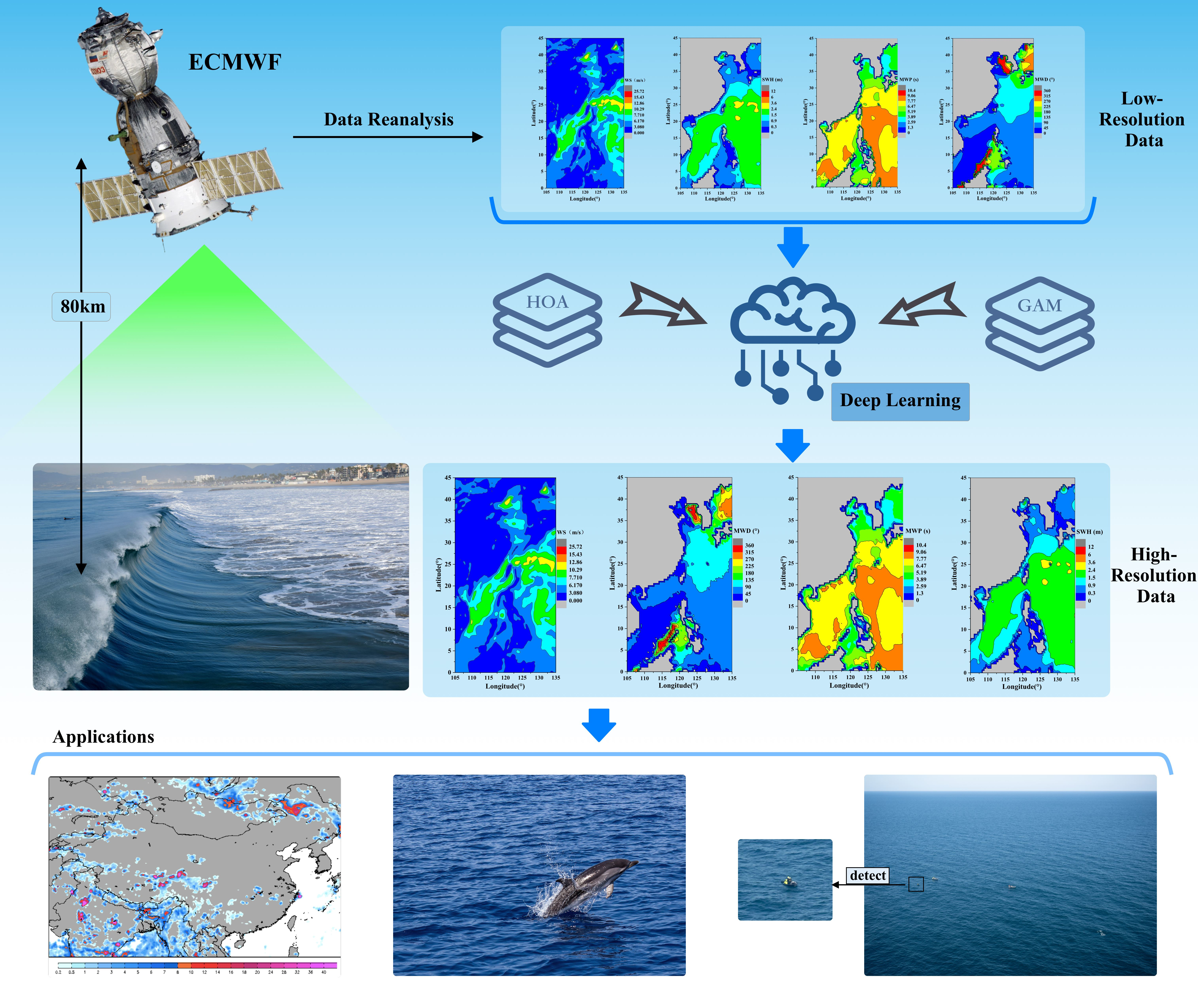
As shown in Figure 1, the network used in this study mainly consists of a feature extraction part and a feature refinement part. The initial features are first extracted from the low-resolution input data. The results are passed into a GAM module; the results from the GAM module are then input to the HOA module, along with the results from the prior residual structure for feature refinement; and finally, the reconstructed high-resolution data are output through the upsampling part.
The feature extraction network uses several feature connection groups to form the residual structure, and then the residual results are fed into the GAM module to extract features. In this paper, weighted channel cascade (WCC), a new network connection technique similar to the structure utilized in [39], is used in place of a straightforward element summing connection. The results, which are based on the Conv-ReLU-Conv structure, are fed into a 1 × 1 convolutional layer using the WCC connection to form a residual block, and the results of the residual block are fed into the 1 × 1 convolutional layer with the original input through the WCC connection, thus forming a residual group. In addition, the residual group forms the part of the feature extraction using the Conv-ReLU-Conv structure with WCC concatenation.
Since the resolution of the data used in this paper is low, the feature refinement part has a simple structure, using only one HOA module for the connection. An HOA module is used for the edge part, and an HOA module is used for the non-edge part. This is then fed into an upsampling layer to obtain high-resolution data.
2.2. Attentional Mechanisms
After observing the data, it was found that the reconstruction of the edge part of the results obtained by extracting features only through convolutional layers is poor, sometimes even worse than the results of traditional interpolation methods. In order to improve the feature extraction and refinement of the edge parts, we add two attention modules to the network used in this article.
2.2.1. GAM Module
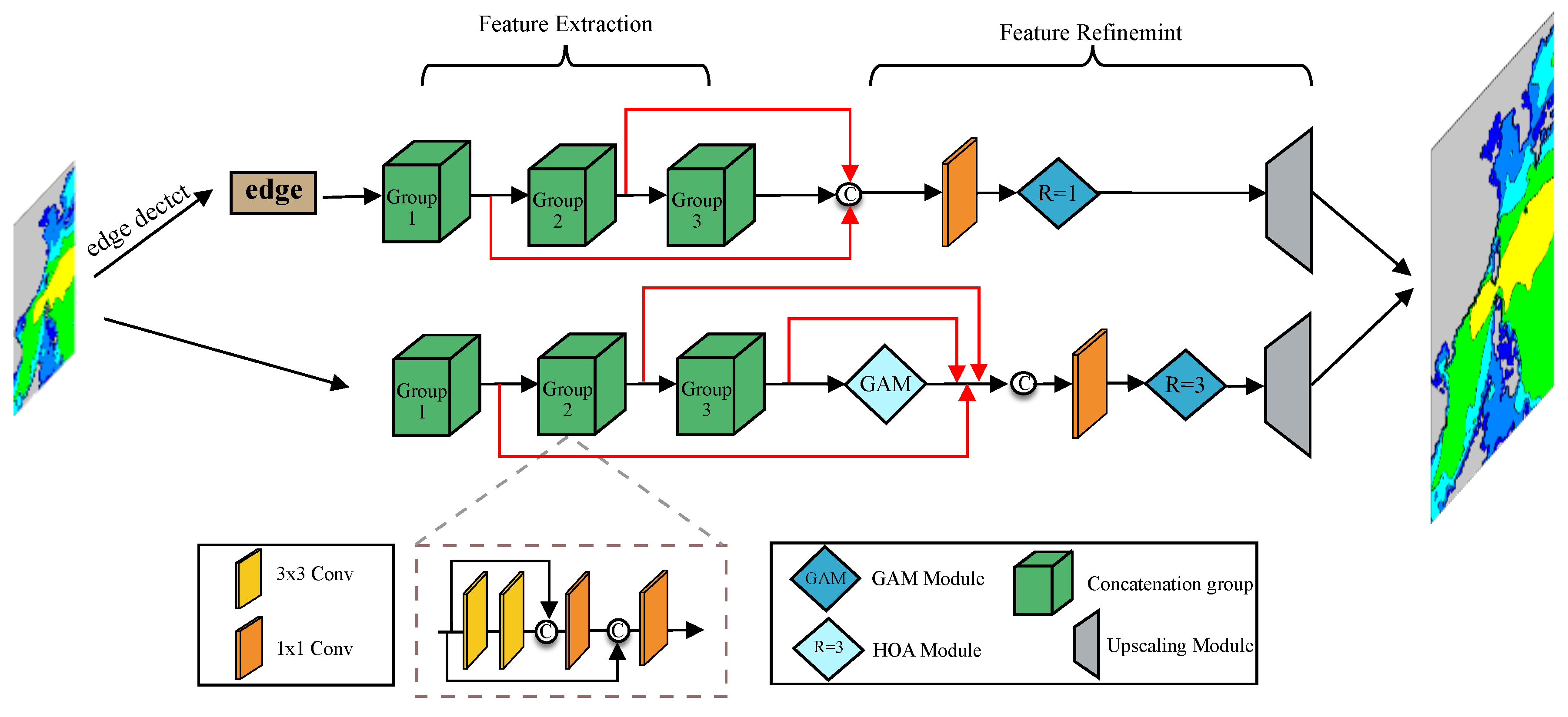
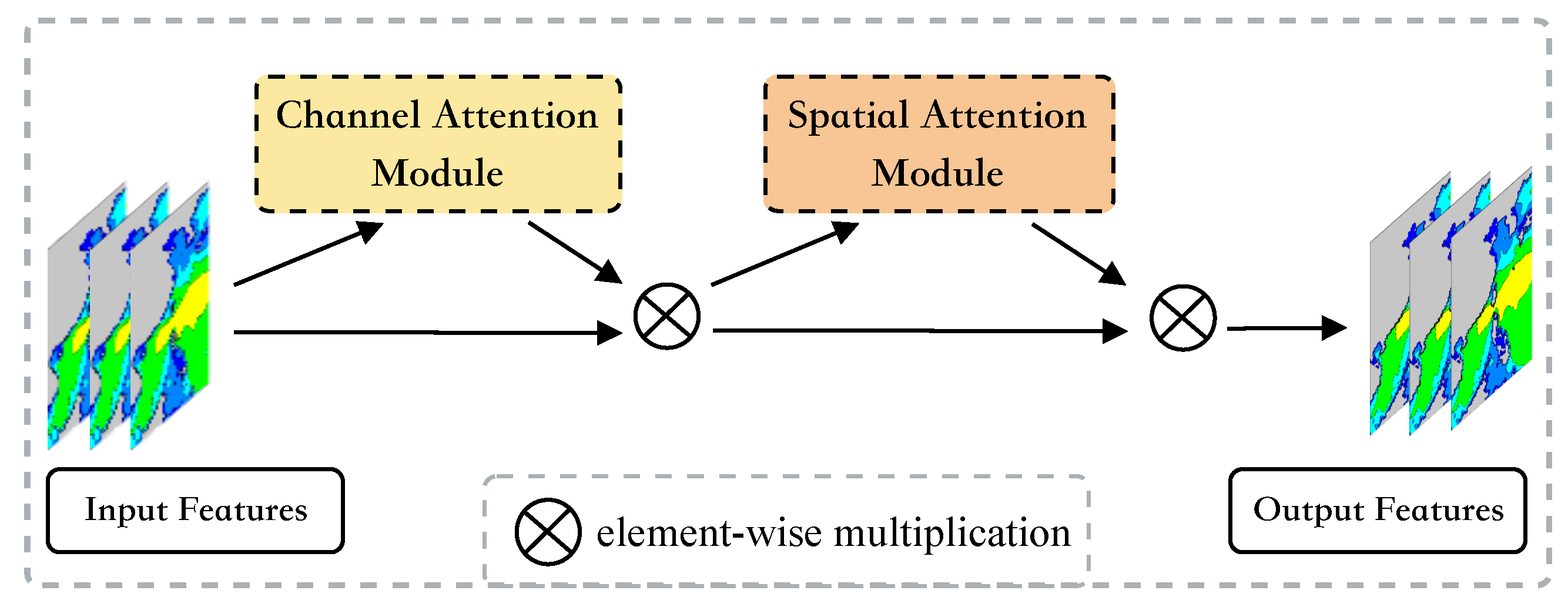
Figure 2 depicts the GAM module employed in this paper. It can be seen that the GAM module leverages the channel attention mechanism and the spatial attention mechanism.
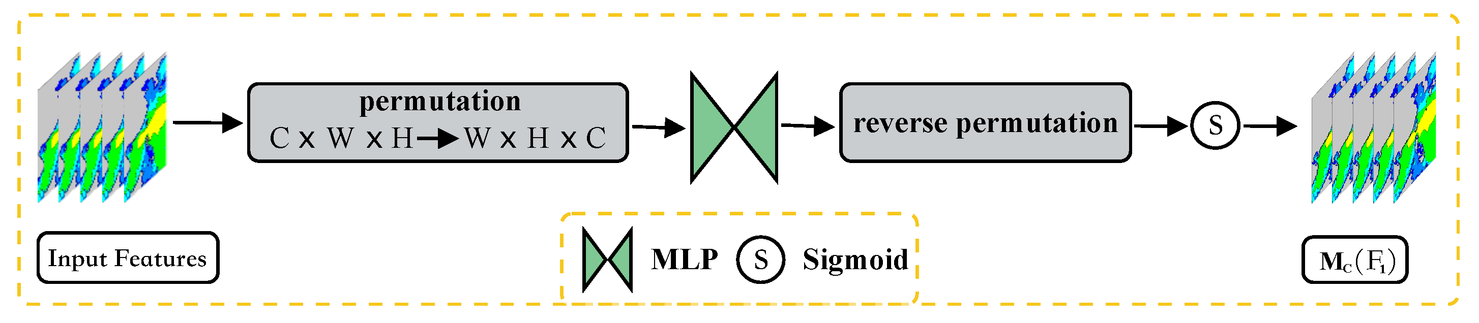
To elucidate the functionality of the channel attention mechanism employed in the GAM module, Figure 3 provides a schematic representation. A dimension transformation is performed on the input feature map before feeding it into the multilayer perceptron (MLP) [40]. Then, the transformed feature map is converted back to its original dimension and processed through sigmoid activation before being outputted. The resulting feature maps are enriched with informative channel-wise representations that contribute to the task performance.
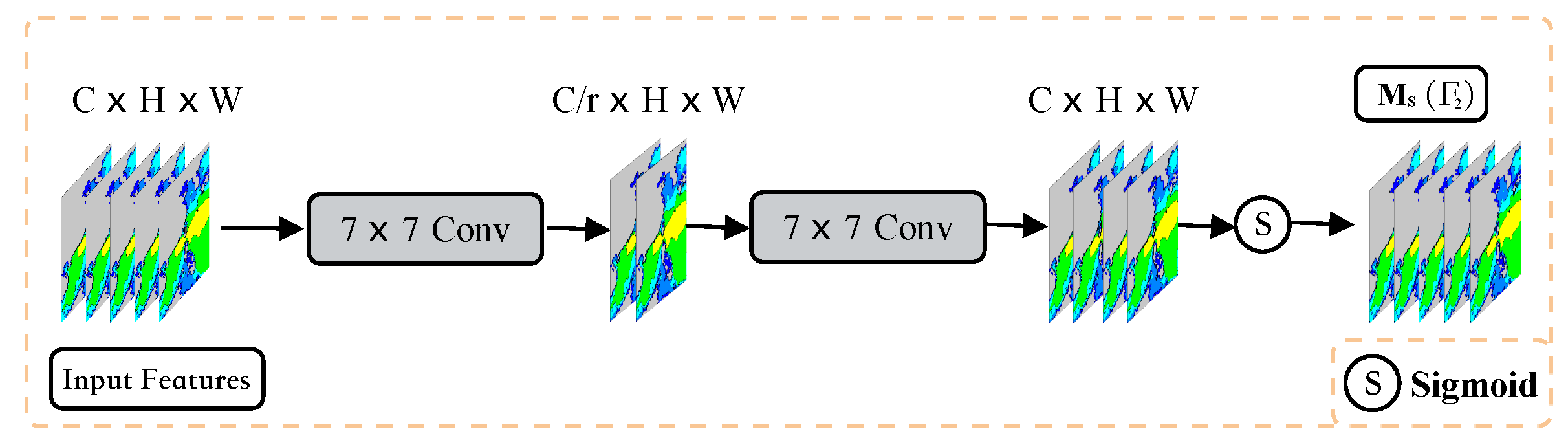
Figure 4 illustrates the spatial attention mechanism employed in the GAM module. The spatial attention mechanism employs convolution processing [41] to enhance its performance. This is achieved by reducing the number of channels through a convolution kernel, which reduces the computational requirements. The resulting feature maps are then increased back to their original channel count and outputted via the sigmoid activation function. To ensure maximum information utilization, the max pooling operation is eliminated from the process. These modifications significantly improve the network’s performance by enriching the feature maps with more informative spatial representations.
2.2.2. HOA Module
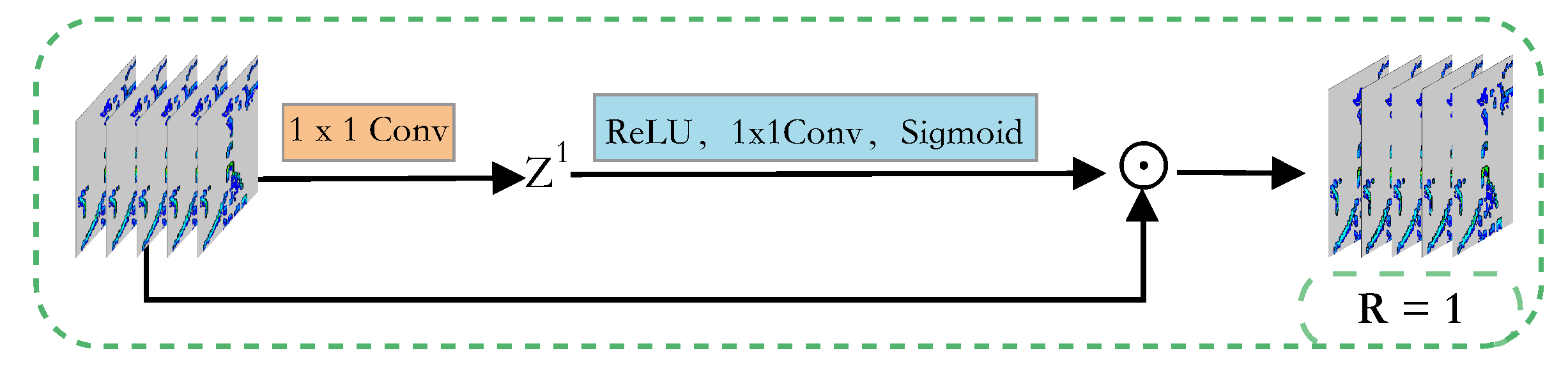
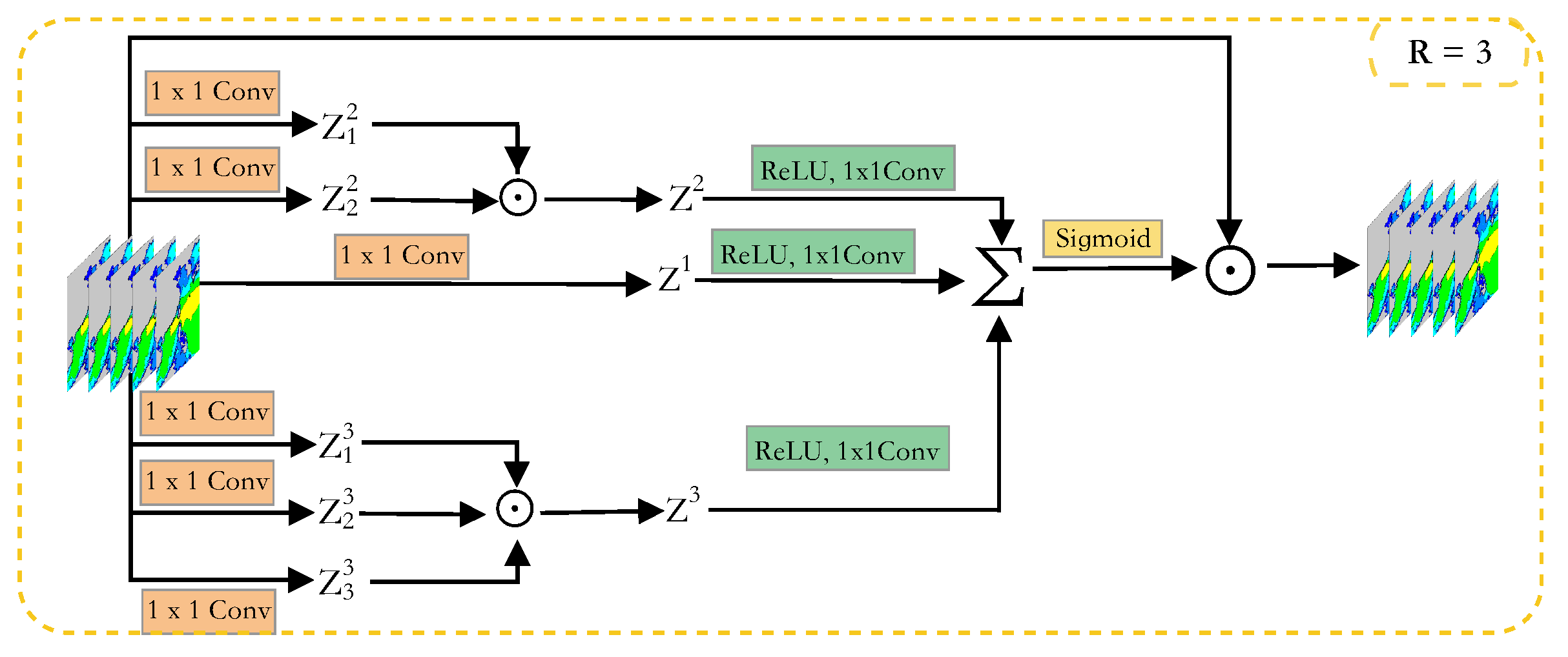
The figures, namely Figure 5 and Figure 6, illustrate the cases of R = 1 and R = 3 in the HOA module.
Given an input feature X, which is a 3D tensor with C channels, H height and W width, it is fed into R 1 × 1 convolutional layers to obtain R intermediate features , where each is also a tensor of size . Similarly, at level , are obtained through 1 × 1 convolutional layers. From level R to level 1, a total of Z are generated. For every level, combine the generated to obtain :
where , , ⊙ is elementwise product. Then, add the generated to the ReLU activation function and a 1 × 1 convolutional layer, and combine the obtained features into the sigmoid activation function, which can be expressed as
where is the ReLU activation function and a 1 × 1 convolutional layer. Finally, similar to other attention mechanisms [42], multiply the received by the input feature X to obtain the final output.
Within the HOA module, an increase in the variable R leads to a corresponding increase in the quantity of information attainable. This, in turn, provides the model with a greater overall capacity for effective representation.
3. Experiments
3.1. Settings
Data on marine environmental parameters used in this study were taken from the European Center for Mesoscale Weather Forecasting (ECMWF) for coastal waters in China (0°N–45°N, 105°E–135°E). The daily sampling interval of the data is 1 h. The parameters include mean wave direction (MWD), significant wave height (SWH), mean wave period (MWP), 10 meter U wind component (U10) and 10 meter V wind component (V10). In order to obtain wind speed (WS) data, u10 and v10 need to be preprocessed in advance:
Due to U10 and V10 both having a spatial resolution of 0.25°, the spatial resolution of WS remains unchanged at 0.25°. Moreover, the spatial resolution of MWD, SWH and MWP is 0.5°. Some properties of these datasets are shown in Table 1. To account for the effects of time on certain marine environmental parameters, the training data consist of four parameters, each with 8186 data points, taken from all time points between January and April of 2016 to 2020. The test data still include these four parameters, each with 41 data points, taken from all time points between 21 and 23 January 2021. Before training, the training data are also expanded by 90° rotation, horizontal and vertical flipping, and enlargement.
In this paper, low-resolution data are generated using three methods: alternate downsampling (alternately select values from rows and columns), maximum downsampling, and average downsampling. The data were downsampled by scale factors of 2 and 4. Table 2 displays some properties of the datasets. The downsampled data are used as the input for the high-resolution reconstruction model.
After comparing several classic optimization approach, the model parameters were updated using the Adam optimization approach [43], with 1 and 2 set to 0.9 and 0.999, respectively. The learning rate was initially set at 0.001, with a tenfold reduction for each of the following 50 epochs and the remaining unchanged for the final 50 epochs. An NVIDIA GeForce RTX 3090 GPU and CUDA 11.4 were used in this paper.
3.2. Loss Function
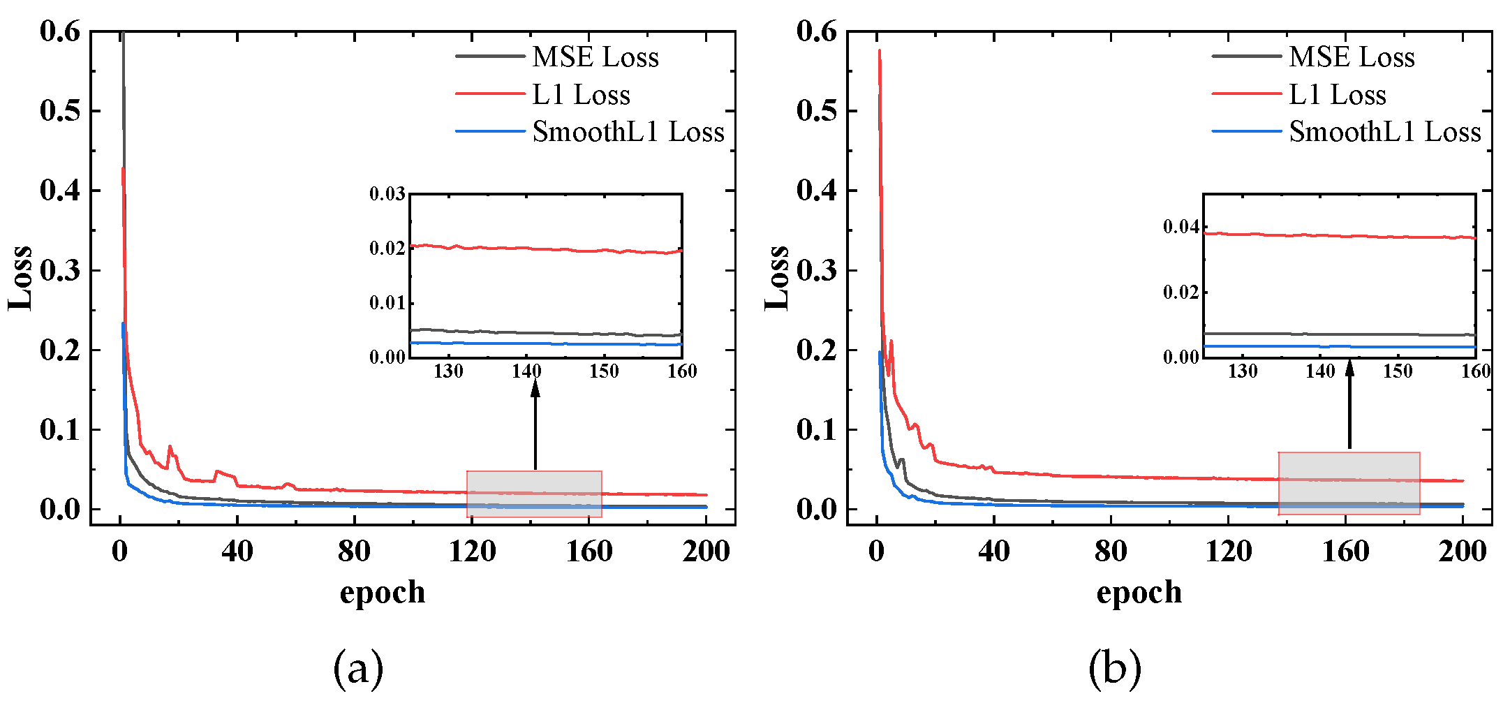
In this paper, the following three loss functions are tested, and the convergence effect of loss is compared to select the loss function with the best convergence effect:
- MSE loss function [44]. Given the same input data x, the MSE loss function can be formulated aswhere N is the total training data, is the true output of the input data x, and is the predicted output of the input data x.
- SmoothL1 loss function [46]. Given the same input data x, the SmoothL1 loss function can be formulated as
Figure 7 shows the comparison of the loss function convergence effects. We conducted the experiments with our method with different loss functions and data downsampled with the same downsampling method and compared the results at various high-resolution scales.
From Figure 7, it can be seen that the model loss performs best when using the SmoothL1 function as the loss function. Therefore, the SmoothL1 loss function is chosen as the loss function for training.
3.3. Evaluation Criteria
In this paper, three commonly used evaluation criteria are used to compare the experimental results, which are the mean squared error (MSE) [47], the peak signal-to-noise ratio (PSNR) [48], and the structural similarity index measure (SSIM) [49]:
- The MSE measures the average squared difference between the estimated values and the actual value. Given an actual value and predicted value , the MSE value is
- The PSNR is an objective criterion for evaluating images and is used to measure the difference between two images. Given an actual value Y and predicted value , the PSNR value isThe max value is the maximum possible pixel value of the given value, usually 255. The higher the PSNR value, the better the reconstruction effect of the estimated image and the higher the similarity to the actual image.
- The SSIM is used to measure the similarity between two images. Given an actual value Y and predicted values , the PSNR value iswhere () represents the pixel sample mean of Y (), () represents the variance of Y (), and is the covariance between Y and . Compared with the MSE and PSNR, the SSIM is closer to the human visual system. The higher the SSIM value, the higher the similarity between the two images.
3.4. Traditional Method
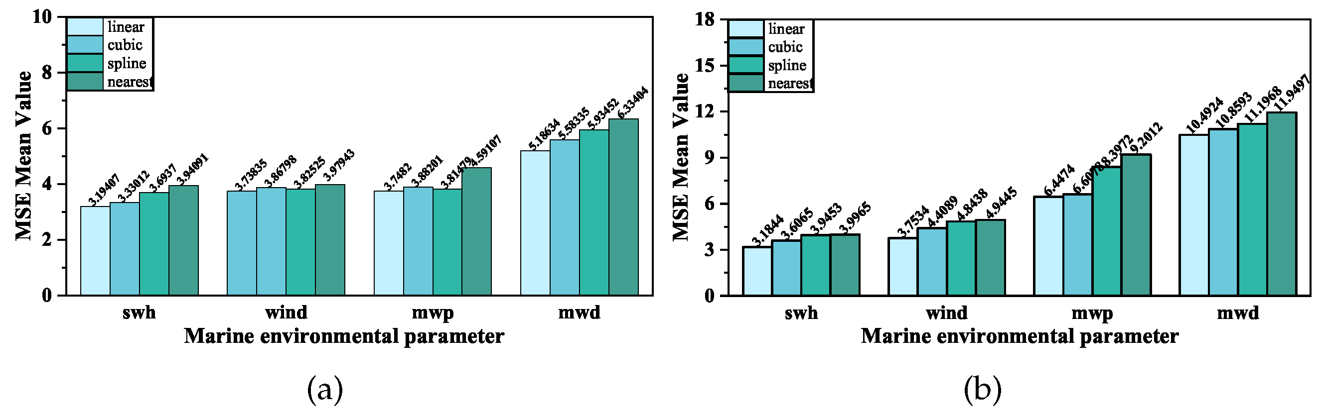
In this paper, the MSE results of four traditional interpolation methods are compared: the nearest neighbor interpolation algorithm, the linear interpolation algorithm, the spline interpolation algorithm, and the cubic interpolation algorithm. The results are displayed in Figure 8. Based on these experiments, the best traditional interpolation method is chosen for comparison.
Figure 8 shows a comparison of the MSE results for four interpolation algorithms. The results indicate that the linear interpolation algorithm achieves the smallest MSE. Thus, in this paper, the linear interpolation algorithm will represent traditional interpolation algorithms and compare with the proposed model.
3.5. Downsampling Method
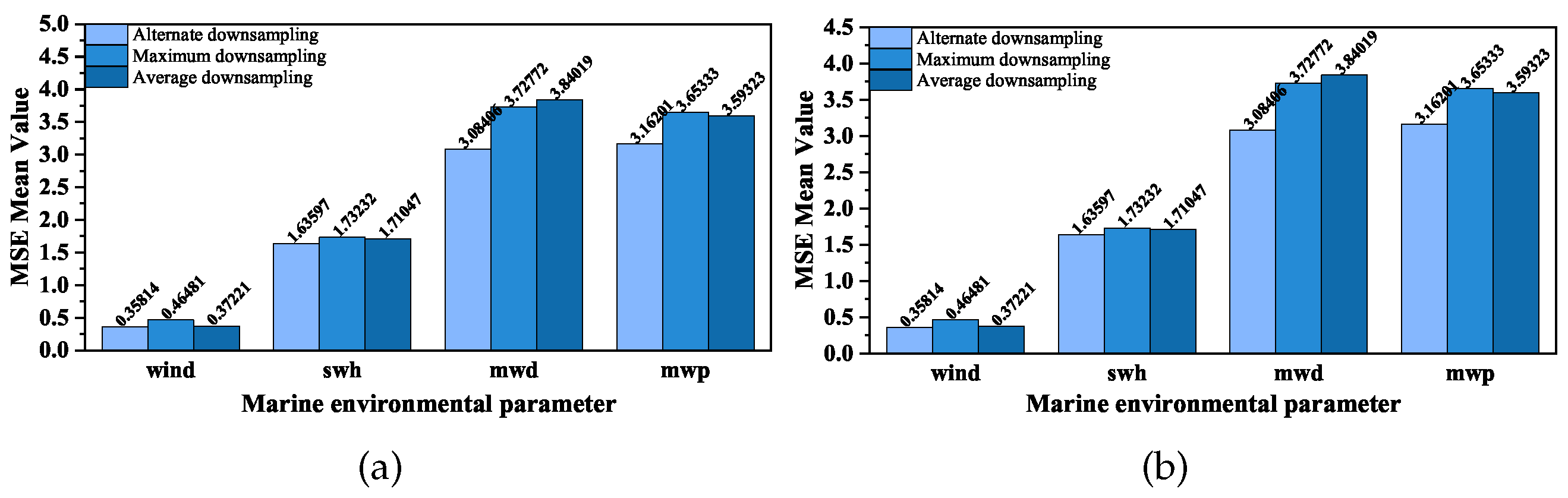
To determine which downsampling method loses the least amount of detail, we compared three downsampling methods: alternate downsampling, maximum downsampling, and average downsampling. We conducted experiments using data downsampled with different downsampling methods and compared the results at various high-resolution scales. The results are displayed in Figure 9. Based on these experiments, the most effective downsampling method is chosen for training. A comparison is made of mean MSE values for different downsampling factors using the same down-sampling method on various marine environmental parameters.
Figure 9 shows that alternate downsampling minimized the mean MSE value between the data obtained by the model and the original data. However, there were instances where average downsampling exhibited a lower mean MSE value. Therefore, in the following text, the results of using both downsampling methods are used as representatives of this model and are compared with traditional methods.
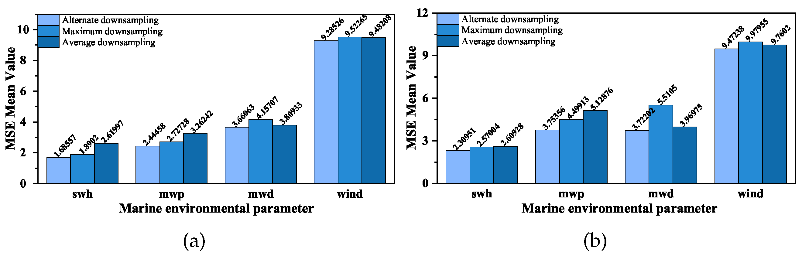
Figure 10 compares the mean MSE value of traditional interpolation methods when using different downsampling methods. The figure shows that for different marine environmental parameters, the best results are obtained when the data are downsampled using the alternate downsampling method. Therefore, when applying traditional interpolation algorithms to the data in the following text, we choose data that have been downsampled using the alternate downsampling method for interpolation.
3.6. Ablation Study
This section introduces a series of experiments to verify the validity of the modules utilized in this paper. First, a baseline model without attention modules is evaluated, and it is predominantly comprised of three convolutional layers, one activation layer, one pooling layer, and one upsampling layer. Then, we conduct the experiment with only the GAM module. Experiments are then conducted to study the impact of HOA modules with different orders, including 1 to 3 HOA modules; to HOA modules; HOA module; HOA module; and HOA module. Finally, we experimentally study the modules presented in this paper, including the 3 HOA module and the GAM module. All experiments maintain the same experimental settings, except for the network architecture. The evaluation metrics used are the MSE, PSNR and SSIM mentioned earlier, the results of which are shown in Table 3. The evaluation process involves a comparison of images rather than a direct comparison of data.
From Equations (7)–(9), it can be inferred that a smaller MSE value indicates a smaller deviation between the data, a larger PSNR value implies a smaller discrepancy between images, and a larger SSIM value indicates higher image similarity. From Table 3, it can be seen that incorporating HOA modules into the network yields improved performance compared to the baseline model without HOA modules. The model with only one GAM module performs worse than the models with one HOA module or one HOA module. Regarding the number of HOA modules, a network with only one HOA module performs better than those with two or three. As for the order of the HOA module, a network with one HOA module outperforms those with one HOA module and one HOA module. The network architecture proposed in this paper, consisting of one HOA module and one GAM module, achieves the highest performance.
4. Comparison
4.1. Assessment in Terms of Different Metrics
The evaluation metrics results of the reconstruction effects achieved by different methods are shown in Table 4.
From Table 4 above, it can be seen that the model results obtained in this paper are always better than traditional interpolation methods. The WS achieves the highest PSNR value of 49.598, indicating a minimal disparity between the obtained result and the original image. Similarly, the highest SSIM value of 0.981 confirms the visually impressive quality of the obtained outcome. Other parameters also exhibit PSNR values above 42 and SSIM values above 0.910. In the case of the MWD, the overall result is less satisfactory compared to other parameters. This observation can be attributed to the inherent distribution characteristics of the data. Future improvements will be implemented to address this limitation. For the method proposed in this paper, the alternate downsampling method generally yields superior results. It is worth noting that certain cases, such as MWP, exhibit better results when employing the average downsampling method.
4.2. Visual Results
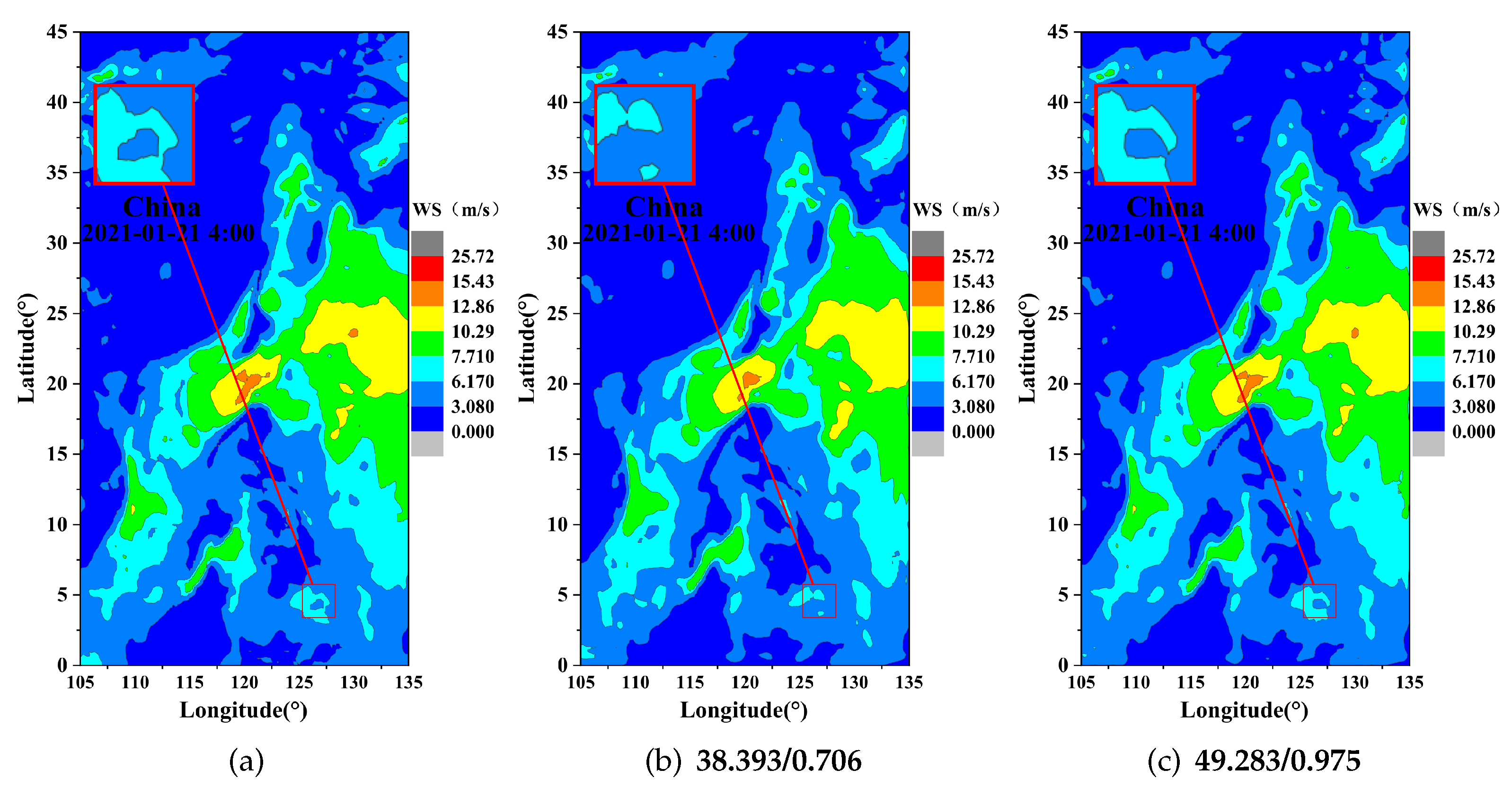
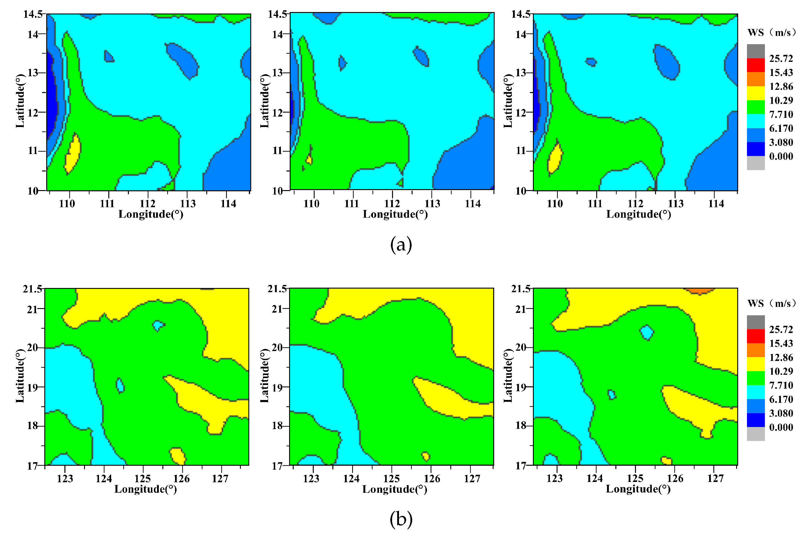
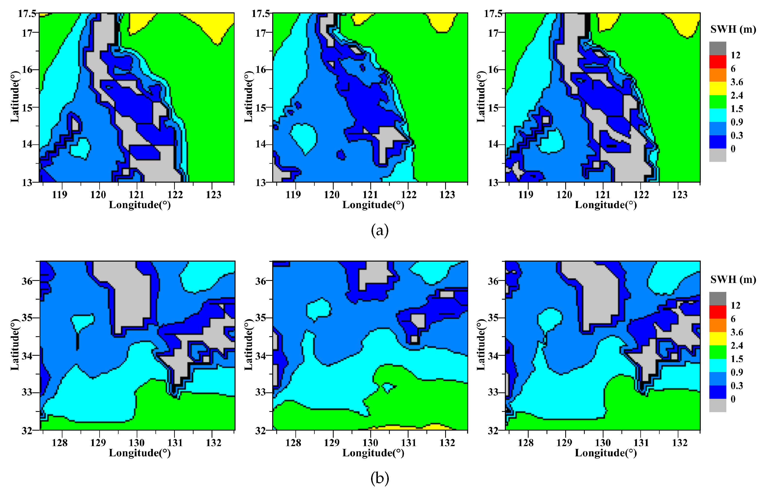
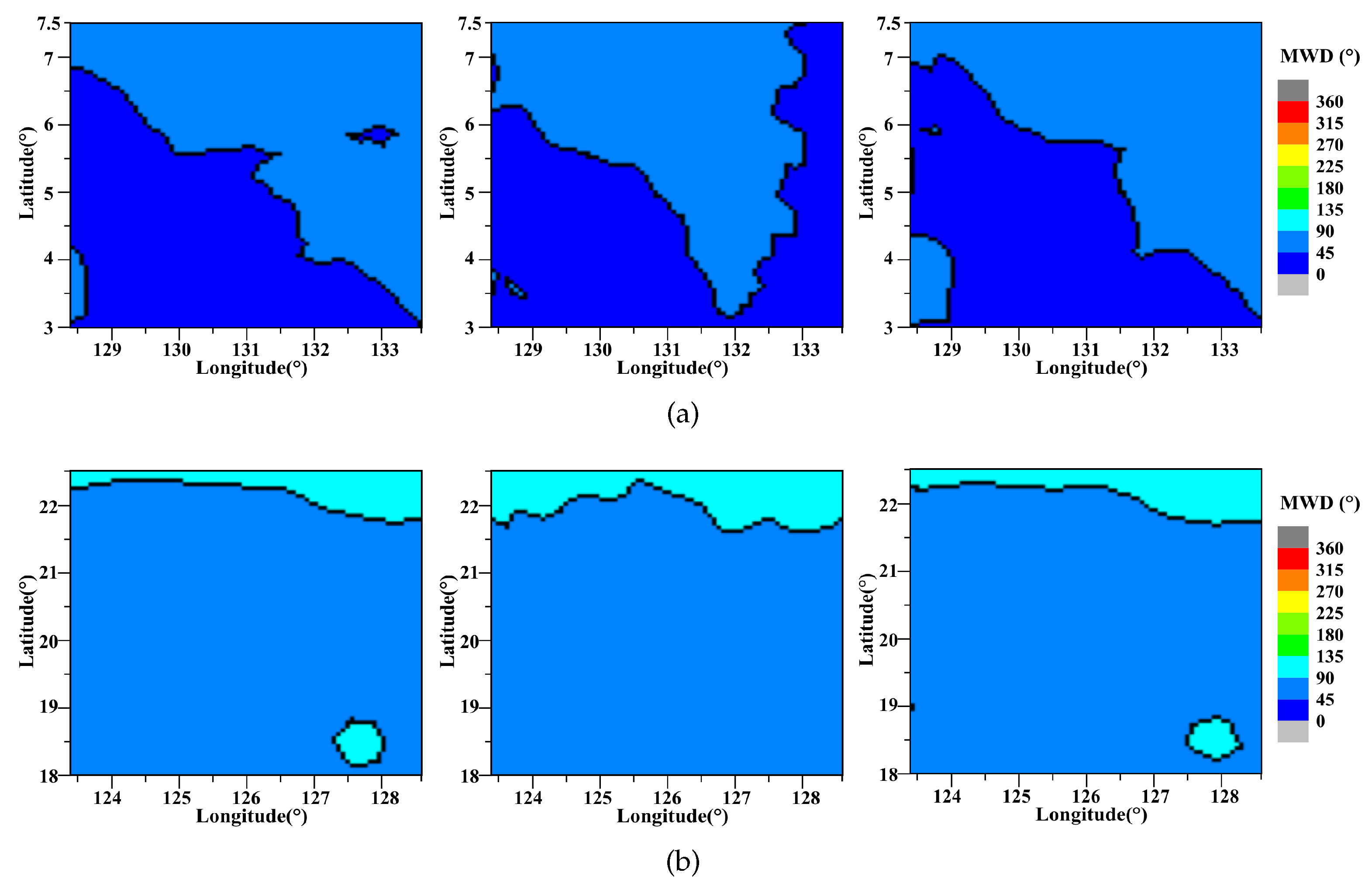
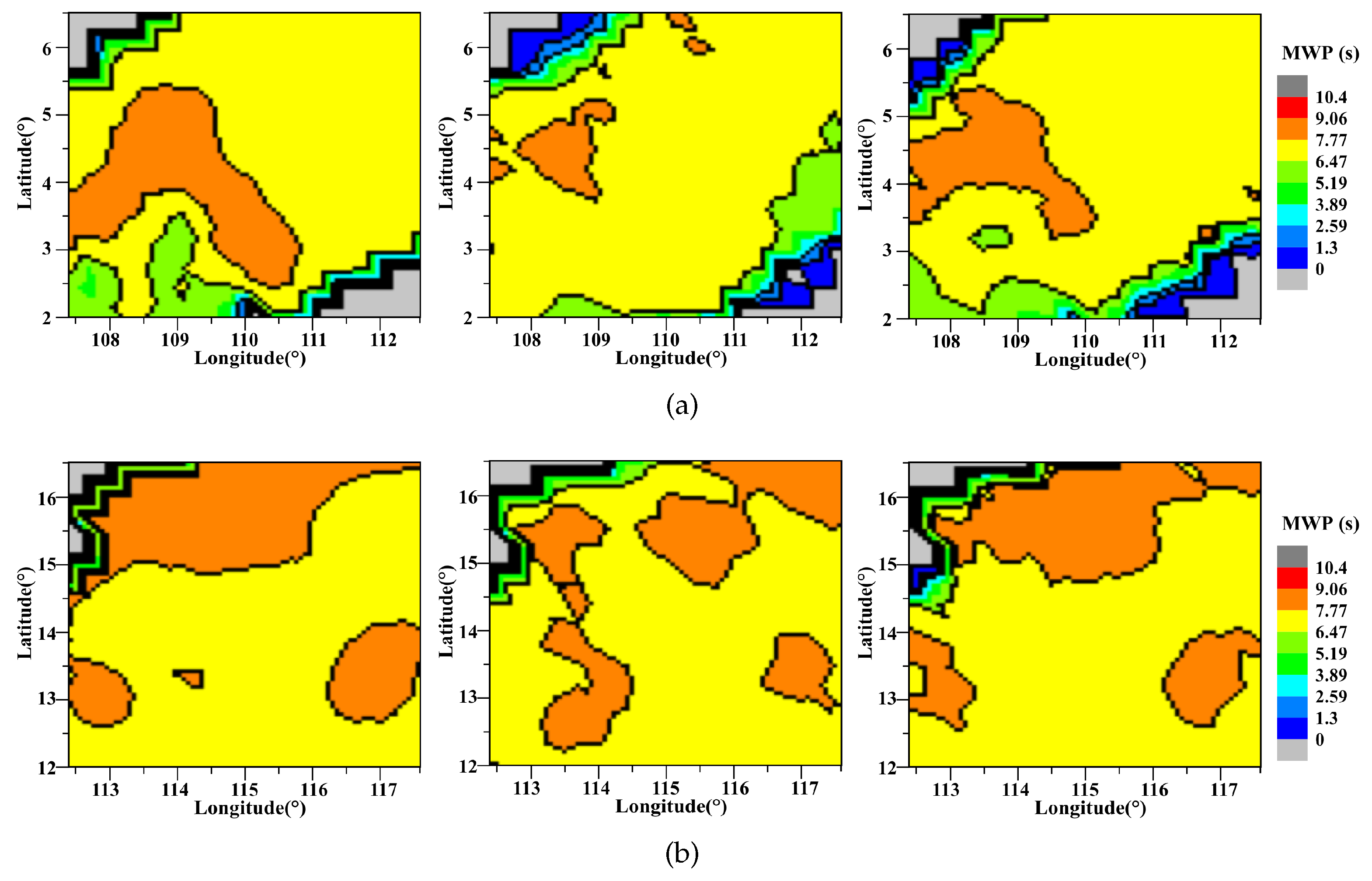
Referring to Table 4, we give the MSE, PSNR and SSIM values of each class in detail. The following Figure 11, Figure 12, Figure 13, Figure 14, Figure 15, Figure 16, Figure 17 and Figure 18 show the qualitative results of different reconstruction methods for the given data. For visual analysis, the reconstructed data are presented as graphs. The colors in the image represent the magnitude of the data, with different color distributions for each parameter. Overall, darker colors indicate larger data values. We mark out the positions that display obvious distinctions among different methods.
From Figure 11, it can be observed that our method closely resembles the distribution of the original data. Clearly, at the time point of 2021-01-21 4:00, when the high-resolution scale is 2×, our method reconstructs the distribution of the fine details of the original data, with a PSNR of 49.283 and an SSIM of 0.975.
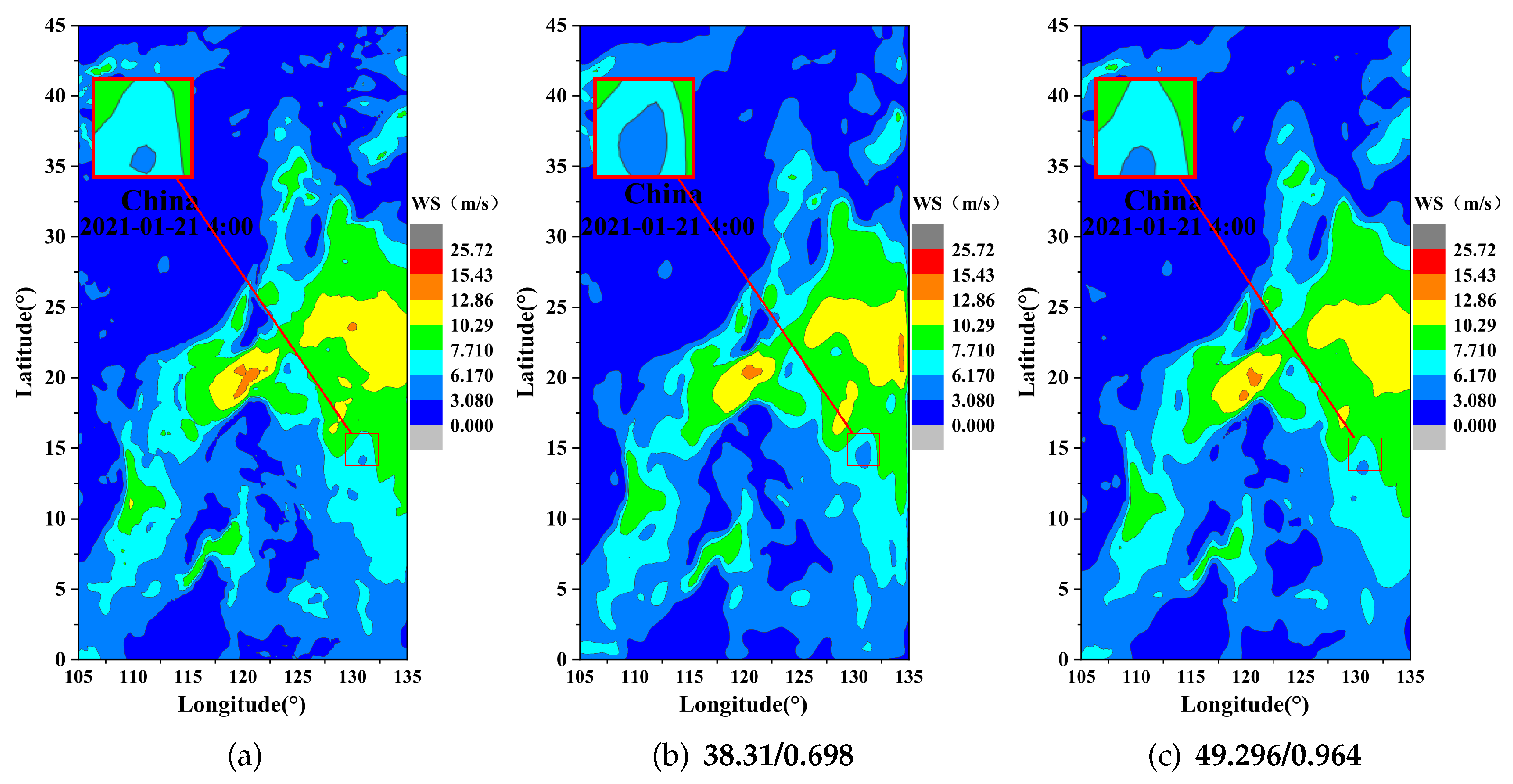
From Figure 12, it can be observed that our method accurately reconstructs the edge distribution of the data, while interpolation methods tend to amplify the edge portions. At the time point of 2021-01-21 4:00, when the high-resolution scale is 4×, our method’s reconstruction result exhibits a closer resemblance to the edge distribution of the original data, with a PSNR of 49.296 and an SSIM of 0.964. Overall, the results of the 2× high-resolution reconstruction are better. The 4× high-resolution reconstruction, compared to the 2× reconstruction, still misses some details.
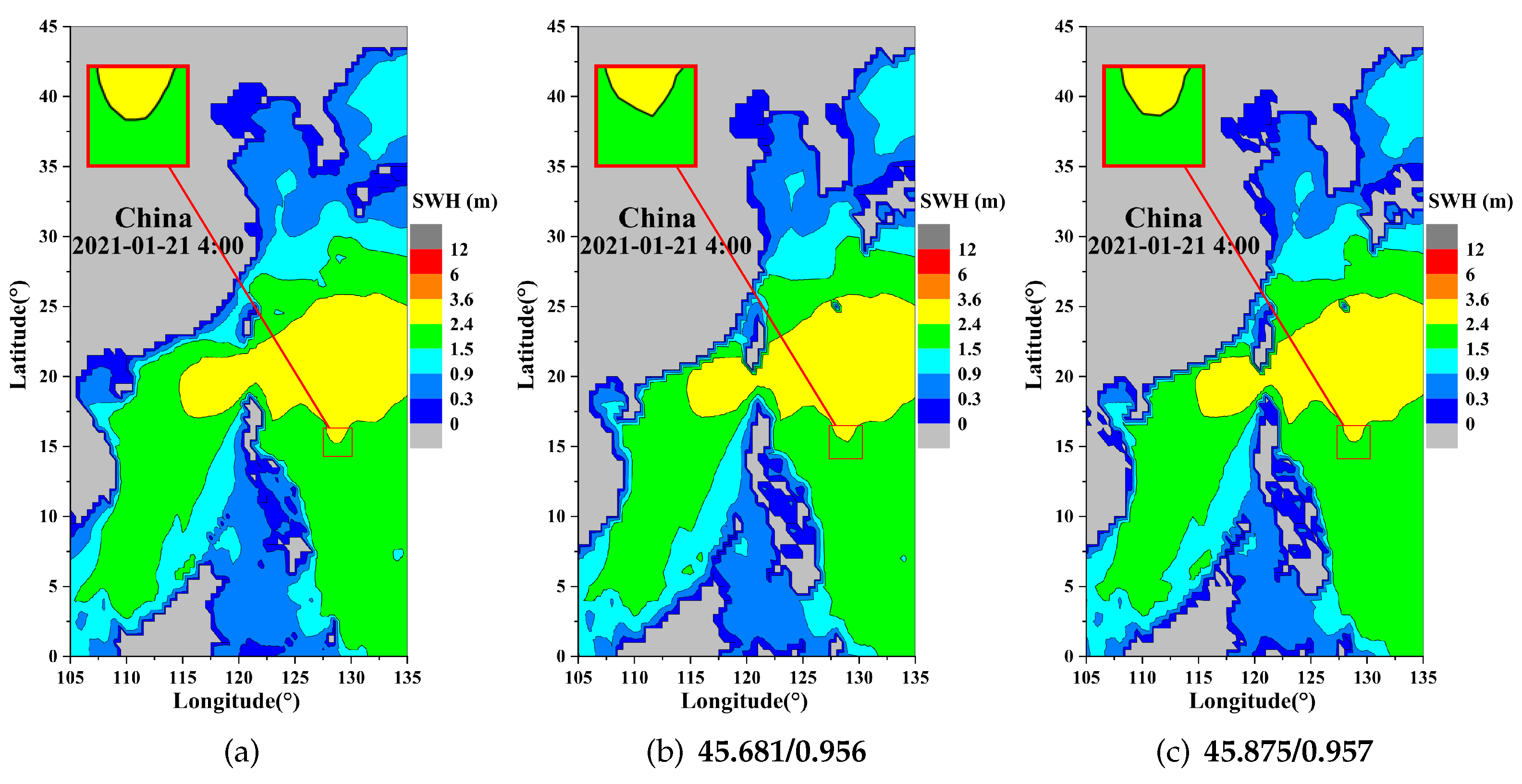
From Figure 13, it can be observed that our method achieves superior results when the high-resolution scale is 2×, with a PSNR of 45.875 and an SSIM of 0.957 at the time point of 2021-01-21 4:00. It is noticeable that across all methods, the reconstruction effects for certain parts are not ideal and introduce some data that do not exist in the original data. This observation may be attributed to the inherent distribution characteristics of the data itself.
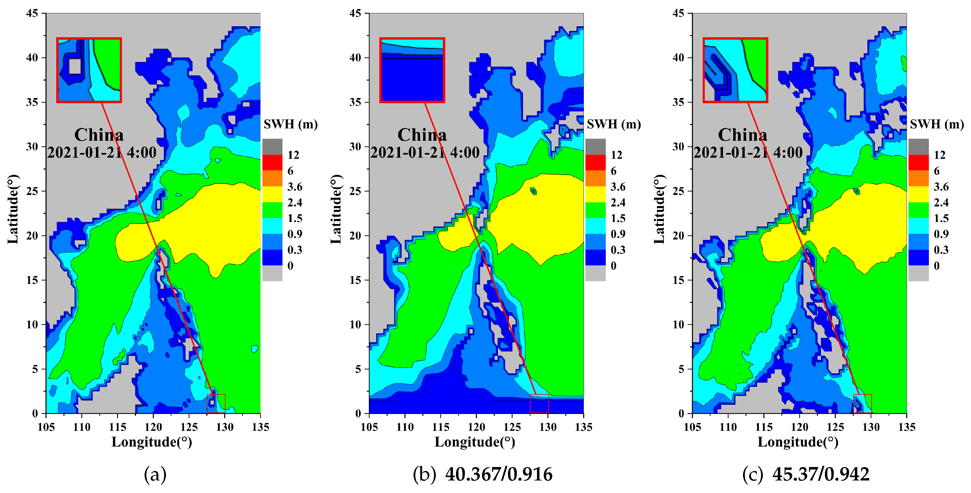
From Figure 14, it is evident that our method produces better results when the high-resolution scale is 4×. Interpolation methods perform poorly in reconstructing certain regions, while our method accurately reconstructs this portion of the data. Our method achieves a PSNR of 45.37 and an SSIM of 0.942 at the time point of 2021-01-21 4:00. Overall, the results of the 2× high-resolution reconstruction are better.
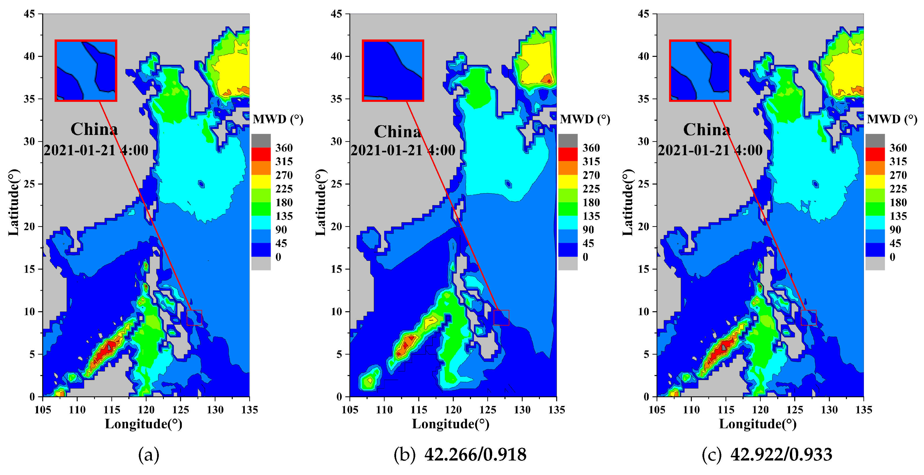
From Figure 15, it is evident that our method produces better results when the high-resolution scale is 2×, displaying a higher resemblance to the edges of the original data. Our method’s reconstruction results closely align with the distribution of the original data, with a PSNR of 42.922 and an SSIM of 0.933 at the time point of 2021-01-21 4:00. The interpolation method, on the other hand, shows mediocre performance and is not accurate enough to capture both the overall distribution and the fine details of the data.
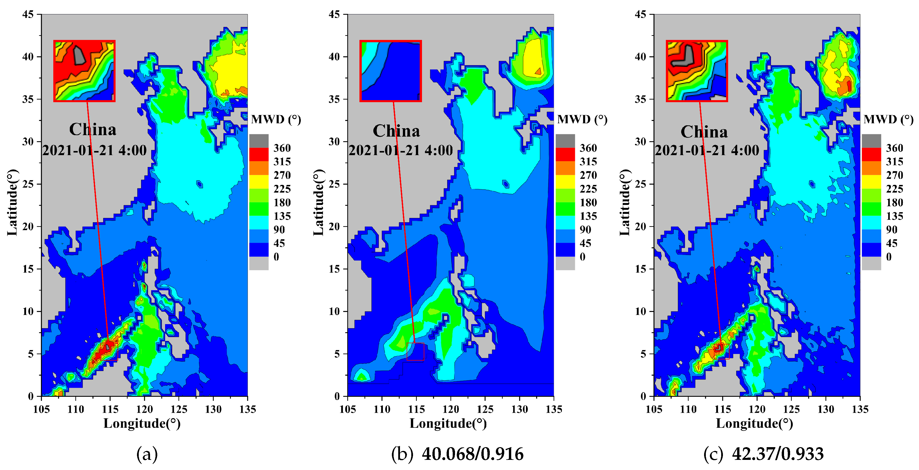
From Figure 16, it is evident that our method accurately reconstructs certain details of the data when the high-resolution scale is 4×, while the interpolation method performs worse. Our method achieves a PSNR of 42.37 and an SSIM of 0.933 at the time point of 2021-01-21 4:00. Similarly, the 4× high-resolution reconstruction results are poorer compared to the 2× high-resolution reconstruction, with inaccurate data distribution in certain regions.
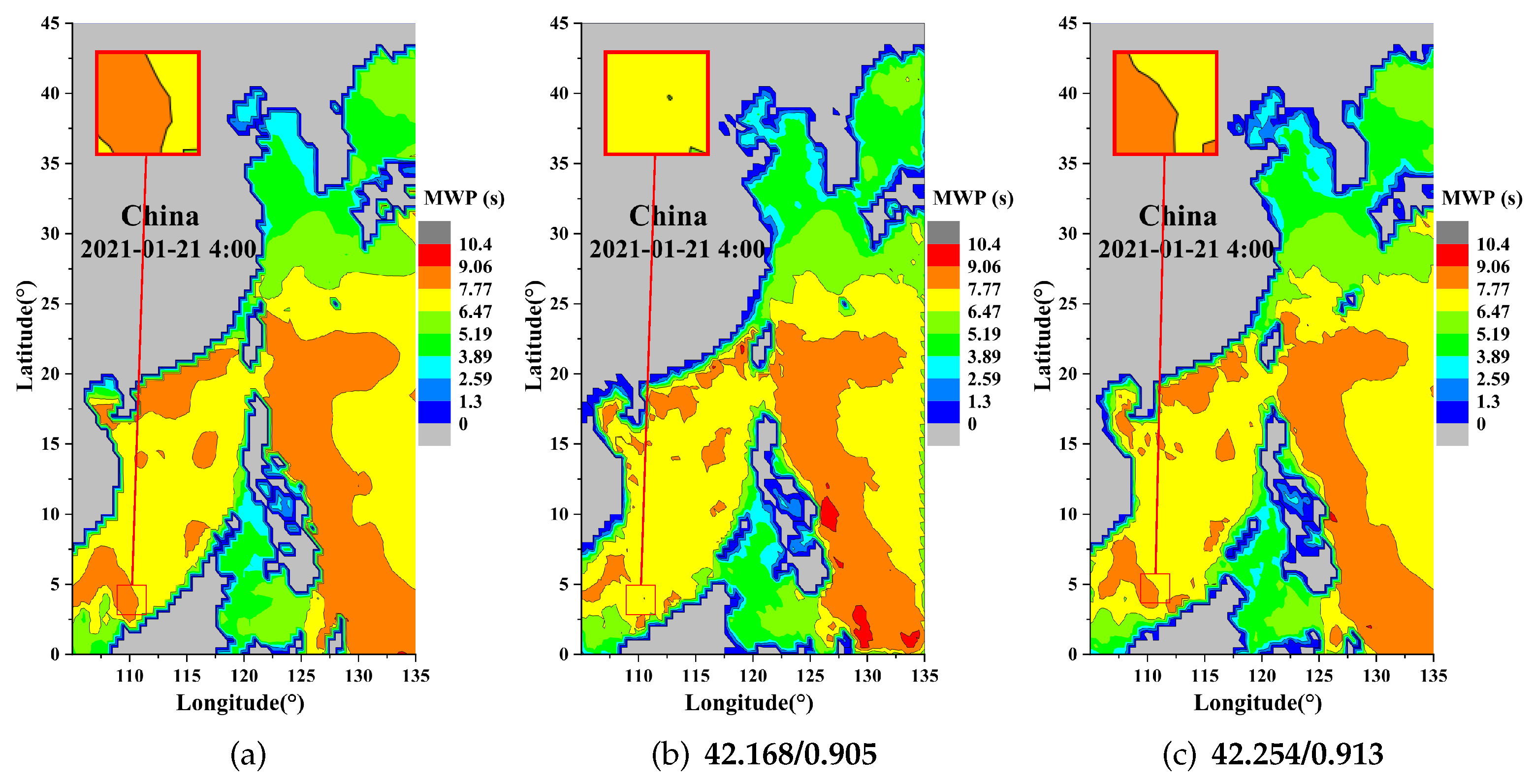
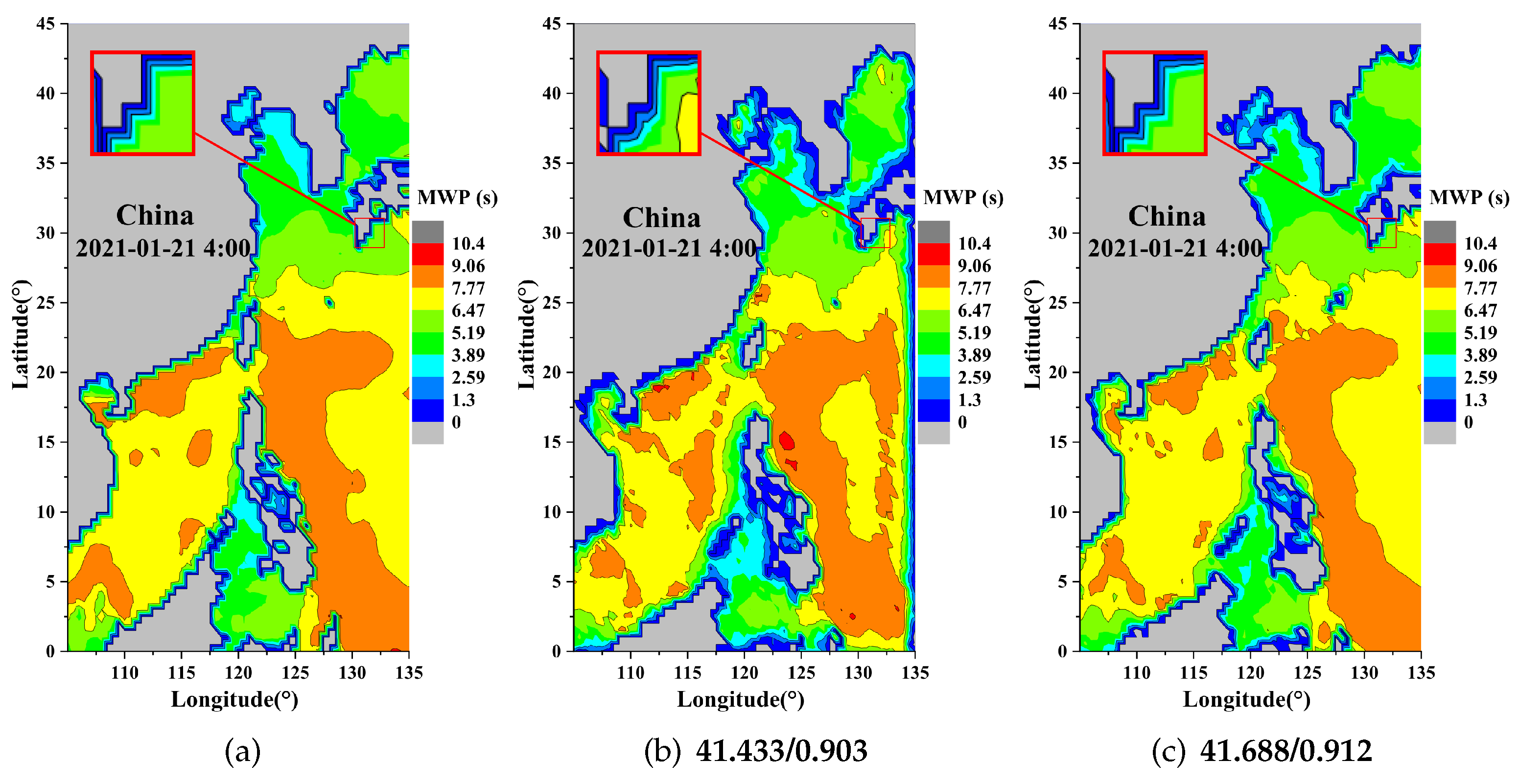
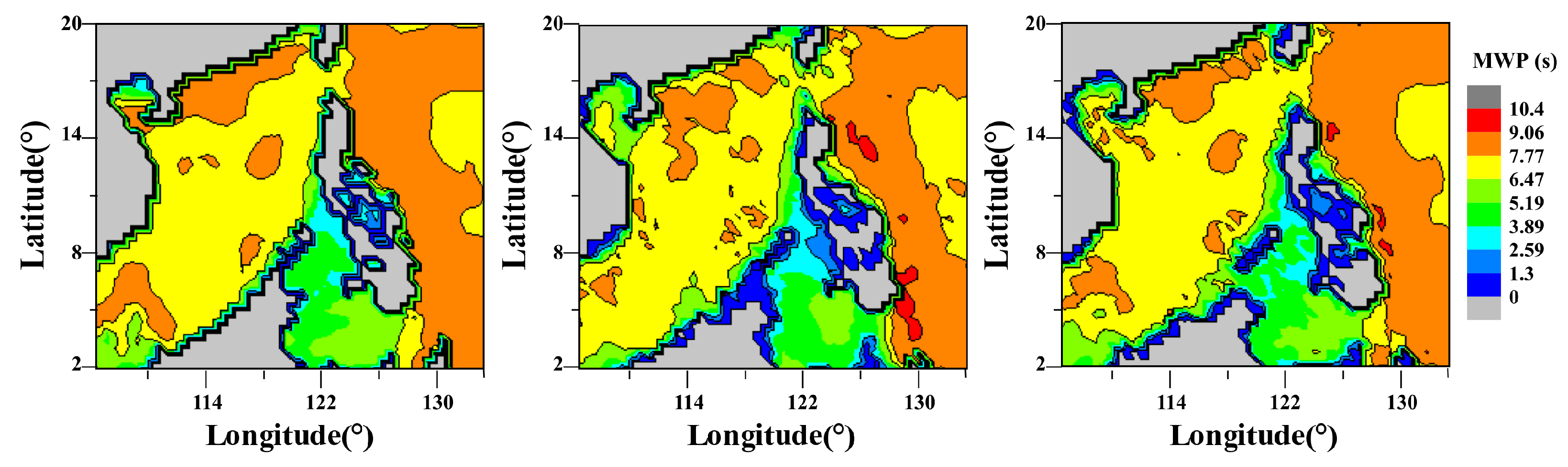
From Figure 17 and Figure 18, it is evident that our method accurately reconstructs the edge distribution of the data, while the interpolation method loses many details. When the high-resolution scale is 2×, at the time point of 2021-01-21 4:00, our method achieves a PSNR of 42.254 and an SSIM of 0.913. When the high-resolution scale is 4×, at the time point of 2021-01-21 4:00, our method achieves a PSNR of 41.688 and an SSIM of 0.912. It can be observed that each method reconstructs parts that do not exist in the original data. This could be attributed to the insufficient accuracy of the feature extraction part of the model in capturing the distribution characteristics of the data.
Based on Table 4 and Figure 11, Figure 12, Figure 13, Figure 14, Figure 15, Figure 16, Figure 17 and Figure 18, it is evident that our method outperforms interpolation methods in terms of its effectiveness and consistency. Overall, the 2× high-resolution reconstruction yields the best results. Specifically, for WS, when increasing the resolution from 0.5° to 0.25°, our method achieves a PSNR value of 49.598 and an SSIM value of 0.981, while the highest PSNR and SSIM values among traditional interpolation methods were 38.453 and 0.711, respectively. For other parameters, although the performance may not be as good as that of WS, our method still achieves the best results. For SWH, when increasing the resolution from 1° to 0.5°, our method achieves a PSNR value of 46.928 and an SSIM value of 0.957, while the highest PSNR and SSIM values among traditional interpolation methods are 45.798 and 0.948, respectively.
5. Discussion
After conducting initial experiments using traditional methods and simple neural networks, we found that the reconstruction of edge details in the data is consistently poor. The PSNR and SSIM values for all methods are not sufficiently high. As a result, we proposed the incorporation of an attention mechanism into the neural network. Initially, we added a complex attention module to the neural network, but due to the low resolution of data, the reconstruction results were not satisfactory in terms of the PSNR and SSIM values. For WS, our method yields a PSNR of 42.324 and an SSIM of 0.912. We conducted experiments with several different attention module configurations, and ultimately found that using a single HOA module yields the best experimental results. For WS, our method yields a PSNR of 43.375 and an SSIM of 0.926. However, there are still some shortcomings in the edge regions. We conducted the experiment with only one GAM module and the results are worse than the models with only one HOA module or HOA module. The GAM module is more effective in enhancing attention to certain parts while suppressing attention to other parts, while the HOA module focuses more on capturing subtle details. Therefore, we introduced the GAM module into the feature extraction part of the model to focus on details and the HOA module into the feature refinement part to refine the detail part. Additionally, we extracted the edge regions of the data prior to the experiments and employed a HOA module to refine the features, combining the final results to obtain the optimal outcome.
Based on satellite observations of WS, SWH, MWP, and MWD, we conducted high-resolution reconstruction experiments. After comparing the processed results, our method consistently outperforms traditional methods. In terms of visual results, our method still demonstrates significant improvements. The figure below shows a comparison of the reconstruction of data, where our method accurately reconstructs many detailed parts.
From Figure 19, Figure 20, Figure 21 and Figure 22, it is evident that our proposed method outperforms the traditional method in many aspects of detail reconstruction. The traditional methods often lack certain details or deviate significantly from the original data distribution. In contrast, our method accurately reconstructs many fine-grained details.
From the comparison of the results in Section 4.2, we can see that although our results are generally better than those of traditional methods, there are still some inaccuracies in the reconstructed results in certain edge regions. This could be attributed to the attention module in the feature refinement part, which may not accurately capture subtle variations in the data features, resulting in insufficient accuracy in refining the features.
Due to the distribution characteristics of certain data, the model was not able to accurately extract and refine features during training, resulting in less satisfactory reconstruction results. In the case of MWP, shown in the Figure 23, neither the traditional interpolation methods nor our proposed method were able to reconstruct certain detailed parts. During the reconstruction process, each method introduced to some extent missing parts that were not present in the original data. This can have an impact on the subsequent analysis of sea clutter characteristics and ocean environmental observations.
The research on the distribution characteristics of the data themselves may not be sufficient, and the model does not extract enough features during feature extraction, which leads to inaccurate feature refinement. The attention module in the feature refinement part may not be the most optimal. From the experimental results in Section 3.6, we can observe that for the data used in this study, a more complex attention module does not necessarily lead to better performance. Therefore, in further research, we can improve and expand our model in the following aspects:
- (1)
- More marine environmental parameters and data sources can be combined to conduct further feature analysis of the data, achieving more comprehensive and multidimensional reconstruction results;
- (2)
- Enhancement of attention modules to enhance the extraction and refinement of important fine-grained features;
- (3)
- Optimization and improvement of network architecture can be studied to enhance reconstruction accuracy and efficiency.
6. Conclusions
In this paper, we employed a global attention mechanism (GAM) module to expand input features in spatial and channel dimensions, and utilized a high-order attention (HOA) module for additional feature learning. The entire network structure is connected using weighted channel concatenation (WCC) technology. To evaluate the proposed method, three metrics are employed: the mean square error (MSE), the peak signal-to-noise ratio (PSNR), and the structural similarity index measure (SSIM). High-resolution reconstructions of the data provided by the European Center for Mesoscale Weather Forecasting are conducted to validate the effectiveness of the proposed method. The results demonstrate that our method achieves notable success in the high-resolution reconstruction of ocean environmental parameters. From Table 4, it can be observed that the proposed method exhibits the highest PSNR and SSIM values among all the reconstructed parameters.
In the future, we will combine traditional methods to further improve our model, modify the network structure to improve the accuracy and precision of the high-resolution reconstruction of the edge detail parts of marine environmental parameters. This will contribute to the study of sea clutter characteristics and provide crucial technical support for achieving offshore target detection and recognition tasks in more complex scenarios.
Author Contributions
Conceptualization, Y.H. and L.M.; funding acquisition, L.M.; methodology, Y.H.; project administration, Y.Z. and J.Z.; resources, L.M. and X.Z.; supervision, L.M. and Z.W.; validation, Y.H.; visualization, Y.H.; writing—original draft preparation, Y.H.; writing—review and editing, L.M., Z.W. and J.W. All authors have read and agreed to the published version of the manuscript.
Funding
This research was funded by National Natural Science Foundation of China (Grant No. 62101297,61901335,62101445 and 62005205), and the Foundation of the National Key Laboratory of the Electromagnetic Environment of China Electronics Tech-nology Group Corporation (Grant No. 202102007), and Natural Science Foundation of Shaanxi Province, China (Grant No. 2020JQ-843, 2020JQ-329 and 2020JQ-843).
Data Availability Statement
Not applicable.
Acknowledgments
Thanks are due for the Marine environment data provided by ECMWF.
Conflicts of Interest
The authors declare no conflict of interest.
References
- Xingwei, J.L.; Lin, M.; Jia, Y. Past, Present and Future Marine Microwave Satellite Missions in China. Remote Sens. 2022, 14, 1330. [Google Scholar]
- Meng, L.; Yan, C.; Zhuang, W.; Zhang, W.; Geng, X.; Yan, X.-H. Reconstructing High-Resolution Ocean Subsurface and Interior Temperature and Salinity Anomalies From Satellite Observations. IEEE Trans. Geosci. Remote Sens. 2022, 60, 1–14. [Google Scholar] [CrossRef]
- Biswas, S.; Sinha, M. Performances of Deep Learning Models for Indian Ocean Wind Speed Prediction. Model. Earth Syst. Environ. 2021, 7, 809–831. [Google Scholar] [CrossRef]
- Luo, Z.; Li, Z.; Zhang, C.; Deng, J.; Qin, T. Low Observable Radar Target Detection Method within Sea Clutter Based on Correlation Estimation. Remote Sens. 2022, 14, 2233. [Google Scholar] [CrossRef]
- Reddy, G.T.; Priya, R.; Parimala, M.; Chowdhary, C.L.; Reddy, M.S.K.; Hakak, S.; Khan, W.Z. A Deep Neural Networks Based Model for Uninterrupted Marine Environment Monitoring. Comput. Commun. 2020, 157, 64–75. [Google Scholar]
- Ma, L.; Wu, J.; Zhang, J.; Wu, Z.; Jeon, G.; Zhang, Y.; Wu, T. Research on Sea Clutter Reflectivity Using Deep Learning Model in Industry 4.0. IEEE Trans. Ind. Inform. 2020, 16, 5929–5937. [Google Scholar] [CrossRef]
- Hao, D.; Ningbo, L.I.U.; Yunlong, D.; Xiaolong, C.; Jian, G. Overview and Prospects of Radar Sea Clutter Measurement Experiments. J. Radars 2019, 8, 281–302. [Google Scholar]
- Klemas, V.; Yan, X.-H. Subsurface and Deeper Ocean Remote Sensing from Satellites: An Overview and New Results. Prog. Oceanogr. 2014, 122, 1–9. [Google Scholar] [CrossRef]
- Cruz, H.; Véstias, M.; Monteiro, J.; Neto, H.; Duarte, R.P. A Review of Synthetic-Aperture Radar Image Formation Algorithms and Implementations: A Computational Perspective. Remote Sens. 2022, 14, 1258. [Google Scholar] [CrossRef]
- Woods, A. Medium-Range Weather Prediction, 1st ed.; Springer: New York, NY, USA, 2005; pp. 23–47. [Google Scholar]
- Linghu, L.; Wu, J.; Wu, Z.; Jeon, G.; Wang, X. GPU-Accelerated Computation of Time-Evolving Electromagnetic Backscattering Field From Large Dynamic Sea Surfaces. IEEE Trans. Ind. Inform. 2020, 16, 3187–3197. [Google Scholar] [CrossRef]
- Linghu, L.; Wu, J.; Wu, Z.; Jeon, G.; Wu, T. GPU-Accelerated Computation of EM Scattering of a Time-Evolving Oceanic Surface Model II: EM Scattering of Actual Oceanic Surface. Remote Sens. 2022, 14, 2727. [Google Scholar] [CrossRef]
- Bounaceur, H.; Khenchaf, A.; Le Caillec, J.-M. Analysis of Small Sea-Surface Targets Detection Performance According to Airborne Radar Parameters in Abnormal Weather Environments. Sensors 2022, 22, 3263. [Google Scholar] [CrossRef] [PubMed]
- Xing, Y.; Song, Q.; Cheng, G. Benefit of Interpolation in Nearest Neighbor Algorithms. SIAM J. Math. Data Sci. 2022, 4, 935–956. [Google Scholar] [CrossRef]
- Meijering, E. A Chronology of Interpolation: From Ancient Astronomy to Modern Signal and Image Processing. Proc. IEEE 2002, 90, 319–342. [Google Scholar] [CrossRef]
- Redondi, A.E.C. Radio Map Interpolation Using Graph Signal Processing. IEEE Commun. Lett. 2018, 22, 153–156. [Google Scholar] [CrossRef] [Green Version]
- Yongchun, L.; Qiang, W. New Solution of Cubic Spline Interpolation Function. Pure Math. 2013, 3, 362–367. [Google Scholar]
- Dong, C.; Loy, C.C.; He, K.; Tang, X. Learning a Deep Convolutional Network for Image Super-Resolution. In Proceedings of the Computer Vision—ECCV, Zurich, Switzerland, 6–12 September 2014; pp. 184–199. [Google Scholar]
- Kim, J.; Lee, J.K.; Lee, K.M. Accurate Image Super-Resolution Using Very Deep Convolutional Networks. In Proceedings of the 2016 IEEE Conference on Computer Vision and Pattern Recognition (CVPR), Las Vegas, NV, USA, 27–30 June 2016; pp. 1646–1654. [Google Scholar]
- Lim, B.; Son, S.; Kim, H.; Nah, S.; Lee, K.M. Enhanced Deep Residual Networks for Single Image Super-Resolution. In Proceedings of the 2017 IEEE Conference on Computer Vision and Pattern Recognition Workshops (CVPRW), Honolulu, HI, USA, 21–26 July 2017; pp. 1132–1140. [Google Scholar]
- Li, J.; Fang, F.; Li, J.; Mei, K.; Zhang, G. MDCN: Multi-Scale Dense Cross Network for Image Super-Resolution. IEEE Trans. Circuits Syst. Video Technol. 2021, 31, 2547–2561. [Google Scholar] [CrossRef]
- Ducournau, A.; Fablet, R. Deep Learning for Ocean Remote Sensing: An Application of Convolutional Neural Networks for Super-Resolution on Satellite-Derived SST Data. In Proceedings of the 2016 9th IAPR Workshop on Pattern Recogniton in Remote Sensing (PRRS), Cancun, Mexico, 4 December 2016; pp. 1–6. [Google Scholar]
- Wang, Z.; Wang, G.; Guo, X.; Hu, J.; Dai, M. Reconstruction of High-Resolution Sea Surface Salinity over 2003–2020 in the South China Sea Using the Machine Learning Algorithm LightGBM Model. Remote Sens. 2022, 14, 6147. [Google Scholar] [CrossRef]
- Su, H.; Wang, A.; Zhang, T.; Qin, T.; Du, X.; Yan, X.-H. Super-Resolution of Subsurface Temperature Field from Remote Sensing Observations Based on Machine Learning. Int. J. Appl. Earth Obs. Geoinf. 2021, 102, 102440. [Google Scholar] [CrossRef]
- Gao, L.; Li, X.; Song, J.; Shen, H.T. Hierarchical LSTMs with Adaptive Attention for Visual Captioning. IEEE Trans. Pattern Anal. Mach. Intell. 2020, 42, 1112–1131. [Google Scholar] [CrossRef] [Green Version]
- Fu, J.; Liu, J.; Tian, H.; Li, Y.; Bao, Y.; Fang, Z.; Lu, H. Dual Attention Network for Scene Segmentation. In Proceedings of the 2019 IEEE/CVF Conference on Computer Vision and Pattern Recognition (CVPR), Long Beach, CA, USA, 15–20 June 2019; pp. 3141–3149. [Google Scholar]
- Zhong, Z.; Lin, Z.; Bidart, R.; Hu, X.; Ben Daya, I.; Li, Z.; Zheng, W.-S.; Li, J.; Wong, A. Squeeze-and-Attention Networks for Semantic Segmentation. In Proceedings of the IEEE/CVF Conference on Computer Vision and Pattern Recognition, Seattle, WA, USA, 14–19 June 2020; pp. 13065–13074. [Google Scholar]
- Luong, T.; Pham, H.; Manning, C.D. Effective Approaches to Attention-Based Neural Machine Translation. In Proceedings of the 2015 Conference on Empirical Methods in Natural Language Processing, Lisbon, Portugal, 17–21 September 2015. [Google Scholar]
- Yin, W.; Schütze, H.; Xiang, B.; Zhou, B. ABCNN: Attention-Based Convolutional Neural Network for Modeling Sentence Pairs. Trans. Assoc. Comput. Linguist. 2016, 4, 259–272. [Google Scholar] [CrossRef]
- Serrano, S.; Smith, N.A. Is Attention Interpretable? In Proceedings of the 57th Annual Meeting of the Association for Computational Linguistics, Florence, Italy, 28 July–2 August 2019; pp. 2931–2951. [Google Scholar]
- Chan, W.; Jaitly, N.; Le, Q.; Vinyals, O. Listen, Attend and Spell: A Neural Network for Large Vocabulary Conversational Speech Recognition. In Proceedings of the 2016 IEEE International Conference on Acoustics, Speech and Signal Processing (ICASSP), Shanghai, China, 20–25 March 2016; pp. 4960–4964. [Google Scholar]
- Tran, D.T.; Iosifidis, A.; Kanniainen, J.; Gabbouj, M. Temporal Attention-Augmented Bilinear Network for Financial Time-Series Data Analysis. IEEE Trans. Neural Netw. Learn. Syst. 2019, 30, 1407–1418. [Google Scholar] [CrossRef] [Green Version]
- Chaudhari, S.; Mithal, V.; Polatkan, G.; Ramanath, R. An Attentive Survey of Attention Models. ACM Trans. Intell. Syst. Technol. 2021, 12, 1–32. [Google Scholar] [CrossRef]
- Hu, J.; Shen, L.; Sun, G. Squeeze-and-Excitation Networks. In Proceedings of the 2018 IEEE/CVF Conference on Computer Vision and Pattern Recognition, Salt Lake City, UT, USA, 18–23 June 2018; pp. 7132–7141. [Google Scholar]
- Woo, S.; Park, J.; Lee, J.-Y.; Kweon, I.S. CBAM: Convolutional Block Attention Module. In Proceedings of the Computer Vision—ECCV, Munich, Germany, 8–14 September 2018; pp. 3–19. [Google Scholar]
- Misra, D.; Nalamada, T.; Arasanipalai, A.U.; Hou, Q. Rotate to Attend: Convolutional Triplet Attention Module. In Proceedings of the 2021 IEEE Winter Conference on Applications of Computer Vision (WACV), Virtual, 3–8 January 2021; pp. 3138–3147. [Google Scholar]
- Liu, Y.; Shao, Z.; Hoffmann, N. Global Attention Mechanism: Retain Information to Enhance Channel-Spatial Interactions. arXiv 2021, arXiv:2112.05561. [Google Scholar]
- Chen, B.; Deng, W.; Hu, J. Mixed High-Order Attention Network for Person Re-Identification. In Proceedings of the IEEE/CVF International Conference on Computer Vision, Seoul, Republic of Korea, 27 October–2 November 2019; pp. 371–381. [Google Scholar]
- Zhang, Y.; Li, K.; Li, K.; Wang, L.; Zhong, B.; Fu, Y. Image Super-Resolution Using Very Deep Residual Channel Attention Networks. In Proceedings of the European Conference on Computer Vision, Munich, Germany, 8–14 September 2018; pp. 286–301. [Google Scholar]
- Park, J.; Woo, S.; Lee, J.-Y.; Kweon, I.S. BAM: Bottleneck Attention Module. In Proceedings of the British Machine Vision Conference, Newcastle, UK, 3–6 September 2018. [Google Scholar]
- Zhang, X.; Zhou, X.; Lin, M.; Sun, J. ShuffleNet: An Extremely Efficient Convolutional Neural Network for Mobile Devices. In Proceedings of the IEEE Conference on Computer Vision and Pattern Recognition, Salt Lake City, UT, USA, 18–22 June 2018; pp. 6848–6856. [Google Scholar]
- Hu, Y.; Li, J.; Huang, Y.; Gao, X. Channel-Wise and Spatial Feature Modulation Network for Single Image Super-Resolution. IEEE Trans. Circuits Syst. Video Technol. 2018, 30, 3911–3927. [Google Scholar] [CrossRef] [Green Version]
- Kingma, D.P.; Ba, J. Adam: A Method for Stochastic Optimization. In Proceedings of the 3rd International Conference on Learning Representations, San Diego, CA, USA, 7–9 May 2015. [Google Scholar]
- Picking Loss Functions—A Comparison between MSE, Cross Entropy, and Hinge Loss. Available online: https://rohanvarma.me/Loss-Functions/ (accessed on 14 May 2023).
- Differences between L1 and L2 as Loss Function and Regularization. Available online: http://www.chioka.in/differences-between-l1-and-l2-as-loss-function-and-regularization/ (accessed on 14 May 2023).
- Girshick, R. Fast R-CNN. In Proceedings of the 2015 IEEE International Conference on Computer Vision (ICCV), Santiago, Chile, 7–13 December 2015; pp. 1440–1448. [Google Scholar]
- James, G.; Witten, D.; Hastie, T.; Tibshirani, R. (Eds.) Linear Model Selection and Regularization. In An Introduction to Statistical Learning: With Applications in R; Springer Texts in Statistics; Springer: New York, NY, USA, 2013; pp. 203–264. [Google Scholar]
- Erfurt, J.; Helmrich, C.R.; Bosse, S.; Schwarz, H.; Marpe, D.; Wiegand, T. A Study of the Perceptually Weighted Peak Signal-To-Noise Ratio (WPSNR) for Image Compression. In Proceedings of the 2019 IEEE International Conference on Image Processing (ICIP), Taipei, Taiwan, 22–25 September 2019; pp. 2339–2343. [Google Scholar]
- Wang, Z.; Bovik, A.C.; Sheikh, H.R.; Simoncelli, E.P. Image Quality Assessment: From Error Visibility to Structural Similarity. IEEE Trans. Image Process. 2004, 13, 600–612. [Google Scholar] [CrossRef] [Green Version]
Figure 1.
Overview of the proposed network.

Figure 2.
Overview of GAM module.

Figure 3.
Channel attention module.

Figure 4.
Spatial attention module.

Figure 5.
Illustration of HOA modules in the case of R = 1.

Figure 6.
Illustration of HOA modules in the case of R = 3.

Figure 7.
The convergence effect of different loss functions. (a) The high-resolution scale factor is 2×. (b) The high-resolution scale factor is 4×.
Figure 7.
The convergence effect of different loss functions. (a) The high-resolution scale factor is 2×. (b) The high-resolution scale factor is 4×.

Figure 8.
The mean MSE value of different interpolation methods. (a) The high-resolution scale is 2×. (b) The high-resolution scale is 4×.
Figure 8.
The mean MSE value of different interpolation methods. (a) The high-resolution scale is 2×. (b) The high-resolution scale is 4×.

Figure 9.
The mean MSE of our method. (a) The high-resolution scale is 2×. (b) The high-resolution scale is 4×.
Figure 9.
The mean MSE of our method. (a) The high-resolution scale is 2×. (b) The high-resolution scale is 4×.

Figure 10.
The mean MSE values of traditional method. (a) The high-resolution scale is 2×. (b) The high-resolution scale is 4×.
Figure 10.
The mean MSE values of traditional method. (a) The high-resolution scale is 2×. (b) The high-resolution scale is 4×.

Figure 11.
Comparison of enlarged image details in a specific region of the reconstructed WS data. The high-resolution scale is 2×. The two values are, respectively, PSNR/SSIM. (a) Original data. (b) Interpolation method (c) Our method.
Figure 11.
Comparison of enlarged image details in a specific region of the reconstructed WS data. The high-resolution scale is 2×. The two values are, respectively, PSNR/SSIM. (a) Original data. (b) Interpolation method (c) Our method.

Figure 12.
Comparison of enlarged image details in a specific region of the reconstructed WS data. The high-resolution scale is 4×. The two values are, respectively, PSNR/SSIM. (a) Original. (b) Interpolation method (c) Our method.
Figure 12.
Comparison of enlarged image details in a specific region of the reconstructed WS data. The high-resolution scale is 4×. The two values are, respectively, PSNR/SSIM. (a) Original. (b) Interpolation method (c) Our method.

Figure 13.
Comparison of enlarged image details in a specific region of the reconstructed SWH data. The high-resolution scale is 2×. The two values are, respectively, PSNR/SSIM. (a) Original data. (b) Interpolation method (c) Our method.
Figure 13.
Comparison of enlarged image details in a specific region of the reconstructed SWH data. The high-resolution scale is 2×. The two values are, respectively, PSNR/SSIM. (a) Original data. (b) Interpolation method (c) Our method.

Figure 14.
Comparison of enlarged image details in a specific region of the reconstructed SWH data. The high-resolution scale is 4×. The two values are, respectively, PSNR/SSIM. (a) Original data. (b) Interpolation method (c) Our method.
Figure 14.
Comparison of enlarged image details in a specific region of the reconstructed SWH data. The high-resolution scale is 4×. The two values are, respectively, PSNR/SSIM. (a) Original data. (b) Interpolation method (c) Our method.

Figure 15.
Comparison of enlarged image details in a specific region of the reconstructed MWD data. The high-resolution scale is 2×. The two values are, respectively, PSNR/SSIM. (a) Original data. (b) Interpolation method (c) Our method.
Figure 15.
Comparison of enlarged image details in a specific region of the reconstructed MWD data. The high-resolution scale is 2×. The two values are, respectively, PSNR/SSIM. (a) Original data. (b) Interpolation method (c) Our method.

Figure 16.
Comparison of enlarged image details in a specific region of the reconstructed MWD data. The high-resolution scale is 4×. The two values are, respectively, PSNR/SSIM. (a) Original data. (b) Interpolation method (c) Our method.
Figure 16.
Comparison of enlarged image details in a specific region of the reconstructed MWD data. The high-resolution scale is 4×. The two values are, respectively, PSNR/SSIM. (a) Original data. (b) Interpolation method (c) Our method.

Figure 17.
Comparison of enlarged image details in a specific region of the reconstructed MWP data. The high-resolution scale is 2×. The two values are, respectively, PSNR/SSIM. (a) Original data. (b) Interpolation method (c) Our method.
Figure 17.
Comparison of enlarged image details in a specific region of the reconstructed MWP data. The high-resolution scale is 2×. The two values are, respectively, PSNR/SSIM. (a) Original data. (b) Interpolation method (c) Our method.

Figure 18.
Comparison of enlarged image details in a specific region of the reconstructed MWP data. The high-resolution scale is 4×. The two values are, respectively, PSNR/SSIM. (a) Original data. (b) Interpolation method (c) Our method.
Figure 18.
Comparison of enlarged image details in a specific region of the reconstructed MWP data. The high-resolution scale is 4×. The two values are, respectively, PSNR/SSIM. (a) Original data. (b) Interpolation method (c) Our method.

Figure 19.
Comparison of some details of WS. From left to right, the images represent the original image, the traditional method and our method. (a,b) represent the comparison of different details.
Figure 19.
Comparison of some details of WS. From left to right, the images represent the original image, the traditional method and our method. (a,b) represent the comparison of different details.

Figure 20.
Comparison of some details of SWH. From left to right, the images represent the original image, the traditional method and our method. (a,b) represent the comparison of different details.
Figure 20.
Comparison of some details of SWH. From left to right, the images represent the original image, the traditional method and our method. (a,b) represent the comparison of different details.

Figure 21.
Comparison of some details of MWD. From left to right, the images represent the original image, the traditional method and our method. (a,b) represent the comparison of different details.
Figure 21.
Comparison of some details of MWD. From left to right, the images represent the original image, the traditional method and our method. (a,b) represent the comparison of different details.

Figure 22.
Comparison of some details of MWP. From left to right, the images represent the original image, the traditional method and our method. (a,b) represent the comparison of different details.
Figure 22.
Comparison of some details of MWP. From left to right, the images represent the original image, the traditional method and our method. (a,b) represent the comparison of different details.

Figure 23.
Comparison of some details of mwp. From left to right, the images represent the original image, the traditional method, and our method.
Figure 23.
Comparison of some details of mwp. From left to right, the images represent the original image, the traditional method, and our method.


Table 1.
Training dataset information.
| Marine Environmental Parameter | Number | Resolution | Data Size |
|---|---|---|---|
| wind | 8186 | 0.25° | |
| swh | 8186 | 0.5° | |
| mwd | 8186 | 0.5° | |
| mwp | 8186 | 0.5° |
Table 2.
Training dataset information after downsampling.
| Marine Environmental Parameter | Number | Resolution | Data Size with a Downsampling Factor of 2 | Data Size with a Downsampling Factor of 4 |
|---|---|---|---|---|
| wind | 8186 | 0.25° | ||
| swh | 8186 | 0.5° | ||
| mwd | 8186 | 0.5° | ||
| mwp | 8186 | 0.5° |
Table 3.
Compare the experimental results with different modules. All models are tested on the same dataset with consistent experimental settings.
Table 3.
Compare the experimental results with different modules. All models are tested on the same dataset with consistent experimental settings.
| Model | MSE | PSNR | SSIM |
|---|---|---|---|
| Baseline model | 4.575 | 41.527 | 0.915 |
| Model with GAM Module | 3.467 | 42.723 | 0.932 |
| to (HOA Modules) | 3.512 | 42.675 | 0.927 |
| to (HOA Modules) | 3.438 | 42.767 | 0.928 |
| (HOA Module) | 3.478 | 42.718 | 0.944 |
| (HOA Module) | 3.268 | 42.988 | 0.947 |
| (HOA Module) | 2.978 | 43.391 | 0.929 |
| Our model (GAM and HOA Module) | 2.299 | 44.515 | 0.934 |
The bold numbers indicates the best performance.
Table 4.
Evaluation results of marine environmental data.
| Data | Scale Factor | Evaluation Criteria | Traditional Method | Our Method | |
|---|---|---|---|---|---|
| Linear Interpolation | Alternate Downsampling | Average Downsampling | |||
| WS | 2× | MSE | 9.285 | 0.713 | 0.734 |
| PSNR | 38.453 | 49.598 | 49.471 | ||
| SSIM | 0.711 | 0.981 | 0.977 | ||
| 4× | MSE | 9.472 | 0.755 | 0.817 | |
| PSNR | 38.367 | 49.362 | 49.015 | ||
| SSIM | 0.703 | 0.961 | 0.957 | ||
| SWH | 2× | MSE | 1.711 | 1.339 | 1.319 |
| PSNR | 45.798 | 46.864 | 46.928 | ||
| SSIM | 0.948 | 0.957 | 0.957 | ||
| 4× | MSE | 2.31 | 1.894 | 1.883 | |
| PSNR | 44.5 | 45.358 | 45.386 | ||
| SSIM | 0.926 | 0.942 | 0.942 | ||
| MWD | 2× | MSE | 3.661 | 3.035 | 3.693 |
| PSNR | 42.501 | 43.309 | 42.457 | ||
| SSIM | 0.910 | 0.930 | 0.921 | ||
| 4× | MSE | 3.798 | 3.715 | 3.222 | |
| PSNR | 42.335 | 42.431 | 43.049 | ||
| SSIM | 0.909 | 0.918 | 0.913 | ||
| MWP | 2× | MSE | 3.862 | 3.162 | 2.299 |
| PSNR | 42.263 | 43.148 | 44.515 | ||
| SSIM | 0.93 | 0.940 | 0.934 | ||
| 4× | MSE | 3.951 | 3.741 | 3.645 | |
| PSNR | 42.172 | 42.401 | 42.513 | ||
| SSIM | 0.939 | 0.936 | 0.944 | ||
The bold numbers indicates the best performance.
Disclaimer/Publisher’s Note: The statements, opinions and data contained in all publications are solely those of the individual author(s) and contributor(s) and not of MDPI and/or the editor(s). MDPI and/or the editor(s) disclaim responsibility for any injury to people or property resulting from any ideas, methods, instructions or products referred to in the content. |
© 2023 by the authors. Licensee MDPI, Basel, Switzerland. This article is an open access article distributed under the terms and conditions of the Creative Commons Attribution (CC BY) license (https://creativecommons.org/licenses/by/4.0/).
Share and Cite
MDPI and ACS Style
Hu, Y.; Ma, L.; Zhang, Y.; Wu, Z.; Wu, J.; Zhang, J.; Zhang, X. Research on High-Resolution Reconstruction of Marine Environmental Parameters Using Deep Learning Model. Remote Sens. 2023, 15, 3419. https://doi.org/10.3390/rs15133419
AMA Style
Hu Y, Ma L, Zhang Y, Wu Z, Wu J, Zhang J, Zhang X. Research on High-Resolution Reconstruction of Marine Environmental Parameters Using Deep Learning Model. Remote Sensing. 2023; 15(13):3419. https://doi.org/10.3390/rs15133419
Chicago/Turabian StyleHu, Yaning, Liwen Ma, Yushi Zhang, Zhensen Wu, Jiaji Wu, Jinpeng Zhang, and Xiaoxiao Zhang. 2023. "Research on High-Resolution Reconstruction of Marine Environmental Parameters Using Deep Learning Model" Remote Sensing 15, no. 13: 3419. https://doi.org/10.3390/rs15133419
Note that from the first issue of 2016, this journal uses article numbers instead of page numbers. See further details here.