
Spatiotemporal Features of the Surface Urban Heat Island of Bacău City (Romania) during the Warm Season and Local Trends of LST Imposed by Land Use Changes during the Last 20 Years
 , and
, and 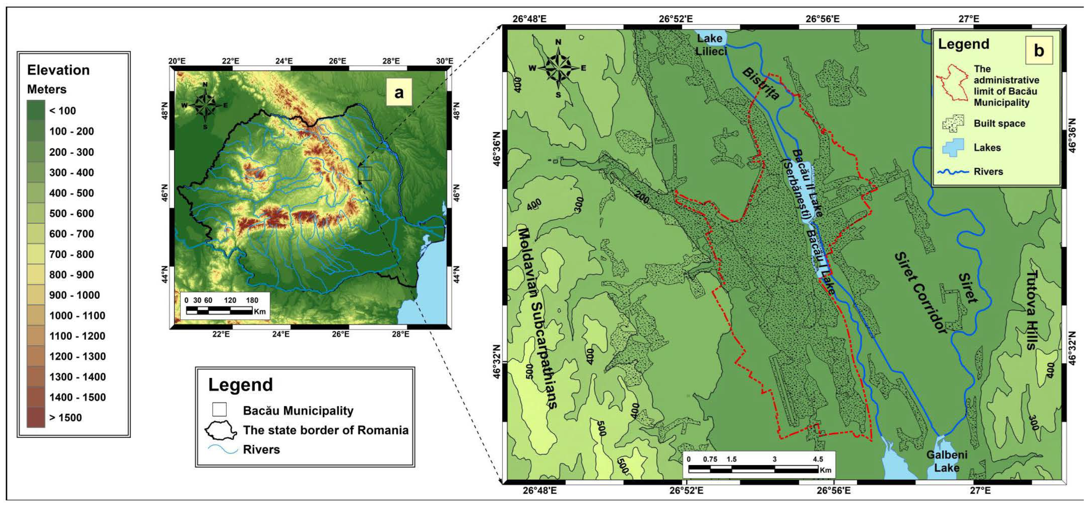
Abstract
:1. Introduction
2. Data and Methodology
2.1. Study Region and Its Main Thermal Conditions
2.2. Data
2.2.1. Land Surface Temperature (LST)
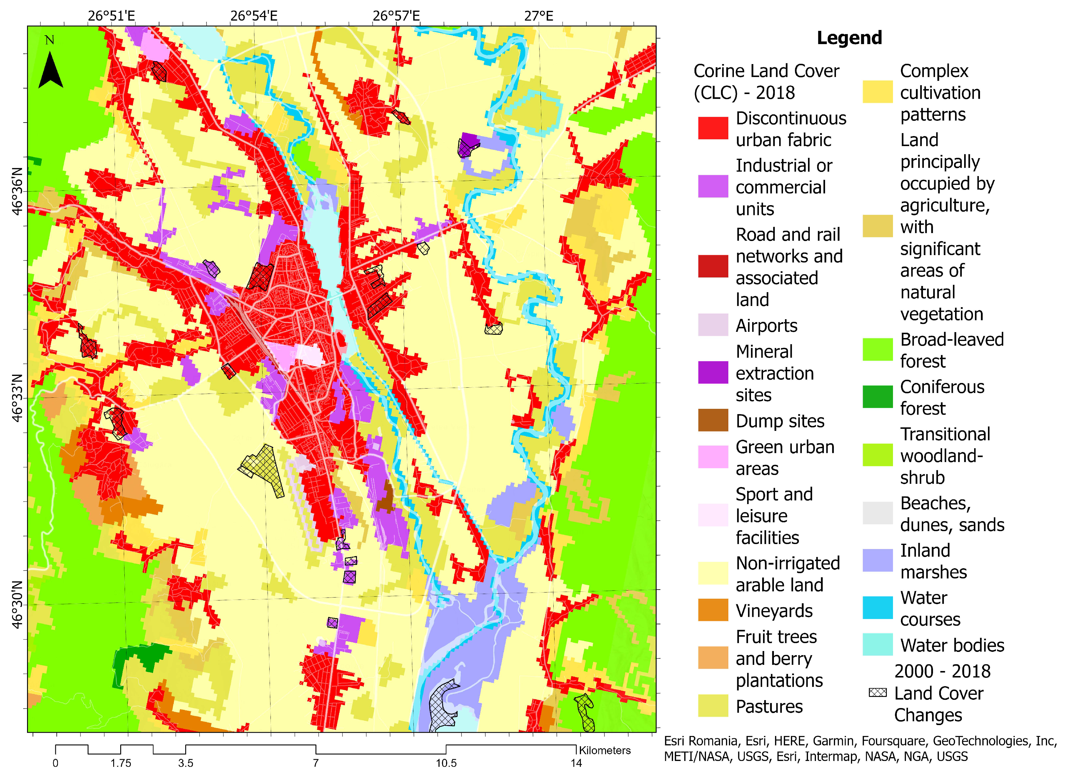
2.2.2. Land Cover Data
2.3. Methodology
2.3.1. Extraction and Treatment of LST Products
2.3.2. Resampling of LST Products at Various Spatial Resolutions
2.3.3. Elaboration of the Grid Point MODIS LST Database
2.3.4. Detrending of LST Data for 2001–2020
3. Results and Discussion
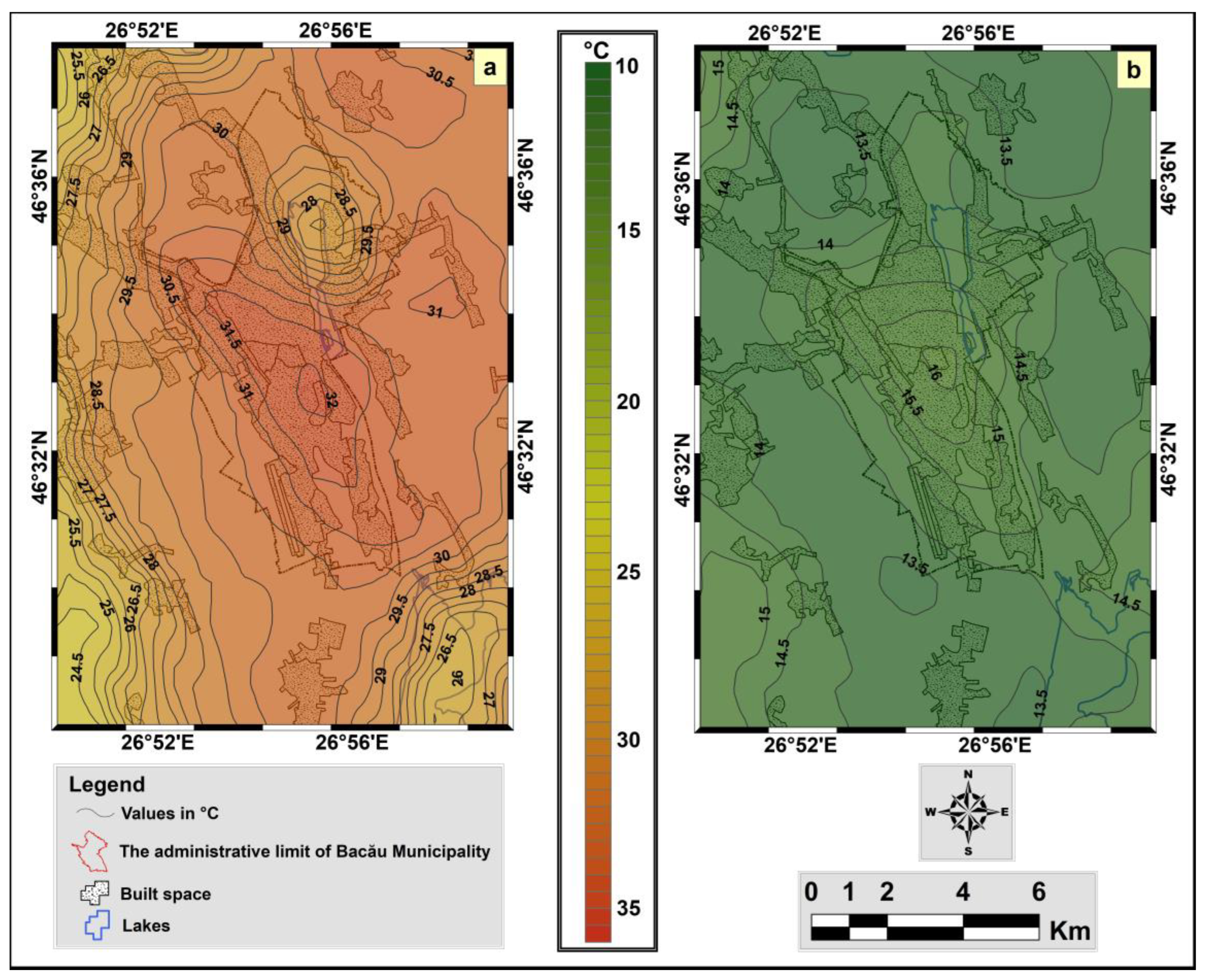
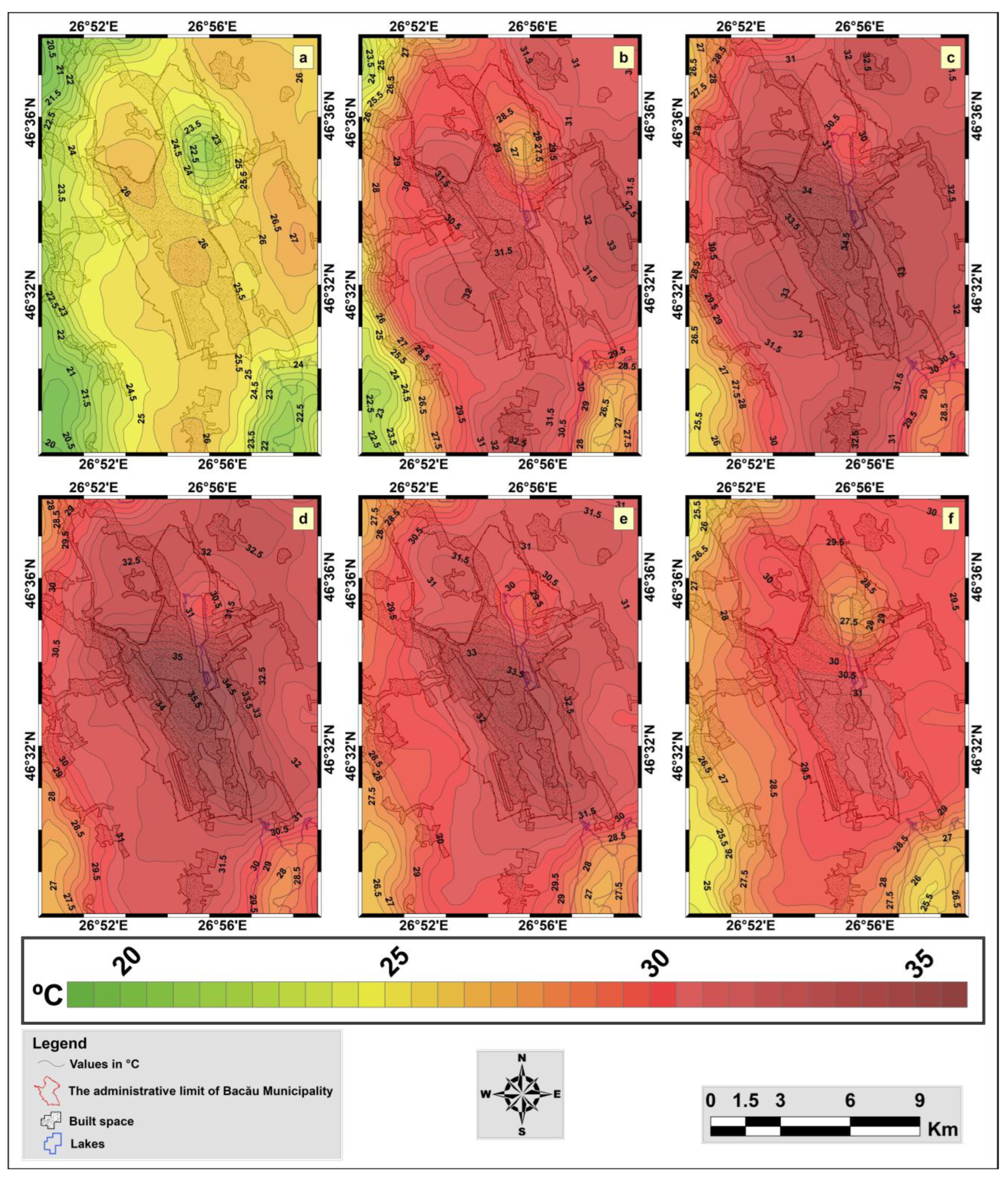
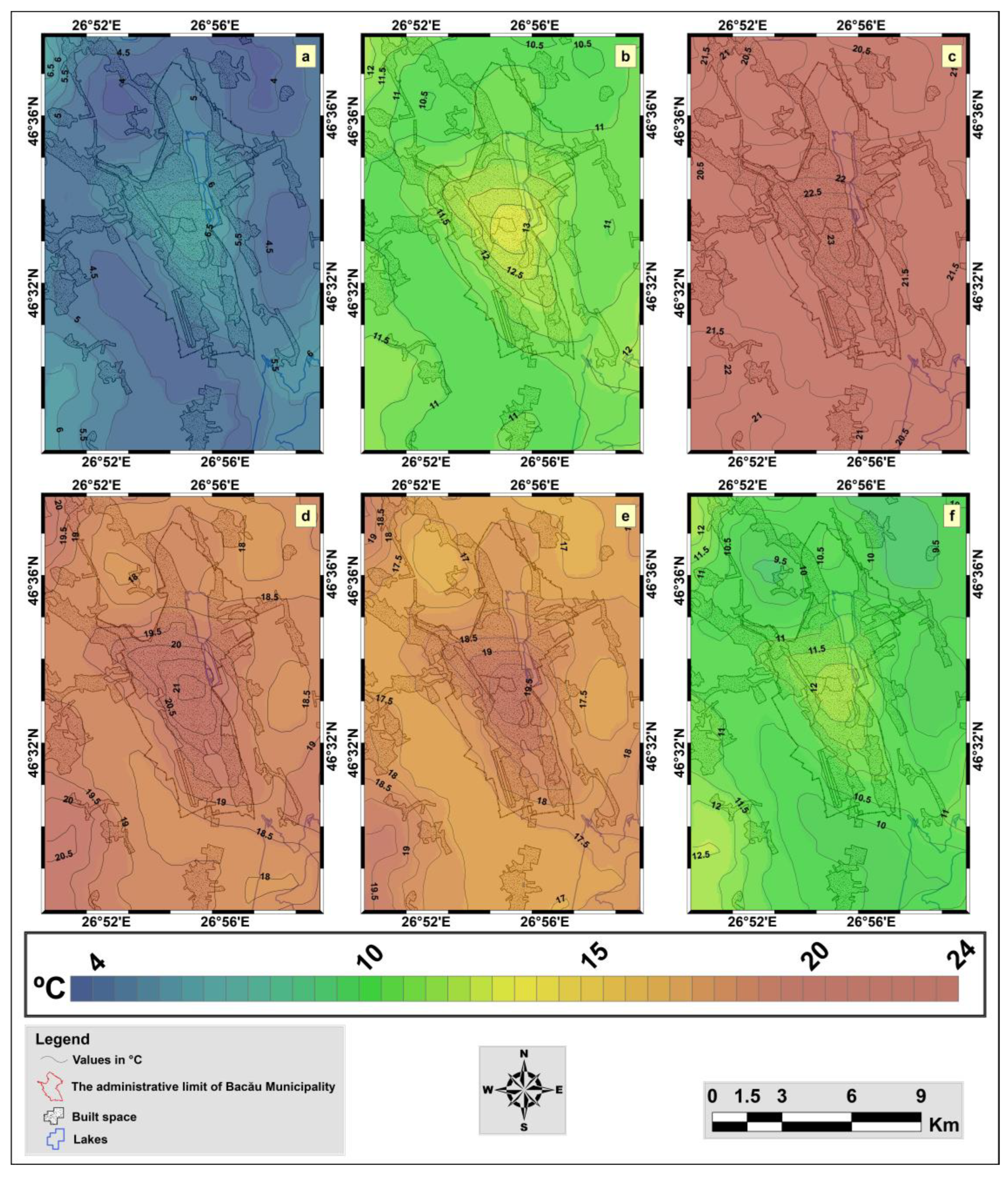
3.1. General Characteristics of the Warm Season SUHI in Bacău City
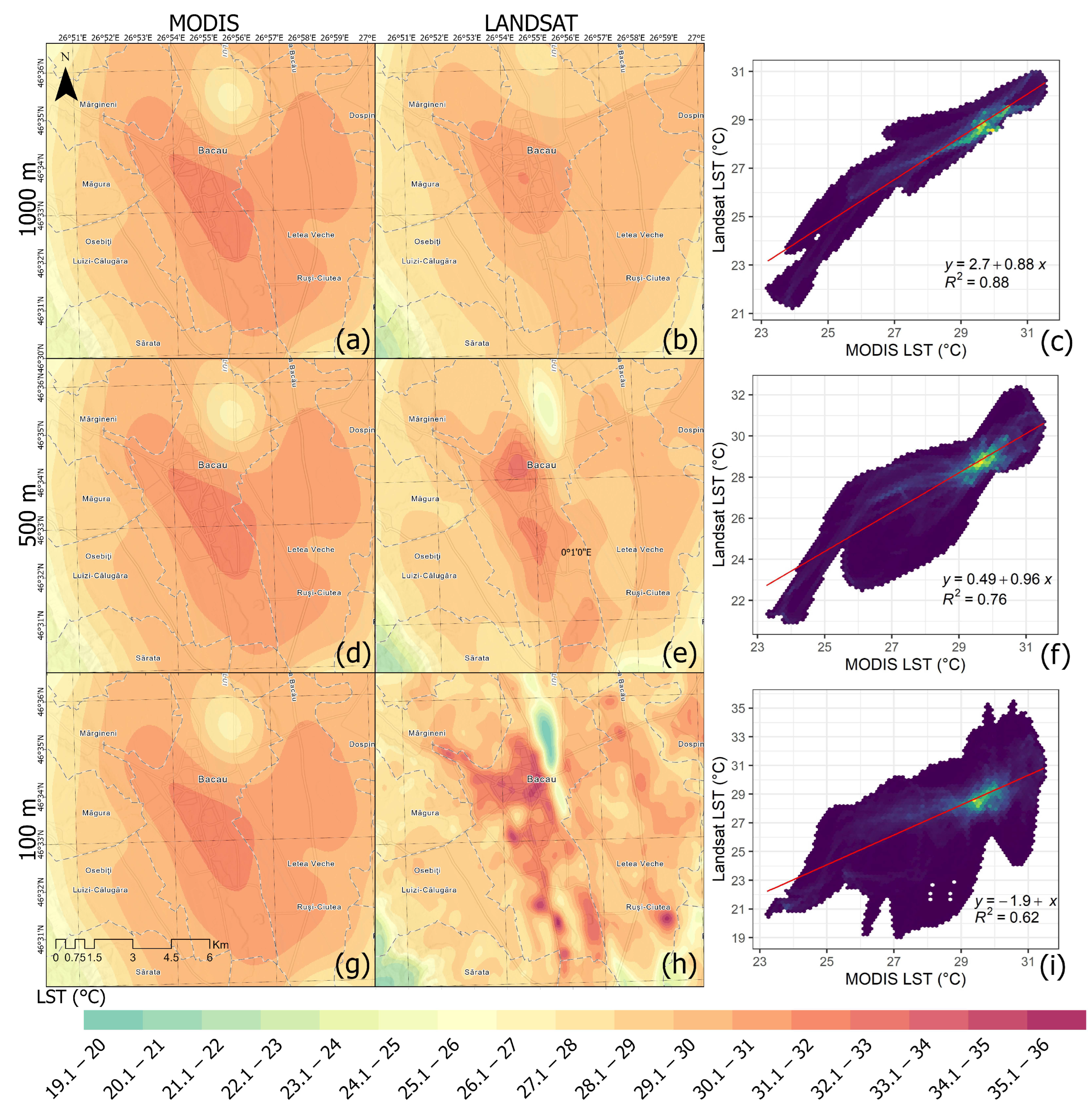
3.2. Comparison between the SUHI Derived from MODIS Terra and Landsat
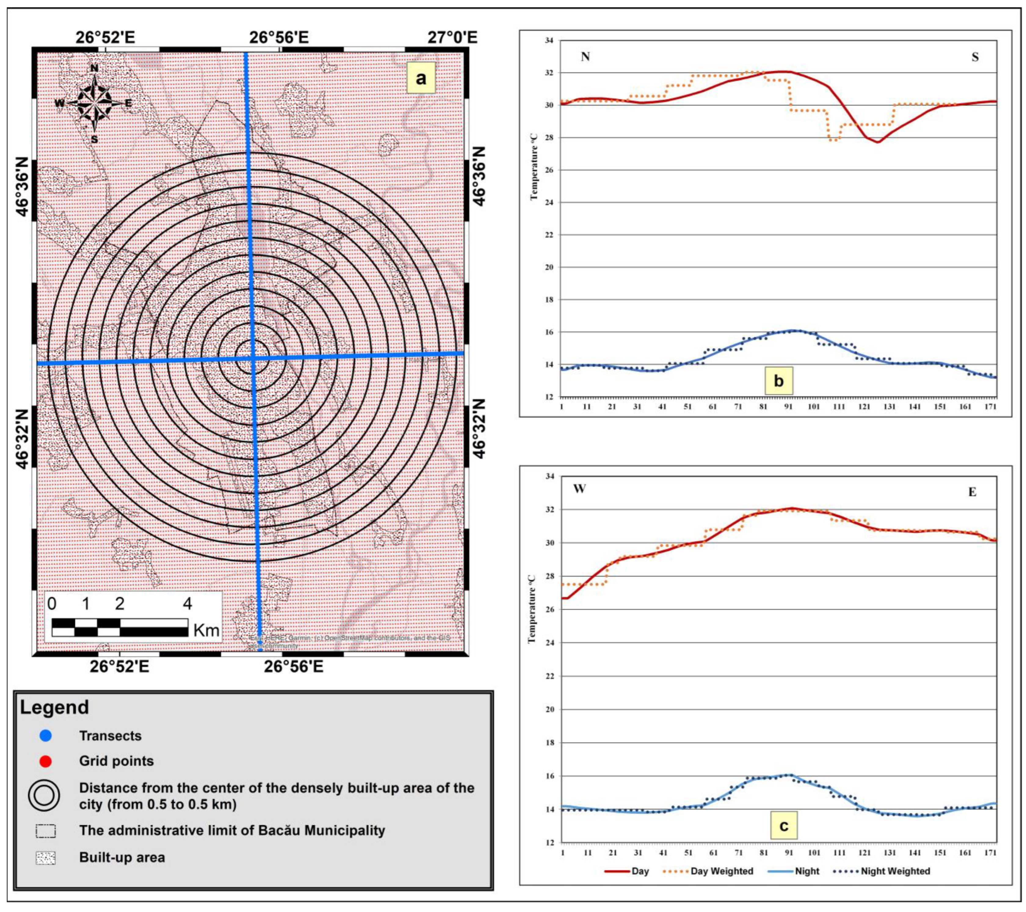
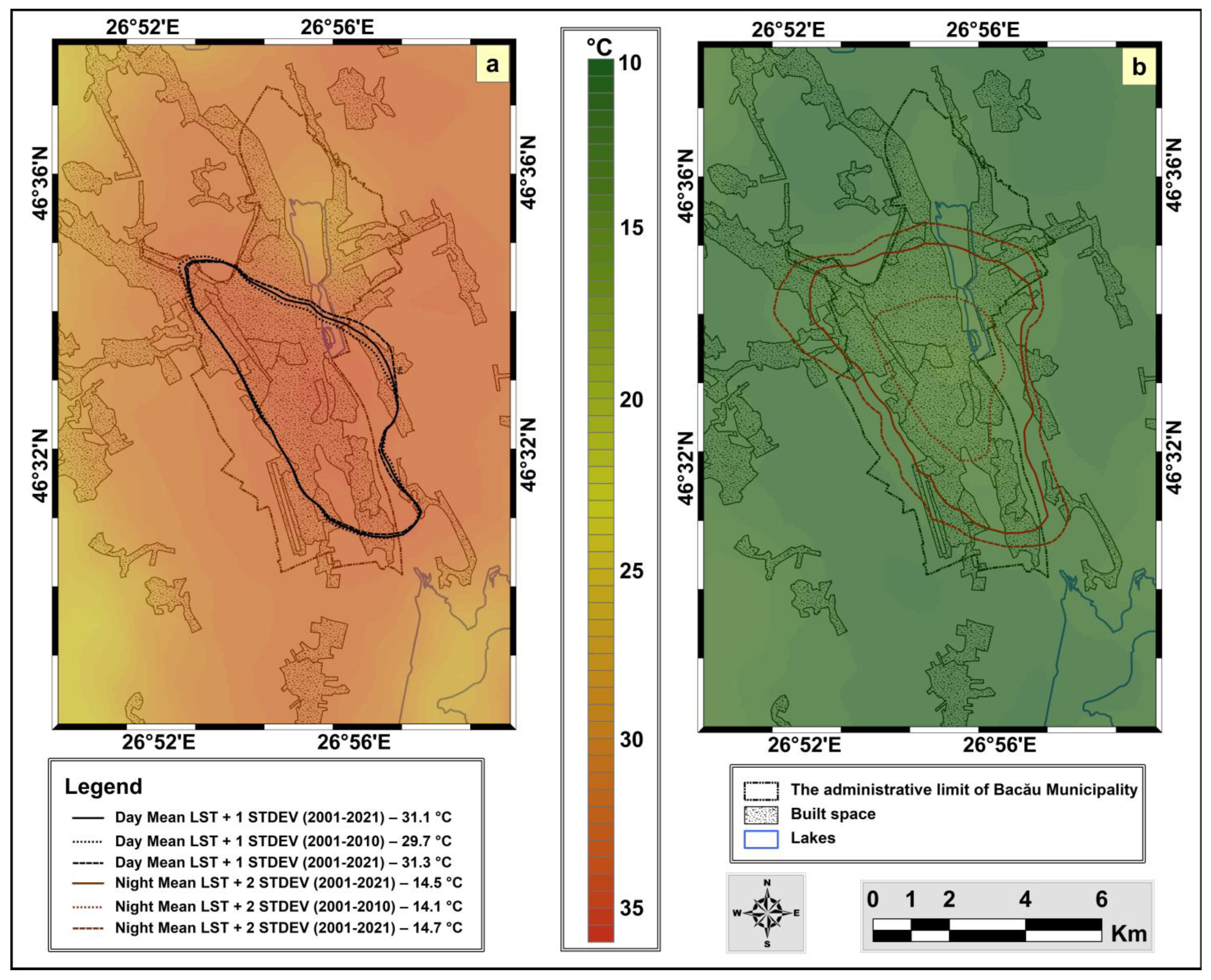
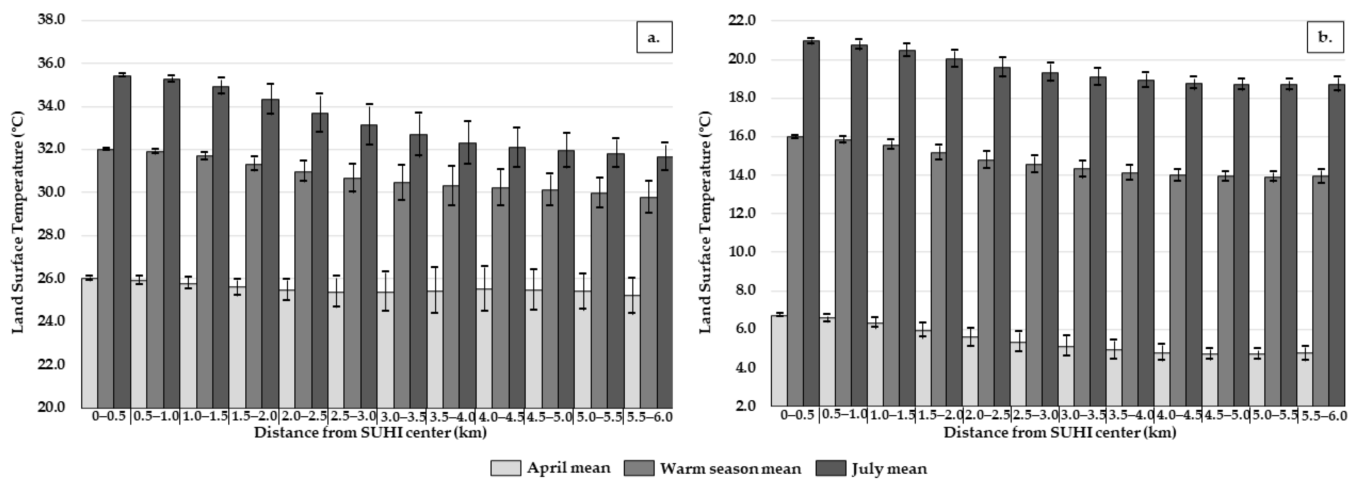
3.3. Limits and Geometry of Bacău City’s SUHI
3.4. SUHI Intensity
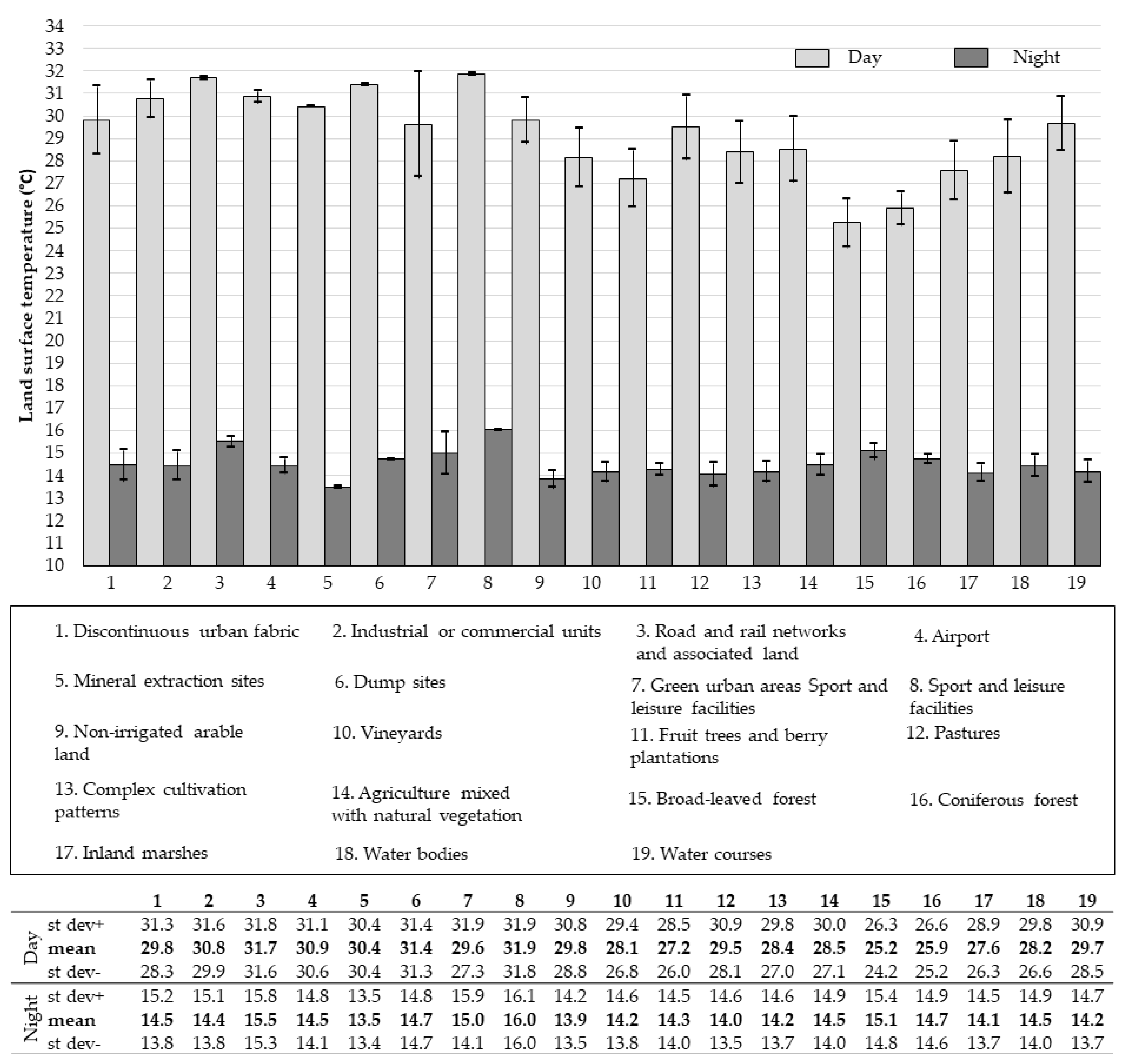
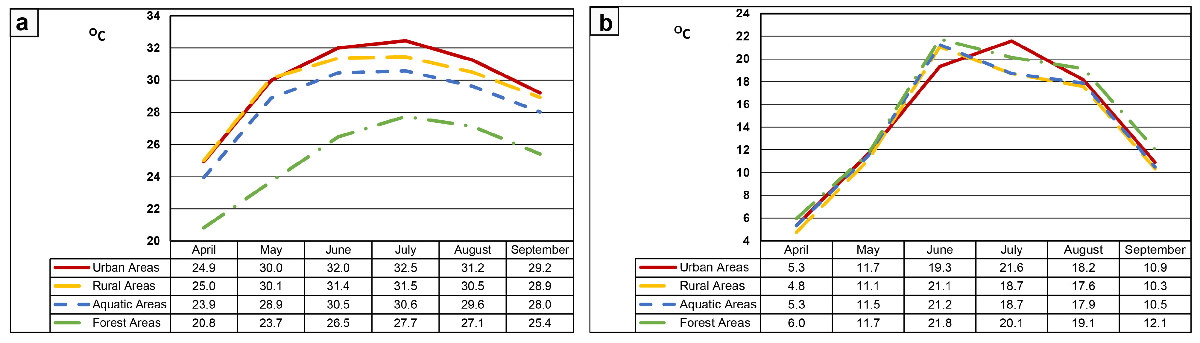
3.5. Influence of Land Use on the SUHI
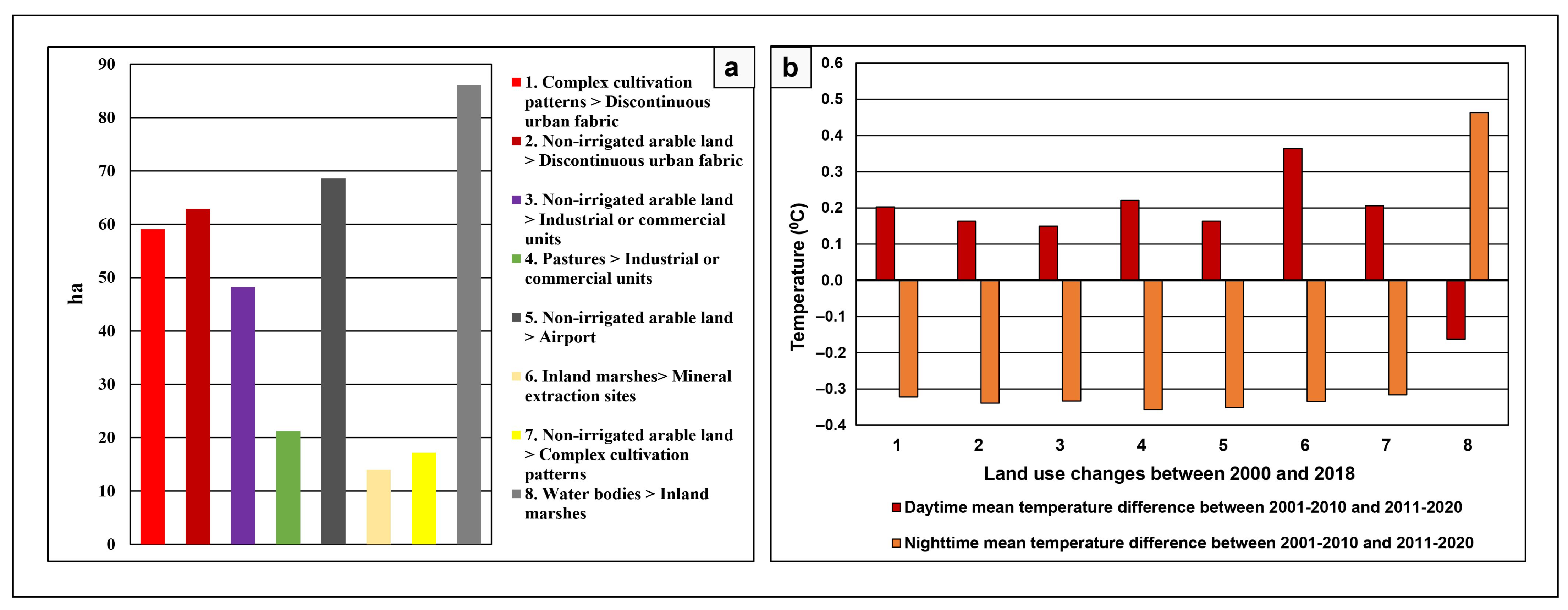
3.6. Land Use Changes and Their Impact on the LST
4. Conclusions
Author Contributions
Funding
Data Availability Statement
Acknowledgments
Conflicts of Interest
References
- Zhou, J.; Li, J.; Yue, J. Analysis of urban heat island (UHI) in the Bejing metropolitan area by time-series MODIS data. In Proceedings of the IEEE International Geoscience and Remote Sensing Symposium, Honolulu, HI, USA, 25–30 July 2010; pp. 3327–3330. [Google Scholar] [CrossRef]
- Zhou, J.; Gurney, K. A new methodology for quantifying on-site residential and commercial fossil fuel CO2 emissions at the building spatial scale and hourly time scale. Carbon Manag. 2010, 1, 45–56. [Google Scholar] [CrossRef] [Green Version]
- Sfîcă, L.; Ichim, P.; Apostol, L.; Ursu, A. The extent and intensity of the urban heat island in Iași City, Romania. Theor. Appl. Climatol. 2018, 134, 777–791. [Google Scholar] [CrossRef]
- Yang, X.; Leung, L.R.; Zhao, N.; Zhao, C.; Qian, Y.; Hu, K.; Liu, X.; Chen, B. Contribution of urbanization to the increase of extreme heat events in an urban agglomeration in east China. Geophys. Res. Lett. 2017, 44, 6940–6950. [Google Scholar] [CrossRef]
- Oke, T.R. The energetic basis of the urban heat-island. Quart. J. Royal Meteorol. Soc. 1982, 108, 1–24. [Google Scholar] [CrossRef]
- Oke, T.R.; Johnson, G.T.; Steyn, D.G.; Watson, I.D. Simulation of surface urban heat islands under ‘ideal’ conditions at night. Part 2: Diagnosis of causation. Bound.-Layer Meteorol. 1991, 56, 339–358. [Google Scholar] [CrossRef]
- Unger, J.; Sümeghy, Z.; Zoboki, J. Temperature cross-section features in an urban area. Atmos. Res. 2001, 58, 117–127. [Google Scholar] [CrossRef]
- Ichim, P.; Apostol, L.; Sfîcă, L.; Khadim-Abid, A.L. Air temperature anomalies between rivers Siret and Prut in Romania. Pap. Geogr. Semin. Dimitrie Cantemir. 2014, 40, 47–56. [Google Scholar] [CrossRef]
- Ichim, P.; Sfîcă, L. The Influence of Urban Climate on Bioclimatic Conditions in the City of Iași, Romania. Sustainability 2020, 12, 9652. [Google Scholar] [CrossRef]
- Basara, J.B.; Basara, H.G.; Illston, B.G.; Crawford, K.C. The impact of the urban heat island during an intense heat wave in Oklahoma City. Adv. Meteorol. 2010, 2010, 230365. [Google Scholar] [CrossRef] [Green Version]
- Tan, J.; Zheng, Y.; Tang, X.; Guo, C.; Li, L.; Song, G.; Zhen, X.; Yuan, D.; Kalkstein, A.J.; Chen, H. The urban heat island and its impact on heat waves and human health in Shanghai. Int. J. Meteorol. 2010, 54, 75–84. [Google Scholar] [CrossRef]
- Gabriel, K.; Endlicher, G.W. Urban and rural mortality rates during heat waves in Berlin and Brandenburg, Germany. Environ. Pollut. 2011, 159, 2044–2050. [Google Scholar] [CrossRef] [PubMed]
- Arnfield, A.J. Two decades of urban climate research: A review of turbulence, exchanges of energy and water, and the urban heat island. Int. J. Climatol. 2003, 23, 1–26. [Google Scholar] [CrossRef]
- Stewart, I.D. A systematic review and scientific critique of methodology in modern urban heat island literature. Int. J. Climatol. 2011, 31, 200–217. [Google Scholar] [CrossRef]
- Voogt, J.A.; Oke, T.R. Thermal remote sensing of urban climates. Remote Sens. Environ. 2003, 86, 370–384. [Google Scholar] [CrossRef]
- Crețu, S.-C.; Ichim, P.; Sfîcă, L. Summer urban heat island of Galați city (Romania) detected using satellite products. Present Environ. Sustain. Dev. 2020, 14, 5–27. [Google Scholar] [CrossRef]
- Streutker, D.R. A remote sensing study of the urban heat island of Houston, Texas. Int. J. Remote Sens. 2002, 23, 2595–2608. [Google Scholar] [CrossRef]
- Jin, M.; Shepherd, J.M. Inclusion of urban landscape in a climate model: How can satellite data help? Bull. Am. Meteorol. Soc. 2005, 86, 681–690. [Google Scholar] [CrossRef] [Green Version]
- Pongracz, R.; Bartholy, J.; Dezso, J. Remotely sensed thermal information applied to urban climate analysis. Adv. Space Res. 2005, 37, 2191–2196. [Google Scholar] [CrossRef]
- Liu, Y.; Key, J.R. Detection and analysis of clear-sky, low-level atmospheric temperature inversions with MODIS. J. Atmos. Ocean. Technol. 2003, 20, 1727–1737. [Google Scholar] [CrossRef]
- Jin, M.; Dickinson, R.E.; Zhang, D. The Footprint of Urban Areas on Global Climate as Characterized by MODIS. J. Clim. 2005, 18, 1551–1565. [Google Scholar] [CrossRef]
- Hung, T.; Uchihama, D.; Ochi, S.; Yasuoka, Y. Assessment with satellite data of the urban heat island effects in Asian mega cities. Int. J. Appl. Earth Obs. Geoinf. 2006, 8, 34–48. [Google Scholar] [CrossRef]
- Cheval, S.; Dumitrescu, A. The July urban heat island of Bucharest as derived from MODIS images. Theor. Appl. Climatol. 2009, 96, 145–153. [Google Scholar] [CrossRef]
- Cheval, S.; Dumitrescu, A.; Bell, A. The urban heat island of Bucharest during the extreme high temperatures of July 2007. Theor. Appl. Climatol. 2009, 97, 391–401. [Google Scholar] [CrossRef]
- Macarof, P.; Statescu, F. Comparasion of NDBI and NDVI as Indicators of Surface Urban Heat Island Effect in Landsat 8 Imagery: A Case Study of Iasi. Pres. Environ. Sust. Dev. 2017, 11, 141–150. [Google Scholar] [CrossRef] [Green Version]
- Udriștoiu, M.T.; Velea, L.; Bojariu, R.; Sararu, S.C. Assessment of Urban Heat Island for Craiova from satellite-based LST. AIP Conf. Proc. 2017, 1916, 040004. [Google Scholar] [CrossRef] [Green Version]
- Ivan, K.; Benedek, J. The assessment of relationship between Land Surface Temperature (LST) and built-up area in urban agglomeration. Case study: Cluj-Napoca, Romania. Geogr. Tech. 2017, 12, 64–74. [Google Scholar] [CrossRef]
- Herbel, I.; Croitoru, A.E.; Rus, A.V.; Roșca, C.F.; Harpa, G.V.; Ciupertea, A.F.; Rus, I. The impact of heat waves on surface urban heat island and local economy in Cluj-Napoca city, Romania. Theor. Appl. Climatol. 2017, 133, 681–695. [Google Scholar] [CrossRef]
- Giffinger, R.; Fertner, C.; Kramar, H.; Meijers, E. City-ranking of European medium-sized cities. Cent. Reg. Sci. 2007, 9, 1–12. [Google Scholar]
- Lamb, W.F.; Creutzig, F.; Callaghan, M.W.; Minx, J.C. Learning about urban climate solutions from case studies. Nat. Clim. Chang. 2019, 9, 279–287. [Google Scholar] [CrossRef]
- Şandru, I.; Toma, C. Studiu de Geografie Urbană, Întreprinderea Poligrafică; Publisher: Bacău, Romania, 1986. (In Romanian) [Google Scholar]
- Klein-Tank, A.M.G.; Wijngaard, J.B.; Können, G.P.; Böhm, R.; Demarée, G.; Gocheva, A.; Mileta, M.; Pashiardis, S.; Hejkrlik, L.; Kern-Hansen, C.; et al. Daily dataset of 20th-century surface air temperature and precipitation series for the European Climate Assessment. Int. J. Climatol. 2002, 22, 1441–1453. [Google Scholar] [CrossRef]
- Croitoru, A.E.; Piticar, A.; Sfîcă, L.; Harpa, G.-V.; Roșca, C.-F.; Tudose, T.; Horvath, C.; Minea, I.; Ciupertea, F.A.; Scripcă, A.S. Extreme Temperature and Precipitation Events in Romania; Romanian Academy Publishing House: Bucharest, Romania, 2018; 359p, ISBN 978-973-27-2833-8. [Google Scholar]
- Zhang, J.Q.; Wang, Y.P. Study of the relationships between the spatial extent of surface urban heat islands and urban characteristic factors based on Landsat ETM plus data. Sensors 2008, 11, 7453–7468. [Google Scholar] [CrossRef]
- Available online: https://daac.ornl.gov/cgi-bin/dataset_lister.pl?p=12 (accessed on 24 October 2022).
- Available online: https://earthexplorer.usgs.gov/ (accessed on 14 September 2022).
- Available online: https://modis.gsfc.nasa.gov/about/ (accessed on 14 September 2022).
- ORNL DAAC. MODIS and VIIRS Land Products Global Subsetting and Visualization Tool; ORNL DAAC: Oak Ridge, TN, USA, 2018. [Google Scholar]
- Leiqiu, H.; Brunsell, N.A.; Monaghan, A.; Barlage, M.; Wilhelm, O. How can we use MODIS land surface temperature to validate long-term urban model simulations? Geophys. Res. Atmos. 2013, 119, 3185–3201. [Google Scholar] [CrossRef] [Green Version]
- Wan, Z.; Zhang, Y.; Zhang, Q.; Li, Z.L. Quality assessment and validation of the MODIS global land surface temperature. Int. J. Rem. Sens. 2004, 25, 261–274. [Google Scholar] [CrossRef]
- Wan, Z. MODIS Land Surface Temperature Products Users’ Guide; Institute for Computational Earth System Science, University of California: Santa Barbara, CA, USA, 2006; p. 805. [Google Scholar]
- Wan, Z.; Hook, S.; Hulley, G. MOD11A1 MODIS/Terra Land Surface Temperature and the Emissivity Daily L3 Global 1 km SIN Grid; NASA LP DAAC: Sioux Falls, SD, USA, 2015. [Google Scholar]
- Bennett, S. LP DAAC and MEaSUREs-Optimizing Collection Inception. In AGU Fall Meeting Abstracts; IN13A-1551; AGU: Washington, DC, USA, 2013. [Google Scholar]
- Williamson, S.N.; Hik, D.S.; Gamon, J.A.; Kavanaugh, J.L.; Koh, S. Evaluating cloud contamination in clear-sky MODIS Terra daytime land surface temperatures using ground-based meteorology station observations. J. Clim. 2013, 26, 1551–1560. [Google Scholar] [CrossRef]
- CORINE Land Cover—Copernicus Land Monitoring Service. Available online: https://land.copernicus.eu/pan-european/corine-land-cover (accessed on 15 July 2022).
- Ursu, A.; Stoleriu, C.C.; Ion, C.; Jitariu, V.; Enea, A. Romanian Natura 2000 Network: Evaluation of the Threats and Pressures through the Corine Land Cover Dataset. Remote Sens. 2020, 12, 2075. [Google Scholar] [CrossRef]
- Sfîcă, L.; Crețu, Ș.C.; Ichim, P.; Hrițac, R.; Breabăn, I.G. Surface urban heat island of Iași (Romania) and its difference from in situ screen-level air temperature measurements. Sustain. Cities Soc. 2023, 94, 104568. [Google Scholar] [CrossRef]
- Ermida, S.L.; Soares, P.; Mantas, V.; Göttsche, F.-M.; Trigo, I.F. Google Earth Engine Open-Source Code for Land Surface Temperature Estimation from the Landsat Series. Remote Sens. 2020, 12, 1471. [Google Scholar] [CrossRef]
- Duguay-Tetzlaff, A.; Bento, V.A.; Göttsche, F.M.; Stöckli, R.; Martins, J.P.A.; Trigo, I.; Olesen, F.; Bojanowski, J.S.; da Camara, C.; Kunz, H. Meteosat land surface temperature climate data record: Achievable accuracy and potential uncertainties. Remote Sens. 2015, 7, 13139–13156. [Google Scholar] [CrossRef] [Green Version]
- Kalnay, E.; Kanamitsu, M.; Kistler, R.; Collins, W.; Deaven, D.; Gandin, L.; Iredell, M.; Saha, S.; White, G.; Woollen, J.; et al. The NCEP/NCAR 40-Year Reanalysis Project. Bull. Am. Meteorol. Soc. 1996, 77, 437–471. [Google Scholar] [CrossRef]
- Hulley, G.C.; Hook, S.J.; Abbott, E.; Malakar, N.; Islam, T.; Abrams, M. The ASTER Global Emissivity Dataset (ASTER GED): Mapping Earth’s emissivity at 100 m spatial scale. Geophys. Res. Lett. 2015, 42, 7966–7976. [Google Scholar] [CrossRef]
- Cheval, S.; Dumitrescu, A.; Amihaesei, V.-A. Exploratory Analysis of Urban Climate Using a Gap-Filled Landsat 8 Land Surface Temperature Data Set. Sensors 2020, 20, 5336. [Google Scholar] [CrossRef]
- R Core Team. R: A Language and Environment for Statistical Computing; R Foundation for Statistical Computing: Vienna, Austria, 2022. [Google Scholar]
- Hijmans, R. _Raster: Geographic Data Analysis and Modeling_. R Package Version 3.6-11. 2022. Available online: https://CRAN.R-project.org/package=raster (accessed on 20 September 2022).
- National Center for Atmospheric Research Staff. Last Modified 13 January 2014. “The Climate Data Guide: Regridding Overview”. Available online: https://climatedataguide.ucar.edu/climate-data-tools-and-analysis/regridding-overview (accessed on 20 May 2023).
- Rodionov, S. A Sequential Algorithm for Testing Climate Regime Shifts. Geoph. Res. Lett. 2004, 31. [Google Scholar] [CrossRef] [Green Version]
- Orun, M.; Koçak, K. Applicatıon of detrended fluctuation analysis to temperature data from Turkey. Int. J. Climatol. 2009, 29, 2130–2136. [Google Scholar] [CrossRef]
- Cheval, S.; Dumitrescu, A.; Irașoc, A.; Paraschiv, M.G.; Perry, M.; Ghent, D. MODIS-based climatology of the Surface Urban Heat Island at country scale (Romania). Urban Clim. 2022, 41, 101056. [Google Scholar] [CrossRef]
- Imhoff, M.L.; Zhang, P.; Wolfe, R.E.; Bounoua, L. Remote sensing of the urban heat island effect across biomes in the continental USA. Remote Sens. Environ. 2010, 114, 504–513. [Google Scholar] [CrossRef] [Green Version]
- Corocăescu, A.; Ichim, P.; Crețu, C.Ș.; Dior, A.; Șerban, L.; Amihăesei, V.-A.; Sfîcă, L. Assessment of Climate Characteristics of an Urban Park Using Satellite Imagery and In-Situ Measurements. Study Case of Cancicov Park from Bacău City (Romania). In In Proceedings of the “Air and Water—Components of the Environment” Conference Proceedings, Cluj-Napoca, Romania, 17–19 March 2023; pp. 33–46. [Google Scholar] [CrossRef]


Disclaimer/Publisher’s Note: The statements, opinions and data contained in all publications are solely those of the individual author(s) and contributor(s) and not of MDPI and/or the editor(s). MDPI and/or the editor(s) disclaim responsibility for any injury to people or property resulting from any ideas, methods, instructions or products referred to in the content. |
© 2023 by the authors. Licensee MDPI, Basel, Switzerland. This article is an open access article distributed under the terms and conditions of the Creative Commons Attribution (CC BY) license (https://creativecommons.org/licenses/by/4.0/).
Share and Cite
Sfîcă, L.; Corocăescu, A.-C.; Crețu, C.-Ș.; Amihăesei, V.-A.; Ichim, P. Spatiotemporal Features of the Surface Urban Heat Island of Bacău City (Romania) during the Warm Season and Local Trends of LST Imposed by Land Use Changes during the Last 20 Years. Remote Sens. 2023, 15, 3385. https://doi.org/10.3390/rs15133385
Sfîcă L, Corocăescu A-C, Crețu C-Ș, Amihăesei V-A, Ichim P. Spatiotemporal Features of the Surface Urban Heat Island of Bacău City (Romania) during the Warm Season and Local Trends of LST Imposed by Land Use Changes during the Last 20 Years. Remote Sensing. 2023; 15(13):3385. https://doi.org/10.3390/rs15133385
Chicago/Turabian StyleSfîcă, Lucian, Alexandru-Constantin Corocăescu, Claudiu-Ștefănel Crețu, Vlad-Alexandru Amihăesei, and Pavel Ichim. 2023. "Spatiotemporal Features of the Surface Urban Heat Island of Bacău City (Romania) during the Warm Season and Local Trends of LST Imposed by Land Use Changes during the Last 20 Years" Remote Sensing 15, no. 13: 3385. https://doi.org/10.3390/rs15133385