Article

Forecasting PM10 Levels Using Machine Learning Models in the Arctic: A Comparative Study

1
Institute for Complex Systems, National Research Council, 00185 Rome, Italy
2
Institute of Atmospheric Pollution Research, National Research Council, 00010 Rome, Italy
3
European Commission, Joint Research Centre, 21027 Ispra, Italy
4
Department of Engineering, ICT and Technology for Energy and Transport, 00185 Rome, Italy
*
Author to whom correspondence should be addressed.
Remote Sens. 2023, 15(13), 3348; https://doi.org/10.3390/rs15133348
Submission received: 1 June 2023 / Revised: 22 June 2023 / Accepted: 25 June 2023 / Published: 30 June 2023
(This article belongs to the Special Issue Machine Learning for Spatiotemporal Remote Sensing Data)

Abstract

:
In this study, we present a statistical forecasting framework and assess its efficacy using a range of established machine learning algorithms for predicting Particulate Matter (PM) concentrations in the Arctic, specifically in Pallas (FI), Reykjavik (IS), and Tromso (NO). Our framework leverages historical ground measurements and 24 h predictions from nine models by the Copernicus Atmosphere Monitoring Service (CAMS) to provide PM10 predictions for the following 24 h. Furthermore, we compare the performance of various memory cells based on artificial neural networks (ANN), including recurrent neural networks (RNNs), gated recurrent units (GRUs), long short-term memory networks (LSTMs), echo state networks (ESNs), and windowed multilayer perceptrons (MLPs). Regardless of the type of memory cell chosen, our results consistently show that the proposed framework outperforms the CAMS models in terms of mean squared error (MSE), with average improvements ranging from 25% to 40%. Furthermore, we examine the impact of outliers on the overall performance of the model.

Graphical Abstract

1. Introduction

The Arctic is warming at a faster rate compared with other areas of the Earth [1]. Environmental changes due to warming promote economic activities which increase anthropogenic emissions, while population growth amplifies the exposure to pollution [1]. Rising temperatures in the Arctic augment the risk of wildfires [2], representing a major natural source of atmospheric pollution. In the European Arctic, atmospheric pollution levels and exposure are lower compared with highly populated urban areas at middle latitudes [3]. Nevertheless, recent studies have raised concerns about the health effects of atmospheric pollution on the local population, generating an issue for public health and policymakers [1,4]. A limited number of atmospheric pollution monitoring stations are available in the Arctic to record concentrations at an hourly frequency. One of the most commonly measured parameters at these stations that has a significant impact on human health is the concentration of particulate matter with a diameter equal to 10 µm or less (PM10). Here, particulate matter (PM) is defined as a mixture of solid particles and liquid droplets present in the air, emitted from anthropogenic and natural sources (US Environmental Protection Agency [5]). In the Arctic region, PM10 can originate from local sources, but it can also be transported from midlatitudes by winds [6]. Looking ahead, the opening of new shipping routes, the expected rise in forest fire frequency, the intensified extraction of resources, and the subsequent expansion of infrastructure are likely to result in increased PM10 emissions in the Arctic [1].
PM10 concentration behavior can be simulated via deterministic or statistical models with varying degrees of reliability [7]. The Copernicus Atmospheric Monitoring Service (https://atmosphere.copernicus.eu/, (accessed on 24 June 2023)) (CAMS) provides analyses and forecasts of air pollution all over Europe, including the European Arctic, based on an ensemble of deterministic numerical models. In the Arctic, CAMS 24 h PM10 forecasts align less with in situ measurements (in the remainder of this paper, the terms measurement and observation are used interchangeably to refer to the same entity) compared with other European regions [8]. Forecast errors in deterministic models primarily stem from uncertainties in emissions, meteorological forecasts, model parameters, and initial state estimation [9].
Several studies demonstrate that statistical models based on Machine Learning algorithms may improve the PM10 concentration forecasts for a specific geographic point [9,10,11,12,13]. In particular, artificial neural networks (ANNs) have proven to be quite efficient in dealing with complex nonlinear interactions; generically speaking, ANNs can have various architectures, from simple multilayer perceptrons [14,15,16] to more sophisticated deep learning structures [17,18], or even hybrid solutions [19,20,21,22]. Among the various macrofamilies of neural networks, recurrent neural networks (RNNs) are particularly well-suited for analyzing time series, such as atmospheric data. RNNs manage to outperform regression models and feed-forward networks by carrying information about previous states and using it to make predictions together with current inputs [13]. When dealing with long-term dependencies, ANNs such as long short-term memory networks (LSTM) provide effective time series forecasting: LSTMs arise as an enhanced version of recurrent neural networks (RNNs) specifically designed to address the vanishing and exploding gradient problems that can occur during training [
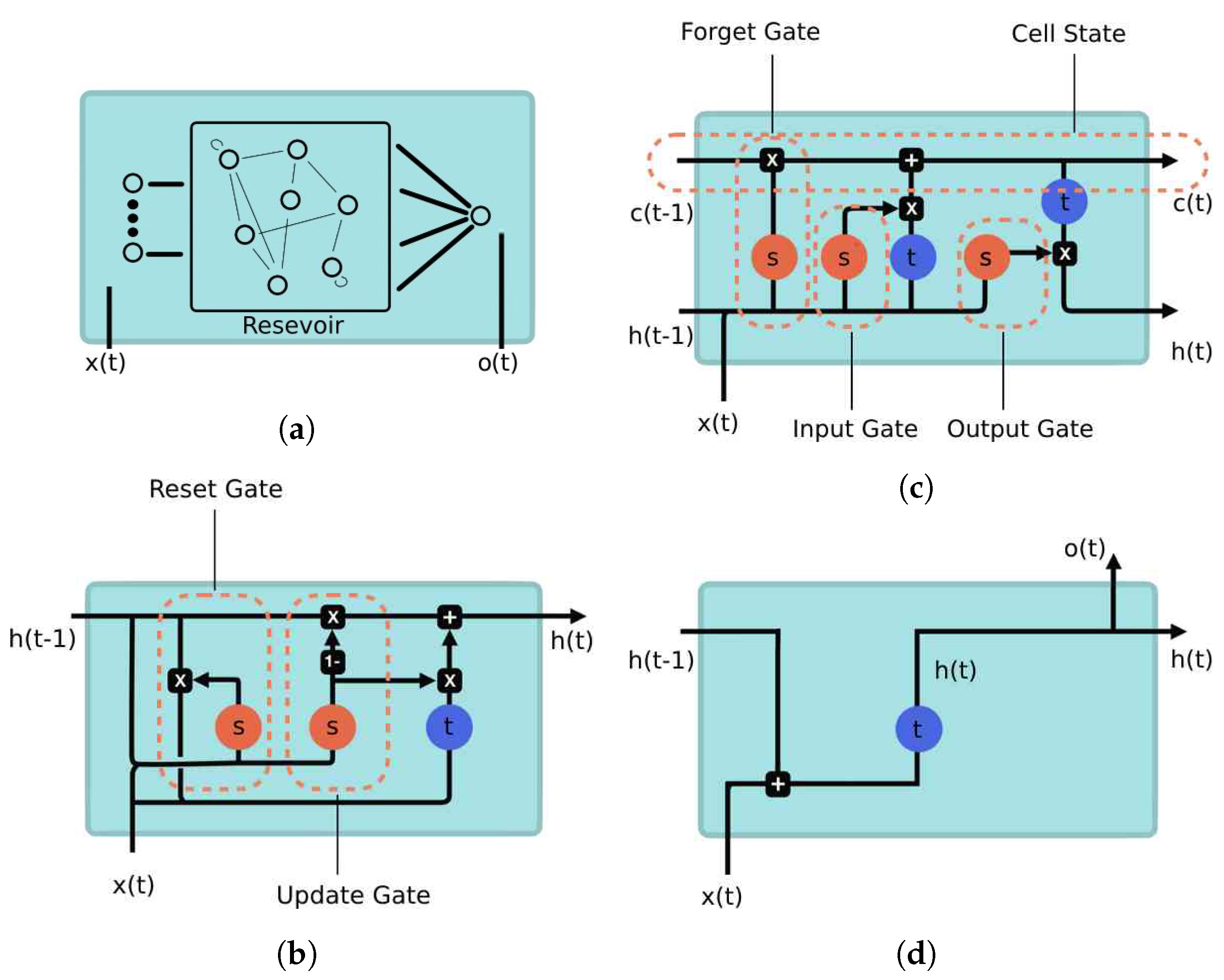
23]. LSTMs incorporate additional processing units, known as memory and forget blocks, which enable the network to selectively retain or discard information over multiple time steps. Gated recurrent unit networks (GRUs) are another variant of recurrent neural networks (RNNs) that offer a simplified structure compared with LSTMs. GRUs aim to address some of the computational complexities of LSTMs while still maintaining the ability to capture long-term dependencies in sequential data.
In a GRU, the simplified structure is achieved by combining the update gate and the reset gate into a single gate, called the “update gate”. This gate controls the flow of information and helps determine how much of the previous hidden state should be updated with the current input [18].
Several studies have been conducted using the aforementioned neural network algorithms in the context of urban and metropolitan areas. In [13], for instance, a standard recurrent neural network model is compared with a multiple linear regression and a feed-forward network to predict concentrations of PM10, showing that the former algorithm provides better performance. As another example, in [11], the authors compare the performances of a multilayer perceptron with those of a long short-term memory network in predicting concentrations of PM10 based on data acquired from five monitoring stations in Lima. Results show that both methods are quite accurate in short-term prediction, especially in average meteorological conditions. For more extreme values, on the other hand, the LSTM model results in better forecasts. More evidence can also be found in [24] and [12], where convolutional models for LSTM are considered, and in [25], where different approaches to defining the best hyperparameters for an LSTM are analyzed. Similarly, in [18], the authors develop architectures based on RNN, LSTM, and GRU, putting together air quality indices from 1498 monitoring stations with meteorological data from the Global Forecasting System to predict concentrations of PM10; results confirm that the examined networks are effective in handling long-term dependencies. Specifically, the GRU model outperforms both the RNN and LSTM networks. On the other hand, LSTM including spatiotemporal correlations in applications with a dense urban network of measurement stations significantly improves forecast performance [23] and may be further exploited to forecast air pollution maps [26].
Another neural methodology used in this study is Echo State Networks (ESNs). The architecture of ESNs follows a recursive structure, where the hidden layer, known as the dynamical reservoir, is composed of a large number of sparsely and recursively connected units. The weights of these units are initialized randomly and remain constant throughout the iterations. The weights for the input and output layers are the ones trained within the learning process. In [27], an ESN predicts values of PM2.5 concentration based on the correlation between average daily concentrations and night-time light images from the National Geophysical Data Center. Hybrid models can also be considered to improve the performance of an ESN model, as in [28], where an integration with particle swarm optimization is performed, and in [29], where the authors manage to further optimize computational speed.
In conclusion, neural networks appear to be a viable approach for obtaining reliable forecasts of pollutant concentrations. However, the performance of the network often depends on architectural features, as well as the quality of the acquired data. One of the shortcomings in existing works that we have addressed is the reliance on traditional time series forecasting methods that consider only historical measurements up to a specific time point [12,30] or deterministic model forecasts [9,
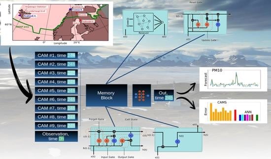
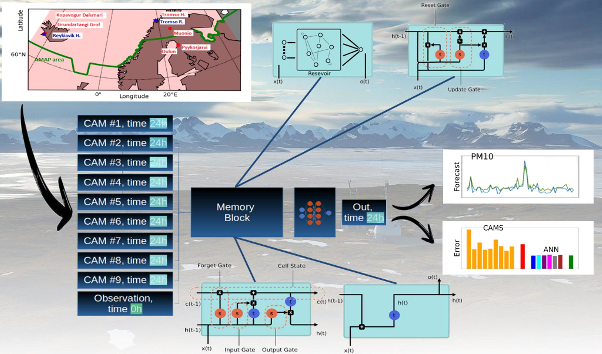
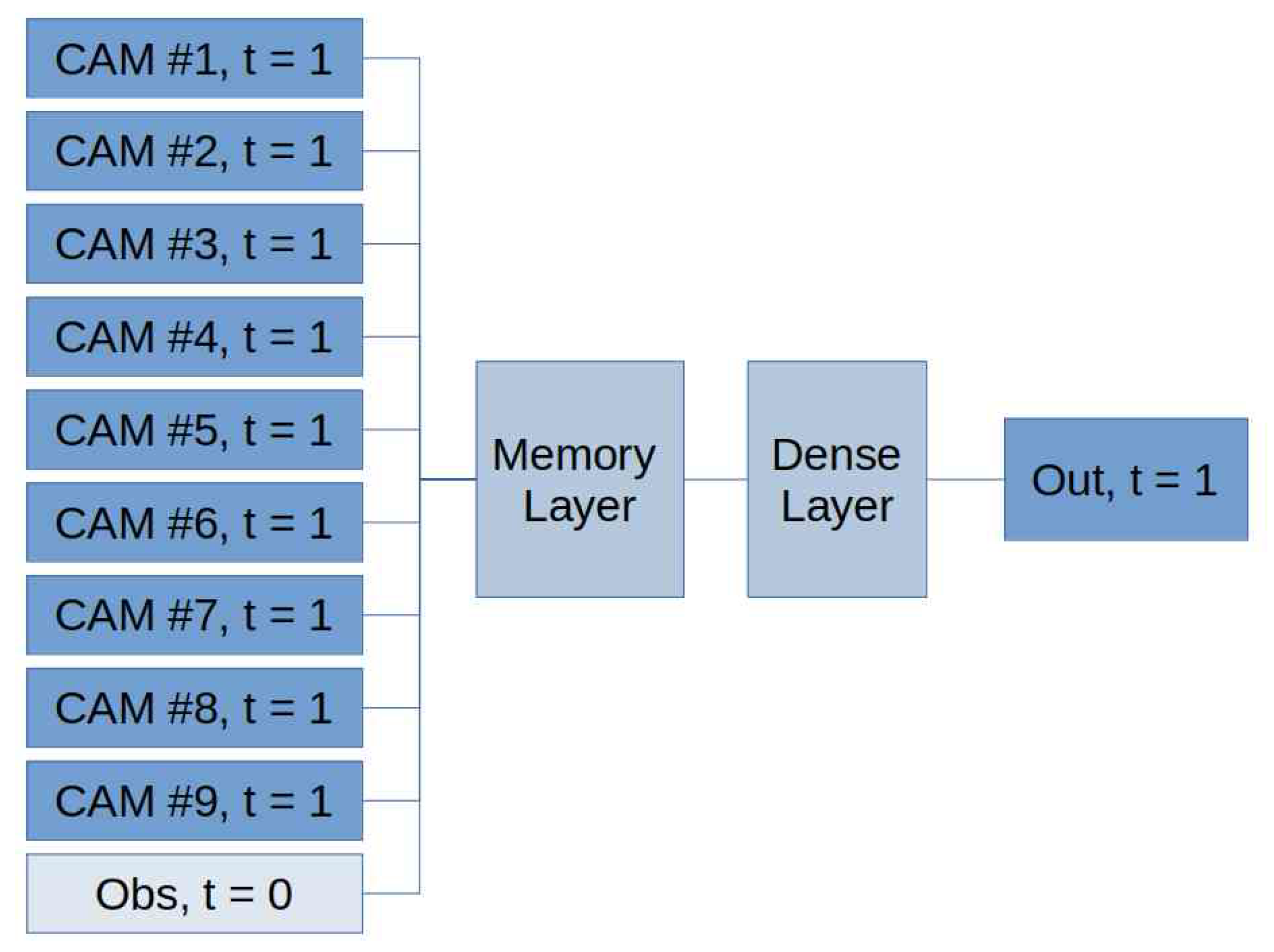
31]. In contrast, our new architecture leverages the availability of observational and model data at different times, allowing for a more comprehensive and dynamic analysis of the underlying patterns and trends, as shown in Section 2.3. In our comparative study, we show that the proposed approach allows us to more accurately capture the temporal dynamics of the data and improve the performance of our forecasts.

Paper Plan

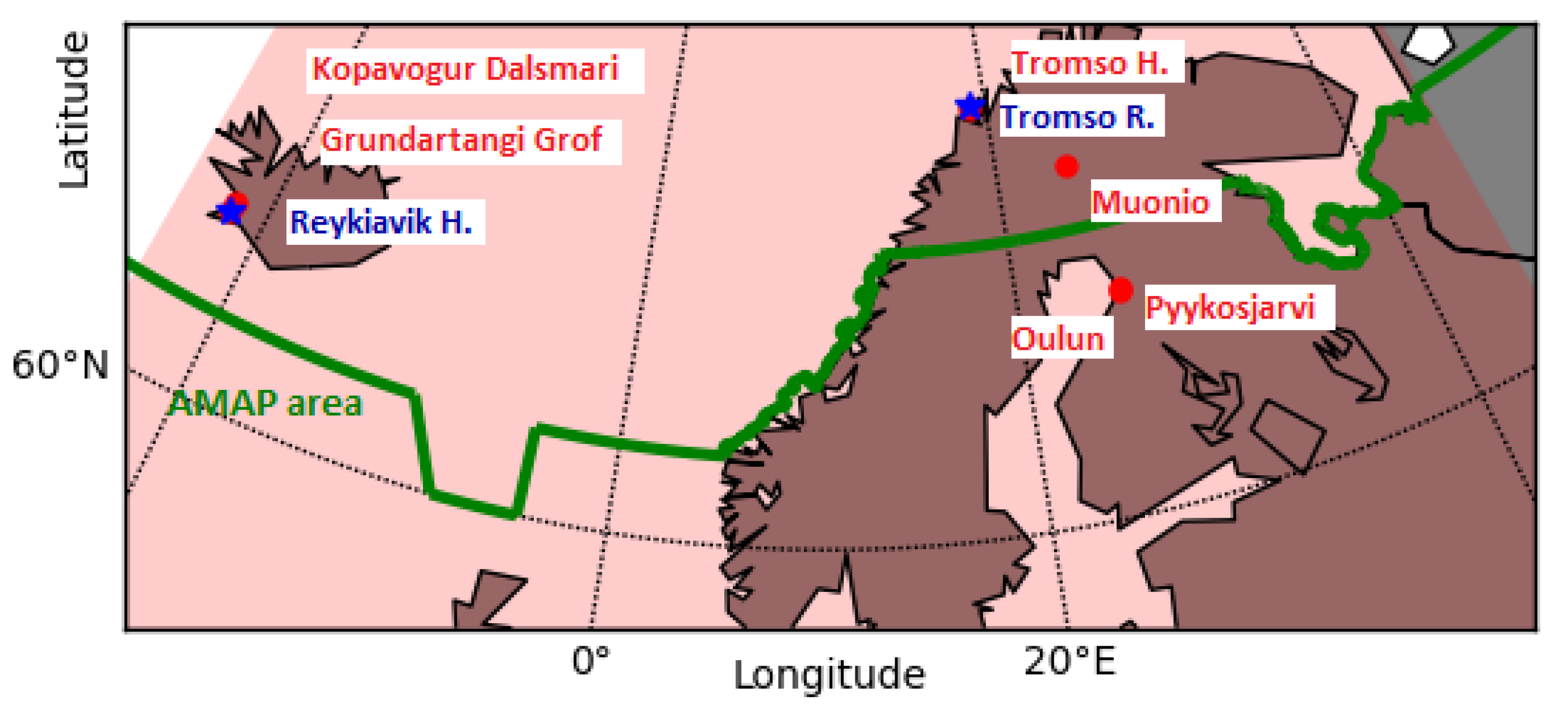
In the upcoming sections, we evaluate the performance of six distinct memory cells. Our study utilizes two components as input time series: (i) measurements of PM10 concentration recorded at 00:00 UTC from six stations situated in the Arctic polar region within the AMAP area and (ii) PM10 forecasts generated by CAMS models at 00:00 UTC for the next day.
In Section 2, we provide an overview of data acquisition and processing, describe the structure underlying the architecture, including details of each ANN design, and outline the technical aspects of implementation.
In Section 3, we present the results and compare the performance of the aforementioned architectures.
In Section 4, we present our discussion and draw our conclusions.

2. Materials and Methods

2.1. Station Data

In the framework of this study, we selected six air quality monitoring stations of the European Environmental Agency (https://discomap.eea.europa.eu/map/fme/AirQualityExport.htm, EEA, accessed on 24 June 2023) and Finnish Meteorological Institute (https://en.ilmatieteenlaitos.fi/download-observations, FMI, accessed on 24 June 2023), collecting hourly measurements of PM10 concentrations ( μ g/m 3 ). The chosen stations are located inside and close to the Arctic Monitoring and Assessment Program (AMAP) area, which defines the physical, geographical, and political boundaries of the Arctic [32]. The AMAP area includes terrestrial and marine regions north of the Arctic Circle (66°32’N), modified to cover the marine areas north of the Aleutian chain, Hudson Bay, and  parts of the North Atlantic Ocean, including the Labrador Sea.
We selected the Arctic monitoring stations which measured PM10 concentrations at hourly frequency during the January 2020–December 2022 period and produced time series with only scarce and short temporal gaps (Table 1, Figure 1). The completeness of the PM10 time series represents a fundamental condition for our prediction experiments, since missing data could degrade the performance of the ANN [33]. Other stations are located in the AMAP area, but the measured PM10 concentration records were not sufficiently long and complete for the application of the ANN. From the time series produced by the chosen monitoring stations, we extracted the concentrations measured at 00:00 UTC for each day. This choice allowed to provide the ANN with PM10 measurements performed at the same time as the CAMS models forecast at 00:00 UTC basetime. The six selected stations are situated in areas with different environmental conditions and emission sources; for this reason, they can be considered representatives of different Arctic contexts. Stations in Grundartangi Gröf, Kópavogur Dalsmári (Iceland), Oulu (Finland), and Tromso (Norway) are located in urban areas and close to the Atlantic Ocean coast, while the station in Muonio (Finland) is positioned in a remote area far from the ocean, representative of background pollution levels. Two stations in Oulu (Finland) located south of the border of the AMAP area are chosen to additionally validate the methodology. The Oulu stations are located a few kilometers away, and their measurements may be spatially and temporally correlated, while other stations are distant from each other. Nevertheless, we assume that time series at each station are independent and do not incorporate spatial correlations in the ANN design.

2.2. Model Data

CAMS provides forecasts of the main atmospheric pollutant concentrations over Europe, available at hourly frequency starting at 00:00 UTC on a daily basis [34]. They are produced once a day by eleven state-of-the-art numerical air quality models employed at different research institutions and weather services in Europe. In the framework of this study, we use the CAMS model forecast at 24 h.
Forecasts produced by different models are interpolated on the regular latitude–longitude grid with a horizontal resolution of 0.1° × 0.1° and are available from the Copernicus European Air Quality service (https://www.regional.atmosphere.copernicus.eu/, accessed on 24 June 2023).
Only nine Copernicus models provide air quality forecasts between January 2020 and December 2022 with only short temporal gaps. Models differ from each other by applying distinct theoretical solutions for estimating the spreading of pollutants and chemical reactions in the atmosphere and have several horizontal and vertical resolutions. Analyses by all models combine information from model forecasts and measurements, but they use different observational datasets and techniques for data assimilation [35]. Table 2 lists the major characteristics of the models used. Surface emissions of pollutants are estimated differently by each model, and all of them use long-term estimates of anthropogenic emissions that do not account for actual daily emission variability [35].

2.3. Definition of Input State for the ANN

Here, we apply a novel approach that consists in providing the ANN with the input state, including both the in situ observation and nine 24 h CAMS model forecasts. The input state consists of a temporal sequence of vectors representing daily forecasts of PM10 concentrations. Each of these vectors contains ten elements with nine 24 h forecasts by each CAMS model (referred as time t = 1 in Figure 2) and the present observation (referred as time t = 0 in Figure 2). This choice differs from previous studies in which the input states of machine learning algorithms used to predict PM10 levels were derived either only from previous observations at monitoring stations [12,30] or only from models forecasts [9,31]. Here, we show that the combination of the last available observation and the ensemble of CAMS model forecasts improves the ANN forecast performance. For instance, in cases where the CAMS models fail to detect a sudden change in emissions near the monitoring site, incorporating the latest observation can assist the ANN model in adapting its forecast (see Section 3.1).

2.4. Data Preprocessing

To address the technical difficulties resulting in the data gaps mentioned earlier, preprocessing of the input data is necessary to ensure temporal continuity. If the data gaps span multiple time points, the dataset is adjusted by cropping it to avoid such large gaps. In cases where only a single time point is missing, the missing data are interpolated using linear interpolation based on the previous and subsequent data points. Furthermore, prior to being fed into the classification pipeline, the input data are normalized, and after processing, they are denormalized. This normalization step helps ensure consistent scaling across the features. To confirm the stationarity of all measurement series, an augmented Dickey–Fuller test is conducted. This test is performed to assess the presence of trends or unit roots that may affect the analysis and modeling process (Stationarity is an essential assumption for forecasting algorithms such as SARIMAX. However, it also can be beneficial with other forecasting methods, including machine learning approaches [36,37]).

2.5. General Architecture

In this study, we propose a design that comprises an input layer, a memory layer, a dense layer, and an output layer (see Figure 2). The input consists of nine sets of values provided by the CAMS, and with one set of measurements. To enhance the accuracy of the predictions, we incorporate 24 h CAMS (referred as time t = 1 in Figure 2). As stated in the earlier sections, this architectural decision yields improved results in terms of mean squared error (MSE) (In Appendix C, we provide a specific case that demonstrates that using mean absolute error (MAE) instead of mean squared error (MSE) does not impact the cross-comparison evaluations).
Figure 2. General architecture. ’CAMS #n’ indicates the nth CAM model.
Remotesensing 15 03348 g002
The memory cell in our architecture is implemented using various specifications, i.e., echo state networks (ESNs), long short-term memory networks (LSTMs), gated recurrent units (GRUs), standard recurrent neural networks (RNNs), and windowed multiperceptron (with time window sizes of 4 and 1 time steps). We briefly provide some details on these different specifications below. In addition to the approach described in Figure 2, we also explored alternative designs: SARIMAX, multiple memory layers and multiple memory cells per layer, feeding our algorithm with multiple time steps in input and output while training. All these attempts did not yield any performance benefits in terms of MSE or provide additional insights. In particular, for SARIMAX, we report results in Appendix B comparing the MSE and graph with the LSTM case. In the following, we provide a concise summary of our design. For a more comprehensive description, including the relevant mathematical details, please refer to Appendix D.

2.5.1. Memory Layer

The memory layer plays a crucial role in storing the temporal information present in the input sequence. In our study, we explored six popular solutions.

Echo State Networks

The ESN approach (Figure 3a) [38] sets the weights of the recurrent layer, called “reservoir”, in such a way that the recurrent hidden units effectively capture the history of past inputs, while only the weights of the output layer are trained. The key question in this case is how to choose the weights of the recurrent layer. First, connections among the recurring units should be sparse, resulting in a sparse square weight matrix. Additionally, the spectral radius of the matrix should be kept low, ideally less than 1 (as in our implementation), to contribute to the echo state property, as described in [39] (in [40], it is stated that a spectral radius of less than 1 is neither sufficient nor necessary for the echo state property). However, in combination with carefully chosen activation functions such as tanh(), it can be allowed to exceed 1. This mechanism enables the propagation of information through time. Proper tuning of hyperparameters is essential for generating echoes that accurately reflect the input content, and tools provided in [39,41] can aid in this process. We train our ESN using gradient descent similarly to the algorithms presented in [42].

Long Short-Term Memory

Standard RNN cells (see Section “Recurrent Neural Networks”) suffer from well-known limitations, including vanishing and exploding gradients during training with backpropagation. To address these issues, long short-term memory (LSTM) cells were developed, offering a more sophisticated approach to managing the hidden state. Figure 3c illustrates its structure. The rectangular boxes represent activation functions applied prior to matrix multiplications (not depicted in the figure). The circular spots indicate element-wise operations. The variables x t , h t , and  c t denote the input, hidden state, and cell activation vector, respectively. The function σ represents the sigmoid activation function. The cell output is computed by applying a sigmoid activation function to a weighted sum of x t , h t 1 , and a bias term. Figure 3c also highlights the internal architecture of LSTM, which incorporates Input, Forget, and Output Gates. Confluences in the figure represent concatenations, while bifurcations denote element-wise copying. Taking into account these details and referring to the illustrated diagram (Figure 3c), it is possible to derive the corresponding equations.

Gated Recurrent Units

GRU cells are a simplified version of LSTM, offering comparable performance for modeling tasks. They are particularly advantageous with small datasets, since they have a smaller parameter count. Figure 3b depicts the overall structure of a GRU cell, emphasizing the presence of the Reset and Update Gates.

Recurrent Neural Networks

The standard RNN is based on the original recurrent approach (see Figure 3d). It operates by combining an input x(t) with the previous hidden state h(t−1), which is then passed through an element-wise tanh() cell (depicted as the rounded block labeled with t). The resulting output is stored as the next hidden state h(t) and also serves as the output o(t). In the figure, bifurcations represent component-wise copies before being multiplied by weight matrices and added with biases. Operations such as addition (+) are applied prior to multiplying with weight matrices and adding biases. This recurrent scheme was historically the first proposal capable of storing variable-length information from a time series.

Multilayer Perceptron

In this study, a multilayer perceptron (MLP) with a configuration of 5 units in the hidden layer and 1 unit in the output layer is employed. Two different implementations of the MLP are considered: one utilizes four time steps from the input data sequence, while the other utilizes only one time step.

2.5.2. Implementation Details

Our implementation utilizes Keras for the RNN, LSTM, GRU, WMP, and WMP4 models and TensorFlow for the ESN model. To ensure a fair comparison among these six methods, we carefully selected the hyperparameters, which are outlined in Table 3, Table 4 and Table 5. These hyperparameters were determined solely based on the stations listed in Table 6; each dataset was divided into training and test sets to allow for the selection of optimal values through an iterative procedure. Finally, these stations were subsequently excluded from the validation process to prevent data peeking and potential overfitting.
Validation was performed on the stations listed in Table 1 utilizing the determined hyperparameters. The dataset for these stations covers the time interval from January 2020 to December 2022. However, due to missing observations resulting in significant data gaps, we cropped the datasets according to Table 7. For model validation, we used the last 365 steps, reserving the remaining data for training.
For all cases, we employed the minimum absolute error as the loss function and Adam as the optimizer.

3. Results

In this section, we present the results obtained using measurements and CAMS forecast data from January 2020 to December 2022. The data are divided into training (730 steps) and test (365 steps). In the case of potential single data gaps, linear interpolation was utilized to fill in the missing values. However, if the missing data resulted in larger gaps, the training dataset was cropped to exclude these gaps. The initial time step for each station is provided in Table 7.

3.1. Impact of Temporal Data

In this subsection, we investigate the impact of different choices regarding CAMS and observations on the forecasting performance. We compare the following alternatives:
  • CAMS forecast at 24 h; observation at 0 h (our choice);
  • CAMS forecast at 24 h; no observation;
  • CAMS forecast at 0 h; observation at 0 h;
  • No CAMS; observation at 0 h.
Figure 4 illustrates the results, demonstrating that incorporating in situ observations and CAMS forecast at 24 h yields the best performance in terms of MSE. It should be noted that the presented results are specifically for station Pyykösjärvi (Oulu) (15557), but similar experiments were conducted for all stations, with consistent findings.

3.2. Original Data

In the following subsections, we present our results. Measurements and CAMS forecasts are used as input of our architecture without any additional preprocessing steps applied.

3.2.1. MSE Results

The convexity of the MSE function and the application of Jensen’s inequality guarantee that the MSE of the average of the models is always lower than or equal to the average MSE of the individual models. Hence, in addition to presenting the results of each model, we also provide the MSE of their average. This average can be viewed as an ensemble forecast and can be utilized in practical applications. Our MSE results are reported in Figure 5.
Figure 5 demonstrates that there is no large difference among the memory cells. All the implemented solutions show that the model MSE is less or equal the best available CAMS forecast. Notably, in three instances (e.g., Figure 5b,c,f), the model produces significantly more accurate results compared with the CAMS forecasts.

3.2.2. Forecast Results

In Figure 6, we present the forecasting results. To ensure clarity, we depict the graph of the memory cell that achieved the best performance in terms of MSE, along with the corresponding measurement data. The time interval considered in the plot spans the entire year of 2022.
To further evaluate the performance of the algorithms, we provide a closer examination of the forecasting results for the time interval from the 200th to the 260th day of the year 2022. Figure 7 displays the results obtained from all the memory cells. The shaded area in Figure 7 represents the standard deviation of the forecasted values from the different memory cells relative to their average, indicating variations in the predictions among the different models.
Finally, in Figure 8, we present a comparison between the CAMS forecast, our model, and the measurement data for the station with code 15609. The last row of the graph represents our model’s forecast, while the rows above display the CAMS forecasts.

3.3. Filtering the Input Data

While Figure 5 illustrates that our model either matches (Figure 5a,d,e) or clearly outperforms (Figure 5b,c,f) the best CAMS, Figure 7 reveals variations in the performance of our architecture depending on the specific station under consideration. Notably, there is a stark contrast in forecast quality between Figure 7b,d, with the latter displaying significant differences (shaded area) among the utilized memory cells (also apparent in Figure 5d).
In the literature [43,44,45,46], it is common practice to utilize a log-normal distribution for interpolating PM10 data histograms. In our study, we adopt this assumption to handle outliers in our dataset by replacing them with the temporally nearest data points. The algorithm used for this purpose is provided in Appendix A.1. In Figure 9, the data points to be removed are indicated by the region on the right-hand side of the vertical dashed line (colored dark/red). Appendix A.2 displays the histograms and the cutting thresholds of all the stations listed in Table 1.

3.4. Filtered Data

In the following subsections, we present our results using outlier-filtered input data, evaluating both the mean squared error (MSE) and the forecasting performance.

3.4.1. MSE Results

In the following, we report our results in terms of MSE (Figure 10) and forecasting (Figure 6).

3.4.2. Forecast Results

Figure 11 illustrates the forecast details for the time interval from the 200th to the 260th day. Specifically, Figure 12 focuses on the case of station 52109. In the scenario without data filtering, the echo state network (ESN) model exhibits the highest mean squared error (MSE), while the long short-term memory (LSTM) model performs the best. However, when the data are filtered, both the ESN and LSTM models show improved performance and have similar MSE values. Removing outliers from the data significantly enhances the forecast quality of both memory cell models. Notably, the mentioned significant difference in terms of MSE between the ESN and LSTM models (as observed in Figure 5d) corresponds to the noticeable difference in their forecasting, as depicted in Figure 12a. The ESN memory cell appears to be more affected by outliers compared with the LSTM.
On the other hand, filtering measurements with high pollution concentration further improves the prediction performance of the artificial neural network (ANN) in terms of MSE compared with the CAMS model forecasts and the persistence model (Figure 10). When using the filtered dataset, the persistence model demonstrates better prediction performance than any of the CAMS model forecasts (Figure 10), while with unfiltered measurements, the CAMS model forecasts outperform the persistence model (Figure 5). This indicates that, in comparison with persistence, the CAMS forecasts also improve when spikes are removed. However, regardless of whether the measurements are filtered or not, the predictions of the artificial neural network (ANN) consistently show significantly higher accuracy.
The fact that different memory cells show similar performances aligns with the existing literature on PM10 forecasting in non-Arctic regions, which model PM10 forecasting tasks on Markov chains [47,48]. However, Figure 12 demonstrates that LSTM and ESN react differently to outliers. Although we did not make hypotheses about the origin of these outliers, these results suggest that outliers introduce higher-order non-Markovian contents that pose challenges for the ESN cell but can be effectively utilized by the LSTM cell.

4. Discussion and Conclusions

In this study, we conduct an in-depth analysis of a 24 h forecasting design for PM10 concentrations that leverages both in situ measurements and forecasts generated by deterministic models. This utilization of input data consisting of measurements and model forecasts at different times introduces a novel perspective to the task at hand, enhancing the predictive capabilities of the algorithms employed. Furthermore, it offers a valuable contribution to the existing literature by demonstrating the potential of incorporating multitemporal data in time series forecasting.
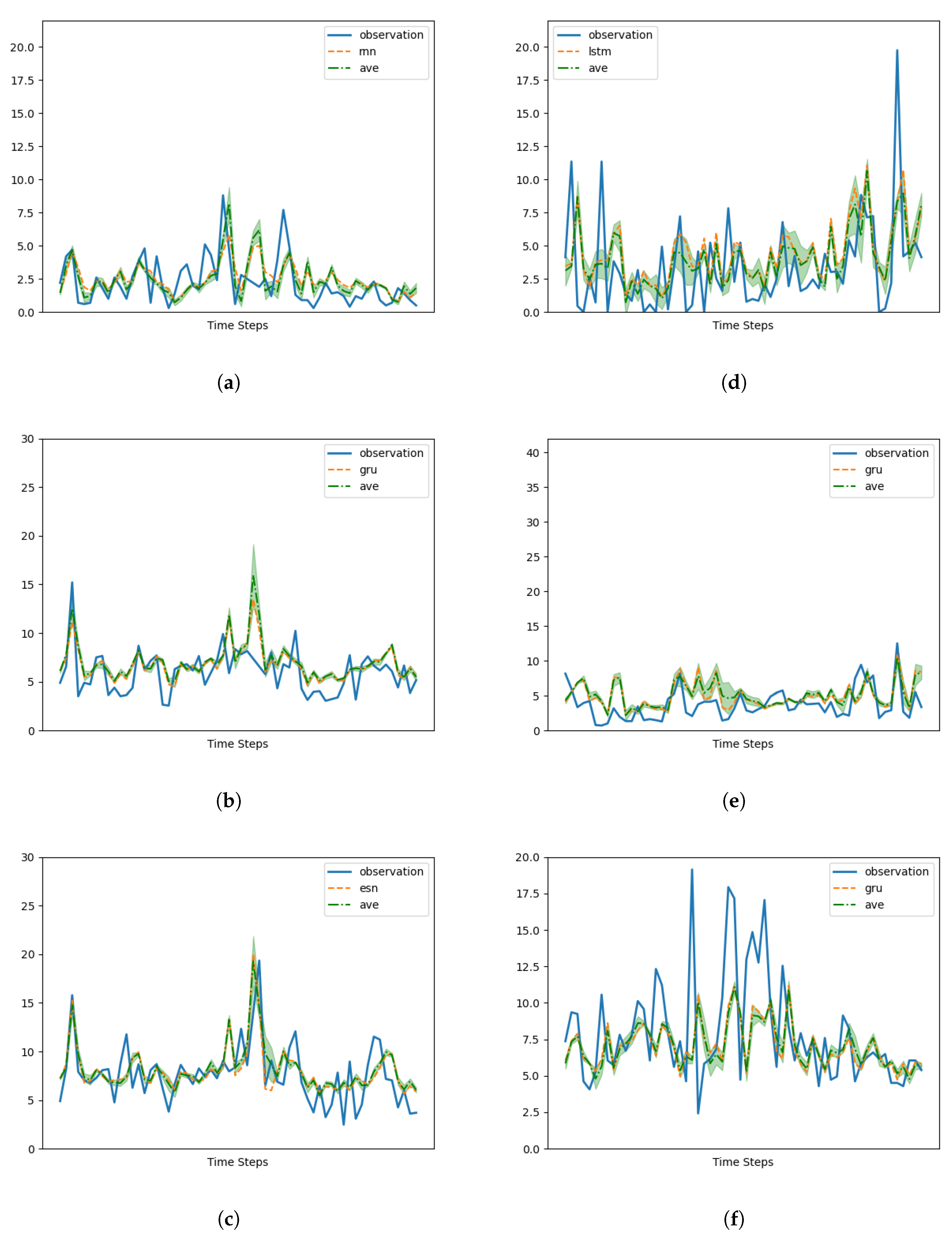
Central to the design are the memory cells, which serve as alternative options for modeling the data and improving forecasting accuracy. Specifically, we explore the utilization of echo state networks (ESNs), long short-term memory (LSTM), GRUs (gated recurrent units), and recurrent neural networks (RNNs), as well as four-step and one-step temporally windowed multilayer perceptron.
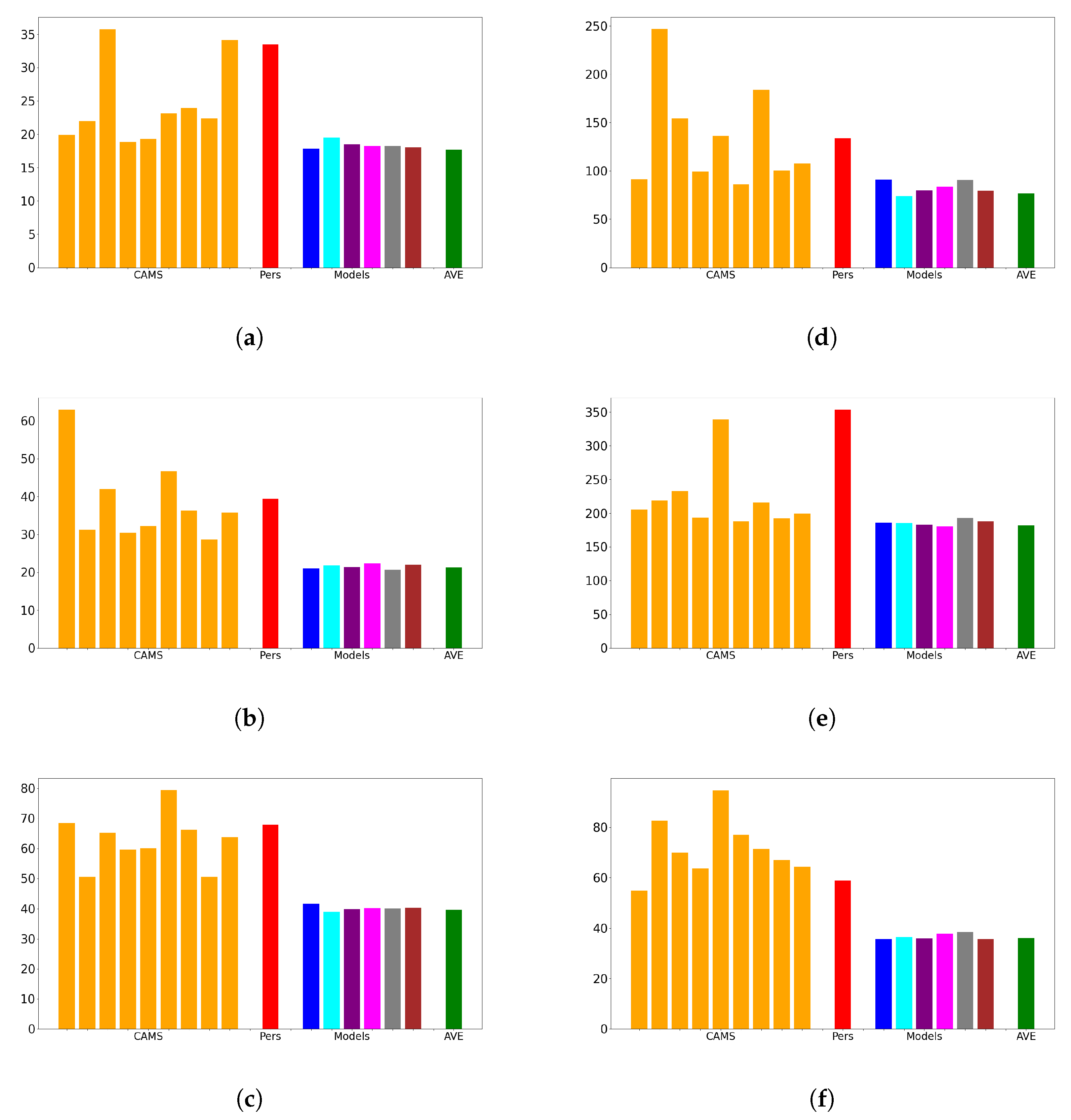
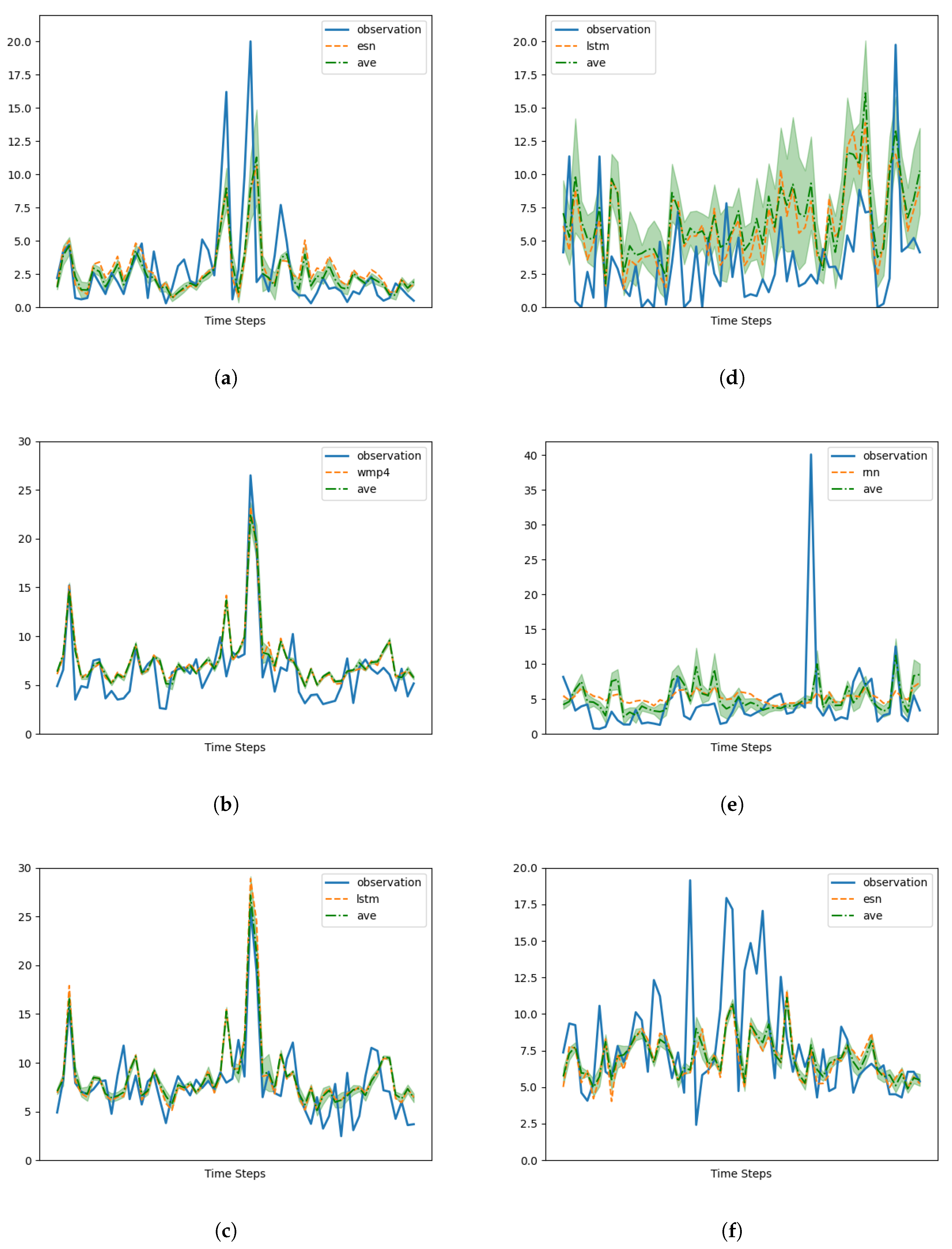
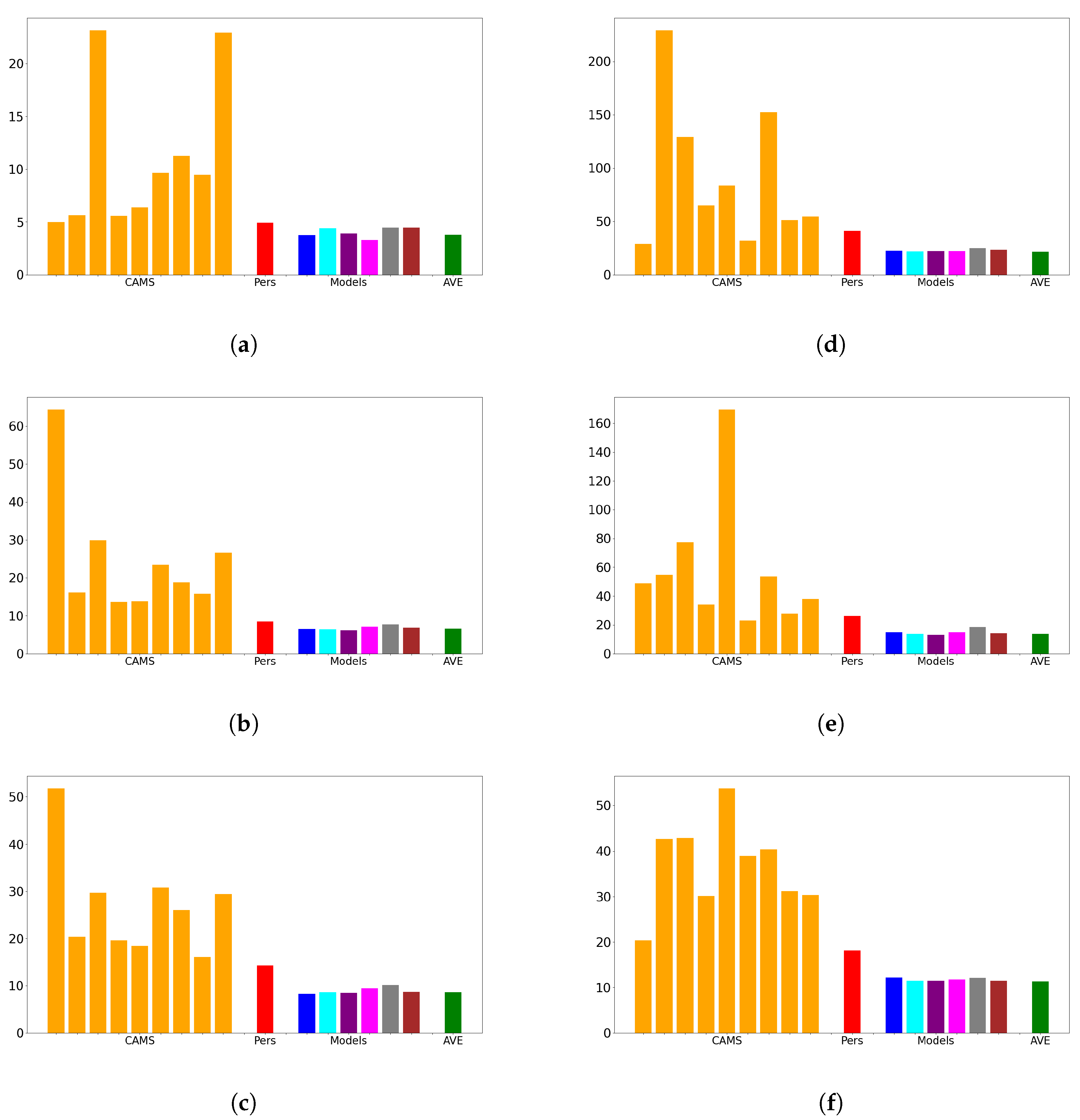
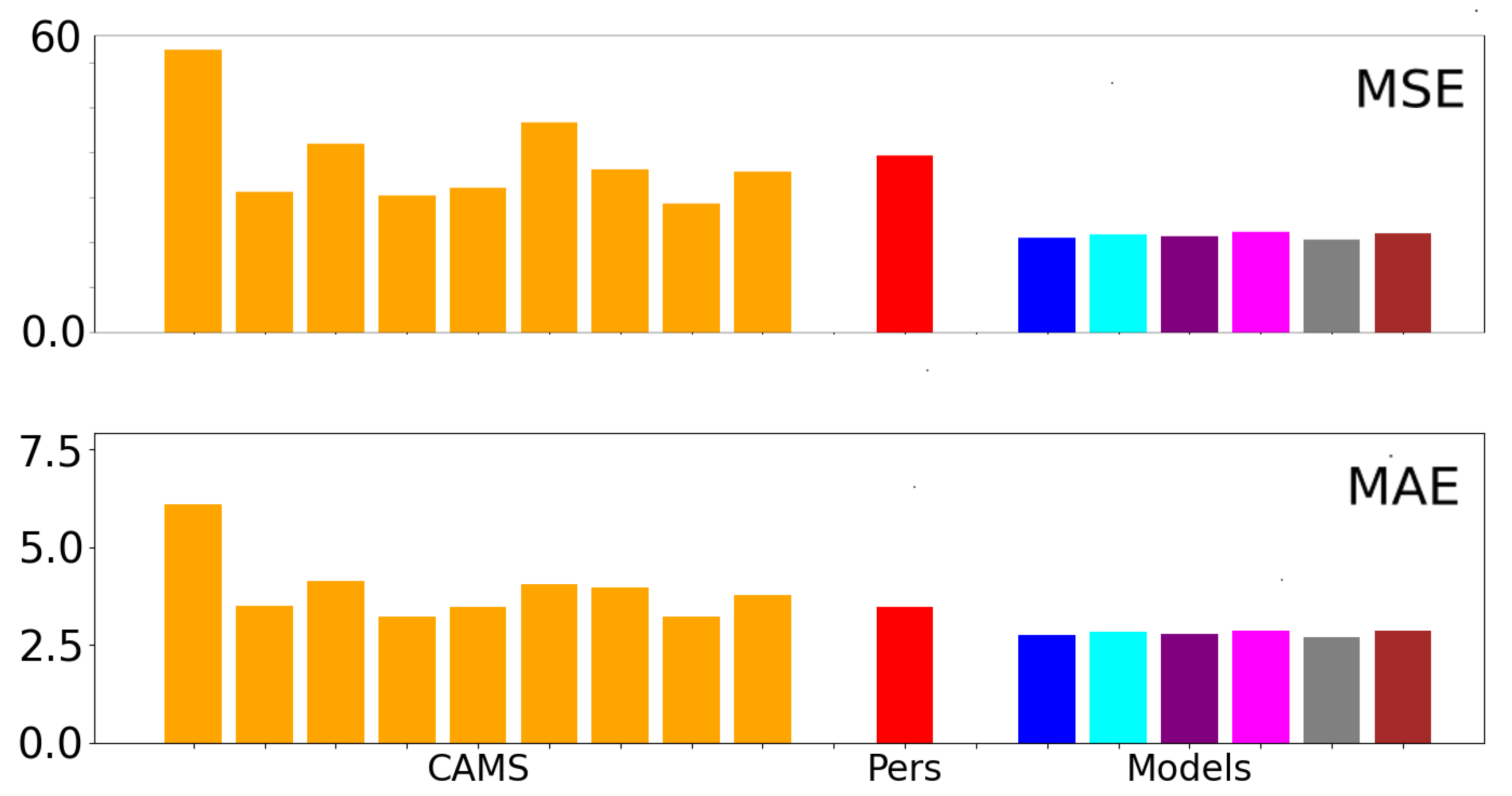
Our architecture exhibits remarkable performance by effectively capturing the strengths of either the CAMS or measurements, regardless of the specific memory cell employed. It consistently outperforms the CAMS, resulting in significant average improvements ranging from 25% to 40% in terms of mean squared error (MSE). This demonstrates the effectiveness of the design in harnessing the predictive capabilities of the alternative memory cells.
However, it is important to note that the choice of the memory cell has a substantial impact on the forecasting capability of the design when dealing with data series characterized by intricate behavior.
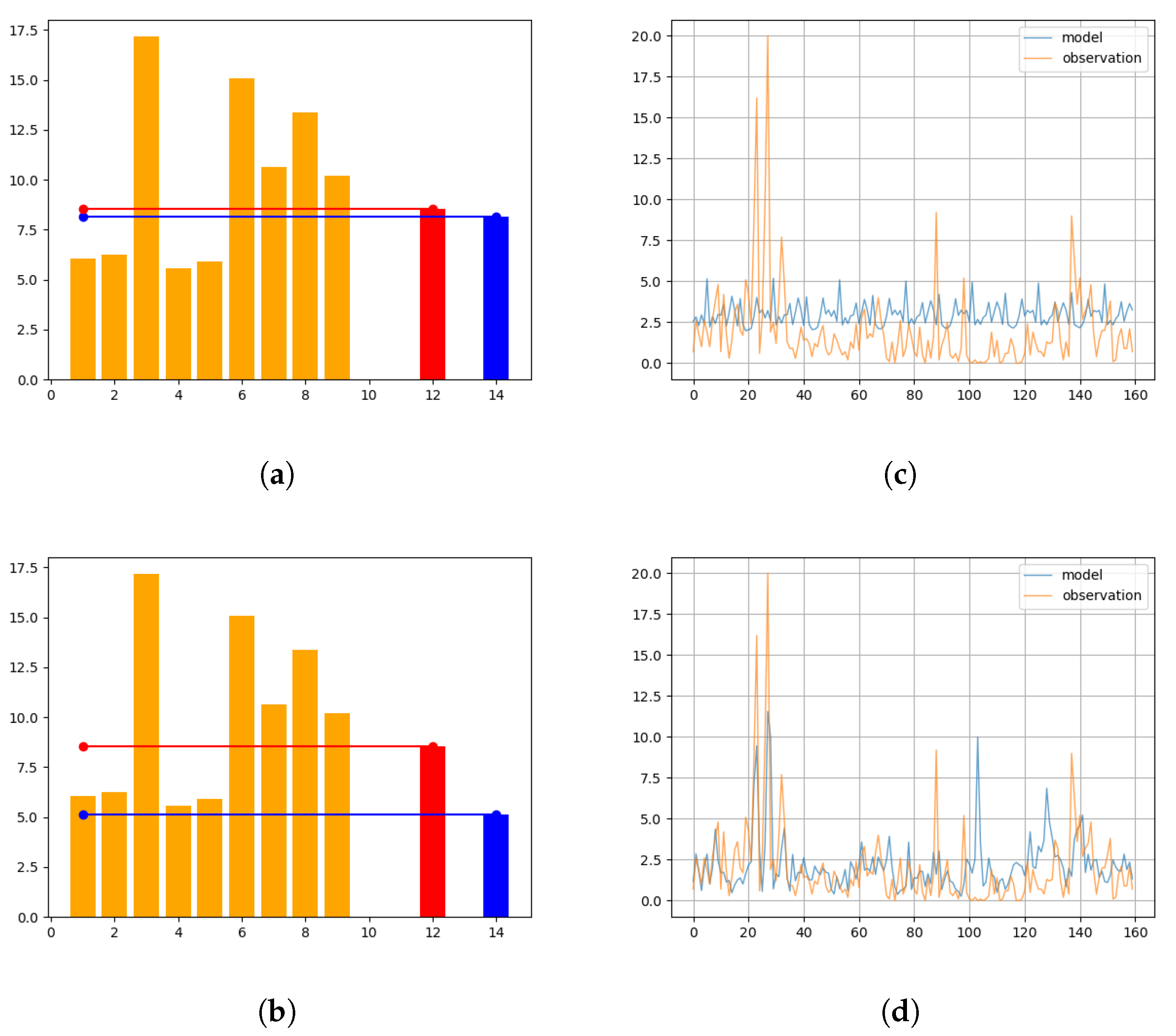
Furthermore, we investigated the impact of outliers as a potential source of error and assessed how their removal significantly affects the forecasting capability of our model.
While our proposed approach has shown effectiveness in our tests, there are limitations that should be acknowledged. These include the simplistic method of combining memory cell contributions (simple average) and the limited input data considering only PM10 observations without accounting for the relationship between pollutant concentrations and chemical constituents.
Therefore, future research endeavors can explore the integration and fusion of the distinct strengths exhibited by different memory cells, going beyond the conventional approach of simply averaging their results. By developing an ensemble design that selectively leverages the best options based on the specific characteristics of the data series to be forecast, we can further enhance the overall forecasting performance and reliability of the system. Additionally, an interesting avenue for exploration in future studies could involve redesigning the ANN model to incorporate spatiotemporal correlations among nearby monitoring stations (for instance inserting graph neural networks [49] or graph networks [50] at the beginning of the forecasting pipeline) and the PM10 chemistry composition, potentially providing valuable insights into the relationship between pollutant concentrations and chemical constituents. Such investigations have the potential to enhance our understanding of air quality dynamics and improve the accuracy of PM10 forecasts.
Based on our results in Section 3.4.2, we interpret that the PM10 Arctic observations exhibit predominantly Markovian behavior, where the future evolution of the underlying dynamic system depends primarily on the present state. However, 
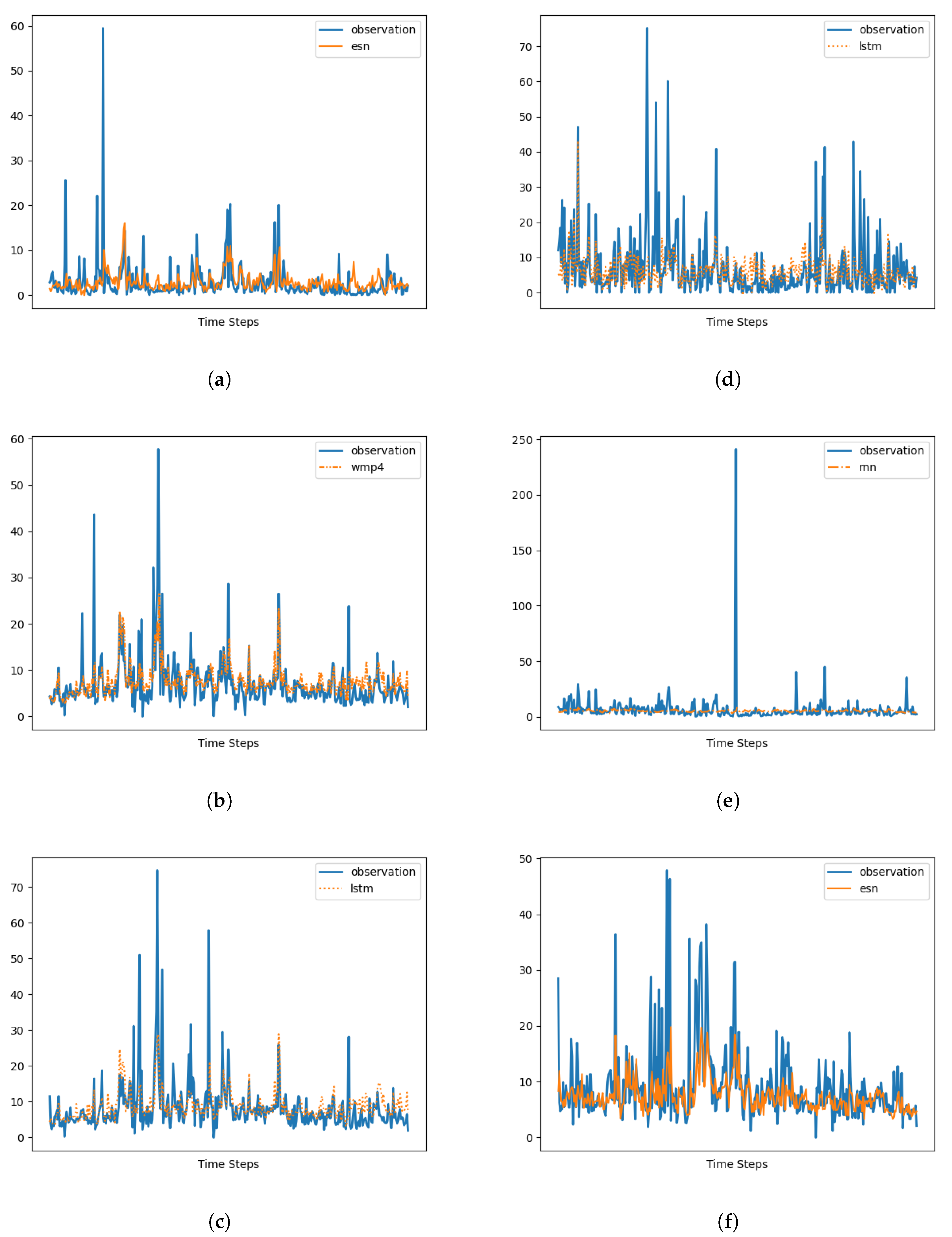
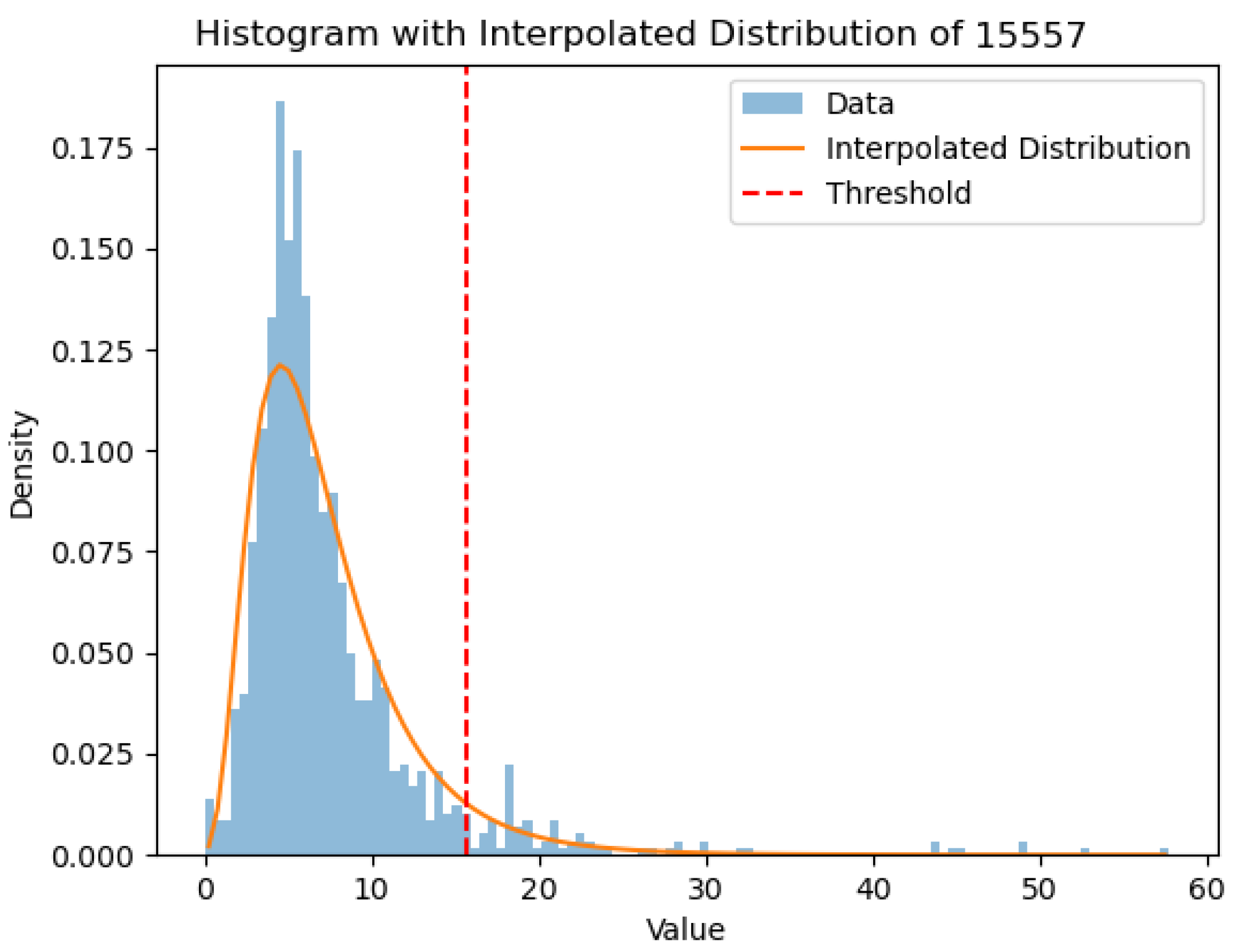
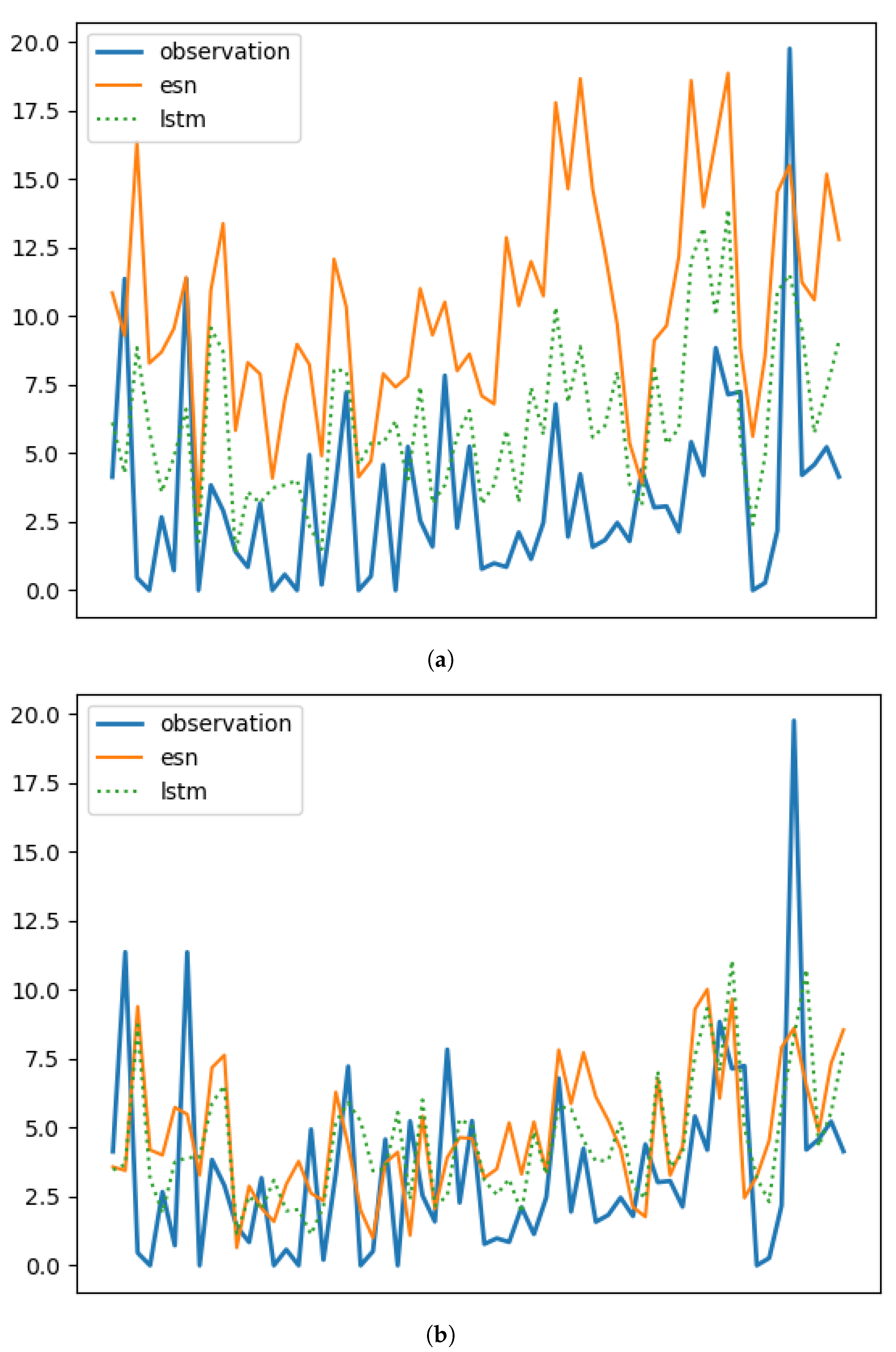
Figure 11 demonstrates that two non-Markovian memory cells, namely LSTM and ESN, react differently to outliers. Specifically, ESN shows poorer performance in the presence of outliers, while LSTM performs best among all the memory cells. 
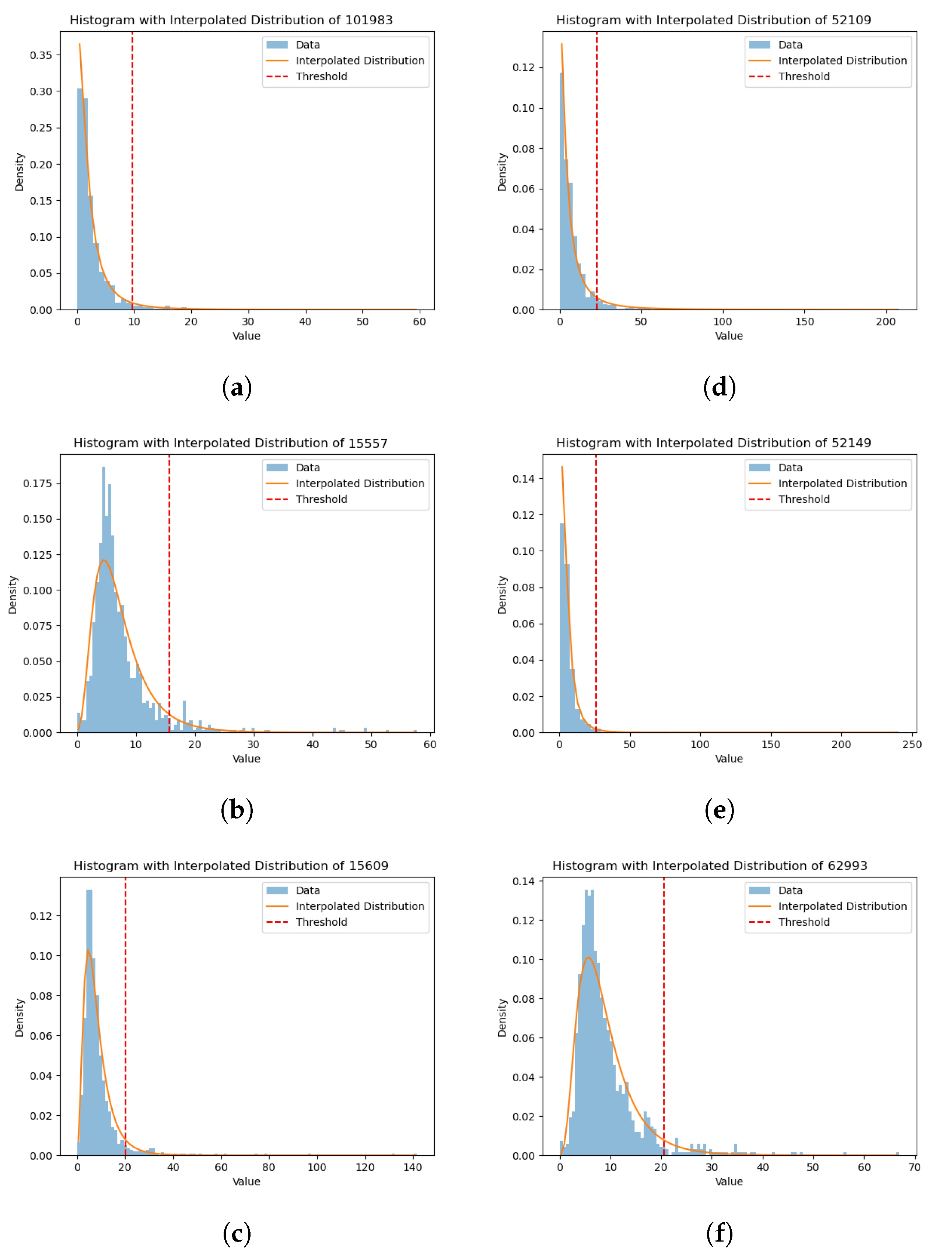
Figure 11 also illustrates that the performances of the two cells are comparable only when the outliers (i.e., values deviating from the log-normal distribution) are filtered out. Although we did not make hypotheses about the cause of these outliers, these results suggest that outliers introduce higher-order non-Markovian contents that pose challenges for the ESN cell but can be effectively utilized by the LSTM cell. Therefore, as another interesting topic for future research, it would be valuable to investigate the presence of outliers in the data, their nature, and their impact on the non-Markovian nature of the underlying dynamics. This research could potentially lead to improved modeling techniques that can effectively handle outliers and prevent large or catastrophic events.

Author Contributions

Conceptualization, S.D., P.F. and A.P.; methodology, P.F.; software, P.F.; validation, S.D., P.F., M.M. and A.P.; formal analysis, S.D., P.F. and M.M.; investigation, P.F.; resources, E.F.C. and F.P.; data curation, S.D., I.C. and P.F.; writing—original draft preparation, I.C., A.C., P.F. and S.D.; writing—review and editing all authors; visualization, P.F.; supervision, M.M.; project administration, P.F.; funding acquisition, E.F.C., A.P. and F.P. All authors have read and agreed to the published version of the manuscript.

Funding

This research was supported by the Arctic PASSION project under the European Union’s Horizon 2020 research and innovation programme grant agreement No. 101003472.

Data Availability Statement

Input in situ observations are available from EEA and FMI, while model forecasts are available from Copernicus (see Section 2). Data produced in the study are available from the authors upon request. The python code of this study is open sourced at https://github.com/pfaz69/ForecastPM (accessed on 24 June 2023).

Conflicts of Interest

The authors declare no conflict of interest. The information and views set out are those of the authors and do not necessarily reflect the official opinion of the European Commission.

Appendix A

Appendix A.1

In the algorithm, the function c a l c u l a t e _ o p t i m a l _ t h r e s h o l d is based on the assumption that the expected data distribution should fit the log-normal. This assumption translates to replacing the outliers in the observation data with the temporally nearest data: the algorithm finds the optimal threshold to correspondingly cut the histogram. The position of this threshold is calculated to minimize the MSE between the histogram of the new data and the corresponding log-normal distribution.

Appendix A.2

Algorithm A1 results are plotted in Figure A1.
Algorithm A1 ComputeOptimalThsh
1:
procedure ComputeOptimalThsh(file_data)
2:
   y , _ read _ data ( f i l e _ d a t a )
3:
   num _ bins length ( d a t a ) ÷ 10
4:
   hist , bin _ edges create _ histogram ( d a t a , num _ bins )
5:
   p a r a m s fit _ ognormal _ distribution ( d a t a )
6:
   optimal _ threshold _ quantile optimize _ threshold _ quantile ( d a t a , hist , hist , bin _ edges )
7:
   optimal _ threshold calculate _ optimal _ threshold ( d a t a , optimal _ threshold _ quantile )
8:
  return  optimal _ threshold
9:
end procedure
Figure A1. Simulation results (filtered MSE). See Table 1 for code reference: (a) 101983. (b) 15557. (c) 15609. (d) 52109. (e) 52149. (f) 62993.
Remotesensing 15 03348 g0a1

Appendix B

We tested SARIMAX to exploit eventual seasonal patterns, considering the possibility of seasonality in our data, although it was not immediately evident. To identify the most effective SARIMAX hyperparameters, we employed grid search, which involved systematically evaluating various combinations of the hyperparameters’ orders and seasonal orders based on both the Akaike information criterion (AIC) and mean squared error (MSE). We found that the resulting interpolation produced less satisfactory outcomes, generating rather “flat” graphs. Figure A2) reports MSE (left) and forecasting (right) for station code 101983, 160 test steps, for o r d e r = [ 1 , 1 , 1 ] , and s e a s o n a l   o r d e r = [ 2 , 0 , 2 , 12 ] , found using the AIC criterion.
Figure A2. SARIMAX (top row) vs LSTM (bottom row) results in 160 test steps: Left column: the 9 bars on the left show the CAMS MSE; the light color (red) bar shows the persistence MSE; and the last bar on the right shows the model MSE. The right column of the figure shows the algorithms’ time forecast (dark color/blue) vs the observation measurements (light color/orange): (a) SARIMAX MSE. (b) LSTM MSE. (c) SARIMAX forecasting. (d) LSTM Forecasting.
Remotesensing 15 03348 g0a2

Appendix C

Figure A3 shows a comparison of the error histograms when adopting different indicators: MSE and MAE. The two diagrams are reduced to the same size to highlight similarities, but their different scales are shown on the y axis.
Figure A3. MSE vs. MAE.
Remotesensing 15 03348 g0a3

Appendix D

This section gives an overview of the theoretical blueprint of the algorithms developed in our work. As mentioned in Section 2, our analysis involves the comparison of several predictive models which rely on artificial neural network structures, namely:
  • Multilayer perceptron;
  • Recurrent neural network;
  • Gated recurrent unit;
  • Long short-term memory network;
  • Echo state network.
Each one relies on specific architectural features. We now describe the structure of the networks used in our models.

Appendix D.1. Data Processing

The input vector for each of the networks (exception made for the multilayered perceptron with four time steps) consists of observation data at day d, i.e., o b s ( d ) = o b s d paired with CAMS models analyses at times d + 1 . At each time step, the input vector is then given by
x ( d ) = [ o b s d , C A M d + 1 1 , , C A M d + 1 9 ]
The input vector is then normalized by minmax scaling, i.e., fitting the data in the range [0, 1] via the transformation:
x x min { x } max { x } min { x }
In the next few sections, we use the compact notation x to identify the input vector with time dependency as described above.

Appendix D.2. Model Architecture

An artificial neural network consists of several units subdivided into an input layer (given by a data vector), one or more hidden layers, and an output layer, each connected through activation functions.
The number of units per layer, as well as the number of layers, are determined in the hyperparameters tuning phase, as described in Section 2.5.2, and for each architecture, such variables are recapped in Table 3, Table 4 and Table 5. Designs of the different models are represented in Figure 2. All models have weights optimized via gradient descent algorithms, and the loss considered is the mean absolute error.

Appendix D.2.1. Multilayer Perceptron

The model used in our approach consists of three layers: input, output, and one hidden layer. While the model has two types of implementation for a prediction within a time series framework (an input vector with one time step and another one with four time steps), the hidden and output layer structures are identical. The network follows a feed-forward backpropagation model applied to three dense layers.
Let x = { x i } denote the input vector and y the output observation. Let ω k = { ω i k } denote the vector of weights at layer k. The activation functions for the hidden and output layer are denoted by σ 1 and σ 2 , respectively. Considering the input vector as described above and the hidden layer consisting of five units, the output of the network is then defined as
y ^ = g ( x ) = σ 2 j = 1 5 ω j 2 · σ 1 i = 1 10 ω j , i 1 · x i + b j 1 + b 2
where b k are the biases at layer k.
Using backpropagation, the weights at each layer are then updated by means of the error signals, defined from the derivatives of the cost function.

Appendix D.2.2. Recurrent Neural Network

Recurrent neural networks are an upgraded version of forward-propagation networks, where edges within hidden layers may admit connections with units at adjacent time steps. At iteration time t, the vector x ( t ) = x t denotes the input vector (i.e., the time step t within the time series), h ( t ) = h t denotes the hidden state vector at time t and o ( t ) = o t the output at time t.
For each time step t, the output vector is influenced by both the input vector at time t and the information stored by the hidden state at time t 1 . The two vectors are then concatenated and multiplied by the weight matrix before passing to the output layer. As described in Table 3, the activation functions are hyperbolic tangent for the recurring layer and linear for the output layer. The vectors are then implemented as follows:
h ( t ) = tanh W h · h t 1 , x t + b h
o ( t ) = W o · h t 1 , x t + b o
where W h , W o represent the weight matrices and b h , b o the bias vectors for the hidden and output layer, respectively.

Appendix D.2.3. Long Short-Term Memory Network

Long short-term memory networks arise as recurrent neural networks capable of handling long-term dependencies by storing and controlling the information in the memory block. Such a component consists of three gates: input, output, and forget gates. The component which stores the information is called the cell state; at time step t, it is denoted by c ( t ) . Similarly to the RNN case, the input layer is denoted as x t and the hidden layer as h t . In order to understand the dynamics within the memory cell, let us decompose the process into steps:
  • Deciding which pieces of information to throw away from the cell state: similarly to the RNN case, the information that the block carries over is defined by the concatenation between the input vector at time t and the hidden vector at time t 1 . An activation function defining values between 0 (forget entirely) and 1 (keep everything) defines the extent to which the information is passed on to the cell state:
    f t = σ f ( W f · h t 1 , x t + b f ) 0 , 1
    where W f denotes the weight matrix for the associated gate and b f the bias units.
  • Deciding which pieces of new information to store in cell state: values to update are carried over by a sigmoid layer (the input layer i t ), while new features are determined by a hyperbolic tangent gate:
    i t = σ i ( W i · h t 1 , x t + b i )
    c ˜ t = tanh ( W c · h t 1 , x t + b c )
    where W i , W c denote the weight matrices for the associated gate and b i , b c the bias units.
  • Updating the old cell state to a new one: the new updated step consists of the combination of the piecewise multiplication of the old state c i 1 with the forget state output and the new candidate values component-wise multiplied with the input gate output:
    c t = f t c t 1 + i t c ˜ t
  • Determining filtered output: the output is determined by a sigmoid layer from the initial cell state, the updated cell state is put through a hyperbolic tangent, and the updated hidden state is finally obtained by component-wise multiplication of the output layer and the modulated cell state:
    o t = σ o ( W o · h t 1 , x t + b o )
    h t = o t tanh ( c t )
    where W o is the weight matrix for the associated gate and b o the bias units.

Appendix D.2.4. Gated Recurrent Unit

The gated recurrent unit network is a simplified version of an LSTM which combines the forget and input gates into one update gate ( z t ), merging cell state and hidden state ( h t ). The update and reset gate are obtained in a similar fashion as the input/forget/output gates in LSTM, with weight matrices and bias factors modulated by a sigmoid:
z t = σ z ( W z · h t 1 , x t + b z )
r t = σ r ( W r · h t 1 , x t + b r )
The candidate activation vector is obtained by combining the initial information with the reset information component-wise put together with the previous hidden state:
h ˜ t = tanh ( W h · x t , r t h t 1 + b h )
Finally, the output state combines the update gate with the hidden state and the candidate activation:
h t = z t h ˜ t + ( 1 z t ) h t 1

Appendix D.2.5. Echo State Network

An echo state network is a type of recurrent neural network where the hidden state (the Reservoir) consists of a sparsely and randomly connected, untrained layer:
h t = tanh ( W i n · x t + W ^ · h t 1 + b h )
The sparse condition is translated with a connectivity factor of 10%, while the echo state property can be retrieved from W ^ : the spectral radius ρ ( W ^ ) = max ( | e i g ( W ^ ) | ) is set to 0.9 in order for the state of the reservoir h t to be sufficiently independent from initial conditions (and thus avoid fixed points).
An output linear layer (the Readout) is then connected to the reservoir, where the network is finally trained:
o t = W o u t · h t

References

  1. AMAP. Arctic Climate Change Update 2021: Key Trends and Impacts; AMAP: Tromso, Norway, 2021. [Google Scholar]
  2. Descals, A.; Gaveau, D.L.; Verger, A.; Sheil, D.; Naito, D.; Peñuelas, J. Unprecedented fire activity above the Arctic Circle linked to rising temperatures. Science 2022, 378, 532–537. [Google Scholar] [CrossRef] [PubMed]
  3. EEA. Air Quality in Europe 2022; Technical Report; European Environmental Agency: Copenhagen, Denmark, 2022. [Google Scholar] [CrossRef]
  4. Schmale, J.; Arnold, S.R.; Law, K.S.; Thorp, T.; Anenberg, S.; Simpson, W.R.; Mao, J.; Pratt, K.A. Local Arctic Air Pollution: A Neglected but Serious Problem. Earth’s Future 2018, 6, 1385–1412. [Google Scholar] [CrossRef]
  5. US Environmental Protection Agency. Available online: https://www.epa.gov/pm-pollution/particulate-matter-pm-basics#PM (accessed on 24 June 2023).
  6. Law, K.S.; Roiger, A.; Thomas, J.L.; Marelle, L.; Raut, J.C.; Dalsøren, S.; Fuglestvedt, J.; Tuccella, P.; Weinzierl, B.; Schlager, H. Local Arctic air pollution: Sources and impacts. Ambio 2017, 46, 453–463. [Google Scholar] [CrossRef] [PubMed] [Green Version]
  7. Zhang, Y.; Bocquet, M.; Mallet, V.; Seigneur, C.; Baklanov, A. Real-time air quality forecasting, part I: History, techniques, and current status. Atmos. Environ. 2012, 60, 632–655. [Google Scholar] [CrossRef]
  8. Basart, H.J.S.; Benedictow, A.; Bennouna, Y.; Blechschmidt, A.M.; Chabrillat, S.; Cuevas, E.; El-Yazidi, A.; Flentje, H.; Fritzsche, P.; Hansen, K.; et al. Validation Report of the CAMS Near-Real Time Global Atmospheric Composition Service Period December 2019–February 2020; Copernicus Atmosphere Monitoring Service Report; KNMI: De Bilt, The Netherlands, 2021. [Google Scholar] [CrossRef]
  9. Gregório, J.; Gouveia-Caridade, C.; Caridade, P. Modeling PM2.5 and PM10 Using a Robust Simplified Linear Regression Machine Learning Algorithm. Atmosphere 2022, 13, 1334. [Google Scholar] [CrossRef]
  10. Bertrand, J.M.; Meleux, F.; Ung, A.; Descombes, G.; Colette, A. Technical note: Improving the European air quality forecast of Copernicus Atmosphere Monitoring Service using machine learning techniques. Atmos. Chem. Phys. 2023, 23, 5317–5333. [Google Scholar] [CrossRef]
  11. Cordova, C.H.; Portocarrero, M.N.L.; Salas, R.; Torres, R.; Rodrigues, P.C.; López-Gonzales, J.L. Air quality assessment and pollution forecasting using artificial neural networks in Metropolitan Lima-Peru. Sci. Rep. 2021, 11, 24232. [Google Scholar] [CrossRef]
  12. Wang, W.; Mao, W.; Tong, X.; Xu, G. A novel recursive model based on a convolutional long short-term memory neural network for air pollution prediction. Remote Sens. 2021, 13, 1284. [Google Scholar] [CrossRef]
  13. Biancofiore, F.; Busilacchio, M.; Verdecchia, M.; Tomassetti, B.; Aruffo, E.; Bianco, S.; Di Tommaso, S.; Colangeli, C.; Rosatelli, G.; Di Carlo, P. Recursive neural network model for analysis and forecast of PM10 and PM2.5. Atmos. Pollut. Res. 2017, 8, 652–659. [Google Scholar] [CrossRef]
  14. Kurt, A.; Oktay, A.B. Forecasting air pollutant indicator levels with geographic models 3 days in advance using neural networks. Expert Syst. Appl. 2010, 37, 7986–7992. [Google Scholar] [CrossRef]
  15. De Gennaro, G.; Trizio, L.; Di Gilio, A.; Pey, J.; Pérez, N.; Cusack, M.; Alastuey, A.; Querol, X. Neural network model for the prediction of PM10 daily concentrations in two sites in the Western Mediterranean. Sci. Total Environ. 2013, 463–464, 875–883. [Google Scholar] [CrossRef]
  16. Jiang, D.; Zhang, Y.; Hu, X.; Zeng, Y.; Tan, J.; Shao, D. Progress in developing an ANN model for air pollution index forecast. Atmos. Environ. 2004, 38, 7055–7064. [Google Scholar] [CrossRef]
  17. Li, X.; Peng, L.; Hu, Y.; Shao, J.; Chi, T. Deep learning architecture for air quality predictions. Environ. Sci. Pollut. Res. 2016, 23, 22408–22417. [Google Scholar] [CrossRef]
  18. Athira, V.; Geetha, P.; Vinayakumar, R.; Soman, K.P. DeepAirNet: Applying Recurrent Networks for Air Quality Prediction. Procedia Comput. Sci. 2018, 132, 1394–1403. [Google Scholar] [CrossRef]
  19. Cheng, Y.; Zhang, H.; Liu, Z.; Chen, L.; Wang, P. Hybrid algorithm for short-term forecasting of PM2.5 in China. Atmos. Environ. 2019, 200, 264–279. [Google Scholar] [CrossRef]
  20. Díaz-Robles, L.A.; Ortega, J.C.; Fu, J.S.; Reed, G.D.; Chow, J.C.; Watson, J.G.; Moncada-Herrera, J.A. A hybrid ARIMA and artificial neural networks model to forecast particulate matter in urban areas: The case of Temuco, Chile. Atmos. Environ. 2008, 42, 8331–8340. [Google Scholar] [CrossRef] [Green Version]
  21. Elangasinghe, M.A.; Singhal, N.; Dirks, K.N.; Salmond, J.A.; Samarasinghe, S. Complex time series analysis of PM 10 and PM 2.5 for a coastal site using arti fi cial neural network modelling and k-means clustering. Atmos. Environ. 2014, 94, 106–116. [Google Scholar] [CrossRef]
  22. Ausati, S.; Amanollahi, J. Assessing the accuracy of ANFIS, EEMD-GRNN, PCR, and MLR models in predicting PM 2.5. Atmos. Environ. 2016, 142, 465–474. [Google Scholar] [CrossRef]
  23. Li, X.; Peng, L.; Yao, X.; Cui, S.; Hu, Y.; You, C. Long short-term memory neural network for air pollutant concentration predictions: Method development and evaluation. Environ. Pollut. 2017, 231, 997–1004. [Google Scholar] [CrossRef]
  24. Zhang, G.; Lu, H.; Dong, J.; Poslad, S.; Li, R.; Zhang, X.; Rui, X. A Framework to Predict High-Resolution Spatiotemporal PM 2.5 Distributions Using a Deep-Learning Model: A Case Study of. Remote Sens. 2020, 12, 2825. [Google Scholar] [CrossRef]
  25. Drewil, G.I.; Al-Bahadili, R.J. Air pollution prediction using LSTM deep learning and metaheuristics algorithms. Meas. Sensors 2022, 24, 100546. [Google Scholar] [CrossRef]
  26. Guo, R.; Zhang, Q.; Yu, X.; Qi, Y.; Zhao, B. A deep spatio-temporal learning network for continuous citywide air quality forecast based on dense monitoring data. J. Clean. Prod. 2023, 414, 137568. [Google Scholar] [CrossRef]
  27. Xu, Z.; Xia, X.; Liu, X.; Qian, Z. Combining DMSP/OLS nighttime light with echo state network for prediction of daily PM2.5 average concentrations in Shanghai, China. Atmosphere 2015, 6, 1507–1520. [Google Scholar] [CrossRef] [Green Version]
  28. Xu, X.; Ren, W. Application of a hybrid model based on echo state network and improved particle swarm optimization in PM2.5 concentration forecasting: A case study of Beijing, China. Sustainability 2019, 11, 3096. [Google Scholar] [CrossRef] [Green Version]
  29. Xu, X.; Ren, W. Prediction of Air Pollution Concentration Based on mRMR and Echo State Network. Appl. Sci. 2019, 9, 1811. [Google Scholar] [CrossRef] [Green Version]
  30. Jia, M.; Cheng, X.; Zhao, T.; Yin, C.; Zhang, X.; Wu, X.; Wang, L.; Zhang, R. Regional air quality forecast using a machine learning method and the WRF model over the yangtze river delta, east China. Aerosol Air Qual. Res. 2019, 19, 1602–1613. [Google Scholar] [CrossRef]
  31. Li, T.; Chen, Y.; Zhang, T.; Ren, Y. Multi-model ensemble forecast of pm2.5 concentration based on the improved wavelet neural networks. J. Imaging Sci. Technol. 2019, 63, 1–11. [Google Scholar] [CrossRef]
  32. Murray, J.L.; Hacquebord, L.; Gregor, D.J.; Loeng, H. Physical-Geographical Characteristics of the Arctic. In AMAP Assessment Report; Murray, J.L., Ed.; AMAP: Tromso, Norway, 1998; pp. 9–23. [Google Scholar] [CrossRef]
  33. Yuan, H.; Xu, G.; Yao, Z.; Jia, J.; Zhang, Y. Imputation of missing data in time series for air pollutants using long short-term memory recurrent neural networks. In Proceedings of the UbiComp’18: Proceedings of the 2018 ACM International Joint Conference and 2018 International Symposium on Pervasive and Ubiquitous Computing and Wearable Computers, Singapore, 8–12 October 2018; ACM: New York, NY, USA, 2018; pp. 1293–1300. [Google Scholar] [CrossRef]
  34. Marécal, V.; Peuch, V.H.; Andersson, C.; Andersson, S.; Arteta, J.; Beekmann, M.; Benedictow, A.; Bergström, R.; Bessagnet, B.; Cansado, A.; et al. A regional air quality forecasting system over Europe: The MACC-II daily ensemble production. Geosci. Model Dev. 2015, 8, 2777–2813. [Google Scholar] [CrossRef] [Green Version]
  35. Collin, G. Regional Production, Updated Documentation Covering all Regional Operational Systems and the ENSEMBLE; Copernicus Atmosphere Monitoring Service Report; Meteo-France: Toulouse, France, 2020; Available online: https://atmosphere.copernicus.eu/sites/default/files/2020-09/CAMS50_2018SC2_D2.0.2-U2_Models_documentation_202003_v2.pdf (accessed on 24 June 2023).
  36. Wood, M.; Ogliari, E.; Nespoli, A.; Simpkins, T.; Leva, S. Day Ahead Electric Load Forecast: A Comprehensive LSTM-EMD Methodology and Several Diverse Case Studies. Forecasting 2023, 5, 297–314. [Google Scholar] [CrossRef]
  37. Silva, R.P.; Zarpelão, B.B.; Cano, A.; Junior, S.B. Time Series Segmentation Based on Stationarity Analysis to Improve New Samples Prediction. Sensors 2021, 21, 7333. [Google Scholar] [CrossRef]
  38. Jaeger, H. The “Echo State” Approach to Analysing and Training Recurrent Neural Networks-with an Erratum Note; Bonn German National Research Center for Information Technology GMD Technical Report; German National Research Institute for Computer Science: Bonn, Germany, 2001; p. 148. [Google Scholar]
  39. Lukoševičius, M. A Practical Guide to Applying Echo State Networks. In Neural Networks: Tricks of the Trade, 2nd ed.; Springer: Berlin/Heidelberg, Germany, 2012; pp. 659–686. [Google Scholar] [CrossRef]
  40. Nakajima, K.; Fischer, I. Reservoir Computing: Theory, Physical Implementations, and Applications; Natural Computing Series; Springer Nature: Singapore, 2021. [Google Scholar]
  41. Jaeger, H. Tutorial on Training Recurrent Neural Networks, Covering BPPT, RTRL, EKF and the Echo State Network Approach; GMD-Forschungszentrum Informationstechnik: Bonn, Germany, 2002; Volume 5. [Google Scholar]
  42. Subramoney, A.; Scherr, F.; Maass, W. Reservoirs Learn to Learn. In Reservoir Computing: Theory, Physical Implementations, and Applications; Springer: Singapore, 2021; pp. 59–76. [Google Scholar] [CrossRef]
  43. Lu, H.C. The statistical characters of PM10 concentration in Taiwan area. Atmos. Environ. 2002, 36, 491–502. [Google Scholar] [CrossRef]
  44. Papanastasiou, D.; Melas, D. Application of PM10’s Statistical Distribution to Air Quality Management—A Case Study in Central Greece. Water Air Soil Pollut. 2009, 207, 115–122. [Google Scholar] [CrossRef]
  45. abdul hamid, H.; Yahaya, A.S.; Ramli, N.; Ul-Saufie, A.Z. Finding the Best Statistical Distribution Model in PM10 Concentration Modeling by using Lognormal Distribution. J. Appl. Sci. 2013, 13, 294–300. [Google Scholar] [CrossRef]
  46. Md Yusof, N.F.F.; Ramli, N.; Yahaya, A.S.; Sansuddin, N.; Ghazali, N.A.; Al Madhoun, W. Monsoonal differences and probability distribution of PM10 concentration. Environ. Monit. Assess. 2010, 163, 655–667. [Google Scholar] [CrossRef] [PubMed]
  47. Zakaria, N.N.; Othman, M.; Sokkalingam, R.; Daud, H.; Abdullah, L.; Abdul Kadir, E. Markov Chain Model Development for Forecasting Air Pollution Index of Miri, Sarawak. Sustainability 2019, 11, 5190. [Google Scholar] [CrossRef] [Green Version]
  48. Veleva, E.; Georgiev, I.R.; Zheleva, I.; Filipova, M. Markov chains modelling of particulate matter (PM10) air contamination in the city of Ruse, Bulgaria. AIP Conf. Proc. 2020, 2302, 060018. [Google Scholar] [CrossRef]
  49. Zhou, J.; Cui, G.; Hu, S.; Zhang, Z.; Yang, C.; Liu, Z.; Wang, L.; Li, C.; Sun, M. Graph neural networks: A review of methods and applications. AI Open 2020, 1, 57–81. [Google Scholar] [CrossRef]
  50. Battaglia, P.W.; Hamrick, J.B.; Bapst, V.; Sanchez-Gonzalez, A.; Zambaldi, V.; Malinowski, M.; Tacchetti, A.; Raposo, D.; Santoro, A.; Faulkner, R.; et al. Relational inductive biases, deep learning, and graph networks. arXiv 2018, arXiv:1806.01261. [Google Scholar]
Figure 1. Geographical positions of the monitoring stations selected for hyperparameter tuning (represented by stars) and for model training and testing (represented by dots) are located in proximity to the AMAP area, indicated by a thick line. The shaded region represents the area covered by the CAMS models.
Remotesensing 15 03348 g001
Figure 3. Various alternatives for the memory layer: (a) ESN. (b) GRU. (c) LSTM. (d) RNN.
Remotesensing 15 03348 g003
Figure 4. The mean squared error (MSE) results of the adopted algorithms average (details provided in the subsequent sections) are presented for four cases: exploiting both observation and CAMS prediction at 24 h (our architecture, shown first on the left), exploiting CAMS prediction at 24 h without observation (second), exploiting observation and CAMS prediction at the present time 0 (third), exploiting only observation (fourth) for the station 15557. Similar outcomes were observed for the other stations.
Remotesensing 15 03348 g004
Figure 5. Simulation Results (MSE, from left to right): CAMS 1 to 9; Pers: persistence; models: ESN, LSTM, GRU, RNN, WMP4, and WMP; AVE: average of the models. See Table 1 for station code reference: (a) 101983. (b) 15557. (c) 15609. (d) 52109. (e) 52149. (f) 62993.
Remotesensing 15 03348 g005
Figure 6. Simulation results (forecasting). Only the best performing memory cell is graphed. See Table 1 for code reference: (a) 101983. (b) 15557. (c) 15609. (d) 52109. (e) 52149. (f) 62993.
Remotesensing 15 03348 g006
Figure 7. Simulation results (forecasting detail). Only the most performing memory cell is graphed, along with the average of all the models. See Table 1 for code reference: (a) 101983. (b) 15557. (c) 15609. (d) 52109. (e) 52149. (f) 62993.
Remotesensing 15 03348 g007
Figure 8. CAMS (rows from one to ten, green/dark color) and our model (eleventh row, blue/dark color) are compared with measurements (orange/light color). The x axis shows the time steps.
Remotesensing 15 03348 g008
Figure 9. Histogram (light/cyan shade), log-normal distribution (solid line), and threshold (dashed vertical line). The data on the right hand side of the vertical dashed line are removed from the dataset and linearly interpolated.
Remotesensing 15 03348 g009
Figure 10. Simulation results of filtered data (MSE, from left to right): CAMS 1 to 9; Pers: persistence; models: ESN, LSTM, GRU, RNN, WMP4, and WMP; AVE: average of the models. See Table 1 for station code reference: (a) 101983. (b) 15557. (c) 15609. (d) 52109. (e) 52149. (f) 62993.
Remotesensing 15 03348 g010
Figure 11. Simulation results (Forecasting) of filtered data. Only the most performing memory cell is graphed, along with the average of all the models. See Table 1 for code reference: (a) 101983. (b) 15557. (c) 15609. (d) 52109. (e) 52149. (f) 62993.
Remotesensing 15 03348 g011
Figure 12. Comparison between unfiltered (above) and filtered (below) forecast from 52109 station data) using the ESN and LSTM memory cells. See Table 1 for code reference: (a) 52109, unfiltered. (b) 52109, filtered.
Remotesensing 15 03348 g012
Table 1. Air quality monitoring stations selected for this forecasting study with their geographical positions and PM10 measurements techniques.
StationCountryLatitudeLongitudeMeasureSourceCode
Muonio SammaltunturiFinland67.9724.12TEOM 1FMI101983
Kópavogur DalsmáriIceland64.10−21.89BAN 2EEA52109
Grundartangi GröfIceland64.33−21.83BAN 2EEA52149
Pyykösjärvi (Oulu)Finland65.0425.50TEOM 3EEA15557
Tromso RamberganNorway69.6518.96TEOM 1EEA62993
Oulun keskusta 2 (Oulu)Finland65.0125.47TEOM 1EEA15609
1 Tapered Element Oscillating Microbalance. 2 Beta Attenuation and Nephelometry. 3 Beta Attenuation by a two-beam compensation method.
Table 2. Main characteristics of the air quality regional models used by CAMS [34,35].
ModelInstitutionHorizontal ResolutionVertical ResolutionAssimilated Measurements
CHIMEREINERIS 10.1° × 0.1°8 levels, top at 500 hPaO3 and PM10 from surface stations
EMEPMET Norway 20.25° × 0.125°20 levels, top at 100 hPaNO2 columns from OMI/Aura remote sensing and NO2 from surface stations
EURAD-IMRIU UK 315 km, Lambert conformal projection23 levels, top at 100 hPaO3, NO, NO2, SO2, CO, PM10, PM2.5 from surface stations, NO2 from remote sensing column retrievals, CO profiles
LOTOS-EUROSKNMI 40.25° × 0.125°34 levels, top at 3.5 kmO3 from surface stations
MATCHSMHI 50.2° × 0.2°52 levels top at 300 hPaO3, NO2, CO, PM10, PM2.5 from surface stations
MOCHAGEMétéo France0.2° × 0.2°47 levels, top at 5 hPaO3 from surface stations
SILAMFMI 60.15° × 0.15°8 levels, top at 6.7 kmO3, NO2 and SO2 from surface stations
GEMA-QIEP-NRI 70.1° × 0.1°28 levels, top at 10 hPaO3, NO2, CO, SO2, PM10, PM2.5 from surface stations
DEHMAARHUS UNIVERSITY Denmark18 km, polar streographic projection29 layers, top at 100 hPaO3 and NO2 from surface stations, PM10 and PM2.5 from global CAMS forecast
1 Institut National de l’Environnement Industriel et des Risques. 2 Meteorologisk institutt, Norway. 3 Rheinisches Institut Für Umweltforschung an der Universität zu Köln E. V., Germany. 4 Koninklijk Nederlands Meteorologisch Instituut, the Netherlands. 5 Sveriges Meteorologiska och Hydrologiska Institut, Sweden. 6 Ilmatieteen Laitos, Finland. 7 Institute of Environmental Protection, Poland.
Table 3. RNN Hyperparameters.
HyperparameterSpecificationDescription
activation (dense layer)linearactivation function in the dense layer
act. func. (recurrent output) t a n h ( ) activation function in the recurrent layer output
units1dimensionality of the output space
dropoutnofraction of the units to drop for the linear transformation of the inputs and the recurrent states
biasyeslayer bias
kernel initializerglorot uniformweights matrix, used for the linear transformation of the inputs
recurrent initializerorthogonalweights matrix, used for the linear transformation of the recurrent state
bias initializer0initializer for the bias vector
Table 4. LSTM and GRU Hyperparameters.
HyperparameterSpecificationDescription
act. func. (dense layer)linearactivation function in the dense layer
act. func. (rec. output) t a n h ( ) activation function in the recurrent layer output
act. func. (recurrent)hard sigmoidactivation function in the recurrent layer
units1dimensionality of the output space
dropoutnofraction of the units to drop for the linear transformation of the inputs and the recurrent states
biasyeslayer bias
kernel initializerglorot uniformweights matrix, used for the linear transformation of the inputs
recurrent initializerorthogonalweights matrix, used for the linear transformation of the recurrent state
bias initializer0initializer for the bias vector
Table 5. ESN Hyperparameters.
HyperparameterSpecificationDescription
act. func. (dense layer)linearactivation function in the dense layer
act. func. (resevoir) t a n h ( ) activation function in the resevoir
units30dimensionality of the resevoir
dropoutnofraction of the units to drop for the linear transformation of the inputs and the recurrent states
connectivity0.1connection probability between two reservoir units
leaky1Leaking rate of the reservoir; "1" means no leaky integration
spectral radius0.9desired spectral radius of recurrent weight matrix
biasyeslayer bias
kernel initializerglorot uniformweights matrix, used for the linear transformation of the inputs
recurrent initializerglorot uniformweights matrix, used for the linear transformation of the recurrent state
bias initializer0initializer for the bias vector
Table 6. Air quality monitoring stations selected for this study with their geographical positions and PM10 measurements techniques.
StationCountryLatitudeLongitudeMeasureSourceCode
Reykjavik HusdyragardurinnIceland64.14−21.87BA2BC 2EEA45497
Tromso HansjordnesbuktaNorway69.6618.96TEOM 1EEA28816
1 Tapered Element Oscillating Microbalance. 2 Beta Attenuation by a two-beam compensation method.
Table 7. Starting time step for each station, depending on contiguous missing data.
Station CodeStarting Time Step
101983469
521090
521490
155570
62993308
15609432
Disclaimer/Publisher’s Note: The statements, opinions and data contained in all publications are solely those of the individual author(s) and contributor(s) and not of MDPI and/or the editor(s). MDPI and/or the editor(s) disclaim responsibility for any injury to people or property resulting from any ideas, methods, instructions or products referred to in the content.

