A Feature Embedding Network with Multiscale Attention for Hyperspectral Image Classification

Abstract

In recent years, convolutional neural networks (CNNs) have been widely used in the field of hyperspectral image (HSI) classification and achieved good classification results due to their excellent spectral–spatial feature extraction ability. However, most methods use the deep semantic features at the end of the network for classification, ignoring the spatial details contained in the shallow features. To solve the above problems, this article proposes a hyperspectral image classification method based on a Feature Embedding Network with Multiscale Attention (MAFEN). Firstly, a Multiscale Attention Module (MAM) is designed, which is able to not only learn multiscale information about features at different depths, but also extract effective information from them. Secondly, the deep semantic features can be embedded into the low-level features through the top-down channel, so that the features at all levels have rich semantic information. Finally, an Adaptive Spatial Feature Fusion (ASFF) strategy is introduced to adaptively fuse features from different levels. The experimental results show that the classification accuracies of MAFEN on four HSI datasets are better than those of the compared methods.

1. Introduction

Hyperspectral Image (HSI) is a three-dimensional data cube composed of hundreds of continuous spectral bands, which contains rich spectral–spatial information and is very helpful for ground object recognition. Therefore, HSI classification has been widely applied in environmental monitoring [1,2], mineral exploration [3], precision agriculture [4,5] and other fields.

In the early stages of HSI classification research, most methods mainly focused on the utilization of spectral features, such as kernel-based support vector machines [6], polynomial logistic regression [7,8] and random subspaces [9,10]. However, these methods only consider spectral information and ignore spatial features, so it is difficult to obtain good classification performance.

As deep-learning-based methods became widely applied and achieved excellent results in image classification [11,12], semantic segmentation [13] and natural language processing [14], researchers began to introduce them into HSI classification [15,16,17], and proposed many classification methods based on Convolutional Neural Networks (CNNs) [18,19,20]. Hu et al. [21] proposed Deep Convolutional Neural Networks (DCNNs), which used multiple 1D-CNNs to extract spectral features and improve the classification performance. Li et al. [22] adopted 3D-CNNs to effectively extract spectral–spatial features, thereby improving the classification performance. Since then, more deep learning methods based on spectral–spatial feature extraction have been used for HSI classification. Zhong et al. [23] designed an end-to-end Spectral–Spatial Residual Network (SSRN), which used continuous residual blocks to learn spectral and spatial features separately, so as to extract more discriminative features. Roy et al. [24] proposed Hybrid Spectral CNN (HybridSN) by combining the characteristics of 3D-CNN and 2D-CNN, which reduced the model’s complexity and obtained satisfactory performance. Mu et al. [25] designed a U-shaped deep network model with principal component features as the model input and edge features of space as the model label, which realized the adaptive fusion of these two features. The fusion features were combined with the spectral features extracted by the Long Short-Term Memory (LSTM) model for spectral–spatial feature classification. To fully exploit the spectral–spatial features of HSIs, Huang et al. [26] proposed a Dual-Branch Attention-Assisted CNN (DBAA-CNN). This network could extract sufficient diverse information, achieving higher classification accuracy. Lu et al. [27] proposed a new dual-branch network structure, where each branch learned pixel-level spectral features and patch-level spectral–spatial features, respectively. The features from the two branches were then combined to further enhance classification performance.

In order to obtain more abundant local spatial information, various classification methods based on multiscale feature extraction have been proposed. Yu et al. [28] proposed a Dual-Channel Convolution Network (DCCN) to maximize the use of global and multiscale information from HSIs. Zhang et al. [29] proposed a Multiscale Dense Network (MSDN), which made full use of different scales of information in the network to realize deep feature extraction and multiscale feature fusion. To utilize the correlation information between different levels, Song et al. [30] proposed a Deep Feature Fusion Network (DFFN), which introduced residual learning to alleviate the overfitting problem and fused the features of different levels to improve the classification accuracy.

Recently, a large number of studies have shown [31,32,33] that different spectral bands and spatial pixels have different contributions to HSI classification tasks, and highlighting bands and pixels rich in effective information through the attention mechanism can significantly improve HSI classification performance. Sun et al. [34] proposed a Spectral–Spatial Attention Network (SSAN). Firstly, a simple Spectral–Spatial Network (SSN) was constructed to extract spectral–spatial features. Then, the attention module was embedded into the SSN to suppress the interfering pixels, which achieved good results on three classical datasets, but the low computational efficiency of the attention module made it time consuming to train the SSAN. Lei et al. [35] proposed a Local Attention Network (LANet) to improve the semantic segmentation of HSIs by enhancing the scene-related representation in the encoding and decoding stages, which greatly improved the semantic representation of low-level features and further improved the segmentation performance. In addition, Transformers have also begun to be used in HSI classification due to their ability to model global features of images. Hong et al. [36] used Transformers to rethink the HSI classification process from a sequence perspective and proposed a new backbone network, SpectralFormer, to achieve high performance for the HSI classification task. Sun et al. [37] proposed a Spectral–Spatial Feature Tokenization Transformer (SSFTT) to capture spectral–spatial features and high-level semantic features. The encoder module of the Transformer was introduced into the network for feature representation and learning, which achieved good classification results and greatly improved the computational efficiency.

HSI classification is a kind of pixel-level classification, and the detail information of edges and shapes is crucial to improving the classification accuracy. However, the general HSI classification model based on deep learning usually only focuses on the use of deep semantic features for classification, and ignores the shallow features, which is not conducive to further improvement of classification performance. The Feature Pyramid Network (FPN) [38] embedded high-level features rich in semantic information into shallow features rich in detail information through a top-down path, so that all levels of features had rich semantic information. It achieved good results in the application of object detection [39,40], instance segmentation [41] and other computer vision fields. Based on FPN, Wang et al. [42] proposed an FPN with dual-filter feature fusion for HSI classification. The enhanced multiscale features were obtained by embedding dual-filter feature fusion modules in each horizontal branch of an FPN, and then the final feature representation obtained by fusing features of each level from top to bottom was used for classification, which achieved good performance. Fang et al. [43] used a convolutional attention module in bottom-up feature extraction to extract effective information, and then used a bidirectional pyramid for instance segmentation of HSI. Chen et al. [44] introduced coordinate attention in each horizontal branch to obtain more HSI features, and then added and fused the features of each level of FPN to achieve effective HSI classification of small samples.

Inspired by the idea of the FPN, this article proposes a Feature Embedding Network with Multiscale Attention (MAFEN) to make full use of both deep and shallow features through bottom-up feature extraction and top-down feature embedding. Firstly, a Multiscale Attention Module (MAM) is designed to express rich information for different levels of features. MAM first uses convolutional kernels with different receptive field sizes to extract multiscale information, and then uses spectral–spatial attention to suppress redundant information at each scale, so as to highlight the bands and pixels rich in effective information. Secondly, the deep semantic information is embedded into the shallow features through the top-down channel to enhance the representation ability of the features at different levels. Finally, an Adaptive Spatial Feature Fusion (ASFF) [45] strategy is introduced to automatically learn the fusion weight of each feature map through the network, so as to realize the adaptive fusion of features at different levels.

The main contributions of this article are as follows:

• The MAM is designed to enhance the representation ability of features at different levels. Firstly, multiscale convolution is used to obtain rich information representation, and then the attention mechanism is used to highlight important information.
• The ASFF strategy is introduced for feature fusion in HSIs to adaptively fuse features of different levels and improve classification performance.
• The MAFEN is proposed, where the deep features are embedded into the shallow features through the top-down channel to enrich their semantic information, and the shallow features are adaptively fused with features at other levels.

The rest of this article is organized as follows: The MAFEN method is described in detail in Section 2. Section 3 presents the experiments and analysis. Section 4 concludes the article.

2. The Proposed Method

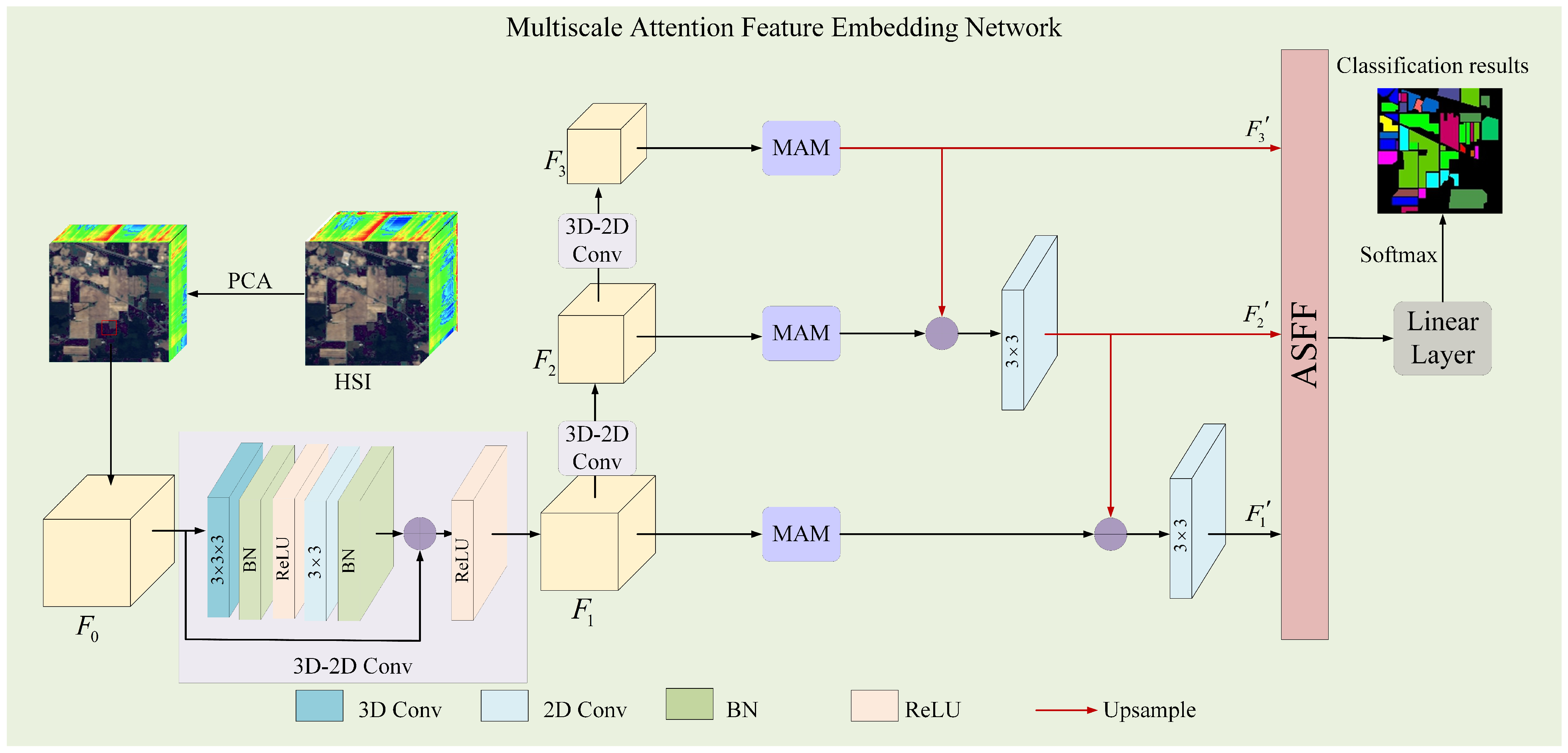
In this section, our proposed MAFEN for HSI classification is described in detail, and its overall framework is shown in Figure 1. Firstly, the MAFEN backbone network uses 3D-CNN and 2D-CNN to extract the features of different depths from the dimensionality-reduced hyperspectral images. Secondly, MAM was designed to enhance the representation ability of different levels of features through multiscale convolution, and the spectral–spatial attention mechanism was used to highlight important information and suppress redundant information. Then, the high-level semantic information was embedded into the low-level local spatial information through the top-down channel to make the features at different levels have rich semantics. Finally, ASFF was introduced to adaptively fuse the features of different levels to obtain the final feature representation for classification.

2.1. Multiscale Attention Module

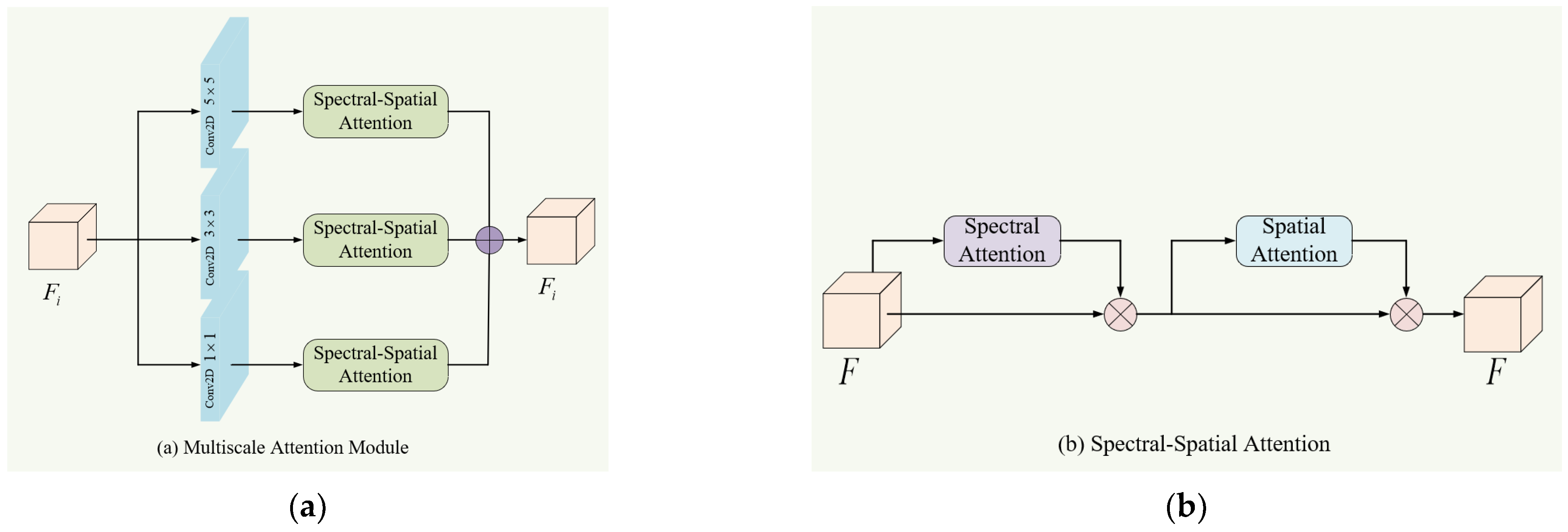
CNNs are limited by fixed-size receptive fields, which may result in insufficient local spatial features. To obtain richer local information of features at different levels, a multiscale approach can be used to control the sizes of convolutional kernels, thus obtaining different receptive fields. Moreover, the feature maps may contain redundant information that could degrade the representation performance, thereby affecting the final classification results. Therefore, we utilized spectral–spatial attention to extract crucial information from the features obtained using multiscale convolutions to enhance classification performance. We designed an MAM that utilized multiscale convolutions and spectral–spatial attention to obtain more rich and effective feature representations. Figure 2a,b illustrates the overall framework of the MAM and the structure of the spectral–spatial attention module, respectively, as described below.

As shown in Figure 2, firstly, the MAM convolved the features $F_i\left(i=1,2,3\right)$ of different levels with three convolutional kernels of different sizes to obtain multi-scale information, where the sizes of the convolutional kernels were $1\times 1$, $3\times 3$ and $5\times 5$, respectively, and $F_1$, $F_2$ and $F_3$ represent the extracted low-level, mid-level, and high-level features, respectively. Then, the spectral–spatial attention modules were employed to extract effective information from the features extracted by each convolutional kernel, where spectral attention and spatial attention were cascaded. Finally, the three features were fused by element-wise summation.

2.1.1. Spectral Attention

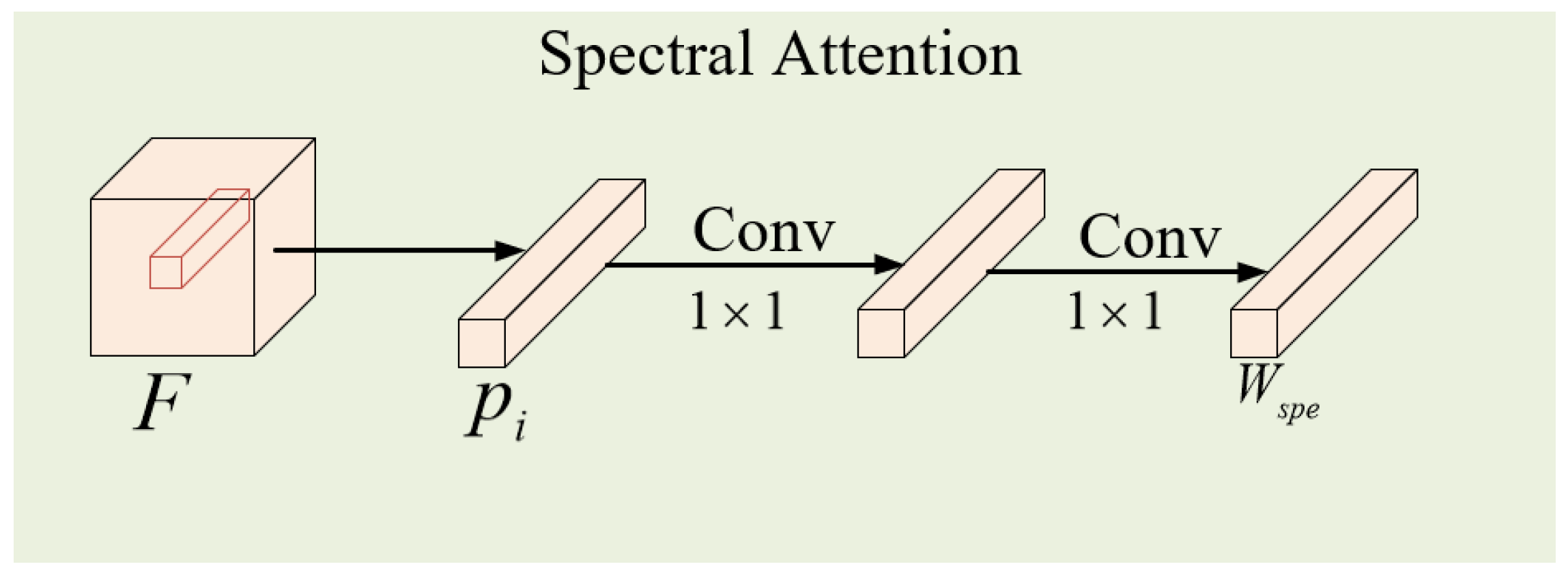
The main purpose of spectral attention is to generate band weights $W_{spe}$ to recalibrate the importance of each spectral band. Considering that the patch block may contain pixels from other classes, using global average pooling may introduce interference to the pixels of the current class. Therefore, we only used the center vector $p_i$ to generate the weight $W_{spe}$.

The specific structure of the spectral attention module is shown in Figure 3. Firstly, the center vector $p_i\in R^{1\times 1\times b}$ was taken from the input cube $F\in R^{s\times s\times b}$, where $s\times s$ was the spatial size of $F$ and $b$ was the number of bands. Then, the band weight $W_{spe}\in R^{1\times 1\times b}$ was obtained through the calculation of two convolutional layers with a kernel size of $1\times 1$, as shown in Equation (1).

$$W_{spe}=\sigma \left(W_2\ast \left(\delta \left(W_1\ast p_i\right)\right)\right),$$

(1)

where $\sigma$ and $\delta$ represent the sigmoid and ReLU activation functions, respectively. $W_1$ and $W_2$ are the weight parameters of the two convolutional layers, and $\ast$ represents the convolution operation. Finally, as shown in Figure 2b, the band weight $W_{spe}$ was used to recalibrate the bands in the feature $F$ to highlight the useful spectral information, using Equation (2).

$$F=W_{spe}\otimes F,$$

(2)

where $\otimes$ represents element-wise multiplication.

2.1.2. Spatial Attention

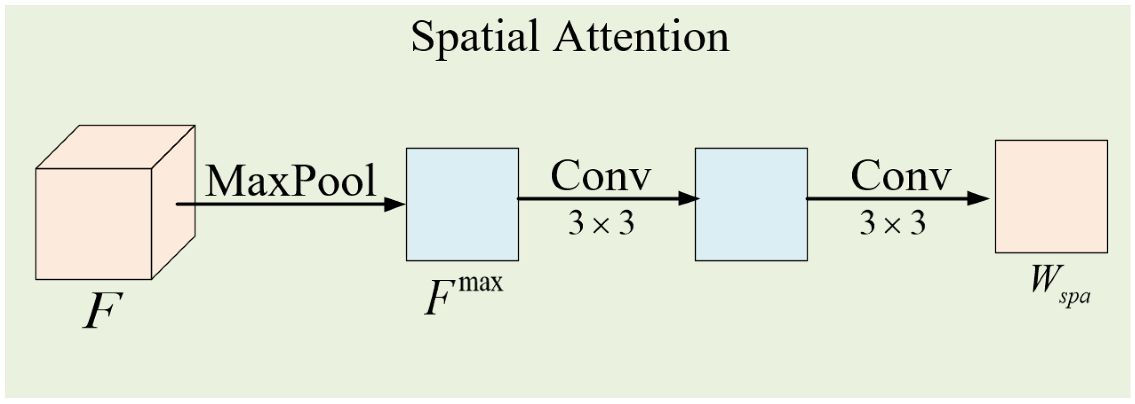
Spatial attention aims to enhance the spatial information for pixels belonging to the same class as that of the central pixel, while suppressing pixels of other classes. Therefore, the spatial weight $W_{spa}$ should have the same width and height as those of the input feature $F$, with a specific structure as shown in Figure 4. Firstly, global max pooling was applied to the input feature $F$ along the channel direction, as shown in Equation (3).

$$F^{\max }={\max }_c\left(F\left(i,j\right)\right),$$

(3)

where $F\left(i,j\right)$ represents the value at position $\left(i,j\right)$ in the feature $F\in R^{s\times s\times b}$, ${\max }_c$ represents taking the maximum value along the channel direction $c$ and $F^{\max }\in R^{s\times s}$ is the feature map after global max pooling. Then, it is passed through two 2D convolutional layers to generate the spatial weight $W_{spa}\in R^{s\times s}$, as shown in Equation (4).

$$W_{spa}=\sigma \left(\delta \left(F^{\max }\ast W_1\right)\ast W_2\right),$$

(4)

where $W_1$ and $W_2$ are the weight parameters of the two convolutional layers, $\sigma$ and $\delta$ represent the sigmoid and ReLU activation functions, respectively, and $\ast$ denotes the convolution operation. Finally, as shown in Figure 2b, the spatial weight $W_{spa}$ is used to recalibrate the spatial information in the feature $F$ and highlight the useful spatial information, using Equation (5).

$$F=W_{spa}\otimes F,$$

(5)

where $\otimes$ represents element-wise multiplication.

2.2. Feature Embedding Network

Deep neural networks learn the fine-grained features of local objects in HSIs in shallow layers, and high-level semantic features in deep layers. However, during the deep learning process, shallow features are often lost or even disappear, so they are generally not involved in the final HSI classification. In addition, different-depth features have different levels of information representation, and fully utilizing information at different levels is beneficial to improving the effectiveness of HSI classification. In this article, we propose a new Multiscale Attention Feature Embedding Network. The backbone of MAFEN consists of a spectral–spatial feature extraction channel and a deep feature embedding channel. The detailed description of the MAFEN is as follows.

Let $H\in R^{w\times h\times b}$ represent the original HSI data, where $w$ and $h$ represent the width and height of the spatial dimension, respectively, and $b$ is the number of spectral bands. Each pixel in $H$ corresponds to a one-hot label vector $Y\in R^{1\times 1\times K}$, where $K$ is the number of land cover classes. HSIs have rich spectral information, which will lead to a large number of spectral dimensions and an increase in computational complexity. HSIs may also contain noise, causing interference with the classification. Using Principal Component Analysis (PCA) to perform dimensionality reduction can improve classification accuracy by removing noise and redundant information, and can also reduce computation time and resource consumption, thereby enhancing computational efficiency and making deep learning models more efficient. Therefore, PCA is commonly used to process HSI data. PCA reduces the number of spectral bands from b to l, while maintaining the spatial size of HSI. The resulting reduced-dimensional HSI data are represented as $H_{pca}\in R^{w\times h\times l}$, where $l$ is the number of reduced spectral bands. To fully leverage the spectral and spatial information provided by the HSI, a set of cubes $F_0\in R^{s_0\times s_0\times l}$ is extracted from $H_{pca}$, where $s_0\times s_0$ represents the spatial size of the patch blocks in the HSI cube. The center pixel of each patch is denoted as $\left(x_i,y_i\right)$, and the true label of each patch is determined by the label of the center pixel.

(1) Feature Extraction Channel: Given the ith feature $F_i\in R^{s_i\times s_i\times l}$, i = 0, 1, 2, 3, where $F_0$ represents the cube corresponding to the HSI input data; $F_1$, $F_2$ and $F_3$ represent low-level, mid-level and high-level features, respectively. The feature map $F_{i+1}$ is obtained by applying two layers of convolutions (3D-CNN and 2D-CNN) and residual connections to each feature map $F_i$ in a bottom-up manner, as shown in Equations (6) and (7):

$$M=\delta \left(BN\left(f_1\left(F_i,w_1\right)\right)\right),$$

(6)

$$F_{i+1}=MP\left(\delta \left(BN\left(f_2\left(M,w_2\right)\right)+M\right)\right),$$

(7)

where $f_1\left(·,w_1\right)$ represents a 3D convolution with a weight parameter $w_1$ and kernel size of $3\times 3\times 3$, and $f_2\left(·,w_2\right)$ represents a 2D convolution with a weight parameter $w_2$ and kernel size of $3\times 3$. $BN$ stands for batch normalization, and $\delta$ represents the activation function, which is ReLU here. $MP\left(·\right)$ denotes the max pooling function.

The 3D-2D convolution is used to extract spectral–spatial features from the HSI data, resulting in three features with different levels of information. High-level features contain rich semantic information, while low-level features capture fine-grained local spatial information.

(2) Deep Feature Embedding Channel: Multiscale attention was applied to different deep features $F_i$ in three branches to extract effective spectral–spatial information, thereby enhancing the classification performance. Then, transpose convolution was applied to the deep features $F_i\left(i=3,2\right)$ to complete upsampling and obtain $F_i{}^{\prime }$, as shown in Equation (8).

$$F_i{}^{\prime }=\phi \left(F_i,\theta \right),$$

(8)

where $\phi \left(·,\theta \right)$ represents the transpose convolution with a kernel size of $3\times 3$ and weight parameter $\theta$. As a result, $F_i{}^{\prime }$ has the same spatial resolution as $F_{i-1}$. Next, $F_i{}^{\prime }$ and $F_{i-1}$ were added together for fusion, and the fused features were convolved as shown in Equation (9).

$$F_{i-1}{}^{\prime }=f_3\left(F_i{}^{\prime }\oplus F_{i-1},w_3\right),$$

(9)

where $f_3\left(·,w_3\right)$ represents the convolution operation with a weight parameter $w_3$, and $\oplus$ represents element-wise addition for fusion. Through the above process, high-level features can be embedded into low-level features, enhancing the feature representation capability of the model.

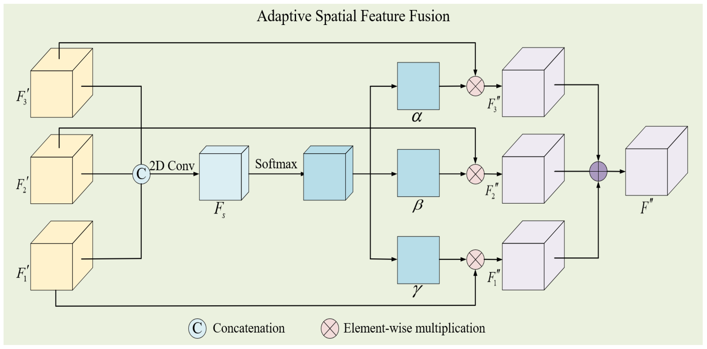
2.3. Adaptive Spatial Feature Fusion

In contrast to conventional feature fusion strategies, ASSF can learn the fusion weights for each feature map automatically through the network, achieving adaptive fusion. The specific structure is shown in Figure 5.

Firstly, the three different-level features $F_i{}^{\prime }\in R^{s\times s\times b},i=1,2,3$ were concatenated along the channel dimension to obtain the feature $F_s\in R^{s\times s\times 3b}$. Then, a convolution operation was applied to change the channel length, as shown in Equation (10).

$$F_s=\delta \left(f_4\left(F_s,w_4\right)\right),$$

(10)

where $f_4\left(·,w_4\right)$ represents a 2D convolution with a kernel size of $1\times 1$ and $\delta$ is the ReLU activation function. The resulting $F_s$ from the convolution operation has a size of $s\times s\times 3$. To obtain the feature fusion weights $\alpha ,\beta ,\gamma$ of size $s\times s$, the Softmax function was applied to normalize the exponential function of the data along the channel direction of $F_s$ at the same position, as shown in Equation (11).

$$\left[\alpha ,\beta ,\gamma \right]=\frac{\exp \left(F_{s,\left(i,j\right)}\left(k\right)\right)}{{\displaystyle {\sum }_{k=1}^3\exp \left(F_{s,\left(i,j\right)}\left(k\right)\right)}},$$

(11)

where $F_{s,\left(i,j\right)}\left(c\right)$ represents the value of the kth channel of the feature $F_s$ at position $\left(i,j\right)$. Therefore, the network can learn the weights for each feature automatically, enhancing the fusion capability. Next, features ${F_3}^{\prime }$, ${F_2}^{\prime }$ and ${F_1}^{\prime }$ were multiplied in an element-wise way by weights $\alpha$, $\beta$ and $\gamma$ in each band, respectively, to obtain ${F_3}^{″}$, ${F_2}^{″}$ and ${F_1}^{″}$, which were then summed to obtain the final feature representation $F^{″}$. Finally, the feature $F^{″}$ was fed into a linear layer for classification.

3. Experiment and Analysis

3.1. Dataset Description

In order to verify the performance of the proposed method, we selected four classical datasets for experiments, including Indian Pines, Kennedy Space Center (KSC), Pavia University and Salinas.

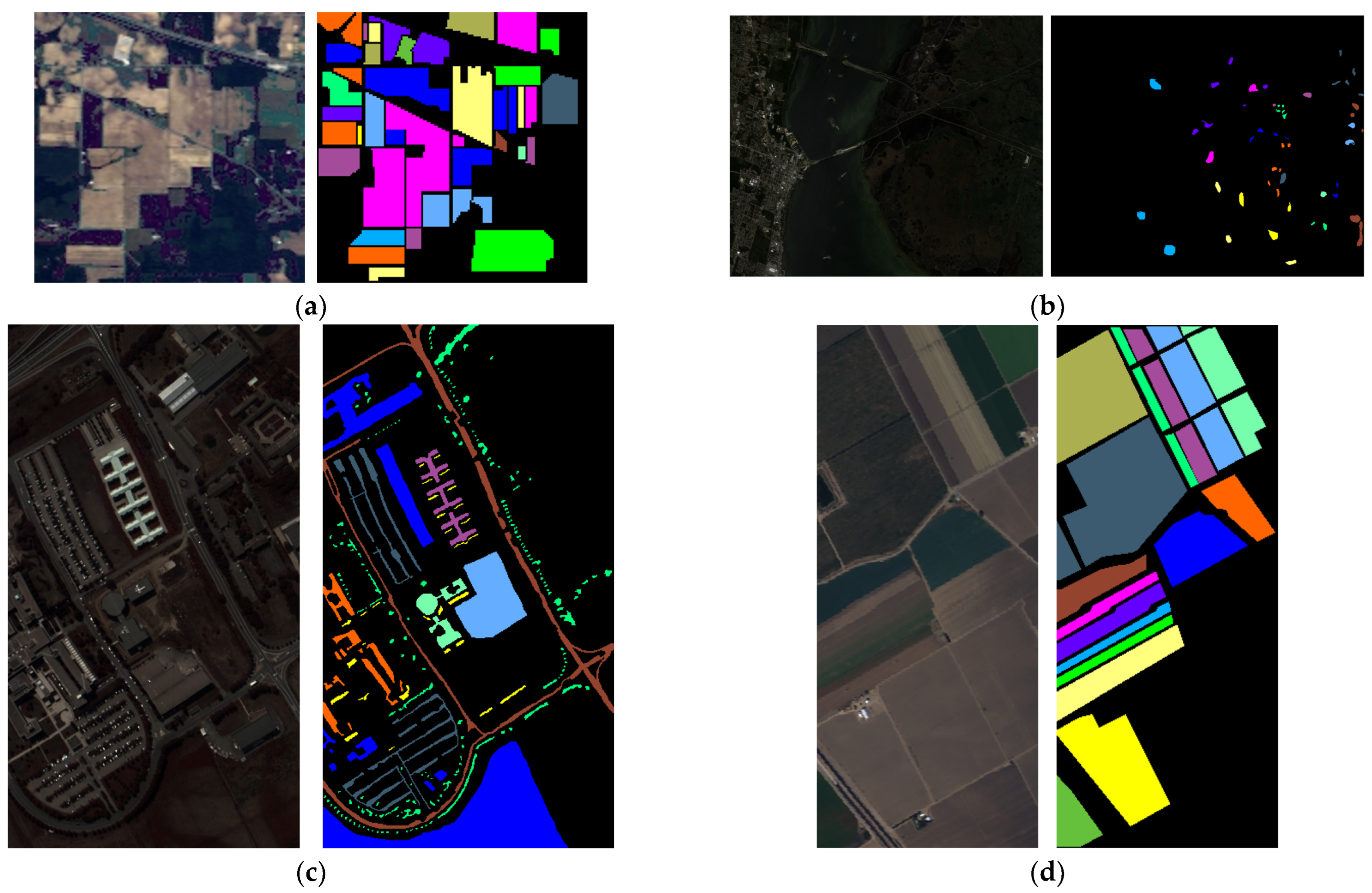
The Indian Pines dataset was a hyperspectral remote sensing image with a size of 145 × 145 and a spatial resolution of 20 m. It was acquired using an Airborne Visible/Infrared Imaging Spectrometer (AVIRIS). It contained 200 spectral bands and 16 land cover classes, for a total of 10,249 labeled samples. The false-color image and ground-truth label image are shown in Figure 6a.

Table 1. The information for each class in the Indian Pines dataset.

No.	Class	Color	Train	Test
1	Alfalfa		5	41
2	Corn-notill		143	1285
3	Corn-mintill		83	747
4	Corn		24	213
5	Grass-pasture		48	435
6	Grass-trees		73	657
7	Grass-pasture-mowed		3	25
8	Hay-windrowed		48	430
9	Oats		2	18
10	Soybean-notill		97	875
11	Soybean-mintill		245	2210
12	Soybean-clean		59	534
13	Wheat		20	185
14	Woods		126	1139
15	Buildings-Grass-Trees-Drives		39	347
16	Stone-Steel-Towers		9	84
Total			1024	9225

lists the specific classes of the Indian Pines dataset and the number of training and testing samples for each class.

The KSC dataset was a hyperspectral remote sensing image with a size of 512 × 217 and a spatial resolution of 18 m. It was also acquired using an AVIRIS sensor. It contained 176 spectral bands and 13 land cover classes, for a total of 5211 labeled samples. The false-color image and ground-truth label image are shown in Figure 6b.

Table 2. The information for each class in the KSC dataset.

No.	Class	Color	Train	Test
1	Scrub		76	685
2	Willow_swamp		24	219
3	CP_hammock		26	230
4	CP/Oak		25	227
5	Slash_pine		16	145
6	Oak/Broadleaf		23	206
7	Hardwood_swamp		10	95
8	Graminoid_marsh		43	388
9	Spartina_marsh		52	468
10	Catial_marsh		40	364
11	Salt_marsh		42	377
12	Mud_flats		50	453
13	Water		93	834
Total			520	4691

lists the specific classes of the KSC dataset and the number of training and testing samples for each class.

The Pavia University dataset was a hyperspectral remote sensing image with a size of 610 × 340 and a spatial resolution of 1.3 m. It was acquired using a Reflective Optics System Imaging Spectrometer (ROSIS). It contained 103 spectral bands and 9 land cover classes, for a total of 42,776 labeled samples. The false-color image and ground-truth label image are shown in Figure 6c.

Table 3. The information for each class in the Pavia University dataset.

No.	Class	Color	Train	Test
1	Asphalt		199	6432
2	Meadows		559	18,090
3	Gravel		63	2036
4	Trees		92	2972
5	Metal Sheets		40	1305
6	Bare soil		151	4878
7	Bitumen		40	1290
8	Bricks		110	3572
9	Shadows		28	919
Total			1282	41,494

lists the specific classes of the Pavia University dataset and the number of training and testing samples for each class.

The Salinas dataset was a hyperspectral remote sensing image with a size of 512 × 217 and a spatial resolution of 3.7 m. It was also acquired using an AVIRIS sensor. It contained 204 spectral bands and 16 land cover classes, for a total of 54,129 labeled samples. The false-color image and ground-truth label image are shown in Figure 6d.

Table 4. The information for each class in the Salinas dataset.

No.	Class	Color	Train	Test
1	Brocoli_green_weeds_1		60	1949
2	Brocoli_green_weeds_2		112	3614
3	Fallow		59	1917
4	Fallow_rough_plow		42	1352
5	Fallow_smooth		80	2598
6	Stubble		119	3840
7	Celery		107	3472
8	Grapes_untrained		338	10,933
9	Soil_vinyard_develop		186	6017
10	Corn_senesced_green_weeds		98	3180
11	Lettuce_romaine_4wk		32	1036
12	Lettuce_romaine_5wk		58	1869
13	Lettuce_romaine_6wk		27	889
14	Lettuce_romaine_7wk		32	1038
15	Vinyard_untrained		218	7050
16	Vinyard_vertical_trellis		54	1753
Total			1622	52,507

lists the specific classes of the Salinas dataset and the number of training and testing samples for each class.

3.2. Experimental Setting

(1) Evaluation Metrics: To quantitatively assess the effectiveness of the proposed model, we used Overall Accuracy (OA), Average Accuracy (AA) and the Kappa coefficient as the evaluation metrics. A higher value for each metric indicated better classification performance.

(2) Configuration: The experiments were conducted using an Inter Xeon Silver 4114 2.2 GHz CPU, 128 GB RAM, and a NVIDIA Geforce RTX 2080 Ti 12 GB graphics card. The PyTorch deep learning framework was used to train the network, with epoch and batch_size set to 100 and 32, respectively. A learning rate decay strategy was employed, with an initial learning rate of 0.001, and a decay of 0.1 every 50 epochs. Adam was chosen as the optimization method for the experiments. Each method was tested five times, and the mean value was taken as the experimental result, along with the calculation of the standard deviation.

In the Indian Pines, Pavia University and Salinas datasets, the size of the patch block (Patch_Size) was set to 13, while in the KSC dataset it was set to 15. The dimension of PCA dimensionality reduction (PCA_Components) was set to 64, 128, 32 and 96 for the Indian Pines, KSC, Pavia University and Salinas datasets, respectively.

In practice, labeling samples of hyperspectral image data requires expert knowledge, which is time-consuming and expensive. Therefore, how to train the model well with a limited or low percentage of samples has become an important topic [17], and it is also a necessary way to test the effectiveness of the proposed model. In recent years, with the improvement of deep neural network models, the percentage of the training samples has tended to decrease from 30% [24] to 10%, 5% or 3% [17,20]. In this paper, we also used a low percentage of samples to train the proposed model. There were many available samples in the Pavia University and Salinas datasets, so the number of random training samples in these two datasets accounted for 3% of the total samples, and the number of random training samples in the Indian Pines and KSC datasets accounted for 10% of the total samples.

3.3. Experimental Results and Analysis

3.3.1. Classification Results

We compared the proposed MAFEN model with several representative methods to validate its effectiveness, including traditional methods such as SVM, deep-learning-based methods such as 3DCNN [22], SSRN [23], DFFN [30] and HybridSN [24], as well as attention-based methods such as Speformer [36] and SSFTT [37]. The detailed experimental results of these methods on the Indian Pines, KSC, Pavia University and Salinas datasets are as follows.

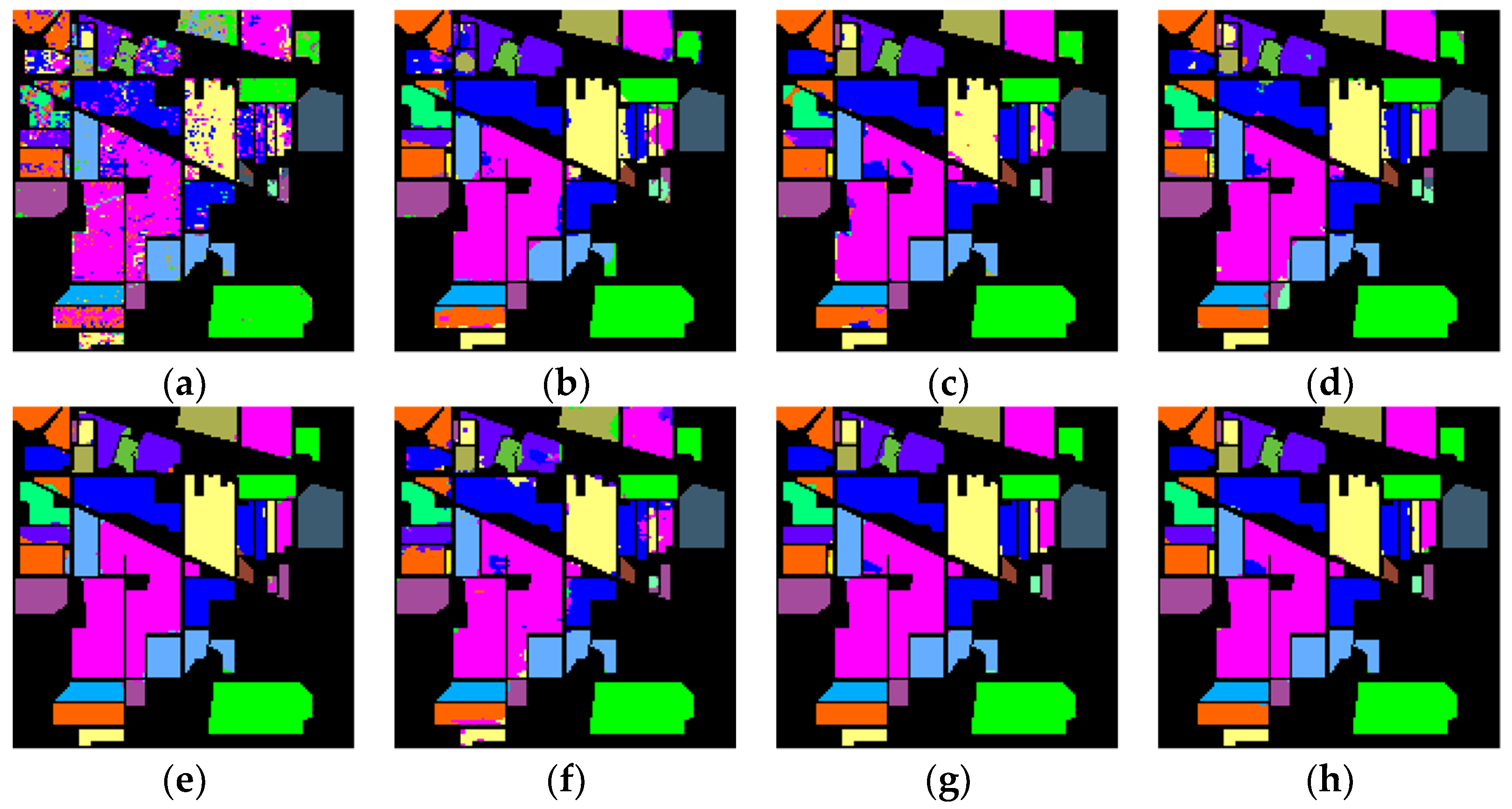
(1) Indian Pines: Firstly, all the models were evaluated using the Indian Pines dataset, and the quantitative experimental results are shown in

Table 5. Classification results of different methods on the Indian Pines dataset.

Class	SVM	3DCNN	SSRN	DFFN	HybridSN	Speformer	SSFTT	MAFEN
1	33.81 ± 0.05	89.74 ± 0.01	96.58 ± 4.78	91.16 ± 0.06	90.73 ± 13.83	94.63 ± 5.21	97.07 ± 3.58	100 ± 0.00
2	74.99 ± 0.03	85.01 ± 0.12	93.87 ± 2.94	93.47 ± 0.04	93.96 ± 1.88	89.90 ± 1.71	96.68 ± 0.68	96.76 ± 0.56
3	68.86 ± 0.02	86.41 ± 0.26	93.95 ± 4.99	89.12 ± 0.14	98.90 ± 0.67	89.97 ± 1.25	99.22 ± 0.41	99.57 ± 0.66
4	47.57 ± 0.04	96.19 ± 0.02	86.29 ± 2.17	92.41 ± 0.05	96.53 ± 2.23	97.65 ± 1.07	99.62 ± 0.55	99.15 ± 0.91
5	85.29 ± 0.03	88.19 ± 0.01	99.17 ± 0.78	81.38 ± 0.06	98.85 ± 1.32	97.06 ± 1.07	98.57 ± 1.48	99.86 ± 0.11
6	95.77 ± 0.03	88.16 ± 0.02	98.14 ± 0.50	96.53 ± 0.01	98.99 ± 0.67	99.33 ± 0.41	99.63 ± 0.39	99.51 ± 0.34
7	60.00 ± 0.24	87.50 ± 0.04	97.6 ± 3.20	93.60 ± 0.08	18.4 ± 36.8	71.20 ± 10.24	100 ± 0.00	100 ± 0.00
8	98.56 ± 0.01	100 ± 0.00	99.58 ± 0.45	100 ± 0.00	99.91 ± 0.19	99.86 ± 0.19	100 ± 0.00	99.90 ± 0.19
9	30.00 ± 0.08	88.23 ± 0.16	88.89 ± 7.03	66.67 ± 0.12	21.43 ± 7.36	66.67 ± 11.11	76.67 ± 7.36	93.34 ± 5.44
10	75.45 ± 0.02	89.35 ± 0.01	96.32 ± 1.88	89.86 ± 0.05	99.11 ± 0.15	92.78 ± 1.41	97.76 ± 1.12	99.43 ± 0.19
11	82.14 ± 0.01	93.71 ± 0.03	94.14 ± 3.04	89.69 ± 0.14	99.36 ± 0.25	95.70 ± 1.34	99.38 ± 0.33	99.38 ± 0.20
12	61.31 ± 0.01	93.63 ± 0.23	92.77 ± 2.25	77.21 ± 0.14	95.43 ± 1.39	80.56 ± 3.29	96.29 ± 1.36	98.58 ± 0.39
13	95.14 ± 0.02	100 ± 0.00	99.68 ± 0.65	95.19 ± 0.03	98.38 ± 1.41	99.68 ± 0.43	98.16 ± 2.04	99.89 ± 0.22
14	94.19 ± 0.02	97.99 ± 0.04	99.37 ± 0.13	97.76 ± 0.01	99.39 ± 0.52	98.53 ± 1.03	99.89 ± 0.21	99.84 ± 0.13
15	53.91 ± 0.04	88.92 ± 0.01	97.64 ± 1.05	94.30 ± 0.02	99.08 ± 1.05	90.72 ± 2.67	97.46 ± 2.90	100 ± 0.00
16	80.95 ± 0.05	95.29 ± 0.01	99.28 ± 0.95	98.05 ± 0.01	96.90 ± 1.78	91.90 ± 5.80	88.80 ± 6.80	97.14 ± 0.95
OA	79.60 ± 0.01	91.62 ± 0.01	95.75 ± 0.61	91.43 ± 0.04	97.73 ± 0.33	93.92 ± 0.91	98.49 ± 0.46	99.10 ± 0.06
AA	71.12 ± 0.01	91.78 ± 0.01	95.83 ± 0.61	90.40 ± 0.04	86.49 ± 0.33	91.01 ± 0.93	96.58 ± 0.46	98.90 ± 0.30
Kappa	76.66 ± 0.01	90.45 ± 0.01	95.16 ± 0.61	90.27 ± 0.04	97.41 ± 0.33	93.06 ± 1.04	98.28 ± 0.46	98.98 ± 0.07

, where the numbers in bold mean the best results. The results of evaluation metrics show that the proposed MAFEN method performed the best, obtaining the highest OA, AA and Kappa values. Specifically, compared with SVM, the accuracy of 3DCNN was improved by 12.02%, which shows that deep learning has a significant advantage in HSI classification. SSRN had better classification performance than 3DCNN because it uses continuous residual blocks to learn spectral and spatial features separately. The classification performance of DFFN was lower than that of SSRN, which may be because the feature distribution of the Indian Pines dataset did not match well with the DFFN network structure and the way of feature fusion. The poor accuracy of HybridSN and Speformer in the “Grass-pawn-mowed” (class 7, mint green) and “Oats” (class 9, yellow) categories was due to the fact that the number of training samples in the two categories was only three and two, respectively, which was challenging for HSI classification. SSFTT achieved 100% accuracy in the “Grass-Pasture-Mowed” category, but 76.67% accuracy in the “Oats” category, because the region shape of this category was narrow and spatial features could not be fully extracted. However, the accuracy of the proposed model on the two categories was 100% and 93.34%, respectively, and the accuracy of each category was relatively close, which indicates that the model has good feature expression ability for samples with a small training number and an irregular region shape.

Figure 7 shows the classification maps of these methods on the Indian Pines dataset. The compared methods performed poorly on the land cover objects with region edges and narrow shapes, but the proposed MAFEN model generated more accurate classification maps with better homogeneity in each region. This is because MAFEN enhances the feature representation of different categories through deep feature embedding and multiscale attention learning.

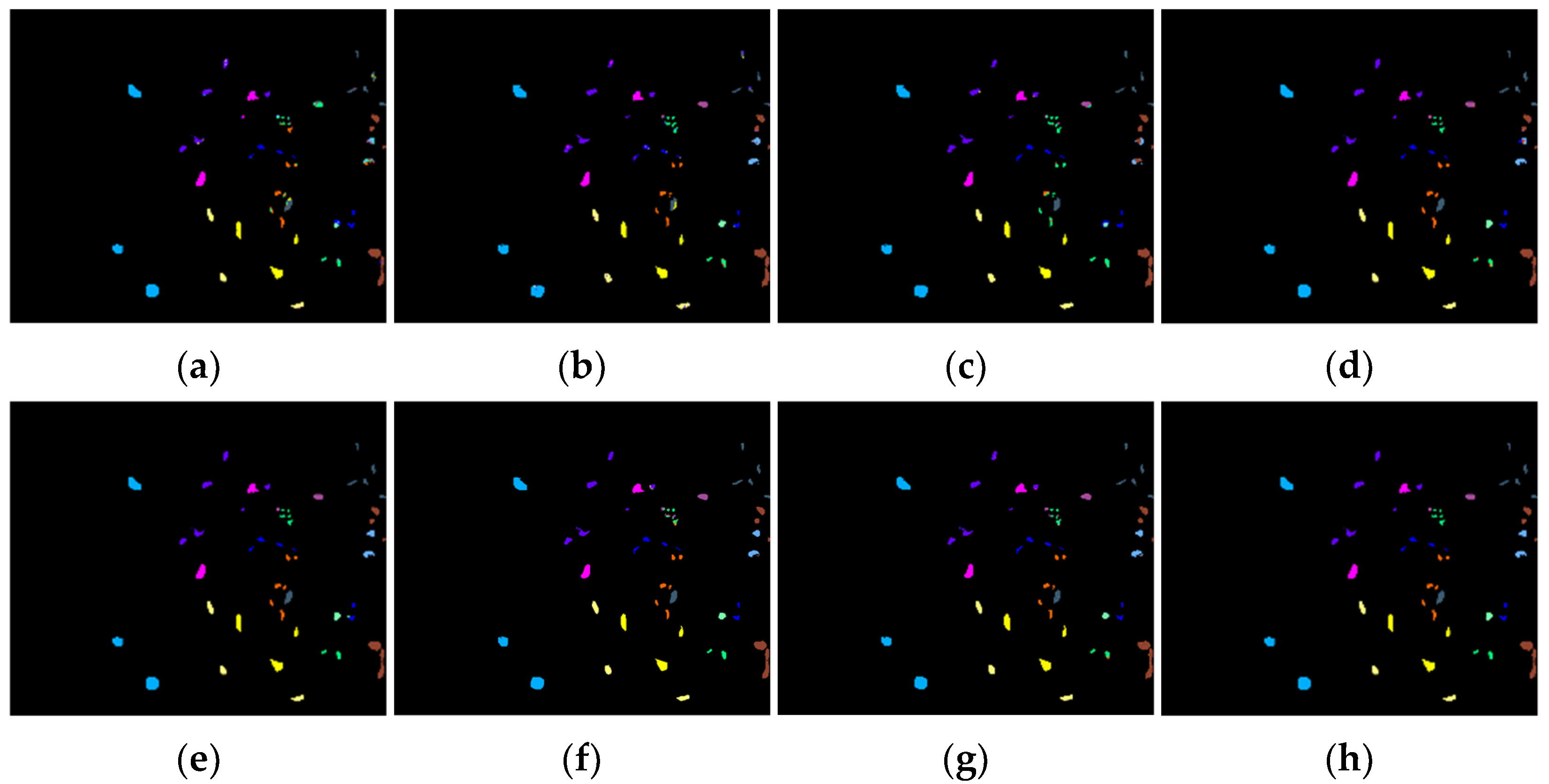
(2) KSC: Secondly, we evaluated all the models on the KSC dataset, and the quantitative experimental results are shown in

Table 6. Classification results of different methods on the KSC dataset.

Class	SVM	3DCNN	SSRN	DFFN	HybridSN	Speformer	SSFTT	MAFEN
1	95.01 ± 0.01	98.12 ± 0.34	99.68 ± 0.35	99.74 ± 0.21	100 ± 0.00	99.74 ± 0.06	99.80 ± 0.25	100 ± 0.00
2	85.84 ± 0.06	77.53 ± 8.56	98.54 ± 0.73	99.27 ± 1.07	97.35 ± 1.27	98.36 ± 0.89	100 ± 0.00	100 ± 0.00
3	86.93 ± 0.04	87.15 ± 4.09	70.78 ± 32.36	97.22 ± 2.26	98.43 ± 1.66	97.13 ± 2.05	100 ± 0.00	99.74 ± 0.35
4	50.66 ± 0.03	80.11 ± 1.30	82.91 ± 11.67	83.96 ± 7.69	95.51 ± 2.42	70.84 ± 2.29	91.37 ± 6.85	98.68 ± 1.47
5	31.45 ± 0.19	84.25 ± 6.46	72.28 ± 34.09	91.31 ± 0.94	97.93 ± 1.57	94.07 ± 2.81	100 ± 0.00	100 ± 0.00
6	52.75 ± 0.04	87.63 ± 4.32	77.57 ± 19.72	75.92 ± 6.51	98.64 ± 1.77	92.23 ± 1.62	99.51 ± 0.75	100 ± 0.00
7	75.16 ± 0.16	96.22 ± 4.05	69.57 ± 36.19	100 ± 0.00	80.00 ± 8.52	100 ± 0.00	100 ± 0.00	100 ± 0.00
8	89.28 ± 0.03	85.83 ± 3.65	99.48 ± 0.36	99.43 ± 0.50	100 ± 0.00	99.95 ± 0.10	100 ± 0.00	100 ± 0.00
9	97.73 ± 0.01	95.77 ± 0.90	100 ± 0.00	98.50 ± 0.63	100 ± 0.00	100 ± 0.00	100 ± 0.00	100 ± 0.00
10	94.51 ± 0.02	93.43 ± 4.76	99.78 ± 0.44	99.89 ± 0.22	99.07 ± 1.87	99.67 ± 0.32	100 ± 0.00	100 ± 0.00
11	97.04 ± 0.01	93.86 ± 2.54	100 ± 0.00	99.63 ± 0.27	99.95 ± 0.11	99.95 ± 0.11	100 ± 0.00	99.84 ± 0.32
12	88.30 ± 0.04	95.74 ± 1.39	99.25 ± 0.38	99.38 ± 0.61	100 ± 0.00	93.55 ± 2.80	99.51 ± 0.87	100 ± 0.00
13	99.07 ± 0.01	98.67 ± 1.07	100 ± 0.00	100 ± 0.00	100 ± 0.00	100 ± 0.00	100 ± 0.00	100 ± 0.00
OA	87.81 ± 0.01	92.74 ± 1.42	95.04 ± 3.31	97.39 ± 0.62	98.98 ± 0.91	97.15 ± 0.40	99.48 ± 0.43	99.91 ± 0.09
AA	80.29 ± 0.01	90.33 ± 1.46	89.99 ± 7.71	95.71 ± 0.99	97.45 ± 3.23	95.81 ± 0.50	99.25 ± 0.64	99.87 ± 0.14
Kappa	86.41 ± 0.01	91.91 ± 1.58	94.47 ± 3.70	97.10 ± 0.69	98.86 ± 1.02	96.83 ± 0.45	99.43 ± 0.48	99.90 ± 0.10

. The KSC dataset had a sparse distribution of classes, and patches were less affected by interference from neighboring classes, which allowed for better extraction of pixel-level features. Therefore, the accuracy of various methods was relatively high. Among them, HybridSN and Speformer achieved 100% accuracy in five and three categories, respectively, and SSFTT achieved 100% accuracy in nine classes. The proposed MAFEN model achieved 100% accuracy in 10 classes, with OA, AA and Kappa values reaching 99.91%, 99.87% and 99.90%, respectively.

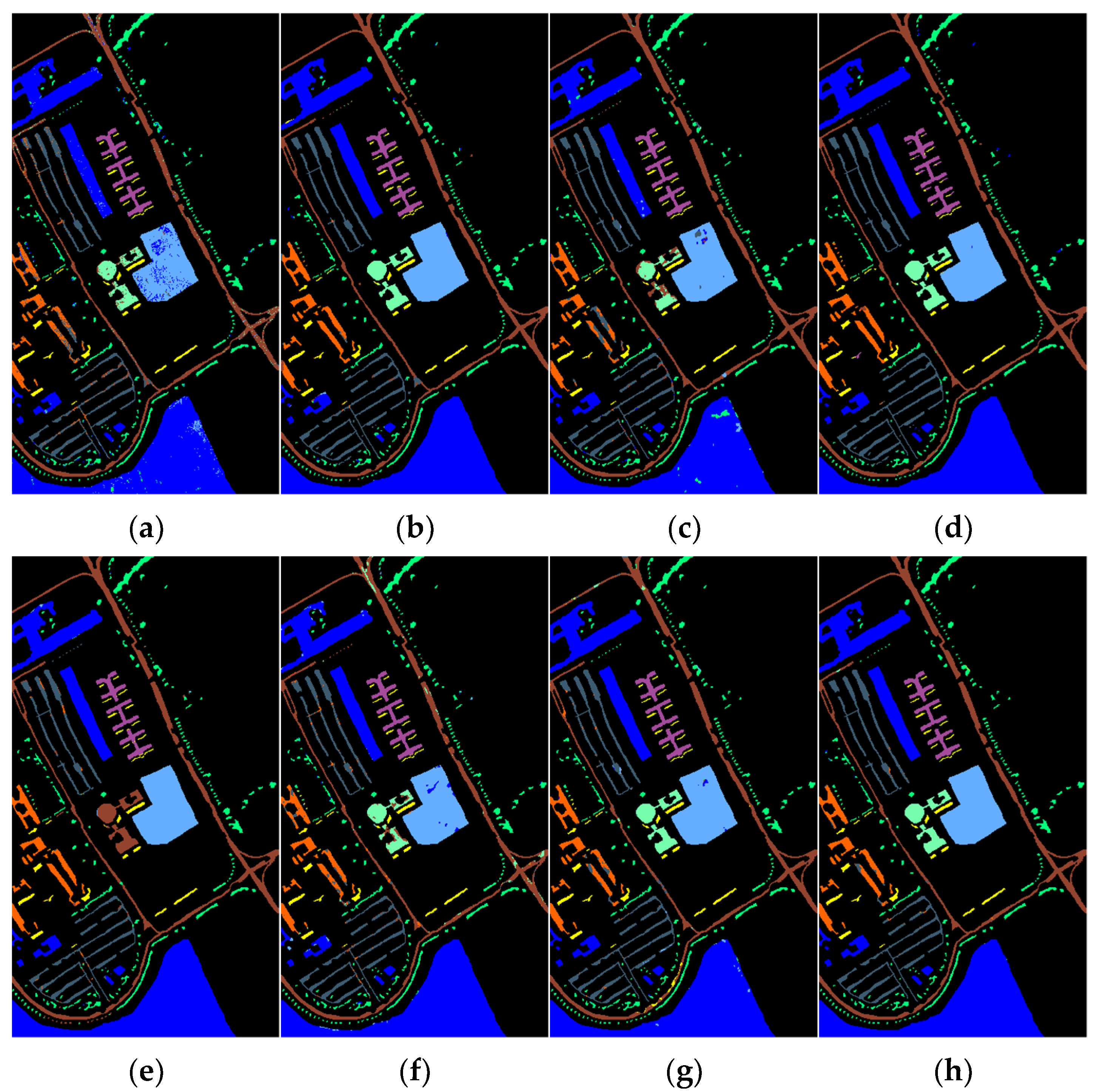
Figure 8 displays the classification maps of these methods on the KSC dataset. Several comparison methods had more noise points in the category “CP/Oak” (class 4, in cyan), which led to poor classification results. Among them, HybridSN achieved the best classification performance, reaching 95.51%. The proposed MAFEN model can better distinguish this category and achieved the best accuracy in this category, reaching 98.68%.

(3) Pavia University: We further evaluated all the models on the Pavia University dataset, and the quantitative experimental results are shown in

Table 7. Classification results of different methods on the Pavia University dataset.

Class	SVM	3DCNN	SSRN	DFFN	HybridSN	Speformer	SSFTT	MAFEN
1	94.65 ± 0.01	98.75 ± 0.01	95.04 ± 2.61	99.36 ± 0.47	97.33 ± 4.49	93.59 ± 0.50	97.58 ± 1.50	99.29 ± 0.56
2	98.12 ± 0.01	99.35 ± 0.01	99.49 ± 0.59	99.96 ± 0.03	99.90 ± 0.05	99.29 ± 0.16	99.67 ± 0.08	99.97 ± 0.02
3	76.84 ± 0.04	91.83 ± 0.03	86.31 ± 6.14	97.89 ± 1.05	98.57 ± 0.79	87.65 ± 2.41	90.27 ± 3.54	91.68 ± 2.31
4	92.91 ± 0.03	93.00 ± 0.02	96.52 ± 0.85	90.51 ± 3.52	95.38 ± 1.03	95.34 ± 0.32	97.19 ± 1.14	98.48 ± 0.64
5	99.30 ± 0.01	98.57 ± 0.01	98.74 ± 1.54	96.88 ± 3.45	98.57 ± 0.90	99.97 ± 0.06	99.91 ± 0.15	100 ± 0.00
6	87.84 ± 0.02	99.68 ± 0.01	91.96 ± 4.58	99.40 ± 0.45	100 ± 0.00	96.87 ± 0.45	98.43 ± 1.15	99.79 ± 0.27
7	85.92 ± 0.02	99.70 ± 0.01	85.44 ± 12.85	99.18 ± 0.76	59.94 ± 5.94	83.16 ± 1.39	97.72 ± 1.31	98.60 ± 1.08
8	89.92 ± 0.01	96.56 ± 0.02	90.09 ± 5.72	97.99 ± 1.72	95.74 ± 3.04	93.51 ± 0.53	97.22 ± 0.94	97.87 ± 0.63
9	99.76 ± 0.01	93.65 ± 0.03	98.48 ± 1.22	78.24 ± 12.68	94.04 ± 3.03	98.74 ± 0.56	97.91 ± 2.61	99.41 ± 0.47
OA	93.94 ± 0.01	98.09 ± 0.01	95.76 ± 0.58	98.25 ± 0.42	97.35 ± 1.62	96.28 ± 0.16	98.26 ± 0.26	99.09 ± 0.03
AA	91.69 ± 0.01	96.79 ± 0.01	93.56 ± 0.87	95.49 ± 1.44	93.28 ± 5.22	94.24 ± 0.26	97.32 ± 0.49	98.34 ± 0.18
Kappa	91.93 ± 0.01	97.47 ± 0.01	94.37 ± 0.78	97.68 ± 0.57	96.48 ± 2.16	95.07 ± 0.21	97.69 ± 0.34	98.80 ± 0.05

. The Pavia University dataset had a large number of samples in each category and abundant training samples, resulting in good classification performance for all methods. Compared with other methods, the proposed MAFEN model achieved the best overall classification results and the best accuracy in most categories.

Figure 9 shows the classification maps of these methods on the Pavia University dataset. The “Gravel” (class 3, in orange) and “Bricks” (class 8, in steel blue) classes had similar spectra but differed in spatial details. From the classification maps, it can be seen that SSRN using deep features for classification could not effectively distinguish “Gravel” and “Bricks”. However, the proposed model performed well on “Gravel” and “Bricks”, which indicates that utilizing shallow local spatial details was beneficial for distinguishing the “Gravel” and “Bricks” classes.

(4) Salinas: Finally, we evaluated all the models on the Salinas dataset, and quantitative analysis results for different methods are presented in

Table 8. Classification results of different methods on the Salinas dataset.

Class	SVM	3DCNN	SSRN	DFFN	HybridSN	Speformer	SSFTT	MAFEN
1	99.35 ± 0.01	99.96 ± 0.01	99.64 ± 0.30	97.98 ± 4.04	99.94 ± 0.12	99.68 ± 0.53	99.99 ± 0.02	100 ± 0.00
2	99.88 ± 0.01	99.52 ± 0.01	100 ± 0.00	99.62 ± 0.22	100 ± 0.00	99.75 ± 0.23	99.99 ± 0.01	99.99 ± 0.02
3	99.12 ± 0.01	98.37 ± 0.01	99.99 ± 0.02	99.99 ± 0.02	100 ± 0.00	98.41 ± 0.90	99.97 ± 0.04	100 ± 0.00
4	99.74 ± 0.01	95.63 ± 0.02	98.79 ± 0.91	91.72 ± 8.36	99.87 ± 0.12	99.56 ± 0.25	99.62 ± 0.20	99.50 ± 0.35
5	98.11 ± 0.01	99.11 ± 0.01	99.69 ± 0.34	99.85 ± 0.29	99.71 ± 0.43	99.41 ± 0.25	99.68 ± 0.24	99.73 ± 0.44
6	99.96 ± 0.01	100 ± 0.00	99.83 ± 0.33	98.68 ± 1.88	99.99 ± 0.01	99.98 ± 0.02	99.98 ± 0.04	99.99 ± 0.02
7	99.85 ± 0.01	99.94 ± 0.01	99.85 ± 0.14	99.83 ± 0.07	99.95 ± 0.09	99.37 ± 0.49	99.95 ± 0.04	100 ± 0.00
8	90.83 ± 0.01	94.36 ± 0.02	91.89 ± 6.05	99.08 ± 1.71	99.92 ± 0.12	97.77 ± 0.34	96.81 ± 1.11	99.81 ± 0.15
9	99.75 ± 0.01	99.74 ± 0.01	100 ± 0.00	100 ± 0.00	100 ± 0.00	99.18 ± 0.30	99.97 ± 0.06	100 ± 0.00
10	96.17 ± 0.01	98.38 ± 0.01	97.73 ± 1.11	100 ± 0.00	99.84 ± 0.16	99.53 ± 0.24	99.36 ± 0.35	99.97 ± 0.05
11	96.12 ± 0.02	98.01 ± 0.01	99.52 ± 0.45	99.71 ± 0.48	100 ± 0.00	99.15 ± 0.32	99.86 ± 0.08	100 ± 0.00
12	100 ± 0.00	99.92 ± 0.01	100 ± 0.00	97.15 ± 1.66	99.65 ± 0.70	99.05 ± 0.90	99.84 ± 0.32	100 ± 0.00
13	98.88 ± 0.01	99.52 ± 0.01	99.73 ± 0.54	97.16 ± 1.97	39.29 ± 4.85	98.90 ± 0.44	98.81 ± 0.69	99.91 ± 0.08
14	94.31 ± 0.02	95.87 ± 0.01	95.16 ± 3.96	93.47 ± 6.03	96.95 ± 5.82	96.59 ± 1.77	98.88 ± 0.16	98.92 ± 0.38
15	69.37 ± 0.03	87.70 ± 0.05	87.48 ± 6.68	97.57 ± 2.63	97.10 ± 5.19	95.53 ± 0.62	97.83 ± 0.41	99.43 ± 0.24
16	98.95 ± 0.01	99.49 ± 0.01	99.16 ± 0.38	100 ± 0.00	99.93 ± 0.14	99.60 ± 0.28	99.27 ± 0.19	99.54 ± 0.26
OA	93.30 ± 0.01	96.64 ± 0.01	96.27 ± 0.54	98.77 ± 0.69	98.46 ± 1.19	98.49 ± 0.12	98.89 ± 0.28	99.82 ± 0.06
AA	96.27 ± 0.01	97.84 ± 0.01	98.03 ± 0.28	98.24 ± 0.85	95.76 ± 2.91	98.84 ± 0.21	99.36 ± 0.13	99.80 ± 0.04
Kappa	92.52 ± 0.01	96.26 ± 0.01	95.85 ± 0.59	98.63 ± 0.77	98.28 ± 1.33	98.32 ± 0.13	98.77 ± 0.31	99.80 ± 0.07

. The Salinas dataset had larger regions and regular shapes for different classes, which allowed for better extraction of spatial features. The proposed MAFEN model achieved an accuracy of 100% for six classes, with OA, AA and Kappa values reaching 99.82%, 99.80% and 99.80%, respectively. This further confirms the feature representation capability of the proposed model.

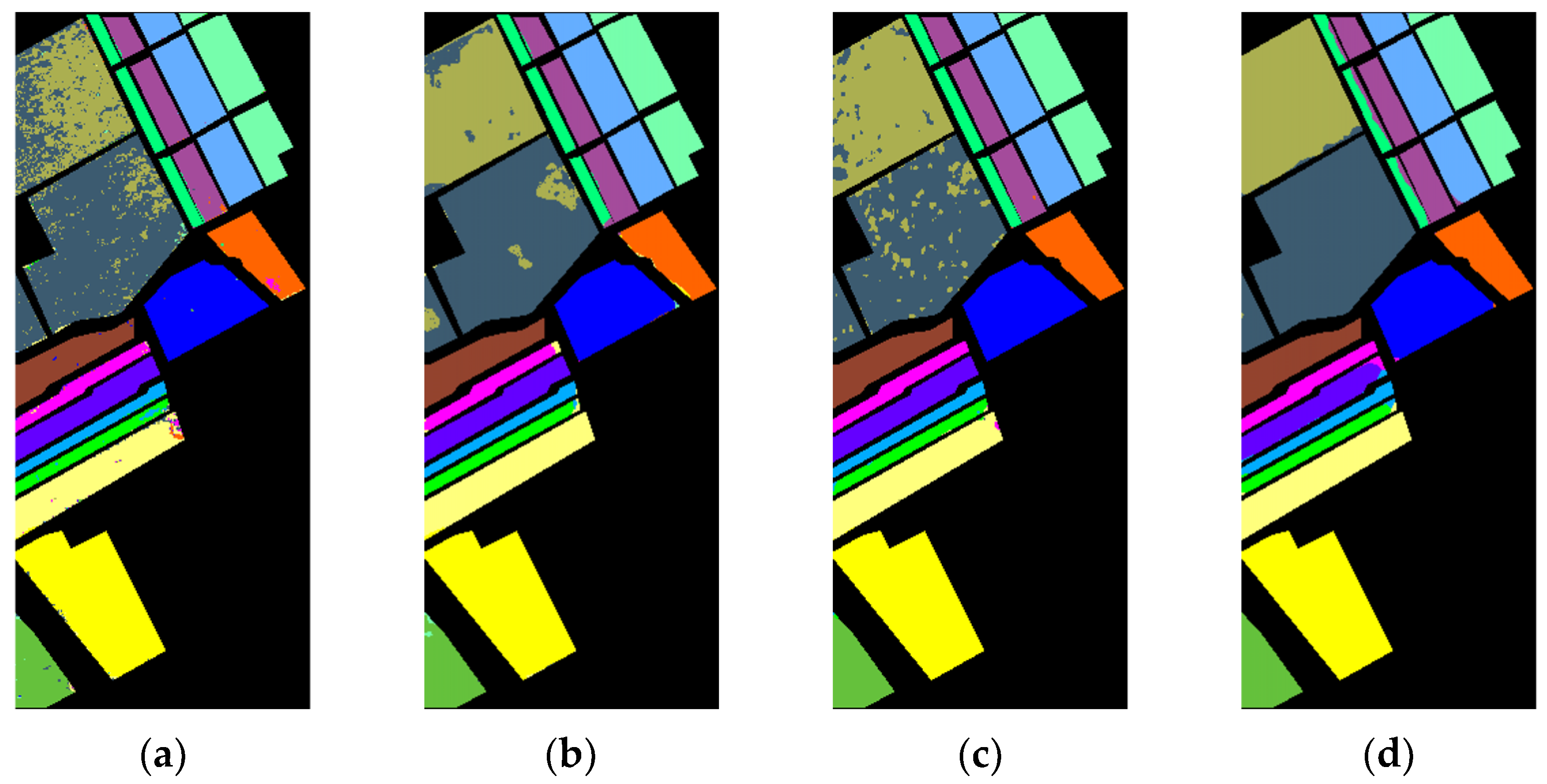
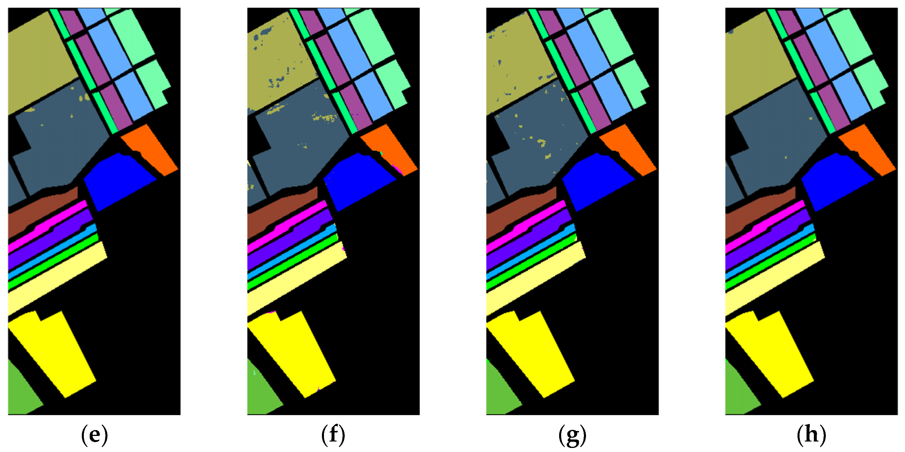
Figure 10 shows the classification maps of different methods on the Salinas dataset. From the top left corner of the classification maps, we can observe that due to the very similar spectra of “Grapes Untrained” (class 8, in steel blue) and “Vinyard Untrained” (class 15, in olive), the compared methods contained a lot of noise in the classification maps of these two classes. However, the proposed MAFEN model, which has better spectral–spatial feature representation capability, was able to distinguish these two classes, resulting in smoother and more accurate classification maps.

3.3.2. Parameter Analysis

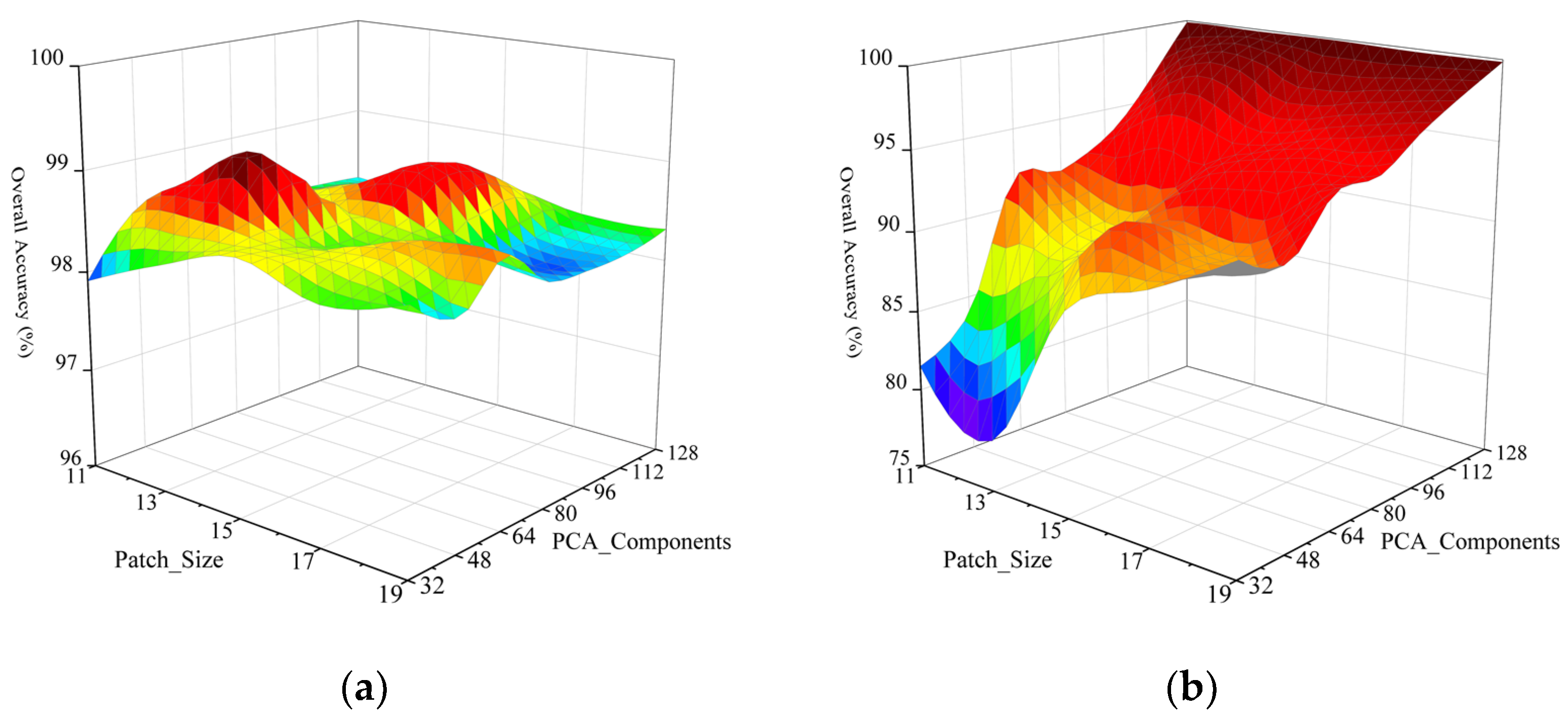
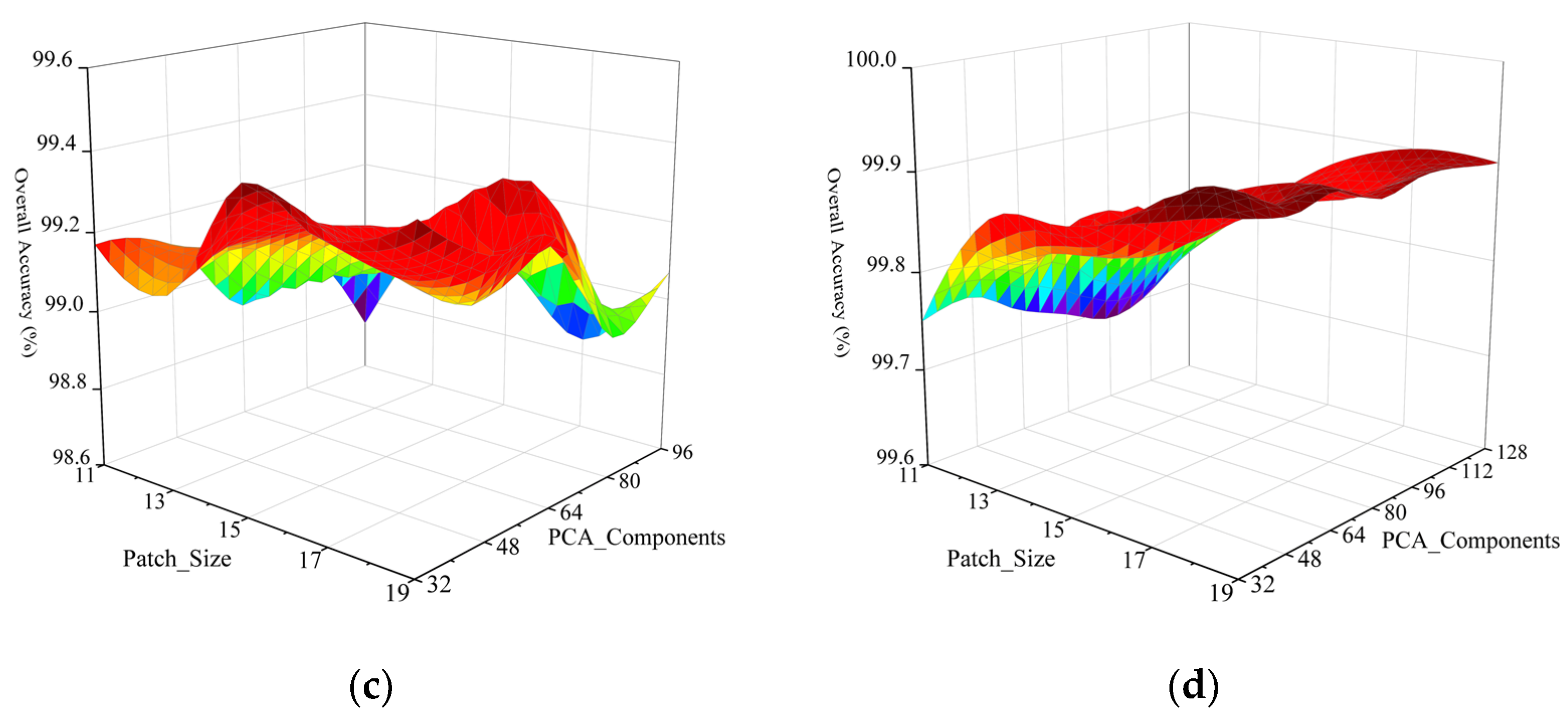
(1) Impact of Patch_Size and PCA_Components on the OA: We analyzed the influence of Patch_Size and PCA_Components on classification performance in the Indian Pines, KSC, Pavia University and Salinas datasets. Patch_Size was selected as (11, 13, 15, 17, 19) for all four datasets, and PCA_Components was selected as (32, 48, 64, 80, 96, 112, 128) for the Indian Pines, KSC and Salinas datasets. Since the Pavia University dataset had 103 spectral bands, PCA_Components was selected as (32, 48, 64, 80, 96) for this dataset. From Figure 11a, we can observe that the best performance was achieved when Patch_Size was set to 13 and PCA_Components was set to 64 on the Indian Pines dataset. From Figure 11b, the classification performance on the KSC dataset was strongly correlated with PCA_Components. As PCA_Components increased, the classification performance improved, and eventually the OA approached 100%. In Figure 11c, the classification performance was better when PCA_Components was in the range (32, 48). As you can see from Figure 11d, the smaller PCA_Components fit well on the Salinas dataset.

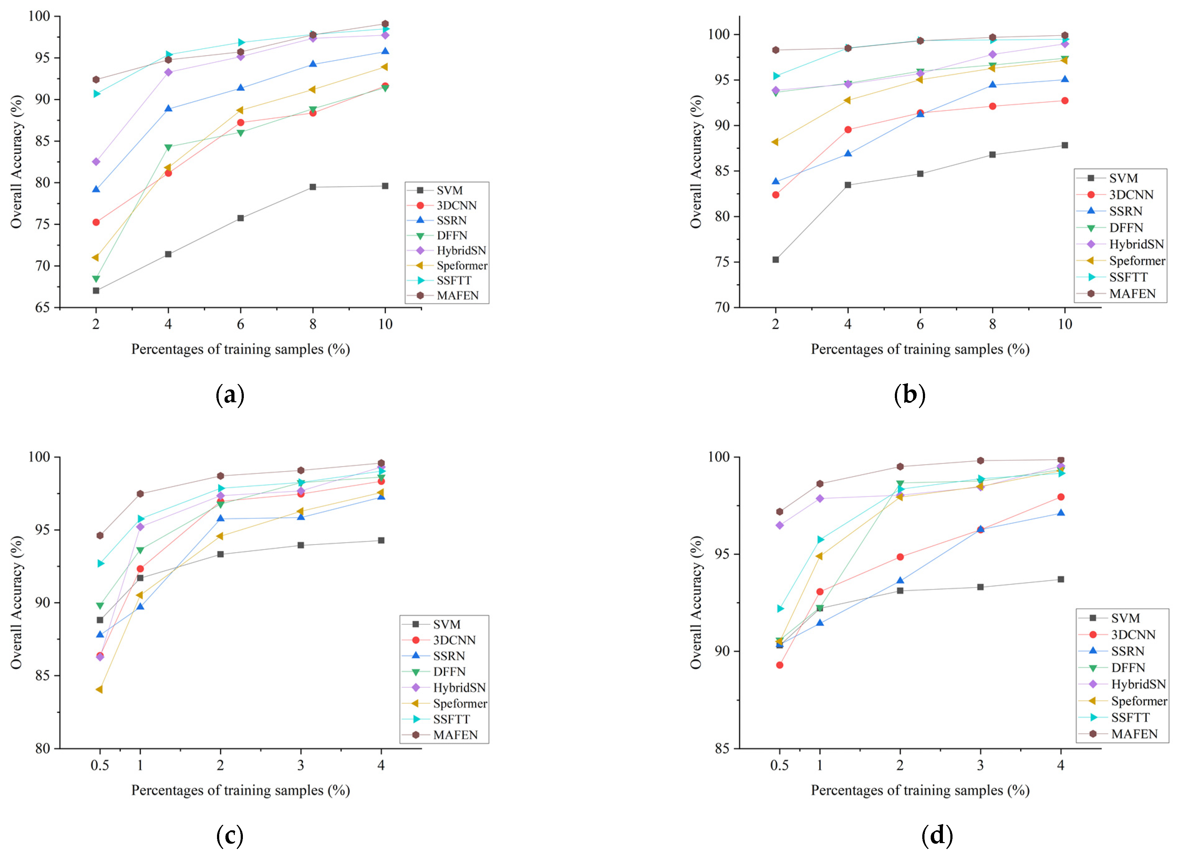
(2) OA of Models with Different Percentages of Training Samples: Figure 12 presents the classification accuracy of various methods with different percentages of training samples. Considering the differences in the number of available samples for each dataset, 2%, 4%, 6%, 8% and 10% of labeled samples were selected as training samples for the Indian Pines and KSC datasets, while 0.5%, 1%, 2%, 3% and 4% of labeled samples were selected as training samples for the Pavia University and Salinas datasets. From Figure 12, it can be seen that the proposed MAFEN method still performed well even with fewer training samples. In addition, as the percentage of training samples increased, the accuracy of various methods also increased. Among them, the accuracy of SSFTT and HybridSN was close to our method, showing better classification performance.

(3) Computational Performance: The results of training and testing time consumed by SSRN, DFFN, HybridSN, Speformer, SSFTT and our proposed MAFEN method are listed in

Table 9. Computational performance comparison of several comparison methods and the proposed method.

Methods	Indian Pines		KSC		Pavia University		Salinas
	Train. (s)	Test. (s)	Train. (s)	Test. (s)	Train. (s)	Test. (s)	Train. (s)	Test. (s)
SSRN	78.90	1.69	115.47	1.90	129.75	9.71	449.59	24.43
DFFN	65.56	1.82	37.79	1.10	83.54	8.26	112.91	11.71
HybridSN	73.85	2.02	40.54	1.02	91.93	9.21	115.28	12.37
Speformer	394.06	23.99	118.99	5.70	58.15	12.07	198.74	52.78
SSFTT	25.18	0.65	26.64	0.76	8.78	1.15	10.79	1.46
MAFEN	66.13	1.93	86.21	2.67	65.59	7.66	88.75	9.76

. It can be seen that there were obvious differences in the training and testing time of several methods on different datasets. Among them, SSFTT was the most computationally efficient, and the training time was much lower than that of the other methods on all datasets. In contrast, the training time of Speformer was longer, especially on the Indian Pines dataset, where the training time was more than four times longer than that of the other models. On the whole, our proposed method performed well with relatively short training time on different datasets.

3.3.3. Ablation Experiment

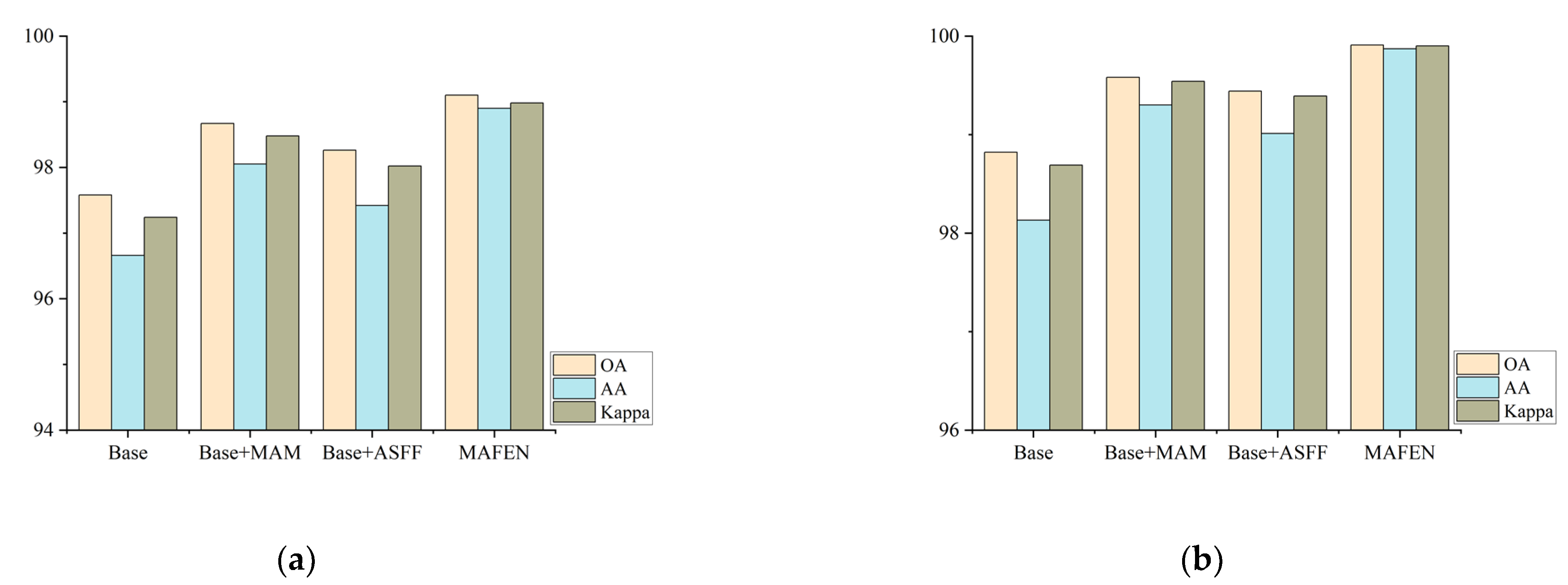
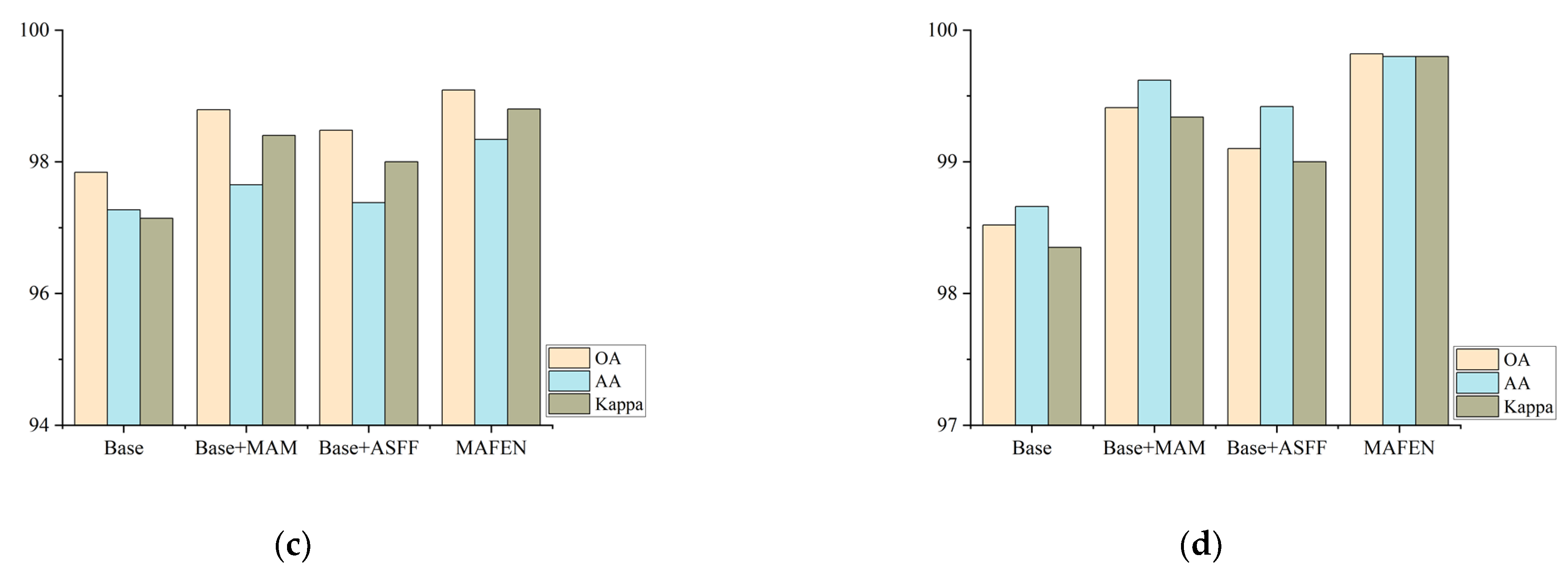
In order to thoroughly validate the effectiveness of each component in the proposed method, the ablation experiment was conducted on the Indian Pines, KSC, Pavia University and Salinas datasets to analyze the impact of the ASFF and MAM components. Four combinations were considered, where the Base network did not contain the MAM and ASFF modules. Three indicators, OA, AA and Kappa, were used to analyze the influence of different components on the whole model, and the experimental results are shown in Figure 13.

The Base network, which did not include the MAM and ASFF modules, had the worst classification performance on the four datasets. When adding the MAM or ASFF module, the classification performance was significantly improved compared with that of the Base network, which verifies the effectiveness of the MAM and ASFF modules. Compared with the network containing the ASFF module, the network containing the MAM module had better improvement performance, showing that the attention mechanism can extract effective spectral–spatial information, which is more helpful to improve the HSI classification performance. The classification performance of the MAFEN network with two modules was better, which reflects the better performance of spectral–spatial features by using both modules simultaneously. In summary, the results of the ablation experiment further prove the effectiveness of the proposed model.

4. Conclusions

The method named Feature Embedding Network with Multiscale Attention (MAFEN) is proposed in this article to improve the classification performance of Hyperspectral Images (HSIs). The MAFEN model first utilizes multiscale attention modules to extract informative features, then embeds deep features into shallow features to enhance the feature representation capability of the network. Finally, adaptive fusion is performed on features at different levels. Experiments were conducted on four commonly used HSI datasets, and comparisons were made with existing methods. The proposed MAFEN method demonstrated superior spectral–spatial feature representation capability, as it effectively utilized spatial details from shallow features and semantic information from deep features, resulting in a significant improvement in classification accuracies on all four datasets compared with those of several other methods. In the future, we will further study new attention-based networks to fully leverage the critical information in HSIs.

References

- Zhang, X.; Liu, L.; Chen, X.; Gao, Y.; Jiang, M. Automatically Monitoring Impervio-us Surfaces Using Spectral Generalization and Time Series Landsat Imagery from1985 to 2020 in the Yangtze River Delta. J. Remote Sens. 2021, 2021, 9873816. [Google Scholar] [CrossRef]
- Yang, X.; Yu, Y. Estimating Soil Salinity Under Various Moisture Conditions: An Experimental Study. IEEE Trans. Geosci. Remote Sens. 2017, 55, 2525–2533. [Google Scholar] [CrossRef]
- Avtar, R.; Sahu, N.; Aggarwal, A.K.; Chakraborty, S.; Kharrazi, A.; Yunus, A.P.; Dou, J.; Kurniawan, T.A. Exploring Renewable Energy Resources Using Remote Sensing and GIS—A Review. Resources 2019, 8, 149. [Google Scholar] [CrossRef]
- Weiss, M.; Jacob, F.; Duveiller, G. Remote Sensing for Agricultural Applications: A Meta-Review. Remote Sens. Environ. 2020, 236, 111402. [Google Scholar] [CrossRef]
- Liang, L.; Di, L.; Zhang, L.; Deng, M.; Qin, Z.; Zhao, S.; Lin, H. Estimation of Crop LAI Using Hyperspectral Vegetation Indices and a Hybrid Inversion Method. Remote Sens. Environ. 2015, 165, 123–134. [Google Scholar] [CrossRef]
- Ye, Q.; Huang, P.; Zhang, Z.; Zheng, Y.; Fu, L.; Yang, W. Multiview Learning WithRobust Double-Sided Twin SVM. IEEE Trans. Cybern. 2022, 52, 12745–12758. [Google Scholar] [CrossRef]
- Haut, J.M.; Paoletti, M.E. Cloud Implementation of Multinomial Logistic Regression for UAV Hyperspectral Images. IEEE J. Miniat. Air Space Syst. 2020, 1, 163–171. [Google Scholar] [CrossRef]
- Li, J.; Bioucas-Dias, J.M.; Plaza, A. Spectral–Spatial Hyperspectral Image Segmentation Using Subspace Multinomial Logistic Regression and Markov Random Fields. IEEE Trans. Geosci. Remote Sens. 2012, 50, 809–823. [Google Scholar] [CrossRef]
- Du, B.; Zhang, L. Random-Selection-Based Anomaly Detector for Hyperspectral Imagery. IEEE Trans. Geosci. Remote Sens. 2011, 49, 1578–1589. [Google Scholar] [CrossRef]
- Du, B.; Zhang, L. Target Detection Based on a Dynamic Subspace. Pattern Recognit. 2014, 47, 344–358. [Google Scholar] [CrossRef]
- Luo, Y.; Cao, X.; Zhang, J.; Cao, X.; Guo, J.; Shen, H.; Wang, T.; Feng, Q. CE-FPN: Enhancing Channel Information for Object Detection. Multimed. Tools Appl. 2021, 81, 30685–30704. [Google Scholar] [CrossRef]
- Obaid, K.B.; Zeebaree, S.R.M.; Ahmed, O.M. Deep Learning Models Based on Image Classification: A Review. Int. J. Sci. Bus. 2020, 4, 75–81. [Google Scholar] [CrossRef]
- Yang, Y.; Hou, Y.-L.; Hou, Z.; Hao, X.; Shen, Y. Image-Level Supervised Instance Segmentation Using Instance-Wise Boundary. In Proceedings of the 2021 IEEE International Conference on Image Processing (ICIP), Anchorage, AK, USA, 19–22 September 2021; pp. 1069–1073. [Google Scholar]
- Zhang, Q.; Yuan, Q.; Li, Z.; Sun, F.; Zhang, L. Combined Deep Prior with Low-Rank Tensor SVD for Thick Cloud Removal in Multitemporal Images. ISPRS J. Photogramm. Remote Sens. 2021, 177, 161–173. [Google Scholar] [CrossRef]
- Liu, J.; Yang, Z.; Liu, Y.; Mu, C. Hyperspectral Remote Sensing Images Deep Feature Extraction Based on Mixed Feature and Convolutional Neural Networks. Remote Sens. 2021, 13, 2599. [Google Scholar] [CrossRef]
- Hong, D.; Gao, L.; Yokoya, N.; Yao, J.; Chanussot, J.; Du, Q.; Zhang, B. More Diverse Means Better: Multimodal Deep Learning Meets Remote-Sensing Imagery Classification. IEEE Trans. Geosci. Remote Sens. 2021, 59, 4340–4354. [Google Scholar] [CrossRef]
- Feng, J.; Zhao, N.; Shang, R.; Zhang, X.; Jiao, L. Self-Supervised Divide-and-Conquer Generative Adversarial Network for Classification of Hyperspectral Images. IEEE Trans. Geosci. Remote Sens. 2022, 60, 1–17. [Google Scholar] [CrossRef]
- Mu, C.; Dong, Z.; Liu, Y. A Two-Branch Convolutional Neural Network Based on Multi-Spectral Entropy Rate Superpixel Segmentation for Hyperspectral Image Classification. Remote Sens. 2022, 14, 1569. [Google Scholar] [CrossRef]
- Cao, X.; Fu, X.; Xu, C.; Meng, D. Deep Spatial-Spectral Global Reasoning Network for Hyperspectral Image Denoising. IEEE Trans. Geosci. Remote Sens. 2022, 60, 1–14. [Google Scholar] [CrossRef]
- Mu, C.; Zeng, Q.; Liu, Y.; Qu, Y. A Two-Branch Network Combined With Robust Principal Component Analysis for Hyperspectral Image Classification. IEEE Geosci. Remote Sens. Lett. 2021, 18, 2147–2151. [Google Scholar] [CrossRef]
- Hu, W.; Huang, Y.; Wei, L.; Zhang, F.; Li, H. Deep Convolutional Neural Networks for Hyperspectral Image Classification. J. Sens. 2015, 2015, 258619. [Google Scholar] [CrossRef]
- Li, Y.; Zhang, H.; Shen, Q. Spectral–Spatial Classification of Hyperspectral Imagery with 3D Convolutional Neural Network. Remote Sens. 2017, 9, 67. [Google Scholar] [CrossRef]
- Zhong, Z.; Li, J.; Luo, Z.; Chapman, M. Spectral–Spatial Residual Network for Hyperspectral Image Classification: A 3-D Deep Learning Framework. IEEE Trans. Geosci. Remote Sens. 2018, 56, 847–858. [Google Scholar] [CrossRef]
- Roy, S.K.; Krishna, G.; Dubey, S.R.; Chaudhuri, B.B. HybridSN: Exploring 3-D–2-D CNN Feature Hierarchy for Hyperspectral Image Classification. IEEE Geosci. Remote Sens. Lett. 2020, 17, 277–281. [Google Scholar] [CrossRef]
- Mu, C.; Liu, Y.; Liu, Y. Hyperspectral Image Spectral–Spatial Classification Method Based on Deep Adaptive Feature Fusion. Remote Sens. 2021, 13, 746. [Google Scholar] [CrossRef]
- Huang, W.; Zhao, Z.; Sun, L.; Ju, M. Dual-Branch Attention-Assisted CNN for Hyperspectral Image Classification. Remote Sens. 2022, 14, 6158. [Google Scholar] [CrossRef]
- Lu, T.; Liu, M.; Fu, W.; Kang, X. Grouped Multi-Attention Network for Hyperspectral Image Spectral-Spatial Classification. IEEE Trans. Geosci. Remote Sens. 2023, 61, 1–12. [Google Scholar] [CrossRef]
- Yu, H.; Zhang, H.; Liu, Y.; Zheng, K.; Xu, Z.; Xiao, C. Dual-Channel Convolution Network with Image-Based Global Learning Framework for Hyperspectral Image Classification. IEEE Geosci. Remote Sens. Lett. 2022, 19, 1–5. [Google Scholar] [CrossRef]
- Zhang, C.; Li, G.; Du, S. Multiscale Dense Networks for Hyperspectral Remote Sensing Image Classification. IEEE Trans. Geosci. Remote Sens. 2019, 57, 9201–9222. [Google Scholar] [CrossRef]
- Song, W.; Li, S.; Fang, L.; Lu, T. Hyperspectral Image Classification with Deep Feature Fusion Network. IEEE Trans. Geosci. Remote Sens. 2018, 56, 3173–3184. [Google Scholar] [CrossRef]
- Zhang, Z.; Liu, D.; Gao, D.; Shi, G. S3Net: Spectral–Spatial–Semantic Network for Hyperspectral Image Classification With the Multiway Attention Mechanism. IEEE Trans. Geosci. Remote Sens. 2022, 60, 1–17. [Google Scholar] [CrossRef]
- Zhang, X.; Sun, G.; Jia, X.; Wu, L.; Zhang, A.; Ren, J.; Fu, H.; Yao, Y. Spectral–Spatial Self-Attention Networks for Hyperspectral Image Classification. IEEE Trans. Geosci. Remote Sens. 2022, 60, 963. [Google Scholar] [CrossRef]
- Mei, S.; Li, X.; Liu, X.; Cai, H.; Du, Q. Hyperspectral Image Classification Using Attention-Based Bidirectional Long Short-Term Memory Network. IEEE Trans. Geosci. Remote Sens. 2022, 60, 1–12. [Google Scholar] [CrossRef]
- Sun, H.; Zheng, X.; Lu, X.; Wu, S. Spectral–Spatial Attention Network for Hyperspectral Image Classification. IEEE Trans. Geosci. Remote Sens. 2020, 58, 3232–3245. [Google Scholar] [CrossRef]
- Ding, L.; Tang, H.; Bruzzone, L. LANet: Local Attention Embedding to Improve the Semantic Segmentation of Remote Sensing Images. IEEE Trans. Geosci. Remote Sens. 2021, 59, 426–435. [Google Scholar] [CrossRef]
- Hong, D.; Han, Z.; Yao, J.; Gao, L.; Zhang, B.; Plaza, A.; Chanussot, J. SpectralFormer: Rethinking Hyperspectral Image Classification with Transformers. IEEE Trans. Geosci. Remote Sens. 2022, 60, 1–15. [Google Scholar] [CrossRef]
- Sun, L.; Zhao, G.; Zheng, Y.; Wu, Z. Spectral–Spatial Feature Tokenization Transformer for Hyperspectral Image Classification. IEEE Trans. Geosci. Remote Sens. 2022, 60, 1–14. [Google Scholar] [CrossRef]
- Lin, T.-Y.; Dollár, P.; Girshick, R.; He, K.; Hariharan, B.; Belongie, S. Feature Pyramid Networks for Object Detection. In Proceedings of the 2017 IEEE Conference on Computer Vision and Pattern Recognition (CVPR), Honolulu, HI, USA, 21–26 July 2017; pp. 936–944. [Google Scholar]
- Yang, Q.; Zhang, T.; Qiu, T.; Xiao, Y.; Jiang, X. Double Feature Pyramid Networks for Classification and Localization on Object Detection. In Proceedings of the 2022 IEEE International Conference on Systems, Man, and Cybernetics (SMC), Prague, Czech Republic, 9–12 October 2022; pp. 1395–1400. [Google Scholar]
- Wenju, L.; Wanghui, C.; Liu, C.; Gan, Z. A Graph Attention Feature Pyramid Network for 3D Object Detection in Point Clouds. In Proceedings of the 2022 7th International Conference on Intelligent Informatics and Biomedical Science (ICIIBMS), Nara, Japan, 24–26 November 2022; Volume 7, pp. 94–98. [Google Scholar]
- Hu, M.; Li, Y.; Fang, L.; Wang, S. A2-FPN: Attention Aggregation Based Feature Pyramid Network for Instance Segmentation. arXiv 2021, arXiv:2105.03186. [Google Scholar]
- Wang, G.; Guo, W.; Wang, Y.; Wang, W. Feature Pyramid Network Based on Double Filter Feature Fusion for Hyperspectral Image Classification. In Proceedings of the 2022 16th IEEE International Conference on Signal Processing (ICSP), Beijing, China, 21–24 October 2022; Volume 1, pp. 240–244. [Google Scholar]
- Fang, L.; Jiang, Y.; Yan, Y.; Yue, J.; Deng, Y. Hyperspectral Image Instance Segmentation Using Spectral–Spatial Feature Pyramid Network. IEEE Trans. Geosci. Remote Sens. 2023, 61, 1–13. [Google Scholar] [CrossRef]
- Ding, C.; Chen, Y.; Li, R.; Wen, D.; Xie, X.; Zhang, L.; Wei, W.; Zhang, Y. Integrating Hybrid Pyramid Feature Fusion and Coordinate Attention for Effective Small Sample Hyperspectral Image Classification. Remote Sens. 2022, 14, 2355. [Google Scholar] [CrossRef]
- Liu, S.; Huang, D.; Wang, Y. Learning Spatial Fusion for Single-Shot Object Detection. arXiv 2019, arXiv:1911.09516. [Google Scholar]
Figure 1.
The overall framework of the MAFEN for hyperspectral image classification. represents the cube corresponding to the HSI input data, , and are three feature maps with different levels of information obtained using 3D-2D convolution, representing low-level features, mid-level features and high-level features, respectively. , and represent the final features of each branch.
Figure 2.
The structure of MAM. (a) The overall framework of MAM. (b) The structure of the spectral–spatial attention module in MAM. Firstly, MAM convolves the features of different levels with three convolutional kernels of different sizes to obtain multi-scale information. Then, cascaded spectral attention and spatial attention are employed to extract effective information from the feature extracted by each convolution kernel.
Figure 3.
Detailed structure diagram of the spectral attention module. The center vector was taken from the input cube .
Figure 4.
A detailed structure diagram of the spatial attention module. is the feature map obtained by global max pooling of along the channel direction.
Figure 5.
The specific structure of ASFF. is the feature obtained by concatenating three different-level features along the channel dimension, , and are the feature fusion weights, represents the weighted features, is the final feature representation.
Figure 6.
False-color images and ground-truth maps. (a) Indian Pines. (b) KSC. (c) Pavia University. (d) Salinas.
Figure 7.
Classification maps of the Indian Pines dataset. (a) SVM (OA = 79.60%); (b) 3DCNN (OA = 91.62%); (c) SSRN (OA = 95.75%); (d) DFFN (OA = 91.43%); (e) HybridSN (OA = 97.73%); (f) Speformer (OA = 93.92%); (g) SSFTT (OA = 98.49%); (h) MAFEN (OA = 99.10%).
Figure 8.
Classification maps of the KSC dataset. (a) SVM (OA = 87.81%); (b) 3DCNN (OA = 92.74%); (c) SSRN (OA = 95.04%); (d) DFFN (OA = 97.39%); (e) HybridSN (OA = 98.98%); (f) Speformer (OA = 97.15%); (g) SSFTT (OA = 99.48%); (h) MAFEN (OA = 99.91%).
Figure 9.
Classification maps of the Pavia University dataset. (a) SVM (OA = 93.94%); (b) 3DCNN (OA = 98.09%); (c) SSRN (OA = 95.76%); (d) DFFN (OA = 98.25%); (e) HybridSN (OA = 97.35%); (f) Speformer (OA = 96.28%); (g) SSFTT (OA = 98.26%); (h) MAFEN (OA = 99.09%).
Figure 10.
Classification maps of the Salinas dataset. (a) SVM (OA = 93.30%); (b) 3DCNN (OA = 96.64%); (c) SSRN (OA = 96.27%); (d) DFFN (OA = 98.77%); (e) HybridSN (OA = 98.46%); (f) Speformer (OA = 98.49%); (g) SSFTT (OA = 98.89%); (h) MAFEN (OA = 99.82%).