Simulation of Seismoelectric Waves Using Time-Domain Finite-Element Method in 2D PSVTM Mode

Abstract

The study of the numerical simulation of seismoelectric effects is very helpful for understanding the theory and mechanism of seismoelectric activities. Quasi-static approximation is widely used in the numerical simulation of seismoelectric fields. However, numerical errors occur when the model domain is not within the near-field area of EM waves or the medium is of high salinity. To solve this problem, we propose a time-domain finite-element algorithm (FETD) based on the full-wave electromagnetic (EM) equation to simulate seismoelectric waves in 2D PSVTM mode. By decomposing the electrokinetic coupling equations into two independent ones, we can solve the seismoelectric waves separately. In our implementation, we focus our attention on the solution of EM waves based on vector–scalar potentials, while using the open-source code SPECFEM2D to explicitly solve Biot’s equations and obtain the relative fluid–solid displacement, which is taken as the source for the complete Maxwell’s equations. In the solution of EM wave fields, we use an unconditionally stable implicit method for time discretization. Computation efficiency can be improved by combining explicit and implicit recursions. After conducting the mathematical formulation, we first validate our method by comparing its results with the analytic solutions for a half-space and a two-layer model, as well as with a quasi-static approximation method. Moreover, we run numerical simulations and wavefield analyses on an elliptical hydrocarbon reservoir, and reveal that the interface responses are promising for the identification of underground interfaces and hydrocarbon reservoir exploration.

1. Introduction

The electrokinetic effect related to the electric double layer in fluid-saturated porous media induces coupling between seismic and electromagnetic (EM) waves, and the conversion between seismic and EM energy induced by this coupling is mutual [1,2,3,4,5,6]. Theoretical simulations and experimental studies have demonstrated that there are three types of seismoelectric conversion under the excitation of mechanical sources [4,7,8,9,10]. The first type is EM waves directly generated by a seismic source [4,11,12], the second type is coseismic EM waves generated by a seismic wave [7,13], and the third type is EM waves generated by a seismic wave at the interface separating two different media (at least one of which is a fluid-saturated porous medium), sometimes called ‘interface responses’ [14,15,16,17]. The seismic EM signal generated in the process of seismoelectric conversion is sensitive to changes in the medium and fluid properties (e.g., the porosity, the permeability, or the salinity), and thus, has promising applications in the detection of deep complex structures and hydrocarbon reservoirs [6,8,9,18,19,20,21,22].

To study the mechanism of the seismoelectric effect and the characteristics of the seismoelectric signal, and to establish theoretical basis for seismoelectric exploration, researchers have developed models to describe the propagation of seismoelectric waves in porous media [1,23,24,25,26,27]. Pride (1994) derived a set of governing equations for the simulation of the seismoelectric effect in saturated porous media using a volume-averaging approach that couples Biot’s equations [28] with Maxwell’s equations via an electrokinetic coupling coefficient characterized by the zeta potential [1]. Revil and Linde (2006) proposed an electrokinetic model coupled with the amount of excess electrical charge in the pore volume that can be used to model unsaturated porous media [23]. Warden et al., (2013) extended Pride’s theory to unsaturated porous media to study the seismoelectric responses of seepage zones under water–air mixture conditions [24]. Zyserman et al., (2017), again, extended Pride’s model by proposing transfer functions connected with water saturation for the electric and magnetic fields [25]. Jougnot (2019, 2021) established a model for frequency-dependent effective excess charge density by mechanically amplifying the electrokinetic coupling in a capillary and simulated the seismoelectric signal [26,27].

Based on the above theoretical models, a large number of analytical and numerical simulation methods have been proposed. The analytical solutions are for full-space models [4,11,29], or horizontally layered models [5,7,16,30,31]. However, the analytical solutions can only deal with simple models, while numerical simulations are needed when irregular interfaces or lateral heterogeneities are involved.

The finite-difference (FD) and finite-element (FE) methods are commonly used in geophysical modeling and are also mainstream techniques in seismoelectric simulations. To model time-domain responses, people generally use indirect and direct methods. Indirect methods calculate EM responses in the frequency domain, and then, transform them into the time domain, while direct methods are carried out directly in the time domain. Among frequency-domain modeling, Zyserman et al., (2010) developed an FE method for solving 2D electroseismic equations that connect diffusing EM waves with seismic waves [32]. Zyserman et al., (2015), again, used the FE method to model the seismoelectric field and studied the EM responses of a partially saturated carbon dioxide model [33]. Gao et al., (2019) applied the frequency-domain FD method (FDFD) to simulate the seismoelectric waves in SHTE mode [17]. Regarding time-domain modeling, Pain et al., (2005) presented a time-domain mixed FE method for the calculation of electric fields generated by the acoustic waves in a borehole [34]. Haines and Pride (2006) developed a time-domain algorithm capable of simulating the seismoelectric conversions in a heterogenous medium [18]. Tohti et al., (2020) calculated the seismoelectric responses for an explosive source based on the time-domain FD (FDTD) algorithm [35], and Tohti et al., (2022) further expanded the seismoelectric coupling equations in 3D orthotropic media to simulate the seismoelectric signal propagating in orthotropic media [36]. Ji et al., (2022) proposed an adaptive time-step high-order FD scheme based on full Maxwell’s equations for a time-varying EM field to simulate the seismoelectric responses in heterogeneous porous saturated media [37]. For the methods that solve the frequency-domain problems, a frequency–time conversion technique needs to be applied to calculate the time-domain responses, and the calculation accuracy is related to the selected frequency range. It is generally necessary to calculate the frequency domain response in a wide frequency range, but this can be computationally expensive and inefficient. If the selected frequency band is not wide enough, inaccuracies may occur. For those methods that work directly in the time domain, a quasi-static approximation is generally performed to separately solve the seismic and EM wave fields, but errors can occur when the model area is not within the near-field area of EM waves [18] or it is in a medium with high salinity [38]. To overcome these disadvantages, we propose, in this paper, an algorithm to simulate seismoelectric responses directly in the time domain based on full-wave EM equations.

Haines and Pride (2006) pointed out that the mechanical disturbances generated by EM fields induced by seismic waves can be ignored in the seismoelectric framework due to weak electroosmotic feedback [18]. Therefore, the decoupling method can be adopted in numerical simulations in the time domain. This means that we can first solve the seismic wave fields from poroelastic dynamic equations, and then, solve the EM fields from Maxwell’s equations. To enhance the calculation efficiency, a combined explicit and implicit scheme is used in the solution. This has the advantage of being able to handle a large velocity difference between EM and seismic waves and to avoid the stability problem with time recursion.

The remainder of this paper is organized as follows. In Section 2, we present the theory and methodology of the FETD algorithm, including the seismoelectric governing equations for the PSVTM mode, and the formulation of the vector–scalar potentials for FE modeling. In Section 3, we verify the effectiveness of our FETD method by comparing its results for a half-space and a two-layer model with the analytic solutions and the quasi-static approximation. In Section 4, we apply the FETD method to an elliptical hydrocarbon reservoir and analyze the characteristics of seismoelectric coupling. We will draw our conclusions based on these numerical models.

2. Methods

2.1. Governing Equations

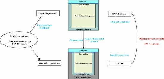
In this paper, we start from Pride’s equations [1] and establish a modeling scheme for the coupled seismic and EM waves in porous media. As we know, in a 2D bounded region, the coupling of a vertically polarized shear wave (SV) and a horizontally polarized magnetic field (TM) with fast longitudinal waves ($P_f$) and slow longitudinal waves ($P_s$) will create PSVTM-mode waves [7,11].

We assume that the SV and TM waves propagate in the x–z plane of a Cartesian coordinate system, with the X-axis positive to the right and the Z-axis positive downward. The solid displacement u, the fluid–solid relative displacement w, and the electric field E, generated by the SV and TM waves have x- and z-components, while the magnetic field H has only a y-component. According to Haines and Pride (2006) [18], the electroosmotic feedback is weak and can be ignored, so that Pride’s equations are decoupled into Biot’s equations and Maxwell’s equations with electrokinetic coupling term. Pride’s equations in the time domain in PSVTM mode can be written as

$$\nabla \cdot \tau =\rho \frac{{\partial }^{2}u}{\partial t^2}+{\rho }_f\frac{{\partial }^{2}w}{\partial t^2},$$

(1)

$$-\nabla P={\rho }_f\frac{{\partial }^{2}u}{\partial t^2}+\frac{{\rho }_f{\alpha }_{\infty }}{\phi }\frac{{\partial }^{2}w}{\partial t^2}+\frac{{\eta }_f}{k}\frac{\partial w}{\partial t},$$

(2)

$$\tau =\left(\left(H-2G\right)\nabla \cdot u+C\nabla \cdot w\right)I+G\left(\nabla u+\nabla u^T\right),$$

(3)

$$P=-C\nabla \cdot u-M\nabla \cdot w,$$

(4)

$$\nabla \times H=\sigma E+\epsilon \frac{\partial E}{\partial t}+L\frac{{\eta }_f}{k}\frac{\partial }{\partial t}w,$$

(5)

$$\nabla \times E=-\mu \frac{\partial H}{\partial t},$$

(6)

where the bulk modulus H, C, M can be expressed by the solid bulk modulus K_s, the frame bulk modulus K_fr, the fluid bulk modulus K_f, and the shear modulus μ_fr, i.e.,

$$\mathsf{\alpha }=1-\frac{K_{fr}}{K_s},$$

(7)

$$M=\frac{K_s{K}_f}{\varphi K_s+\left(\alpha -\varphi \right)K_f},$$

(8)

$$C=\mathsf{\alpha }M,$$

(9)

$$H=K_{fr}+4{\mu }_{fr}/3+{\alpha }^{2}M.$$

(10)

The meanings of the symbols that appeared in Equations (1)–(10) are listed in

Table 1. Symbols and terminologies for porous media.

Symbol	Names
$u_x$, $u_z$, $\mathbf{u}$	Solid displacement
$w_x$, $w_z$, $\mathbf{w}$	Relative fluid–solid displacement $\mathbf{w}=\mathsf{\varphi }\left({\mathit{u}}_s-{\mathit{u}}_f\right)$
$q_x$, $q_z$, $\mathbf{q}$	Relative fluid–solid velocity $\mathbf{q}={\partial }_t\mathbf{w}$
$E_x$, $E_z$, $\mathbf{E}$	Electric field
$H_y$, $\mathbf{H}$	Magnetic field
${\tau }_{xx}$, ${\tau }_{zz}$	Bulk stress
${\tau }_{xz}$	Shear stress
$P$	Pore fluid pressure
$K_s$	Solid bulk modulus
$K_f$	Fluid bulk modulus
$K_{fr}$	Frame bulk modulus
${\mu }_{fr}$	Shear modulus
$\mathsf{\epsilon }$	Bulk electric permittivity $\mathsf{\epsilon }={\epsilon }_0[\left({\epsilon }_f-{\epsilon }_s\right)\varphi /{\alpha }_{\mathrm{\infty }}+{\epsilon }_s]$
${\epsilon }_s$, ${\epsilon }_f$	Relative permittivity of the solid grain and pore fluid
${\epsilon }_0$	Vacuum permittivity
$\rho$	Bulk density $\mathsf{\rho }=\left(1-\varphi \right){\rho }_s+\varphi {\rho }_f$
${\rho }_s$, ${\rho }_f$	Solid grain and pore fluid density
$\varphi$	Porosity
${\alpha }_{\mathrm{\infty }}$	Tortuosity
$\mu$	Bulk magnetic permeability
$\eta$	Pore fluid viscosity
$\mathsf{\sigma }$	Bulk conductivity
$k$	Permeability
$L$	Electrokinetic coupling coefficient
$C_f$	Pore fluid salinity

. Note that although the bulk conductivity $\mathsf{\sigma }$, the permeability k, and the electrokinetic coupling coefficient L are frequency-dependent, we take a low-frequency approximation in the time domain and use only the static conductivity and coupling coefficient in our calculations. Their detailed expressions are given by Haartsen and Pride (1997) [7].

2.2. FETD Scheme

In the following, the seismoelectric forward modeling is divided into two steps, respectively, for the poroelastic waves and EM waves. For poroelastic waves, we use the open-source code SPECFEM2D based on the spectral element (SE) method to solve Equations (1)–(4). Morency and Tromp (2008) gave a detailed introduction to solving poroelastic equations [39]. After the relative fluid–solid displacements and relative fluid–solid velocity fields have been obtained, we take them as the source in the full-wave EM equations and solve Equations (5) and (6) for EM fields.

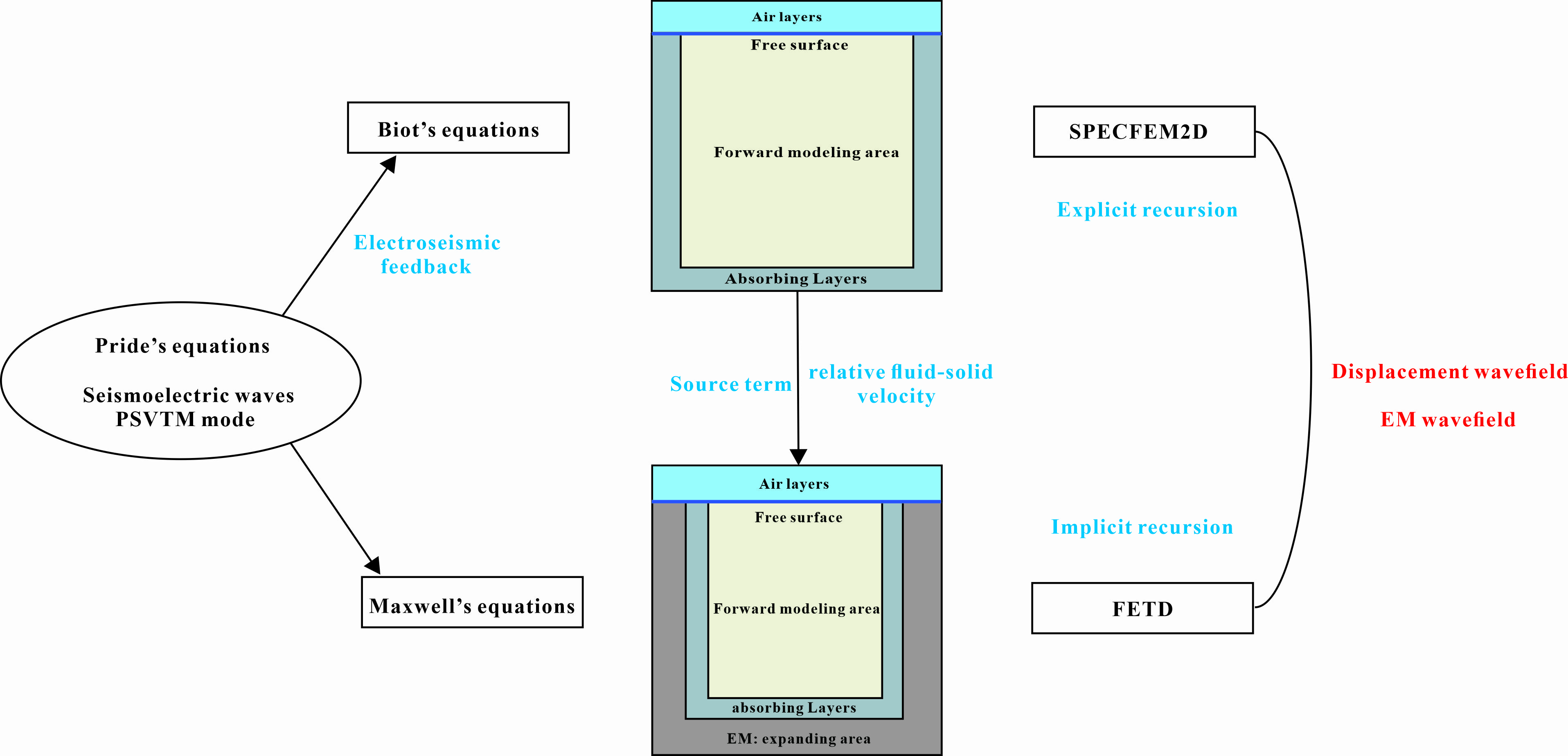
Considering that we take different methods for seismic and EM modeling, we also use different grids for their modeling. Figure 1 shows the distributions and the relationship between the two grids. The area for the seismic simulation is shown on the left, where the yellow grid squares denote the inner modeling area, while the outer grid squares are for the absorbing layer. Since solving full-wave EM equations requires the relative fluid–solid displacements as the source, we take the grids for solving seismic waves as part of the grid for EM simulation. The outermost dark gray part denotes the expanding area for EM simulation. Note that there is a vacuum medium above the blue boundary at the top of the seismic simulation area, and the seismic wave will be totally reflected at the interface, so the displacement field in the vacuum is null. However, for EM fields, the free surface is an interface similar to the underground anomalous interface, and the ‘TM’ waves are not only reflected but also transmitted at the free surface. In actual oil and gas exploration [8,40], the receivers are generally placed near the surface, so it is also necessary to consider the free surface in the simulation of seismoelectric wave fields.

To solve the poroelastic equations using the spectral element method, we take the 4th order of the Gauss–Lobatto–Legendre (GLL) polynomial as the basis function for element interpolations. Meanwhile, to suppress the reflection from artificially truncated boundaries, we use a paraxial approximation of the 1st order of the absorbing boundary conditions proposed by Clayton and Engquist (1977) [41]. To solve the seismoelectric field, we start from the hyperbolic equation obtained from full-wave EM Equations (5) and (6).

The FE simulation for EM problems can be formulated in terms of the coupled vector–scalar potentials or the electric and magnetic fields [42,43]. In this paper, the potential-based nodal finite-element method is used for our simulation. This method does not have stability problems, because the magnetic vector potential and electric scalar potential are essentially continuous at the interfaces when solving the vector and scalar potential A-φ. Additionally, when using the electric and magnetic fields, the electric field equations contain partial derivatives with respect to x and z, which is a second-order linear partial differential equation. However, when solving the vector–scalar potentials, each equation contains only partial derivatives with respect to x or z, and thus, is a 1D wave equation. This transformation makes it easier to apply Dirichlet boundary conditions.

In the following, we present the procedure for the solution of the full-wave EM equations. By introducing a vector magnetic potential A and a scalar electric potential φ, we can write the electric and magnetic fields as

$$H=\frac{1}{\mu }\nabla \times A,$$

(11)

$$E=-\frac{\partial A}{\partial t}-\nabla \phi .$$

(12)

Substituting Equations (11) and (12) into (5) and (6), we obtain the following curl–curl equation for the vector potential:

$$\nabla \times \nabla \times A+\mu \sigma \left(\frac{\partial A}{\partial t}+\nabla \phi \right)+\mu \epsilon \frac{\partial }{\partial t}\left(\frac{\partial A}{\partial t}+\nabla \phi \right)-\mu L\frac{{\eta }_f}{k}q=0.$$

(13)

Due to the existence of the zero space of the curl operator [44], the EM solution will be non-unique if the system is not properly gauged. To ensure the uniqueness of the solution, we apply the Coulomb gauge $\nabla ·\mathbf{A}=0$ to avoid pseudo-solutions. Then, the expansion of the first term in (13) yields

$${\nabla }^{2}A-\mu \sigma \left(\frac{\partial A}{\partial t}+\nabla \phi \right)-\mu \epsilon \frac{\partial }{\partial t}\left(\frac{\partial A}{\partial t}+\nabla \phi \right)+\mu L\frac{{\eta }_f}{k}q=0.$$

(14)

To satisfy the divergence-free condition of the current density $\nabla ·\mathit{J}=0$, we impose an auxiliary equation, i.e.,

$$\nabla \cdot \left(\sigma \left(-\frac{\partial A}{\partial t}-\nabla \phi \right)\right)+\nabla \cdot \left(\epsilon \frac{\partial }{\partial t}\left(-\frac{\partial A}{\partial t}-\nabla \phi \right)\right)+\nabla \cdot \left(L\frac{{\eta }_f}{k}q\right)=0$$

(15)

Since the EM field is very small at locations far from the source, we impose the Dirichlet boundary conditions at the outer boundary, i.e.,

$$A{|}_{\mathsf{\Gamma }}=0, \phi {|}_{\mathsf{\Gamma }}=0.$$

(16)

To solve the potentials A-φ from the above equations, we use the nodal FE method, where the vector potential in the 2D case is decomposed into two scalars in the x- and z-directions. In this way, Equations (14) and (15) can be expanded to

$${\nabla }^2{A}_x-\mu \sigma \left(\frac{\partial A_x}{\partial t}+\frac{\partial \phi }{\partial x}\right)-\mu \epsilon \frac{\partial }{\partial t}\left(\frac{\partial A_x}{\partial t}+\frac{\partial \phi }{\partial x}\right)+\mu L\frac{{\eta }_f}{k}{q}_x=0,$$

(17)

$${\nabla }^2{A}_z-\mu \sigma \left(\frac{\partial A_z}{\partial t}+\frac{\partial \phi }{\partial z}\right)-\mu \epsilon \frac{\partial }{\partial t}\left(\frac{\partial A_z}{\partial t}+\frac{\partial \phi }{\partial z}\right)+\mu L\frac{{\eta }_f}{k}{q}_z=0,$$

(18)

$$\sigma \left(\frac{\partial }{\partial t}\nabla \cdot A+\nabla \cdot \nabla \phi \right)+\epsilon \frac{\partial }{\partial t}\left(\frac{\partial }{\partial t}\nabla \cdot A+\nabla \cdot \nabla \phi \right)-\nabla \cdot \left(L\frac{{\eta }_f}{k}q\right)=0.$$

(19)

Taking the interpolation from the potentials at the nodes and using the Galerkin method to solve (17)–(19), we obtain the following weak form:

$${\left(\nabla \mathit{N},\nabla A_x\right)}_{\Omega }+\mu \sigma {\left(\mathit{N},\frac{\partial A_x}{\partial t}+\frac{\partial \phi }{\partial x}\right)}_{\Omega }+\mu \epsilon \frac{\partial }{\partial t}{\left(\mathit{N},\frac{\partial A_x}{\partial t}+\frac{\partial \phi }{\partial x}\right)}_{\Omega }=\mu L\frac{{\eta }_f}{k}{\left(\mathit{N},q_x\right)}_{\Omega },$$

(20)

$${\left(\nabla \mathit{N},\nabla A_z\right)}_{\Omega }+\mu \sigma {\left(\mathit{N},\frac{\partial A_z}{\partial t}+\frac{\partial \phi }{\partial z}\right)}_{\Omega }+\mu \epsilon \frac{\partial }{\partial t}{\left(\mathit{N},\frac{\partial A_z}{\partial t}+\frac{\partial \phi }{\partial z}\right)}_{\Omega }=\mu L\frac{{\eta }_f}{k}{\left(\mathit{N},q_z\right)}_{\Omega },$$

(21)

$$\frac{\partial }{\partial t}\sigma {\left(\nabla \mathit{N},A\right)}_{\Omega }+\sigma {\left(\nabla \mathit{N},\nabla \phi \right)}_{\Omega }+\epsilon \frac{{\partial }^2}{\partial t^2}{\left(\nabla \mathit{N},A\right)}_{\Omega }+\epsilon \frac{\partial }{\partial t}{\left(\nabla \mathit{N},\nabla \phi \right)}_{\Omega }=L\frac{{\eta }_f}{k}{\left(\nabla \mathit{N},q\right)}_{\Omega },$$

(22)

where $\mathrm{N}={[N_1,N_2,N_3,N_4]}^T$ are the nodal interpolation basis functions, with $N_i=\frac{1}{4}\left(1+{\xi }_i\xi \right)\left(1+{\eta }_i\eta \right)$, $i=\mathrm{1,2},\mathrm{3,4}$; $\mathsf{\Omega }$ denotes the whole model domain, while ${\left(u,v\right)}_{\mathsf{\Omega }}={\int }_{\mathsf{\Omega }}uvd\mathsf{\Omega }$. Expanding (20)–(22), we obtain

$$K_1{A}_x\left(t\right)+K_2\frac{d{A}_x\left(t\right)}{dt}+K_3\phi \left(t\right)+K_4\frac{d^2{A}_x\left(t\right)}{d{t}^2}+K_5\frac{d\phi \left(t\right)}{dt}=K_6{q}_x\left(t\right),$$

(23)

$$K_1{A}_z\left(t\right)+K_2\frac{d{A}_z\left(t\right)}{dt}+K_7\phi \left(t\right)+K_4\frac{d^2{A}_z\left(t\right)}{d{t}^2}+K_8\frac{d\phi \left(t\right)}{dt}=K_6{q}_z\left(t\right),$$

(24)

$$\begin{array}{c}{K}_9\frac{d{A}_x\left(t\right)}{dt}+K_{10}\frac{d{A}_z\left(t\right)}{dt}+K_{11}\phi \left(t\right)+K_{12}\frac{d^2{A}_x\left(t\right)}{d{t}^2}+K_{13}\frac{d^2{A}_z\left(t\right)}{d{t}^2}\\ +K_{14}\frac{d\phi \left(t\right)}{dt}=K_{15}{q}_x\left(t\right)+K_{16}{q}_z\left(t\right)\end{array},$$

(25)

where the matrices K₁–K₁₆ are given in Appendix A.

In Equations (23)–(25), we are still left with the time derivatives. We adopt the unconditionally stable first-order of the implicit backward Euler scheme to perform time discretization, i.e.,

$$\frac{df\left(t\right)}{dt}=\frac{1}{\Delta t}\left(f\left(t+\Delta t\right)-f\left(t\right)\right),$$

(26)

$$\frac{d^{2}f\left(t\right)}{d{t}^2}=\frac{1}{\Delta t^2}\left(f\left(t+2\Delta t\right)+f\left(t\right)-2f\left(t+\Delta t\right)\right).$$

(27)

Since the EM solution process is unconditionally stable, we only need to take care of the stability condition of seismic wave modeling. The time discretization in seismic modeling uses Newmark’s explicit scheme [45]. To ensure the stability of the numerical solution, the time step Δt must satisfy the following CFL condition [46]:

$$\Delta t\le C_{n}min(\Delta x/v),$$

(28)

where C_n denotes the Courant number (smaller than 0.5 in SPECFEM2D). To minimize the numerical dispersion, the spatial step needs to be chosen based on the wavelength of the seismic wave, Δx takes the minimum interval of GLL interpolation points, and the velocity v takes the maximum seismic wave velocity (P wave velocity). By taking, respectively, explicit and implicit time discretization, we only need to comply with the requirement of the time step for seismic wave simulations. The combination of explicit and implicit time recursions can effectively handle the huge velocity difference between EM and seismic waves, and thus, avoid the stability problem with the time recursion.

After the time discretization, the substitution of (26)–(27) into (23)–(25) yields

$$\begin{array}{c}\left(K_1\Delta t^2+K_2\Delta t+K_4\right)A_x^{i+2}\left(t\right)+\left(K_3\Delta t^2+K_5\Delta t\right){\phi }^{i+2}\left(t\right)=\left(K_2\Delta t+2K_4\right)A_x^{i+1}\left(t\right)\\ -K_4{A}_x^i\left(t\right)+K_5\Delta t{\phi }^{i+1}\left(t\right)+K_6\Delta t^2{q}_x^{i+1}\left(t\right)\end{array},$$

(29)

$$\begin{array}{c}\left(K_1\Delta t^2+K_2\Delta t+K_4\right)A_z^{i+2}\left(t\right)+\left(K_7\Delta t^2+K_8\Delta t\right){\phi }^{i+2}\left(t\right)=\left(K_2\Delta t+2K_4\right)A_z^{i+1}\left(t\right)\\ -K_4{A}_z^i\left(t\right)+K_8\Delta t{\phi }^{i+1}\left(t\right)+K_6\Delta t^2{q}_z^{i+1}\left(t\right)\end{array},$$

(30)

$$\begin{array}{c}\left(K_9\Delta t+K_{12}\right)A_x^{i+2}\left(t\right)+\left(K_{10}\Delta t+K_{13}\right)A_z^{i+2}\left(t\right)+\left(K_{11}\Delta t^2+K_{14}\Delta t\right){\phi }^{i+2}\left(t\right)\\ =\left(K_9\Delta t+2K_{12}\right)A_x^{i+1}\left(t\right)+\left(K_{10}\Delta t+2K_{13}\right)A_z^{i+1}\left(t\right)-K_{12}{A}_x^i\left(t\right)-K_{13}{A}_z^i\left(t\right)\\ +K_{14}\Delta t{\phi }^{i+1}\left(t\right)+K_{15}\Delta t^2{q}_x^{i+1}\left(t\right)+K_{16}\Delta t^2{q}_z^{i+1}\left(t\right)\end{array},$$

(31)

Reformulating the above equations in matrix format, we obtain a linear equation system ${\mathbf{K}}^e{\mathbf{u}}^e={\mathbf{b}}^e$ for each element, where the coefficient matrix K^e and the term b^e at the right-hand side are given by

$$K^e=\left(\begin{array}{ccc}{K}_1\Delta t^2+K_2\Delta t+K_4& 0& K_3\Delta t^2+K_5\Delta t\\ 0& K_1\Delta t^2+K_2\Delta t+K_4& K_7\Delta t^2+K_8\Delta t\\ K_9\Delta t+K_{12}& K_{10}\Delta t+K_{13}& K_{11}\Delta t^2+K_{14}\Delta t\end{array}\right),$$

(32)

$$b^e={\left(\begin{array}{c}\left(K_2\Delta t+2K_4\right)A_x^{i+1}\left(t\right)-K_4{A}_x^i\left(t\right)+K_5\Delta t{\phi }^{i+1}\left(t\right)+K_6\Delta t^2{q}_x^{i+1}\left(t\right),\\ \left(K_2\Delta t+2K_4\right)A_z^{i+1}\left(t\right)-K_4{A}_z^i\left(t\right)+K_8\Delta t{\phi }^{i+1}\left(t\right)+K_6\Delta t^2{q}_z^{i+1}\left(t\right),\\ \left(K_9\Delta t+2K_{12}\right)A_x^{i+1}\left(t\right)+\left(K_{10}\Delta t+2K_{13}\right)A_z^{i+1}\left(t\right)-K_{12}{A}_x^i\left(t\right)\\ -K_{13}{A}_z^i\left(t\right)+K_{14}\Delta t{\phi }^{i+1}\left(t\right)+K_{15}\Delta t^2{q}_x^{i+1}\left(t\right)+K_{16}\Delta t^2{q}_z^{i+1}\left(t\right)\end{array}\right)}^{\mathrm{T}}.$$

(33)

Finally, by assembling together the matrix and the right-hand term for each element and applying the Dirichlet boundary condition, we obtain a global linear equation system, i.e.,

$$Ku=b,$$

(34)

where K denotes the coefficient matrix, u denotes the vector and scalar potentials to be solved, and b denotes the source term. We use the MUMPS direct solver [47] to solve the above equation. The MUMPS solver has the advantage that the coefficient matrix K needs only to be decomposed once, and then, the solution at each moment can be obtained via back-substitution of the source term.

After obtaining the potentials, we still need an effective numerical differentiation method to calculate the EM field. In our seismoelectric modeling, we calculate the derivatives of the fields at 4 nodes of each element, and then, obtain the derivatives at the survey points via area-weighted averaging. Finally, we can calculate the EM fields at the survey sites using Equations (11) and (12). For all models, we run our Fortran code on a Dell workstation with 1 CPU of Intel Xeon Gold 6246R @3.40GHz and 512 Gb memory. We will present, in the following, a discussion on time and memory consumption for each specific model.

3. Accuracy Verification

To verify the accuracy of the algorithm presented in this paper, we compare the results from our FETD algorithm with the analytical solutions from Gao and Hu (2010) [4] for different models. Meanwhile, to illustrate the advantages of our algorithm over the quasi-static approximation, we also compare the results from these two methods (see Appendix B).

3.1. A half-Space Model

We first simulate the seismoelectric responses for a half-space model. In Section 3.1 and Section 3.2, we take an explosive point source for our modeling and assume that ${\mathrm{M}}_0=2.54\times {10}^7$ N·m, which is equivalent to 1 kg of explosives [48]. The source function assumes a Ricker wavelet with a central frequency of 30 Hz. The model has a size of 3000 m $\times$ 3000 m. The grid sizes in both directions are 5 m. The source is located 500 m below the free interface. We place a receiver at the upper right corner of the source, 400 m horizontally and 300 m vertically from the source. Here, we take two different salinities for the half-space. The media parameters for the two cases are shown in

Table 2. Parameters of porous media for our modeling.

Symbol	Porous Medium 1	Porous Medium 2	Porous Medium 3	Sandstone 1	Sandstone 2
${\rho }_s (\mathrm{k}\mathrm{g} {\mathrm{m}}^{-3})$	2650	2650	2400	2650	2400
${\rho }_f (\mathrm{k}\mathrm{g} {\mathrm{m}}^{-3})$	1000	1000	1000	1000	980
$\mathsf{\varphi }$	0.1	0.1	0.2	0.2	0.35
${\alpha }_{\infty }$	3	3	3	3	3
$k_s \left(\mathrm{G}\mathrm{p}\mathrm{a}\right)$	12.2	12.2	21.252	12.2	21.252
$k_f \left(\mathrm{G}\mathrm{p}\mathrm{a}\right)$	1.985	1.985	2.25	1.985	2.25
$k_{fr} \left(\mathrm{G}\mathrm{p}\mathrm{a}\right)$	9.6	9.6	7.199	9.6	7.199
${\eta }_f (\mathrm{p}\mathrm{a} \mathrm{s})$	0.001	0.001	0.001	0.001	0.001
${\mu }_{fr} \left(\mathrm{G}\mathrm{p}\mathrm{a}\right)$	5.1	5.1	5.92	5.1	5.92
$v_p (\mathrm{m} {\mathrm{s}}^{-1})$	2628.87	2628.87	2998.17	2695.98	3047.1
$v_s (\mathrm{m} {\mathrm{s}}^{-1})$	1434.92	1434.92	1673.63	1484.23	1765.05
${\epsilon }_s$	4	4	4	4	4
${\epsilon }_f$	80	80	80	80	80
$C_f (\mathrm{m}\mathrm{o}\mathrm{l} {\mathrm{L}}^{-1})$	0.01	5	0.001	0.2	0.001
$\mathrm{k} \left({\mathrm{m}}^2\right)$	$1.0e^{-10}$	$1.0e^{-10}$	$1.0e^{-10}$	$1.0e^{-10}$	$1.0e^{-10}$
$\sigma (\mathrm{S} {\mathrm{m}}^{-1})$	$0.00309$	$1.546$	$0.000618$	$0.124$	$0.00108$
$L (\mathrm{s}\mathrm{C} {\mathrm{k}\mathrm{g}}^{-1})$	$10.388e^{-10}$	$-6.1798e^{-10}$	$33.038e^{-10}$	$4.804e^{-10}$	$57.8067e^{-10}$

as Porous medium 1 and 2, respectively. The conductivity of the air layer is as assumed to be $1e^{-7}$ S/m. Since our FETD method uses implicit time recursion, there will be no stability problem. Here, we use a larger time step (500 time channels) for our modeling and use the direct solver MUMPS to solve the equations system. The degrees of freedom is 1,183,152. This results in memory consumption of 7.4 GB and time consumption of about 1.9 s for each time step.

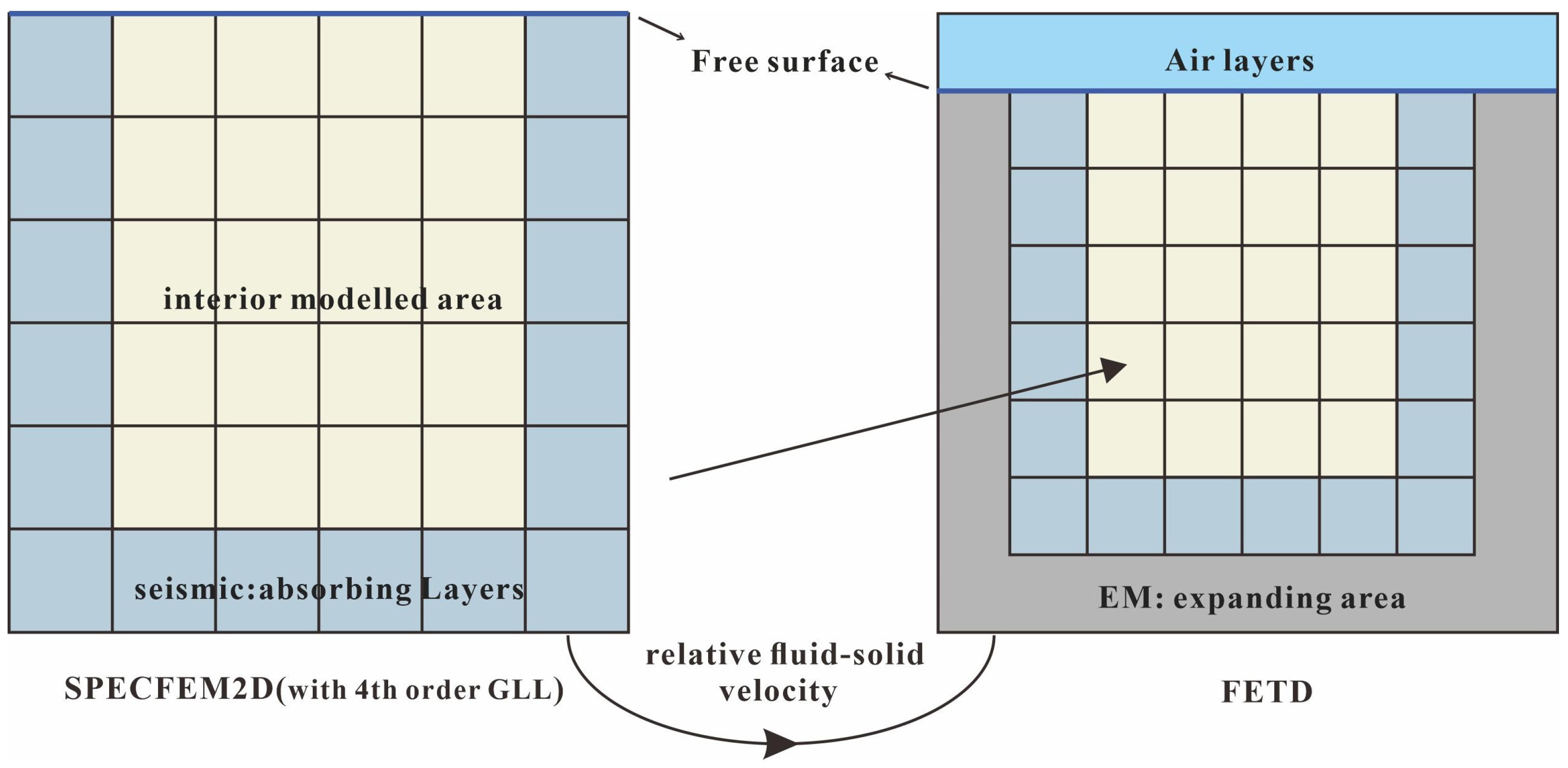
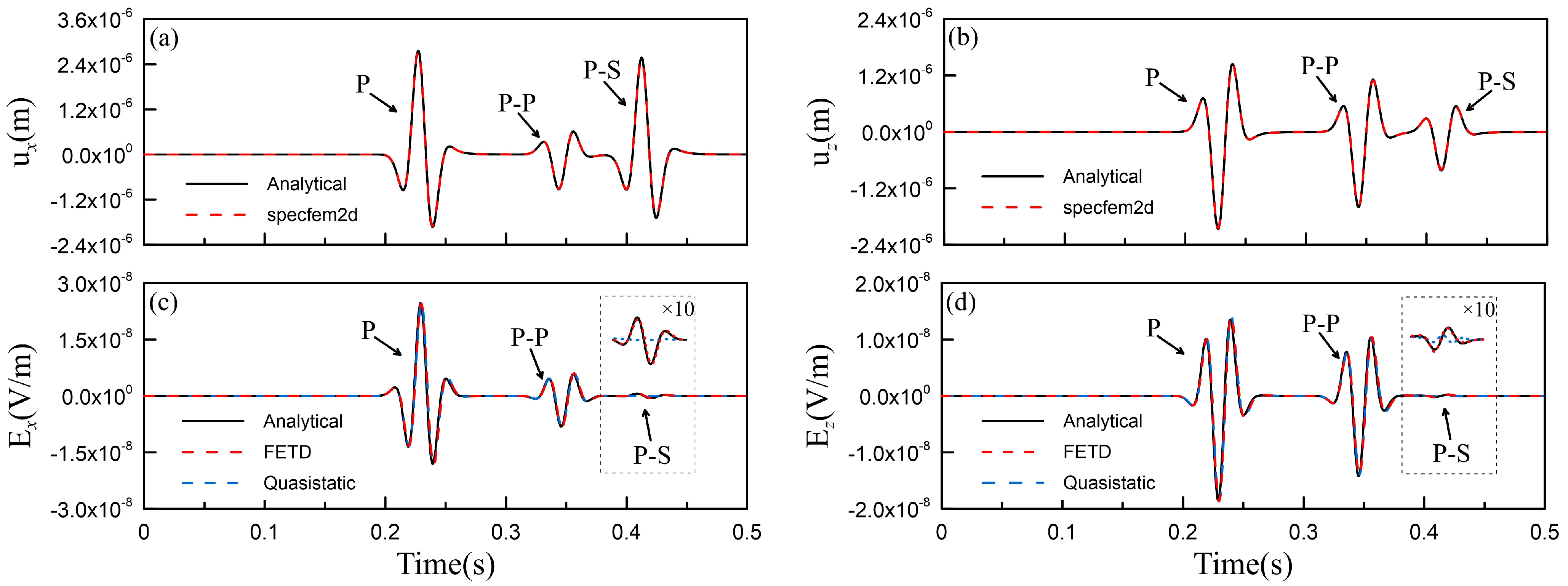
First, for the case of low salinity, we show in Figure 2 the solid displacement and the electric field calculated using the analytical method (black solid lines) and the results of our FETD method (red dashed lines) and quasi-static approximation (blue dashed lines). In Figure 2a,b, the symbol ‘P’ represents the direct P wave with an arrival time of about t = 0.19 s, which is consistent with the theoretical arrival time of 500/2628.87 = 0.19 s. The symbol ‘P-P’ represents the reflected P wave generated by the direct P wave at the free interface, while ‘P-S’ represents the reflected shear wave generated by the direct P wave at the free interface. In Figure 2c,d, ‘P’ represents the coseismic electric field generated by the direct P wave that arrives simultaneously with the direct P wave. ‘P-P’ and ‘P-S’ represent the coseismic electric fields generated by the reflected P wave and S wave at the interface. It is seen from Figure 2 that the results of SPECFEM2D and FETD both match well with the analytical solutions. Since the accompanying electric field generated by the S wave is ignored in the quasi-static approximation [38], we mainly focus on the accompanying electric field of the P-S wave, for which we amplified the amplitude of P-S waves 10 times. Under the condition of low salinity, the electric field induction ability of the S wave is lower than that of the P wave, so the amplitude of the P-S wave coseismic electric field is very small. In this case, the quasi-static approximation also has good agreement with the analytical solution.

Next, we consider the case of high salinity, with its physical properties shown in Table 2 as Porous medium 2. The solid displacement and electric field calculated using the analytical method (black solid lines) and the results of our FETD method (red dashed lines) and quasi-static approximation (blue dashed lines) are shown in Figure 3. Since the mechanical properties of Porous medium 1 and 2 are the same, the solid displacements in Figure 3 are the same as those at low salinity. From Figure 3c,d, one can see that the results of our FETD method match well with the analytical solutions. However, the quasi-static approximation has errors in the accompanying electric field caused by the P-S wave. This is because the ability of the S wave to induce the electric field increases with increasing salinity, and errors will occur when ignoring the accompanying electric field of the S wave [37,38]. In summary, the quasi-static approximation method is effective only in the case of low salinity, while errors may occur in the case of high salinity. This is consistent with Gao et al., (2017) [38]. However, using our FETD method, we can obtain good results in both cases.

3.2. A Two-Layer Model

In the previous section, we found that quasi-static approximation has errors in simulating P-S waves at high salinity. In addition to this, quasi-static approximation also has errors when simulating interface EM waves [38]. In this section, we analyze the interface responses.

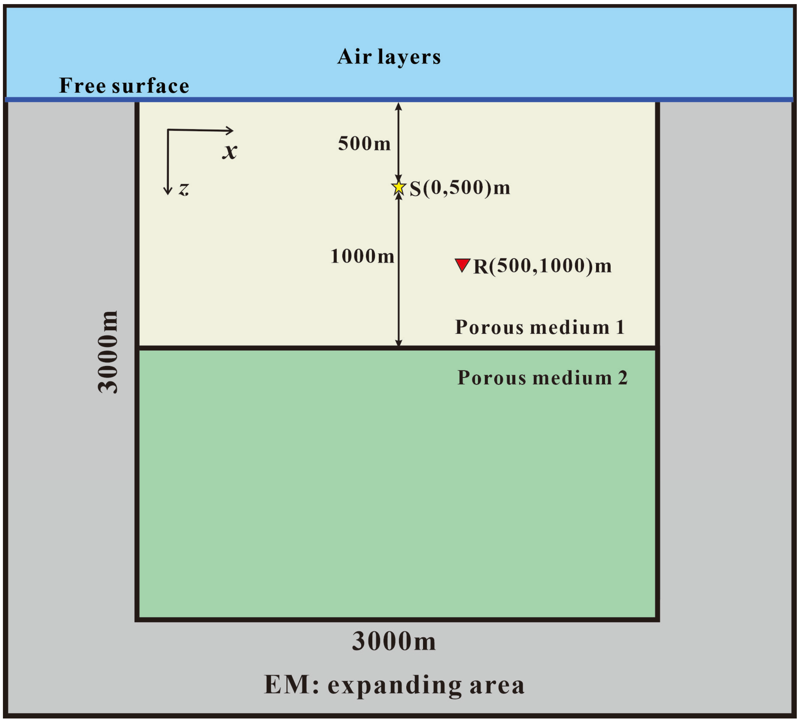
We present a two-layer model and analyze the interface responses at the free surface and the underground interface to further validate our FETD method. The model is shown in Figure 4 with dimensions of 3000 m × 3000 m. The source is located at (0, 500 m), and the layer interface is located at a depth of 1500 m. The grid sizes in both directions are 5 m. The parameters of the upper layer are given in Table 2 as Porous medium 1 (the salinity is set to 1 mol/L, and the corresponding conductivity and electrokinetic coupling coefficient are 0.3092 S/m and −1.889e⁻¹⁰ sC/kg), while those of the lower layer are given in Table 2 as Porous medium 3. We place the receiving point at (500 m, 1000 m), so the distance between the source and the receiver is 707.1 m. Here, we use 1000 time channels for our calculation (one-tenth of the time channels for the simulation of the seismic wave). The degree of freedom is 1,183,152, resulting in memory consumption of 10.2 GB and time consumption of about 8.4 s for each time step.

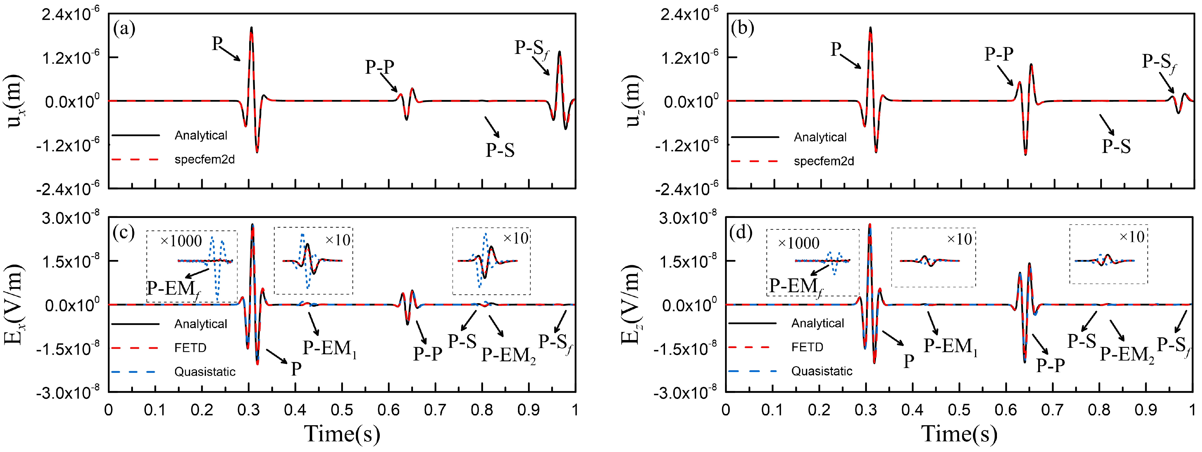
The solid displacement and the electric field calculated using the analytical method are shown in Figure 5 as black solid lines. In Figure 5a,b, the symbol ‘P’ represents the direct longitudinal wave with an arrival time of about t = 0.27 s, which is consistent with the theoretical arrival time of 707.1/2628.87 = 0.27 s. The symbol ‘P-P’ represents the reflected P wave generated by the direct P wave at the free surface and underground interface, while ‘P-S’ and ‘P-S_f’ represent the reflected shear wave generated by the direct P wave at the underground interface and free surface. In Figure 5c,d, ‘P’ represents the coseismic electric field generated by the direct P wave that arrives simultaneously with the direct P wave. ‘P-P’ represents the coseismic electric field generated by the reflected P wave at the interface, while ‘P-S’ and ‘P-S_f’ represent the coseismic electric fields generated by the reflected S wave at the underground interface and free surface, respectively. ‘P-EM_f’ indicates the reflected EM wave generated by the direct P wave at the free surface; its arrival time is t = 0.19 s, which is consistent with the time of the direct P wave traveling from the source to the free surface, 500/2628.87 = 0.19 s. Here, we magnify the interface response 1000 times to make it visible. ‘P-EM₁’ and ‘P-EM₂’ represent the reflected EM wave generated, respectively, by the direct P wave and reflected P wave at the underground interface, and their arrival times are 1000/2628.87 = 0.38 s and (500 × 2 + 1000)/2628.87 = 0.76 s, respectively. Similarly, we amplify the amplitudes 10 times to make the interface response visible. It is worth noting that the arrival times of P-S and P-EM₂ here are basically the same, and what is shown in the interval of 0.75–0.875 s in Figure 5c,d is the superposition of the two waves. From Figure 5c,d, one sees that the results from this paper (red dashed lines) match well with the analytic solutions for both seismic and EM signals. This validates our FETD method for simulating seismoelectric wave fields. However, the quasi-static approximation (blue dashed lines) has large errors in the interface responses. As shown in Figure 5c,d, in the modeling with quasi-static approximation, the reflected EM wave ‘P-EM_f’ generated by the free interface has differences both in amplitude and arrival time. At the same time, we can observe that there are errors in the reflected EM waves generated by the underground interface and the reflected EM waves generated by the P wave reflected by the free surface at the underground interface. Since the upper medium has high salinity (C_f = 1 mol/L), the velocity of the EM waves is 3.115 × 10⁴ m/s at 30 Hz, and the wavelength is about 1038.26 m. The reflection point perpendicular to the interface can be taken as the source of the interface EM waves. The distances from the free interface and the underground interface reflection point to the receiver are 1118.03 and 707.1 m, respectively. In this case, the initial condition of the quasi-static approximation (the distance between the transmitter and receiver needs to be much smaller than the wavelength of EM waves) is not satisfied, so one cannot apply quasi-static approximation [18]. Since the velocity of the EM waves under quasi-static approximation can be taken as the light speed, the time from the interface reflection point to the receiver can be ignored, but in actual fact, it takes a certain time for EM waves to reach the receiver from the free interface and the underground interface reflection point; these times are 1118.03/3.115 × 10⁴ = 0.036 s and 707.1/3.115 × 10⁴ = 0.023 s, respectively. This is also why we see that the interface EM waves calculated using the quasi-static method arrive earlier than those obtained using our FETD algorithm (or the analytical solutions). Meanwhile, since the quasi-static waves only have geometric diffusions but no physical attenuations [38], they have relatively large amplitudes.

The interface responses contain information about the distance between the source and the interface, and thus, are useful for the identification of subsurface structures. This is very helpful in reservoir exploration [14,49,50]. When the model area is not within the near-field area of EM waves or it is in a medium with high salinity [18,38], the quasi-static simulation method will deliver a large interface EM wave that can lead to false anomalies. However, our FETD method has higher accuracy and has advantages in distinguishing subsurface interfaces.

4. Numerical Results

4.1. A Hydrocarbon Reservoir Model with Different Mechanical Properties

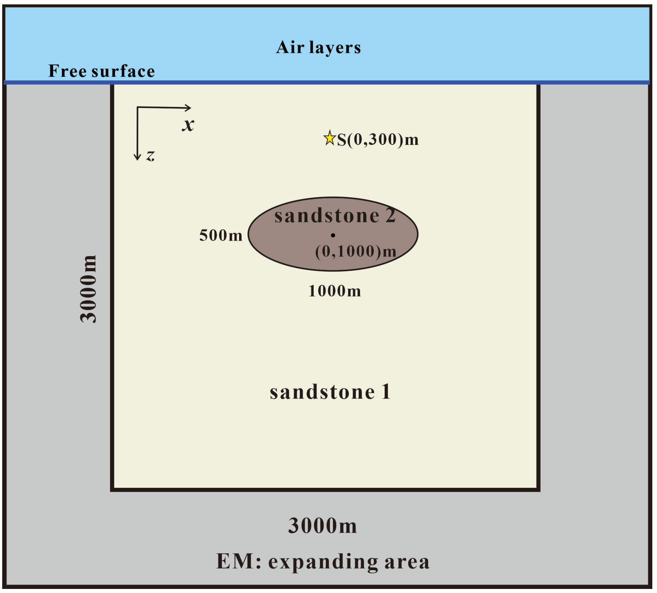
With the theoretical simulation in place, we now apply our FETD method to a reservoir model. In this section, we first assume an elliptical anomalous hydrocarbon reservoir, using similar conductivity in the previous examples [40,51]. The parameters of the reservoir are shown in Table 2 as Sandstone 2, while the parameters for the background sediment are shown in Table 2 as Sandstone 1. As shown in Figure 6, the model domain has a size of 3000 m × 3000 m, and the center of the ellipse is located at (0, 1000 m) with the major axis measuring 1000 m and the minor axis 500 m in length. In this paper, we wish to observe the reflected EM waves at the free interface, so we put the source at (0, 300 m). The source parameters are consistent with those in Section 3. We conduct spatial sampling of 5 m in both the x- and z- directions and place a row of 201 receivers from −500 m to 500 m, and 0.5 m below the free surface. Similarly, we use 1000 time channels for our calculation (one-eighth of the time channels for the seismic simulation). The degree of freedom is 1,183,152, resulting in memory consumption of 10.4 GB and time consumption of about 3.3 s for each time step.

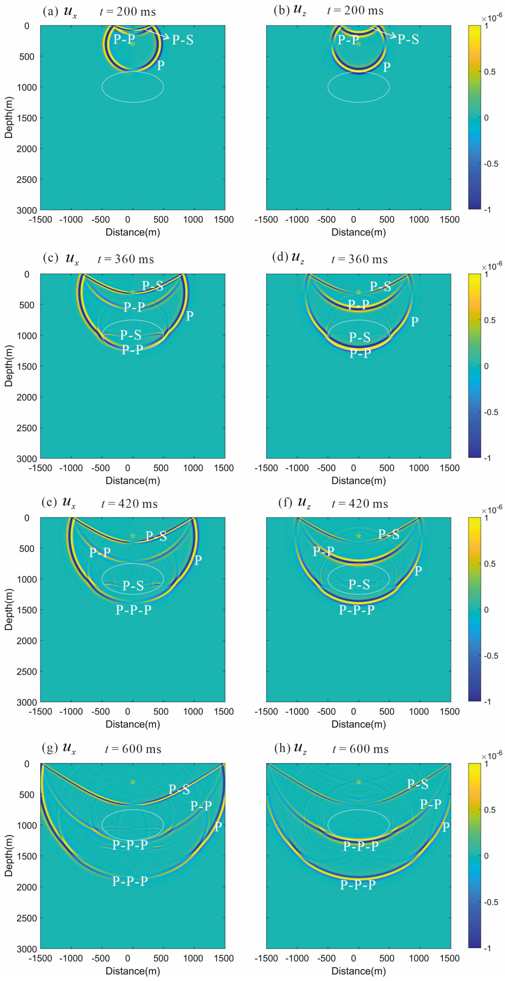
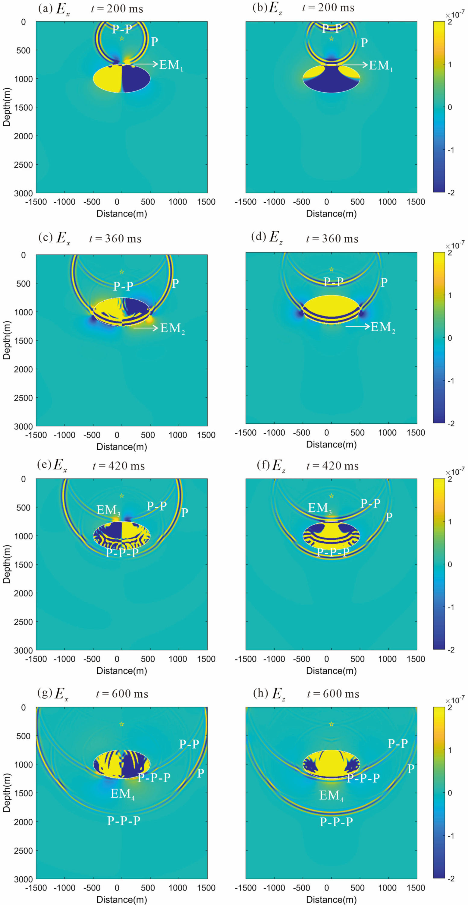
Figure 7 and Figure 8 show wavefield snapshots of the solid displacement and the electric field at four timepoints. From Figure 7a,b, when t = 200 ms, we can see the direct P wave, as well as the reflected P wave and S wave generated by the reflection from the free interface in the displacement snapshots in both the x-and z-directions, while in Figure 8a,b for the corresponding electric field snapshots, the circles show the coseismic electric fields generated by the direct P wave and reflected P wave. The spotlight at the top interface of the elliptical reservoir shows that the direct P wave generates an interfacial EM wave, ‘EM₁’. The EM waves travel much faster than the seismic waves, which means that once the EM waves are generated, they arrive everywhere almost simultaneously. From Figure 7c,d, we can see that at t = 360 ms, the P wave touches the bottom of the reservoir, and another interface EM wave, ‘EM₂’, is generated (Figure 8c,d). From Figure 7e,f, one can see that at t = 420 ms, the direct P wave passes through the bottom interface, the reflected P wave propagates upward, and the transmitted P wave propagates downward. A scattered P wave can also be observed. Meanwhile, the P wave reflected by the free interface propagates downward to the top interface of the elliptical reservoir. Their coseismic electric field can be observed in Figure 8e,f. The spotlight at the top interface of the elliptical reservoir shows that the reflected P wave from the free interface generates an interfacial EM wave, ‘EM₃’. From Figure 7g,h, we can see that at t = 600 ms, and the P wave reflected by the free interface continues to propagate downward, touches the bottom of the reservoir, and generates another interface EM wave, ‘EM₄’ (c.f. Figure 8g,h). Due to the different mechanical properties and salinities of elliptical hydrocarbon reservoir and the sediment, an anomalous boundary can be clearly observed in the electric field snapshots.

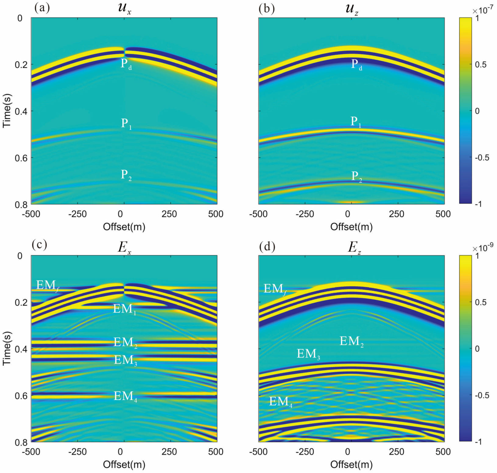
Figure 9 shows the solid displacements and the electric fields for an array of 201 receivers located from −500 m to 500 m, and 0.5 m below the free surface. The symbols ‘P_d’, ‘P₁’, and ‘P₂’ in Figure 9a,b represent, respectively, the direct P wave, the reflected P wave generated by the direct P wave, and the P wave reflected by the free interface reaching the upper boundary of the elliptical reservoir. In Figure 9c,d, the symbols ‘EM_f’, ‘EM₁’, ‘EM₂’, ‘EM₃’, and ‘EM₄’ represent the interfacial EM waves generated when the P waves arrive at different interfaces. The ‘EM_f’ arriving at t = 0.11 s is the EM wave generated by the direct P wave arriving at the free surface. The ‘EM₁’ arriving at t = 0.17 s is the EM wave generated by the direct P wave arriving at the upper interface of the elliptical reservoir. The ‘EM₂’ arriving at t = 0.33 s is the EM wave generated by the transmitted P wave arriving at the lower interface of the elliptical reservoir. The direct P wave passing through the free interface will produce a reflected P wave, and at t = 0.39 s, the ‘EM₃’ wave is generated when the reflected P wave propagates downward to the top interface of the elliptical reservoir. The ‘EM₄’ arriving at t = 0.55 s is the EM wave generated by the transmitted P wave arriving at the lower interface of the elliptical reservoir. The reflected P waves generated by the lower interface will also generate interface EM waves when they propagate upward to the top interface. From the interface EM waves, the positions of the top and bottom interfaces can be inferred. However, to obtain the specific interface shape, additional means are needed, such as changing the positions of the source related to the abnormal interface [51] or adding well-logging information [33].

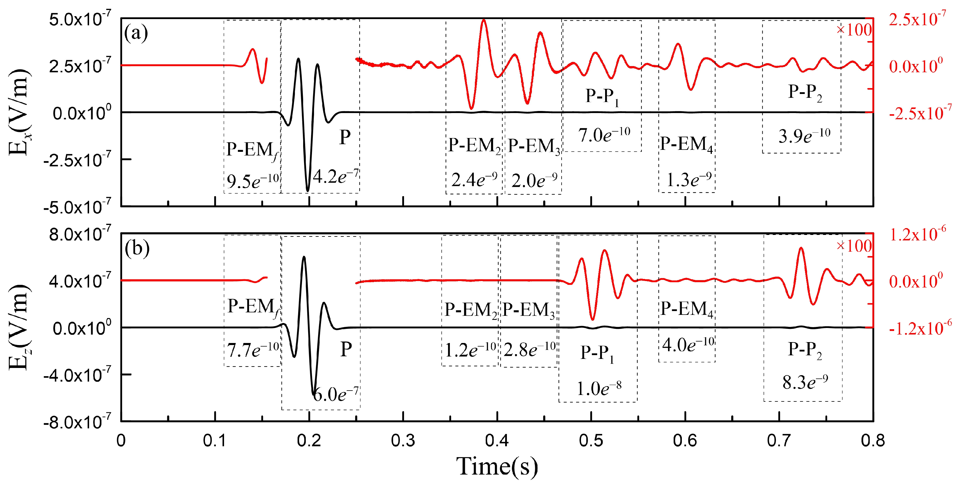
To display the amplitude more clearly, we placed a receiving point at (300 m, 0), and drew a seismogram of the electric field in the x, z-directions, as shown in Figure 10. From Figure 10a, it is seen that the interface electric field in the x-direction is stronger than the accompanying electric field of the reflected P wave, while the amplitude of the accompanying electric field in the z direction is much larger than the interface electric field (c.f. Figure 10b). From the figure, one can also see that the accompanying electric field of the direct P wave is very large, with the magnitude reaching the order of 1.0e⁻⁷ V/m. The accompanying electric field caused by the reflected wave generated by the underground medium has a magnitude in the order of 1.0e⁻⁸ V/m in the z-direction, and the interface EM wave generated at the free interface and underground interface has an order of 1.0e⁻⁹ V/m in the x-direction. It is worth noting that the measurement of the vertical electric field is mostly ignored in practical observations. However, in our simulations, the intensity of the vertical coseismic electric field caused by P waves reflected from the underground interface is 1~2 orders higher than that of the horizontal coseismic electric field. Thus, it is necessary to monitor the vertical electric field in practical seismoelectric observations.

4.2. A Hydrocarbon Reservoir Model with the Same Mechanical Properties

In the previous section, we simulated a hydrocarbon reservoir with different mechanical properties. In actual hydrocarbon exploration, there also exist cases where the mechanical properties of the sediment and reservoir are similar, and they have similar wave impedances [52]. Thus, we consider in this section a case whereby the mechanical properties of the sediment and the reservoir are the same (Sandstone 1 in Table 2), with fluid salinities of 0.2 and 0.001 $\mathrm{m}\mathrm{o}\mathrm{l} {\mathrm{L}}^{-1}$, respectively. Again, we use 1000 time channels in our calculation (one-eighth of the time channels for seismic wave simulation). The degree of freedom is 1,183,152, resulting in memory consumption of 10.5 GB and time consumption of about 3.1 s for each time step.

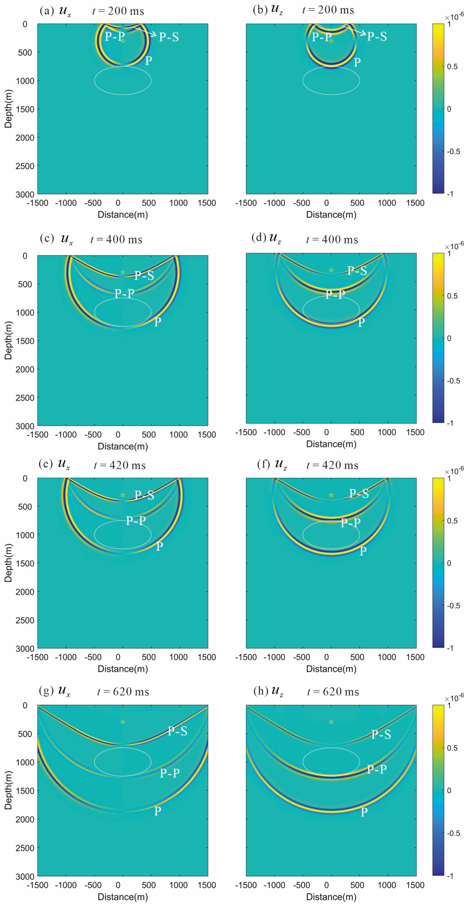
Figure 11 and Figure 12 show snapshots of the solid displacement and the electric field at four timepoints, while Figure 13 shows the solid displacements and the electric fields for an array of 201 receivers located from −500 m to 500 m, and 0.5 m below the free surface. Since the sediment and reservoir have the same mechanical properties, the direct P waves pass through the reservoir interface as if the underground interface does not exist (c.f. Figure 11a–d), and no reflected waves from the underground interface appear in the seismic displacement record (Figure 13a,b). Similarly, the P and S waves reflected from the free surface do not reflect when passing through the reservoir interface (Figure 11e–h).

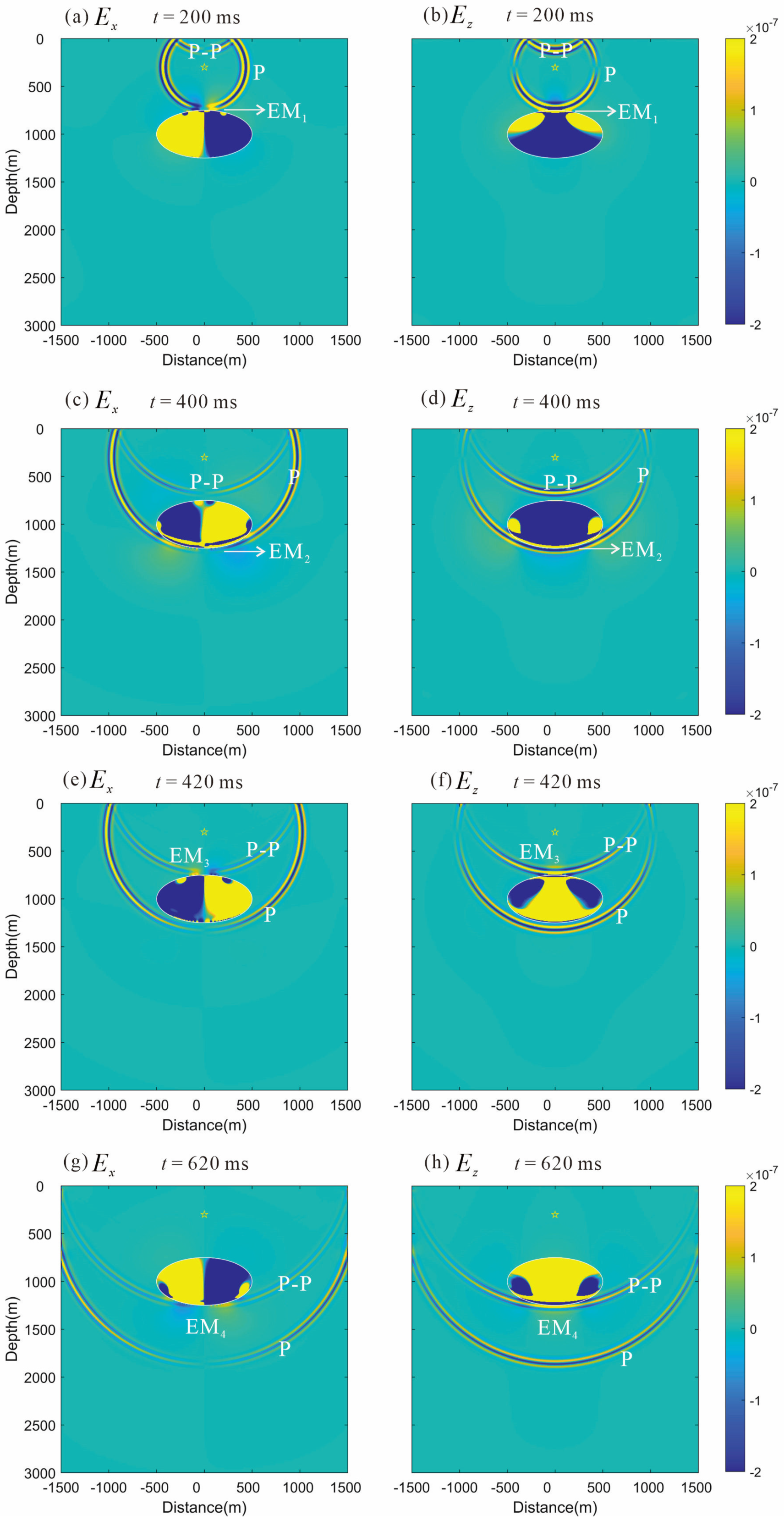
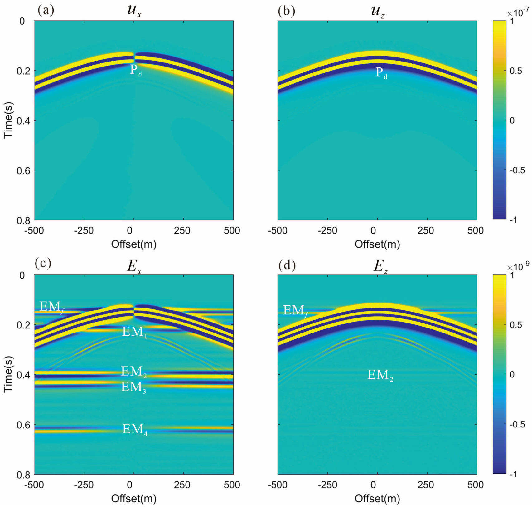
However, since the salinities of the sediment and reservoir are different, the P wave still produces interface responses at the upper and lower interfaces of the reservoir, so we can observe the EM waves in Figure 12a–h and the interface waves in Figure 13c,d. In Figure 13, ‘EM_f’ denotes the EM wave generated by the direct P wave arriving at the free surface, ‘EM₁’ and ‘EM₃’ denote the EM waves generated by the direct P wave and the P wave reflected by the free surface arriving at the upper interface of the reservoir, and ‘EM₂’ and ‘EM₄’ denote the EM waves generated by the direct P wave and the P wave reflected by the free surface arriving at the lower interface of the reservoir. Since the reservoir interface is not reflective, the electric field generated by the reflected wave caused by the bottom interface of the reservoir propagates upward to the upper interface, which appeared in the previous section but no longer exists here. Since there is no mechanical difference, compared to the previous section, we lack coseismic records of the reflected waves, so here, we only focus on interface EM waves. The interface electric field in the vertical direction is much smaller than that in the horizontal direction; only ‘EM_f’ and ‘EM₂’ are marked in Figure 13d. As shown in Figure 13c, the order of magnitude of the interface EM waves generated at the free surface and underground interface in the x-direction are about 1.0e⁻⁹ V/m, which is within the detectable range of current EM monitoring equipment. Therefore, we can determine the position of the top–bottom interface of the reservoir from the interface electric fields in the horizontal direction.

5. Conclusions

Based on vector–scalar potentials, we have successfully developed a FETD method for modeling seismoelectric waves in 2D PSVTM mode. The key to the method is ignoring the electroseismic feedback and decomposition of the Pride macroscopic governing equations in two parts, Biot’s equations and Maxwell’s equations, so that we can first solve Biot’s equations to obtain the displacement and velocity wavefield, and then, take them as the source for solving the full-wave EM equations to obtain the EM field. The numerical results for a half-space and a two-layer model showed that when the model area is not in the near-field area of EM waves or its salinity is high, the traditional quasi-static approximation method has errors when simulating the accompanying electric field of the S wave and the interface responses; however, our FETD solutions still match well with the analytical solutions in seismic and EM fields. At the same time, we use a combination of explicit and implicit recursion that requires fewer time channels to solve the EM equations, and thus, has improved computational efficiency.

Applying our FETD method to the model of an elliptical hydrocarbon reservoir, we found that PSV waves can generate interface EM waves at the free surface and underground interfaces with mechanical or electrical differences, which is consistent with previous research [7,53]. The magnitude of the electric field in the horizontal direction from the interface response can reach the order of 1.0e⁻⁹ V/m, which is detectable by modern instruments [54,55]. This means that we can identify the subsurface structures for reservoir detection from the interface responses. Moreover, although the interface response in the vertical direction is very small and difficult to detect, the accompanying electric field in the vertical direction is 1~2 orders of magnitude larger than those in the horizontal directions, so measurement of the vertical electric field should be carried out in practical exploration. We hope that all of this will help in promoting the seismoelectric application in geophysical explorations. We must point out that in this study, we only consider the conversion from seismic to EM waves in 2D cases. In our future research, we will try to extend our FETD algorithm to the simulation of electroseismic waves and 3D seismoelectric waves.

References

- Pride, S. Governing equations for the coupled electromagnetics and acoustics of porous media. Phys. Rev. B Condens. Matter 1994, 50, 15678–15696. [Google Scholar] [CrossRef]
- Butler, K.E.; Russell, R.D.; Kepic, A.; Maxwell, M. Measurement of the seismoelectric response from a shallow boundary. Geophysics 1996, 61, 1769–1778. [Google Scholar] [CrossRef]
- Zhu, Z.; Haartsen, M.W.; Toksöz, M.N. Experimental studies of seismoelectric conversions in fluid-saturated porous media. J. Geophys. Res. Solid Earth 2000, 105, 28055–28064. [Google Scholar] [CrossRef]
- Gao, Y.; Hu, H. Seismoelectromagnetic waves radiated by a double couple source in a saturated porous medium. Geophys. J. Int. 2010, 181, 873–896. [Google Scholar] [CrossRef]
- Ren, H.; Huang, Q.; Chen, X. A new numerical technique for simulating the coupled seismic and electromagnetic waves in layered porous media. Earthq. Sci. 2010, 23, 167–176. [Google Scholar] [CrossRef]
- Grobbe, N.; Slob, E. Seismo-electromagnetic thin-bed responses: Natural signal enhancements? J. Geophys. Res. Solid Earth 2016, 121, 2460–2479. [Google Scholar] [CrossRef]
- Haartsen, M.W.; Pride, S.R. Electroseismic waves from point sources in layered media. J. Geophys. Res. Atmos. 1997, 102, 24745–24769. [Google Scholar] [CrossRef]
- Thompson, A.H.; Gist, G.A. Geophysical applications of electrokinetic conversion. Lead. Edge 1993, 12, 1169–1173. [Google Scholar] [CrossRef]
- Peng, R.; Di, B.; Glover, P.W.J.; Wei1, J.; Lorinczi, P.; Ding, P.; Liu, Z.; Zhang, Y.; Wu, M. The effect of rock permeability and porosity on seismoelectric conversion: Experiment and analytical modelling. Geophys. J. Int. 2019, 219, 328–345. [Google Scholar] [CrossRef]
- Wang, J.; Zhu, Z.; Gao, Y.; Morgan, F.D.; Hu, H. Measurements of the seismoelectric responses in a synthetic porous rock. Geophys. J. Int. 2020, 222, 436–448. [Google Scholar] [CrossRef]
- Pride, S.R.; Haartsen, M.W. Electroseismic wave properties. J. Acoust. Soc. Am. 1996, 100, 1301–1315. [Google Scholar] [CrossRef]
- Haines, S.S.; Pride, S.R.; Klemperer, S.; Biondi, B. Seismoelectric imaging of shallow targets. Geophysics 2007, 72, G9–G20. [Google Scholar] [CrossRef]
- Bordes, C.; Jouniaux, L.; Garambois, S.; Dietrich, M.; Pozzi, J.-P.; Gaffet, S. Evidence of the theoretically predicted seismo-magnetic conversion. Geophys. J. Int. 2008, 174, 489–504. [Google Scholar] [CrossRef]
- Schakel, M.D.; Smeulders, D.M.J.; Slob, E.; Heller, H.K.J. Seismoelectric interface response: Experimental results and forward model. Geophysics 2011, 76, N29–N36. [Google Scholar] [CrossRef]
- Ren, H.; Huang, Q.; Chen, X. Numerical simulation of seismo-electromagnetic fields associated with a fault in a porous medium. Geophys. J. Int. 2016, 206, 205–220. [Google Scholar] [CrossRef]
- Gao, Y.; Wang, M.; Hu, H.; Chen, X. Seismoelectric responses to an explosive source in a fluid above a fluid-saturated porous medium. J. Geophys. Res. Solid Earth 2017, 122, 7190–7218. [Google Scholar] [CrossRef]
- Gao, Y.; Wang, N.; Yao, C.; Guan, W.; Hu, H.; Wen, J.; Zhang, W.; Tong, P.; Yang, Q. Simulation of seismoelectric waves using finite-difference frequency-domain method: 2D SHTE mode. Geophys. J. Int. 2019, 216, 418–438. [Google Scholar] [CrossRef]
- Haines, S.S.; Pride, S.R. Seismoelectric numerical modeling on a grid. Geophysics 2006, 71, N57–N65. [Google Scholar] [CrossRef]
- Smeulders, D.D.; Grobbe, N.; Heller, H.; Schakel, M. Seismoelectric Conversion for the Detection of Porous Medium Interfaces between Wetting and Nonwetting Fluids. Vadose Zone J. 2014, 13, 1–7. [Google Scholar] [CrossRef]
- Ma, X.; Liu, Y.; Yin, C.; Zhang, B.; Ren, X. Estimation of fluid salinity using coseismic electric signal generated by an earthquake. Geophys. J. Int. 2022, 233, 127–144. [Google Scholar] [CrossRef]
- Peng, R.; Huang, X.; Liu, Z.; Li, H.; Di, B.; Wei, J. Numerical investigation on seismoelectric wave fields in porous media: Porosity and permeability. J. Geophys. Eng. 2023, 20, 1–11. [Google Scholar] [CrossRef]
- Grobbe, N.; Revil, A.; Zhu, Z.; Slob, E. Seismoelectric Exploration: Theory, Experiments, and Applications; John Wiley & Sons: Hoboken, NJ, USA, 2020; Volume 252. [Google Scholar]
- Revil, A.; Linde, N. Chemico-electromechanical coupling in microporous media. J. Colloid Interface Sci. 2006, 302, 682–694. [Google Scholar] [CrossRef] [PubMed]
- Warden, S.; Garambois, S.; Jouniaux, L.; Brito, D.; Sailhac, P.; Bordes, C. Seismoelectric wave propagation numerical modelling in partially saturated materials. Geophys. J. Int. 2013, 194, 1498–1513. [Google Scholar] [CrossRef]
- Zyserman, F.; Monachesi, L.; Jouniaux, L. Dependence of shear wave seismoelectrics on soil textures: A numerical study in the vadose zone. Geophys. J. Int. 2016, 208, 918–935. [Google Scholar] [CrossRef]
- Jougnot, D. New approach to up-scale the frequency-dependent effective excess charge density for seismoelectric modeling. In Proceedings of the SEG Technical Program Expanded Abstracts; Society of Exploration Geophysicists: Houston, TX, USA, 2019; pp. 3608–3612. [Google Scholar] [CrossRef]
- Jougnot, D.; Solazzi, S.G. Predicting the frequency-dependent effective excess charge density: A new upscaling approach for seismoelectric modeling. Geophysics 2021, 86, WB19–WB28. [Google Scholar] [CrossRef]
- Biot, M.A. Theory of Propagation of Elastic Waves in a Fluid-Saturated Porous Solid. I. Low-Frequency Range. J. Acoust. Soc. Am. 1956, 28, 168–178. [Google Scholar] [CrossRef]
- Slob, E.; Mulder, M. Seismoelectromagnetic homogeneous space Green’s functions. Geophysics 2016, 81, F27–F40. [Google Scholar] [CrossRef]
- Hu, H.; Gao, Y. Electromagnetic field generated by a finite fault due to electrokinetic effect. J. Geophys. Res. 2011, 116, 7958. [Google Scholar] [CrossRef]
- Cheng, Q.; Gao, Y.; Zhou, G.; Chen, C.-H.; Wang, D.; Yao, C. Seismoelectric waves generated by a point source in horizontally stratified vertical transversely isotropic porous media. Geophysics 2023, 88, C53–C78. [Google Scholar] [CrossRef]
- Zyserman, F.I.; Gauzellino, P.M.; Santos, J.E. Finite element modeling of SHTE and PSVTM electroseismics. J. Appl. Geophys. 2010, 72, 79–91. [Google Scholar] [CrossRef]
- Zyserman, F.I.; Jouniaux, L.; Warden, S.; Garambois, S. Borehole seismoelectric logging using a shear-wave source: Possible application to CO2 disposal? Int. J. Greenh. Gas Control 2015, 33, 89–102. [Google Scholar] [CrossRef]
- Pain, C.C.; Saunders, J.H.; Worthington, M.H.; Singer, J.M.; Stuart-Bruges, W.; Mason, G.; Goddard, A. A mixed finite-element method for solving the poroelastic Biot equations with electrokinetic coupling. Geophys. J. Int. 2005, 160, 592–608. [Google Scholar] [CrossRef]
- Tohti, M.; Wang, Y.; Slob, E.; Zheng, Y.; Chang, X.; Yao, Y. Seismoelectric numerical simulation in 2D vertical transverse isotropic poroelastic medium. Geophys. Prospect. 2020, 68, 1927–1943. [Google Scholar] [CrossRef]
- Tohti, M.; Wang, Y.; Xiao, W.; Zhou, K. Numerical simulation of seismoelectric wavefields in 3D orthorhombic poroelastic medium. Chin. J. Geophys. 2022, 65, 4471–4484. [Google Scholar] [CrossRef]
- Ji, Y.; Han, L.; Huang, X.; Zhao, X.; Jensen, K.; Yu, Y. A high-order finite-difference scheme for time-domain modeling of time-varying seismoelectric waves. Geophysics 2022, 87, T135–T146. [Google Scholar] [CrossRef]
- Gao, Y.; Huang, F.; Hu, H. Comparison of full and quasi-static seismoelectric analytically based modeling. J. Geophys. Res. Solid Earth 2017, 122, 8066–8106. [Google Scholar] [CrossRef]
- Morency, C.; Tromp, J. Spectral-element simulations of wave propagation in porous media. Geophys. J. Int. 2008, 175, 301–345. [Google Scholar] [CrossRef]
- Thompson, A.H.; Hornbostel, S.; Burns, J.; Murray, T.; Raschke, R.; Wride, J.; McCammon, P.; Sumner, J.; Haake, G.; Bixby, M.; et al. Field tests of electroseismic hydrocarbon detection. Geophysics 2007, 72, N1–N9. [Google Scholar] [CrossRef]
- Clayton, R.; Engquist, B. Absorbing boundary conditions for acoustic and elastic wave equations. Bull. Seism. Soc. Am. 1977, 67, 1529–1540. [Google Scholar] [CrossRef]
- Barton, M.L.; Cendes, Z.J. New vector finite elements for three-dimensional magnetic field computation. J. Appl. Phys. 1987, 61, 3919–3921. [Google Scholar] [CrossRef]
- Biro, O.; Preis, K. On the use of the magnetic vector potential in the finite-element analysis of three-dimensional eddy currents. IEEE Trans. Magn. 1989, 25, 3145–3159. [Google Scholar] [CrossRef]
- Allaire, G.S.M.K. Numerical Linear Algebra; Springer: New York, NY, USA, 2008. [Google Scholar]
- Hughes, T.J.R. The Finite Element Method: Linear Static and Dynamic Finite Element Analysis; Courier Corporation: Englewood Cliffs, NJ, USA, 1987. [Google Scholar]
- De Basabe, J.D.; Sen, M.K. Stability of the high-order finite elements for acoustic or elastic wave propagation with high-order time stepping. Geophys. J. Int. 2010, 181, 577–590. [Google Scholar] [CrossRef]
- Amestoy, P.R.; Guermouche, A.; L’excellent, J.-Y.; Pralet, S. Hybrid scheduling for the parallel solution of linear systems. Parallel Comput. 2006, 32, 136–156. [Google Scholar] [CrossRef]
- Garambois, S.; Dietrich, M. Full waveform numerical simulations of seismoelectromagnetic wave conversions in fluid-saturated stratified porous media. J. Geophys. Res. Solid Earth 2002, 107, ESE 5-1–ESE 5-18. [Google Scholar] [CrossRef]
- Dzieran, L.; Thorwart, M.; Rabbel, W.; Ritter, O. Quantifying interface responses with seismoelectric spectral ratios. Geophys. J. Int. 2019, 217, 108–121. [Google Scholar] [CrossRef]
- Monachesi, L.B.; Zyserman, F.I.; Jouniaux, L. An analytical solution to assess the SH seismoelectric response of the vadose zone. Geophys. J. Int. 2018, 213, 1999–2019. [Google Scholar] [CrossRef]
- Wang, D.; Gao, Y.; Tong, P.; Wang, J.; Yao, C.; Wang, B. Electroseismic and seismoelectric responses at irregular interfaces: Possible application to reservoir exploration. J. Pet. Sci. Eng. 2021, 202, 108513. [Google Scholar] [CrossRef]
- Sheriff, R.E.; Geldart, L.P. Exploration Seismology; Cambridge University Press: Cambridge, UK, 1995. [Google Scholar]
- Garambois, S.; Dietrich, M. Seismoelectric wave conversions in porous media: Field measurements and transfer function analysis. Geophysics 2001, 66, 1417–1430. [Google Scholar] [CrossRef]
- Crespy, A.; Revil, A.; Linde, N.; Byrdina, S.; Jardani, A.; Bolève, A.; Henry, P. Detection and localization of hydromechanical disturbances in a sandbox using the self-potential method. J. Geophys. Res. Atmos. 2008, 113. [Google Scholar] [CrossRef]
- Jardani, A.; Revil, A.; Slob, E.; Söllner, W. Stochastic joint inversion of 2D seismic and seismoelectric signals in linear poroelastic materials: A numerical investigation. Geophysics 2010, 75, N19–N31. [Google Scholar] [CrossRef]
Figure 1.
Mapping relationship between seismic and EM grids. The grids on the left are for seismic modeling with SPECFEM2D, the yellow grids are for the inner simulation region, and the outer light gray grids are for the absorbing layer, with the top blue boundary being the free surface. The grids on the right are for EM modeling with FETD, the inner region is the same as the seismic grids, and the outermost dark gray region is the expanding area, with the air layer above the top blue interface. The two grids are connected by a relative fluid–solid velocity field.
Figure 2.
Comparison of FETD results (red dashed lines) and quasi-static approximation (blue dashed lines) with analytical solutions (black solid lines) for a half-space model at low salinity. To make the reflected S wave response clearer, the signal of 0.39–0.45s is amplified 10 times. (a) Solid displacement ; (b) solid displacement ; (c) electric field ; (d) electric field .
Figure 3.
Comparison of FETD results (red dashed lines) and quasi-static approximation (blue dashed lines) with analytical solutions (black solid lines) for a half-space model at high salinity. To make the reflected S wave response clearer, the signal of 0.39–0.45s is amplified 10 times. (a) Solid displacement ; (b) solid displacement ; (c) electric field ; (d) electric field .
Figure 4.
A two-layer model for FETD modeling. The star denotes the source, while the triangle denotes the receiver. The inner yellow and green areas denote the forward modeling area, while the horizontal black line denotes the interface between two porous media. The gray area denotes the expanding area for absorbing EM waves and the top blue boundary denotes the free surface, with the air layers in the area above.
Figure 5.
Comparison of FETD results (red dashed lines) and quasi-static approximation (blue dashed lines) with analytical solutions (black solid lines) for the two-layer model in Figure 4. The symbol ‘P’ represents the P wave generated directly by the source, and ‘P-P’ and ‘P-S’ represent the reflected P and S waves, respectively. ‘P-EMf’ represents the EM waves generated by the direct P wave at the free surface, and ‘P-EM1’ and ‘P-EM2’ represent the EM waves generated by the direct P wave and reflected P wave at the underground interface, respectively. To make the interface response clearer, the signal at time ranges of 0.15–0.265 s, 0.375–0.5 s, and 0.75–0.875 s is amplified. (a) Solid displacement ; (b) solid displacement ; (c) electric field ; (d) electric field .
Figure 6.
An elliptical hydrocarbon reservoir model for FETD modeling. The star denotes the source, the yellow area denotes the forward modeling domain, while the brown ellipse denotes the anomalous body. The gray area denotes the expanding area for absorbing EM waves, and the top blue boundary is the free surface, with the air layers above.
Figure 7.
Snapshots of the solid displacement , at four moments (t = 200, 360, 420, and 600 ms). The stars denote the sources. The symbol ‘P’ represents the direct P wave, ‘P-P’ represents the reflected and transmitted P waves generated by the direct P wave at the free surface and underground interface, ‘P-S’ represents the reflected and transmitted shear waves generated by the direct P wave at the free surface and underground interface, and ‘P-P-P’ represents the transmitted P wave generated by the reflected and transmitted P waves at the lower interface of the elliptical reservoir.
Figure 8.
Snapshots of the electric field , at four moments (t = 200, 360, 420, and 600 ms). The stars denote the sources. The symbols ‘P’, ‘P-P’, and ‘P-P-P’ represent the coseismic electric fields generated by the corresponding P wave. The symbols ‘EM1’ and ‘EM3’ represent the EM waves generated by the direct P wave and reflected P wave arriving at the upper interface of the elliptical reservoir. The symbols ‘EM2’ and ‘EM4’ represent the EM waves generated by the transmitted P wave arriving at the lower interface of the elliptical reservoir.
Figure 9.
(a,b) show seismograms of the solid displacement , while (c,d) show the electric field , at 201 receiver locations from −500 m to 500 m, and 0.5 m below the free surface.
Figure 10.
(a,b) show seismograms of the electric field , at the surface receiver (300 m, 0). The red line in the figure shows the signal amplified 100 times. Each corresponding wave is marked with a dotted-line box, and the numbers in the box show the maximum amplitude of the corresponding wave.
Figure 11.
Snapshots of the solid displacement , at four moments (t = 200, 400, 420, and 620 ms). The stars denote the sources. The symbol ‘P’ represents the direct P wave, ‘P-P’ represents the reflected P wave generated by the direct P wave at the free surface, and ‘P-S’ represents the reflected shear wave generated by the direct P wave at the free surface.
Figure 12.
Snapshots of the electric field , at four moments (t = 200, 400, 420, and 620 ms). The stars denote the sources. The symbols ‘P’ and ‘P-P’ represent the coseismic electric fields generated by the direct and reflected P waves. The symbols ‘EM1’ and ‘EM3’ represent the EM waves generated by the direct P wave and reflected P wave arriving at the upper interface of the elliptical reservoir. The symbols ‘EM2’ and ‘EM4’ represent the EM waves generated by the direct P wave and reflected P wave arriving at the lower interface of the elliptical reservoir.
Figure 13.