Article

A New Method for Continuous Track Monitoring in Regions of Differential Land Subsidence Rate Using the Integration of PS-InSAR and SBAS-InSAR

1
College of Transportation Engineering, Nanjing Tech University, Nanjing 211816, China
2
College of Civil Engineering, Jiangsu Open University, Nanjing 210019, China
3
Nanjing Metro Construction Co., Ltd., Nanjing 210024, China
4
China Railway Shanghai Design Institute Group Co., Ltd., Shanghai 200070, China
*
Author to whom correspondence should be addressed.
Remote Sens. 2023, 15(13), 3298; https://doi.org/10.3390/rs15133298
Submission received: 4 May 2023 / Revised: 20 June 2023 / Accepted: 26 June 2023 / Published: 27 June 2023

Abstract

:
It is difficult for single time-series Interferometric Synthetic Aperture Radar (InSAR) processing to guarantee the accuracy and efficiency of continuous track monitoring in regions of differential subsidence. This paper proposes a new method, integrating the Persistent Scatterer InSAR (PS-InSAR) with high precision and the Small Baseline Subset InSAR (SBAS-InSAR) with high efficiency for continuous track monitoring in regions of differential land subsidence rates. Based on PS-InSAR processing, the Iterative Self-Organizing Data Analysis Techniques (ISODATA) algorithm is adopted to search the boundary of differential subsidence between slow and fast subsidence rates. The SBAS-InSAR processing with high frequency is used to continuously track and monitor the regions with fast subsidence rates incorporating original data and newly added data into small data sets from time to time according to SAR data updating, the monitoring results of which are obtained from the weighted average of the added results of SBAS-InSAR processing and the original results of PS-InSAR processing. The impact of SAR data updating on the slow subsidence rate region is so weak that it is not necessary to simultaneously update the corresponding monitoring results to improve global efficiency. If the slow subsidence rates region must be remeasured in relation to its previous subsidence, or the proportion of new data capacity alters compared with the original data set, PS-InSAR processing is used to analyze the whole monitoring region again using the complete data set. A case study performed on the west region of the Qinhuai River in Nanjing, China, indicates that the density of monitoring points in the fast-subsidence region is greatly improved, increasing from 711 points/km 2 to 2760 points/km 2 —an increase of 288.2%.

1. Introduction

The long-term compression and consolidation of loose surface formations can cause urban land subsidence due to the influences of underground construction, as well as the exploitation of groundwater and gas, which may threaten buildings and infrastructure in lower mainland, delta, and coastal urban areas [1,2,3,4]. For the spatial differentiation of structural form, construction disturbance, and stratum distribution, the land subsidence rates of metropolitan areas present significant local differences. The entire region can be divided into several fast and slow rates of subsidence region [5,6,7,8,9,10,11]. Therefore, it is essential to monitor the differential land subsidence, assess the hazards, and predict the subsidence trend to mitigate damage and provide measures for urban buildings and any infrastructure.
Interferometric Synthetic Aperture Radar (InSAR) is a powerful technique for extracting information related to ground deformation, which is an effective method for measuring land subsidence by exploring data archives that allow us to study the past, with all-weather and day/night imaging capability, a wide range of spatial coverages, extremely high spatial-temporal resolutions, and remote access to data [12,13,14,15,16,17]. Differential InSAR (D-InSAR) utilizes the temporal baseline to monitor the ground deformation and to estimate such small deformation. However, the accuracy of D-InSAR measurement results is very sensitive to spatial-temporal decorrelation and is always affected by atmospheric delay [18,19]. To solve this problem, time-series InSAR techniques are widely employed in the monitoring of surface deformation. The persistent scatter (PS-InSAR) technique [20,21,22] and Small Baseline Subset InSAR (SBAS-InSAR) technique [23,24,25,26,27,28] are the principal time-series InSAR analysis used for the continuous monitoring of land subsidence. On the one hand, SBAS is the typical method of DS interferometry (DSI) [29], which attenuates the influences of decorrelation by selecting interferograms with short temporal and spatial baselines. On the other hand, Intermittent SBAS (ISBAS) is applied to minimize the decorrelation influences [30,31].
As an accurate deformation observation method, PS-InSAR enables continuous monitoring within a multi-image framework that analyzes spatial-temporal development. For improving the accuracy of slow ground deformation monitoring and high coherence of those persistent scatterers, PS-InSAR is not limited by the temporal and spatial baselines and can observe deformation over large ranges or long periods with the accumulation of large amounts of data [32,33,34]. As a result, PSInSAR can revise and optimize deformation measurements from 10 to 20 mm to 2–3 mm [35]. Compared with the PS-InSAR, the SBAS-InSAR technique has the advantages of overcoming the de-correlation of high distortion rate regions and decreasing the number of SAR images needed to process [36,37]. SBAS-InSAR employs interferogram networks with temporal and vertical baselines with length and time constraints to acquire effective and continuous deformation data with high efficiency.
In a large region of differential land subsidence rate, continuous track monitoring by PS-InSAR operates via batch-stacking processing, thus, with SAR image data updates, the original data, and the newly added data must be processed again, which will bring enormous many operations and induces low-efficiency problems. SBAS-InSAR has an efficient solution by a small baseline consisting of a small amount of data but is less reliable than PS-InSAR due to the lack of public images, which cannot guarantee the global accuracy requirement of a large region [5,38,39,40]. In regions of accelerated subsidence, the monitoring accuracy of PS-InSAR may be limited by which the rate of SAR data updating cannot keep up with the land subsidence rate. SBAS-InSAR is able to overcome incoherence and attain higher data density in the accelerated subsidence region, but the monitoring accuracy in the area of slow subsidence is lower than that of PS-InSAR. Therefore, it is hard to guarantee the accuracy and efficiency of data updates and InSAR calculations when using a single-time-series InSAR, and when facing differential land subsidence rates in an urban center.
In this study, a new method is proposed that can be used for continuous monitoring in regions of differential land subsidence rates, based on the integration of PS-InSAR and SBAS-InSAR. Based on PS-InSAR processing, the Iterative Self-Organizing Data Analysis Techniques (ISODATA) algorithm is adopted to search the boundary of differential subsidence between slow and fast subsidence rates. PS-InSAR is utilized to guarantee the accuracy requirements of the slow-subsidence region by accumulating a large amount of data. The SBAS-InSAR processing with high frequency is used to continuously track and monitor the regions with fast subsidence rates incorporating original data and newly added data into small data sets from time to time according to SAR data updating, the monitoring results of which are obtained from the weighted average of the added results of SBAS-InSAR processing and the original results of PS-InSAR processing. The impact of SAR data updating on the slow subsidence rate region is so weak that it is not necessary to simultaneously update the corresponding monitoring results to improve global efficiency. If the slow subsidence rates region must be remeasured in relation to its previous subsidence, or the proportion of new data capacity alters compared with the original data set, PS-InSAR processing is used to analyze the whole monitoring region again using the complete data set. The new method is applied in the case study of the western region of the Qinhuai River in Nanjing, China to be verified its validity.

2. Methodology

2.1. Time-Series InSAR Processing

On PS-InSAR processing [41], the master image is chosen to optimize spatial-temporal de-correlation. To all the chosen Persistent Scatterer Candidates (PSCs), p i , the interferometric phase of a flattened differential interferogram, N, is given by a combination of the various contributions expressed below [35]:
Δ ϕ s , k p i = Δ ϕ s , k height p i + Δ ϕ s , k disp p i + Δ ϕ s , k atm p i + Δ η s , k p i
where s and k indicate the interferometric pairs, where s belongs to the slave image, k can be defined as a master image [35]. Because of external DEM (Digital Elevation Model) inaccuracies, Δ ϕ s , k height p i , Δ ϕ s , k disp p i corresponds to DEM error and is expressed as a linear rate of deformation. Δ ϕ s , k atm p i denotes the atmospheric phase delay, and Δ η s , k p i expresses the temporal and geometrical decorrelation noise.
The Amplitude Dispersion Index (ADI) identifies pixels of relatively low SAR amplitude variation values to be candidates for PS-InSAR analysis, i.e., as PSCs. Hence, a higher average coherence or a lower ADI is associated with superior phase quality. The particular pixel ADI is denoted as
A D I = σ A μ A
where σ A and μ A represent the standard deviation and the mean value of the amplitude, respectively.
The SBAS-InSAR process [42,43], involves four steps [44]:
Step 1: Select a small baseline subset.
Step 2: Set the interference processing of the defined baseline sets.
Step 3: Retrieve the unwrapped deformed phases with the three-dimensional phase unfolding algorithms.
Step 4: Separate the components of error in the unfolding phase to derive the true deformation. The SBAS-InSAR formula is presented below [45]:
N + 1 2 M N N + 1 2
ϕ j x , r = ϕ t B , x , r ϕ t A , x , r Δ ϕ disp + Δ ϕ topo + Δ ϕ atm + Δ ϕ noise
Equation (3) represents the number ranges of differential interferograms produced from N + 1 SAR images of the same region in a given time period ( t 0 , t 1 , , t N ) . Equation (4) outlines the formation of the interferometric phase of the interferogram j (generated from two images at t B and t A ) in the pixel ( x , r ) , in which x and r indicate the azimuth and distance coordinates, separately. For each PS-InSAR or SBAS-InSAR, the deformation rates along the line of sight (LOS) and the deformation time-series during acquisition can be efficiently measured. When accounting for the direction of movement, the most suitable LOS for the radar sensor is along the ascending track, via which it can measure the actual displacement more reliably.
The deformations registered by PS-InSAR are distinguished by negative values. In addition, the notations Δ ϕ disp , Δ ϕ orb , Δ ϕ topo , Δ ϕ atm and Δ ϕ noise are produced by the terrain, satellite orbit error, topography, atmosphere effect, and other noises, respectively. Furthermore, the M equations with N unknowns can be represented in the shape of the matrix as follows.
A ϕ = δ ϕ ϕ = ϕ t 1 , ϕ t 2 , , ϕ t N T δ ϕ = δ ϕ t 1 , δ ϕ t 2 , , δ ϕ t N T
where A denotes the M × N coefficient matrix. ϕ is the N × 1 vector of unknown deformed phase value, δ ϕ is the N × 1 vector of the unfolded phase value.

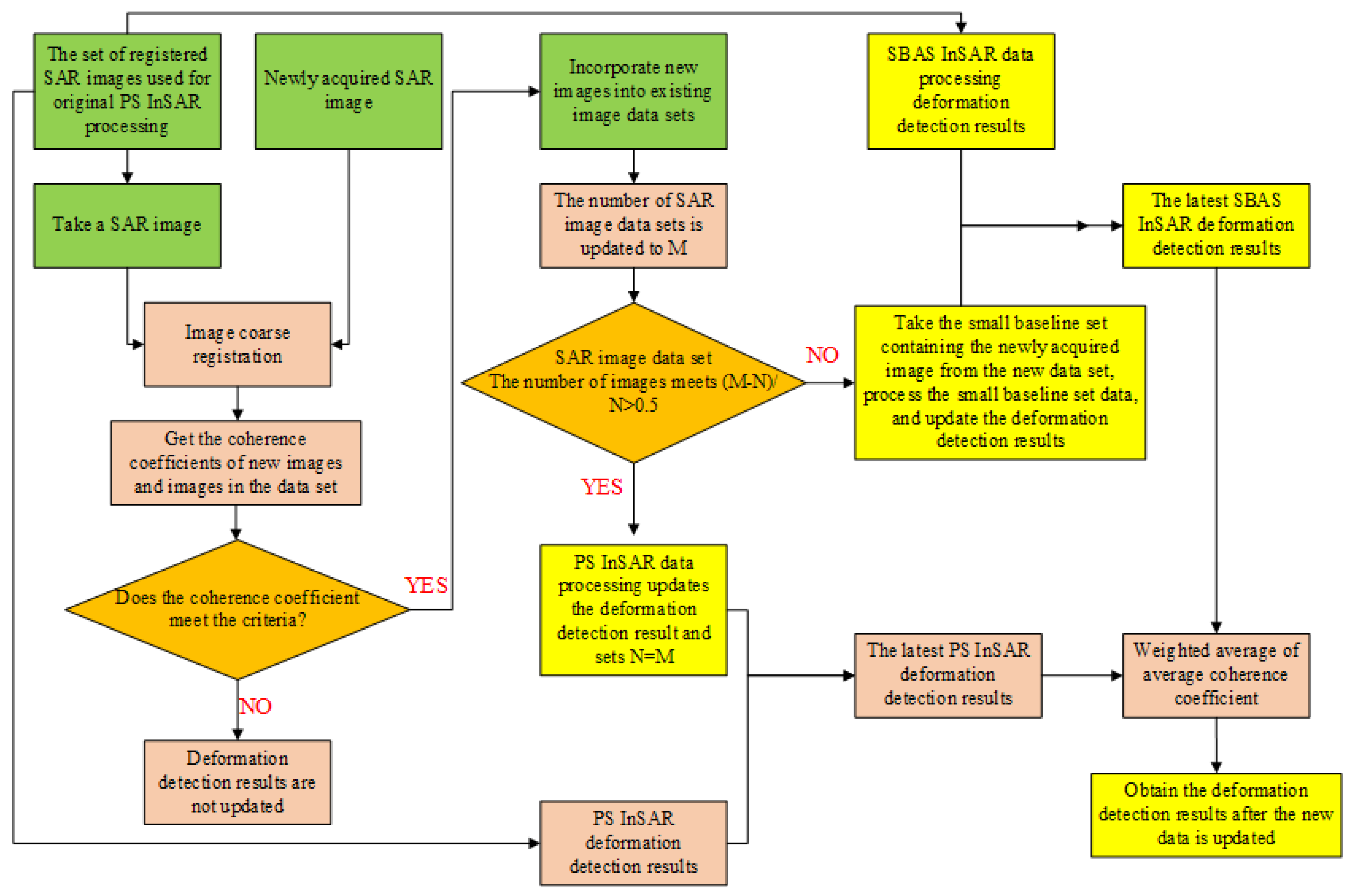
2.2. Proposed Method

The proposed method is divided into two parts. First, the Iterative Self-Organizing Data Analysis Techniques (ISODATA) algorithm is used to define the boundary between the slow subsidence region and the fast-subsidence region by clustering the distribution of land subsidence rates obtained by PS-InSAR. Second, when new SAR data are needed, SBAS-InSAR is used to efficiently develop small SAR data sets that include partial time-series SAR data and new SAR data. Moreover, the monitoring results are the sum of the latest results of SBAS-InSAR and the original result of the PS-InSAR for the time-series SAR datasets that are not included in the small SAR data sets. After updating with a certain amount of SAR data, the boundary and the monitoring results will be recalculated by PS-InSAR and SBAS-InSAR. The processed algorithm is partitioned into 10 steps, the procedure of which is shown in Figure 1.
Step 1: N SAR images are acquired from the SAR images set, for which N is more than or equivalent to 20, the SAR image set is defined as depicting the identical observation scenario, and the sets are aligned.
Step 2: The SAR image set derived in Step 1 is used in PS-InSAR for land settlement monitoring and to acquire the PSCs. The SBAS-InSAR also processes the SAR image set acquired in Step 1 to perform ground deformation monitoring and acquire the Slowly Decoherent Filtering Phase (SDFP) and the corresponding pixel coordinates.
Step 3: The acquired SAR image data are filtered and put into the image data set if they meet the filtering conditions. The primary screening condition involves calculating the coherence coefficient of the acquired image. If N1 of the calculated N coherence coefficient exceeds the predetermined threshold value p, then the alignment results satisfy the preset coherence conditions, where N1 > N × 0.6; P > 0.6.
Step 4: If the number M of images in the current image datasets meets the conditions (M − N)/N > 50%, go to Step 5, Otherwise, go to Step 6.
Step 5: PS-InSAR processing is performed on the image data from Step 4, the PS surface deformation results are calculated, the PS deformation results calculated in Step 2 are updated, and the maximum comprehensive coherence coefficient derived via PS-InSAR processing ρ 1 and the number of PS-InSAR images are updating, return to Step 3.
Step 6: N2 SAR images are selected from the image data set in Step 4 to form M1 small baseline sets and SBAS-InSAR processing is performed on the small baseline sets of the SAR image data newly acquired in Step 3 to obtain new SBAS surface deformation results, The average comprehensive coherence coefficient ρ 2 is updated.
Step 7: The ISODATA algorithm is used for the cluster analysis of the solution results derived in Step 6 to divide the deformation area and extract the most strongly developed region.
Step 8: The new SAR images of the strongly developed land subsidence area are acquired and screened again for SBAS-InSAR processing.
Step 9: The distribution of the accelerated land subsidence area is determined through the SBAS-InSAR monitoring results derived in Step 8.
Step 10: The SBAS deformation results from Step 6 and Step 8 are fused by the method of the weighted average for the accelerated land subsidence area. The PS deformation results from Step 5 and the SBAS deformation results from Step 8 are fused by the weighted average method for the slow land subsidence area. The weighted average method’s formula is as follows:
R = R 1 · w 1 + R 2 · w 2 / w 1 + w 2
where, R represents the fused land subsidence monitoring results, R1, and R2 indicate the ground settlement monitoring results of PS and SBAS-InSAR, separately, and w1 and w2 are weighting factors.

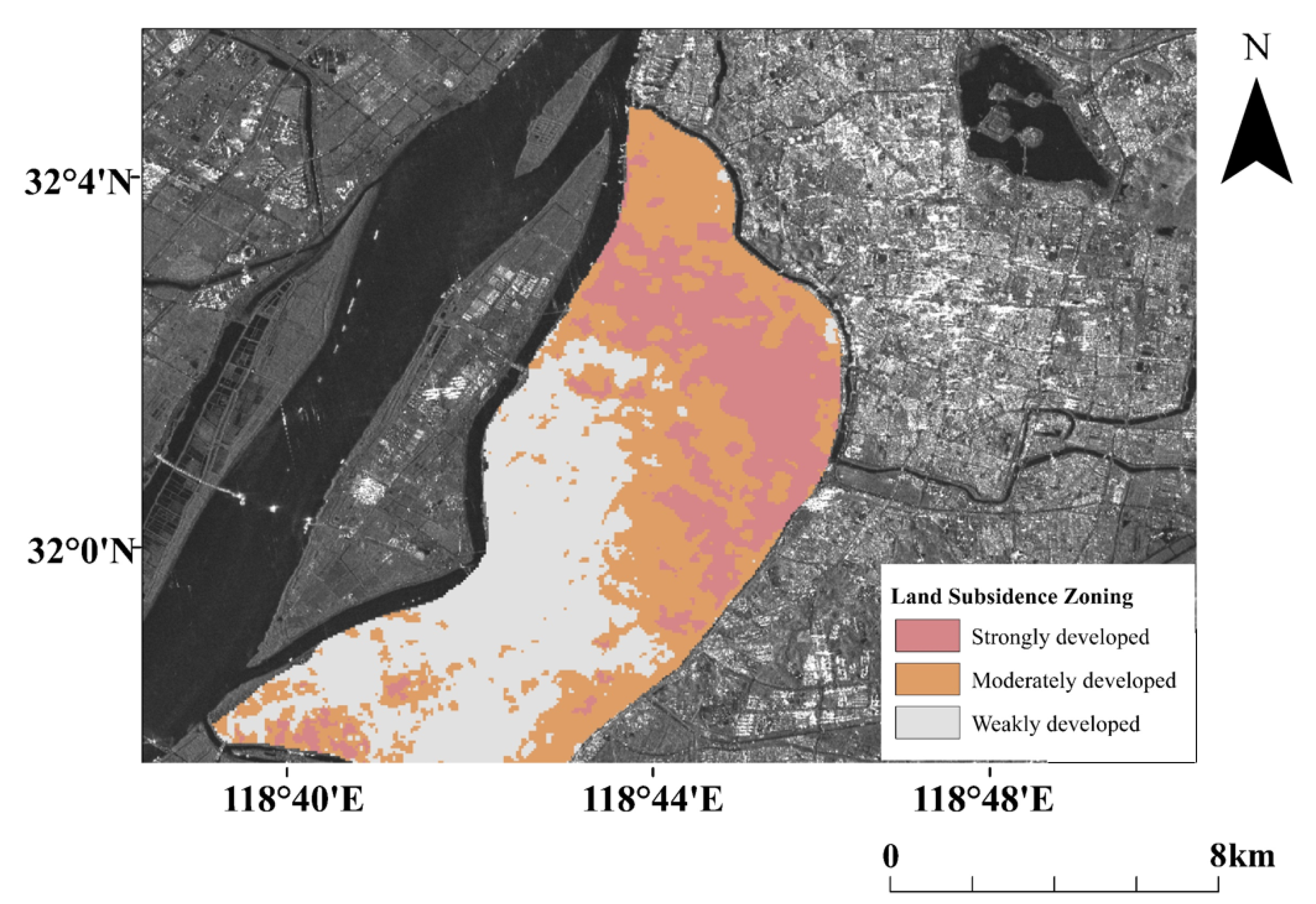
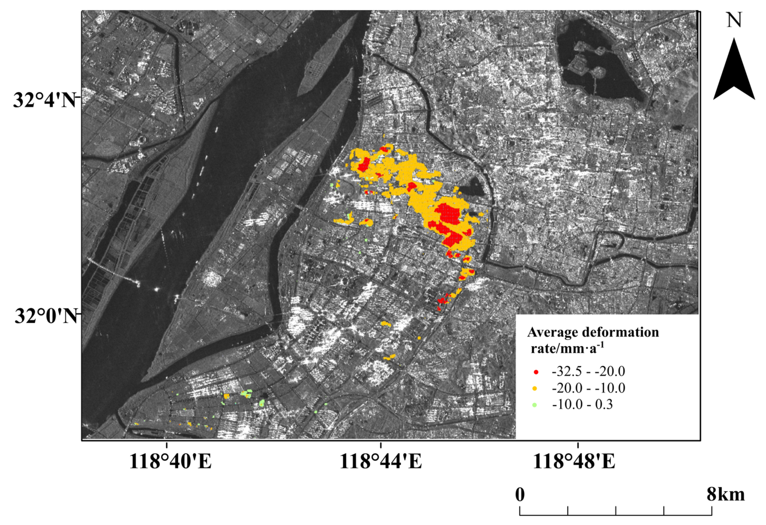
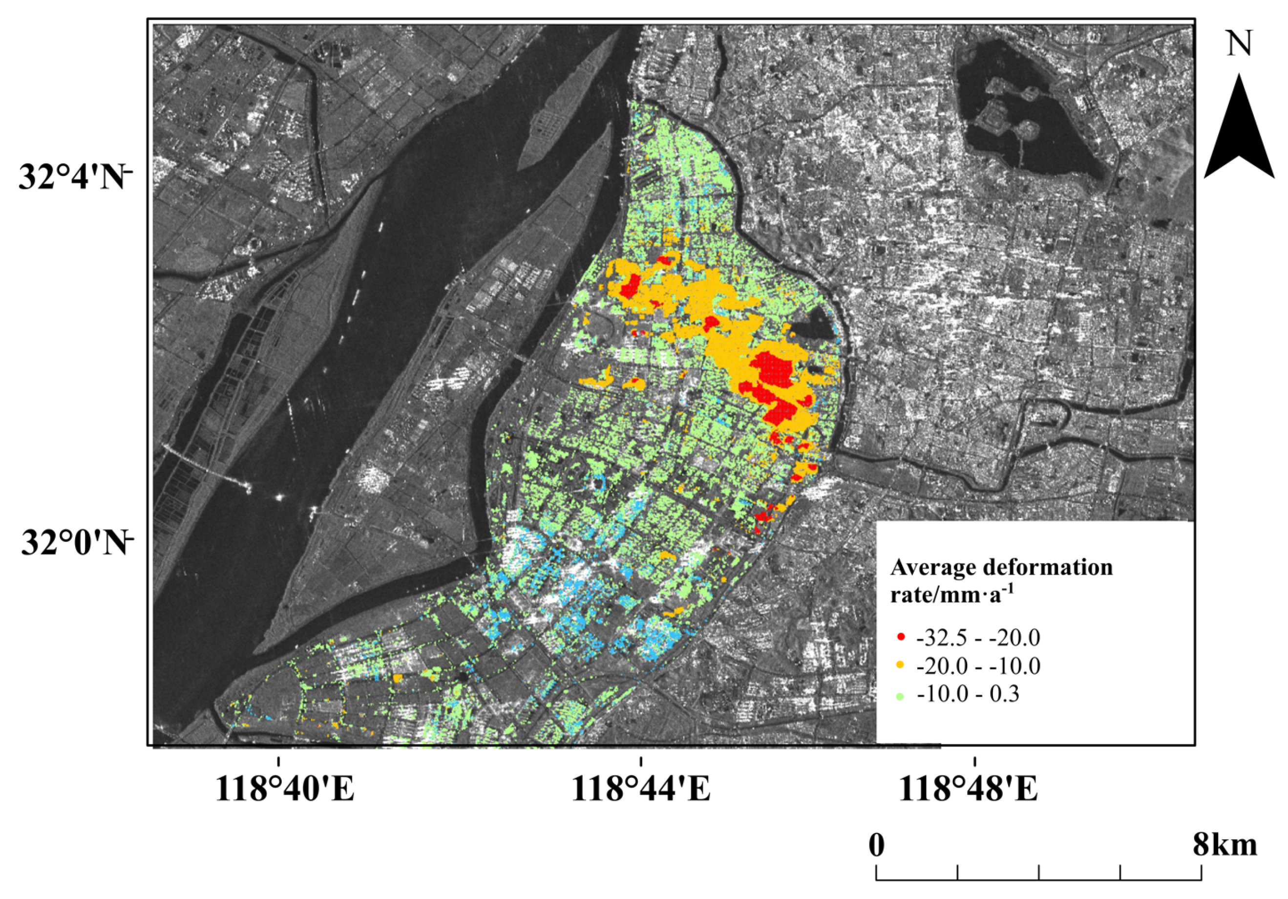
2.3. Land Settlement Rate Classification and Division

The ground settlement rate classification is an important basis for designing ground settlement monitoring networks and selecting ground settlement prevention methods. The principle of classifying strong and weak areas in this paper is that if the annual average settlement rate is less than 10 mm·a 1 , the area is classified as a weakly developed area of ground settlement, if the annual average land subsidence rate is between 10 and 30 mm·a 1 , the area is defined as a moderately developed area of ground settlement, and if the annual average land subsidence rate is ≥30 mm·a 1 , then the area is categorized as a strongly developed area of ground settlement, as listed in Table 1.
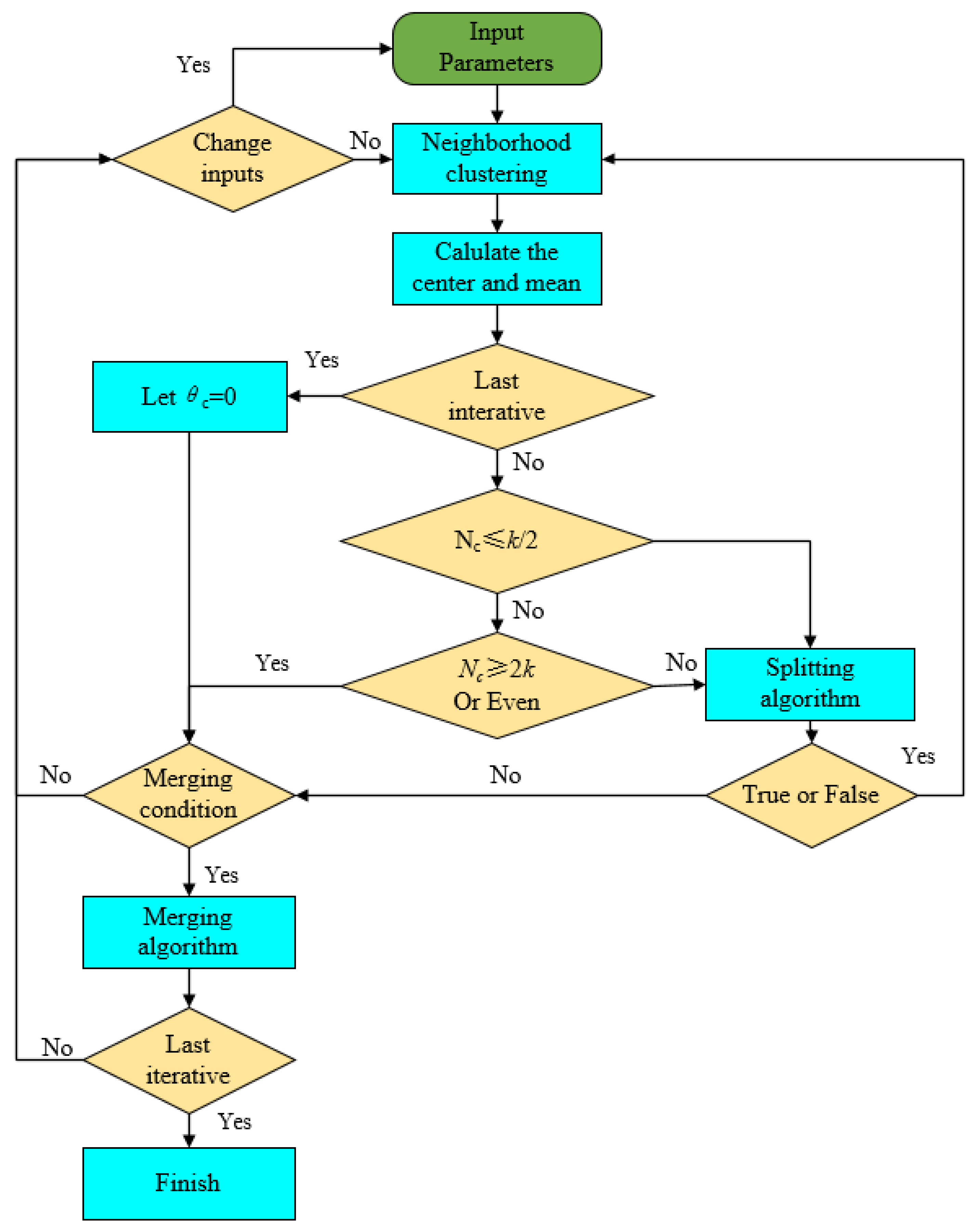
The ISODATA algorithm is a spatial clustering algorithm based on image segmentation and it is an unsupervised classification method. The ISODATA algorithm can use spatial information to identify and segment regions in images with highly similar target values and large differences between targets and achieve classification in a stepwise evolutionary manner. This study is used to classify land subsidence rates using three data layers simultaneously, such as SDFP, the corresponding pixel coordinates, and SABS InSAR-based ground subsidence values [46]. The ISODATA algorithm employs the following procedure [47]:
(1)
Select initial parameters.
(2)
Compute the distance index function for each of the clusters.
(3)
Merge or split clusters in accordance with the given requirements.
(4)
Loop iteration. Calculate the new index and define whether the result matches the clustering demands [47].
The ISODATA algorithm proceeds as follows, as shown in Figure 2:
Based on the unsupervised classification tool in the Arctoolbox of ArcGIS, the initial value N c of the clustering center can be chosen randomly and is set to 1 here. θ s , θ c and I are considered the default values for the ISODATA clustering algorithm in ArcGIS, θ n is given as 20, and the size of the neighborhood window R is a 20 × 20 grid. The input parameters are described in Table 2.

2.4. New SAR Data Filtering, Updating, and Integrating

Due to the high temporal and spatial sampling rate, SBAS-InSAR requires few satellite images, but generally, more than eight images, to ensure monitoring accuracy [6,48]. The fast-rate region can be searched for by applying SBAS-InSAR to small SAR data sets, including partial time-series SAR data and new SAR data from strongly developed ground deformation areas. To avoid the event of low coherence between the new SAR data and the original SAR data, the coherence coefficient is applied to screen the new SAR data.
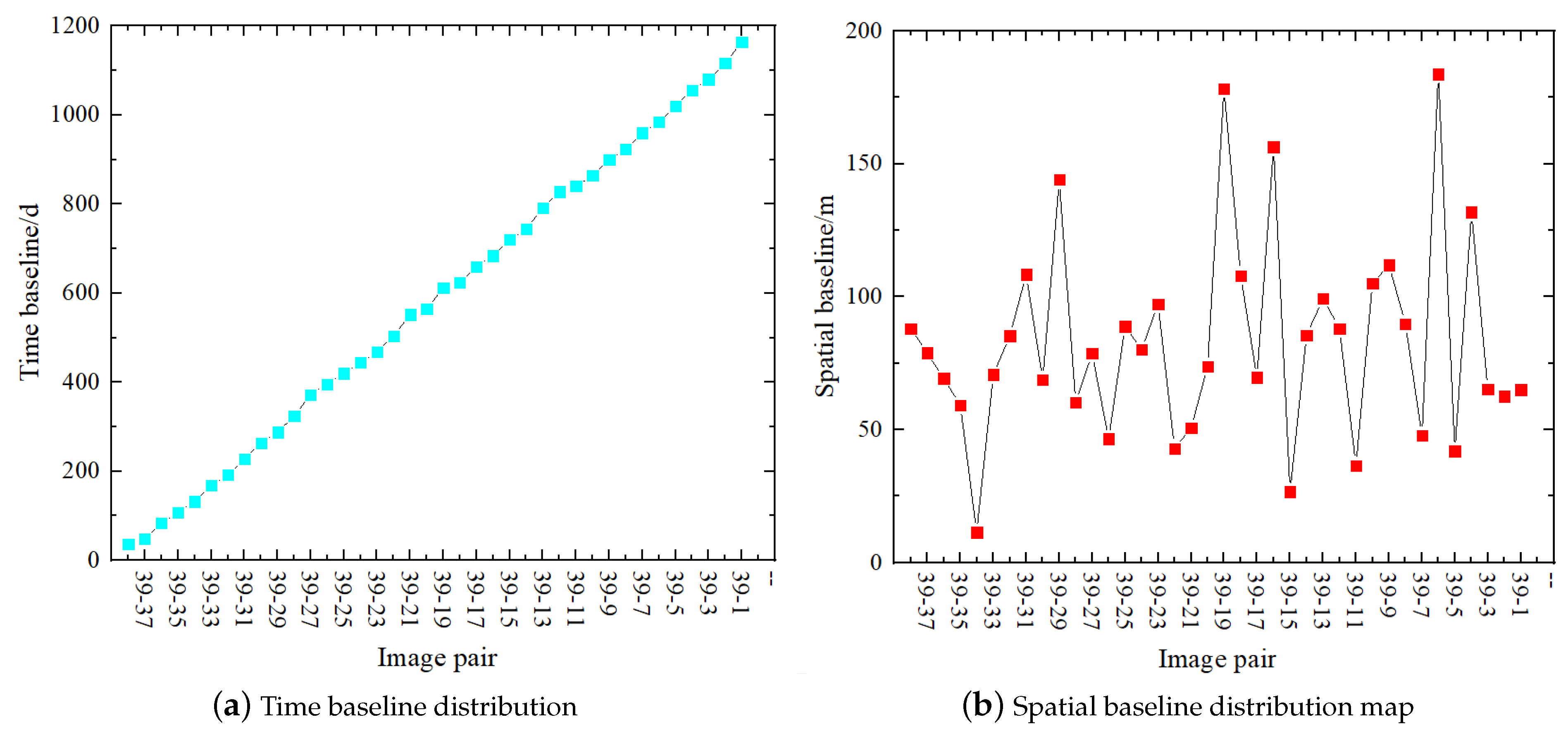
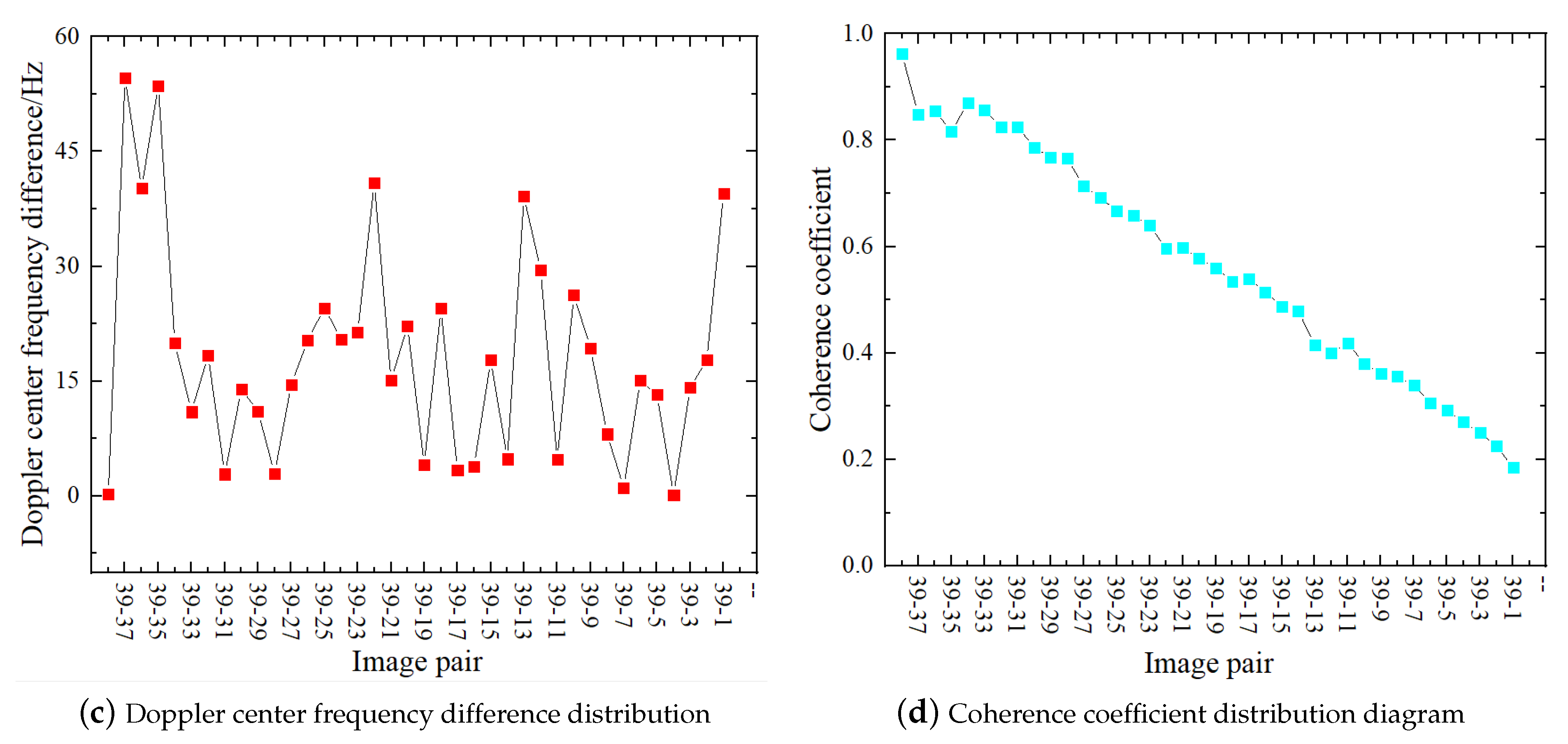
The maximum temporal resolution of the Sentinel-1A data is 12 days, with a critical time baseline of 4a, a critical Doppler center frequency difference of 486.486 Hz, and a critical spatial baseline of 6448 m. The screening criteria for the new SAR data are listed in Equations (7) and (8), and the master image is chosen according to the stacked coherence of the interferogram using Equation (7).
γ n , l = F B n , l , B c r × F T n , l , T m a x × F f d c n , l , f d c m a x
F x , α = 1 1 x α , x < α 0 , x > α
where n, l is the serial number of the master and slave images. T n , l represents a temporal baseline for the master and slave images. B n , l indicates the spatial baseline of the master and slave images. f d c n , l expresses the Doppler center frequency difference between the master and slave images. B c r indicates a critical effective baseline. T m a x is a critical temporal baseline. f d c m a x denotes the critical Doppler center frequency difference. N l is the set of images meeting the filtering criteria ( N l 8 ). γ n , l is the master-slave image coherence coefficient ( γ n , l 0.6 ) [32,49,50].
When the SDFPs from the SBAS-InSAR data set with higher spatial coverage are applied to the subsidence regions with rapid rates, two sets of SDFPs data are superimposed according to the sampling times of the two adjacent phases of SBAS-InSAR results, due to the different time scales of the two phases. The low-quality and low-density PSCs from the rapid-subsidence regions are removed from ArcGIS, and the updated SDFPs in the rapid-subsidence regions and the PSCs in the slow-subsidence regions are overlaid to obtain the fusion results for the areas of intensely different subsidence.

3. Case Study

3.1. Research Region

The research region is the western region of the Qinhuai River, Nanjing City, Jiangsu Province, China, which is located southwest of Nanjing’s main city, with the Qinhuai River, the South River, the Qinhuai New River, the Yangtze River, and the Sancha River to the southeast and northwest, respectively, and a land area of 56 km 2 , as seen in Figure 3. In the past decade, the accelerated urbanization of this research region has triggered regional ground deformation, and the differences in geological units, structural forms, and construction disturbances have caused drastic differences in ground deformation [51]. The LOS deformation from the tracks should be projected to the vertical. Meanwhile, considering the flat topography of the plain in this case study, the displacements obtained from InSAR (along the LOS direction) are directly interpreted as vertical deformations in this study.

3.2. SAR Datasets

The archived Sentinel-1A (2017–2020) datasets and the accessorial data from ALOS World’s three dimensions with 30 m resolution are used to evaluate ground surface settlement. The 38 images are contained within the interferometric wide-swath format, single-view complexes of the image pairs, together with the VV channels from https://scihub.esa.int/, (accessed on 1 June 2017) [14,35]. The primary parameters of the satellite systems are outlined in Table 3 [35].
In total, 38 images from the Sentinel-1A data set, covering the research area in the period from 2017.06 to 2020.07, have been chosen for both PS and SBAS-InSAR processing through the SARscape software. To be able to simultaneously satisfy the demands of PS and SBAS-InSAR calculations, the temporal-spatial baselines of the InSAR data sources had to be as small as reasonably possible. Two stacked C-band Sentinel-1A SAR data have been adopted for this study. The scenes are collected at a central frequency of 5.605 GHz (i.e., 5.6 cm wavelength, λ ) in the right-view mode and the Interferometric Width (IW) imaging modes. This was modeled on the Terrain Observation with Progressive Scans (TOPS) method, with the LOS incidence angle of 38.9 at the scene’s center. The IW imagery is characterized by a 250 km swath width, the use of the VV channel, and a 5 m ground distance and 20 m azimuth single-view resolution [6]. Sentinel-1A has wide coverage and a short revisit period of 12 days. After carefully identifying the track distribution of each SAR image, the SAR images of one month were picked for the experiments, the parameters of the interferometric wide (IW) TOPS acquisition mode and the experimental data are shown in Table 4 below.

4. Single Interferometry Procedure

4.1. PS-InSAR Processing

Master image are obtained from a 2D center consisting of temporal-spatial baselines during PS-InSAR processing (accessed on 22 February 2019). Then, 38 ascending Sentinel-1 images were co-aligned with the master image, moreover, a sum of 37 interferograms was derived from the data sets via interferometric processing. The produced spatial baselines were primarily distributed over the range of −130 m to −110 m, the longest spatial baseline was 121.802 m with a time baseline maximum of 600 d (Figure 4).
The first-order differential calculations for 37 interferograms is performed using the exact orbit of Sentinel-1A datasets to calculate the reference ellipsoidal phase and derive it from the original interferometric phases. The topographical phases are modeled with ALOS World three-dimension data and deduced from the first differential interference phase to achieve the interferometric phase images after two differential interference phases. The topographical phases are modeled with ALOS World 3D data and inferred from the first-order differential interference phase for obtaining the interferometric phase image following the two differential interference phases. To identify stable scattered targets, the coherence coefficient images exported from the interferometric processing are integrated with the amplitude images from the 38 Sentinel-1A data sets, furthermore, the minimum coherence threshold is fixed to 0.75 by the ADI method. The DEM correction coefficients and the average deformation rates of the candidate points are evaluated, and the atmospheric phases of PS candidate points are eliminated to obtain the final average deformation rate, as well as to gain the cumulative surface deformations, as shown in Figure 5.

4.2. SBAS-InSAR Processing

In the SBAS-InSAR technique, the algorithm is used to calculate the InSAR time-series according to a single-master network. First, the master image is picked by means of Equation (1) on the basis of the superimposed coherence of the interferogram. The superimposed coherence is an equation of the temporal baseline and the perpendicular spatial baseline. According to this process, the 2018-08-19 images are picked as the master image, and the temporal-spatial baseline thresholds are set after resampling all SLC image registrations (Figure 6). The experiment has a long-time span of roughly 38 months, and to decrease the adverse influence of orbital deviation, atmospheric delay, and topographic errors on the interferometric dataset generation, the temporal baseline length is bounded to 365 d and the spatial baseline length is limited to 645 m, which will yield 197 interferometric pairs.
Minimum cost flow (MCF) based on coherence calculation, flatting, filtering, and minimum phase unwrapping [52,53,54] have been tested on 272 interferometric pairs. Residual phase removal and Orbital refinement were applied to the unwrapping results, the orbital parameters were accurately estimated using GCP points, and the residual flat phase and orbit errors were deducted. In conjunction with the calculated high coherence point, a modeling solution has been derived to build the equations matrix, after which the elevation error and a linear deformation rate were evaluated by the matrix singular value decomposition (SVD) approach. The participating phases had to be separated, and the atmospheric phase composition of the residual phase was evaluated and removed from the residual phase. The de-correlation noise phases were eliminated with a filtering technique to derive the non-linear distorted phases. Eventually, the linear and non-linear deformation phases were superimposed to obtain the most accurate deformation results, as demonstrated in Figure 7.
As presented in Figure 5 and Figure 7, the annual mean deformation rates in the PS-InSAR monitoring results ranged from −24.3 to 24.5 mm·a 1 , while the annual average deformation rates in the SBAS-InSAR monitoring results varied from −32.1 to 19.8 mm·a 1 . The number of PSCs in the fast-subsidence region in the PS-InSAR monitoring results decreases as the subsidence rate increases until becoming incoherent. In the SBAS-InSAR monitoring results, the incoherence areas occur primarily where the subsidence rate is greater than 20 mm·a 1 . The regions of rapid subsidence are mainly located near the south of Mochou Lake, which should be monitored as a priority for residential areas and transport infrastructure.

5. Result

5.1. Land Subsidence Zoning Result

The ISODATA algorithm was used to derive the group of raster data in the multi-dimensional attribute space using the SBAS-InSAR monitoring results. The number of categories was set to 3 in the ISODATA algorithm. The zoning results derived using the ISODATA algorithm include weakly developed land subsidence areas, moderately developed land subsidence areas, and strongly developed land subsidence areas as shown in Figure 8. Strongly developed land subsidence mainly covers areas with land subsidence rates greater than 10 mm·a 1 , and moderately ground land subsidence areas occur in areas with land subsidence rates between approximately 0 and 10 mm·a 1 .

5.2. Searching for the Fast Rate of Land Subsidence Region

Sentinel-1 SAR data have been collected regularly in Nanjing, China, since June 2017. According to the Earth Data Center classification standard, the SAR data with the same path and boundary after 3 August 2020 has been selected. The results of multi-temporal InSAR processing show that the path number of the new SAR data is 69, the boundary number is 99, and the time stamp is 8 September 2020. Coherence coefficients are calculated for the new SAR data and the original SAR data, the results of which are shown in Figure 9. A total of 16 sets of SAR data with coherence coefficients greater than 0.6 satisfy the screening criteria. All original SAR data and new SAR data with coherence coefficients greater than 0.6 are merged to form a new data set Q and processed by SBAS-InSAR.
The number of PSCs in the fast-subsidence region in the PS-InSAR set decreases as the subsidence rate increases until becoming incoherent. Therefore, areas with subsidence rates greater than mm·a 1 are considered the fast-subsidence regions within the strongly developed ground settlement areas. Areas with subsidence rates more than 20 mm·a 1 , as monitored by two phases of SBAS-InSAR are plotted in the zoning map of ground subsidence, as depicted in Figure 10. Answer: We confirmed.
The red area is the region with a subsidence rate greater than 20 mm·a 1 . Compared with the two adjacent phases of SBAS-InSAR results, there is a clear trend of expansion in the red area, which indicates a rapid rate of subsidence in the area of strongly developed ground subsidence. SBAS-InSAR can search for areas with settling rates greater than 20 mm·a 1 via the continuous monitoring of fast-settling areas.

5.3. Data Update and Integrate

The time span of dataset N is from 2 July 2017 to 3 August 2020, and the time span of data set Q is from 29 May 2019 to 8 September 2020. Since the time node of fusion is determined by the temporal beginning of the new image data set, 29 May 2019 is used as the node to fuse the two sets of SDFP pixel data and update the SDFP pixels in the subsidence region at a rapid rate. The results are given in Figure 11. The highest subsidence rate after the data update is 32.5 mm·a 1 , which is slightly higher than the 32.1 mm·a 1 shown in Figure 7. This is because the time interval of only one new image phase is updated, and the variation in the annual average subsidence rate is relatively small. Answer: We confirmed.
Figure 12 shows the maximum annual average subsidence rate increased from 32.1 mm·a 1 to 32.5 mm·a 1 as a result of the continuous monitoring of rapid-subsidence regions in highly developed ground subsidence areas. In addition, the maximum uplift rate decreased from 24.5 mm·a 1 to 10.5 mm·a 1 due to the removal of misclassified uplift PSCs from the accelerated settlement region after the adoption of SDFP pixel points.

6. Discussion

6.1. Pixel Points Variation Pattern in Land Subsidence

The statistical analysis of the PSCs yielded by PS-InSAR and the SDFPs yielded by SBAS-InSAR indicates that there are 86,578 PSCs and 149,366 SDFPs, and the total number of SDFPs is much greater than that of PSCs. The maximum deformation rates in the LOS direction for the PS and SDFP pixel points are −12 and −7 mm·a 1 , respectively. Meanwhile, the frequency distribution pattern of the PS and SDFP pixel points is more similar in terms of the values of the deformation rates, as displayed in Figure 13.
The 2761 PSCs and SDFPs with the same geographical coordinates in the research region have been screened, and the correlation analysis of the subsidence rates at the screened points indicates, that the linear correlation coefficient R exceeds reaches above 0.93, as displayed in Figure 14.

6.2. Time-Series Analysis of Land Subsidence

After comparing the variation in cumulative land subsidence over time in areas showing rapid land subsidence, characteristic points in the regions 0~10 mm·a 1 , 10~20 mm·a 1 , and 20~30 mm·a 1 has been selected for plotting the time-series variation curves of cumulative land subsidence, where the characteristic points A1 and A2 are located in the region with a land subsidence rate of 20~30 mm·a 1 . In addition, the characteristic points B1 and B2 are located in the region with a land subsidence rate of 10~20 mm·a 1 , and C1 and C2 are located in the region with a land subsidence rate of 0~10 mm·a 1 , as shown in Figure 15. The time-series variation profiles of accumulated subsidence at the feature points over set time are presented in Figure 16. The deviations in the accumulated subsidence monitoring values given by the two techniques have also been statistically analyzed.
From Figure 16, we see that the two monitoring technologies identified a sharp increase in the cumulative settlement at feature point C as time proceeded, and their trends are relatively comparable. When the density of PS points decreases, PS-InSAR’s removal of the atmospheric phase will produce relatively large errors, and at this time, SBAS-InSAR’s results can complement the PS-InSAR monitoring values. The time-series analysis results and the deviation statistics are shown in Table 5. In the region with land subsidence rates of 0~10 mm·a 1 , the cumulative land subsidence deviations of PS- and SBAS-InSAR were −0.7 and 0.6, respectively. The deviations in cumulative land subsidence between PS- and SBAS-InSAR were, respectively, found to be −1.1 and 1.7 in the region with subsidence rates of 10~20 mm·a 1 . In the region with the land subsidence rates of 20~30 mm·a 1 , the deviations of the cumulative land subsidence between PS- and SBAS-InSAR were, respectively, 5.6 and 4.0. In summary, as the land subsidence rate increased, the deviation also increases due to the loss of coherence caused by the dramatic land subsidence in the fast-subsidence region.
The numbers of PSCs and SDFPs in the fast-subsidence regions are shown in Table 6. In the regions with rapid subsidence rates, there are 4036 low-quality and low-density PSCs and 15,667 updated SDFPs. Simultaneously, the density of monitoring points increased from 711/km 2 to 2760/km 2 , an increase of 288.2%. In other regions, because of the low ground subsidence rate and high feature coherence, the density of existing PS points meets the demands of high precision in land subsidence monitoring. The data fusion results in the more rational deployment of monitoring points, thus significantly increasing the density of monitoring points in areas of accelerated subsidence and precluding misclassified uplift monitoring points. The method in this paper makes full use of all satellite observations while improving monitoring efficiency, enabling the timely capturing of accelerated subsidence areas within strongly developed ground settlement areas and the continuous monitoring of accelerated deformation areas.
Even though the PS-SBAS integration results in this study are encouraging, a large error of more than 1 cm/year still occurs in certain regions of the research region. The results from existing continuous GPS stations in these regions may reduce these large errors. The concept is to model atmospheric delays using continuous GPS measurements and subsequently apply the GPS measurements to regulate the atmospheric impacts within radar interferograms.

6.3. Induced Causes of Land Subsidence

Many prior studies have adequately documented the exploration of land subsidence and the triggering factors in Southeast regions of China, which also lie in the southern part of Jiangsu Province, around the lower reaches of the Yangtze River, and east of Shanghai City. These regions have various types of groundwater, an uneven distribution of groundwater, and complex burial conditions, with distinctive regional characteristics. It was found that the Suzhou-Wuxi-Changzhou area has suffered severe land subsidence due to long-term excessive exploitation, ground fissure activity and pumping [55,56]. Based on long-term measurement data, the uneven land subsidence and the differential settlement of infrastructure in Shanghai were caused by groundwater exploitation and artificial recharge in an alternated multi-aquifer-aquitard system [57]. In most cases, the pattern of land subsidence might be even more complicated when it is induced by a combination of multiple factors at different scales. This paper focused on groundwater exploitation and the industry or underground construction, along with the effects on the spatio-temporal changes of groundwater exploitation and ground displacements. However, considering the complexity of the land use and the geological conditions in different districts of Nanjing City, the land subsidence may not be only induced by groundwater extraction and surface construction, but also by the integrated factors of numerous natural situations and anthropogenic processes. Therefore, future work should include a more comprehensive analysis of triggering factors to remove some of the limitations of this study.

7. Conclusions

This paper proposes a new land subsidence monitoring algorithm, formed by fusing PS-InSAR and SBAS-InSAR interferometric data from zones with differential land subsidence rates. This integrated method can ensure the accuracy and efficiency of data updates and InSAR calculation, and address the low local accuracy of using single interferometry to assess differential land subsidence in an urban center.
The SDFPs are acquired by SBAS-InSAR, and the land subsidence rates of the SDFPs are clustered and analyzed using the ISODATA algorithm to identify the most strongly developed ground subsidence areas. The new SAR data in the strongly developed ground land subsidence areas are obtained and filtered, and then SBAS-InSAR processing is performed again. Meanwhile, the results of the second phase of SBAS-InSAR monitoring are applied to rapidly determine the subsidence region. Finally, the SBAS-InSAR data of two phases are fused for the fast-subsidence region, and PS-InSAR monitoring data are adopted for the slow-subsidence region. The monitoring results are the sum of the latest results of SBAS-InSAR and the original results derived from PS-InSAR or SBAS-InSAR taken from the temporal region of SAR data which is not included in the small SAR data set. Application of the western area of the Qinhuai River, Nanjing, China has indicated that the proposed method eliminates the PSCs, reducing the monitoring accuracy in the fast-subsidence region. When the SDFPs are used in the fast-subsidence region, the density of monitoring points significantly increases from 711 points/km 2 to 2760 points/km 2 —an increase of 288.2%.
The engineering case indicates that the integrated method can take full advantage of the validity of all satellite observations and fuses the main advantages of these two monitoring techniques to improve the efficiency of monitoring in regions with different subsidence rates. By promptly capturing accelerated settlement areas within regions of strongly developed ground settlement, the accelerated settlement rate is efficiently tracked, and the settlement areas can be closely monitored.

Author Contributions

P.Z.: Supervision, Conceptualization, Methodology, Funding acquisition X.Q.: Investigation, Data curation, Software, Writing-original draft. S.G.: Methodology, Software, Writing-original draft, Visualization. B.W.: Writing-review & editing, Funding acquisition. J.X.: Formal analysis, Data curation. X.Z.: Supervision, Validation, Writing-review & editing. All authors have read and agreed to the published version of the manuscript.

Funding

The paper was support by the National Nature Science Foundation of China (NSFC NO. 41372295 and NO. 41102178); the Fellowship of China Postdoctoral Science Foundation (NO. 2021M701688); outstanding Postdoctoral Fellowship of Jiangsu Foundation (NO. 283762); Open Fund of Shaanxi Key Laboratory of Geotechnical and Underground Space Engineering (NO. YT202201); carbon Peak Carbon Neutral Technology Innovation Special of Jiangsu Foundation (BE2022605).

Conflicts of Interest

The authors declare no conflict of interest.

References

  1. Yu, H.; Gong, H.; Chen, B.; Liu, K.; Gao, M. Analysis of the influence of groundwater on land subsidence in Beijing based on the geographical weighted regression (GWR) model. Sci. Total Environ. 2020, 738, 139405. [Google Scholar] [CrossRef] [PubMed]
  2. Pu, C.; Xu, Q.; Zhao, K.; Chen, W.; Wang, X.; Li, H.; Liu, J.; Kou, P. Spatiotemporal evolution and the surface response of land subsidence over a large-scale land creation area on the Chinese Loess Plateau. Int. J. Appl. Earth Obs. Geoinf. 2022, 111, 102835. [Google Scholar] [CrossRef]
  3. Shi, W.; Chen, G.; Meng, X.; Jiang, W.; Chong, Y.; Zhang, Y.; Dong, Y.; Zhang, M. Spatial-temporal evolution of land subsidence and rebound over Xi’an in western china revealed by SBAS-InSAR analysis. Remote Sens. 2020, 12, 3756. [Google Scholar] [CrossRef]
  4. Shi, G.; Ma, P.; Hu, X.; Huang, B.O.; Lin, H. Surface response and subsurface features during the restriction of groundwater exploitation in Suzhou inferred from decadal SAR interferometry. Remote Sens. Environ. 2021, 256, 112327. [Google Scholar] [CrossRef]
  5. Miranda, S.F.; Hernández-Madrigal, V.M.; Tuxpan-Vargas, J.; Reyes, C.I.V. Evolution assessment of structurally-controlled differential subsidence using SBAS and PS interferometry in an emblematic case in Central Mexico. Eng. Geol. 2020, 279, 105860. [Google Scholar] [CrossRef]
  6. Cigna, F.; Esquivel Ramírez, R.; Tapete, D. Accuracy of Sentinel-1 PSI and SBAS InSAR Displacement Velocities against GNSS and Geodetic Leveling Monitoring Data. Remote Sens. 2021, 13, 4800. [Google Scholar] [CrossRef]
  7. Dehghani, M.; Zoej, M.; Hooper, A. Hybrid conventional and Persistent Scatterer SAR interferometry for land subsidence monitoring in the Tehran Basin, Iran. ISPRS J. Photogramm. Remote Sens. 2013, 79, 157–170. [Google Scholar] [CrossRef]
  8. Corbau, C.; Simeoni, U.; Zoccarato, C.; Mantovani, G.; Teatini, P. Coupling land use evolution and subsidence in the Po Delta, Italy: Revising the past occurrence and prospecting the future management challenges. Sci. Total Environ. 2019, 654, 1196–1208. [Google Scholar] [CrossRef]
  9. Hu, L.; Dai, K.; Xing, C.; Li, Z.; Tomas, R.; Clark, B.; Shi, X.; Chen, M.i.; Zhang, R.; Qiu, Q.; et al. Land subsidence in Beijing and its relationship with geological faults revealed by Sentinel-1 InSAR observations. Int. J. Appl. Earth Obs. Geoinf. 2019, 82, 101886. [Google Scholar] [CrossRef]
  10. Zhou, C.; Gong, H.; Chen, B.; Li, J.; Gao, M.; Zhu, F.; Chen, W.; Liang, Y. InSAR time-series analysis of land subsidence under different land use types in the eastern Beijing Plain, China. Remote Sens. 2017, 9, 380. [Google Scholar] [CrossRef] [Green Version]
  11. Peng, M.; Zhao, C.; Zhang, Q.; Lu, Z.; Li, Z. Research on spatial-temporal land deformation (2012–2018) over Xi’an, China, with Multi-Sensor SAR Datasets. Remote Sens. 2019, 11, 664. [Google Scholar] [CrossRef] [Green Version]
  12. Hooper, A. A multi-temporal InSAR method incorporating both persistent scatterer and small baseline approaches. Geophys. Res. Lett. 2008, 35, 96–106. [Google Scholar] [CrossRef] [Green Version]
  13. Reinisch, E.; Cardiff, M.; Feigl, K. Graph theory for analyzing pair-wise data: Application to geophysical model parameters estimated from interferometric synthetic aperture radar data at Okmok volcano, Alaska. J. Geod. 2017, 91, 9–24. [Google Scholar] [CrossRef] [PubMed] [Green Version]
  14. Zhao, K.; Wang, Q.; Zhuang, H.; Li, Z.; Chen, G. A fully coupled flow deformation model for seismic site response analyses of liquefiable marine sediments. Ocean Eng. 2022, 251, 111144. [Google Scholar] [CrossRef]
  15. Werner, W.; Freysteinn, S.; Stéphanie, D.; Lavallée, Y. Post-emplacement cooling and contraction of lava flows: InSAR observations and a thermal model for lava fields at Hekla volcano, Iceland. J. Geophys. Res.-Solid Earth 2017, 122, 946–965. [Google Scholar] [CrossRef] [Green Version]
  16. Foroughnia, F.; Nemati, S.; Maghsoudi, Y.; Perissin, D. An iterative PS-InSAR method for the analysis of large spatio-temporal baseline data stacks for land subsidence estimation. Int. J. Appl. Earth Obs. Geoinf. 2019, 74, 248–258. [Google Scholar] [CrossRef]
  17. Luo, H.; Li, Z.; Chen, J.; Pearson, C.; Wang, M.; Lv, W.; Ding, H. Integration of Range Split Spectrum Interferometry and conventional InSAR to monitor large gradient surface displacements. Int. J. Appl. Earth Obs. Geoinf. 2019, 74, 130–137. [Google Scholar] [CrossRef] [Green Version]
  18. Lanari, R.; Bonano, M.; Casu, F.; De Luca, C.; Manunta, M.; Manzo, M.; Onorato, G.; Zinno, I. Automatic generation of Sentinel-1 continental scale DInSAR deformation time series through an extended P-SBAS processing pipeline in a cloud computing environment. Remote Sens. 2020, 12, 2961. [Google Scholar] [CrossRef]
  19. Botey i Bassols, J.; Vàzquez-Suñé, E.; Crosetto, M.; Barra, A.; Pierre, G. D-InSAR monitoring of ground deformation related to the dewatering of construction sites. A case study of Glòries Square, Barcelona. Eng. Geol. 2021, 286, 106041. [Google Scholar] [CrossRef]
  20. Ferretti, A.; Prati, C.; Rocca, F. Permanent scatterers in SAR interferometry. IEEE Trans. Geosci. Remote Sens. 2001, 39, 8–20. [Google Scholar] [CrossRef]
  21. Hooper, A.; Zebker, H.; Segall, P.; Kampes, B. A new method for measuring deformation on volcanoes and other natural terrains using InSAR persistent scatterers. Geophys. Res. Lett. 2004, 31, 1–5. [Google Scholar] [CrossRef]
  22. Hooper, A.; Segall, P.; Zebker, H.A. Persistent scatterer interferometric synthetic aperture radar for crustal deformation analysis, with application to Volcan Alcedo, Galapagos. J. Geophys. Res.-Solid Earth 2007, B07407, 112. [Google Scholar] [CrossRef] [Green Version]
  23. López-Quiroz, P.; Doin, M.P.; Tupin, F.; Briole, P.; Nicolas, J.M. Time series analysis of Mexico City subsidence constrained by radar interferometry. J. Appl. Geophys. 2009, 69, 1–15. [Google Scholar] [CrossRef]
  24. Hetland, E.A.; Musã, P.; Simons, M.; Lin, Y.N.; Agram, P.S.; Dicaprio, C.J. Multiscale InSAR Time Series (MInTS) analysis of surface deformation. J. Geophys. Res. 2012, 117, B02404. [Google Scholar] [CrossRef] [Green Version]
  25. Chen, M.; Tomás, R.; Li, Z.; Motagh, M.; Li, T.; Hu, L.; Gong, H.; Li, X.; Yu, J.; Gong, X. Imaging land subsidence induced by groundwater extraction in Beijing (China) using satellite radar interferometrys. Remote Sens. 2016, 8, 468. [Google Scholar] [CrossRef] [Green Version]
  26. Motagh, M.; Shamshiri, R.; Haghighi, M.H. Quantifying groundwater exploitation induced subsidence in the Rafsanjan plain, southeastern Iran, using InSAR time-series and in situ measurements. Eng. Geol. 2017, 218, 134–151. [Google Scholar] [CrossRef]
  27. Samsonov, S.; Dille, A.; Dewitte, O.; Kervyn, F.; d’Oreye, N. Satellite interferometry for mapping surface deformation time series in one, two and three dimensions: A new method illustrated on a slow-moving landslide. Eng. Geol. 2020, 266, 105471. [Google Scholar] [CrossRef]
  28. Bui, L.K.; Featherstone, W.E.; Filmer, M.S. Disruptive influences of residual noise, network configuration and data gaps on InSAR-derived land motion rates using the SBAS technique. Remote Sens. Environ. 2020, 247, 111941. [Google Scholar] [CrossRef]
  29. Berardino, P.; Fornaro, G.; Lanari, R.; Sansosti, E. A New Algorithm for Surface Deformation Monitoring Based on Small Baseline Differential SAR Interferograms. IEEE Trans. Geosci. Remote Sens. 2002, 40, 2375–2383. [Google Scholar] [CrossRef] [Green Version]
  30. Bateson, L.; Cigna, F.; Boon, D.; Sowter, A. The application of the inter-mittent SBAS (ISBAS) InSAR method to the south wales coalfield, UK. Int. J. Appl. Earth Obs. Geoinf. 2015, 34, 249–257. [Google Scholar] [CrossRef] [Green Version]
  31. Chen, H.; Zhao, C.; Li, B.; Chen, L.; Liu, D. Monitoring spatiotemporal evolution of Kaiyang landslides induced by phosphate mining using distributed scatterers InSAR technique. Landslides 2023, 20, 695–706. [Google Scholar] [CrossRef]
  32. Maghsoudi, Y.; Meer, F.; Hecker, C.; Perissin, D.; Saepuloh, A. Using PS-InSAR to detect surface deformation in geothermal areas of West Java in Indonesia. Int. J. Appl. Earth Obs. Geoinf. 2018, 64, 386–396. [Google Scholar] [CrossRef]
  33. Maghsoudi, Y.; Amani, R.; Ahmadi, H. A study of land subsidence in west of Tehran using Sentinel-1 data and permanent scatterer interferometric technique. Arab. J. Geosci. 2021, 14, 30. [Google Scholar] [CrossRef]
  34. Khan, R.; Li, H.; Afzal, Z.; Basir, M.; Hassan, W. Monitoring Subsidence in Urban Area by PSInSAR: A Case Study of Abbottabad City, Northern Pakistan. Remote Sens. 2021, 13, 1651. [Google Scholar] [CrossRef]
  35. Zhang, P.; Guo, Z.; Guo, S.; Xia, J. Land Subsidence Monitoring Method in Regions of Variable Radar Reflection Characteristics by Integrating PS-InSAR and SBAS-InSAR Techniques. Remote Sens. 2022, 14, 3265. [Google Scholar] [CrossRef]
  36. Shanker, P.; Casu, F.; Zebker, H.A.; Lanari, R. Comparison of Persistent Scatterers and Small Baseline Time-Series InSAR Results: A Case Study of the San Francisco Bay Area. IEEE Geosci. Remote Sens. Lett. 2011, 8, 592–596. [Google Scholar] [CrossRef]
  37. Crosetto, M.; Monserrat, O.; Cuevas-Gonzalez, M.; Devanthery, N.; Crippa, B. Persistent Scatterer Interferometry: A review. ISPRS J. Photogramm. Remote Sens. 2016, 115, 78–89. [Google Scholar] [CrossRef] [Green Version]
  38. Wei, T.; Mahdi, M.; Wei, Z. Monitoring active open-pit mine stability in the Rhenish coalfields of Germany using a coherence-based SBAS method. Int. J. Appl. Earth Obs. Geoinf. 2020, 93, 102217. [Google Scholar] [CrossRef]
  39. Du, Z.Y.; Ge, L.L.; Ng, A.H.M.; Zhu, Q.G.Z.; Horgan, F.G.; Zhang, Q. Risk assessment for tailings dams in Brumadinho of Brazil using InSAR time series approach. Sci. Total Environ. 2020, 717, 137125. [Google Scholar] [CrossRef]
  40. Chen, Y.; Yu, S.; Tao, Q.; Liu, G.; Wang, L.; Wang, F. Accuracy Verification and Correction of D-InSAR and SBAS-InSAR in Monitoring Mining Surface Subsidence. Remote Sens. 2021, 13, 4365. [Google Scholar] [CrossRef]
  41. Aslan, G.; Foumelis, M.; Raucoules, D.; Michele, M.D.; Bernardie, S.; Cakir, Z. Landslide mapping and monitoring using persistent scatterer interferometry (PSI) technique in the French Alps. Remote Sens. 2021, 12, 1305. [Google Scholar] [CrossRef] [Green Version]
  42. Tarighat, F.; Foroughnia, F.; Perissin, D. Monitoring of Power Towers’ Movement Using Persistent Scatterer SAR Interferometry in South West of Tehran. Remote Sens. 2021, 13, 407. [Google Scholar] [CrossRef]
  43. Guo, C.B.; Yan, Y.Q.; Zhang, Y.S.; Zhang, X.J.; Zheng, Y.Z.; Li, X.; Yang, Z.H.; Wu, R. Study on the Creep-Sliding Mechanism of the Giant Xiongba Ancient Landslide Based on the SBAS-InSAR Method, Tibetan Plateau, China. Remote Sens. 2021, 13, 3365. [Google Scholar] [CrossRef]
  44. Liu, L.M.; Yu, J.; Chen, B.B.; Wang, Y.B. Urban subsidence monitoring by SBAS-InSAR technique with multi-platform SAR images: A case study of Beijing Plain, China. Eur. J. Remote Sens. 2020, 53, 2279–7254. [Google Scholar] [CrossRef] [Green Version]
  45. Wu, Q.; Jia, C.T.; Chen, S.B.; Li, H.Q. SBAS-InSAR Based Deformation Detection of Urban Land, Created from Mega-Scale Mountain Excavating and Valley Filling in the Loess Plateau: The Case Study of Yan’an City. Remote Sens. 2019, 11, 1673. [Google Scholar] [CrossRef] [Green Version]
  46. Zhang, P.; Qian, X.; Guo, X.; Yang, X.; Li, G. Automated demarcation of the homogeneous domains of trace distribution within a rock mass based on GLCM and ISODATA. Int. J. Rock Mech. Min. Sci. 2020, 128, 104249. [Google Scholar] [CrossRef]
  47. Zhang, P.; Li, J.; Yang, X.; Zhu, H. Semi-automatic extraction of rock discontinuities from point clouds using the ISODATA clustering algorithm and deviation from mean elevation. Int. J. Rock Mech. Min. Sci. 2018, 128, 76–87. [Google Scholar] [CrossRef]
  48. Yuan, M.; Li, M.; Liu, H.; Lv, P.; Li, B.; Zheng, W. Subsidence Monitoring Base on SBAS-InSAR and Slope Stability Analysis Method for Damage Analysis in Mountainous Mining Subsidence Regions. Remote Sens. 2021, 13, 3107. [Google Scholar] [CrossRef]
  49. Zhou, C.; Cao, Y.; Yin, K.; Wang, Y.; Shi, X.; Catani, F.; Ahmed, B. Landslide Characterization Applying Sentinel-1 Images and InSAR Technique: The Muyubao Landslide in the Three Gorges Reservoir Area, China. Remote Sens. 2020, 12, 3385. [Google Scholar] [CrossRef]
  50. Kampes, B.M. Radar Interferometry: Persistent Scatterer Technique; Springer: Dordrecht, The Netherlands, 2006. [Google Scholar] [CrossRef]
  51. Yang, Z.; Xu, J. Monitoring the land subsidence in Hexi area of Nanjing by using Sentinel-1A. Bull. Surv. Mapp. 2020, 61–65+75. [Google Scholar] [CrossRef]
  52. Darwish, N.; Kaiser, M.; Koch, M.; Gaber, A. Assessing the accuracy of ALOS/PALSAR-2 and sentinel-1 radar images in estimating the land subsidence of coastal areas: A case study in Alexandria city, Egypt. Remote Sens. 2021, 13, 1838. [Google Scholar] [CrossRef]
  53. He, Y.; Xu, G.; Kaufmann, H.; Wang, J.; Ma, H.; Liu, T. Integration of InSAR and LiDAR Technologies for a Detailed Urban Subsidence and Hazard Assessment in Shenzhen, China. Remote Sens. 2021, 13, 2336. [Google Scholar] [CrossRef]
  54. Cigna, F.; Tapete, D. Satellite InSAR survey of structurally-controlled land subsidence due to groundwater exploitation in the Aguascalientes Valley. Remote Sens. Environ. 2021, 254, 2254. [Google Scholar] [CrossRef]
  55. Xu, J.; Peng, J.; An, H. Experimental study on Su-Xi-Chang earth fissures induced by repeated groundwater pumping and impounding. Geomat. Nat. Hazards Risk 2019, 10, 2051–2068. [Google Scholar] [CrossRef] [Green Version]
  56. Yang, C.; Lv, S.; Hou, Z.; Zhang, Q.; Li, T.; Zhao, C. Monitoring of Land Subsidence and Ground Fissure Activity within the Su-Xi-Chang Area Based on Time-Series InSAR. Remote Sens. 2022, 14, 903. [Google Scholar] [CrossRef]
  57. Li, M.; Chen, J.; Xu, Y.; Tong, D.; Cao, W.; Shi, Y. Effects of groundwater exploitation and recharge on land subsidence and infrastructure settlement patterns in Shanghai. Eng. Geol. 2021, 282, 105995. [Google Scholar] [CrossRef]
Figure 1. Flow chart of the method proposed.
Remotesensing 15 03298 g001
Figure 2. Flow chart of ISODATA algorithm.
Remotesensing 15 03298 g002
Figure 3. Position of the research region in the western region of the Qinhuai River, which is defined with black lines.
Remotesensing 15 03298 g003
Figure 4. Temporal-spatial baselines distribution of PS-InSAR interference processing.
Remotesensing 15 03298 g004
Figure 5. Deformation rates map from 2017.7 to 2020.8 using PS-InSAR processing.
Remotesensing 15 03298 g005
Figure 6. Spatial-temporal baseline distribution of SBAS-InSAR processing.
Remotesensing 15 03298 g006
Figure 7. Distribution of deformation rate based on SBAS-InSAR for the years July 2017 to August 2020.
Remotesensing 15 03298 g007
Figure 8. Land subsidence zoning.
Remotesensing 15 03298 g008
Figure 9. Image screening parameter calculation.
Remotesensing 15 03298 g009aRemotesensing 15 03298 g009b
Figure 10. Development of accelerated subsidence areas: (a) Areas with a land subsidence rate of more than 20 mm·a 1 in the first stage, (b) Areas with a land subsidence rate of more than 20 mm·a 1 in the second stage.
Remotesensing 15 03298 g010
Figure 11. Accelerated deformation area SDFP.
Remotesensing 15 03298 g011
Figure 12. Data fusion result.
Remotesensing 15 03298 g012
Figure 13. Frequency distribution pattern of subsidence rate in the LOS direction.
Remotesensing 15 03298 g013
Figure 14. Correlation between PSCs and SDFPs.
Remotesensing 15 03298 g014
Figure 15. Feature point distribution of the annual average subsidence rate.
Remotesensing 15 03298 g015
Figure 16. Time series of ground subsidence rates measured from PS and SBAS-InSAR monitoring.
Remotesensing 15 03298 g016
Table 1. Land subsidence area division principles and corresponding division ranges.
Criterion Developed Degrees 
Strongly DevelopedModerately DevelopedWeakly Developed
Average land subsidence rate in recent 5 years (mm·a 1 )≥3010~30≤10
Table 2. Involving the input parameters of the ISODATA clustering algorithm.
Input Parameters N c K θ s θ c θ n IR
    Value1310202010 20 × 20 grids
Table 3. Primary parameters of the satellite systems.
Satellite SensorOrbitRevisit Period/dWave BandWavelength/cmIncident Angle/°Resolution Ratio/m
Sentinel-1ASun synchronous satellite12 daysC-band5.638.95 × 20
Table 4. Dates of Sentinel-1A 38 SAR images captured between 2017 and 2020.
Month123456789101112
Year Day
2017//////21924182329
20182227232822392619251824
201952262329221692202519
2020242924292316223////
Table 5. The cumulative time-series analyses and deviation results.
PointPS-InSAR Cumulative Land Subsidence Monitoring Value/mmSBAS-InSAR Cumulative Land Subsidence Monitoring Value/mmCumulative Land Subsidence Monitoring Value Deviation/mmThe Average Annual Subsidence Rate Deviation/(mm·a 1 )
A153.070.917.95.6
A252.565.112.64.0
B147.944.3−3.6−1.1
B243.248.55.31.7
C120.117.9−2.1−0.7
C217.119.12.00.6
Table 6. Monitoring data statistics.
Monitoring AreaFast Rate of Subsidence RegionsSlow Rate of Subsidence Regions
Data Type
PS points/piece403647,054
SDFP pixels / piece15,667133,699
Disclaimer/Publisher’s Note: The statements, opinions and data contained in all publications are solely those of the individual author(s) and contributor(s) and not of MDPI and/or the editor(s). MDPI and/or the editor(s) disclaim responsibility for any injury to people or property resulting from any ideas, methods, instructions or products referred to in the content.

