Article

Multilayer Densities of the Crust and Upper Mantle in the South China Sea Using Gravity Multiscale Analysis

1
Guangzhou Marine Geological Survey, China Geological Survey, Guangzhou 511458, China
2
Key Laboratory of Marine Mineral Resources, Ministry of Natural Resources, Guangzhou Marine Geological Survey, China Geological Survey, Guangzhou 511458, China
3
National Engineering Research Center for Gas Hydrate Exploration and Development, Guangzhou 511458, China
4
Department of Geodesy and Geomatics Engineering, Guangdong University of Technology, Guangzhou 510006, China
*
Author to whom correspondence should be addressed.
Remote Sens. 2023, 15(13), 3274; https://doi.org/10.3390/rs15133274
Submission received: 19 May 2023 / Revised: 21 June 2023 / Accepted: 22 June 2023 / Published: 26 June 2023

Abstract

:
The South China Sea (SCS) is the result of several major tectonic plates’ interaction, and a more detailed density structure is essential to study the tectonic evolution of the marginal seas. In the past decades, density studies in the SCS have focused more on profiles, and the lateral density structure has been less mentioned by scholars. Previously, gravity data have been used many times to study the SCS; this can satisfy the demands of large-scale lateral studies, but a point that cannot be ignored is that the gravity method has certain deficiencies in vertical resolution. Therefore, this paper applies a gravity multiscale analysis method to isolate the Bouguer gravity anomaly signal in the SCS, and then uses the power spectrum method to estimate the mean field source depth, which corresponds to the decomposed gravity anomaly signal. On this basis, we modeled stratified crustal and upper mantle structures in the SCS to determine the lateral density distribution at different depths. The results show the following: (1) There are two large high-density materials in the SCS. The first one is located near the Yinggehai Basin, where the depth ranges from 42.4 km to 71.2 km, with a diameter of nearly 220 km; the second one is located near the northwest sub-basin, where the depth ranges from 106.8 km to 128.8 km, which is probably part of the Paleo-Pacific remnant in the SCS. (2) The proto South China Sea subduction zone is located in the northwestern part of the Sulu Sea and has a northeast–southwest trend.

1. Introduction

From a plate theory perspective, the SCS is in a unique position, at the intersection of three major plates—the Indo-Australian, Pacific, and Eurasian plates. Geographically, it is the most important crossroads in the Western Pacific, surrounded by the South China Block, Luzon, Kalimantan, and the Indochinese peninsula. This unique location is the main reason for the complex geological structure within the SCS, where several basins and fault zones have been formed by the combined action of three major plates. Numerous scholars have engaged in geological and geophysical research in the SCS, advancing the understanding of its internal tectonics. Ren and Lei [1] identified a regionally altered tectonic interface, T70, in the Yinggehai and Southeast Hainan basins, which is postulated to have formed between 32 and 30 Ma, coinciding with the onset of SCS seafloor extension and the leftward dip of the Red River Fault Zone. Zhao et al. [2] performed a tectonic–thermal evolution simulation of the basin and found that the southern and northern margins of the SCS have similar thermal evolutionary characteristics. Due to the complexity and uncertainty of the SCS’s internal tectonics, some of the relevant studies are still somewhat controversial. In addition, the SCS is rich in oil, gas, and mineral resources. It is noteworthy that this area is also filled with huge reserves of gas hydrates. Therefore, the study of the internal structure within the SCS is important for investigating the tectonic distribution and plate evolution of the SCS, as well as other scientific questions [3,4,5,6,7].
The internal structure of the SCS has been a popular field of study, and related scholars have mainly used seismic methods to study the vertical structure of the SCS. Wu et al. [8] studied the northwest sub-basin of the SCS based on the results of wide-angle seismic tests and concluded that the crust of the northwest sub-basin is comparable in structure to the oceanic crust of the eastern sub-basin. Ruan et al. [9] studied the central basin of the SCS based on wide-angle seismic tests, and the results showed a northwest–southeast-oriented fault zone (40–60 km wide) in the study area. Seismic methods have high resolution in the vertical direction, but they are not suitable for large-scale regional studies due to the sparsity of seismic stations in the SCS. Along with the development of gravity field models, gravity data have a high spatial resolution and cover the whole globe. Because of this, gravity methods are more suitable for inversion studies of large-scale regions. In addition, the seismic method was unable to reveal the complete internal structure of the South China Sea, whereas the gravity method can solve this problem. Therefore, compared to seismic methods, gravity methods are more suitable for studying the SCS’s internal structure at a large scale.
Previously, several scholars have used gravity methods to study the SCS. For example, Braitenberg et al. [10] used a constrained gravity inversion approach to model the SCS’s crust and found that the crustal thickness varied in the ranges 8–12 km and 10–20 km for the oceanic and continental parts of the SCS, respectively. Hao et al. [11] used gravity methods to model two profile densities and revealed lateral variations in the deep structure of the northern SCS. Guan et al. [12] inverted isolated gravity anomalies with 1 arc-minute by 1 arc-minute accuracy and showed that the basement depth in the SCS ranged from 0.5 km to 12 km. Gao et al. [13] used available satellite gravity data and seismic profiling studies, and their results revealed the internal structure and possible evolution of the northwest SCS. Based on an iterative inversion of the depth correction from the initial model of the undulating interface, Wu et al. [14] calculated the Moho topography in the SCS basin area between 8 and 14 km. Li et al. [5] used a site-field interface inversion method to invert the regional Bouguer anomaly and calculate the Moho topography in the SCS, inferring that the paleo-subduction zone along the northern landward edge of the SCS extends from 118.5°E, 24°N to 109°E, 15°N in a northeasterly direction. Sun et al. [15] predicted bathymetry based on gravity anomaly data from the SIO and proposed an integrated bathymetry model using a weighted-average method. Luo [16] used the gravity anomaly curvature attribute method to identify 57 faults in the SCS and its adjacent areas, and then they inverted the depths of the major faults. Zhang et al. [17] modeled the SCS’s Moho topography, taking into account the curvature of the Earth, and predicted a depth of 7–32 km for the SCS’s Moho surface. However, there have been few studies on the internal density structure of the SCS. Therefore, obtaining a more refined density structure of the SCS is an important issue that needs to be addressed at this stage.
Currently, the gravity inversion density structure is encountering the issue of a skinning effect. Some scholars prefer depth weighting [18,19], which is efficient for inversion; however, the accuracy of inversion results has a high correlation with the depth weighting function, and the vertical resolution of gravity remains deficient. Improving the vertical gravity resolution mainly relies on signal separation, and common methods include trend analysis, analytic extension, and wavelet multiscale analysis. Among these, wavelet multiscale analysis has been frequently utilized to investigate the Earth’s internal structure, as it is one of the most effective methods [20,21]. Compared to other methods of improving vertical resolution, wavelet multiscale analysis allows the separation of signals in the frequency field, and these separated signals have a stronger physical meaning, i.e., the gravitational effect of different layer density distributions, and this is the basis on which we can invert a more accurate density structure. Therefore, we used this method to isolate the Bouguer gravity anomaly signal from the SCS, with different frequencies used to invert the density structure at different depths. This method reveals a more detailed 3D tectonic signature of the SCS, providing possible clues to the scientific study of evolutionary causes and tectonic properties.

2. Data and Methods

2.1. Data

The study area covered in this paper ranges from 103° to 120°E longitude and 2° to 23°N latitude, at the crossroads of two continents (Asia and Oceania) and two oceans (the Pacific and Indian Oceans). The region primarily encompasses the South China Block (SCB), Hainan Island (HN), Indochina Peninsula (ICP), South China Sea Basin (SCSB), Kalimantan Island (KLMT), and Palawan Island (PL). Four main datasets were utilized in this study, including topography, free-air gravity anomalies, sediment thickness, and density: (1) The topographic data source used was the Earth2014 model (https://ddfe.curtin.edu.au/models/Earth2014/, accessed on 1 December 2022) published by the Western Australian Geodesy Group, which has a spatial resolution of 1′ × 1′. The topography of the study area is illustrated in Figure 1 [22]. (2) The free-air gravity anomaly data used were obtained from the XGM2019e model (http://icgem.gfz-potsdam.de/tom_longtime, accessed on 1 December 2022) published by Zingerle et al. [23], which has a spatial resolution of 5′ × 5′. The data are shown in Figure 2a. (3) The sediment layer thickness data used were obtained from the GlobSed model (https://www.ngdc.noaa.gov/mgg/sedthick/, accessed on 1 December 2022) published by Straume et al. [24], with a spatial resolution of 5′ × 5′. This dataset was used in the sediment layer corrections below. (4) Furthermore, the density data source used was CRUST1.0 (https://igppweb.ucsd.edu/~gabi/crust1.html, accessed on 1 December 2022), published by Laske et al. [25], with a spatial resolution of 1° × 1°. This model was employed to collect density values at different depth layers in the study area, which served as the basis for the stratified density inversions below.

2.2. Methods

To extract material signals at different frequency bands, it is necessary to separate the Bouguer gravity anomalies, which comprise the combined signals of all anomalous materials in the SCS. Mallat [26] proposed the wavelet multiscale analysis method, which decomposes the original function into different subspace projections. Therefore, in this study, wavelet multiscale analysis was utilized to separate the Bouguer gravity anomaly signal g b g ( ϕ , λ ) in the SCS region, enabling the extraction of the wavelet approximation (low-frequency segment) A M ( ϕ , λ ) and wavelet detail (high-frequency segment) D m ( ϕ , λ ) at different orders, as shown in Equation (1).
g b g ( ϕ , λ ) = A M ( ϕ , λ ) + m = 1 M D m ( ϕ , λ )
where m is the order, ϕ and λ are the residual latitude and longitude, respectively, and M is the maximum order, which was set to 8 in this paper (extracting signals from the crust and upper mantle).
Materials with varying depths of field sources generate gravity anomaly signals of different frequency bands. To estimate the average field source depth H for different orders of gravity anomaly wavelet details D m ( ϕ , λ ) , the radial power spectrum method proposed by Spector and Grant [27] was utilized in this study, as shown in Equation (2).
H = Δ ln P 4 π Δ k
where P is the power spectrum of D m ( ϕ , λ ) , while k and Δ are the wave number and the change rate, respectively.
Given that the mean field source depth is known, we can stratify the SCS’s crust with the upper mantle structure while modeling the different layers with tesseroid bodies, thereby establishing the relationship between the gravity anomaly D m ( ϕ , λ ) and the density anomaly Δ ρ m ( ϕ T e , λ T e ) for each tesseroid body [28], as shown in Equation (3).
D m ( ϕ , λ ) = ϕ T e λ T e G Δ ρ m ( ϕ T e , λ T e ) Δ r m Δ ϕ Δ λ [ L 000 + 1 24 ( L 200 Δ r m 2 + L 020 Δ ϕ 2 + L 002 Δ λ 2 ) ]
where ϕ T e and λ T e are the latitude and longitude of the tesseroid body’s center, respectively. G , Δ r m , Δ ϕ , and Δ λ are the universal gravitational constant, layer thickness, latitude interval, and longitude interval, respectively (the latitude and longitude intervals were set to 0.5° in this paper). L 000 , L 200 , L 020 , and L 002 are the Taylor expansion factors. Next, Equation (3) is converted to matrix form, which gives Equation (4).
D m ( ϕ , λ ) = B Δ ρ m ( ϕ T e , λ T e )
where B is the kernel function matrix. Since solving the density anomaly Δ ρ m ( ϕ T e , λ T e ) here is an ill-posed problem, the regularization method proposed by Tikhonov and Arsenin [29] was used in this paper, as shown in Equation (5).
Δ ρ m ( ϕ T e , λ T e ) = ( B T B + α I ) 1 B T D m ( ϕ , λ )
where α and I are the regularization factor and the unit matrix, respectively. The regularization factor is determined by the L-curve method [30].

3. Results

3.1. Bouguer Gravity Anomaly

In this paper, we aimed to extract the gravity signal from the interior material of the SCS using the known free-air gravity anomaly as a basis, as depicted in Figure 2a. To achieve this, we used Parker’s method for topographic correction and sediment layer correction [31]. The resulting Bouguer gravity anomaly, as shown in Figure 2b, was obtained at a spatial resolution of 1′ × 1′.
In Figure 2b, the Bouguer gravity anomaly in the study area exhibits significant variation in values, ranging from −64.7 to 496.2 mGal. The low Bouguer gravity anomalies are mainly concentrated in the mainland and several islands, such as SCB, ICP, KLMT, and HN, with the lowest values found at the junction of SCB and ICP in the upper-left corner of the study area. The values hover around 100 mGal in most of the remaining land areas. A significant uplift in the Bouguer gravity anomaly is observed from land to sea. The high Bouguer gravity anomalies are concentrated in the SCSB, SLS, and CBS. The basins located on the northern continental shelf of the SCS—namely, YGHB, PRMB, SWTB, and SEHB—have Bouguer gravity anomalies averaging 250 mGal, with BBWB being relatively unusual in the region, with values closer to 160 mGal. The COB region exhibits the most significant variation in values, ranging from 320 mGal to 390 mGal from the continental shelf to the oceanic crust. The Bouguer gravity anomaly for the SCSB is around 450 mGal, with the SWSB‘s and ESB’s values generally close to 470 mGal, and the NWSB’s values relatively low (close to 430 mGal). The differences in the NWSB’s values compared to the SWSB and ESB may be related to the expansion of the basin in different periods. The southern continental margin basins of the study area—namely, LYB, NWPB, NWB, and ZMB—have Bouguer gravity anomalies around 310 mGal, with a significant increase in numerical values compared to the northern continental margin basins, suggesting a large difference in internal tectonics between the southern and northern continental margin basins. We presume that there are two main reasons for this phenomenon, namely, the uplift of mantle material [14,32], and the nonsynchronous tectonic evolution of the north–south continental margin basin [33]. In addition, the Bouguer gravity anomalies of the MT and NST are close to 370 mGal, which may be caused by violent tectonic movements at the plate subduction boundary.

3.2. Decomposed Bouguer Gravity Anomaly

The Bouguer gravity anomaly is indicative of all the materials present in the SCS. To obtain the signal at different depths, signal decomposition is necessary. Building on the previous study by Xu et al. [34] on the optimal wavelet basis, this paper utilizes the “coif3” wavelet basis and performs the 8th-order wavelet decomposition of the Bouguer gravity anomaly in the SCS. The results are shown in Figure 3(D1–D8). As the signal frequency is highly correlated with the depth of the field source, we utilized the radial power spectrum to estimate the average field source depth corresponding to the 1st- to 8th-order wavelet signals, as demonstrated in Figure 4. The horizontal axis of Figure 4 represents the wave number, while the vertical axis represents the power spectrum. There is a linear relationship between the slope of the red line and the estimated depth, based on which we can obtain the estimated depth for each order of signal.
In Figure 3, the average field source depths for D1 and D2 are 1.0 km and 6.8 km, respectively. The Bouguer gravity anomaly values range from −29 mGal to 31 mGal, with anomalous circling mainly located near the coastline and islands. This may be attributed to the gravity field data containing satellite altimetry data, with significant noise at the coastline. The anomalies in other areas are close to 0 mGal, indicating relatively stable geological formations at this depth range. The mean field source depths for D3 and D4 are 14.5 km and 20.6 km, respectively. The Bouguer gravity anomaly values vary from −67 mGal to 50 mGal, with a clear anomalous signal in the northwest part of the SLS, as seen in Figure 2b. Previous proposals suggest that the proto South China Sea subducted southwards to form the SLS [35,36,37]. Therefore, we suggest that the anomalous signal here may be pelagic sediments from the proto South China Sea. There are clear tectonic differences between the northwest and southeast parts of the SLS, most likely resulting from evolution at different periods [38]. Additionally, D6 exhibits a large-range anomalous signal on the eastern ZJNB, indicating active tectonic movement in the area. The average field source depth for D5 is 33.1 km, with Bouguer gravity anomaly values ranging from −41 mGal to 41 mGal, and a dense distribution of positive and negative gravity anomaly circles indicating a complex tectonic component. We believe that the signal source is most likely Moho surface undulations. The average field source depth for D6 is 56.8 km, with Bouguer gravity anomaly values ranging from −48 mGal to 68 mGal. The anomalous signal is mainly located on the side of the RRF, near the BBWB and YGHB, where the values are close to 68 mGal, which may have a strong correlation with the tectonic evolution of the RRF [39,40]. The average field source depth for D7 is 89.0 km, with the Bouguer gravity anomaly ranging from −20 mGal to 23 mGal—a small range of values, indicating relatively stable geological formations. Finally, the average field source depth for D8 is 117.8 km, with Bouguer gravity anomaly values ranging from −58 mGal to 96 mGal. The largest positive gravity anomaly circle covers the entire SWSB region and part of the ESB region, with the high gravity anomaly location roughly at 114.5°E and 11°N in longitude and latitude, respectively.
In summary, D1, D2, D3, and D4 exhibit Bouguer gravity anomaly characteristics of the SCS crustal component. The signal is mostly flat, suggesting geological stability in most areas. However, gravity anomalies are present in some areas (e.g., SLS), indicating relatively strong regional tectonic movements. The D5 signal primarily originates from Moho surface undulation, where the gravity anomaly circles are extended and signal variation is evident. D6, D7, and D8 display the Bouguer gravity anomaly characteristics of the SCS’s upper mantle section. D6 and D8 have strong signals, while D7 has a more subdued signal. The main anomalous signal in D6 is located at the end of the RRF, adjacent to the YGHB and BBWB. Based on previous studies by several researchers [39,40], we can conclude that the anomalous signal is formed by tectonic movements. The most intense anomalous signal is found in D8, where the obvious high gravity anomaly is located in the SWSB.

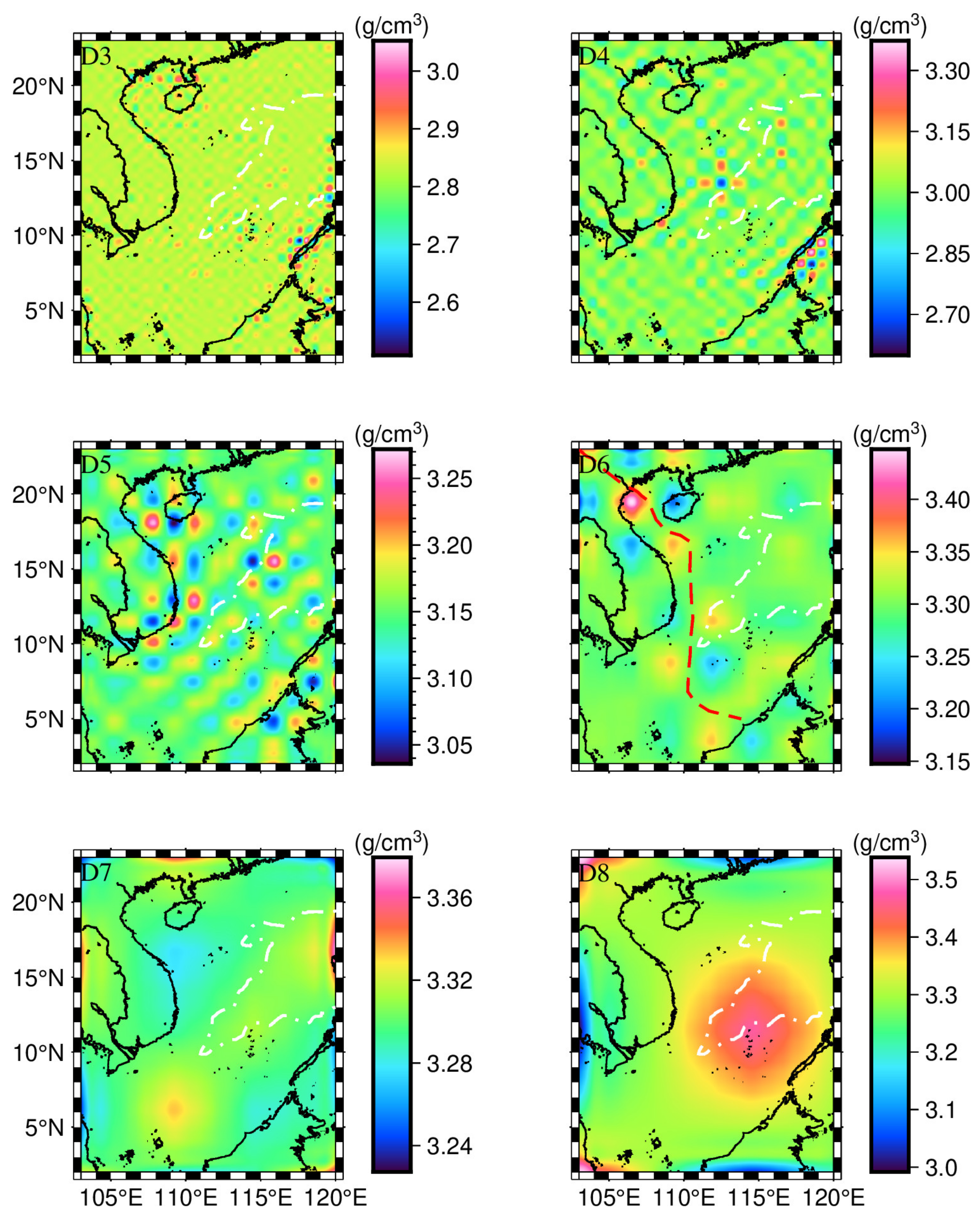
3.3. Stratified Density Inversion Results

Based on the field source depths that correspond to different orders of wavelet details, the structure of the SCS’s crust and upper mantle was stratified, and the thickness of each layer is presented in Table 1. Each layer of the structure was subsequently gridded and modeled using tesseroid bodies, with latitude and longitude spacings of 0.5°. After modeling, the density anomaly distribution for each layer was calculated using Equation (5). Furthermore, based on the CRUST 1.0 model, the average density of the different layers in the study area was calculated. For instance, D3 corresponds to the middle crust, and its average density is 2.83. D4 corresponds to the lower crust, and its average density is 3.01. D5 corresponds to the junction between the lower crust and the upper mantle, and the average density is taken as the average of the two, at 3.15. D6, D7, and D8 correspond to the upper mantle, and the average density is taken as 3.30. Density anomalies were added to the average density values for each layer, and the resulting density distribution for the different layers is shown in Figure 5.
Due to the low overall density variation observed in D1 and D2, along with the presence of noise in some areas, we have decided not to present the results for these layers. As shown in Figure 5, the density distribution for D3 spans depths ranging from 11.6 km to 17.4 km, with density values ranging from 2.51 g/cm3 to 3.04 g/cm3. Three regions exhibit the most significant density variation, with two located on either side of the PL, one at the BBWB, and the last at the junction of the SLS and CBS. Liu et al. [38] suggested that the extinct trench is located southeast of the present Palawan Trough, and we concur with this view. We speculate that the high-density material on either side of the PL is likely a tectonic component of the proto South China Sea. The BBWB is located at the junction of three large tectonic plates [41]. Previous research by Tapponnier et al. [42] attributed its extensional driving mechanism to extrusion caused by the collision between Indochina and Asia, while Yan et al. [43] attributed it to impact uplift of the Hainan mantle’s thermal column. Therefore, we suggest that the density anomaly observed in this region is highly correlated with tectonic evolution, and the material component may be evolutionary secondary material. D4 presents the density distribution at depths ranging from 17.4 km to 23.8 km in the SCS, with density values varying from 2.63 g/cm3 to 3.36 g/cm3. The main high-density areas are located in the northwestern part of the SLS. By combining the density changes on both sides of the PL observed in D3 and D4, we can observe a clear trend where high-density material disappears from the northwest to the southeast, indicating a potential sign of subduction. D5 shows the density distribution in the SCS from depths of 23.8 km to 42.4 km, with density values ranging from 3.04 g/cm3 to 3.27 g/cm3. The high-density anomalies observed in this layer almost cover the study area, suggesting that this region is likely located at the Moho surface, where tectonic movements are highly active. D6 presents the density distribution from depths of 42.4 km to 71.2 km in the SCS, with density values ranging from 3.14 g/cm3 to 3.44 g/cm3. An apparent high-density body occurs in the RRF’s vicinity, centered at 106.5°E and 19.5°N in longitude and latitude, respectively, with a diameter range of nearly 220 km. No previous studies have mentioned this high-density body, and its composition needs to be confirmed by subsequent studies. However, it is certain that there is some correlation with the complex tectonic evolution of the RRF. D7 presents the density distribution from depths of 71.2 km to 106.8 km in the SCS, with density values ranging from 3.23 g/cm3 to 3.38 g/cm3. The density distribution in this layer is relatively flat, indicating that the tectonic composition here is relatively homogeneous. We speculate that the main component in this region is primary mantle material. D8 presents the density distribution from depths of 106.8 km to 128.8 km in the SCS, with density values ranging from 2.99 g/cm3 to 3.53 g/cm3. Among these, we identified a very large-range high-density body for the first time, spanning a longitude range from 110°E to 118°E and a latitude range from 7°N to 16°N. The high-density body has a value only 0.1 g/cm3 higher than the surrounding area, which we believe is the result of long-term tectonic evolution weakening its prominent features. However, the outline boundaries are still distinct.
In summary, Figure 5 illustrates the density structure of the SCS’s crust and upper mantle. Evidently, the density distribution of D5 shows drastic variations due to its location near Moho. The density distribution at other depths is generally smooth, and although there are local variations, they still indicate a relatively stable structure. In addition, the density distribution of D3 and D4 provides new evidence for subduction near the PL. The density distribution of D6 and D8 demonstrates the location and morphology of the two high-density bodies, the possible causes of which are described later in the Discussion section.

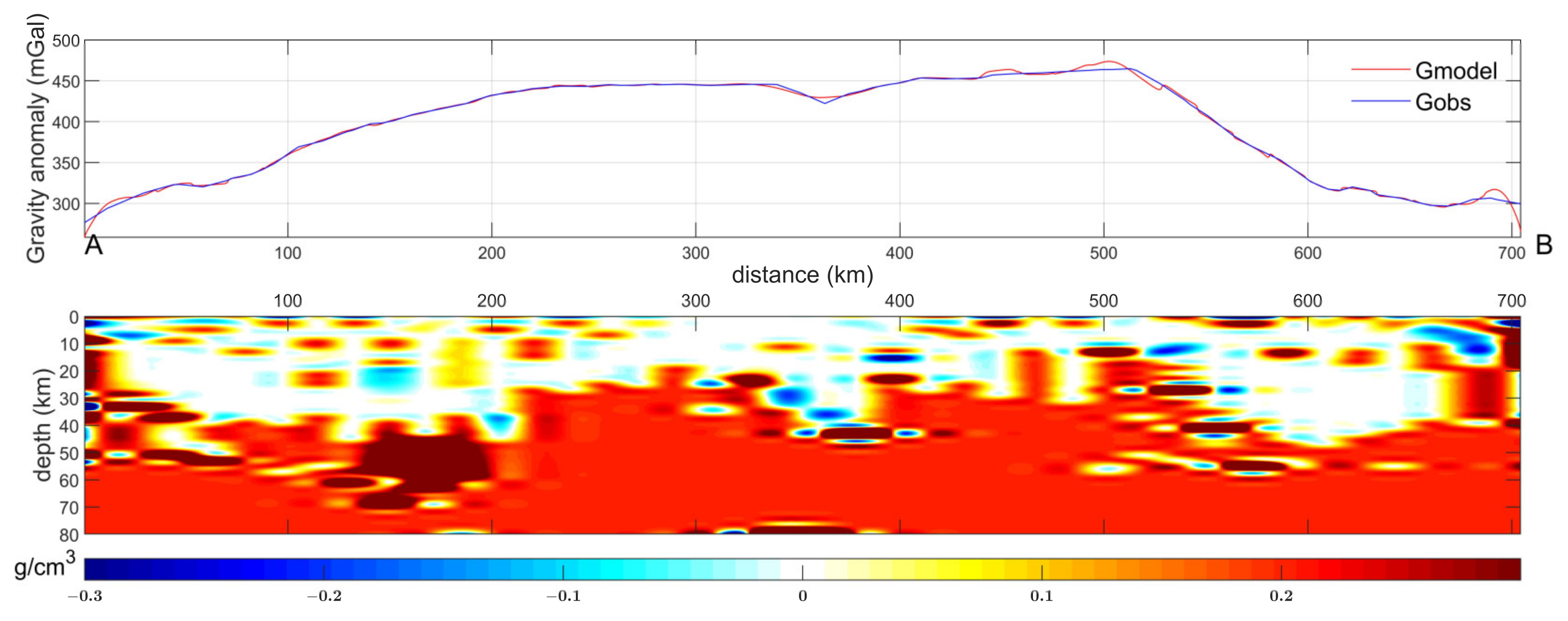
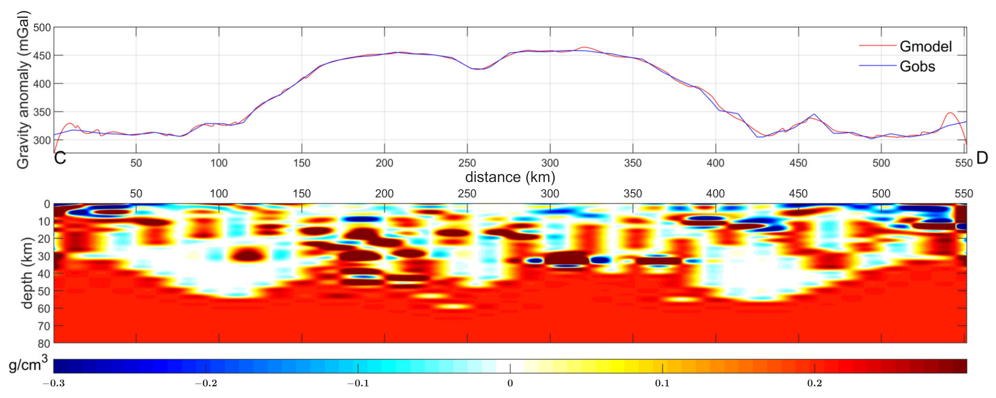
3.4. Profile Density

To more clearly demonstrate the density structure within the SCS, we selected two profiles A–B and C–D (as shown in Figure 2b), extracted the corresponding Bouguer gravity anomalies, and calculated the density distribution of the profiles using the compact gravity inversion method [44] (synthetic tests of this method have been performed previously [45]). Both profiles cross the SCSB, where the coordinates of point A are (113°E, 16°N), those of point B are (117°E, 11°N), those of point C are (112°E, 14°N), and those of point D are (115°E, 10°N). First, we modeled the subsurface structure of the profile with a 40 × 40 rectangular module and inverted the depth up to 80 km. Based on this, we iteratively inverted the density anomaly distribution of the profile, as shown in the lower subplots of Figure 6 and Figure 7. Finally, the gravity anomaly (Gmodel) obtained from the forward modeling was compared with the initial gravity anomaly (Gobs) to verify the reliability of the inversion results, as shown in the upper square plots in Figure 6 and Figure 7. From the upper subplots of Figure 6 and Figure 7, we can see that both Gmodel and Gobs are in good agreement, and the RMS values of the two are 3.2395 mGal and 4.6419 mGal respectively, proving that the inversion results are reliable.
The results in Figure 6 and Figure 7 show a clear high-density distribution in the area 200–550 km from Point A and 25–45 km in depth, and in the area 150–380 km from Point C and 10–50 km in depth. Combined with the SCS Moho topography results of Li et al. [46], we suggest that the main component of the high-density area is mantle material from the upper uplift. Previously, Hung et al. [47] had suggested, based on wave velocity results, that the crust is thinner near the extinct ridge and thicker away from the extinct ridge, which is consistent with the results shown in Figure 6 and Figure 7. It is noteworthy that the area in the range 330–380 km from point A, at a depth of 25–45, and the area 230–270 km from point C, at a depth of 25–45 km, correspond to the spreading ridge of the SCSB, with a retreat in density values compared to its sides, which also indicates that the spreading ridge is tectonically different from its sides. As to the cause of this phenomenon, we believe that there is a lack of magmatic power or the presence of deep tectonic faults. In addition, the area 650–700 km from point A and the area 500–550 km from point C correspond to the LYB, which has a phenomenon in its shallow part (within 20 km depth) where a high-density U-shaped body wraps around a low-density block, which is presumed to be a hydrocarbon storage area.

4. Discussion

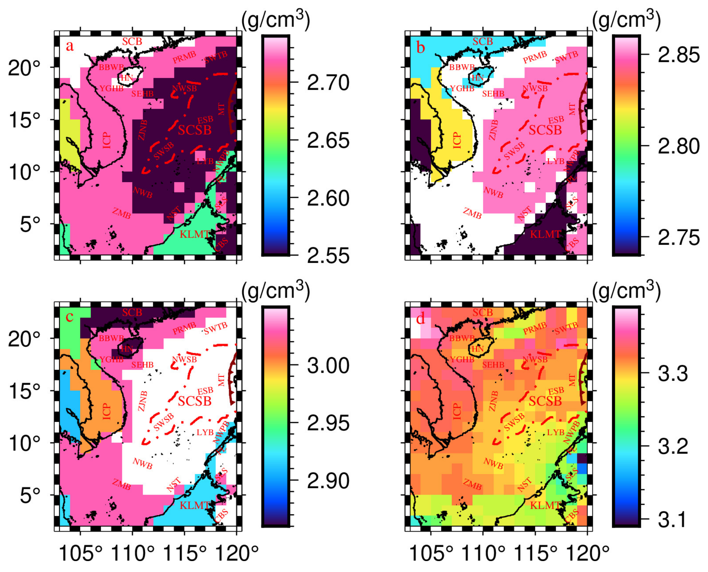
4.1. Internal Density Distribution in the SCS

To verify the accuracy of the stratified density inversion results (Figure 5), we selected the representative CRUST1.0 model (Figure 8) for comparison. The four subplots in Figure 8 represent the CRUST1.0 model’s density distribution at different layers. However, due to the spatial resolution of the image being 1° × 1°, only the overall variation can be observed, not the details. Figure 8b,c demonstrate clear density anomalies on both sides of the PL from middle to lower crustal depths, which is consistent with the findings in Figure 5(D3,D4). The difference is that the trend in density variation is not demonstrated in Figure 8 (the location of subduction in the proto South China Sea cannot be determined). Moreover, Figure 5(D3) displays a clear high-density anomaly near the BBWB, which largely matches the results in Figure 8b. A region in Figure 8c,d, to the right of the ZJNB, has a distinctly different density distribution, which is likely due to the spatial resolutions being different. Furthermore, because the mantle structure is not divided like the crust, the signal in Figure 8d is too concentrated to determine the density distribution of the mantle at different depths.
In summary, we believe that the stratified density inversion results show an improvement in detail. In particular, in the mantle region, the results in Figure 5 better demonstrate the density distribution of the mantle at different depths compared to CRUST 1.0.

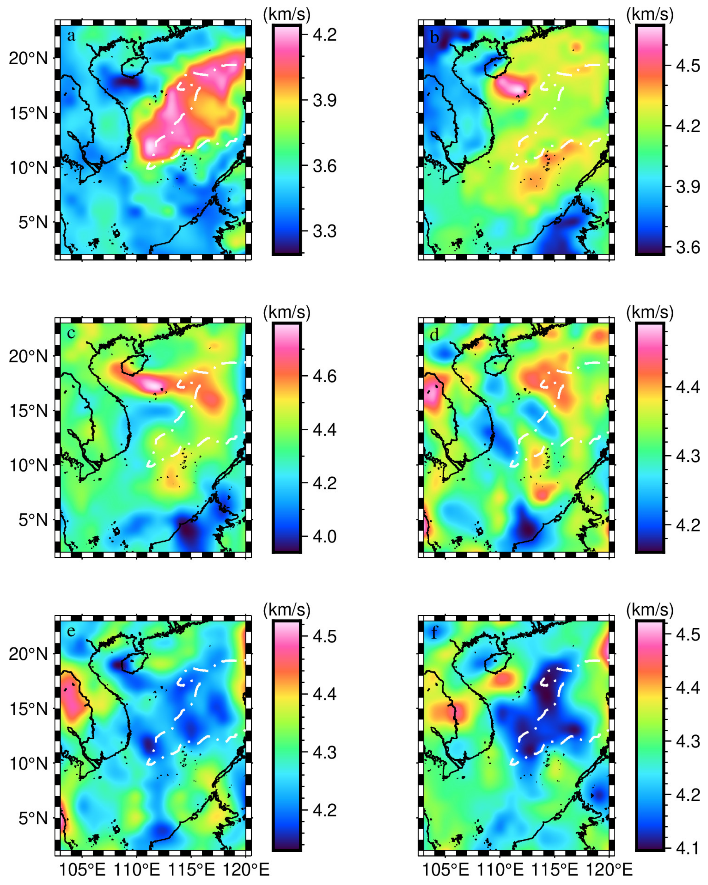
4.2. Comparison with the Velocity Model in the SCS

To enhance the discussion on the internal structure of the SCS, we refer to the findings of Chen et al. [48], as presented in Figure 9, and compare them with the stratified density results shown in Figure 5. The outcomes of Figure 9e,f reveal a distinctive low-velocity band ranging from 100 to 150 km within the SCSB. This region exhibits S-wave velocities between 4.1–4.15 km/s and is characterized by low velocities and high densities, as indicated by the results of Figure 5(D7,D8). Chen et al. [48] suggested that this location is situated in the asthenosphere and has partial mineral melting. Our results support this viewpoint, as we found that the asthenosphere typically exhibits low velocities and high densities, and that melting in this region may contribute to the insignificant density values of the high-density body near the NWSB in Figure 5.
Moreover, the outcomes of Figure 9c demonstrate a high-velocity band in the region near the YGHB at a depth of 45 km, where the S-wave velocities range from 4.55 to 4.6 km/s, which is in close proximity to the location of the first high-density body mentioned earlier. The results of Figure 9d show a high-velocity zone in northwest Thailand (approximately 114°E and 17°N) at a depth of 80 km, located on the western side of the YGHB basin, where the S-wave velocities range from 4.45 to 4.53 km/s. Figure 5(D6) also shows high-density material in the corresponding position, although the signal is weaker than that of the first high-density body. Therefore, we propose a bold hypothesis—the high-velocity zone in Figure 9c,d has essentially the same material composition. Furthermore, the first high-density body is mainly composed of material from the deep mantle of the Indochinese plate, and the primary reason for its formation is due to the collisional compression between the Indochinese plate and the Eurasian plate, resulting in the eastward upwelling of Indochinese deep mantle flow.
In summary, there is a close correlation between Figure 9 and Figure 5, such as in the location and morphology of the asthenosphere in the SCS. Furthermore, from the phenomenology of Figure 9, it can be concluded that the probable cause of the first high-density body in Figure 5 is the collisional compression of the Indochinese plate with the Eurasian plate.

4.3. Some New Discoveries

Figure 5 depicts the morphology of two high-density bodies within the SCS, which differ significantly in depth, extent, and shape. The first high-density body is located near the YGHB, with a depth range of 42.4 km to 71.2 km and a diameter close to 220 km. Sun et al. [7] previously suggested that the RRF exhibited leftward rotation until 5 Ma, followed by more pronounced rightward rotation after 5 Ma. Tapponnier et al. [42] proposed an extrusion model, suggesting that the Indochinese plate escaped towards the southeast, forming a strike–slip boundary. Therefore, we assume that the first high-density body may be a mantle flow formed by the collisional compression between the Indochinese and Eurasian plates, and that the high-density body is closely associated with the appearance of the RRF’s right-rotation feature.
The second high-density body is located near the NWSB, with a depth range of 106.8 km to 128.8 km and a circular planform. It is adjacent to the ICP towards the west and close to the PL towards the southeast. In our opinion, it may be part of the Paleo-Pacific remnant. As the second high-density body is located in a deeper mantle layer, and the density distribution is smoother under long-term tectonic evolution, its contribution to the gravity anomaly is not obvious in Figure 2b, which is why the high-density body inside the SCS has been neglected for a long time. Nevertheless, the second high-density body confirms, as a side effect, the distinctly different tectonics of the SCS in the north and south. Furthermore, it also explains, to some extent, the SCS’s evolutionary process.
Previously, there has been controversy regarding the extension model of the RRF. Hao et al. [49] suggested that the RRF extends southeastward to the SCS. Yao et al. [50] suggested that the RRF right-rotates northeastward through the SEHB and connects to the Xisha Trough. Sun et al. [51] suggested that the East Vietnam Fault is an extension of the RRF’s right-rotation based on simulation experiments. In the previous section, we proposed that there is a connection between the first high-density body and the RRF’s right-rotation. Therefore, we can assume that the density distribution in Figure 5(D6) is highly correlated with the extension of the RRF, and that there are significant differences in the structure on either side of the extension (i.e., large density differences).
Ludwig et al. [6] suggested that there is shear in the western part of the SCS, while Ben-Avraham et al. [3] and Hilde et al. [4] suggested that there is a transform fracture zone in eastern Vietnam. Combined with the outcomes of Figure 5, we speculate that the eastern Vietnam fracture is RRF extension, and we use the red dashed line to depict the RRF’s extension (general orientation, details to be studied), as shown in Figure 5. The red dashed line passes through the YGHB, SEHB, ZJNB, and ZMB, and ends at the KLMB.

5. Conclusions

In this paper, wavelet multiscale analysis was used to study the SCS and to isolate the Bouguer gravity anomaly signal at different depths, on the basis of which the fine density structure within the SCS was obtained. The separated Bouguer gravity anomaly signals and the corresponding power spectrum outcomes demonstrate that the Bouguer gravity anomaly signals at different field source depths have unique evolutionary characteristics. The stratified density outcomes reveal the existence of two high-density bodies with different depths and morphologies inside the SCS. Among them, one high-density body may have some connection to the evolution of the RRF, while the other high-density body is located at deeper depths, and we speculate that it may be part of the Paleo-Pacific remnant in the SCS. Additionally, we identified trends in proto South China Sea’s subduction and determined the geographical location of the subduction zone.

Author Contributions

Conceptualization, C.X. (Chuang Xu); methodology, H.Y. and C.X. (Chuang Xu); software, H.Y.; validation, H.Y. and H.C.; formal analysis, C.X. (Congcong Xing); investigation, Y.C. and G.W.; data curation, H.Z. and H.Y.; writing—original draft preparation, H.Y. and C.X. (Chuang Xu); writing—review and editing, C.X. (Chuang Xu) and P.Q.; visualization, M.X. and H.W.; supervision, C.X. (Chuang Xu); project administration, C.X. (Chuang Xu); funding acquisition, P.Q. All authors have read and agreed to the published version of the manuscript.

Funding

This research was funded by the National Natural Science Foundation of China (Grant nos. 42104136, 41974014, 42274004), Science and Technology Projects in Guangzhou (Grant no. 202201011216), the China Geological Survey (Grant no. DD20230649), and the Natural Science Foundation of Guangdong Province, China (Grant no. 2022A1515010396).

Data Availability Statement

The original contributions presented in this study are included in the article; further inquiries can be directed to the corresponding author.

Conflicts of Interest

The authors declare no conflict of interest.

References

  1. Ren, J.Y.; Lei, C. Tectonic stratigraphic framework of Yinggehai-Qiongdongnan Basins and its implication for tectonic province division in South China Sea. Chin. J. Geophys. 2011, 54, 3303–3314. [Google Scholar] [CrossRef]
  2. Zhao, C.Y.; Song, H.B.; Yang, Z.W.; Song, Y.; Tian, L.H. Tectonic and thermal evolution modeling for the marginal basins of the southern South China Sea. Chin. J. Geophys. 2014, 57, 1543–1553. [Google Scholar]
  3. Ben-Avraham, Z.; Emery, K.O. Structural framework of Sunda shelf. AAPG Bull. 1973, 57, 2323–2366. [Google Scholar]
  4. Hilde, T.W.C.; Uyeda, S.; Kroenke, L. Evolution of the western Pacific and its margin. Tectonophysics 1977, 38, 145–165. [Google Scholar] [CrossRef]
  5. Li, T.L.; Shi, H.Y.; Guo, Z.H.; Zhang, G.C.; Zhang, R.Z.; Chen, H.B. Research on deep structure of the South China Sea based on satellite gravity and magnetic data. Chin. J. Geophys. 2018, 61, 4216–4230. [Google Scholar]
  6. Ludwig, W.J.; Kumar, N.; Houtz, R.E. Profiler-sonobuoy measurements in the South China Sea basin. J. Geophys. Res. Solid Earth 1979, 84, 3505–3518. [Google Scholar] [CrossRef]
  7. Sun, Z.; Zhou, D.; Zhong, Z.; Zeng, Z.; Wu, S. Experimental evidence for the dynamics of the formation of the Yinggehai basin, NW South China Sea. Tectonophysics 2003, 372, 41–58. [Google Scholar] [CrossRef]
  8. Wu, Z.L.; Li, J.B.; Ruan, A.G.; Lou, H.; Ding, W.W.; Niu, X.W.; Li, X.B. Crustal structure of the northwestern sub-basin, South China Sea: Results from a wide-angle seismic experiment. Sci. China Earth Sci. 2012, 55, 159–172. [Google Scholar] [CrossRef]
  9. Ruan, A.; Wei, X.; Niu, X.; Zhang, J.; Dong, C.; Wu, Z.; Wang, X. Crustal structure and fracture zone in the Central Basin of the South China Sea from wide angle seismic experiments using OBS. Tectonophysics 2016, 688, 1–10. [Google Scholar] [CrossRef] [Green Version]
  10. Braitenberg, C.; Wienecke, S.; Wang, Y. Basement structures from satellite-derived gravity field: South China Sea ridge. J. Geophys. Res. Solid Earth 2006, 111, B05407. [Google Scholar] [CrossRef]
  11. Hao, T.Y.; Huang, S.; Xu, Y.; Li, Z.W.; Xu, Y.; Lei, S.M.; Yang, J.Y. Comprehensive geophysical research on the deep structure of Northeastern South China Sea. Chin. J. Geophys. 2008, 51, 1168–1180. [Google Scholar] [CrossRef]
  12. Guan, D.; Ke, X.; Wang, Y. Basement structures of East and South China Seas and adjacent regions from gravity inversion. J. Asian Earth Sci. 2016, 117, 242–255. [Google Scholar] [CrossRef]
  13. Gao, J.; Wu, S.; McIntosh, K.; Mi, L.; Liu, Z.; Spence, G. Crustal structure and extension mode in the northwestern margin of the South China Sea. Geochem. Geophys. Geosystems 2016, 17, 2143–2167. [Google Scholar] [CrossRef] [Green Version]
  14. Wu, Z.C.; Gao, J.Y.; Ding, W.W.; Shen, Z.Y.; Zhang, T.; Yang, C.G. The Moho depth of the South China Sea basin from three-dimensional gravity inversion with constraint points and its characteristics. Chin. J. Geophys. 2017, 60, 2599–2613. [Google Scholar]
  15. Sun, Z.; Ouyang, M.; Guan, B. Bathymetry predicting using the altimetry gravity anomalies in South China Sea. Geod. Geodyn. 2018, 9, 156–161. [Google Scholar] [CrossRef]
  16. Luo, X.G.; Wang, W.Y.; Zhang, G.C.; Zhao, Z.G.; Liu, J.L.; Xie, X.J.; Qiu, Z.Y.; Feng, X.L.; Ji, X.L.; Wang, D.D. Study on distribution features of faults based on gravity data in the South China Sea and its adjacent areas. Chin. J. Geophys. 2018, 61, 4255–4268. [Google Scholar]
  17. Zhang, J.; Yang, G.; Tan, H.; Wu, G.; Wang, J. Mapping the Moho depth and ocean-continent transition in the South China Sea using gravity inversion. J. Asian Earth Sci. 2021, 218, 104864. [Google Scholar] [CrossRef]
  18. Ji, F.; Li, F.; Zhang, Q.; Gao, J.Y.; Hao, W.F.; Li, Y.D.; Guan, Q.S.; Lin, X. Crustal density structure of the Antarctic continent from constrained 3-D gravity inversion. Chin. J. Geophys. 2019, 62, 849–863. [Google Scholar]
  19. Feng, J.; Meng, X.H.; Chen, Z.X.; Shi, L.; Wu, Y.; Fan, Z.J. The investigation and application of three-dimensional density interface. Chin. J. Geophys. 2014, 57, 287–294. [Google Scholar]
  20. Bi, B.T.; Hu, X.Y.; Li, L.Q.; Zhang, H.L.; Liu, S.; Cai, J.C. Multi-scale analysis to the gravity field of the northeastern Tibetan plateau and its geodynamic implications. Chin. J. Geophys. 2016, 59, 543–555. [Google Scholar]
  21. Xu, C.; Wang, H.; Luo, Z.; Liu, H.; Liu, X. Insight into urban faults by wavelet multiscale analysis and modeling of gravity data in Shenzhen, China. J. Earth Sci. 2018, 29, 1340–1348. [Google Scholar] [CrossRef]
  22. Hirt, C.; Rexer, M. Earth2014: 1 arc-min shape, topography, bedrock and ice-sheet models–Available as gridded data and degree-10,800 spherical harmonics. Int. J. Appl. Earth Obs. Geoinf. 2015, 39, 103–112. [Google Scholar] [CrossRef] [Green Version]
  23. Zingerle, P.; Pail, R.; Gruber, T.; Oikonomidou, X. The combined global gravity field model XGM2019e. J. Geod. 2020, 94, 66. [Google Scholar] [CrossRef]
  24. Straume, E.O.; Gaina, C.; Medvedev, S.; Gohl, K.; Whittaker, J.M.; Abdul Fattah, R.; Doornenbal, J.C.; Hopper, J.R. GlobSed: Updated total sediment thickness in the world’s oceans. Geochem. Geophys. Geosyst. 2019, 20, 1756–1772. [Google Scholar] [CrossRef]
  25. Laske, G.; Masters, G.; Ma, Z.; Pasyanos, M. Update on CRUST1. 0—A 1-degree global model of Earth’s crust. In Geophysical Research Abstracts; EGU General Assembly: Vienna, Austria, 2013; Volume 15, p. 2658. [Google Scholar]
  26. Mallat, S.G. A theory for multiresolution signal decomposition: The wavelet representation. IEEE Trans. Pattern Anal. Mach. Intell. 1989, 11, 674–693. [Google Scholar] [CrossRef] [Green Version]
  27. Spector, A.; Grant, F.S. Statistical models for interpreting aeromagnetic data. Geophysics 1970, 35, 293–302. [Google Scholar] [CrossRef]
  28. Heck, B.; Seitz, K. A comparison of the tesseroid, prism and point-mass approaches for mass reductions in gravity field modelling. J. Geod. 2007, 81, 121–136. [Google Scholar] [CrossRef]
  29. Tikhonov, A.N.; Arsenin, V.Y. Solotion of Ill-Posed Problems; John Wiley and Sons: Hoboken, NJ, USA, 1977. [Google Scholar]
  30. Hansen, P.C.; O’Leary, D.P. The use of the L-curve in the regularization of discrete ill-posed problems. SIAM J. Sci. Comput. 1993, 14, 1487–1503. [Google Scholar] [CrossRef]
  31. Parker, R.L. The rapid calculation of potential anomalies. Geophys. J. Int. 1973, 31, 447–455. [Google Scholar] [CrossRef] [Green Version]
  32. Lu, B.L.; Wang, W.Y.; Zhao, Z.G.; Feng, X.L.; Zhang, G.C.; Luo, X.G.; Yao, P.; Ji, X.L. Characteristics of deep structure in the South China Sea and geological implications: Insights from gravity and magnetic inversion. Chin. J. Geophys. 2018, 61, 4231–4241. [Google Scholar]
  33. Xie, X.N.; Ren, J.Y.; Wang, Z.F.; Li, X.S.; Lei, C. Difference of tectonic evolution of continental marginal basins of South China Sea and relationship with SCS spreading. Earth Sci. Front. 2015, 22, 77–87. [Google Scholar]
  34. Xu, C.; Liu, Z.; Luo, Z.; Wu, Y.; Wang, H. Moho topography of the Tibetan Plateau using multiscale gravity analysis and its tectonic implications. J. Asian Earth Sci. 2017, 138, 378–386. [Google Scholar] [CrossRef]
  35. Rangin, C. The Sulu Sea, a back-arc basin setting within a Neogene collision zone. Tectonophysics 1989, 161, 119–141. [Google Scholar] [CrossRef]
  36. Rangin, C.; Silver, E.A. Neogene tectonic evolution of the Celebes-Sulu basins: New insights from Leg 124 drilling. Proc. Ocean Drill. Program Sci. Results 1991, 124, 51–63. [Google Scholar]
  37. Wang, S.; Zhang, G. Geochemical constraints on mantle source nature and recycling of subducted sediments in the Sulu Sea. Geosyst. Geoenviron. 2022, 1, 100005. [Google Scholar] [CrossRef]
  38. Liu, W.N.; Li, C.F.; Li, J.; Fairhead, D.; Zhou, Z. Deep structures of the Palawan and Sulu Sea and their implications for opening of the South China Sea. Mar. Pet. Geol. 2014, 58, 721–735. [Google Scholar] [CrossRef]
  39. Zhu, M.; Graham, S.; McHargue, T. The red river fault zone in the Yinggehai Basin, South China Sea. Tectonophysics 2009, 476, 397–417. [Google Scholar] [CrossRef]
  40. Mazur, S.; Green, C.; Stewart, M.G.; Whittaker, J.M.; Williams, S.; Bouatmani, R. Displacement along the Red River Fault constrained by extension estimates and plate reconstructions. Tectonics 2012, 31, TC5008. [Google Scholar] [CrossRef]
  41. Gong, Y.; Pease, V.; Wang, H.; Gan, H.; Liu, E.; Ma, Q.; Zhao, S.; He, J. Insights into evolution of a rift basin: Provenance of the middle Eocene-lower Oligocene strata of the Beibuwan Basin, South China Sea from detrital zircon. Sediment. Geol. 2021, 419, 105908. [Google Scholar] [CrossRef]
  42. Tapponnier, P.; Peltzer, G.; Le Dain, A.Y.; Armijo, R.; Cobbold, P. Propagating extrusion tectonics in Asia: New insights from simple experiments with plasticine. Geology 1982, 10, 611–616. [Google Scholar] [CrossRef]
  43. Yan, Q.; Shi, X.; Castillo, P.R. The late Mesozoic–Cenozoic tectonic evolution of the South China Sea: A petrologic perspective. J. Asian Earth Sci. 2014, 85, 178–201. [Google Scholar] [CrossRef] [Green Version]
  44. Last, B.J.; Kubik, K. Compact gravity inversion. Geophysics 1983, 48, 713–721. [Google Scholar] [CrossRef]
  45. Yu, H.; Xu, C.; Wu, Y.; Li, J.; Jian, G.; Xu, M. Fine structure of the lunar crust and upper mantle in the mare serenitatis derived from gravity multi-scale analysis. Front. Astron. Space Sci. 2023, 10, 1109714. [Google Scholar] [CrossRef]
  46. Li, J.; Xu, C.; Chen, H. An improved method to Moho depth recovery from gravity disturbance and its application in the South China Sea. J. Geophys. Res. Solid Earth 2022, 127, e2022JB024536. [Google Scholar] [CrossRef]
  47. Hung, T.D.; Yang, T.; Le, B.M.; Yu, Y.; Xue, M.; Liu, B.; Liu, C.; Wang, J.; Pan, M.; Huong, P.T.; et al. Crustal structure across the extinct mid-ocean ridge in South China sea from OBS receiver functions: Insights into the spreading rate and magma supply prior to the Ridge cessation. Geophys. Res. Lett. 2021, 48, e2020GL089755. [Google Scholar] [CrossRef]
  48. Chen, H.; Li, Z.; Luo, Z.; Ojo, A.O.; Xie, J.; Bao, F.; Wang, L.; Tu, G. Crust and upper mantle structure of the South China Sea and adjacent areas from the joint inversion of ambient noise and earthquake surface wave dispersions. Geochem. Geophys. Geosystems 2021, 22, e2020GC009356. [Google Scholar] [CrossRef]
  49. Hao, T.; Liu, J.; Song, H.; Xu, Y. Geophysical Evidences of Some Important Faults in South China and Adjacent Marginal Seas Region. Prog. Geophys. 2002, 17, 13–23. [Google Scholar]
  50. Yao, B.; Zeng, W.; Chen, Y.; Zhang, X.; Hayes, D.E.; Diebold, J.; Buhl, P.; Spangler, S. Xisha trough of South China Sea–An ancient suture. Mar. Geol. Quat. Geol. 1994, 14, 1–9. [Google Scholar]
  51. Sun, Z.; Zhong, Z.; Zhou, D.; Lin, X.; Wu, S. Deformation Mechanism of Red River Fault Zone during Cenozoic and Experimental Evidences related to Yinggehai Basin Formation. J. Trop. Oceanogr. 2003, 22, 1–9. [Google Scholar]
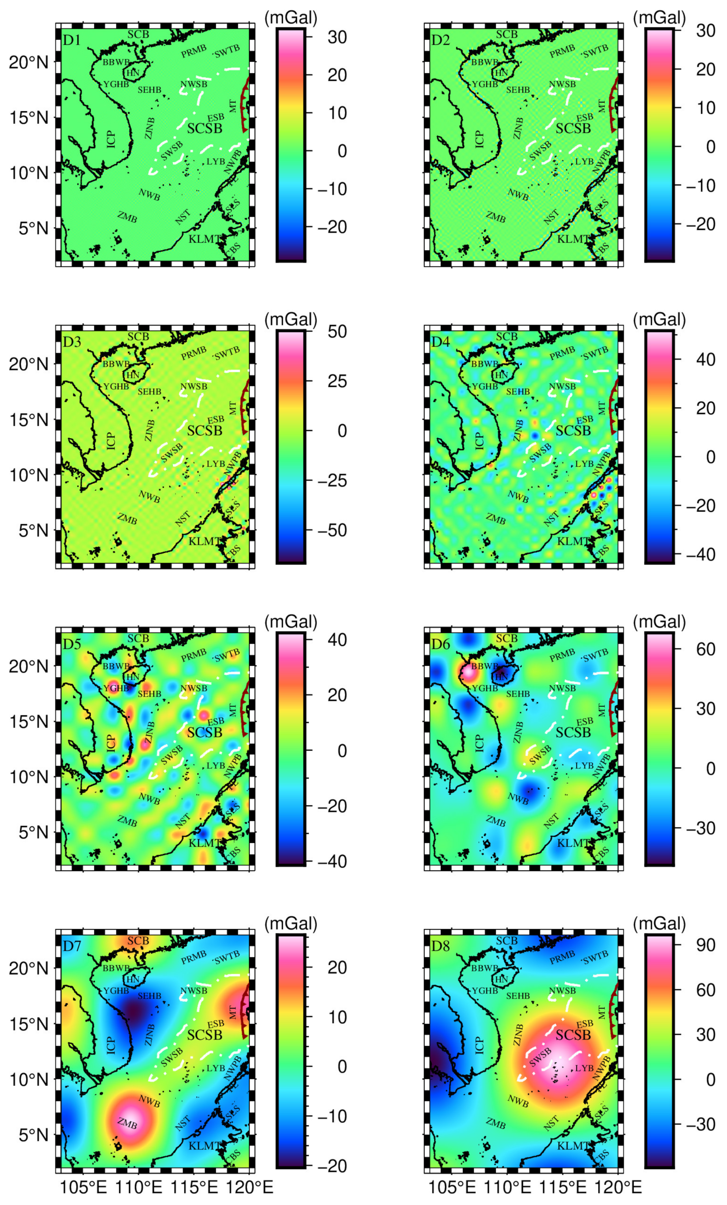
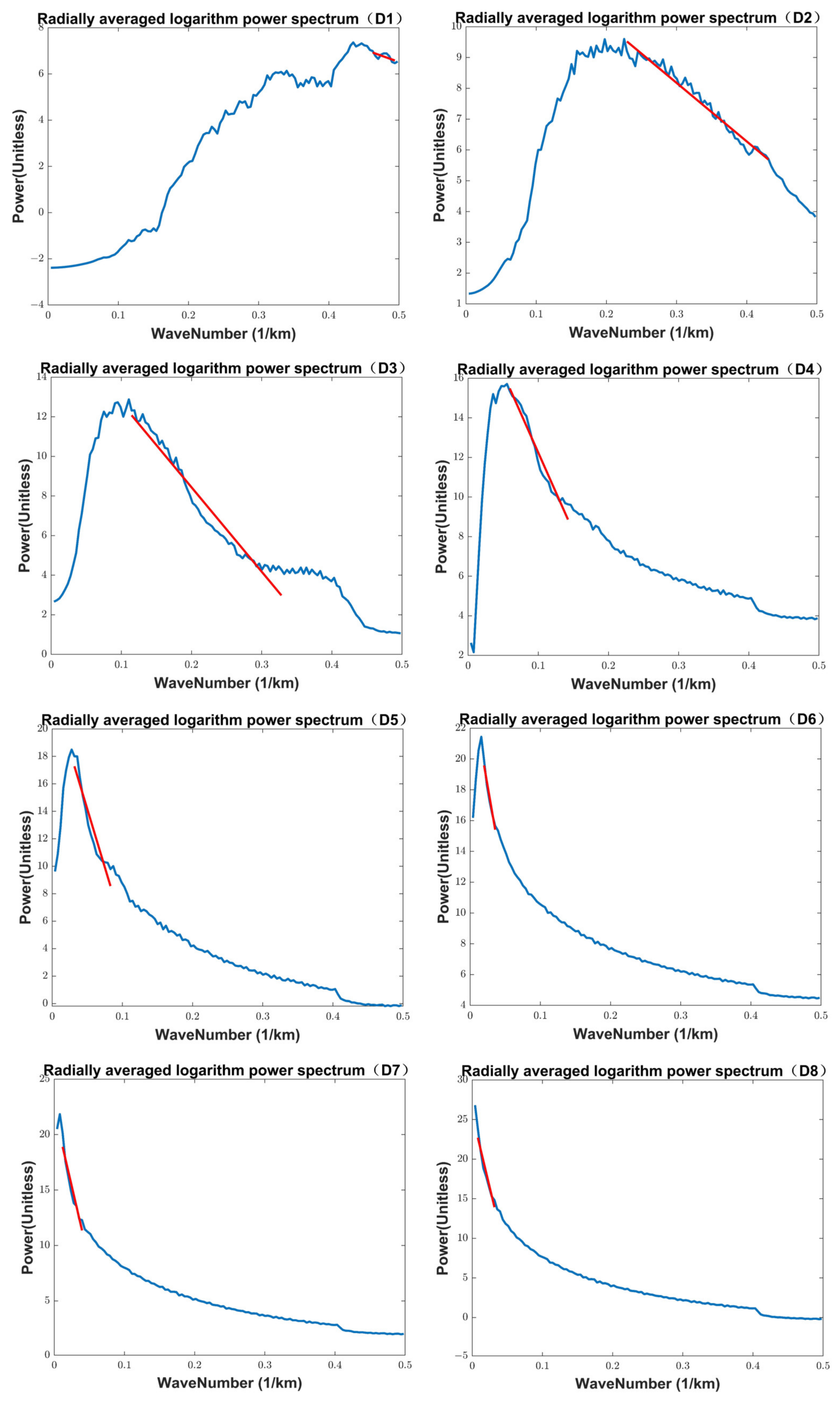
Figure 1. Topography of the SCS. SCB: South China Block, PRMB: Pear River Mouth Basin, SEHB: Southeast Hainan Basin, SWTB: Southwest Taiwan Basin, SCSB: South China Sea Basin, KLMT: Kalimantan Island, HN: Hainan Island, ICP: Indochina Peninsula, LYB: Liyue Basin, YGHB: Yinggehai Basin, PL: Palawan Island, NWSB: northwest sub-basin, SWSB: southwest sub-basin, ESB: east sub-basin, MT: Manila Trench, NST: Nansha Trough, ZMB: Zengmu Basin, ZJNB: Zhongjiannan Basin, NWPB: Northwest Palawan Basin, BBWB: Beibuwan Basin, NWB: Nanwei Basin, SLS: Sula Sea, CBS: Celebes Sea, RRF: Red River Fault, COT: Continental–oceanic transition. The light red lines represent the continent–ocean boundary (COB). The dark red lines with dark red triangles represent trenches.
Remotesensing 15 03274 g001
Figure 2. Free-air gravity anomaly (a) and Bouguer gravity anomaly (b) of the SCS.
Remotesensing 15 03274 g002
Figure 3. Decomposed Bouguer gravity anomalies D1–D8 in the SCS.
Remotesensing 15 03274 g003
Figure 4. Radial logarithm power spectrum of the decomposed gravity anomalies D1–D8 in the SCS.
Remotesensing 15 03274 g004
Figure 5. Stratified density inversion results.
Remotesensing 15 03274 g005
Figure 6. Profile density anomaly distribution of A–B in the SCS.
Remotesensing 15 03274 g006
Figure 7. Profile density anomaly distribution of C–D in the SCS.
Remotesensing 15 03274 g007
Figure 8. Density distribution in CRUST1.0: (a) Upper crust. (b) Middle crust. (c) Lower crust. (d) Mantle.
Remotesensing 15 03274 g008
Figure 9. Three-dimensional S-wave velocity model in the SCS: (a) 15 km. (b) 30 km. (c) 45 km. (d) 80 km. (e) 100 km. (f) 150 km [48].
Remotesensing 15 03274 g009
Table 1. The average depth and thickness of each layer.
LayerRange of Depth (km)Average Depth (km)Thickness (km)
D10.0~2.01.02.0
D22.0~11.66.89.6
D311.6~17.414.55.8
D417.4~23.820.66.4
D523.8~42.433.118.6
D642.4~71.256.828.8
D771.2~106.889.035.6
D8106.8~128.8117.822.0
Disclaimer/Publisher’s Note: The statements, opinions and data contained in all publications are solely those of the individual author(s) and contributor(s) and not of MDPI and/or the editor(s). MDPI and/or the editor(s) disclaim responsibility for any injury to people or property resulting from any ideas, methods, instructions or products referred to in the content.

