
Sea Clutter Amplitude Prediction via an Attention-Enhanced Seq2Seq Network

1
Electronic Information School, Wuhan University, Wuhan 430072, China
2
Air Force Early Warning Academy, Wuhan 430019, China
3
School of Electronic Engineering, Naval University of Engineering, Wuhan 430033, China
*
Author to whom correspondence should be addressed.
Remote Sens. 2023, 15(13), 3234; https://doi.org/10.3390/rs15133234
Submission received: 31 March 2023
/
Revised: 8 June 2023
/
Accepted: 20 June 2023
/
Published: 22 June 2023
(This article belongs to the Special Issue Multi-Dimensional Radar Sensing: Systems, Algorithms, and Applications)
Abstract
:Sea clutter is a kind of ubiquitous interference in sea-detecting radars, which will definitely influence target detection. An accurate sea clutter prediction method is supposed to be beneficial while existing prediction methods are based on the one-step-ahead prediction. In this paper, a sea clutter prediction network (SCPNet) is proposed to achieve the k-step-ahead prediction based on the characteristics of sea clutter. The SCPNet takes a sequence-to-sequence (Seq2Seq) structure as the backbone, and a simple self-attention module is employed to enhance the ability of adaptive feature selections. The SCPNet takes the normalized amplitudes of sea clutter as inputs and is capable of predicting an output sequence with a length of k; the phase space reconstruction theory is also used to find the optimized input length of the sea clutter sequence. Results with the sea-detecting radar data-sharing program (SDRDSP) database show the mean square error of the proposed method is 1.48 × 10⁻⁵ and 8.76 × 10⁻³ in the one-step-ahead prediction and the eight-step-ahead prediction, respectively. Compared with four existing methods, the proposed method achieves the best prediction performance.

1. Introduction
Real-time and accurate marine surveillance plays a significant role in both military and civil fields, such as early warning and marine rescue [1]. Radar, which served as a full-weather and full-time sensor, is a ubiquitous solution to provide reliable range and Doppler resolutions. However, back-scattering echoes received by radar systems contain not only targets under test but also echoes from the sea surface. These echoes from the sea surface, i.e., sea clutter, are supposed to interfere with the observation of targets of interest. Once the sea wave becomes sufficiently wild, it will introduce the probability of a false alarm, which is almost inevitable in many kinds of radar systems [2,3]. In addition, owing to its physical property, the Doppler spectrum of sea clutter is prone to being wide. The wide Doppler spectrum then tends to cover targets under test [4], especially those dim targets with a relatively low velocity. Thus, it is of significance to suppress sea clutter while preserving the information of targets of interest.
There are lots of classical clutter-suppression algorithms based on transform domain cancellation, such as the moving target indicator (MTI) method and root loop cancellation. Nevertheless, targets with a low velocity are likely to be suppressed along with sea clutter by the MTI method. In addition, the spectrum center of sea clutter will not always be consistent with the zero Doppler frequency due to the relative motion of the sea surface, which is prone to performance degradation of these cancellation methods [5]. In addition, subspace projection methods also provide solutions to suppress clutter, such as the singular-value decomposition method [6]. Based on the multiresolution analysis and reconstruction theory, a series of clutter-suppression approaches are proposed via many kinds of wavelet transforms [7]. Empirical mode decomposition is also introduced into the sea clutter-suppression method [8]. Although these suppression methods have improved the clutter-suppression ability, sea clutter has obvious nonlinear, non-Gaussian, and nonstationary characteristics [9], which may cause performance degradation.
Except for the typical suppression methods mentioned above, another viable way to achieve robust clutter suppression is to predict the amplitude of sea clutter by learning its natural inner rules. Then, a simple cancellation in the time domain between received echoes and extrapolated clutter sequences can be employed to highlight targets of interest. A large number of references focused on clutter characteristics are proposed. For the characteristic of amplitude distribution, the Rayleigh distribution is designed for radar systems with low resolutions. The log-normal distribution is proposed for sea clutter with large dynamic ranges. The Weibull distribution and the K distribution are also widely used in clutter models. Later, more and more elaborate models are proposed to describe sea clutter [10].
As for the change rule with the time of sea clutter, it has been viewed as a stochastic process for a long time. In 1990, Haykin and Leung calculated and analyzed the correlation dimension of sea clutter, which first indicates that sea clutter is basically a chaotic process [11]. Furthermore, they have proposed a chaotic signal-processing method and a small-target detection method based on the chaotic characteristic [12,13]. Fortunately, the chaotic process of sea clutter actually provides a theoretical basis for clutter prediction. Leung has proposed a memory-based predictor to achieve nonlinear clutter cancellation [14]. A multimodel prediction approach is designed for sea clutter modeling in [15], and different radial basis neural networks are utilized to predict the peak of sea clutter.
With the development of machine learning, the support vector machine (SVM) is employed to predict real-life sea clutter data [16]. A sea clutter sequence prediction method based on a general-regression neural network (GRNN) and the particle-swarm optimization algorithm is proposed in [17]. Results with one dataset from the IPIX database [18] verify the feasibility of sea clutter prediction by a regression model, and the mean square error (MSE) of the proposed method is about 0.4754. In [19], the Volterra filter is employed to predict sea clutter and then detect low-flying targets and results with one dataset of the IPIX database indicating the MSE is about 3.24 × 10⁻³. A weighted grey Markov model is constructed for quantitative prediction of sea clutter power in [20]. Results with measured data show the proposed model has better prediction accuracy.
Recently, modern neural networks (NNs) and deep learning (DL) have gained great popularity and improvement in lots of fields, such as computer vision and natural language processing. Hence, more and more researchers are making efforts to combine radar signal processing algorithms and DL-based methods [21,22,23]. As for the prediction of sea clutter, since the amplitude of sea clutter can be described as a sequence varying with time, the clutter prediction problem can be viewed as a sequence prediction problem in the natural language processing society. Recurrent neural networks (RNNs), equipped with hidden states, are capable of catching and preserving short-term information in sequences [24]. Nevertheless, plain RNNs are prone to the gradient exploding problem and the vanishing gradient problem.
Long short-term memory networks (LSTMs) are designed to deal with the above problems by introducing the gate mechanism [25]. LSTMs are consequently utilized to solve the clutter prediction problem. To obtain higher prediction accuracy at a farther distance, an LSTM model is proposed, and its hyperparameters are discussed in [26]. Simulations demonstrate that the optimized LSTM model has better prediction accuracy compared with the backpropagation network. Further, a clutter amplitude prediction system based on an LSTM is designed in [27]. Results from three real-life databases show that the mean MSE of the proposed system is lower than that of the artificial neural network (ANN) and radial basis function network.
Except for the LSTM structure, a deep neural network (DNN) is employed to predict sea clutter characteristics via marine environmental factors in [28]. Results verify that the DNN model can effectively predict important characteristics of sea clutter in the South China Sea. In [29], a gated feedback RNN (GF-RNN) is designed to predict sea clutter amplitude. Two measured databases, namely the IPIX database and a P-band database, are used to evaluate the prediction performance. Results show that the GF-RNN has better prediction ability than the SVM and ANN.
Although existing RNN-based methods have achieved high prediction accuracy or low MSE with several real-life databases, these methods all use one-step-ahead prediction to obtain corresponding results. That is, they usually predict only one amplitude value due to the one-step-ahead prediction, which may be inefficient and complex to get a required long prediction in practice. Thus, a k-step-ahead prediction is urgent for sea clutter prediction. However, existing plain RNN-based methods may be powerless to deal with a long output sequence.
Aiming at the above shortcoming of existing methods, a sea clutter prediction network, denoted as SCPNet is proposed in this paper to achieve the k-step-ahead prediction. The proposed SCPNet takes a sequence-to-sequence (Seq2Seq) structure as a backbone and is enhanced by a self-attention module. Hence, different from the existing methods based on one-step-ahead prediction, the purpose of this paper is to attempt to explore the prediction performance of the k-step-ahead prediction method. The difficulty and shortcomings are then analyzed and summarized through experiments with a real-life database. The main contributions of this paper are as follows:
- Different from mainstream methods based on the one-step-ahead prediction, the proposed SCPNet is capable of predicting a long output sequence in one prediction via the k-step-ahead prediction, which is more helpful in practice and can be easily transformed into the one-step-ahead prediction when needed;
- A Seq2Seq model is introduced to deal with the problem of variable-length output sequences. The Seq2Seq model is capable of encoding input sequences and then decoding them as prediction sequences. Furthermore, a self-attention module is integrated to boost the learning and representation ability;
- Although the IPIX database is a widely used benchmark, some physical parameters are relatively out-of-date owing to the limitations of the hardware. Instead, a newly released database [30], namely the sea-detecting radar data-sharing program (SDRDSP) database, is employed to assess the performance of each method.
The rest of this paper is organized as follows: Section 2 provides a problem formulation, the difference between one-step-ahead prediction and the k-step-ahead prediction, and an introduction to phase space reconstruction and the SDRDSP database. The details of the proposed method, the structure of the SCPNet, and the experiment setting are presented in Section 3. The results of the phase space reconstruction and comparisons of different prediction modes are given and analyzed in Section 4. The consistency analysis and the computational complexity are discussed in Section 5. Finally, the conclusions of this paper and future works are summarized in Section 6.
2. Materials
In this subsection, the sea clutter prediction problem is formulated to clarify the theoretical basis and contributions. Further, a brief introduction to the phase space reconstruction theory is provided. Some detailed physical parameters and experiment settings of the employed SDRDSP database are finally introduced.
2.1. Sea Clutter Properties and Problem Formulation
There are lots of research focused on the sea clutter model from different points of view, such as the amplitude distribution, the Doppler domain, and spatial and temporal correlations. The amplitude distribution is always used to describe the stochastic fluctuation of sea clutter through the probability density function (PDF). As mentioned in the introduction, some typical distribution models are employed to fit the amplitude distribution of actual sea clutter, including the Rayleigh distribution, the log-normal distribution, the Weibull distribution, and the K distribution. Furthermore, there are more and more elaborate models to describe actual sea clutter in recent years.
For echoes of sea clutter, the Bragg scatting returns are significant components, and they yield two distinct Doppler frequencies when the carrier frequency is lower than the L-band. When the carrier frequency is higher than the L-band, there is usually only one Bragg peak in the frequency spectrum [31]. These Doppler frequencies can be calculated as [32]
where is the carrier frequency, is the gravity acceleration, and is the speed of light. The analysis of temporal and spatial correlations can indicate a strong correlation in the range domain and the time domain, respectively. Mathematically, for a fully coherent radar overlooking a clutter-only ocean, the received sea clutter sequence with N sample points can be denoted as
Then, the temporal correlation coefficient and the spatial correlation coefficient are defined as [33]
where is the correlation function in the time domain and is the mathematical expectation. According to these properties, it is viable to learn inner features and predict the probable future fluctuation of sea clutter through NNs. Afterward, the extrapolated clutter sequence can be employed to detect an anomaly, especially the presence of a target by comparing it with the actual received echoes.
Since most existing NNs cannot process complex-value signals, the absolute value of the received clutter sequence then becomes an alternate, denoted as . Due to the complex nonlinear and chaotic characteristics of sea clutter, the absolute value sequence is usually normalized, which is also beneficial to training RNNs. Herein, a min-to-max normalization is employed as follows:
where and are the minimal value and the maximal value, respectively. Then according to Takens’ embedding theorem [34], the chaotic sequence can be reconstructed as:
where . and denote the delay time and embedding dimension, respectively [35]. is the i-th reconstructed sequence. Through the phase space reconstruction theory, a state transition function can be calculated as
Apparently, the nonlinear transition function is the key to predicting the next value. However, how to find the function is a rather challenging task. Thanks to the universal approximation theorem, a full-connection RNN with adequate sigmoid-class hidden neurons is capable of fitting any nonlinear dynamic systems [36]. Thus, can be obtained through data-driven training. Equation (4) then is rewritten as
where denotes a RNN and is the prediction value of the RNN. As for the training of the RNN, supervised learning is employed to obtain the optimized weights. For a given training sample , where denote the training sequence and denote the label sequence, the error of prediction is calculated via a loss function as follows
where is the loss function and is the learnable parameter in the RNN. Herein, the loss function is the MSE function that is widely used in the prediction problem. The MSE function is defined as
where is the length of the prediction sequence; and denote the i-th true value and i-th prediction value, respectively.
Next, our goal is to minimize the MSE between training samples and labels, and backpropagation through a time algorithm is used to train the RNN. However, it is hard to build a robust dependent relationship for a long range owing to the gradient exploding problem. So, a gradient clipping method is introduced during the training. Let denote the current gradient; then the gradient clipping performs the following steps:
where indicates a 2-norm and is a hyperparameter.
2.2. Phase Space Reconstruction
The length of an input clutter sequence is an important hyperparameter that, no doubt, will influence the prediction performance of RNNs. How to select the optimized length then becomes another difficulty. The length is manually selected by a series of experiments in lots of previous works, which, however, is a time-consuming job and cannot guarantee optimization. Thus, the phase space reconstruction theory is introduced in this paper to find the optimized length of the input sequence.
The received clutter sequence is actually a scalar that is more appropriate to analyze dynamic and chaotic characteristics in one-dimensional space. Thus, a phase space reconstruction is used to construct a higher dimensional space in the chaotic system for the clutter sequence, which can preserve the inner geometric properties of the original system. In addition, according to Takens’ embedding theorem, when an appropriate embedding dimension is selected, a phase space with the same meaning as the original system can be reconstructed by using the original time series, just as derived in Equation (3).
Under ideal conditions, the delay time and the embedding dimension can be stochastically determined for a noise-free sequence with infinite length. However, for the finite clutter sequence with lots of noise, it is of significance to calculate and precisely since inaccurate and are supposed to interfere with reconstruction performance and follow-up analysis. Once the optimized and are selected, the optimized input length is then selected. That is, the optimized length equals , just as indicated in Equation (4).
There are lots of algorithms to find the optimized , such as the autocorrelation algorithm and the mutual information algorithm. For a chaotic and nonlinear system, the mutual information algorithm is a better choice. Let and denote two discrete systems, and and are the information entropy of and , respectively. Then the mutual information is defined as
where is the conditional probability density (CPD). For each element in two systems, can be rewritten as
where is the joint probability density function. If we denote , that is, represents the sequence and represents the sequence with the delay time . Then, is a function with the delay time , denoted as . When , there is no correlation between and . The first minimal value of actually indicates the most unrelated relation between and , and the first minimal value consequently is the optimized delay time.
Once the delay time is selected, the Cao method [37] is employed to find the optimized . In the phase space with dimensions, each point vector is supposed to have the nearest point at a certain distance. When the dimension is , the distance will change and there will be the nearest point . Then, a variable is defined as
where denotes the Euclidean distance. Further, and are defined as
If does not change after is greater than a certain value, the optimized embedding dimension has been determined.
2.3. The One-Step-Ahead Prediction and the k-Step-Ahead Prediction
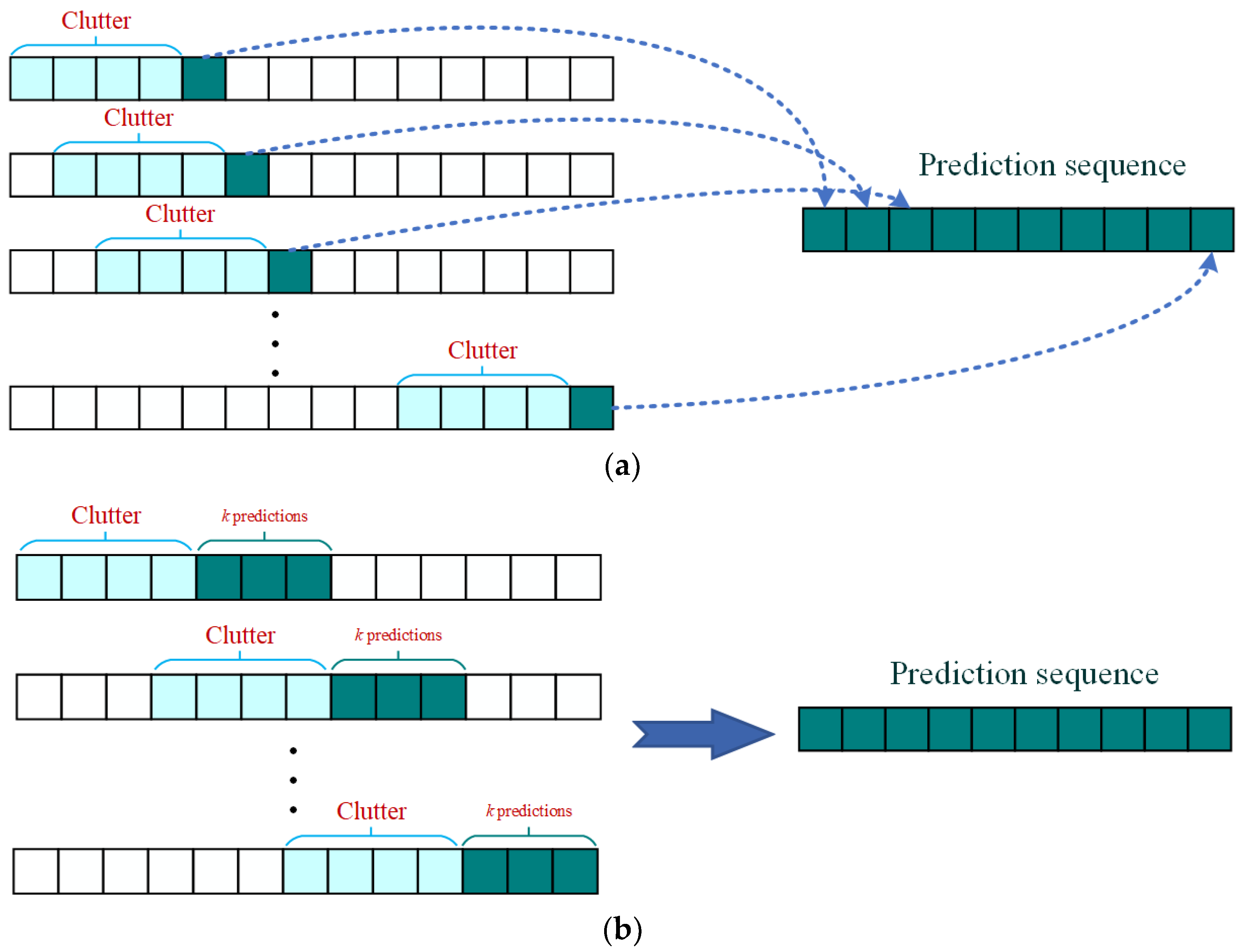
In the prediction problem, there are always two direct issues that remain to be dealt with, namely the length of the input sequence and the length of the output sequence in one prediction. Now that the former issue has been solved in the above subsection, it comes to the output length. Just as mentioned in the introduction part, existing methods almost depend on the one-step-ahead prediction, which means that they output only one value in one prediction. If a long prediction sequence is required, a recursive one-step-ahead prediction strategy is employed to achieve the prediction of a long sequence. When the length of an expected output sequence is , the one-step-ahead prediction should be recursively repeated times, just as shown in Figure 1a.
In Figure 1a, the boxes in each row represent a one-step-ahead prediction. The blue boxes mean the input sea clutter sequence in one prediction, and the dark blue box denotes the prediction value. After a series of predictions, a long prediction sequence is then obtained. In addition, a viable way to realize the k-step-ahead prediction via the one-step-ahead prediction is the recursive one-step-ahead prediction. That is, the current prediction value is supposed to be added to the next input sequence. Apparently, when the required length of the output sequence is relatively long, prediction errors of the recursive one-step-ahead prediction will be accumulated.
Different from the one-step-ahead prediction, a multiple-input multiple-output method is employed to achieve k-step-ahead prediction in this paper. Specifically, the length of the input sequence is the same as that of the one-step-ahead prediction, but it can output multiple values in one prediction, just as shown in Figure 1b. In one prediction, the k-step-ahead prediction directly outputs k values to arrange a prediction sequence. Apparently, the number of predictions for the k-step-ahead prediction is much lower than that of the one-step-ahead prediction.
2.4. The SDRDSP Database
In spite of the fact that the IPIX database has been a classical benchmark in sea clutter prediction and floating target detection, it has been nearly 30 years since the first issue of the IPIX database was proposed. Particularly, with the rapid development of advanced radar systems, some physical parameters of the IPIX database, such as the range resolution of 30 m, are relatively out-of-date and may not adequately evaluate modern signal-processing methods.
Learning from the success of the IPIX database and other open-access databases, the SDRDSP database [30] is released by the Naval Aviation University to promote research on clutter characteristics, sea clutter suppression, and target detection. The employed X-band radar is a solid-state power amplifier radar for coastal surveillance and navigation, which has the advantages of high resolution, high reliability, and a small distance blind area. The detailed physical parameters are listed in Table 1, where “Transmitting signal” indicates the radar transmits single frequency pulses (denoted as T1) and linear frequency modulation (denoted as T2) pulses successively. Except for the measured data, the auxiliary material and documentation of experiments are provided in detail, which include the environment parameters of the observation ocean and the information of the automatic identification system (AIS) in cooperative targets.
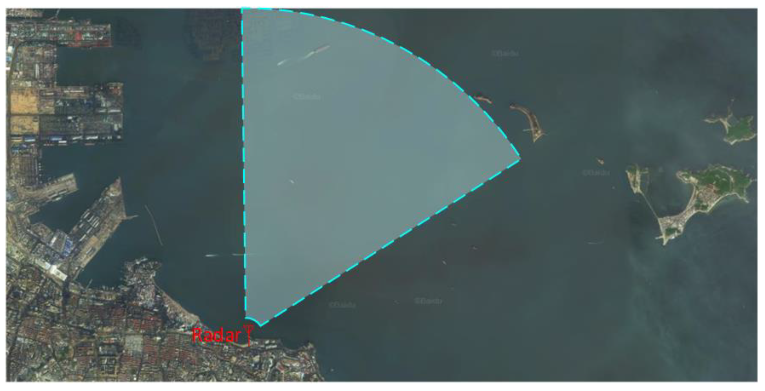
From 2019 to 2022, authors have proposed 6 issues in the SDRDSP database, including the radar cross-section (RCS) calibration, the observation of sea clutter under different sea conditions, and marine target detection. Since we focus on the sea clutter prediction, the first issue of the SDRDSP database in 2020 is employed in this paper to train and assess each prediction method. During the experiment in this issue, the radar is placed at a bathing beach in Yantai City, the altitude of the experiment scenario is about 400 m, and the height is 80 m [38]. Under different sea conditions, the radar works in the staring mode to observe sea clutter. The experimental scenario is shown in Figure 2, where the blue area indicates the area of observation.
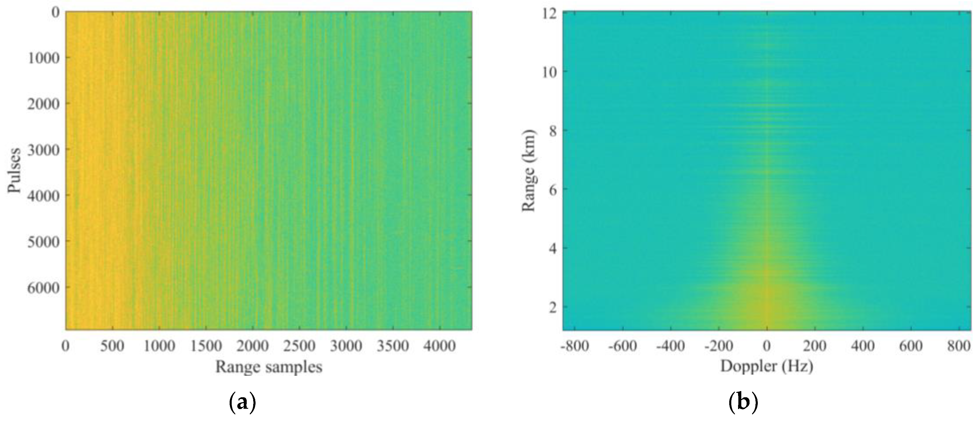
To be specific, the clutter-only “20210106155330_01_staring” dataset is employed to construct the training and test samples. Herein, the sea condition is 3~4 and there are no moving targets in the observation area due to the high sea condition. In addition, there are 6940 pulses of both the T1 and the T2 in this dataset, and there are 2224 and 4346 range samples of the T1 and T2, respectively. The pulse widths of the T1 and T2 are 0.04 and 3 , respectively. Since linear frequency modulation signals are more commonly used in advanced radar systems, we pay more attention to the T2 mode in the dataset and only samples in the T2 mode are used in the following experiments. For a visual understanding, the time-domain and range−Doppler map are given in Figure 3.
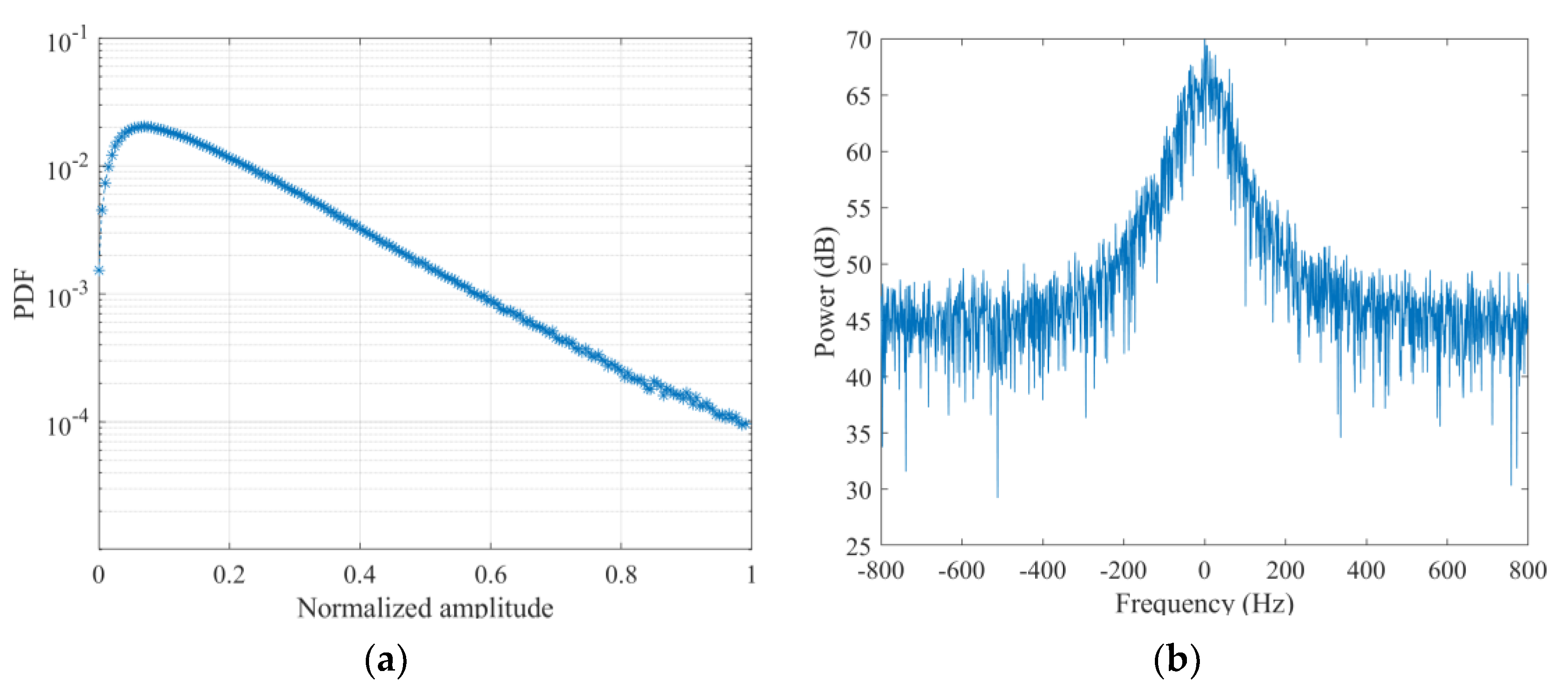
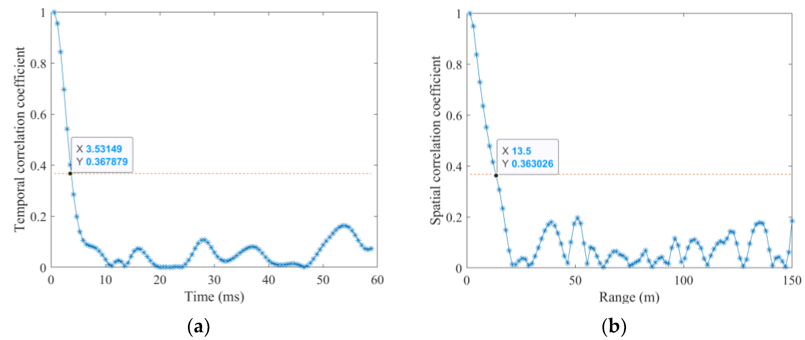
To further analyze the properties of the employed SDRDSP database, the measured amplitude distribution and the frequency spectrum are provided in Figure 4a,b, respectively. The amplitude distribution reveals a trailing phenomenon and the frequency spectrum indicates a Bragg peak near the zero frequency. The temporal and spatial correlations are shown in Figure 5a,b, respectively. By comparing with the threshold (shown as the red dotted line), the strong temporal correlation and spatial correlation are about 3.53 ms and 13.5 m, respectively.
3. Approach
In this section, a self-attention enhanced Seq2Seq structure is designed in this paper to tackle the k-step-ahead prediction problem. Considering that sea clutter is a chaotic time series, RNNs are still the backbone networks of the proposed structure inspired by the success of the previous prediction methods. Thus, the basis of RNNs and the inner structure of the proposed SCPNet are introduced, and details of the experiments are provided.
3.1. The Basis of RNNs
In feedforward neural networks, information and features of the current input are transferred unidirectionally. That is, the output of these networks only relies on the current input, which makes it easy for networks to train and optimize. While the output not only relies on the current input but also the previous outputs in many actual tasks. For example, it is difficult for feedforward neural networks to process time series, such as speech and text.
Different from feedforward neural networks, RNNs have loop structures and short-term memories, which indicates neurons in RNNs can receive information from both other neurons and self-neurons. Then RNNs are capable of processing time sequence data of any length by using neurons with self-feedback. For an input sequence , the hidden states in the corresponding hidden layer with self-feedback are updated as
where denotes the last hidden state and . is a nonlinear function or a feedforward neural network. That is, there are feedback connections between hidden states in RNNs, and these hidden states are capable of preserving memories and information from previous inputs.
Although plain RNNs can theoretically establish dependencies between states with long ranges, only short-term dependencies can be actually learned due to the problem of gradient explosion or vanishing gradient. To tackle this long-term dependency problem, the gating mechanism is introduced in RNNs to control the accumulating speed of information. The gating mechanism can selectively add new information and selectively forget previously accumulated information. Based on the gating mechanism, the LSTM and gated recurrent unit (GRU) are proposed. The GRU can be viewed as a slightly simplified LSTM cell, which provides less computational complexity [39].
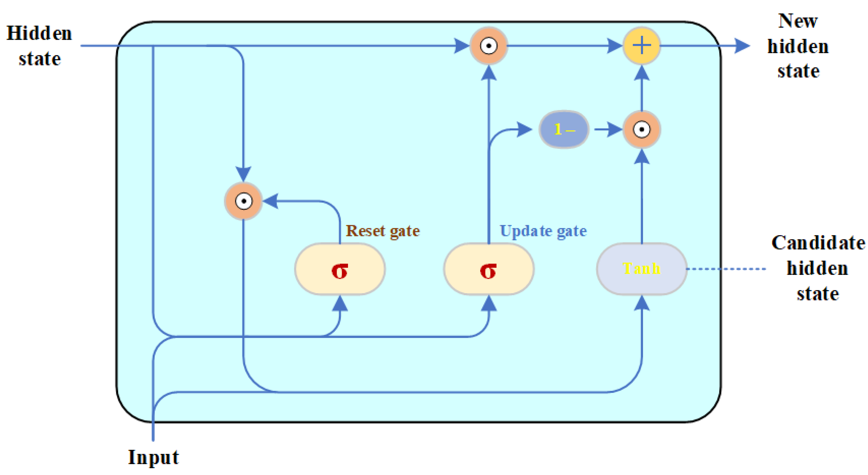
Different from plain RNNs, there are two gates in a GRU, namely, the reset gate and the update gate. These gates are capable of controlling hidden states and the values of their learnable parameters are between 0 to 1. Mathematically, for the same input in Equation (14), the reset gate is calculated as
where and denote the weights for input sequences and last hidden states, respectively; is the bias term and is the Sigmoid activation function. The reset gate actually controls the ratio of task-relevant previous states. Then the update gate is calculated as
where , , and denote the weights and the bias term, respectively.
The reset gate and last hidden states are then combined to calculate the current candidate hidden states as
where , , and denote the weights and the bias term, respectively. The “” is the Hadamard product. To combine the update gate and candidate hidden states, the current hidden states can be calculated as
For clarity, the reset gate is beneficial to catch the short-term dependency and the update gate is helpful to build the long-term dependency in sequences. The flowchart of a GRU is shown in Figure 6.
3.2. The Structure of the Proposed SCPNet
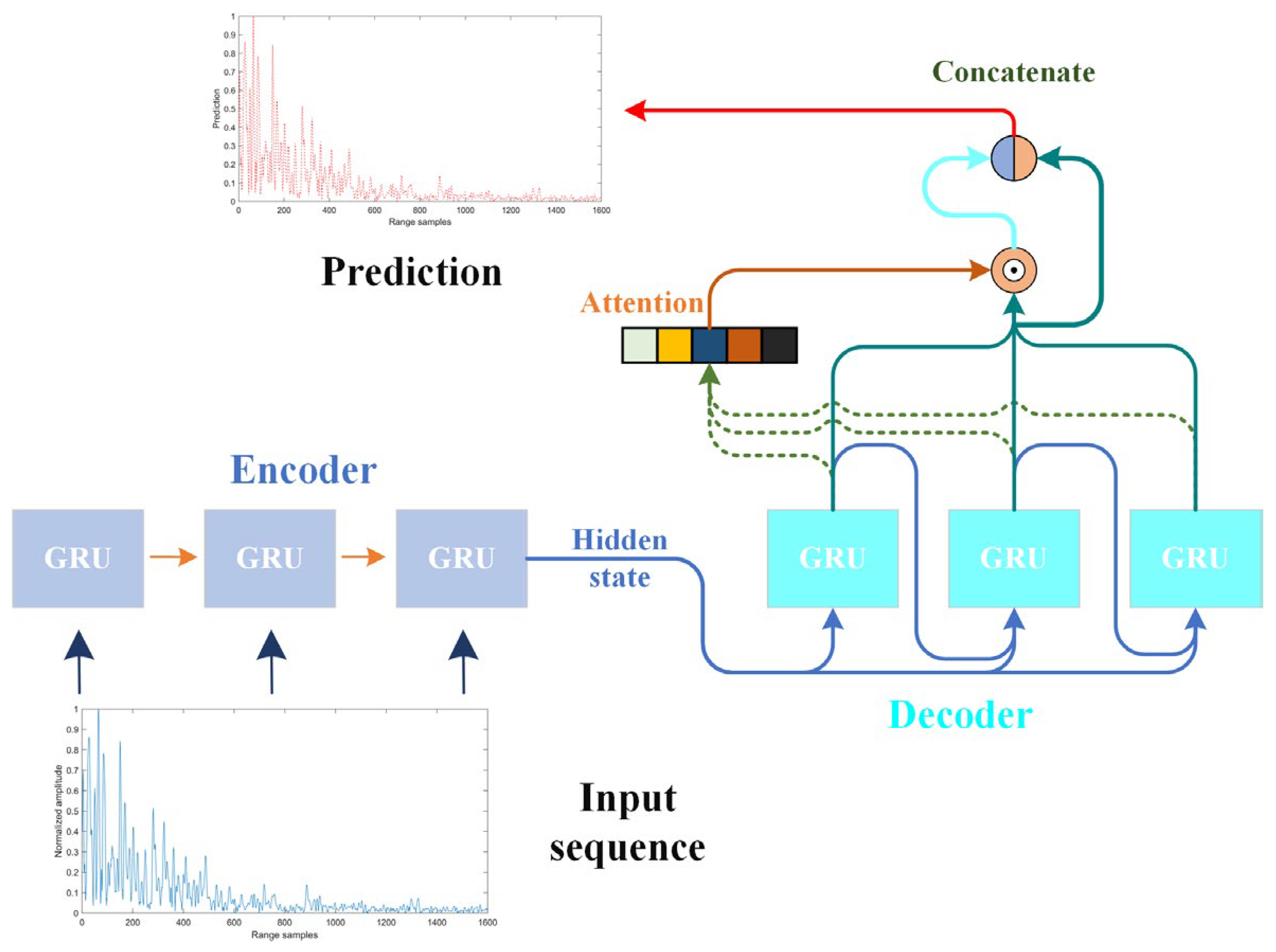
The proposed SCPNet consists of a Seq2Seq structure and a simple self-attention module, where the Seq2Seq structure is employed to tackle the k-step-ahead prediction and the self-attention module is capable of boosting the adaptive feature selection. First, the key to the k-step-ahead prediction is to construct a network where its input and output are sequences, and the length of the input sequence and output sequence can be different. For the input sequence and an output sequence , the goal of the Seq2Seq is to approximate the CPD as
where the subscript means the start and end of the sequence. Then, the maximum likelihood estimation can be used to find the optimization weight as follows,
Taking the time-series characteristics of sea clutter into consideration, two RNNs are employed in the SCPNet to construct a Seq2Seq model, where one RNN is used as an encoder and another is used as a decoder. For the encoder, the RNN can encode the input sequence to a matrix with a fixed dimension, and the vector usually is the hidden state at the last time step. That is,
where is the hidden state in the previous time step and is the learnable parameter in the encoder RNN.
Another RNN is then employed to encode and output the prediction sequence, where the initial hidden state is the hidden state in the last time step. That is,
at the t-th time step of the decoder, the current hidden state is
where is the hidden state in the previous time step and is the learnable parameter in the decoder RNN. Finally, the last hidden state of the decoder RNN is employed to obtain the prediction sequence via a linear layer.
Although the GRU and the Seq2Seq model improve the ability to build a long-term dependency, they are still prone to losing information from early stages if the input sequence is too long. Furthermore, the physical and chaotic characteristics of sea clutter are complex. It may be satisfactory for existing LSTM-based methods to achieve the one-step-ahead prediction, while the proposed SCPNet is required to not only build long-term dependency of the input sequence but also find time-series dependency of the prediction sequence with the length of k in the k-step-ahead prediction.
Thus, to further boost the feature adaptive selection ability, a simple self-attention module is introduced. The self-attention module is capable of constructing an external score to evaluate the significance of the output of each neuron at each moment in the GRU. The attention module aims to adaptively find task-relevant outputs and suppress useless features through the score function. A standard attention module always consists of a query, a key, and a value [24]. Mathematically, let denote the input of the attention module, the query matrix , the key matrix , and the value matrix are calculated as:
where , , and .
For each , the score is then calculated as:
where denotes the SoftMax function and is the score function. In the proposed SCPNet, the score function is achieved via a layer perceptron where the inputs are the outputs of the GRU in the decoder. The outputs of the GRU are then scaled by calculated scores.
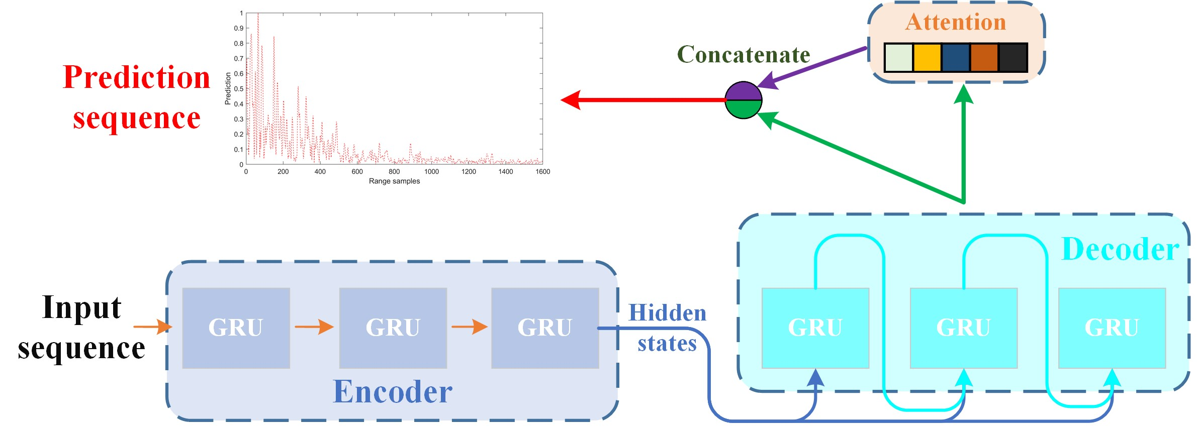
In the final layer of the proposed SCPNet, a linear layer is employed to map its inputs to the prediction sequence. To enrich the feature map, the scaled outputs of the decoder and the original outputs of the decoder are concatenated to serve as the inputs of the final linear layer. The detailed setting and structure of the proposed SCPNet are provided in Table 2, where “GRU 1 (Encoder)” means a GRU in the encoder part, the hidden size indicates the size of the hidden state, and “# Layers” means the number of layers. The flowchart of the proposed method is also shown in Figure 7, where “Concatenate” denotes the vector concatenation operation and “Attention” represents the attention module.
3.3. Details of Experiments
As mentioned above, the clutter-only “20210106155330_01_staring” dataset in the SDRDSP database is employed to construct the training and test samples. Since the T2 mode, namely, the linear frequency modulation mode, is much more commonly used than the single frequency mode in modern radar systems. The measured signals in the T2 mode are used and their absolute values are normalized to serve as the inputs of each method. In addition, due to the relatively weak amplitude of sea clutter far from the coast, only the first 1280 range samples of each pulse are selected for the sake of computational burden.
During the training of each method, a 2-norm gradient clipping method is employed to avoid the gradient exploding problem. The Adam [40] optimization algorithm is used to find the optimized weight of each method. Meanwhile, a cosine annealing warm restart is used for cooperative work with Adam to improve efficiency. As for the hyperparameters, the learning rate is 0.01, the batch size is 2048, and the number of epochs is 200. For all experiments, a server, equipped with a CPU of Intel Xeon Gold 6226R with a RAM of 256 G and a GPU of Nvidia Quadro RTX 6000 with a video memory of 24 G, is used. The software platform includes Python 3.8.5, PyTorch 1.7.1, and CUDA 11.0.
4. Results
In this subsection, the input length is selected through the results of the phase space reconstruction. Then, comparisons of the one-step-ahead prediction of the proposed method and the state-of-the-art methods are provided and analyzed. Moreover, comparisons of the one-step-ahead prediction and the computational complexity of each method are shown and discussed.
4.1. Results of the Phase Space Reconstruction
For a prediction method based on RNNs, the input length is an important hyper-parameter that is supposed to influence the prediction performance without a doubt. In many previous works focused on the sea clutter prediction problem, the optimized input length is selected manually by a series of experiments, which is inefficient and exhausting in practice. Fortunately, based on the phase space reconstruction theory, the optimized input length can be found due to the chaotic characteristics.
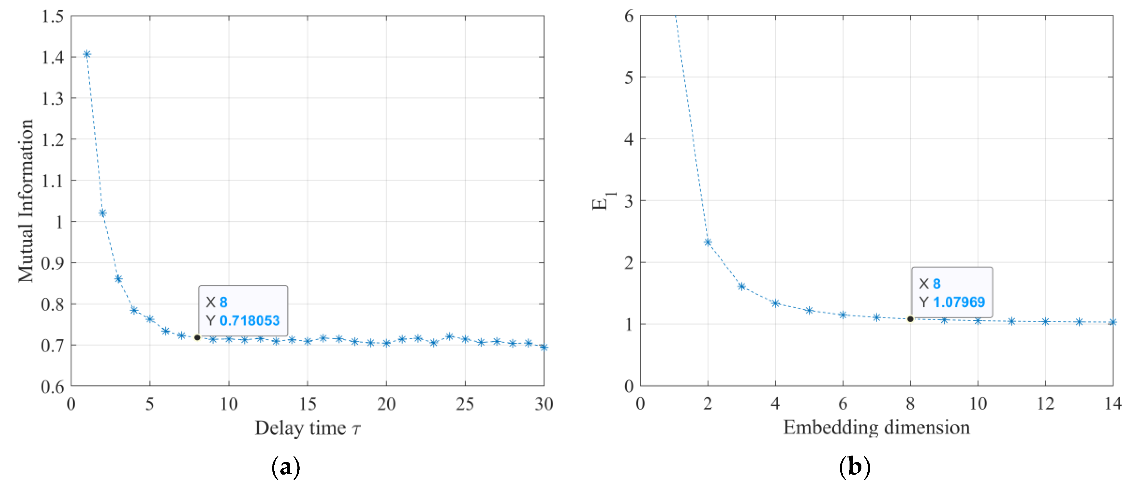
As mentioned in Section 2, the optimized length equals , just as indicated in Equation (4). The delay time is calculated through the mutual information algorithm, and the result is shown in Figure 8a. When the delay time is greater than eight, the mutual information is almost stable and no longer decreasing. Hence, the optimized delay time is eight. As for the optimized embedding dimension , it is selected by the Cao method and its result is shown in Figure 8b. Similarly, when the embedding dimension is greater than eight, the is no longer decreasing. Then the optimized embedding dimension is 8, which indicates the optimized input length is 64.
4.2. Comparisons on the One-Step-Ahead Prediction
Since the existing prediction methods are based on the one-step-ahead prediction, results with the one-step-ahead prediction of the proposed method and several state-of-the-art methods, including the GRNN, the DNN, the LSTM, and the GF-RNN, are compared and analyzed. Although the proposed method is designed for the k-step-ahead prediction, the proposed method can be easily converted to the one-step-ahead prediction. To be specific, if the input sequence and the interval of each input sequence are the same as the existing methods, the proposed method can be viewed as the one-step-ahead prediction by only using the first prediction value in each prediction.
As for the metrics of comparisons, except for the MSE defined in Equation (7), the mean absolute error (MAE) is also employed to evaluate the performance, which is defined as
where denotes the absolute value function. The MSE and MAE of each method are provided in Table 3, where results are in the format of average standard deviation.
For the one-step-ahead prediction, the MSE and the MAE of the SCPNet are about 1.48 × 10⁻⁵ and 2.25 × 10⁻³, respectively. That is, the proposed SCPNet is capable of achieving the smallest MSE and MAE, which indicates the SCPNet can still have the best prediction performance compared with the four existing methods. In addition, compared with the GRNN and the DNN, the RNN-based networks, namely, the SCPNet, the LSTM, and the GF-RNN, obviously gain better prediction performance, which verifies the superiority of RNNs.
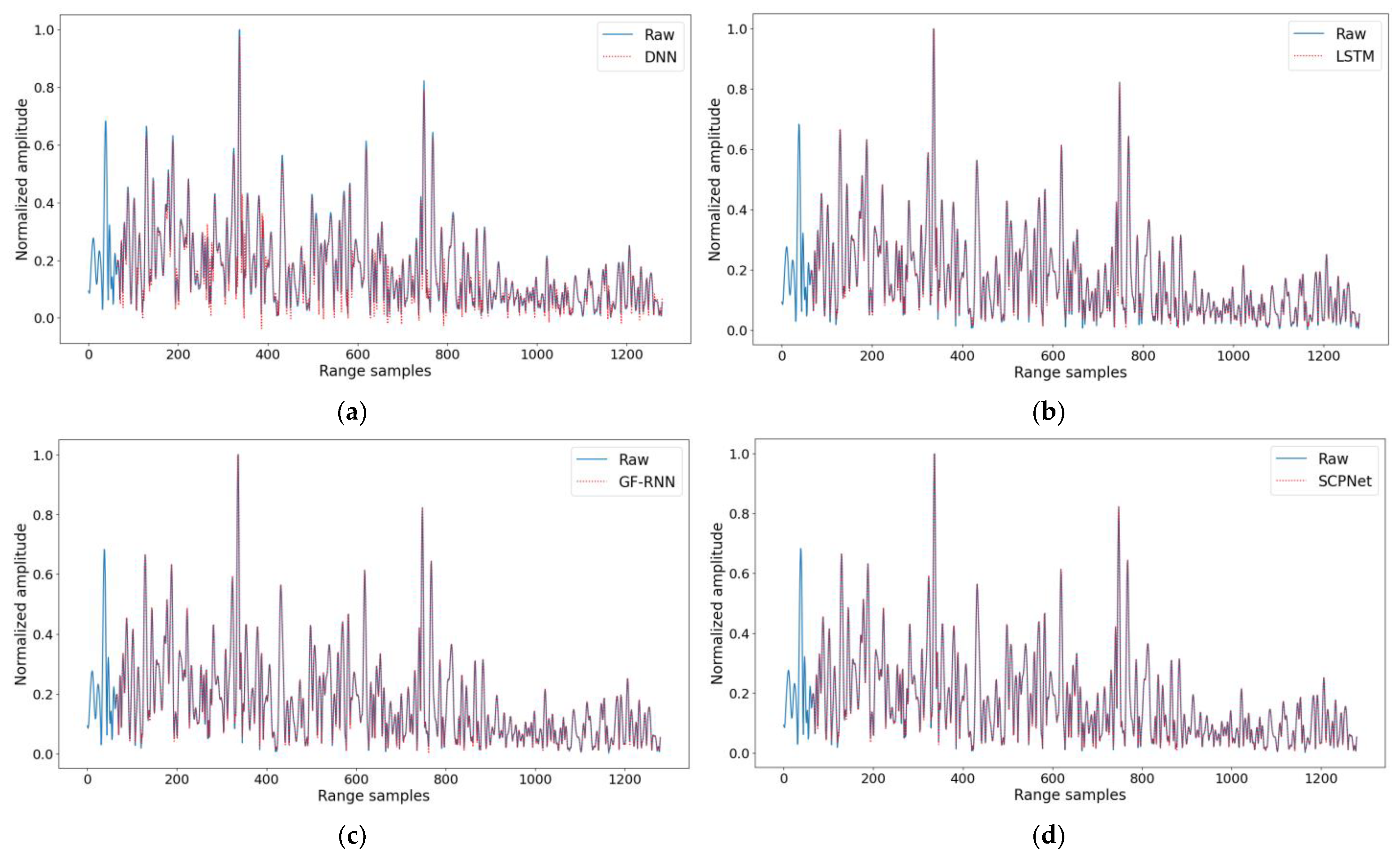
For a visible comparison, the prediction result of each method is shown in Figure 9, where “Raw” denotes the ground truth of sea clutter and red points are the prediction results of each method. Due to the poor prediction performance of the GRNN, its result is not provided herein. Overall, four methods are capable of fitting the variation trend of sea clutter, but there are a lot of prediction errors of the DNN and the LSTM at the bottom of the sea clutter. The prediction performance of the proposed SCPNet is slightly better than that of the GF-RNN in this clutter sample. To summarize, it is not a difficult task to achieve the one-step-ahead prediction of existing RNN-based methods, and the proposed SCPNet has the best prediction performance.
4.3. Comparisons on the k-Step-Ahead Prediction
In the k-step-ahead prediction, the prediction method is required to predict the k value in one prediction. For those existing methods, it is a viable way to use the recursive one-step-ahead prediction and then achieve the k-step-ahead prediction indirectly. The proposed method uses the Seq2Seq structure to directly achieve the k-step-ahead prediction. Then, the results on the k-step-ahead prediction are analyzed and discussed. Table 4 shows the MSE of each method with different k in the k-step-ahead prediction.
For clarity, only three RNN-based methods are compared in Table 4. When k is 1, it then becomes the one-step-ahead prediction. When k equals 2, the MSE of the proposed SCPNet is 1.35 × 10⁻⁴ which is about 0.56 × 10⁻⁴ and 1.4 × 10⁻⁴ lower than that of the GF-RNN and the LSTM, respectively. Compared with the MSE of the one-step-ahead prediction, the MSE of each method is remarkably decreased when k = 2. Even for the proposed method, the MSE is about 1.2 × 10⁻⁴ higher compared with the one-step-ahead prediction. When k is gradually increasing, the MSE of each method is also increasing. However, no matter what k is, the MSE of the proposed SCPNet is the lowest compared to that of the GF-RNN and the LSTM. It is of note that the MSE of the LSTM is dramatically decreased when k = 32, which is because prediction errors are supposed to be accumulated in the recursive one-step-ahead prediction.
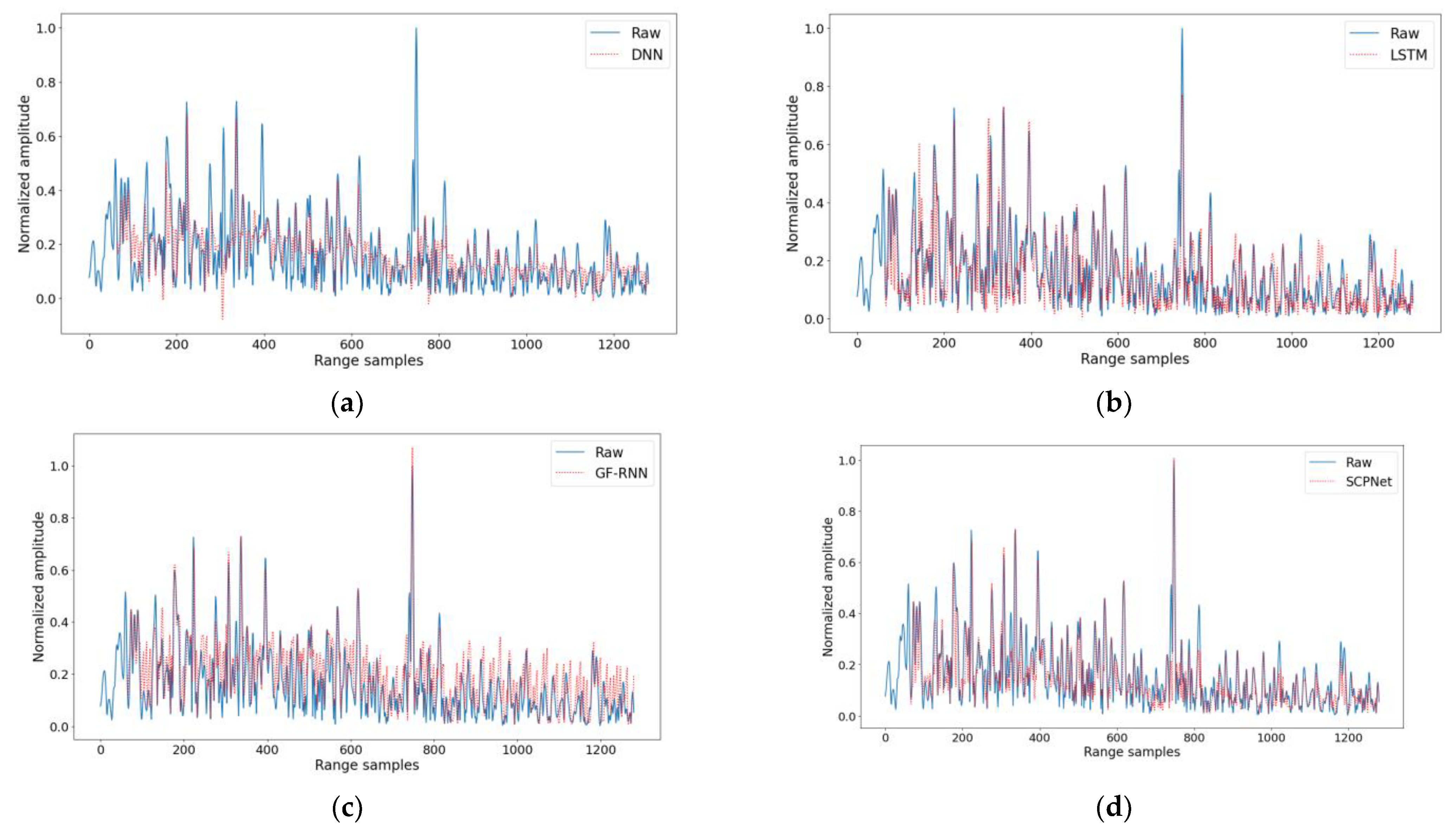
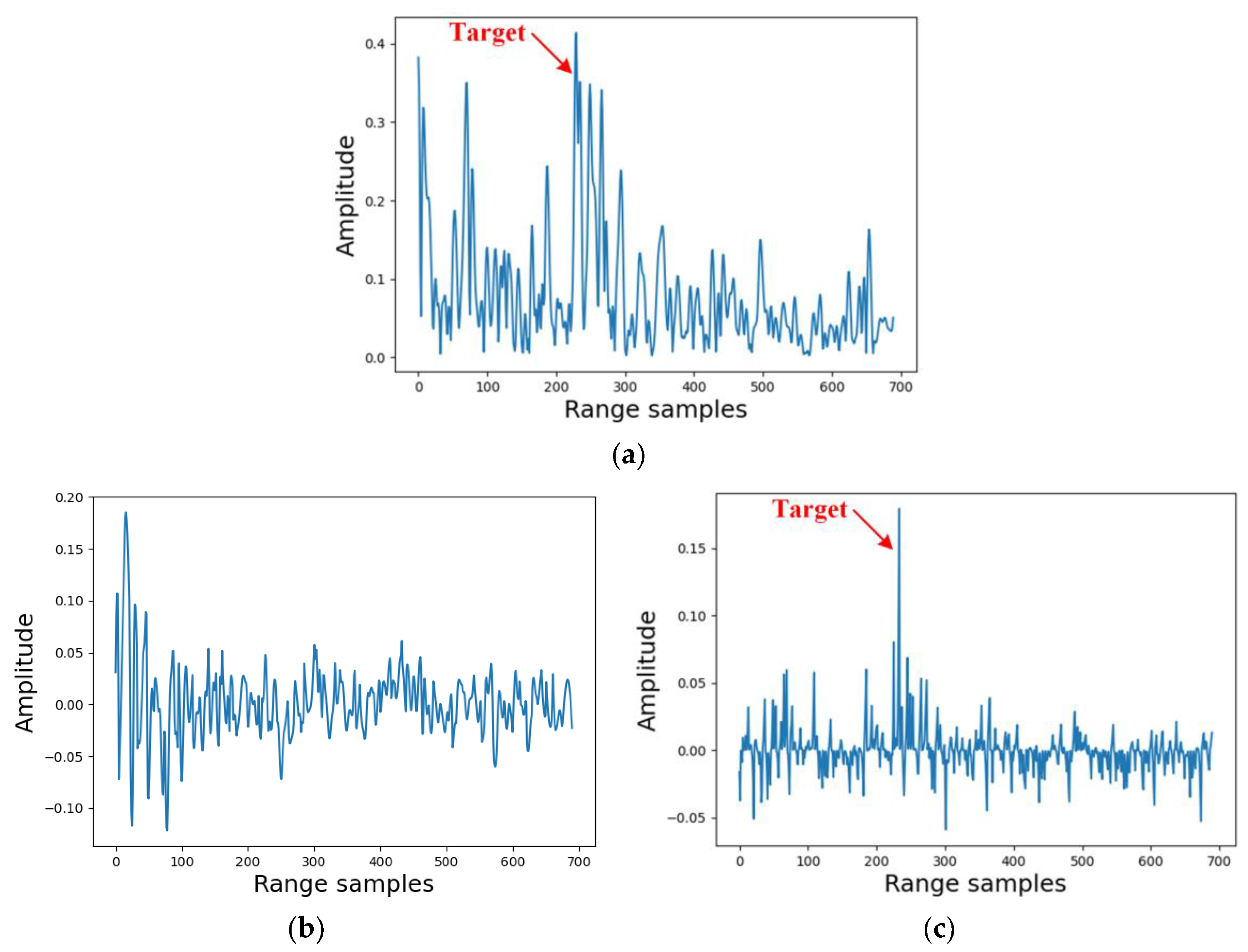
For a visible comparison, the prediction result when k is 8 of each method is shown in Figure 10. The prediction sequence of the DNN can hardly fit the raw clutter sequence, even the prominent peak has not been predicted by the DNN. As for the LSTM, the prediction peak is also much lower than the raw peak and there are a lot of prediction errors at the bottom of the clutter sequence. The prediction peak of the GR-RNN, nevertheless, is higher than the raw clutter sequence. Moreover, there are a large number of false peaks around fluctuations of the raw clutter sequence, which means there will be lots of false high values in the prediction sequence. As for the proposed SCPNet, it can fit most peaks and fluctuations of the raw clutter sequence and there are only a few false high values in the prediction sequence, which verifies the superiority of the proposed method in the k-step-ahead prediction.
5. Discussions
5.1. The Consistency Analysis
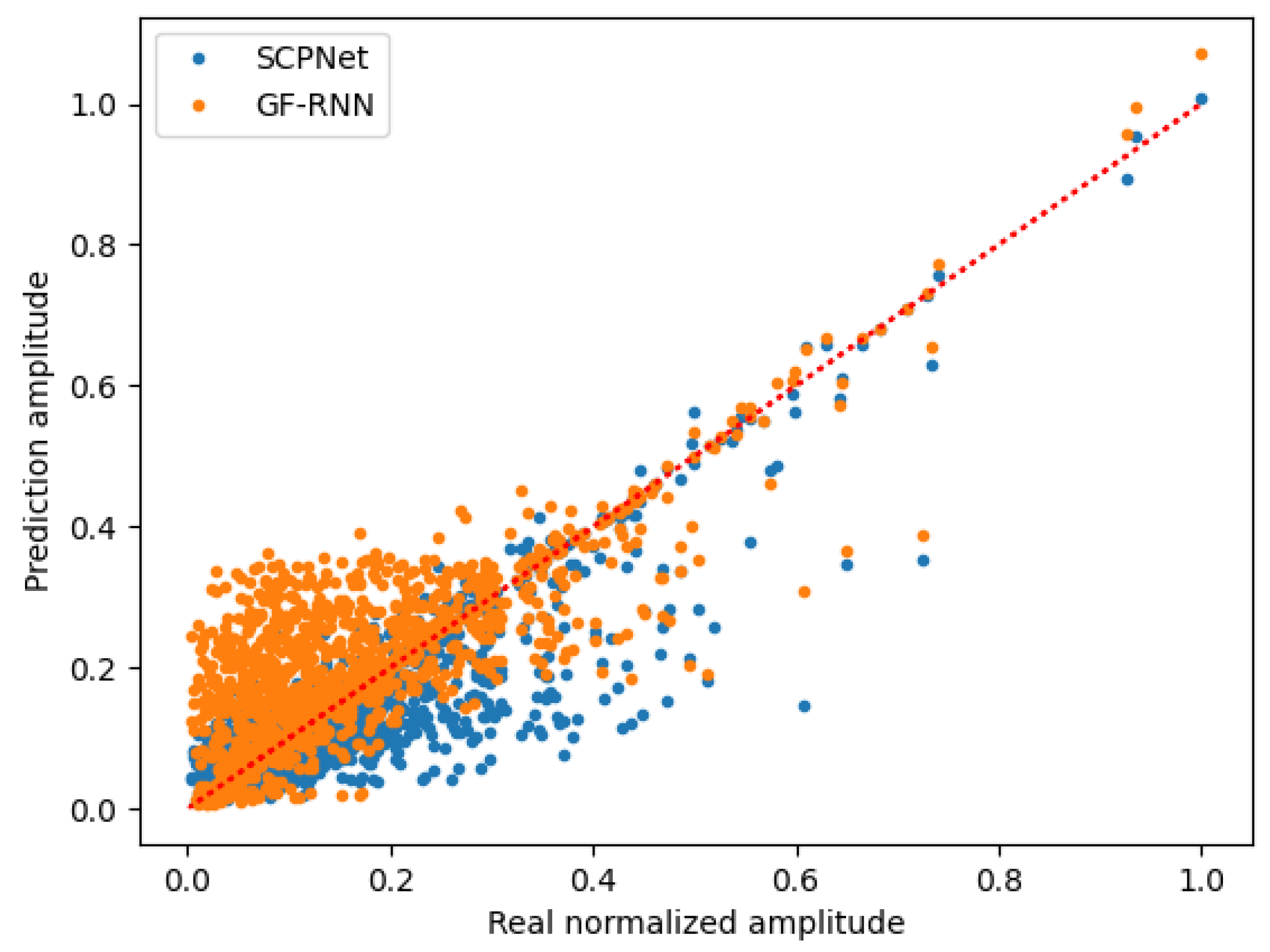
Furthermore, to evaluate the prediction results in depth, the consistency between the predictions and raw clutter sequence is analyzed and shown in Figure 11, where the state-of-the-art GF-RNN is compared. Herein, the red dotted line denotes the prediction results equal to the raw clutter sequence. Hence, fewer outliers away from the red dotted line indicate better prediction performance. The prediction results of both of the two methods are more located under the normalized amplitude of 0.5. In the area of the real normalized amplitude of 0 to 0.3, the blue points of the SCPNet are more concentrated around the red dotted line than the orange points of the GF-RNN.
Most outliers of the SCPNet are located at the low right part and under the red dotted line, which means false predictions of the SCPNet tend to be lower than the real values. On the contrary, most outliers of the GF-RNN are located in the upper left part, which indicates false predictions of the GF-RNN tend to be higher than the real values. Taking the time-domain cancellation into consideration, if the prediction sequence is higher than the real clutter, the amplitude of the target of interest would also be weakened falsely, which is prone to losing targets in the following detection step.
To conclude, it is more challenging to achieve the k-step-ahead prediction compared with the one-step-ahead prediction. When the k is gradually becoming greater, prediction errors of each method are also increasing. Especially for the recursive one-step-ahead pre-diction, prediction errors are supposed to be accumulated, which causes remarkable performance degradation. On the other hand, the proposed SCPNet achieves better prediction performance on the k-step-ahead prediction compared with existing methods.
Since the characteristics of input sea clutter under kinds of sea conditions are different as well. To be specific, amplitude distributions of sea clutter are supposed to change with different sea conditions and observation areas, and some environmental parameters, including the wind velocity, will also have an impact on the spectrum of sea clutter. On the other hand, the proposed method based on supervised learning requires that the training dataset and the test dataset should conform to the same distribution so that the learning method can achieve better performance. Sea clutter with different characteristics obviously does not belong to the same distribution. Thus, the accuracy of prediction is supposed to be related to the distributions and the spectrum of sea clutter. For the sake of further applications, the proposed method can be improved via transfer learning under different distributions and spectrums of clutter.
5.2. The Performance of Target Detection
As pointed out in the introduction, the aim of the proposed method is to use extrapolated clutter sequence to detect the presence of a target through time cancellation. In the radar community, the MTI is a well-known and widely used clutter-suppression method based on time cancellation. To demonstrate the performance of clutter suppression and target detection, a target-containing dataset, namely, the “20210106160919_01_staring” dataset is employed to verify the performance of both the proposed method and the MTI method. The raw echo sequence and detection results are shown in Figure 12. Herein, the MTI indicates a three-pulse-cancellation MTI method.
In Figure 12a, the target of interest is partly covered by the wild clutter and it is very challenging to detect the target while keeping a satisfactory probability of false alarm. Although wild clutter amplitudes are greatly decreased after the MTI method, the target of interest is drastically suppressed as well due to the low speed of the target. As for the result of the proposed method, most wild clutter amplitudes are suppressed while the target is retained. Compared with the raw sequence, the target of the proposed method is much more distinguished, which is supposed to be beneficial to target detection.
5.3. The Computational Complexity
For the sake of practical applications, it is also necessary to analyze the computational complexity of each method. Herein, three metrics are employed to measure the computational complexity, including the inference time, the floating-point operations (FLOPs), and the learnable parameters. The inference time is the consuming time of one prediction on the above-mentioned hardware platform, the FLOPs are widely used to measure the complexity of a neural network, and the learnable parameters indicate the number of learnable data in a neural network.
The computational complexity of each method is listed in Table 5. The inference time of the proposed SCPNet is about 9.8 ms, the FLOPs are 1685 K, and the SCPNet has about 23 K learnable parameters. Although the DNN has the lowest computational complexity in Table 5, the prediction performance of the DNN in the k-step-ahead prediction is the worst. The computational complexity of the GF-RNN and the LSTM is also lower than that of the proposed SCPNet, while the inference time of the SCPNet is only 2 ms more than that of the GF-RNN. More importantly, the computational complexity of the SCPNet is actually based on a 32-step-ahead prediction. That is, based on the computational complexity listed in Table 5, the SCPNet can predict 32 values in one prediction while the rest of the methods only predict one value. Hence, the proposed method is still more efficient than the GF-RNN in practice.
6. Conclusions
In this paper, an attention-enhanced Seq2Seq structure is designed to achieve both the one-step-ahead prediction and the k-step-ahead prediction. The proposed SCPNet takes full advantage of the powerful ability of the Seq2Seq model in the time-series processing and the adaptive feature selection of the self-attention module. In addition, the phase space reconstruction theory is employed to find the optimized input sequence. Results with the SDRDSP database demonstrate that the proposed SCPNet is capable of achieving the lowest MSE in both the one-step-ahead prediction and the k-step-ahead prediction, which verifies that the proposed method outperforms the GRNN, the DNN, the LSTM, and the GF-RNN. The analysis of the computational complexity shows the proposed method takes relatively more FLOPs and parameters while the proposed method is still more efficient in practice. The promising results of the proposed method also underscore the potential of the Seq2Seq structure in the k-step-ahead prediction of sea clutter.
Author Contributions
Conceptualization, Q.Q. and H.C.; methodology, Q.Q.; software, Q.Q. and Z.L.; validation, B.L., Q.D. and Y.W.; writing—original draft preparation, Q.Q.; writing—review and editing, H.C., Z.L. and Y.W.; funding acquisition, B.L. All authors have read and agreed to the published version of the manuscript.
Funding
This work was supported by the National Natural Science Foundation of China under Grants 62001510.
Data Availability Statement
Not Applicable.
Conflicts of Interest
The authors declare no conflict of interest.
References
- Chen, X.; Su, N.; Huang, Y.; Guan, J. False-alarm-controllable radar detection for marine target based on multi features fusion via CNNs. IEEE Sens. J. 2021, 21, 9099–9111. [Google Scholar] [CrossRef]
- Lei, Z.; Chen, H.; Zhang, Z.; Dou, G.; Wang, Y. A cognitive beamforming method via range-Doppler map feature for skywave radar. Remote Sens. 2022, 14, 2879. [Google Scholar] [CrossRef]
- Zhang, T.; Wang, Z.; Xing, M.; Zhang, S.; Wang, Y. Research on multi-domain dimensionality reduction joint adaptive processing method for range ambiguous clutter of FDA-Phase-MIMO space-based early warning radar. Remote Sens. 2022, 14, 5536. [Google Scholar] [CrossRef]
- Lv, M.; Zhou, C. Study on sea clutter suppression methods based on a realistic radar dataset. Remote Sens. 2019, 11, 2721. [Google Scholar] [CrossRef] [Green Version]
- Xie, H. Sea Clutter Suppression Method Based on Complex-Valued Neural Network. Master’s Thesis, University of Electronic Science and Technology of China, Chengdu, China, 2022. [Google Scholar]
- Poon, M.W.Y. A Clutter Suppression Scheme for High Frequency (HF) Radar. Master’s Thesis, Memorial University of Newfoundland, St. John’s, NL, Canada, 1991. [Google Scholar]
- Jangal, F.; Saillant, S.; Hélier, M. Ionospheric clutter cancellation and wavelet analysis. In Proceedings of the European Conference on Antennas and Propagation, Nice, France, 6–10 November 2006; pp. 1–6. [Google Scholar]
- Huang, N.E.; Zheng, S.; Steven, R.I. A new view of nonlinear water waves: The Hilbert spectrum. Annu. Rev. Fluid Mech 1999, 31, 417–457. [Google Scholar] [CrossRef] [Green Version]
- Qu, Q.; Wang, Y.-L.; Liu, W.; Li, B. A false alarm controllable detection method based on CNN for sea-surface small targets. IEEE Geosci. Remote Sens. Lett. 2022, 19, 1–5. [Google Scholar] [CrossRef]
- Rosenberg, L.; Watts, S. Radar Sea Clutter: Modelling and Target Detection; Institution of Engineering and Technology: London, UK, 2022; pp. 32–38. [Google Scholar]
- Haykin, S.; Leung, H. Model reconstruction of chaotic dynamics: First preliminary radar results. In Proceedings of the ICASSP-92: 1992 IEEE International Conference on Acoustics, Speech, and Signal Processing, San Francisco, CA, USA, 23–26 March 1992; pp. 125–128. [Google Scholar] [CrossRef]
- Leung, H.; Lo, T. Chaotic radar signal processing over the sea. IEEE J. Ocean. Eng. 1993, 18, 287–295. [Google Scholar] [CrossRef]
- Li, B.; Haykin, S. Chaotic detection of small target in sea clutter. In Proceedings of the 1993 IEEE International Conference on Acoustics, Speech, and Signal Processing, Minneapolis, MN, USA, 27–30 April 1993; pp. 237–240. [Google Scholar] [CrossRef]
- Leung, H. Nonlinear clutter cancellation and detection using a memory-based predictor. IEEE Trans. Aerosp. Electron. Syst. 1996, 32, 1249–1256. [Google Scholar] [CrossRef]
- Xie, N.; Leung, H.; Chan, H. A multiple-model prediction approach for sea clutter modeling. IEEE Trans. Geosci. Remote Sens. 2003, 41, 1491–1502. [Google Scholar] [CrossRef]
- Jiang, B.; Wang, H.; Fu, Y.; Li, X.; Guo, G.R. Prediction of sea clutter chaotic time series using LS-SVM. Prog. Nat. Sci. 2007, 17, 415–420. (In Chinese) [Google Scholar]
- Gao, Z.; Chen, L. Sea clutter sequences regression prediction based on PSO-GRNN method. In Proceedings of the 2015 8th International Symposium on Computational Intelligence and Design (ISCID), Hangzhou, China, 12–13 December 2015; pp. 72–75. [Google Scholar] [CrossRef]
- Cognitive Systems Laboratory, McMaster University, Canada. The IPIX Radar Database. Available online: http://soma.mcmaster.ca//ipix.php (accessed on 28 February 2022).
- Xing, H.; Yan, Y. Detection of low-flying target under the sea clutter background based on Volterra filter. Complexity 2018, 12, 591. [Google Scholar] [CrossRef] [Green Version]
- Chen, Z.; Tian, B.; Zhang, S.; Xu, Q. quantitative prediction of sea clutter power based on improved grey Markov model. Atmosphere 2022, 13, 1085. [Google Scholar] [CrossRef]
- Qu, Q.; Wei, S.; Liu, S.; Liang, J.; Shi, J. JRNet: Jamming recognition networks for radar compound suppression jamming signals. IEEE Trans. Veh. Technol. 2020, 69, 15035–15045. [Google Scholar] [CrossRef]
- Wei, S.; Qu, Q.; Zeng, X.; Liang, J.; Shi, J.; Zhang, X. Self-Attention Bi-LSTM networks for radar signal modulation recognition. IEEE Trans. Microw. Theory Tech. 2021, 69, 5160–5172. [Google Scholar] [CrossRef]
- Qu, Q.; Wang, Y.-L.; Liu, W.; Wei, S.; Du, Q. IRNet: Interference recognition networks for automotive radars via autocorrelation features. IEEE Trans. Microw. Theory Tech. 2022, 70, 2762–2774. [Google Scholar] [CrossRef]
- Qiu, X. Neural Networks and Deep Learning; Machine Press: Beijing, China, 2020; pp. 131–135. [Google Scholar]
- Hochreiter, S.; Schmidhuber, J. Long short-term memory. Neural Comput. 1997, 9, 1735–1780. [Google Scholar] [CrossRef] [PubMed]
- Zhao, J.; Wu, J.; Guo, X.; Han, J.; Yang, K.; Wang, H. Prediction of radar sea clutter based on LSTM. J. Ambient. Intell. Human Comput. 2019, 335, 4. [Google Scholar] [CrossRef]
- Ma, L.; Wu, J.; Zhang, J.; Wu, Z.; Jeon, G.; Tan, M.; Zhang, Y. Sea clutter amplitude prediction using a long short-term memory neural network. Remote Sens. 2019, 11, 2826. [Google Scholar] [CrossRef] [Green Version]
- Chen, X.; Wu, J.; Guo, X. Prediction of sea clutter characteristics by deep neural networks using marine environmental factors. Environ. Dev. Sus. 2022, 26, 1–20. [Google Scholar] [CrossRef]
- Ma, L.; Zhang, J.; Wu, J.; Zhang, Y.; Zhao, P.; Xia, X. Prediction of sea clutter using gated feedback recurrent neural network. Chin. J. Radio Sci. 2020, 35, 257–263. (In Chinese) [Google Scholar]
- Liu, N.; Dong, Y.; Wang, G.; Ding, H.; Huang, Y.; Guan, J.; Chen, X.L.; He, Y. Sea-detecting X-band radar and data acquisition program. J. Radars 2019, 8, 656–667. [Google Scholar] [CrossRef]
- Ding, H.; Dong, Y.; Liu, N.; Wang, G.; Guan, J. Overview and prospects of research on sea clutter property cognition. J. Radars 2016, 5, 499–516. [Google Scholar] [CrossRef]
- Khan, R.H. Ocean-clutter model for high-frequency radar. IEEE J. Ocean. Eng. 1991, 16, 181–188. [Google Scholar] [CrossRef]
- Ma, L. Research on Sea Clutter Characteristics Based on Deep Learning and Marine Environmental Parameters. Ph.D.’s Thesis, Xidian University, Shanxi, China, 2020. [Google Scholar]
- Takens, F. Detecting strange attractors in turbulence. In Lecture Notes in Mathematics; Morel, J.M., Teissier, B., Eds.; Springer: Cham, Switzerland, 1981; pp. 366–381. [Google Scholar]
- He, K. Research on Sea Clutter Suppression Method of HFSWR Based on RBF Neural Network. Master’s Thesis, Jiangsu University of Science and Technology, Zhenjiang, China, 2021. [Google Scholar]
- Hornik, K.; Stinchcombe, M.; White, H. Multilayer Feedforward Networks Are Universal Approximators. Neural Netw. 1989, 2, 359–366. [Google Scholar] [CrossRef]
- Cao, L. Practical Method for Determining the Minimum Embedding Dimension of a Scalar Time Series. Phys. Rev. 1997, 110, 43–50. [Google Scholar] [CrossRef]
- Liu, N.; Ding, H.; Huang, Y.; Dong, Y.L.; Wang, G.Q.; Dong, K. Annual progress of the sea-detecting X-band radar and data acquisition program. J. Radars 2021, 10, 173–182. [Google Scholar] [CrossRef]
- Chung, J.; Gulcehre, C.; Cho, K.; Bengio, Y. Gated feedback recurrent neural networks. In Proceedings of the 32nd International Conference on Machine Learning (ICML), Lille, France, 6–11 July 2015; pp. 2067–2075. [Google Scholar]
- Kingma, D.; Ba, J. Adam: A method for stochastic optimization. In Proceedings of the 3rd International Conference on Learning Representations (ICLR), San Diego, CA, USA, 7–9 May 2015. [Google Scholar]
Figure 1.
The difference between the one-step-ahead prediction and the k-step-ahead prediction. (a) the one-step-ahead prediction; (b) the k-step-ahead prediction.
Figure 1.
The difference between the one-step-ahead prediction and the k-step-ahead prediction. (a) the one-step-ahead prediction; (b) the k-step-ahead prediction.

Figure 2.
The diagram of the experimental scene in the Baidu map. The blue area indicates the area of observation.
Figure 2.
The diagram of the experimental scene in the Baidu map. The blue area indicates the area of observation.

Figure 3.
The time domain and range−Doppler map of the selected dataset. (a) the time domain of the T2; (b) the range−Doppler map of the T2.
Figure 3.
The time domain and range−Doppler map of the selected dataset. (a) the time domain of the T2; (b) the range−Doppler map of the T2.

Figure 4.
The amplitude distribution and the frequency spectrum of the employed database. (a) the amplitude distribution; (b) the frequency spectrum.
Figure 4.
The amplitude distribution and the frequency spectrum of the employed database. (a) the amplitude distribution; (b) the frequency spectrum.

Figure 5.
The temporal correlation and the spatial correlation of the employed database. (a) the temporal correlation; (b) the spatial correlation.
Figure 5.
The temporal correlation and the spatial correlation of the employed database. (a) the temporal correlation; (b) the spatial correlation.

Figure 6.
The flowchart of a GRU.

Figure 7.
The flowchart of the proposed method.

Figure 8.
The results of the phase space reconstruction. (a) the delay time ; (b) the embedding dimension .
Figure 8.
The results of the phase space reconstruction. (a) the delay time ; (b) the embedding dimension .

Figure 9.
The prediction result of each method on the one-step-ahead prediction. (a) the DNN; (b) the LSTM; (c) the GF-RNN; (d) the proposed SCPNet.
Figure 9.
The prediction result of each method on the one-step-ahead prediction. (a) the DNN; (b) the LSTM; (c) the GF-RNN; (d) the proposed SCPNet.

Figure 10.
The prediction result of each method on the 8-step-ahead prediction. (a) the DNN; (b) the LSTM; (c) the GF-RNN; (d) the proposed SCPNet.
Figure 10.
The prediction result of each method on the 8-step-ahead prediction. (a) the DNN; (b) the LSTM; (c) the GF-RNN; (d) the proposed SCPNet.

Figure 11.
The consistency between prediction methods and the raw clutter sequence.

Figure 12.
The raw echo sequence and detection results. (a) the raw sequence; (b) the detection result of the MTI method; (c) the detection result of the proposed method.
Figure 12.
The raw echo sequence and detection results. (a) the raw sequence; (b) the detection result of the MTI method; (c) the detection result of the proposed method.


Table 1.
The detailed physical parameters of the employed radar in the SDRDSP database.
| Name | Value |
|---|---|
| Frequency | 9.3~9.5 GHz |
| Bandwidth | 25 MHz |
| Range resolution | 6 m |
| Pulse repetition frequency | 1.6 kHz |
| Peak power | 50 W |
| Antenna length | 1.8 m |
| Polarization mode | HH |
| Operation mode | Staring or scan |
| Horizontal beam width | 1.2° |
| Grazing angle | 1.2°~7° |
| Transmitting signal | Single frequency pulse Linear frequency modulation pulse |
Table 2.
The detailed structure of the proposed SCPNet.
| Layer | Input Size | Output Size | Hidden Size | Activation | # Layers |
|---|---|---|---|---|---|
| GRU 1 (Encoder) | 1 | 32 | 32 | Sigmoid Tanh | 1 |
| GRU 2 (Encoder) | 32 | 32 | 32 | Sigmoid Tanh | 1 |
| GRU 3 (Decoder) | 32 | 32 | 32 | Sigmoid Tanh | 1 |
| GRU 4 (Decoder) | 32 | 32 | 32 | Sigmoid Tanh | 1 |
| Linear 1 (Attention) | 32 | 32 | - | SoftMax | 1 |
| Linear 2 (Output) | 64 | 32 | - | - | 1 |
Table 3.
The MSE and MAE of each method.
| SCPNet (Proposed) | GRNN | DNN | LSTM | GF-RNN | |
|---|---|---|---|---|---|
| MSE | 1.48 × 10⁻⁵ ±5.2 × 10⁻⁶ | 1.87 × 10⁻² ±5.1 × 10⁻³ | 1.02 × 10⁻³ ±2.6 × 10⁻⁴ | 3.55 × 10⁻⁵ ±6.2 × 10⁻⁶ | 1.72 × 10⁻⁵ ±5.1 × 10⁻⁶ |
| MAE | 2.25 × 10⁻³ ±3.6 × 10⁻⁴ | 9.9 × 10⁻² ±1.4 × 10⁻² | 2.02 × 10⁻² ±3.3 × 10⁻³ | 3.71 × 10⁻³ ±3.8 × 10⁻⁴ | 2.85 × 10⁻³ ±3.5 × 10⁻⁴ |
Table 4.
The MSE of each method with different k.
| k = 1 | k = 2 | k = 4 | k = 8 | k = 16 | k = 32 | |
|---|---|---|---|---|---|---|
| SCPNet (Proposed) | 1.48 × 10⁻⁵ | 1.35 × 10⁻⁴ | 1.39 × 10⁻³ | 8.76 × 10⁻³ | 0.016 | 0.021 |
| LSTM | 3.55 × 10⁻⁵ | 2.75 × 10⁻⁴ | 2.76 × 10⁻³ | 0.015 | 0.058 | 0.313 |
| GF-RNN | 1.72 × 10⁻⁵ | 1.91 × 10⁻⁴ | 2.23 × 10⁻³ | 0.011 | 0.024 | 0.035 |
Table 5.
The computational complexity of each method.
| SCPNet (Proposed) | GF-RNN | LSTM | DNN | |
|---|---|---|---|---|
| Time (ms) | 9.8 | 7.8 | 3 | 0.6 |
| FLOPs (K) | 1685 | 246 | 305 | 1.3 |
| Parameter (K) | 23 | 3.5 | 4.5 | 1.2 |
Disclaimer/Publisher’s Note: The statements, opinions and data contained in all publications are solely those of the individual author(s) and contributor(s) and not of MDPI and/or the editor(s). MDPI and/or the editor(s) disclaim responsibility for any injury to people or property resulting from any ideas, methods, instructions or products referred to in the content. |
© 2023 by the authors. Licensee MDPI, Basel, Switzerland. This article is an open access article distributed under the terms and conditions of the Creative Commons Attribution (CC BY) license (https://creativecommons.org/licenses/by/4.0/).
Share and Cite
MDPI and ACS Style
Qu, Q.; Chen, H.; Lei, Z.; Li, B.; Du, Q.; Wang, Y. Sea Clutter Amplitude Prediction via an Attention-Enhanced Seq2Seq Network. Remote Sens. 2023, 15, 3234. https://doi.org/10.3390/rs15133234
AMA Style
Qu Q, Chen H, Lei Z, Li B, Du Q, Wang Y. Sea Clutter Amplitude Prediction via an Attention-Enhanced Seq2Seq Network. Remote Sensing. 2023; 15(13):3234. https://doi.org/10.3390/rs15133234
Chicago/Turabian StyleQu, Qizhe, Hao Chen, Zhenshuo Lei, Binbin Li, Qinglei Du, and Yongliang Wang. 2023. "Sea Clutter Amplitude Prediction via an Attention-Enhanced Seq2Seq Network" Remote Sensing 15, no. 13: 3234. https://doi.org/10.3390/rs15133234
Note that from the first issue of 2016, this journal uses article numbers instead of page numbers. See further details here.