Article

Temporal and Spatial Variations of Potential and Actual Evapotranspiration and the Driving Mechanism over Equatorial Africa Using Satellite and Reanalysis-Based Observation

by
Isaac Kwesi Nooni
1,
Faustin Katchele Ogou
2,
Jiao Lu
1,*,
Francis Mawuli Nakoty
3,
Abdoul Aziz Saidou Chaibou
4,
Birhanu Asmerom Habtemicheal
5,
Linda Sarpong
6 and
Zhongfang Jin
7
1
School of Atmospheric Science and Remote Sensing, Wuxi University, Wuxi 214105, China
2
Laboratory of Atmospheric Physics, Department of Physics, University of Abomey-Calavi, Cotonou 01 BP 526, Benin
3
School of Electronic and Information Engineering, Nanjing University of Information Science and Technology, Nanjing 210044, China
4
Département de Physique, Faculté des Sciences et Techniques, Université Abdou Moumouni, Niamey BP 10662, Niger
5
Department of Physics, Wollo University, Dessie P.O. Box 1145, Ethiopia
6
College of Environment, Hohai University, Nanjing 210098, China
7
School of Electronic and Information Engineering, Wuxi University, Wuxi 214105, China
*
Author to whom correspondence should be addressed.
Remote Sens. 2023, 15(12), 3201; https://doi.org/10.3390/rs15123201
Submission received: 8 May 2023 / Revised: 13 June 2023 / Accepted: 19 June 2023 / Published: 20 June 2023

Abstract

:
This study investigated the actual evapotranspiration (AET) and potential evapotranspiration (PET) seasonality, trends, abrupt changes, and driving mechanisms with global sea surface temperature (SST) and atmospheric circulation patterns over Equatorial Africa (EQA) during 1980–2020. The spatiotemporal characteristics of mean ET were computed based on a 40-year average at annual and seasonal scales. The Mann-Kendall statistical test, the Sen slope test, and the Bayesian test were used to analyze trends and detect abrupt changes. The results showed that the mean annual PET (AET) for 1980–2020 was 110 (70) mm. Seasonal mean PET (AET) values were 112 (72) in summer, 110 (85) in autumn, 109 (84) in winter, and 110 (58) in spring. The MK test showed an increasing (decreasing) rate, and the Sen slope identified upward (downward) at a rate of 0.35 (0.05) mm yr−10. The PET and AET abrupt change points were observed to happen in 1995 and 2000. Both dry and wet regions showed observed weak (strong) correlation coefficient values of 0.3 (0.8) between PET/AET and climate factors, but significant spatiotemporal differences existed. Generally, air temperature, soil moisture, and relative humidity best explain ET dynamics rather than precipitation and wind speed. The regional atmospheric circulation patterns are directly linked to ET but vary significantly in space and time. From a policy perspective, these findings may have implications for future water resource management.

1. Introduction

Evapotranspiration (ET) is one of the essential components of the Earth’s system and plays an important role in the global and regional hydrological cycles [1,2]. As a component of the energy budget, 50% of net radiation absorbed by the earth is converted into ET, and 60% of ET is returned as precipitation to the atmosphere [3]. This makes ET an important indicator of atmospheric evaporative demand and has a direct impact on water availability [4,5].
ET is the process that links water transfer from the soil to vegetation released into the atmosphere. The process is complex, and it depends on several physical, biogeochemical, and remote factors [6,7]. This makes it challenging to obtain reliable ET estimates and difficult to generalize ET estimates to different climates [8,9,10]. There are different ways of expressing ET. Generally, a form is related to the different data sources. Examples include direct observation (e.g., pan evaporation, eddy covariance, lysimeter, etc.), and indirect observation may be obtained or derived from land surface model simulations, reanalysis, and satellite observations [9,11]. It is known that the methods individually, direct and indirect, possess their own inherent shortcomings in representing ET. Given the apparent shortcomings, a combined approach of merging or blending different data sources has been popularized through dedicated research experiments and collaborative research [9,11].
Generally, an overview of commonly used terrestrial ET products showed there are many ET products, and each product differed based on its basic theories, observational methods, satellite algorithms, and land surface models (LSM) [12,13,14]. However, ET products based on satellite data have gained attention in developing regions due to the low cost of maintaining ground-based measurements [13]. Previous studies that explored different data sources through a combined approach have produced a more robust ET estimate. For example, since ET depends on several biophysical factors, it is now easier to obtain new geophysical parameters observed using satellite-based missions. Now, these new geophysical parameters have been included in new ET products, thereby improving our understanding of the physical processes.
Moreover, the two generally used remotely sensed ET models are the GLEAM (Global Land Evaporation Amsterdam Model) and MODIS (Moderate Resolution Imaging Spectroradiometer). Both the GLEAM and MODIS observations are reliable observation-based gridded ET datasets widely preferred as the products undergo continuous improvement with the introduction of different data sources [15,16,17,18,19]. For more general use, both products provide baseline global ET but differ in specific applications, and uncertainty sources have been pointed out in the literature [14,15,16,17,18,19]. GLEAM ET provides insight into the estimation of ET. Conceptually, ET is divided into actual (AET) and potential (PET). Although the two terms are often used interchangeably, there is a clear line of distinction that broadly describes them. AET describes ET under the true conditions of the surface, while PET refers to the theoretical aspect of ET where water supply to a surface is limitless [20]. Furthermore, AET is the sum of the individual components, which GLEAM differentiates as bare soil evaporation (Eb), transpiration from short and tall vegetation (Et), snow sublimation (Es), open-water evaporation (Ew), and interception loss (Ei) from tall vegetation. [15,16,21]. Two satellite missions by the European Space Agency were used to obtain vegetation optical depth (VOD) information from 2003 to 2105 and soil moisture from 2011 to 2105 [15,16]. The VOD is retrieved from different passive and active C- and L-band microwave sensors and soil moisture observations retrieved from the Soil Moisture and Ocean Salinity (SMOS) satellite. These data sources are combined with different input data sources not provided by satellite (reanalysis, etc.) and assimilated through complex and advanced algorithms to produce the latest version 3.3 (v3.3) of GLEAM evapotranspiration datasets [9,10,11]. The latest versions of three products are AET, PET, and soil moisture. These two studies [15,16] provided a comprehensive description of the products. Many previous studies have viewed the GLEAM ET product as a supplement to in-situ observations and highlighted the added value, particularly in ecohydrological catchments where extensive in-situ networks are either not feasible or lacking [22,23,24,25,26,27,28,29].
From the viewpoint of investigating the long-term trends, abrupt changes, and driving forces of ET trends and seasonality, these three GLEAM products are a useful validation for this study as they provide a big picture of the relationship among these parameters in a changing climate. It is known that climate warming has altered the distribution and trends of other essential climate variables. For example, it is known that as the warming rate accelerates, ET is intensified in water-limited regions (with precipitation deficits) and in energy-limited regions (with soil moisture deficits) [4,30,31,32]. Thus, depending on the different locations on the Earth’s surface, there is certain feedback on global climate change [4,6,7]. One such is the widely reported decline in PET in many regions in contrast to the increase in PET due to rising mean temperatures [6]. Other literature has blamed this phenomenon on contradictory shifts in thermal, radiative, and aerodynamic factors, whereas others have blamed a decline in solar radiation and wind speed [30,31,33]. Hence, this has resulted in what is known as the evapotranspiration paradox and the complementary relationship hypothesis [33,34]. These two hypotheses provided a comprehensive understanding of complex physical processes from the viewpoint of the PET-AET relationship. Hence, from the perspective of the complementary relationship hypothesis, the feedback mechanism between the PET and AET under water-limited regimes (e.g., in semi-arid/arid zones) manifests as PET increase and AET decrease and vice versa, whereas under energy-limited regimes (humid conditions), with energy availability, AET decrease and PET increase [35,36,37,38].
Previous studies have revealed the AET is decreasing at a global scale, while regional or local studies report an increasing trend or mixed results [3,39]. The equatorial regions are known for hot spots in land-atmosphere interactions. In the case of equatorial Africa (EQA), however, understanding the changes and trends in the equatorial region is based on global or regional studies. Many studies on the causes of ET variability and trends have indicated that the significance of climatic variables influencing ET varies from region to region. According to the sixth report of the Intergovernmental Panel on Climate Change (IPCC AR6), warming temperatures across the Africa continent, especially regions in the sub-Saharan region, have been linked to land use and land cover changes (i.e., deforestation, extensive agriculture, and rapid population growth coupled with uncontrolled urbanization at a great scale). These events became noticeable during the last four decades and subsequently intensified the hydrological cycle and affected the spatiotemporal allocation of water resources. These changes may occur either gradually (i.e., a trend) or abruptly (change detections) or both. However, whether these changes are due to natural climatic phenomena or observational processes, they could help unravel the causes and effects of these parameters on water resources. Previous studies have investigated trends and abrupt changes in precipitation and temperature. However, ET is among the most important climatic variables due to its significance for different sectors of society (i.e., water resources, agriculture, ecology, etc.). Understanding whether the change is gradual (i.e., a trend) or abrupt (i.e., abrupt change detection) in the annual and seasonal hydroclimatic variations over the EQA could help unravel the causes and effects on the water resources.
Understanding the long-term changes, trends, abrupt changes, and relationships between these two ET products is useful for the EQA, but our knowledge of these phenomena is still uncertain and requires further studies. First, from the perspective of land-atmosphere interaction, the presence of the different climate zones (humid, semi-arid, and arid) in response to ET variability can be in water-limited regions or energy-limited regions [4,6]. From the ocean-atmosphere interaction perspective, since the EQA lies between the Atlantic and Indian Oceans, the relationship between ET variations and global sea temperature (SST) and wind circulation in the EQA region may be explored. The EQA is unique as the latitudinal range at 15°N and 15°S constrains the ITCZ movement that impacts the amount and distribution of precipitation in the region [40,41].
However, few studies have investigated evapotranspiration in a warming climate in the equatorial African region. The study objective was to investigate the spatial trends in annual and seasonal potential evapotranspiration (PET) and actual evapotranspiration (AET) in equatorial Africa from 1980 to 2020. Our specific objectives were (1) to quantitively analyze the long-term climatology using the latest GLEAM dataset; (2) to examine the long-term trends and step changes in the PET and AET at annual and seasonal scales; (3) to investigate the spatial and temporal dynamics between ET and climatic factors; (4) to assess the long-term relationship between ET and global sea-surface temperature (SST) anomalies and evapotranspiration (PET/AET) from 1980 to 2020; and (5) to assess the long-term relationship between regional atmospheric circulation patterns and evapotranspiration (PET/AET).

2. Materials and Methods

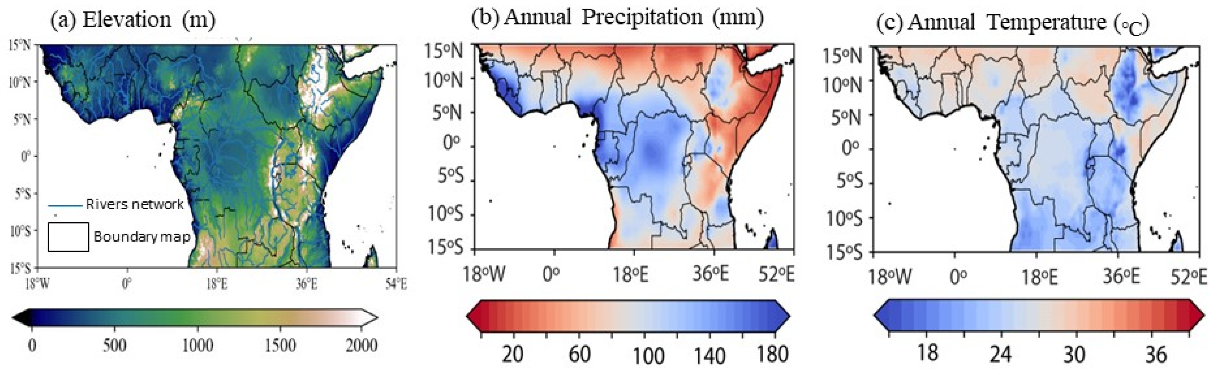
2.1. Study Area Description

Equatorial Africa is located between 15°00′00″N and 15°00′00′′S and 18°00′00″W and 54°00′00″E (Figure 1). The EQA region straddles the equator in equal halves. The upper half lies in the Northern Hemisphere, and the lower half falls in the Southern Hemisphere. The Atlantic Ocean is located to the west, and the Indian Ocean is located to the east. The EQA falls under the sub-regional blocs, namely, West Africa (WAF) in 20°W–20°E, 0°–28°N [42,43,44], East Africa (EAF: 34°–42°E, 5°S–5°N [45,46,47]), and Central Africa (CEF: 5°–35°E, 15°S–15°N [48,49,50]) as defined in [51].
The WAF experiences the West African Monsoon (WAM), and the EAF experiences the East African Monsoon (EAMS), characterized by convective precipitation and high temperatures. The CEF experiences both WAMs and EASMs depending on the seasonal movement of the intercontinental tropical convergence zone (ITCZ) [52].
Their climate follows the four seasons: summer (June–August), autumn (September–November), winter (December–February), and spring (March–May). Late spring, summer, and autumn are the longest and shortest rainy seasons for NH and are usually convective for WAF and EAF. At the same time, the CAF experiences a tri-modal rainfall pattern in locations near the equator [48,53].
The region’s climate has regulated a variety of complex extents of geographical features with highlands (e.g., Ethiopian, Kenyan, and Cameroonian Highlands) [52] (Figure 1a). The highest elevation, which is >5000 m, is Mount Kilimanjaro in Tanzania. The lowlands are located in the WAF regions (Figure 1a). The lowlands and rivers define the region’s hydrology. Huge water bodies (e.g., Lake Victoria) and large rivers (e.g., the White and Blue Nile Rivers) are located in EQA and host a variety of watersheds, such as the Congo Basin, Volta, Chad, etc.
Teleconnections, such as the global sea surface temperature (SST) and regional atmospheric circulations, are reported to shape the region’s climate [54,55,56,57,58].
The computed annual and seasonal climatology values based on the datasets described in Section 2.2 during 1980–2020 are listed in Table 1. The average annual precipitation is 89 mm and varies across seasons in the range between 77 mm (summer) and 98 mm (winter) (Table 1; Figure 1b). The average annual temperature is 25 °C, with the warmest season found to be the spring and the coolest seasons recorded in autumn and winter, respectively (Table 1; Figure 1c).

2.2. Dataset Description

We used 40 years (1980–2020) of monthly datasets of GLEAM products and climatic parameters (e.g., air temperature, precipitation, wind speed (surface and 850 hPa), relative humidity), and hydrological variables (soil moisture), as well as global SST.

2.2.1. Satellite-Based Products

We downloaded long-term satellite-based evapotranspiration (PET and AET), and soil moisture data (root zone) from the GLEAM (Version 3.3a) website for the period 1980–2020 (https://www.gleam.eu/ accessed on 22 January 2023). The gridded datasets were obtained at 0.25° × 0.25°. Readers are referred to documentation on GLEAM’s development and production [15,16,59]. The data has been widely validated in many studies [22,23,60].
λ P E T = ϕ Δ Δ + γ ( R n e t G )  
where λ represents the latent vaporization (MJ kg−1), Δ represents slope of the saturated water vapor-temperature curve (kPaK−1), γ represents psychometric constant (kPaK−1), ϕ is the Pristley and Taylor coefficient, R n e t denotes net radiation (Wm−2), and G denotes soil heat flux (Wm−2). G is computed as a function of Rnet and land cover. Refer to [16] for details on Rnet, G, and landcover information. Based on guidelines, each Priestley and Taylor [61] value corresponds to a specific land cover type. In [16], PET was estimated to be achieved by converting into AET, and its components (e.g., transpiration, interception, bare soil, etc.) are based on land cover information and other relevant information based on a formulation made by Priestley and Taylor [61].

2.2.2. Reanalysis-Based Products

We used the latest land-monthly ERA5 datasets downloaded from the European Centre for Medium-Range Weather Forecasts ((ECMWF) (ERA-5 hereafter)) website [62] (accessed on 20 April 2023). The climate variables obtained are surface wind speed (WS) and relative humidity (RH). In addition, wind speed at 850 hPa was obtained to conduct regional atmospheric circulation analysis. The daily gridded climate data were obtained at a daily scale and spatial resolution of 0.25° × 0.25° for 1980–2020. Details on this dataset are found in [63,64,65,66,67,68,69].

2.2.3. Gauge-Based Gridded Products

In addition, monthly precipitation and air temperature data were obtained from the CRU (Climatic Research Unit) website [70] (accessed on 20 March 2023) at a spatial resolution of 0.5° × 0.5° from January 1980 to December 2020. Readers are directed to [43] for more information. This dataset has been widely used in past studies [71,72].

2.2.4. Auxiliary Data Products

Also, we obtained the mean global SST dataset at a horizontal resolution of 1.0° × 1.0°. The data is produced by the GHRSST Global Data Assembly Center (GDAC) at the Jet Propulsion Laboratory (JPL) Physical Oceanography Distributed Active Archive Center (PO. DAAC). The monthly data was downloaded from http://ghrsst.jpl.nasa.gov/GHRSST_product_table.html [73] (accessed on 20 January 2023).
We computed the climatology of the long-term parameters using spatial and temporal averaging over the period 1980–2020. The datasets were computed using Climate Data Operator (CDO, version 1.6.4). All the datasets were converted to a spatial resolution of 0.25° × 0.25° using bilinear interpolation [46,47]. Annuals and seasons are used as the units of analysis. Based on past studies, several evaluation studies have shown that the use of these datasets is reasonably consistent with ground-based datasets [16,63,64,71,74,75]. The choice to use particular data was due to its utility and quality for the study. In the study area, CRU, as a gauge, is known to best match the precipitation and temperature patterns due to the extensive use of weather stations. With regard to other climatic variables (ET, wind speed, and relative humidity), the use of satellite-observed ET and ERA5 reanalysis is best suited for the study area due to the limited or lack of station-based measurements in the region [15,63].

2.3. Methods

2.3.1. Linear Trends

The non-parametric Mann-Kendall (MK) [76,77] was used to compute the trend analysis, and the Theil-Sen slope [78,79] was used to estimate the slope of the trends. These two non-parameter tests are preferred as they can handle outliers in datasets. The World Meteorological Organization (WMO) recommended its use for such analysis [48]. In Equations (2)–(4), we present the formula for computing the linear trends. When S is positive, the trend is increasing, whereas a negative value shows the trend is decreasing. The MK trend test is carried out by calculating the S statistic as:
S = i = 1 n 1 j = i + 1 n sgn ( x j x i )
where S is the rating score (called the Mann-Kendall sum), n is the number of observations, x i and x j are the ith and jth observations, and sign () is the sign function, which can be calculated as:
sgn ( x i x j ) = { 1 ,       if   ( x j x i ) > 0 0 ,         if   ( x j x i ) = 0 1 ,       if   ( x j x i ) < 0
We compute the variance based on Equation (2):
v a r   ( S ) = n ( n 1 ( 2 n + 5 ) i m t i ( t i 1 ) ( 2 t i + 5 ) 18
where m is the number of groups with tied ranks, each with t i tied observations. Since MK is designed by standardized Z, computed as:
Z s = { S 1 v a r ( s ) , i f   S > 0 0 ,                           i f   S = 0 S 1 v a r ( s ) ,       i f   S < 0
where no trend exists if − Z α / 2 Z Z α / 2 at significance level ( α ), otherwise trend exists at significance level ( α ).
The Theil-Sen slope [78,79] of n pairs of data points was computed based on:
Δ σ = median ( x j x i j i )
where Δ σ denotes the slope in two data time series, data values ( x j , x i ) for j as well as k (j > k). When Δ σ > 0 and Δ σ < 0 denote increasing and decreasing trends, respectively.
Also conducted linear regression analyses (Equation (5)) at annual and seasonal scales after the trend’s slopes were computed. Note that the original data series were used to derive the trend slope equation below.
y t = β t × X t
where y t denotes the data value obtained from the slope equation; Xt represents the intercept; and t is the time.

2.3.2. Break Detection Using a Bayesian Test

We adopted the Bayesian method due to its ease of use to examine the abrupt changes based on the mean values; more information on this technique is found in [80,81]. This method has lately received significant attention in eco-hydrological studies [82,83,84,85].

2.3.3. Standardized Anomalies

The climate dataset was standardized using the formula below.
z std = z i z ¯ σ
where z s t d is the standardized z, z ¯ is the average, and σ is the standard deviation of the variable S.
Pearson correlation coefficients ( R x y ) between the ET (X) and the climatic parameters (Y) are computed as follows:
R x y = i = 1 n ( X i X ¯ ) ( Y i Y ¯ ) i = 1 n ( X i X ¯ ) 2 i = 1 n ( Y i Y ¯ ) 2 2
where R x y is the correlation coefficient between parameters X and Y; X i is the ET value of the time i (mm); Y i is the value of the hydroclimatic factor in the time I; and X ¯ and Y ¯ are the averages of ET and hydroclimatic factor, respectively.

3. Results

3.1. Interannual and Seasonal Variations in ET

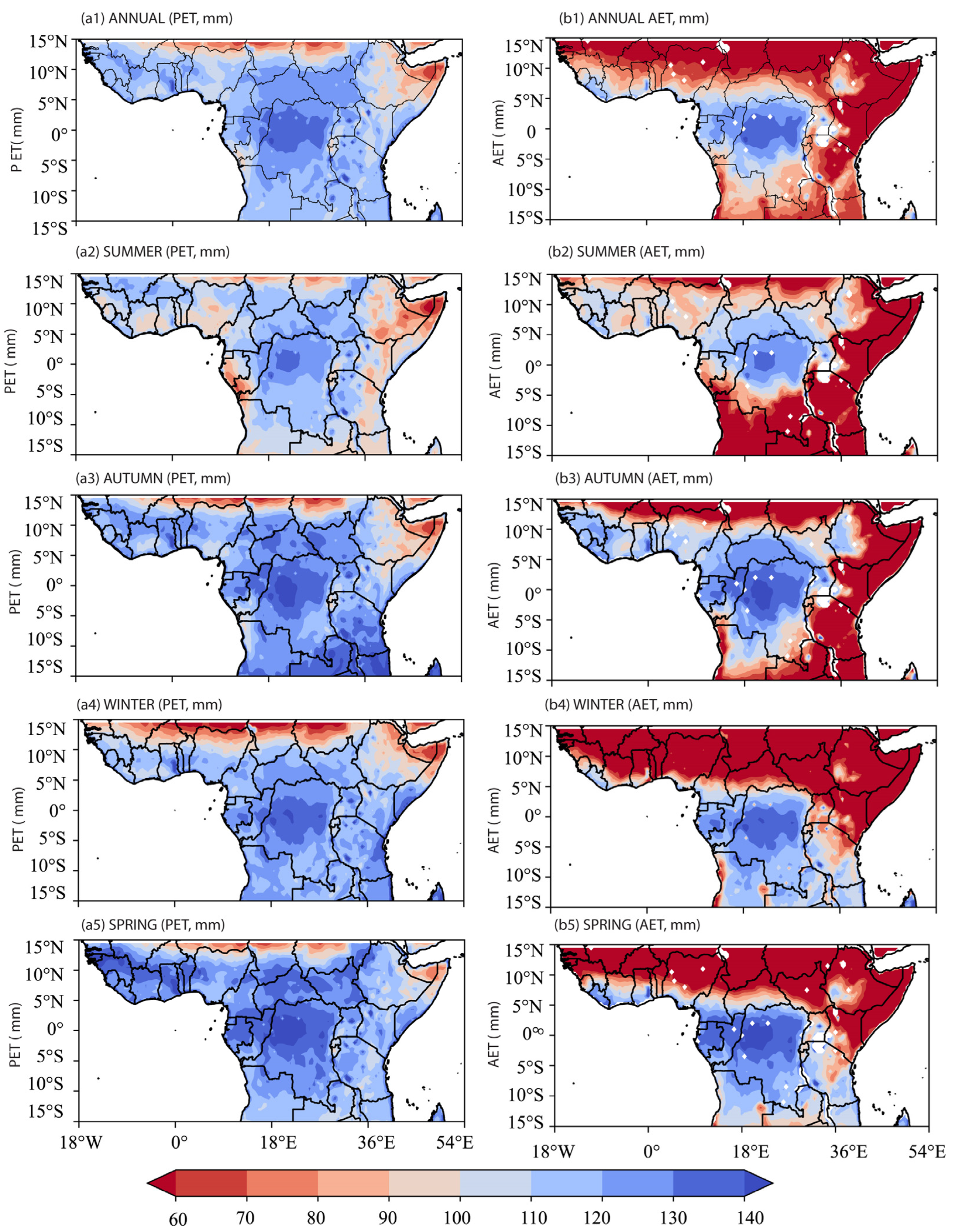
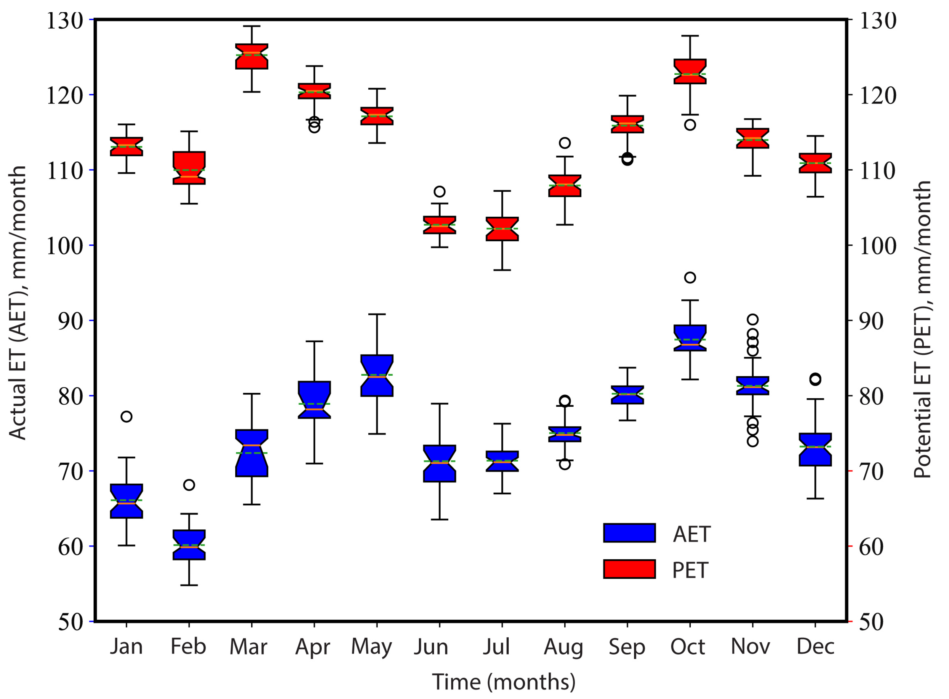
3.1.1. Seasonal Variability in PET and AET

Figure 2 presents the spatial patterns of the climatological annual PET (a1) and AET (b1) and the climatological seasonal PET (a2–a5) and AET (b2–b5) averaged over the 40-year EQA. Overall, a distinct spatial variability in both PET and AET over different regions is noticeable. The annual and seasonal amounts showed a latitudinal gradient (Figure 3). The annual PET values range from 80–≥140 mm, while the AET values range 50–≥90 mm from 1980 to 2020 (Figure 2(a1,b1)). This result is consistent with past studies [86]. The annual PET result in this study is consistent with [87] in Canada (PET = 100 mm) during 1979–2016. Furthermore, our result was consistent with [10], which found a national mean value of 256 mm. Ref. [88] found an annual amount of 239 (100–600 mm yr−1) from 1979–2008.
The amount of ET for the different seasons is shown for PET (AET) in Figure 2(a2–a5) (Figure 2(b2–b5)). Boreal spring and autumn values show higher amounts at 110–128 (50–≥85 and 109–125 (72–≥85) mm, whereas low amounts are shown in boreal summer 110–114 (70–85 mm) and winter 108 110 (58–78 mm). The seasonal values are consistent [10]. Ref. [88] found a summer value of about 390 mm (i.e., 65% of 600 mm yr−1) and below 10 mm month−1 in winter. In terms of ET distribution, humid regions in the 15–25°E and 5°S–5°N show similar amounts. The PET and AET values in the Congo Basin are close to each other (PET/AET > 100 mm), consistent with the complementary relationship hypothesis [34], and similar results are widely reported in past literature [33]. This is consistent with humid areas [89]. Huge interannual and seasonality variability differences are shown in arid and semi-arid climates at 8–15°N in NH and 25–30°S in SH. A similar result is presented at 26–52°E and 10°S–5°N, consistent with a semi-arid region [90,91].
Figure 3 presents the annual PET and AET climatology cycles from 1980 to 2020, respectively. The temporal distribution ranges from 100 to 125 mm. PET ranges from 100–130 mm, and AET ranges from 50–90 mm. Generally, two peaks are shown in PET (in March and October), whereas AET peaks in May and October. Low PET values (100 mm) occurred in July (Figure 3, red color). Low AET values occurred in February (Figure 3, red color). The remaining seasons showed similar trends despite differences in magnitude (Figure 3).

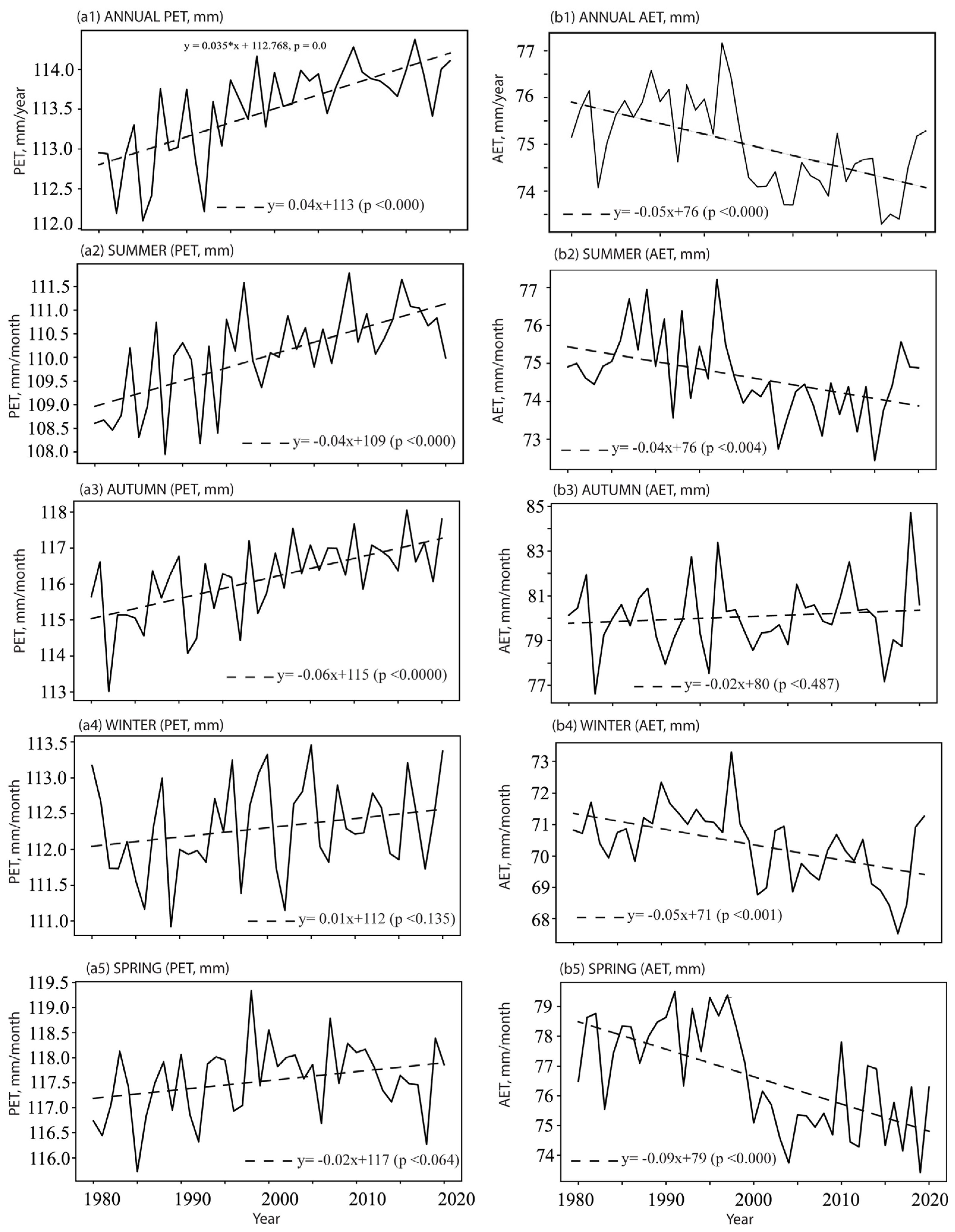
3.1.2. Long-Term Changes in PET and AET

Figure 4 presents the variations of long-term linear trends averaged over 40 years at annual and seasonal timescales. The interannual trends show an increasing trend at 0.035 mm yr−1, whereas AET shows a decreasing trend at 0.05 mm yr−1. The PET mean (range) is 113 mm yr−1 (112–114 mm) (Figure 4(a1)). AET is 75.5 mm yr−1 (range of 72–77 mm) (Figure 4(b1)).
The seasonal trends in PET (a2–a5) and AET (b2–b5) were quantified. The temporal trends showed the opposite direction, but the magnitude varied. The summer PET (AET) shows an upward (downward) trend at the same rate of 0.04 mm yr−1. Boreal summer PET mean (range) values were 109.75 mm (108–111.5 mm) and an AET value of 75 mm (72–77 mm) (Figure 4(a2,b2)). The remaining seasons were as follows: autumn PET (AET) increased (decreased) at a rate of 0.06 (−0.02) mm yr−1 (Figure 4(a3,b3)). Winter PET (AET) increased (decreased) at a rate of increasing 0.01 (−0.05) mm yr−1 whereas spring PET (AET) increased (decreased) at a rate of increasing 0.02 (−0.09) mm yr−1 (Figure 4(a4,a5,b4,b5)).
Figure 5 illustrates the spatial trends computed at pixel level at annual (a1,b1) and seasonal scales (a2–a5,b2–b5). The spatial trends showed opposite trends in PET and AET. These results suggest that the locations with upward PET trends inconstant with AET trends showed downward trends in the same location, consistent with [33,34] and related to the opposite feedback mechanism between PET and AET [34].
The spatial trend showed significantly increased (or decreased) PET (AET) trends at a rate range of 0.8 (−0.8 mm). This result of decreasing AET over the region is consistent with [39,85,92] and complements increasing PET according to [34]. However, humid climate zones in Figure 5(a1,b1) showed a declining trend in wetter environments at 15°–25°E and 5°S–5°N (i.e., Congo Basin), which is not surprising in wetter environments where PET and AET are nearly equal [33]. Our result is consistent with the results reported in [87]. In contrast, semi-arid and arid conditions provide opposite directions for PET and AET. The increasing trend in the East Sahel (0°–10°E, 5°–15°N), northwest of Kenya, the Horn of Africa region, and the periphery of the Guinea Coast is moving downwards along the edges of the Atlantic Ocean.
Moreover, the seasonal analysis is presented in Figure 5(a2–a5,b2–b5). The summer and spring seasons showed a PET (AET) increase (or decrease) at a rate of 0.4 (0.7) mm. Both autumn and winter presented similar trends in PET (AET) magnitude but opposite directions, a rate of 0.6 mm (Figure 5(a3,a4,b3,b4)). The results of an increase in PET and a decrease in AET, and vice versa, are consistent with two conditions that allow AET to fall below PET [34]. According to literature, as reported in [93,94,95], this occurs under conditions where limited moisture is available and excess energy warms the dried atmosphere. Many studies have reported on the analysis of PET and AET variability annually and seasonally in different regions [7,93], consistent with the complementary relationship hypothesis [33].

3.1.3. Detecting Abrupt Changes in PET and AET

Figure 6 presents the detection of an abrupt change in the mean annual PET and AET time series from 1980 to 2020. The Bayesian test was used to detect breaks, and the results show a difference in the change point for PET (Figure 6a) and AET (Figure 6b). The PET abrupt change point occurred in 1995, whereas the AET abrupt change point occurred in 2000. This is consistent with [84]. In [85], the PET abrupt change point occurred in 1993 and 2003.

3.2. Drivers of Interannual and Seasonal Variations in PET and AET

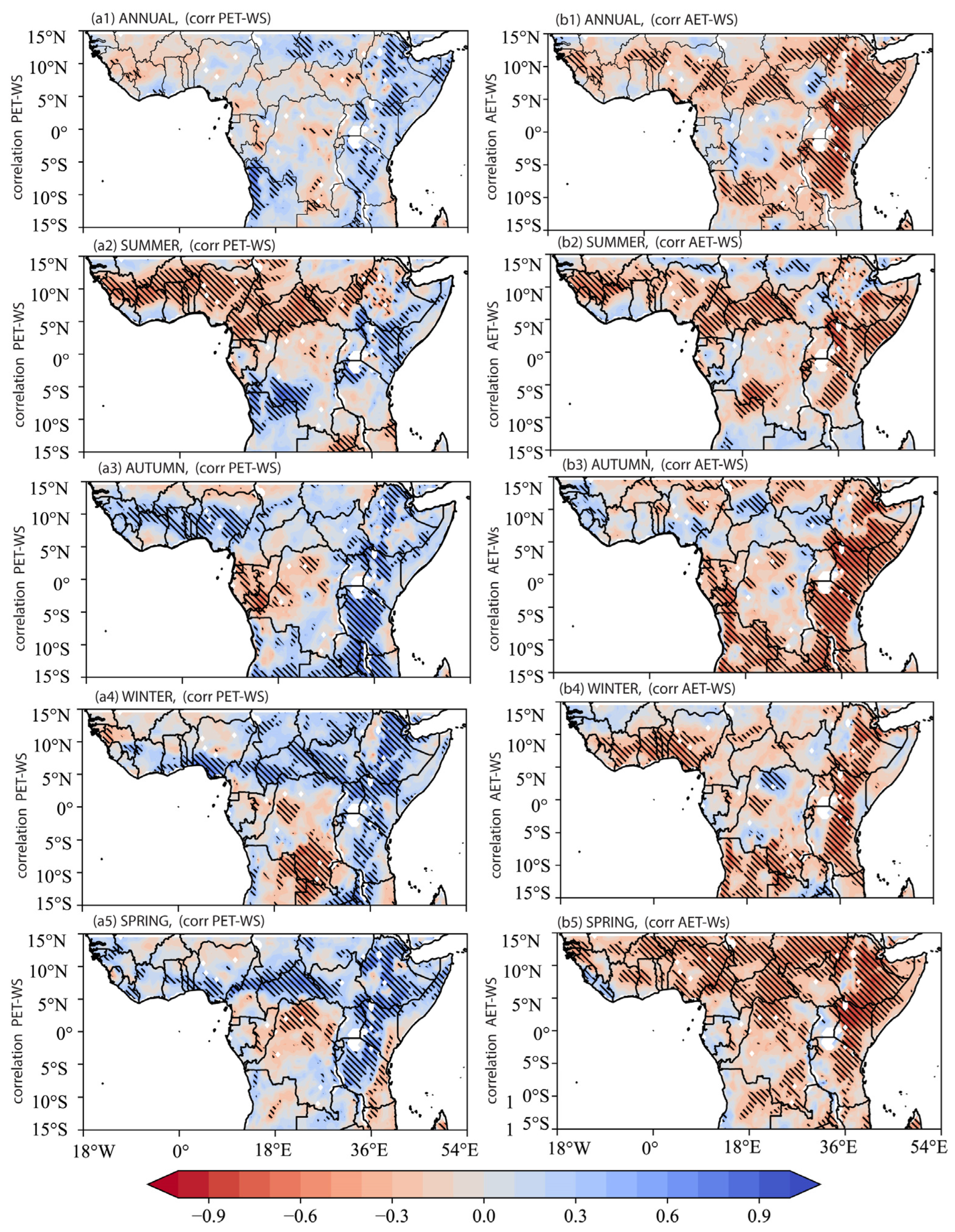
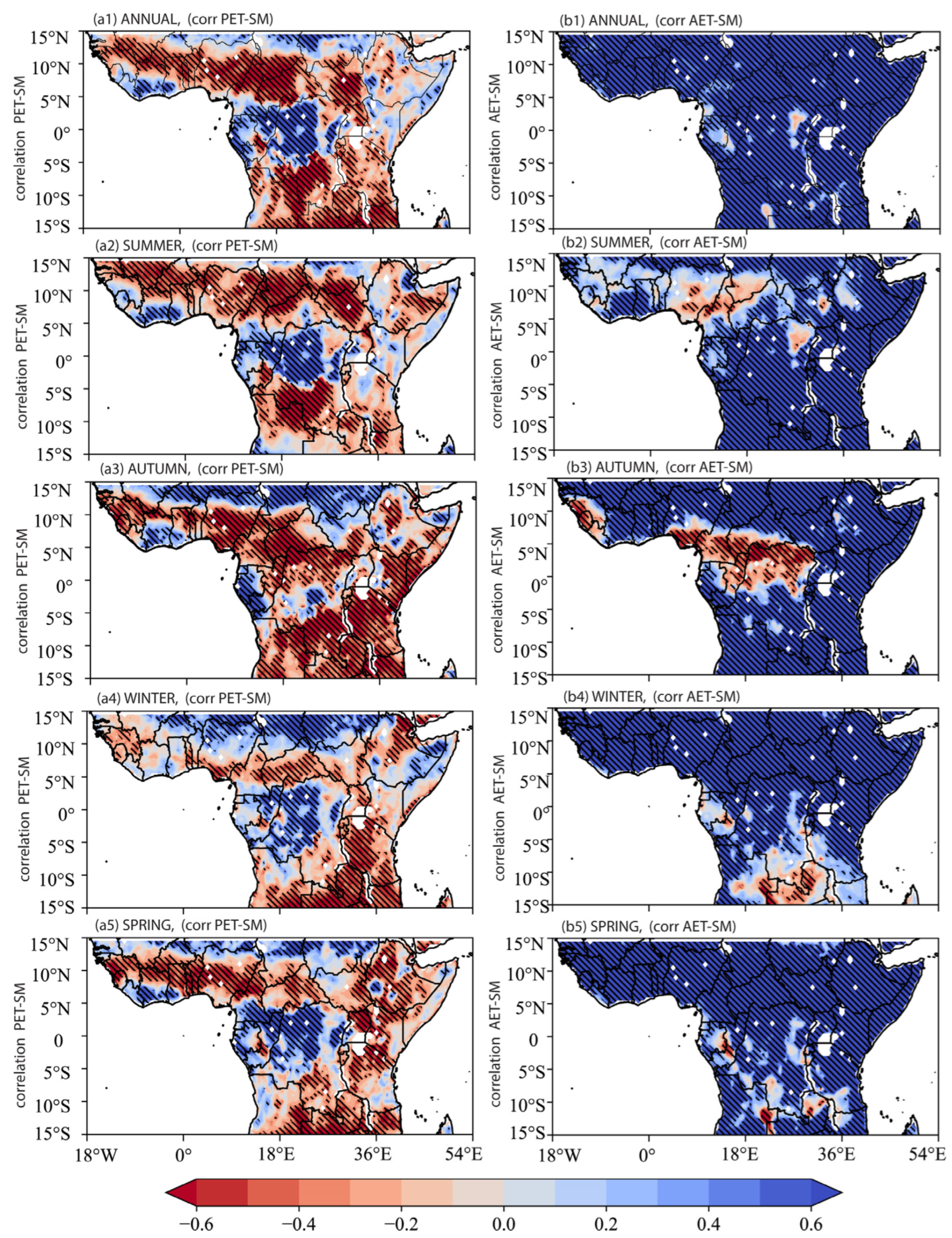
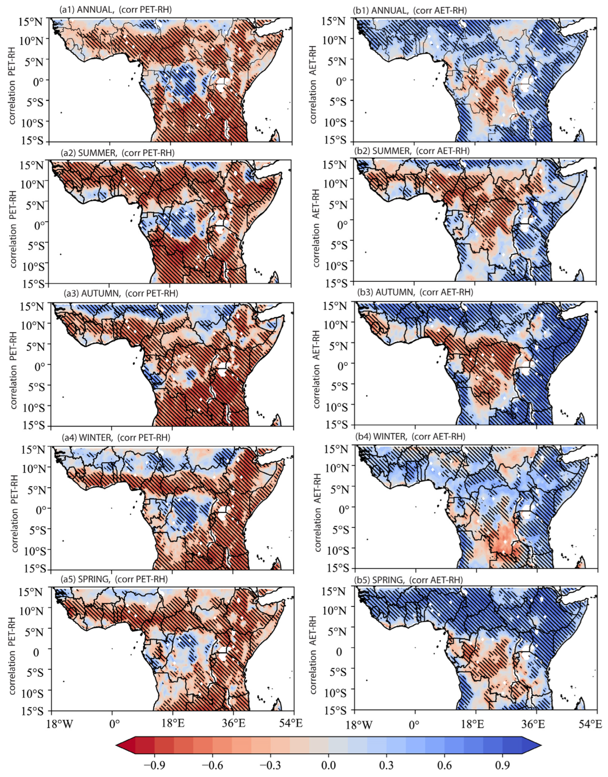
3.2.1. Spatial Correlation Maps

Figure 7 presents the spatial correlation between precipitation (PREC) and PET/AET. There are differences in the spatial characteristics of the correlations between PET/AET and PREC in semi-arid and arid conditions, whereas humid conditions showed identical correlation patterns. The PREC link with PET/AET, mostly in humid conditions at 15°–25°E, 5°S–5°N (Congo Basin), revealed a negative correlation. However, in arid/semi-arid conditions, positive relationships exist in the Sahelian belt (18°W–54°E, 10°–15°N), the peripherals of the Guinea Coast (18°W–15°E), the northern hemisphere (NH) (0°–5°N), and the southern hemisphere (SH) (5°S–0°) (Figure 7(a1,b1)). Moreover, the correlation analysis of PET/AET and four climatic variables was performed at seasonal scales (Figure 7(a2–a5,b2–b5)). Huge differences in spatial characteristics of correlation between PET and PREC vs. AET and PREC were observed in 5°S–5°N (Congo Basin) and the entire locations in 26–52°E, 10°S–5°N, and 15°–5°S (Figure 7(a2–a5,b2–b5))—the seasonal correlation range from −0.9 to +0.9. The result presented a bipolar spatial pattern of the correlations between PET and PREC vs. AET and PREC (Figure 7(a2,a3,b2,b3)): weaker in geographic locations 5°S–5°N (Congo Basin) but stronger (−0.5 ≤ r ≥ −0.9) in geographic locations 26–52°E, 10°S–5°N, and 15°–5°S.
However, in the same period and at the same time, negative values are distinctively located in 10°–15°N (the Sudano-Sahelian belt) and 15°S–5°S (the northern Kalahari Desert region). (Figure A1(a1,b1)). Seasonal results show the correlation analysis of PET/AET, and SM was performed at seasonal scales (Figure A1(a2–a5,b2–b5)). Seasonal analysis revealed an interesting contrast in spatial correlation in the 5°S–5°N (Congo Basin), where except for boreal autumn, positive values are observed between SM and PET (Figure A1(a2,a4,a5)) vs. SM and AET (Figure A1(a2,a4,b5)). The similar negative correlation values in autumn in the 5°S–5°N (Congo Basin) are interesting (Figure A1(a3,b3)). This result is consistent with water availability in regions controlled by SM-atmosphere feedback.
Figure 8 presents the spatial correlation between air temperature and PET/AET. Results showed correlation coefficient values ranging from −0.9 to +0.9. Overall, there is an opposite correlation pattern between PET and temperature (TEMP) vs. AET and TEMP in 5°S–5°N (Congo Basin) and 36°–54°E, 15°S–15°N (Figure 8(a1–a5,b1–b5)). Few exceptions in pocket locations in NH (0°–5°N) and SH (5°S–0°). Seasonal analysis revealed differences in the spatial characteristics of the correlations between PET and TEMP (Figure 8(a2–a5)) vs. AET and TEMP (Figure 8(b2–b5)). Distinctively opposite signs but strong correlations were observed in 5°S–5°N (Congo Basin), 10°–15°N (central Sahelian belt), and 36°–54°E, 15°S–15°N (Figure 8(a2–a5,b2–b5)). This result is consistent with [30] on PET and air temperature in Malaysia. In other past studies, TEMP had a strong relationship with PET and AET [7]. Ref. [96] reported a PET link with TEMP. Ref. [86] found PET declining with increasing TEMP.
The spatial correlation pattern displayed the opposite result for the same period and time (Figure A2). The negative PET/relative humidity (RH) correlation was similar in magnitude (−0.3 ≤ r ≥ −0.9), whereas positive AET/RH had the strongest correlations observed (0.4 ≤ r ≥ 0.9). Seasonal analysis showed opposite signs of correlation between RH and PET (Figure A2(a2,a4,a5)) vs. RH and AET (Figure A2(a2,a4,b5)). Our results are consistent with RH regimes’ effects on PET [96]. Ref. [7] RH regulations strongly link AET and PET with global warming [97]. The TEMP and RH of land-atmosphere feedback result in a strong connection between PET and AET [7].
Figure 9 illustrates the correlation analysis results between wind speed (WS) and PET vs. wind speed and AET. The PET/WS relative showed a heterogenous positive and negative correlation (Figure 9(a1)). The negative correlation between AET and WS shows a homogenous pattern (Figure 9(b1)).
The seasonal analysis is presented in Figure 9(a2–a5,b2–b5). Overall, the spatial pattern of the correlations between PET and WS vs. AET and WS varied across seasons. Both positive and negative correlations in PET/WS have been noticed in 10°–15°N and pockets in 15°S–5°S (Figure 9(b2–b5)). At the same location, AET/WS were negative (Figure 9(b2–b5)). In general, the similarity in correlation pattern in humid areas and the difference in correlation pattern in semi-arid/arid areas are consistent with the feedback mechanism between PET and WS vs. AET and WS in different climate zones [30,86,96]. Our results are consistent with [30] on PET and wind speed in Malaysia. The results are consistent with [86], which showed declining PET with decreasing wind speed. Other studies observed different regions and showed that decreasing trends in PET coincided with decreasing trends in surface winds [96].

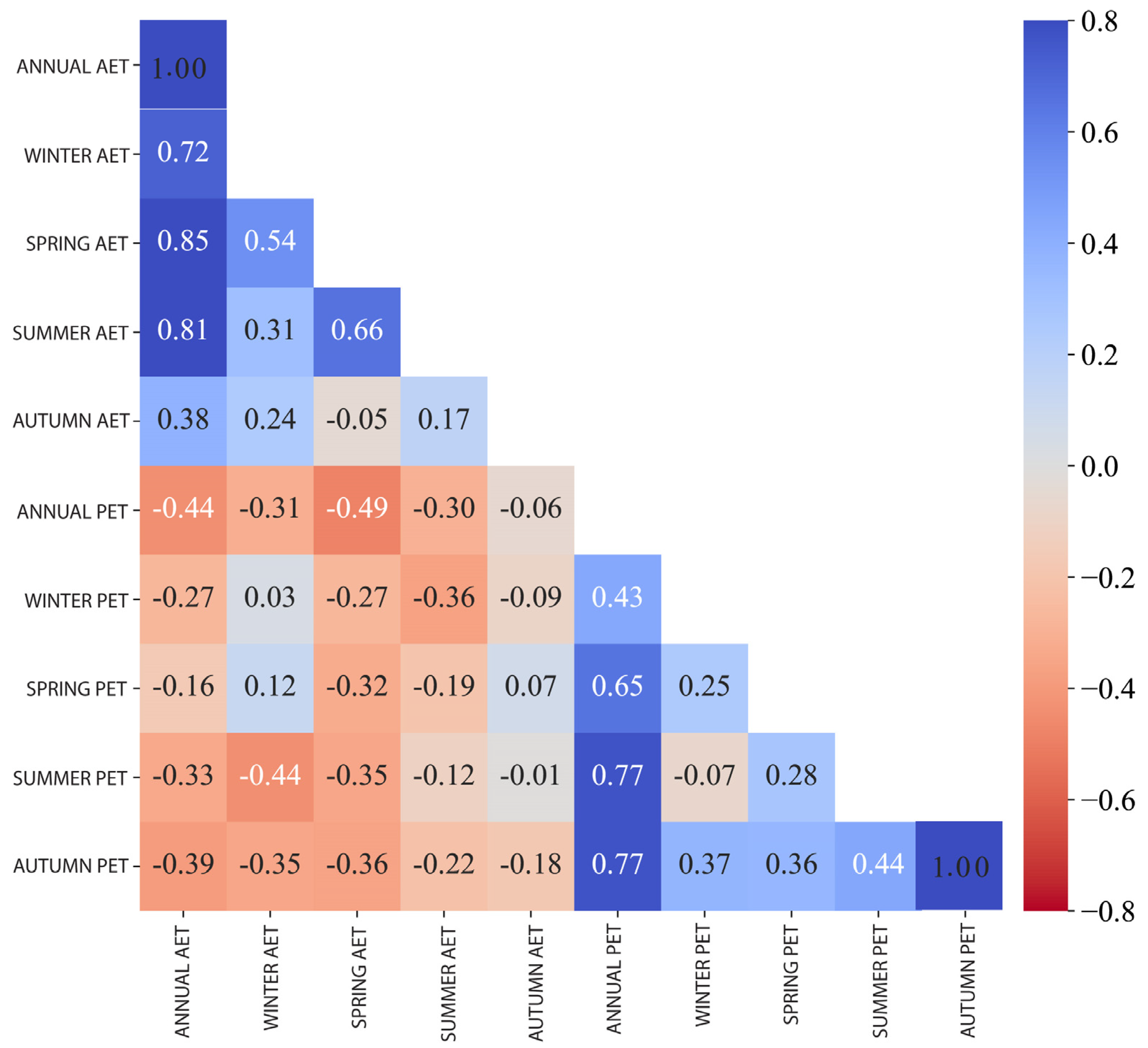
3.2.2. Temporal Correlation

Table 2 presents the temporal dynamics of potential evapotranspiration (PET), actual evapotranspiration (AET), and five climatic parameters based on annual values. Overall, the correlation coefficients varied in magnitude and sign of direction to reveal opposite PET and AET dynamics with climatic factors. A stronger (or weaker) relationship indicates a limiting (or not-limiting) driver of PET/AET variations. Overall, Table 2 reveals that air temperature, soil moisture, and relative humidity are limiting factors that explain the PET/AET temporal dynamics better than precipitation (PREC) and wind speed (WS).
SM presented a significant positive correlation coefficient (R) with PET (R < −0.68) and AET (R < 0.86), respectively, which is consistent with [98]. PREC presents a positive correlation with PET (R < 0.06) and AET (R < 0.25) but a weak relationship. The weak relationship is consistent with [23]. TEMP and RH had significant positive and negative correlation coefficients (R) with PET and AET. The stronger correlation between PET and AET showed opposite signs. PET/TEMP is 0.78, AET/TEMP is −0.58, PET/RH is −0.81, and AET/RH is 0.70, respectively. The signs of TEMP/RH with PET and AET are opposite. Increasing temperatures and declining precipitation are reported in the region [48].
The correlation analysis of the PET/AET with TEMP, RH, and SM suggests these parameters are considerably stronger, suggesting that they are limiting drivers of ET variations in the study area. The correlation strength between TEMP/ET is consistent with [99]. However, a weak relationship between PREC and PET (R < 0.23) and AET (R < 0.06), as well as WS with PET (R < 0.33) and AET (R < 0.40), suggests PREC/WS are not limiting factors. This result in Figure 10 compares the temporal coefficients. The magnitude and sign of the correlation analysis are complementary [33], consistent with the analysis of PET and AET variability annually and seasonally in different regions [7,93].

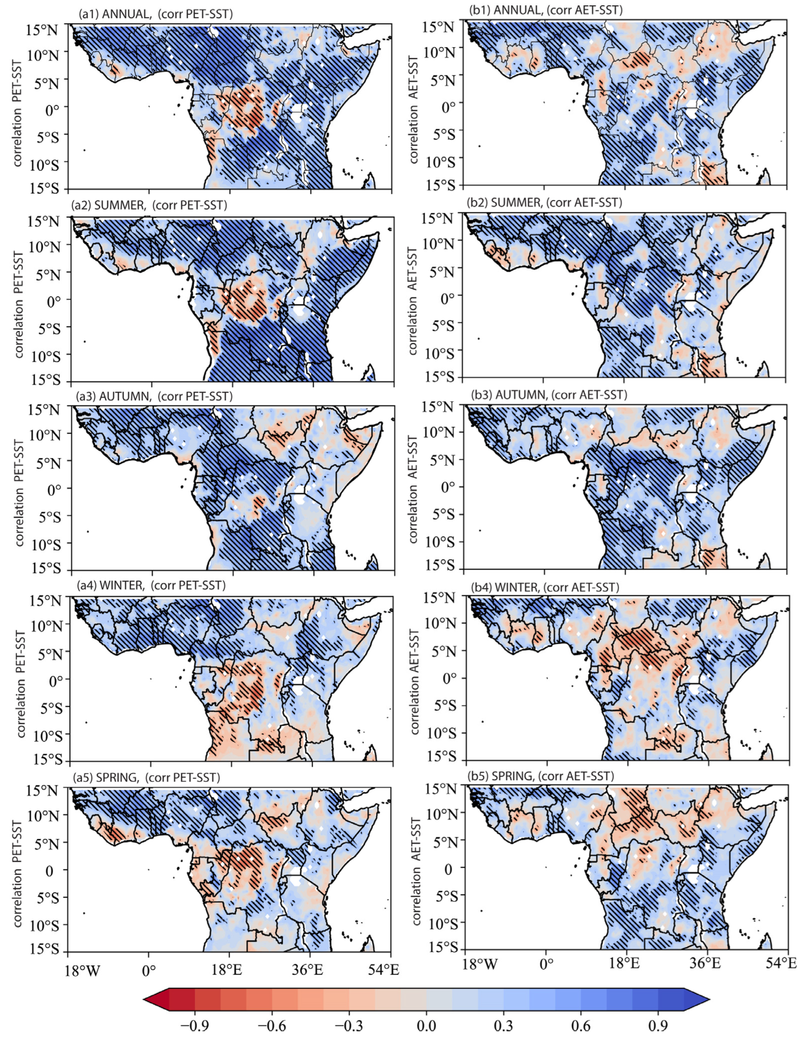
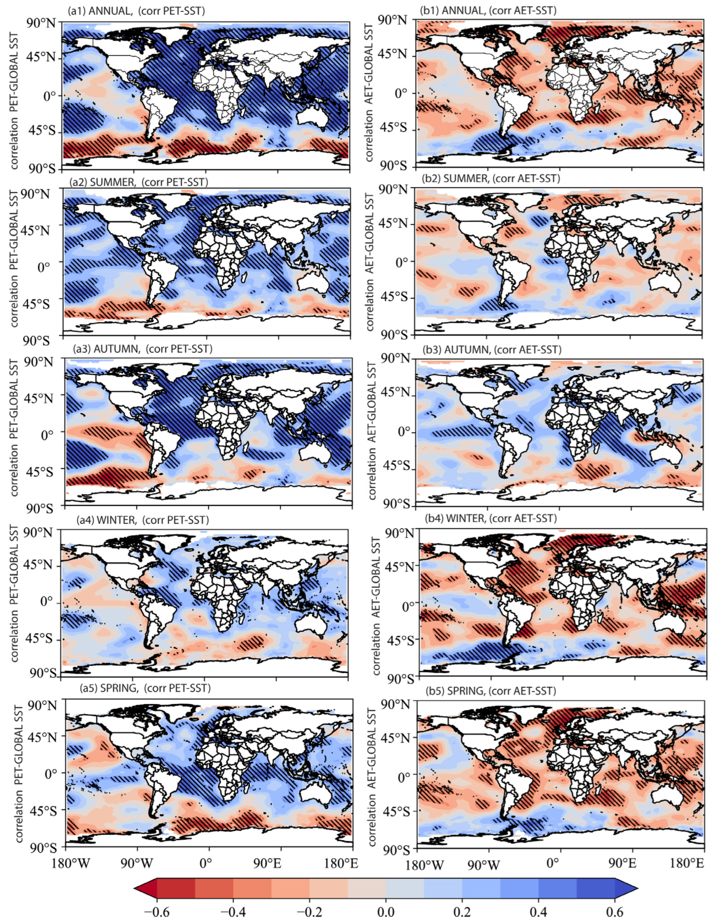
3.2.3. Relationship between PET/AET and Global SST

Figure 11 shows the correlation analysis performed between PET and SST anomalies and AET and SST anomalies at annual and seasonal scales. We observed that SST anomalies have a significantly positive correlation with PET (Figure 11(a1)) and AET (Figure 11(b1)) in the study, except for the opposite correlation observed in 5°S–5°N (Congo Basin) and pockets in 15°S–5°S (in the bottom right) (Figure 11(a1,b1)). Correlation analysis was performed between the evapotranspiration (PET and AET) and the SST anomalies for the summer (Figure 11(a2,b2)), autumn (Figure 11(a3,b3)), winter (Figure 11(a4,b4)), and spring (Figure 11(a5,b5)) seasons from 1980–2020. In boreal summer, we observed that SST anomalies have a significantly positive correlation with PET (Figure 11(a2)) and an opposite correlation with AET (Figure 11(b2)) in 5°S–5°N (Congo Basin) and 26–52°E, 15°S–5°N (EAF). Boreal autumn showed SST anomalies, with PET/AET showing a similar pattern of positive correlations in 18°W–18°E, 15°–15°N and negative correlations in most of the Sudano belt (5°–15°N) in Figure 11(a3,b3). Few exceptions show the difference in sign of spatial correlation was observed in pockets of 26–52°E, 15°S–5°N (EAF), and 15°S–5°S (in the bottom right) (Figure 11(a3,b3)). In boreal winter, we observe a heterogenous spatial pattern, with PET/SST anomalies showing an opposite correlation with AET/SST anomalies over most of the sub-divisions in India (except pockets of areas having similar correlation results (in magnitude and direction)) (Figure 11(a5,b5)).
The annual and seasonal PET and AET variability analysis is closely linked with global SST anomalies in the tropical Atlantic and Indian Oceans (Figure A3). It is more obvious, as there is homogeneity in the spatial correlation pattern and variations in the relationship between SST anomalies and PET (Figure A3(a1)) as well as SST anomalies and AET (Figure A3(b1)), respectively. Similar results are shown in the seasonal analysis (Figure A3(a2–a5,b2–b5)).

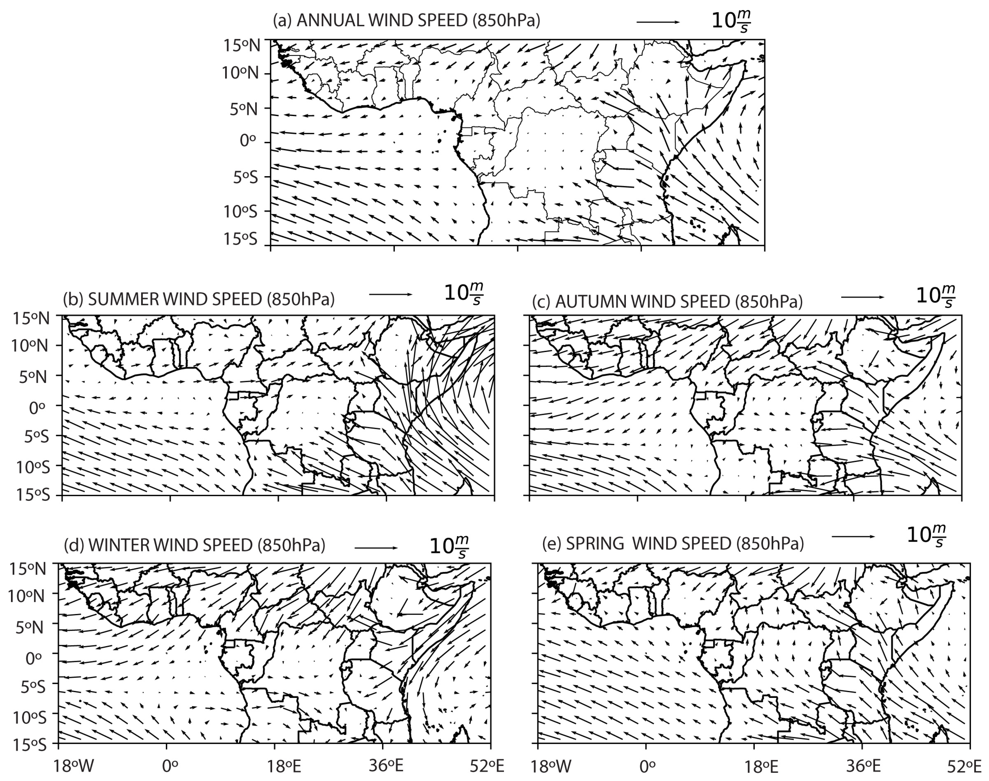
3.2.4. Relationship between PET/AET and Large-Scale Circulations

We present the regional wind circulation annually and during the different seasons over equatorial Africa (Figure 12). We observed two major wind directions, particularly the northward and southward winds. The northward is characterized by dry particles, while the southward, called monsoon wind circulation, transports moisture from the ocean. In the annual (Figure 12-Annual) and winter (Figure 12d) seasons, West Africa’s region is dominated by northward winds reaching a large ocean surface. However, a difference is noted between the confluence zone/region of the northern and southern winds. That is likely to indicate the ITCZ’s position.
The location of the confluence zone at the annual (Figure 12a), winter (Figure 12d), and autumn (Figure 12c) seasons indicates dominant dry wind circulations over the continental region, leading to weak moistening conditions. The eastern region experiences southeastern circulation during the annual (Figure 12a) and autumn (Figure 12c) seasons. Meanwhile, the eastern region experiences northeastern winds during the winter season. The moisture could be transported from the Indian Ocean into the eastern country, leading to favorable precipitation conditions. During the spring (Figure 12e) and summer (Figure 12a) seasons, most West African countries are influenced by the monsoon circulation, with strong wind circulation during the summer.

4. Discussion

Using a GLEAM remote sensing dataset from 1980 to 2020 across equatorial Africa, we investigated the spatiotemporal variations and trends of two types of ET (PET and AET) at different annual and seasonal scales. Moreover, the climatic, global SST, and large-scale factors that drive ET seasonality were examined.
During the 40 years, we quantified the seasonality of the two ET averaged across the study and revealed PET is 110 mm yr−1 (summer = 112 mm; autumn = 117 mm; winter = 109 mm; and spring = 119 mm) compared to the annual value of AET of 70 mm (summer = 78 mm; autumn = 79 mm; winter = 55 mm; spring = 78 mm). The averaged spatial PET (AET) tended to be higher in humid regions than in semi-arid/arid zones, consistent with past studies [86]. The mean annual PET (AET) values are consistent with those obtained for different regions of the world at annual scales [10,87,88] and seasons [10,88], and the result is consistent with the complementary relationship hypothesis by [34] and reported in [33,89,90,91].
Previous studies have examined the spatial pattern of PET and AET trends using various datasets, and the trends computed were based on the Mann-Kendall (MK) test and Sen’s analysis. These previous studies generated trend types for PET and AET: positive, negative, or no trend. A significant decrease in PET and an increase in AET and vice versa have been reported in different regions of the world, including China [33,84,85], Canada [88], Bangladesh [91], Brazil [90], and Pakistan [100]. With GLEAM data, the annual PET (AET) for the whole study area increased or decreased significantly from 1980 to 2020, with PET increasing at a rate of 0.035 (0.05) mm yr−1. Seasonal analysis reveals that the significant upward (or downward) trend is prominent during summer at the same rate of 0.04 mm yr−1, autumn PET (AET) increased (or decreased) at a rate of increasing 0.06 (−0.02) mm yr−1, winter PET (AET) increased (or decreased) at a rate of increasing 0.01 (−0.05) mm yr−1, whereas spring PET (AET) increased (or decreased) at a rate of increasing 0.02 (−0.09) mm yr−1. The decrease in AET is consistent with previous literature [92], whereas the increasing PET is consistent with the complementary relationship hypothesis by [34] and reported in [33,89,90,91].
Abrupt changes are a universally important part of the climate system, as the conditions can cause the climate pattern to change sharply [101,102]. The PET/AET linear trends may result in shifting trends in the region and differ spatially. Our results showed an abrupt change in trends in 1995 and 2000 for PET and AET, respectively. Interestingly, the different abrupt change times for PET and AET were based on an inverse peak trend abrupt change, where PET gradually increased from 1980–1994 but increased significantly from 1996–2020. AET gradually increased from 1980–1999 but decreased significantly from 2001–2020. The timing of abrupt changes in the ET is in line with that of heavy precipitation and temperature events during the study period. These findings suggest that changes in the frequency of extreme events (e.g., wet periods or dry periods) have a huge effect on mean ET. Our result is consistent with previous studies [84,85], where the reasons for the step changes varied across regions and were generally related to other climatic conditions and ecological factors. Further studies could explore the reasons for the different step changes in both PET and AET. Discerning the abrupt changes in the EQA regions could help explain the future causes and effects of historic variations in water resources and improve predictions of these parameters under climate change.
Next is the need to better understand and quantify the drivers, such as climatic factors, global SST, and regional atmospheric circulation patterns, of ET variability in a changing climate. Connecting the ET variation information to climatic and remote factors is a challenging task because the relationships are affected by many factors other than the ones listed. Previous studies have used the Pearson correlation to examine these relationships [30]. In general, ET is controlled by climatic factors (e.g., precipitation, air temperature, wind speed, relative humidity (RH)) and hydrological factors (e.g., soil moisture) [30,31]. In the literature, it is known that, according to the complementary relationship hypothesis, the spatial pattern of PET is closely linked to that of AET. First, PET located in wetter environments is equal to AET, whereas semi-arid or arid conditions have the opposite situation where PET exceeds AET and vice versa. Our analysis of the spatial and temporal dynamics of PET/AET across EQA with these climatic variables revealed results consistent with previous studies. The temporal dynamics revealed that air temperature, soil moisture (SM), and relative humidity (RH) are limiting factors. This suggests that increasing trends between PET and climatic factors showed decreases in AET and climatic variables consistent with [7,30,86,96,97].
Studies have shown a link between changes in ET variability and global SST and regional atmospheric circulation patterns through a complex of dynamics. However, the results are inconclusive. We analyzed this response based on PET/AET variability to understand this ocean-atmosphere feedback. The spatial pattern of the strength of this feedback is very strong and closely linked with global SST anomalies in the tropical Atlantic and Indian Oceans. The spatial correlation pattern is homogenous. The relationship shows identical magnitude but opposite signs at annual and seasonal scales. The result revealed two major wind directions, particularly the northward and southward winds, that influence ET interannual and seasonal variability. The possible connections between this ET seasonal-to-interannual variability and wind circulation were explored [78]. The wind circulation mechanism over the EQA plays a more vital role in how heat energy is transported into the region or vaporized moisture is removed from the region. Thus, increasing wind speed in the EQA blows water vapor in the air away to reduce humidity and increase the rate of ET, and vice versa, consistent with findings in [88,96].

5. Conclusions

This study investigated the seasonality, trends, and step changes in PET and AET and possible mechanisms of ET variability and changes based on regional atmospheric circulation patterns and global SST anomalies from 1980–2020. Based on the study’s analysis, the following results were concluded:
  • The annual and seasonal variability in PET (AET) varied in different climatic zones in the region. The annual PET values range 80–≥140 mm, while the AET values range 50–≥90 mm from 1980 to 2020. Seasonal PET (AET) values are presented as boreal spring 110–128 (70–≥85) mm and autumn 109–125 (72–≥85) mm. Low values are recorded in summer 110−114 (70–85 mm) and winter 108−110 (58–78 mm).
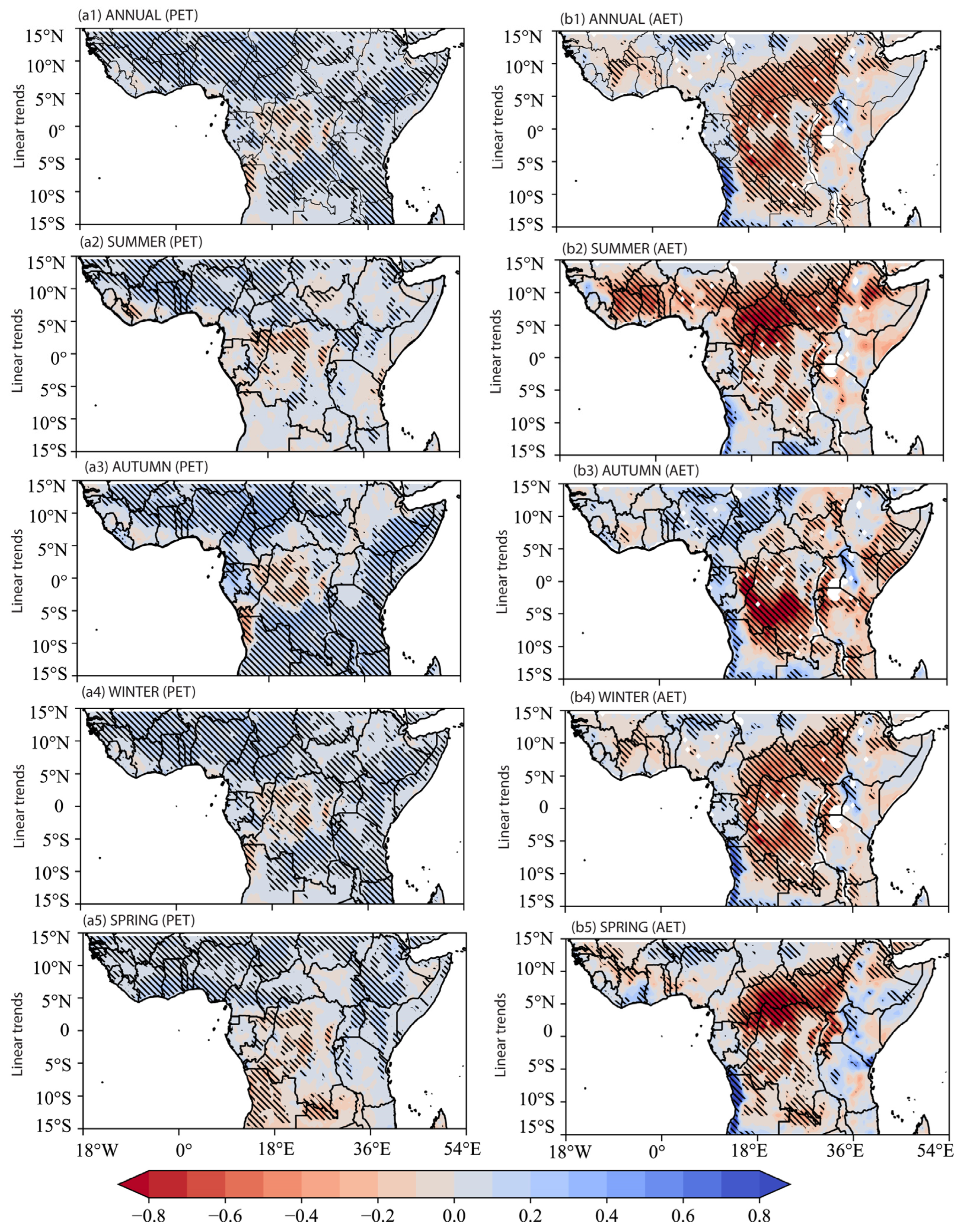
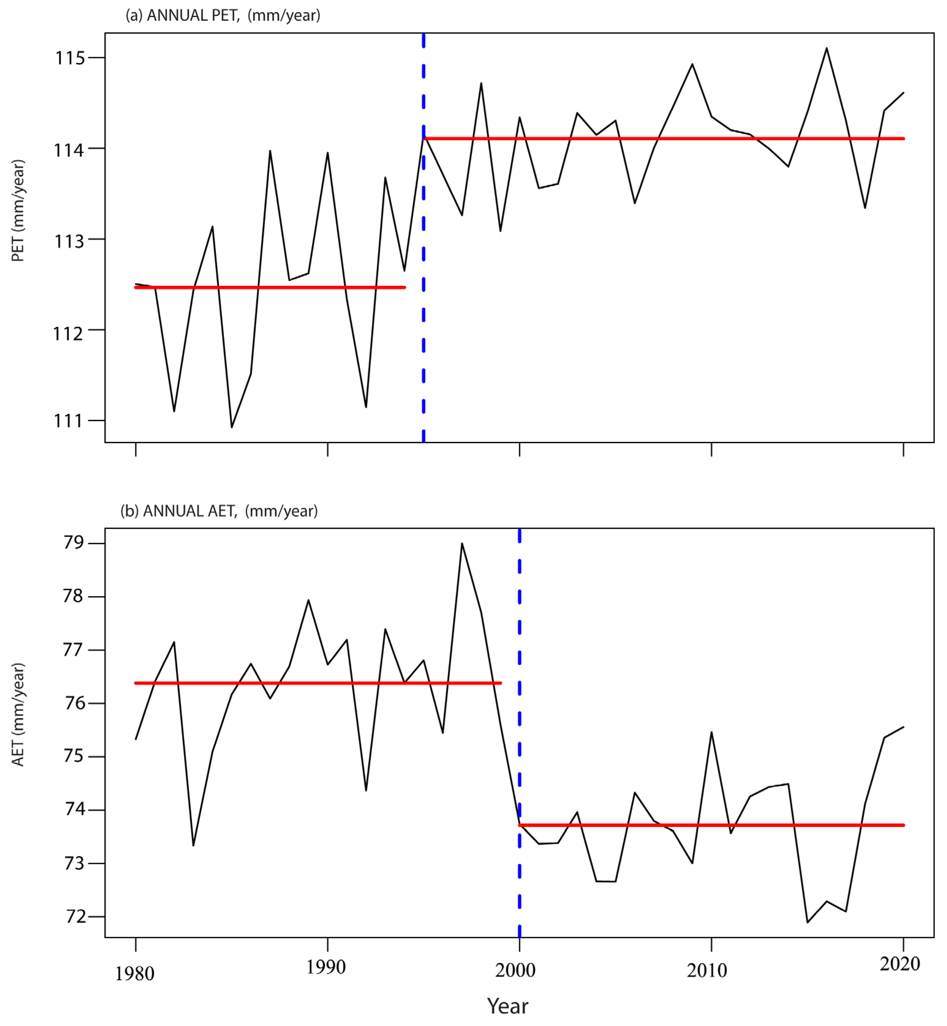
  • The interannual trends show an increasing (decreasing) trend at 0.035 (0.05) mm yr−1. PET mean (range) is 113 ((112–114) mm yr−1 and AET is 75.5 (72–77) mm yr−1. The PET (AET) seasonal trends were quantified over 40 years (1980–2020). The summer PET (AET) shows an upward (downward) trend at the same rate of 0.04 mm yr−1. The remaining seasons follow: autumn PET (AET) increased (decreased) at a rate of 0.06 (−0.02) mm yr−1. Winter PET (AET) increased (decreased) at a rate of 0.01 (−0.05) mm yr−1, whereas spring PET (AET) increased (decreased) at a rate of 0.02 (−0.09) mm yr−1. The PET abrupt change point occurred in 1995, whereas the AET abrupt change point occurred in 2000, based on the Bayesian test for change detection.
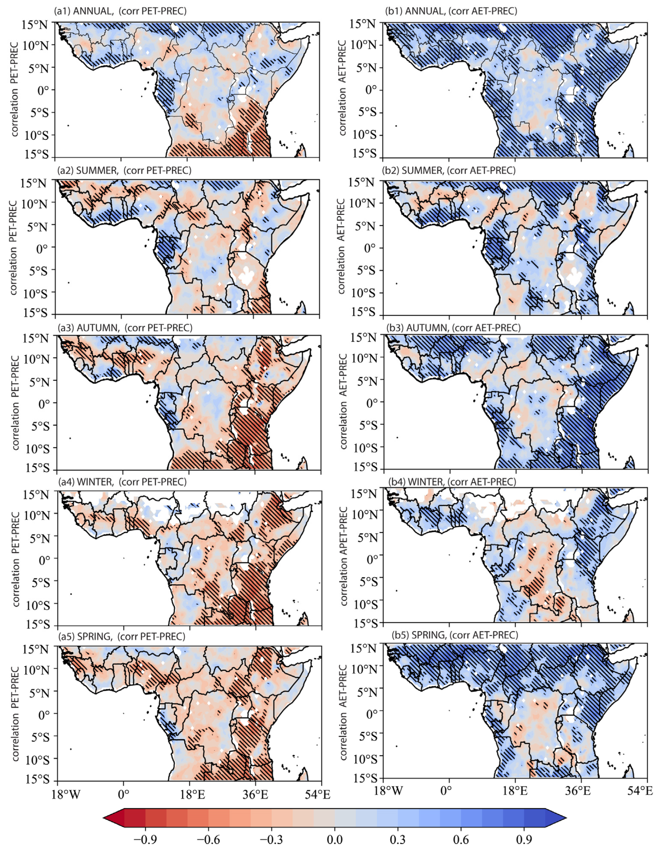
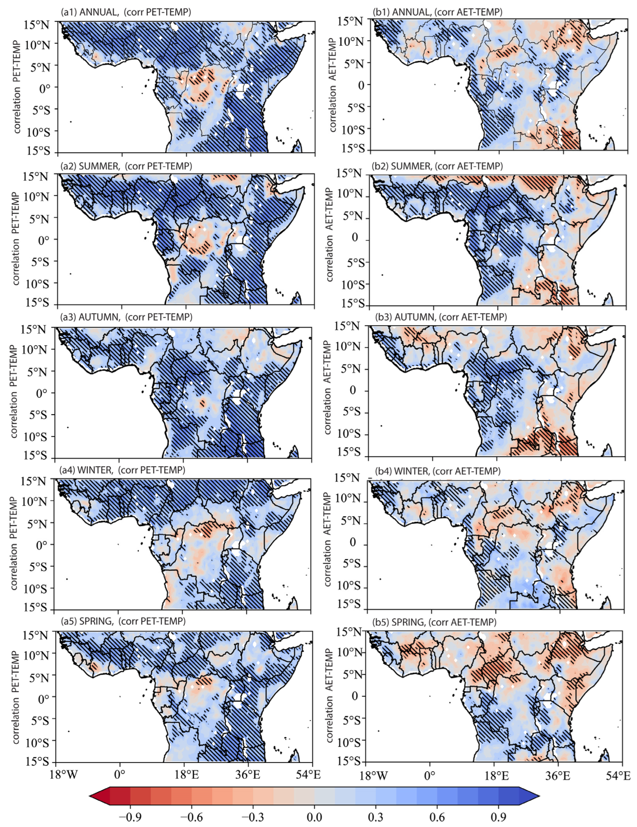
  • The spatial characteristics of the correlations between PET/AET and climatic factors showed an inverse effect in semi-arid/arid conditions, whereas humid conditions showed identical correlation patterns. Humid conditions in the Congo Basin presented a negative spatial extent, with mixed correlation results in semi-arid regions and positive arid conditions. The spatial correlation showed an opposite trend, with increasing PET leading to decreasing AET during 1980–2020. The temporal dynamics revealed that air temperature, soil moisture (SM), and relative humidity are limiting factors that explain the PET/AET temporal dynamics more than precipitation and wind speed.
  • The strong spatial distribution of the correlation is closely linked with global SST anomalies in the tropical Atlantic and Indian Oceans. The spatial correlation pattern is homogenous, with an identical magnitude of correlation values but opposite signs at annual and seasonal scales for both PET and AET variability. By analyzing possible regional atmospheric circulation patterns, the spatial dynamics revealed two major winds (i.e., the northward and southward winds), explaining both PET and AET interannual and seasonal variability.
In summary, our findings from a policy perspective may have implications for future water resource management.

Author Contributions

Conceptualization, I.K.N., F.K.O. and J.L.; methodology, I.K.N. and F.K.O.; software, I.K.N. and F.K.O.; validation, I.K.N., F.K.O. and J.L.; formal analysis, I.K.N. and F.K.O.; investigation, I.K.N. and F.K.O.; data curation, I.K.N., F.K.O., B.A.H. and A.A.S.C.; writing—original draft preparation, I.K.N.; writing—review and editing, B.A.H., L.S., Z.J., A.A.S.C. and F.M.N.; visualization, B.A.H., L.S., Z.J., A.A.S.C. and F.M.N. All authors have read and agreed to the published version of the manuscript.

Funding

This research was funded by the Wuxi University Starting Project 2021r010.

Informed Consent Statement

Not applicable.

Data Availability Statement

The dataset used in this study is publicly available. The GLEAM is accessible via https://www.gleam.eu/ (accessed on 20 March 2022). The ERA5 variables are available at https://cds.climate.copernicus.eu/ (accessed on 20 April 2023). The Climatic Research Unit (CRU) provided the precipitation and air temperature accessible from the CRU website: https://crudata.uea.ac.uk/cru/data/hrg/ (accessed on 10 March 2023). The SST data is at http://ghrsst.jpl.nasa.gov/GHRSST_product_table.html accessed on 20 April 2023.

Acknowledgments

We thank the developers, managers, and funding agencies of the datasets used in this paper for granting access to these datasets, in accordance with their specific data-use and citation policies. acknowledge the administrative and technical support provided by the School of Atmospheric Science and Remote Sensing, Wuxi University, as well as the medical imaging platform with CMOS image sensor (Wuxi University Starting Project 2021r010) and the design of the minimally invasive surgery robot project by the School of Atmospheric Science and Remote Sensing, Wuxi University. Last but not least, thanks to Gnim Tchalim Gnitou, College of Hydrology and Water Resources, Hohai University, Nanjing, Jiangsu, China, for his suggestions and insights into this paper.

Conflicts of Interest

The authors declare no conflict of interest.

Appendix A

Figure A1. Correlation coefficient between PET, AET, and the corresponding soil moisture (root zone) at the annual scale (a1,b1), summer (a2,b2), autumn (a3,b3), winter (a4,b4), and spring (a5,b5) during 1908 to 2020. The hatched area indicates a trend that passes the 0.05 significance test.
Remotesensing 15 03201 g0a1
Figure A2. Correlation coefficient between PET, AET, and the corresponding relative humidity at annual scale (a1,b1), Summer (a2,b2), Autumn (a3,b3), Winter (a4,b4) and Spring (a5,b5) during 1908 to 2020. The hatched area indicates a trend that passes the 0.05 significance test.
Remotesensing 15 03201 g0a2
Figure A3. Correlation coefficient between PET, AET, and the corresponding global SST at the annual scale (a1,b1), summer (a2,b2), autumn (a3,b3), winter (a4,b4), and spring (a5,b5) during 1908 to 2020. The hatched area indicates a trend that passes the 0.05 significance test.
Remotesensing 15 03201 g0a3

References

  1. Fisher, J.B.; Melton, F.; Middleton, E.; Hain, C.; Anderson, M.; Allen, R.; McCabe, M.F.; Hook, S.; Baldocchi, D.; Townsend, P.A.; et al. The future of evapotranspiration: Global requirements for ecosystem functioning, carbon and climate feedbacks, agricultural management, and water resources. Water Resour. Res. 2017, 53, 2618–2626. [Google Scholar] [CrossRef] [Green Version]
  2. Oki, T.; Kanae, S. Global hydrological cycles and world water resources. Science 2006, 313, 1068–1072. [Google Scholar] [CrossRef] [Green Version]
  3. Jasechko, S.; Sharp, Z.D.; Gibson, J.J.; Birks, S.J.; Yi, Y.; Fawcett, P.J. Terrestrial water fluxes dominated by transpiration. Nature 2013, 496, 347–350. [Google Scholar] [CrossRef]
  4. Seneviratne, S.I.; Corti, T.; Davin, E.L.; Hirschi, M.; Jaeger, E.B.; Lehner, I.; Orlowsky, B.; Teuling, A.J. Investigating soil moisture–climate interactions in a changing climate: A review. Earth-Sci. Rev. 2010, 99, 125–161. [Google Scholar] [CrossRef]
  5. Allen, R.G.; Pereira, L.S.; Raes, D.; Smith, M. Crop Evapotranspiration. Guidelines for Computing Crop Water Requirements; FAO Irrigation and Drainage: Rome, Italy, 1998. [Google Scholar]
  6. Teuling, A.J.; Hirschi, M.; Ohmura, A.; Wild, M.; Reichstein, M.; Ciais, P.; Buchmann, N.; Ammann, C.; Montagnani, L.; Richardson, A.D.; et al. A regional perspective on trends in continental evaporation. Geophys. Res. Lett. 2009, 36, L02404. [Google Scholar] [CrossRef] [Green Version]
  7. van Heerwaarden, C.C.; Vilà-Guerau de Arellano, J.; Teuling, A.J. Land-atmosphere coupling explains the link between pan evaporation and actual evapotranspiration trends in a changing climate. Geophys. Res. Lett. 2010, 37, L21401. [Google Scholar] [CrossRef] [Green Version]
  8. Haque, A. Estimating actual areal evapotranspiration from potential evapotranspiration using physical models based on complementary relationships and meteorological data. Bull. Eng. Geol. Environ. 2003, 62, 57–63. [Google Scholar] [CrossRef]
  9. Ghiat, I.; Mackey, H.R.; Al-Ansari, T. A Review of Evapotranspiration Measurement Models, Techniques and Methods for Open and Closed Agricultural Field Applications. Water 2021, 13, 2523. [Google Scholar] [CrossRef]
  10. Wang, S.; Pan, M.; Mu, Q.; Shi, X.; Mao, J.; Bruemmer, C.; Jassal, R.; Krishnan, P.; Li, J.; Black, T. Comparing Evapotranspiration from Eddy Covariance Measurements, Water Budgets, Remote Sensing, and Land Surface Models over Canada. J. Hydrometeorol. 2015, 16, 1540–1560. [Google Scholar] [CrossRef] [Green Version]
  11. Wang, K.; Dickinson, R.E. A review of global terrestrial evapotranspiration: Observation, modeling, climatology, and climatic variability. Rev. Geophys. 2012, 50, RG2005. [Google Scholar] [CrossRef]
  12. Li, Z.-L.; Tang, R.; Wan, Z.; Bi, Y.; Zhou, C.; Tang, B.; Yan, G.; Zhang, X. A Review of Current Methodologies for Regional Evapotranspiration Estimation from Remotely Sensed Data. Sensors 2009, 9, 3801–3853. [Google Scholar] [CrossRef] [Green Version]
  13. Zhang, K.; Kimball, J.S.; Running, S.W. A review of remote sensing based actual evapotranspiration estimation. WIREs Water 2016, 3, 834–853. [Google Scholar] [CrossRef]
  14. Martens, B.; Miralles, D.G.; Lievens, H.; van der Schalie, R.; de Jeu, R.A.M.; Fernández-Prieto, D.; Beck, H.E.; Dorigo, W.A.; Verhoest, N.E.C. GLEAM v3: Satellite-based land evaporation and root-zone soil moisture. Geosci. Model Dev. 2017, 10, 1903–1925. [Google Scholar] [CrossRef] [Green Version]
  15. Miralles, D.G.; Holmes, T.R.H.; De Jeu, R.A.M.; Gash, J.H.; Meesters, A.G.C.A.; Dolman, A.J. Global land-surface evaporation estimated from satellite-based observations. Hydrol. Earth Syst. Sci. 2011, 15, 453–469. [Google Scholar] [CrossRef] [Green Version]
  16. Kiptala, J.K.; Mohamed, Y.; Mul, M.L.; Van der Zaag, P. Mapping evapotranspiration trends using MODIS and SEBAL model in a data scarce and heterogeneous landscape in Eastern Africa. Water Resour. Res. 2013, 49, 8495–8510. [Google Scholar] [CrossRef] [Green Version]
  17. Mu, Q.; Heinsch, F.A.; Zhao, M.; Running, S.W. Development of a global evapotranspiration algorithm based on MODIS and global meteorology data. Remote Sens. Environ. 2007, 111, 519–536. [Google Scholar] [CrossRef]
  18. Mu, Q.; Zhao, M.; Running, S.W. Improvements to a MODIS global terrestrial evapotranspiration algorithm. Remote Sens. Environ. 2011, 115, 1781–1800. [Google Scholar] [CrossRef]
  19. Luo, Y.; Gao, P.; Mu, X. Influence of Meteorological Factors on the Potential Evapotranspiration in Yanhe River Basin, China. Water 2021, 13, 1222. [Google Scholar] [CrossRef]
  20. Jahromi, M.N.; Miralles, D.; Koppa, A.; Rains, D.; Zand-Parsa, S.; Mosaffa, H.; Jamshidi, S. Ten Years of GLEAM: A Review of Scientific Advances and Applications. In Computational Intelligence for Water and Environmental Sciences; Bozorg-Haddad, O., Zolghadr-Asli, B., Eds.; Springer Nature: Singapore, 2022; pp. 525–540. [Google Scholar]
  21. Yang, X.; Wang, G.; Pan, X.; Zhang, Y. Spatio-temporal variability of terrestrial evapotranspiration in china from 1980 to 2011 based on gleam data. Trans. Chin. Soc. Agric. Eng. 2015, 31, 132–141. [Google Scholar]
  22. Nooni, I.K.; Wang, G.; Hagan, D.F.T.; Lu, J.; Ullah, W.; Li, S. Evapotranspiration and its Components in the Nile River Basin Based on Long-Term Satellite Assimilation Product. Water 2019, 11, 1400. [Google Scholar] [CrossRef] [Green Version]
  23. Shijie, L.; Wang, G.; Zhu, C.; Lu, J.; Ullah, W.; Fiifi, D.; Hagan, D.; Kattel, G.; Peng, J. Attribution of global evapotranspiration trends based on the Budyko framework. Hydrol. Earth Syst. Sci. 2022, 26, 3691–3707. [Google Scholar] [CrossRef]
  24. Lu, J.; Wang, G.; Chen, T.; Shijie, L.; Fiifi, D.; Hagan, D.; Kattel, G.; Peng, J.; Tong, J.; Buda, S. A harmonized global land evaporation dataset from model-based products covering 1980–2017. Earth Syst. Sci. Data 2021, 13, 5879–5898. [Google Scholar] [CrossRef]
  25. Lu, J.; Wang, G.; Gong, T.; Hagan, D.; Wang, Y.; Tong, J.; Buda, S. Changes of actual evapotranspiration and its components in the Yangtze River valley during 1980–2014 from satellite assimilation product. Theor. Appl. Climatol. 2019, 138, 1493–1510. [Google Scholar] [CrossRef]
  26. Wang, G.; Pan, J.; Shen, C.; Shijie, L.; Lu, J.; Lou, D.; Hagan, D. Evaluation of Evapotranspiration Estimates in the Yellow River Basin against the Water Balance Method. Water 2018, 10, 1884. [Google Scholar] [CrossRef] [Green Version]
  27. Shijie, L.; Wang, G.; Sun, S.; Hagan, D.; Chen, T.; Dolman, H.; Liu, Y. Long-term changes in evapotranspiration over China and attribution to climatic drivers during 1980–2010. J. Hydrol. 2021, 595, 126037. [Google Scholar] [CrossRef]
  28. Shijie, L.; Wang, G.; Sun, S.; Chen, H.; Peng, B.; Zhou, S.; Huang, Y.; Wang, J.; Deng, P. Assessment of Multi-Source Evapotranspiration Products over China Using Eddy Covariance Observations. Remote Sens. 2018, 10, 1692. [Google Scholar] [CrossRef] [Green Version]
  29. Pour, S.H.; Wahab, A.K.A.; Shahid, S.; Ismail, Z.B. Changes in reference evapotranspiration and its driving factors in peninsular Malaysia. Atmos. Res. 2020, 246, 105096. [Google Scholar] [CrossRef]
  30. Prăvălie, R.; Piticar, A.; Roșca, B.; Sfîcă, L.; Bandoc, G.; Tiscovschi, A.; Patriche, C. Spatio-temporal changes of the climatic water balance in Romania as a response to precipitation and reference evapotranspiration trends during 1961–2013. CATENA 2019, 172, 295–312. [Google Scholar] [CrossRef]
  31. Ahmadi, A.; Daccache, A.; Snyder, R.L.; Suvočarev, K. Meteorological driving forces of reference evapotranspiration and their trends in California. Sci. Total Environ. 2022, 849, 157823. [Google Scholar] [CrossRef] [PubMed]
  32. Xiang, K.; Li, Y.; Horton, R.; Feng, H. Similarity and difference of potential evapotranspiration and reference crop evapotranspiration—A review. Agric. Water Manag. 2020, 232, 106043. [Google Scholar] [CrossRef]
  33. Bouchet, R.J. évapotranspiration réelle et potentielle signification climatique. Int. Assoc. Hydrol. Sci. 1963, 62, 134–142. [Google Scholar]
  34. Chen, Y.; Zhang, S.; Wang, Y. Analysis of the Spatial and Temporal Distribution of Potential Evapotranspiration in Akmola Oblast, Kazakhstan, and the Driving Factors. Remote Sens. 2022, 14, 5311. [Google Scholar] [CrossRef]
  35. Al-Hasani, A.A.J.; Shahid, S. Spatial distribution of the trends in potential evapotranspiration and its influencing climatic factors in Iraq. Theor. Appl. Climatol. 2022, 150, 677–696. [Google Scholar] [CrossRef]
  36. Fu, Z.; Ciais, P.; Prentice, I.C.; Gentine, P.; Makowski, D.; Bastos, A.; Luo, X.; Green, J.K.; Stoy, P.C.; Yang, H.; et al. Atmospheric dryness reduces photosynthesis along a large range of soil water deficits. Nat. Commun. 2022, 13, 989. [Google Scholar] [CrossRef] [PubMed]
  37. Ganeshi, N.G.; Mujumdar, M.; Takaya, Y.; Goswami, M.M.; Singh, B.B.; Krishnan, R.; Terao, T. Soil moisture revamps the temperature extremes in a warming climate over India. NPJ Clim. Atmos. Sci. 2023, 6, 12. [Google Scholar] [CrossRef]
  38. Jung, M.; Reichstein, M.; Margolis, H.A.; Cescatti, A.; Richardson, A.D.; Arain, M.A.; Arneth, A.; Bernhofer, C.; Bonal, D.; Chen, J.; et al. Global patterns of land-atmosphere fluxes of carbon dioxide, latent heat, and sensible heat derived from eddy covariance, satellite, and meteorological observations. J. Geophys. Res. Biogeosc. 2011, 116, G00J07. [Google Scholar] [CrossRef] [Green Version]
  39. Yu, L. A global relationship between the ocean water cycle and near-surface salinity. J. Geophys. Res. Ocean. 2011, 116, C10025. [Google Scholar] [CrossRef]
  40. Hallam, S.; McCarthy, G.D.; Feng, X.; Josey, S.A.; Harris, E.; Düsterhus, A.; Ogungbenro, S.; Hirschi, J.J.M. The relationship between sea surface temperature anomalies, wind and translation speed and North Atlantic tropical cyclone rainfall over ocean and land. Environ. Res. Commun. 2023, 5, 025007. [Google Scholar] [CrossRef]
  41. Gnitou, G.T.; Ma, T.; Tan, G.; Ayugi, B.; Nooni, I.K.; Alabdulkarim, A.; Tian, Y. Evaluation of the Rossby Centre Regional Climate Model Rainfall Simulations over West Africa Using Large-Scale Spatial and Temporal Statistical Metrics. Atmosphere 2019, 10, 802. [Google Scholar] [CrossRef] [Green Version]
  42. Ajibola, F.O.; Zhou, B.; Tchalim Gnitou, G.; Onyejuruwa, A. Evaluation of the Performance of CMIP6 HighResMIP on West African Precipitation. Atmosphere 2020, 11, 1053. [Google Scholar] [CrossRef]
  43. Gnitou, G.T.; Tan, G.; Ma, T.; Akinola, E.O.; Nooni, I.K.; Babaousmail, H.; Al-Nabhan, N. Added value in dynamically downscaling seasonal mean temperature simulations over West Africa. Atmos. Res. 2021, 260, 105694. [Google Scholar] [CrossRef]
  44. Ayugi, B.; Dike, V.; Nadoya, H.N.; Babaousmail, H.; Mumo, R.; Ongoma, V. Future Changes in Precipitation Extremes over East Africa Based on CMIP6 Models. Water 2021, 13, 2358. [Google Scholar] [CrossRef]
  45. Ayugi, B.; Ngoma, H.; Babaousmail, H.; Karim, R.; Iyakaremye, V.; Lim Kam Sian, K.T.C.; Ongoma, V. Evaluation and projection of mean surface temperature using CMIP6 models over East Africa. J. Afr. Earth Sci. 2021, 181, 104226. [Google Scholar] [CrossRef]
  46. Ayugi, B.; Tan, G.; Gnitou, G.T.; Ojara, M.; Ongoma, V. Historical evaluations and simulations of precipitation over East Africa from Rossby centre regional climate model. Atmos. Res. 2020, 232, 104705. [Google Scholar] [CrossRef]
  47. Tamoffo, A.T.; Vondou, A.; Pokam, W.; Haensler, A.; Djomou, Z.; Fotso-Nguemo, T.C.; Tchotchou, L.; Nouayou, R. Daily characteristics of Central African rainfall in the REMO model. Theor. Appl. Climatol. 2019, 137, 2351–2368. [Google Scholar] [CrossRef]
  48. Dommo, A.; Vondou, A.; Philippon, N.; Eastman, R.; Moron, V.; Aloysius, N. The ERA5′s diurnal cycle of low-level clouds over Western Central Africa during June–September: Dynamic and thermodynamic processes. Atmos. Res. 2022, 280, 106426. [Google Scholar] [CrossRef]
  49. Taguela, T.; Pokam, W.; Washington, R. Rainfall in uncoupled and coupled versions of the Met Office Unified Model over Central Africa: Investigation of processes during the September–November rainy season. Int. J. Climatol. 2022, 42, 6311–6331. [Google Scholar] [CrossRef]
  50. Iturbide, M.; Gutiérrez, J.M.; Alves, L.M.; Bedia, J.; Cerezo-Mota, R.; Cimadevilla, E.; Cofiño, A.S.; Di Luca, A.; Faria, S.H.; Gorodetskaya, I.V.; et al. An update of IPCC climate reference regions for subcontinental analysis of climate model data: Definition and aggregated datasets. Earth Syst. Sci. Data 2020, 12, 2959–2970. [Google Scholar] [CrossRef]
  51. Ateba Boyomo, H.; Emmanuel, O.; William, M.; Asngar, T. Does climate change influence conflicts? Evidence for the Cameroonian regions. GeoJournal 2023. [Google Scholar] [CrossRef]
  52. Ongoma, V.; Chen, H.; Gao, C. Projected changes in mean rainfall and temperature over East Africa based on CMIP5 models. Int. J. Climatol. 2018, 38, 1375–1392. [Google Scholar] [CrossRef]
  53. Flaounas, E.; Bastin, S.; Janicot, S. Regional climate modelling of the 2006 West African monsoon: Sensitivity to convection and planetary boundary layer parameterisation using WRF. Clim. Dyn. 2011, 36, 1083–1105. [Google Scholar] [CrossRef]
  54. Raj, J.; Bangalath, H.K.; Stenchikov, G. West African Monsoon: Current state and future projections in a high-resolution AGCM. Clim. Dyn. 2019, 52, 6441–6461. [Google Scholar] [CrossRef] [Green Version]
  55. Kothe, S.; Lüthi, D.; Ahrens, B. Analysis of the West African Monsoon system in the regional climate model COSMO-CLM. Int. J. Climatol. 2014, 34, 481–493. [Google Scholar] [CrossRef]
  56. Lafore, J.-P.; Flamant, C.; Guichard, F.; Parker, D.J.; Bouniol, D.; Fink, A.H.; Giraud, V.; Gosset, M.; Hall, N.; Höller, H.; et al. Progress in understanding of weather systems in West Africa. Atmos. Sci. Lett. 2011, 12, 7–12. [Google Scholar] [CrossRef] [Green Version]
  57. Brandt, P.; Caniaux, G.; Bourlès, B.; Lazar, A.; Dengler, M.; Funk, A.; Hormann, V.; Giordani, H.; Marin, F. Equatorial upper-ocean dynamics and their interaction with the West African monsoon. Atmos. Sci. Lett. 2011, 12, 24–30. [Google Scholar] [CrossRef] [Green Version]
  58. Miralles, D.G.; De Jeu, R.A.M.; Gash, J.H.; Holmes, T.R.H.; Dolman, A.J. Magnitude and variability of land evaporation and its components at the global scale. Hydrol. Earth Syst. Sci. 2011, 15, 967–981. [Google Scholar] [CrossRef] [Green Version]
  59. Miralles, D.G.; van den Berg, M.J.; Gash, J.H.; Parinussa, R.M.; de Jeu, R.A.M.; Beck, H.E.; Holmes, T.R.H.; Jiménez, C.; Verhoest, N.E.C.; Dorigo, W.A.; et al. El Niño–La Niña cycle and recent trends in continental evaporation. Nat. Clim. Change 2014, 4, 122–126. [Google Scholar] [CrossRef]
  60. Priestley, C.H.B.; Taylor, R.J. On the assessment of surface heat flux and evapotranspiration using large scale parameters. Mon. Weather Rev. 1972, 100, 81–92. [Google Scholar] [CrossRef]
  61. European Center for Medium-Range Weather Forecasts (ECMWF). Home Page. Available online: http://apps.ecmwf.int/datasets/data/interim-full-daily/levtype=sfc/ (accessed on 20 April 2023).
  62. Hersbach, H.; Bell, B.; Berrisford, P.; Hirahara, S.; Horányi, A.; Muñoz-Sabater, J.; Nicolas, J.; Peubey, C.; Radu, R.; Schepers, D.; et al. The ERA5 global reanalysis. Q. J. R. Meteorol. Soc. 2020, 146, 1999–2049. [Google Scholar] [CrossRef]
  63. Bell, B.; Hersbach, H.; Simmons, A.; Berrisford, P.; Dahlgren, P.; Horányi, A.; Muñoz-Sabater, J.; Nicolas, J.; Radu, R.; Schepers, D.; et al. The ERA5 global reanalysis: Preliminary extension to 1950. Q. J. R. Meteorol. Soc. 2021, 147, 4186–4227. [Google Scholar] [CrossRef]
  64. Lavers, D.A.; Simmons, A.; Vamborg, F.; Rodwell, M.J. An evaluation of ERA5 precipitation for climate monitoring. Q. J. R. Meteorol. Soc. 2022, 148, 3152–3165. [Google Scholar] [CrossRef]
  65. Silvestri, L.; Saraceni, M.; Bongioannini Cerlini, P. Links between precipitation, circulation weather types and orography in central Italy. Int. J. Climatol. 2022, 42, 5807–5825. [Google Scholar] [CrossRef]
  66. Chen, A.; Chen, D.; Azorin-Molina, C. Assessing reliability of precipitation data over the Mekong River Basin: A comparison of ground-based, satellite, and reanalysis datasets. Int. J. Climatol. 2018, 38, 4314–4334. [Google Scholar] [CrossRef]
  67. Hu, X.; Yuan, W. Evaluation of ERA5 precipitation over the eastern periphery of the Tibetan plateau from the perspective of regional rainfall events. Int. J. Climatol. 2021, 41, 2625–2637. [Google Scholar] [CrossRef]
  68. Assamnew, A.D.; Mengistu Tsidu, G. Assessing improvement in the fifth-generation ECMWF atmospheric reanalysis precipitation over East Africa. Int. J. Climatol. 2023, 43, 17–37. [Google Scholar] [CrossRef]
  69. CRU. The Climatic Research Unit (CRU) Precipitation and air Temperature Hompage. Available online: https://crudata.uea.ac.uk/cru/data/hrg/ (accessed on 10 March 2023).
  70. Harris, I.; Osborn, T.J.; Jones, P.; Lister, D. Version 4 of the CRU TS monthly high-resolution gridded multivariate climate dataset. Sci. Data 2020, 7, 109. [Google Scholar] [CrossRef] [Green Version]
  71. Onyutha, C. Trends and variability in African long-term precipitation. Stoch. Environ. Res. Risk Assess. 2018, 32, 2721–2739. [Google Scholar] [CrossRef]
  72. GHRSST. Global Data Assembly Center (GDAC) at the Jet Propulsion Laboratory (JPL) Physical Oceanography Distributed Active Archive Center (PO.DAAC) Homepage. Available online: http://ghrsst.jpl.nasa.gov/GHRSST_product_table.html (accessed on 20 April 2023).
  73. Harris, I.; Jones, P.D.; Osborn, T.J.; Lister, D.H. Updated high-resolution grids of monthly climatic observations—The CRU TS3.10 Dataset. Int. J. Climatol. 2014, 34, 623–642. [Google Scholar] [CrossRef] [Green Version]
  74. Harris, I.C.; Jones, P.D.; Osbon, T. CRU TS4.04: Climate Research Unit (CRU) Time-Series (TS) Version 4.04 of Highresolution Gridded Data of Monthly-by-Monthly Variation in Climate (January 1901–December 2019). Available online: https://catalogue.ceda.ac.uk/uuid/89e1e34ec3554dc (accessed on 10 March 2023).
  75. Mann, H.B. Nonparametric Tests Against Trend. Econometrica 1945, 13, 245–259. [Google Scholar] [CrossRef]
  76. Kendall, M.G. Rank correlation methods. Griffin, London. J. Econom. 1975, 13, 245–259. [Google Scholar]
  77. Theil, H. A rank invariant method of linear and polynomial regression analysis. Proc. Ned. Akad. Wet. 1950, 53, 1397–1412. [Google Scholar]
  78. Sen, P.K. Estimates of the Regression Coefficient Based on Kendall’s Tau. J. Am. Stat. Assoc. 1968, 63, 1379–1389. [Google Scholar] [CrossRef]
  79. van de Schoot, R.; Depaoli, S.; King, R.; Kramer, B.; Märtens, K.; Tadesse, M.G.; Vannucci, M.; Gelman, A.; Veen, D.; Willemsen, J.; et al. Bayesian statistics and modelling. Nat. Rev. Methods Prim. 2021, 1, 1. [Google Scholar] [CrossRef]
  80. Fan, Y.; Lu, X. An online Bayesian approach to change-point detection for categorical data. Knowl.-Based Syst. 2020, 196, 105792. [Google Scholar] [CrossRef]
  81. Kortsch, S.; Primicerio, R.; Beuchel, F.; Renaud, P.E.; Rodrigues, J.; Lønne, O.J.; Gulliksen, B. Climate-driven regime shifts in Arctic marine benthos. Proc. Natl. Acad. Sci. USA 2012, 109, 14052–14057. [Google Scholar] [CrossRef] [Green Version]
  82. Samhouri, J.F.; Andrews, K.S.; Fay, G.; Harvey, C.J.; Hazen, E.L.; Hennessey, S.M.; Holsman, K.; Hunsicker, M.E.; Large, S.I.; Marshall, K.N.; et al. Defining ecosystem thresholds for human activities and environmental pressures in the California Current. Ecosphere 2017, 8, e01860. [Google Scholar] [CrossRef] [Green Version]
  83. Yao, T.; Lu, H.; Feng, W.; Yu, Q. Evaporation abrupt changes in the Qinghai-Tibet Plateau during the last half-century. Sci. Rep. 2019, 9, 20181. [Google Scholar] [CrossRef] [Green Version]
  84. Wang, J.; Wang, Q.; Zhao, Y.; Li, H.; Zhai, J.; Shang, Y. Temporal and spatial characteristics of pan evaporation trends and their attribution to meteorological drivers in the Three-River Source Region, China. J. Geophys. Res. Atmos. 2015, 120, 6391–6408. [Google Scholar] [CrossRef]
  85. Zhang, Y.; Liu, C.; Tang, Y.; Yang, Y. Trends in pan evaporation and reference and actual evapotranspiration across the Tibetan Plateau. J. Geophys. Res. Atmos. 2007, 112, D12110. [Google Scholar] [CrossRef]
  86. Li, Z.; Wang, S.; Li, J. Spatial variations and long-term trends of potential evaporation in Canada. Sci. Rep. 2020, 10, 22089. [Google Scholar] [CrossRef]
  87. Wang, S.; Yang, Y.; Luo, Y.; Rivera, A. Spatial and seasonal variations in evapotranspiration over Canada’s landmass. Hydrol. Earth Syst. Sci. 2013, 17, 3561–3575. [Google Scholar] [CrossRef] [Green Version]
  88. Nouri, M.; Bannayan, M. Spatiotemporal changes in aridity index and reference evapotranspiration over semi-arid and humid regions of Iran: Trend, cause, and sensitivity analyses. Theor. Appl. Climatol. 2019, 136, 1073–1084. [Google Scholar] [CrossRef]
  89. Cabral Júnior, J.B.; Silva, C.M.S.e.; de Almeida, H.A.; Bezerra, B.G.; Spyrides, M.H.C. Detecting linear trend of reference evapotranspiration in irrigated farming areas in Brazil’s semiarid region. Theor. Appl. Climatol. 2019, 138, 215–225. [Google Scholar] [CrossRef]
  90. Rahman, M.A.; Yunsheng, L.; Sultana, N.; Ongoma, V. Analysis of reference evapotranspiration (ET0) trends under climate change in Bangladesh using observed and CMIP5 data sets. Meteorol. Atmos. Phys. 2019, 131, 639–655. [Google Scholar] [CrossRef]
  91. Mueller, B.; Seneviratne, S.I.; Jimenez, C.; Corti, T.; Hirschi, M.; Balsamo, G.; Ciais, P.; Dirmeyer, P.; Fisher, J.B.; Guo, Z.; et al. Evaluation of global observations-based evapotranspiration datasets and IPCC AR4 simulations. Geophys. Res. Lett. 2011, 38, L06402. [Google Scholar] [CrossRef] [Green Version]
  92. Hobbins, M.T.; Ramirez, J.A.; Brown, T.C. Trends in pan evaporation and actual evapotranspiration across the conterminous US: Paradoxical or complementary? Geophys. Res. Lett. 2004, 316, L13503. [Google Scholar] [CrossRef] [Green Version]
  93. Ramirez, J.A.; Hobbins, M.T.; Brown, T.C. Observational evidence of the complementary relationship in regional evaporation lends strong support for Bouchet’s hypothesis. Geophys. Res. Lett. 2005, 32, L15401. [Google Scholar] [CrossRef] [Green Version]
  94. Golubev, V.S.; Lawrimore, J.H.; Groisman, P.Y.; Speranskaya, N.A.; Zhuravin, S.A.; Menne, M.J.; Peterson, T.C.; Malone, R.W. Evaporation changes over the contiguous United States and the former USSR: A reassessment. Geophys. Res. Lett. 2001, 28, 2665–2668. [Google Scholar] [CrossRef]
  95. Roderick, M.L.; Rotstayn, L.D.; Farquhar, G.D.; Hobbins, M.T. On the attribution of changing pan evaporation. Geophys. Res. Lett. 2007, 34, L17403. [Google Scholar] [CrossRef] [Green Version]
  96. Stephens, C.M.; McVicar, T.R.; Johnson, F.M.; Marshall, L.A. Revisiting Pan Evaporation Trends in Australia a Decade on. Geophys. Res. Lett. 2018, 45, 11164–11172. [Google Scholar] [CrossRef]
  97. Verstraeten, W.W.; Veroustraete, F.; Feyen, J. Assessment of Evapotranspiration and Soil Moisture Content Across Different Scales of Observation. Sensors 2008, 8, 70–117. [Google Scholar] [CrossRef] [PubMed] [Green Version]
  98. Yang, Y.; Roderick, M.L. Radiation, surface temperature and evaporation over wet surfaces. Q. J. R. Meteorol. Soc. 2019, 145, 1118–1129. [Google Scholar] [CrossRef]
  99. Adnan, S.; Ullah, K.; Ahmed, R. Variability in meteorological parameters and their impact on evapotranspiration in a humid zone of Pakistan. Meteorol. Appl. 2020, 27, e1859. [Google Scholar] [CrossRef] [Green Version]
  100. Alley, R.B. Abrupt climate change. Science 2003, 299, 2005–2010. [Google Scholar] [CrossRef] [PubMed] [Green Version]
  101. Severinghaus, J.P.; Sowers, T.; Brook, E.J.; Alley, R.B.; Bender, M.L. Timing of abrupt climate change at the end of the Younger Dryas interval from thermally fractionated gases in polar ice. Nature 1998, 391, 141–146. [Google Scholar] [CrossRef]
  102. McIntyre, M.E. Climate tipping points: A personal view. Phys. Today 2023, 76, 44–49. [Google Scholar] [CrossRef]
Figure 1. The study area map of Equatorial Africa. (a) Elevation (m); (b) annual precipitation (mm) and (c) temperature (°C).
Remotesensing 15 03201 g001
Figure 2. Spatial pattern means PET (a1a4) and AET (b1b4) for annual (a1,b1), summer (a2,b2), autumn (a3,b3), winter (a4,b4), and spring (a5,b5) from 1980 to 2020. The unit is mm.
Remotesensing 15 03201 g002
Figure 3. The annual cycles of PET (red color) and AET (blue color) averaged from 1980 to 2020.
Remotesensing 15 03201 g003
Figure 4. Linear trends in annual PET (a1) and AET (b1) and seasonal PET (a2a5) and AET (b2b5) during 1980–2020 across EQA. A positive sign denotes an upward trend, and a negative value indicates a significant downward trend at p < 0.05.
Remotesensing 15 03201 g004
Figure 5. Spatial patterns of annual and seasonal linear trends in PET and AET during 1980–2020 across EQA. Annual trends in PET (a1) and annual AET (b1). Seasonal PET (a2a5) and AET (b2b5). The hatched lines denote a linear trend significant at p < 0.05.
Remotesensing 15 03201 g005
Figure 6. Abrupt climate changes in annual mean PET (top panel) and AET (bottom panel) during 1980–2020 across EQ. Africa using the Bayesian test. The blue dashed line indicates the year the change occurred with a probability of less than 0.05.
Remotesensing 15 03201 g006
Figure 7. The correlation coefficient between PET, AET, and the corresponding precipitation at the annual scale (a1,b1), summer (a2,b2), autumn (a3,b3), winter (a4,b4), and spring (a5,b5) during 1908 to 2020. The hatched area indicates a trend passing the 0.05 significance test.
Remotesensing 15 03201 g007
Figure 8. The correlation coefficient between PET, AET and the corresponding mean air temperature at the annual scale (a1,b1), summer (a2,b2), autumn (a3,b3), winter (a4,b4), and spring (a5,b5) during 1980 to 2020. The hatched area indicates a trend passing the 0.05 significance test.
Remotesensing 15 03201 g008
Figure 9. The correlation coefficient between PET, AET, and the corresponding wind speed (10 ms−1) at the annual scale (a1,b1), summer (a2,b2), autumn (a3,b3), winter (a4,b4), and spring (a5,b5) during 1980 to 2020. The hatched area indicates a trend passing the 0.05 significance test.
Remotesensing 15 03201 g009
Figure 10. Heatmap plots comparing temporal correlation coefficients (r) of mean evaporation (actual and potential) during 1980–2020. The correlation coefficient is significant at the 5% level.
Remotesensing 15 03201 g010
Figure 11. Spatial distributions of correlation coefficients of PET and AET and SST at the annual scale (a1,b1), summer (a2,b2), autumn (a3,b3), winter (a4,b4), and spring (a5,b5) during 1908 to 2020. The hatched area indicates a trend passing the 0.05 significance test.
Remotesensing 15 03201 g011
Figure 12. Climatology of wind circulation at 850 pha over equatorial Africa from 1980 to 2020. annual scale (a), summer (b), autumn (c), winter (d), and spring (e).
Remotesensing 15 03201 g012
Table 1. Seasonal climatology of meteorological variables in EQ. Africa (i.e., averaged over longitude: 18°W–55°E and latitude: 15°S–15°N).
ParametersAnnualSummerAutumnWinterSpring
Air temperature (°C)25.28024.95024.91424.91425.318
Precipitation (mm)89.66276.84090.78497.84790.843
Relative humidity (%)70.34266.10869.59873.08172.328
Soil moisture (m3m−3)0.2590.2520.2560.2640.261
Wind speed (ms−1)3.8123.4443.3264.5603.595
Table 2. Temporal correlation coefficients (r) between evapotranspiration (actual and potential) and six environmental and climate factors for 1980–2020. Absolute r greater than 0.30 is significant at the 5% level.
ParameterAETPET
Air temperature (°C)−0.580.79
Precipitation (mm)0.060.25
Relative humidity (%)0.70−0.81
Soil moisture (m3 m−3)0.86−0.65
Wind speed (ms−1)−0.400.33
Disclaimer/Publisher’s Note: The statements, opinions and data contained in all publications are solely those of the individual author(s) and contributor(s) and not of MDPI and/or the editor(s). MDPI and/or the editor(s) disclaim responsibility for any injury to people or property resulting from any ideas, methods, instructions or products referred to in the content.

