
Accuracy Assessment of Eleven Medium Resolution Global and Regional Land Cover Land Use Products: A Case Study over the Conterminous United States


Department of Environmental Resources Engineering, State University of New York College of Environmental Science and Forestry, Syracuse, NY 13210, USA
*
Author to whom correspondence should be addressed.
Remote Sens. 2023, 15(12), 3186; https://doi.org/10.3390/rs15123186
Submission received: 1 May 2023
/
Revised: 5 June 2023
/
Accepted: 15 June 2023
/
Published: 19 June 2023
(This article belongs to the Section Earth Observation Data)
Abstract
:Land cover land use (LCLU) products provide essential information for numerous environmental and human studies. Here, we assess the accuracy of eleven global and regional products over the conterminous U.S. using 25,000 high-confidence randomly distributed samples. Results show that in general, the National Land Cover Database (NLCD) and the Land Change Monitoring, Assessment and Projection (LCMAP) outperform other multi-class products, both in terms of higher individual class accuracy and with accuracy variability across classes. More specifically, F1 accuracy comparisons between the best performing USGS and non-USGS products indicate: (i) similar performance for the water class, (ii) USGS product outperformance in the developed (+1.3%), grass/shrub (+3.2%) and tree cover (+4.2%) classes, and (iii) non-USGS product (WorldCover) gains in the cropland (+5.1%) class. The NLCD and LCMAP also outperformed specialized single-class products, such as the Hansen Global Forest Change, the Cropland Data Layer and the Global Artificial Impervious Areas, while offering comparable results to the Global Surface Water Dynamics product. Spatial visualizations also allowed accuracy comparisons across different geographic areas. In general, the NLCD and LCMAP have disagreements mainly in the middle and southeastern part of conterminous U.S. while Esri, WorldCover and Dynamic World have most errors in the western U.S. Comparisons were also undertaken on a subset of the reference data, called spatial edge samples, that identifies samples surrounded by neighboring samples of different class labels, thus excluding easy-to-classify homogenous areas. There, the WorldCover product offers higher accuracies for the highly dynamic grass/shrub (+4.4%) and cropland (+8.1%) classes when compared to the NLCD and LCMAP products. An important conclusion while looking at these challenging samples is that except for the tree class (78%), the best performing products per class range in accuracy between 55% and 70%, which suggests that there is substantial room for improvement.
1. Introduction
Land cover and land use (LCLU) products offer significant biophysical information on the Earth’s surface [1]. They are essential for various studies, such as biogeochemical and climate cycles [2], earth system models [3], desertification and biological diversity [4] and environmental resources management [5]. The considerable impact of LCLU products has led to mapping efforts ranging from local to global extents.
The global extent LCLU maps have ranged in spatial resolution from 10 m to 1 km. Global mapping products include the following examples, progressively presented from coarser to finer spatial resolution as shown in Table 1: the International Geosphere-Biosphere Program Data and Information System’s land cover product (IGBP DISCover), 1992–1993, 1 km resolution [6,7]; the University of Maryland land cover product (UMD), 1992–1993, 1 km resolution [8]; the Global Land Cover 2000 product (GLC) from the European Commission’s Joint Research Center (JRC) at 1 km resolution [9]; the Moderate Resolution Imaging Spectroradiometer (MODIS) land cover product (MOD12Q1 and MCD12Q1) available at annual scale from 2001, with 500/1000 m resolution [10,11]; the Global Map–Global land cover (GLCNMO) product from the International Steering Committee for Global Mapping, 2003/2008 at 500 m resolution [12]; the Global land cover Map (GlobCover) from the European Space Agency (ESA), 2005–2006/2009 at 300 m resolution [13,14]; the Finer Resolution Observation and Monitoring Global LC product (FROM-GLC) from China, 2010/2015/2017 at 30 m resolution [15,16]; the 30 m resolution Global land cover product (GlobeLand30) from the National Geomatics Center of China, 2000/2010 [17]; the Global map of land use/land cover (LULC) from Esri, 2017–2021 at 10 m resolution [18]; the World Cover from European Space Agency (ESA), 2020/2021 at 10 m resolution [19,20]; and the Dynamic World from Google, 2015–2023, at 10 m resolution [21].
Within our study area of the conterminous United States, several regional products exist, primarily led by the U.S. Geological Survey (USGS). One representative product is the 30 m resolution National Land Cover Database (NLCD) covering multiple years (1992/2001/2006/2011/2016/2019) [22]. There are also some annual products based on Landsat data: the 30 m resolution Landscape Change Monitoring System (LCMS) from the USDA Forest Service (USFS), annual since 1985 [23]; and the 30 m resolution Land Change Monitoring, Assessment and Projection (LCMAP) from USGS, offering annual changes since 1985 [24].
As collecting validation samples is labor-intensive work, the size of validation data is usually small. However, a few large validation datasets exist. For example, Land Use/Cover Area frame statistical Survey (LUCAS) validation data are a systematic sample with 1.1 million points spaced 2 km apart in the four cardinal directions covering the entire European Union (EU) [25]. The World Cover validation dataset includes more than 21,000 primary sampling units (PSUs) spread over seven (sub)continents and each PSU contains 100 secondary sample units (SSUs) corresponding to pixels with 10 m resolution [20]. The LCMAP reference dataset by USGS is another pixel-based validation dataset containing 25,000 samples with land use and land cover information annually from 1984 to 2018. Due to its multi-year presence, labeling consistency and large sample size over the conterminous U.S., our study incorporated the LCMAP reference validation dataset.
The LCLU products may vary widely as different satellite data, classification schemes and classification approaches are implemented [26] and intended usage may deviate. Therefore, accuracy assessment of different LCLU products is essential to assist users understand benefits/limitations and guide suitable product selection. In general, the accuracy assessment of large scale LCLU maps follows the trajectory of large-scale maps becoming more detailed from coarser to finer resolution. For example, four 1 km resolution global land cover products ((IGBP DISCover, UMD, MODIS and GLC2000) were compared and assessed [27], five global land cover products (GLCC, UMD, GLC2000, MODIS LC and GlobCover) from 1 km to 500 m resolution around year 2000 were assessed over China [28]. Three global products (Globcover, LC-CCI and MODIS) were compared at 300 m resolution for the year 2005 [29], while seven global products (IGBP DISCover, UMD, GLC, MCD12Q1, GLCNMO, CCI-LC and GlobeLand30) including resolution from 1 km to 30 m were assessed over China [26]. Liang et al. [30] evaluated four global land cover products (GlobeLand30, CCI-LC, GLCNMO and MODIS) over the Arctic region. Gao et al. [31] compared three global products (GlobeLand30-2010, GLC_FCS30-2015 and FROM_GLC30-2015) over the European Union. Zhang et al. [32] compared accuracies of six 30 m cropland products (FROM-GLC, GLC_FCS, CLCD, AGLC, GFSAD and GLAD) over China in year 2015.
In the aforementioned studies, there are several knowledge gaps:
- (i).
- There is no study explicitly evaluating global LCLU products over the conterminous U.S.
- (ii).
- None of the prior studies assessed accuracy differences over time for products available at multiple time periods.
- (iii).
- None of the prior studies looked at accuracy behavior explicitly in land spatial edge pixels, a more challenging classification task due to potential spectral mixing.
Therefore, the goal of this study is to compare and evaluate eleven medium resolution global and regional LCLU mapping products over the conterminous U.S., both spatially and temporally. In the next sections we present the reference dataset and the compared global and regional LCLU followed by implemented methods including classification scheme matching, spatial reprojection and spatial accuracy assessment in Section 3. Results are displayed and discussed in Section 4 and conclusions are summarized in Section 5.
2. Materials
In the next sections we first present the accuracy assessment reference dataset followed by the products that were evaluated on it.
2.1. Reference Dataset for Product Evaluation
The reference validation samples data used in this study come from the LCMAP conterminous United States Reference Data Product, freely available from the USGS [33]. The LCMAP reference dataset contains 25,000 Landsat 30 m resolution pixels randomly selected from pixels in the continental U.S. ARD grid system with annual labels from 1984 to 2018 [34]. The reference data were a cooperation between the USGS LCMAP group and the U.S. Forest Service Landscape Change Monitoring System (LCMS, 2021). Annotation protocols were established in a Joint Response Design (JRD) document [35] under the data requirements of both projects. A team of interpreters assigned the class labels of reference sample pixels by following a common response design using a special reference data collection tool called the TimeSync [36,37], which shows all available Landsat data, including anniversary date images for each year for interpreters. Interpreters visually interpreted each sample pixel and determined land use, land cover and change process attribute labels for every year which were bridged to LCMAP classes. The LCMAP reference data has consistent high quality due to various quality assurance and quality control (QA/QC) processes. The interpreters’ overall agreement was 88% and average individual class agreement ranged from 62% for barren to 94% for water (with lower agreement of 74% for wetland and higher agreement over 81% for other classes) [37]. The barren and wetland had lower interpreter agreements since the they were represented less. Since a lower agreement of reference data may influence accuracy assessment results, users should be careful with results of barren and wetland classes. However, the effects should not be significant as the overall agreement is high. In this study, 24,971 samples were used as there are 29 samples falling outside of LCMAP area. We extracted seven thematic class labels from LCMAP for the assessment, namely: Developed, Cropland, Grass/Shrub, Tree cover, Water, Wetland and Barren. Table 2 shows the number of samples for each class for the overall dataset and a subset containing spatial edge samples. Spatial edge samples are defined as the samples where at least one of its eight neighborhood pixels has a different class label from the center sample. It was calculated using the NLCD 2016 dataset as results later indicated this was the most accurate product. While the NLCD 2016 product was used and we have no way of explicitly identifying its accuracy on those 3 × 3 patches, the accuracy drop reported in spatial edge pixels implicitly suggests that these were indeed heterogenous patches. The intent behind accuracy comparisons on spatial edge pixels is to identify samples in heterogenous land cover areas where classification tasks tend to be more challenging.
Misclassifications due to geolocation errors might be challenging for pixel-based accuracy assessment, when the reference and product pixels are not perfectly lined up [34]. However, the other method of using block units such as with 3 × 3 pixels instead of a single pixel was criticized by [38] since the accuracy for such block units does not represent the accuracy of the map provided to users. In our study, we chose to perform our analysis at pixel level. In the next sections we investigated the selected products. The product selection criteria were based on the LCMAP reference dataset characteristics such as cell size, temporal availability and class definitions.
2.2. Global Multi-Class LCLU Products
The Finer Resolution Observation and Monitoring of Global Land Cover (FROM-GLC) are the first 30 m resolution global land cover maps produced by Department of Earth System Science of Tsinghua University using Landsat Thematic Mapper (TM) and Enhanced TM plus (ETM+) data with a total number of 8929 scenes. The FROM-GLC product was generated by four classifiers, namely a conventional maximum likelihood classifier (MLC), a J4.8 decision tree classifier, a Random Forest (RF) classifier and a support vector machine (SVM) classifier with the highest overall classification accuracy of 64.9% produced by SVM and second high of 59.8% by RF [15]. It developed a unique land cover classification scheme which is able to be cross-walked to the existing United Nations Food and Agriculture Organization (FAO) land cover classification scheme and the International Geosphere-Biosphere Program (IGBP) scheme and it includes two levels of classification with 10 level-1 classes and 29 level-2 classes for years of 2010, 2015 and 2017 [15,39]. In this study, we chose data for the years 2010 and 2015 so that they can be comparable to other products available in the same years. We excluded the year 2017 since it is close to 2015; we evaluated products using a common temporal baseline with a 5-year interval starting from 1990.
GlobeLand30 is a 30 m resolution global land cover data product under the ‘Global Land Cover Mapping at Finer Resolution’ project that was developed by the National Geomatics Center of China (NGCC). The GlobeLand30 product has been produced for two years of 2000 and 2010 [40] and was produced based on more than 10,000 scenes primarily from the Landsat Thematic Mapper (TM) and Enhanced TM plus (ETM+) satellites. Images from the Chinese Environmental and Disaster (HJ-1) satellite were also considered for the year of 2010. Unlike FROM-GLC, a pixel-object-knowledge-based (POK-based) classification approach was implemented to create this product achieving an overall accuracy of over 80% [17,41]. GlobeLand30 adopted a classification scheme with 10 land cover types: water bodies, wetlands, artificial surfaces, cultivated lands, forests, shrublands, grasslands, and barren lands [17,42]. In this study, we choose both years of 2000 and 2010 data to compare spatially and temporally with other products.
ESRI ‘s Sentinel-2 10 m land cover time series product provides annual global LCLU maps from 2017 to 2021. The Impact Observatory’s deep learning AI land classification model was used to create the products. It is trained on a very large reference dataset comprised of over 24,000 5 km × 5 km Sentinel-2 image patches with resolution of 10 m. It contains ten classes, namely water, trees, grass, flooded vegetation, crops, scrub/shrub, built area, bare ground, snow/ice, and clouds [18]. Data were collected across 14 major biomes employing a random stratified sampling approach. An overall accuracy of 85% was achieved over a set of tiles labeled by multiple expert annotators over 409 5 km × 5 km sample areas.
World Cover is a global land cover product developed by the European Space Agency at 10 m resolution based on both Sentinel-1 and Sentinel-2 data with eleven classes (Built-up, Cropland, Grassland, Shrubland, Moss and lichen, Tree cover, Permanent water bodies, Herbaceous wetland, Mangroves, Snow and Ice, and Bare). The ESA World Cover product provides two years of global land cover data: 2020 and 2021 and it uses a random forest classification tree algorithm with a global overall accuracy of 74.4% for 2020 and 76.7% for 2021 using an independently validation product [20].
Dynamic World is the first near real-time global LCLU product. It is developed by Google at 10 m resolution based on Sentinel-2 data, and it delivers near real-time LCLU products in parallel with Sentinel-2 acquisitions (every 5 days). It is based on deep learning models with a training data over 5 billion hand labeled pixel patches from 24,000 individual image tiles (510 × 510 pixels each) with resolution of 10 m distributed over the world which is the same reference dataset of Esri’s product. Other than single pixel labels, annotators use dense markup of vector boundaries around individual classes. It includes nine classes: water, trees, grass, flooded vegetation, crops, scrub/shrub, built area, bare ground, snow/ice [21]. 1636 tile annotations over 409 Sentinel-2 tiles were created for validation and DW was compared with expert annotations with an average overall accuracy of 73.8%.
2.3. Global Single-Class LCLU Products
The Global surface water dynamics (GSWD) product offers the first sample-based global estimates of open surface water extend and change. It is produced by the Global Land Analysis and Discovery (GLAD) laboratory of the University of Maryland. The classification uses the entire Landsat 5, 7, and 8 archive from 1999 to 2018 and an ensemble classification tree method. A time-series analysis is performed to produce products that characterize inter-annual and intra-annual open surface water dynamics [43,44]. It provides five products in 10° × 10° tiles at 30m resolution for free downloading including monthly water percent and annual water percent maps. The overall user’s and producer’s accuracies of water are 92.1% (±1.6%) and 98.6% (±0.6%) [43]. In our study, we created water binary maps with different water percent thresholds from 5% to 100% with a 5% interval for the years of 2000, 2010 and 2015.
The Global Artificial Impervious Areas (GAIA) product is produced by Department of Earth System Science of Tsinghua University with 30 m resolution annual impervious maps over 30 years using the full archive of Landsat data from 1985 to 2018 on the Google Earth Engine platform [45]. An automatic mapping procedure on the Google Earth Engine (GEE) platform was developed to implement the global-scale mapping of annual artificial impervious areas. It achieves an overall accuracy of 89% based on 500 validation points in 2015 and the mean overall accuracy is higher than 90% from 1985 to 2015 with a 5-year interval [44,45]. In this study, maps with the years of 1990, 2000, 2010 and 2015 were included.
The Hansen global forest change (HGFC) product is produced by the Global Land Analysis and Discovery (GLAD) laboratory of the University of Maryland. It provides global forest extent and change from 2000 through 2021 in 10° × 10° tiles at 30 m resolution based on time-series analysis of Landsat images. The product contains 6 sub products, namely Tree canopy cover for year 2000 (treecover2000), Global Forest cover gain 2000–2012 (gain), Year of gross forest cover loss event (lossyear), Data mask (datamask), Circa year 2000 Landsat 7 cloud-free image composite (first), Circa year 2019 Landsat cloud-free image composite (last). Among them, treecover2000 is a percentage product while the gain and loss year are classification products. A decision tree was used to create the tree-cover percentage, forest loss, and forest gain training data, and for the tree-cover and change products, a bagged decision tree methodology was used. The overall accuracy of loss and gain from 2000 to 2012 is 99.6% and 99.7% based on 1500 validation points at global scale [46]. In our study, forest maps of 2000 and 2012 were incorporated since forest cover maps for the year 2012 based on forest cover gain 2000–2012 data.
2.4. US-Specific Multi-Class LCLU Products
The National Land Cover Database (NLCD) is updated every five years for the time period of 2001 to 2019, and the earliest product is NLCD 1992, which was the first 30 m resolution land cover product for the continental United States [47]. It is generated by the Earth Resources Observation and Science (EROS) center in cooperation with the Multi-Resolution Land Characteristics Consortium (MRLC). The NLCD has a two-level classification scheme, a modified Anderson Land Cover Classification System [48] and it employs a decision-tree classifier, SEE 5 [49]. For overall accuracy of NLCD products, Level I accuracy is reported at 80.4–90.6% while level II accuracy is 78.8–83.7% based on varied number of validation points [50,51,52,53]. We choose maps with years of 1992, 2001, 2011 and 2016 in this study.
The Land Change Monitoring, Assessment and Projection (LCMAP) is a new generation of land cover mapping and change monitoring from the U.S. Geological Survey’s Earth Resources Observation. It generates annual land cover and land change products at 30 m resolution for the conterminous United States (CONUS) from 1985 to 2021. The LCMAP products use scenes from the Landsat Collection 1 Analysis Ready Data (ARD) archive [54] and the classification scheme is based on the Anderson Level I classification scheme [48] which contains eight classes: Developed, Cropland, Grass/Shrub, Tree Cover, Wetland, Water, Ice/Snow and Barren [24,34]. It is generated using an adaptation of the Continuous Change Detection and Classification (CCDC) time series algorithm [55] with overall accuracy across all years of 82.5% using validation sample of nearly 25,000 points [34]. In this study, LMCAP maps from the years of 1990, 1995, 2000, 2005, 2010 and 2015 were included.
2.5. US-Specific Single-Class LCLU Products
The Cropland Data Layer (CDL) is an annual crop-specific land cover data layer for the continental United States created by the United States Department of Agriculture (USDA) National Agricultural Statistics Service (NASS). The CDL is generated from various satellites such as AWiFS, Landsat TM and ETM+ and MODIS satellite data; the USDA Farm Service Agency (FSA) Common Land Unit (CLU) and NLCD for ground truth and ancillary data sources using a decision tree-supervised classification method with overall accuracy of 91.65% for the year of 2009 with independent validation data (1,669,764 pixels) [56,57]. The CDL has more than 100 crop categories grown in the United States for the time period of 1997 to 2021. However, the data did not cover all states until the year of 2008. Therefore, we choose CDL data for the years of 2010 and 2015 in this study to be comparable with other products. Table 3 shows a summary of the eleven included LCLU products including sensor, spatial resolution, spatial extent, available years, included years, Multi/Single-class, classes, classifier and reference.
3. Methods
3.1. Classification Scheme Matching
The LCLU products in this study have different classification schemes; for example, the classification schemes of NLCD and LCMAP are based on the Anderson Land Cover Classification System; the FROM-GLC has a unique land cover classification scheme and GlobeLand30 adopts a classification scheme with 10 land cover types. Both ESRI and DW have 9 classes while WC has 11 classes. Based on the similarities of these classification schemes, it is possible to compare the LCLU products by converting different classification schemes to the common classification scheme of the reference dataset from LCMAP.
The definitions of reference LCMAP classes are shown in Appendix A, extracted from published papers [34,58], LCMAP Science Product Guide [59] and LCMAP Data Format Control Book [60]. In the class definitions, Grass/Shrub, Tree Cover and Barren have defined minimum spatial presence thresholds; however, Developed, Cropland, Wetland and Water classes do not.
To facilitate the comparative analysis, all product classification schemes were converted to seven LCMAP reference classes: Developed, Cropland, Gras/Shrub, Tree cover, Water, Wetland and Barren. Table 4 shows the classification schemes’ conversion table of different products with their class names. Potential conversion issues which occurred as they were mapped to the LCMAP reference dataset are noted under the corresponding classes. Classes that are problematic after conversion are highlighted in gray at the table and discussed below. Complete class definitions for each product are available at Appendix A.
NLCD is compatible to LCMAP since NLCD products were cross walked to a classification scheme similar to the Anderson Level 1 land cover [48], which can be compared with LCMAP [24]. There are a few minor issues related to the minimum spatial presence threshold differences for grass/shrub, tree cover and barren as shown in Table 4. For the FROM-GLC products, fruit trees are not included in cropland, and forest wetland is not included in the wetland class. For barren land, it includes lake and river bottoms in dry seasons. The thresholds for grasslands, shrublands, forest and barren land are not provided. For the ESRI and the DW products, the minimum spatial presence thresholds for grass/shrub, tree cover and barren are not provided. Crops at tree height such as fruit trees are not included in crops. For grass/shrubs, DW includes parks, golf courses and baseball fields which belong to the developed class in LCMAP’s definitions. For wetland, ESRI excludes swamp forest and includes rice paddies and other heavily irrigated and inundated agriculture, and DW excludes swamp forest. In LCMAP’s class definition, swamp forest belongs to wetland while rice paddies are likely in the cropland class. For barren, ESRI includes dried lake beds and mines, and similarly, DW includes dried lake bottoms, mines, large empty lots in urban areas and large individual or dense networks of dirt roads. For the WC product, the built-up class does not contain urban green (e.g., parks), which are assigned to the developed class in LCMAP’s developed class definition. WC does not include perennial woody crops and greenhouses for cropland. The WC tree cover class gives higher priority to trees since it includes trees mixed with other land cover classes such as built-up and water. It also includes trees for afforestation purposes and plantations such as oil palm and olive trees. For wetland, it excludes swamp forests. In the continuous products GSWD and CDL offer a good match. For the HGFC product, orchards are assigned as forest, while our reference labels them as cropland, similarly for trees mixed with built-up, which is assigned as developed in our reference. For GAIA, the threshold for impervious is 50%, while our reference assumes a 20% minimum spatial presence; this does cause low-density impervious areas to be excluded in the GAIA product. The FROMGLC 2010 product required an additional processing step as a single ground location may have multiple labels (from two to four with 6212 samples), a result of overlapping imagery each classified independently. When multiple labels were available a majority rule was used to assign the extracted label. When the majority could not be clearly defined a random selection took place.
A different labeling approach was followed for the two single-class products (GSWD and HGFC) that offer a continuous output, that is, the percent of presence of a given class. Instead of selecting a certain percent threshold to convert the continuous output to a binary label, we produced binary maps using different thresholds from 5% to 100% with an interval of 5% for tree cover and water percentage products. For HGFC, a binary map was generated for the year 2000 based on treecover2000 percentage layer. Then, a binary forest map was produced for the year 2012 based on gain 2000–2012 and lossyear layer based on three rules: (1) tree cover 2000 and no loss and no gain 2000–2012; (2) tree cover 2000 and loss in 2001–2012 and gain for 2012; and (3) not tree cover 2000 and gain in 2012. For GSWD, binary maps were created using thresholds from 5% to 100% for the years 2000, 2005, 2010 and 2015.
3.2. Spatial Matching through Reprojection
Misregistration, especially in heterogeneous landscapes with a complex land cover mosaic, can lead to considerable errors [61,62,63,64,65,66]. For the purposes of our study, coregistration was considered a valid approach following similar processing as in other large scale LCLU comparison studies [26,28,30,67,68]. To compare these products directly in a pixel-based assessment, products that have different projections were converted to the referenced projection. Specifically, the GlobeLand30, FROM-GLC, GSWD, GAIA, HGFC and CDL were reprojected to projection of ‘Albers Conical Equal Area’ which is the projection of the reference validation samples data. Esri, WC and DW were slightly different as they have pixels with 10 m resolution instead of 30 m. They were reprojected to the reference projection and resampled to the 30 m resolution using the majority rule. The workflow of the methods used in this study is shown in Figure 1.
3.3. Spatial Accuracy Assessment
Due to the large extent of the study area and the randomly distributed reference dataset, we had the opportunity to go beyond aggregated statistical summaries and examine accuracy behavior in a more spatially explicit manner. Two spatial segmentation methods were employed: a grid-based and a polygon-based one. The grid size of agreement percentage maps was 200 km × 200 km, providing a balance between location specificity and sufficient samples within each cell for trustworthy results. For the polygon-based approach five general climatic zones covering CONUS were aggregated from the Köppen–Geiger climate classes, as shown in Table 5. Köppen–Geiger climatic classes are used for various applications and studies based on differences in climatic regimes, such as ecological modeling or climate change impact assessments [69]. The zones were aggregated based on climatic features so that each zone could contain sufficient number of reference validation samples.
Figure 2 shows the five aggregated climatic zones. The accuracy metrics used in this study were User’s accuracy, Producer’s accuracy and F1 score. The User’s Accuracy is the accuracy in view of the map user informing us how often the class on the map will be shown on the ground. The Producer’s Accuracy is the accuracy in view of the map producer, and it shows how often the objects on the ground are correctly presented on the map. The F1 score combines the user’s accuracy and producer’s accuracy into a single metric by taking their harmonic mean.
4. Results and Discussion
4.1. Statistical Accuracy Assessment
4.1.1. Multi-Class Accuracy Assessment
The F1 score, user’s (UA) and producer’s (PA) accuracy were extracted from confusion matrices and calculated by comparing reference sample labels and corresponding land cover product labels. Table 6 shows the F1 scores for the thematic LULC products and Table 7 presents UAs and PAs of classes that are comparable among thematic LCLU products.
Looking at the F1 scores, the two USGS products, NLCD and LCMAP, clearly outperform other products, both in terms of individual class accuracy but also for accuracy variability across classes as accuracy fluctuation is much lower across classes. This could be attributed to multiple factors. These two products are designed and tested explicitly within the U.S., thus benefitting more targeted training samples and algorithms. Furthermore, these products are not exclusively based on satellite observations. For example, the NLCD integrates a wide range of ancillary data to improve accuracy, data such as National Elevation Dataset (NED) derivatives of slope, aspect, elevation, and topographic position, USDA Natural Resources Conservation Service Soil Survey Geographic (SSURGO) database Hydric Soils, National Agricultural Statistics Service (NASS) 2011 Cropland Data Layer (CDL), National Wetlands Inventory (NWI) and nighttime stable-light satellite imagery (NSLS) from the NOAA Defense Meteorological Satellite Program (DMSP) [22]. LCMAP also used digital elevation models such as aspect, elevation, positional index, slope and Wetland Potential Index to assist in wetland detection [24]. Below, a more detailed assessment is provided using the UA and PA metrics for individual classes.
Developed. Overall, UAs are higher than PAs for these products. WC 2021 has the highest UA of 97.9% which is higher than the reported UA of 65.9%, and WC 2020 has the second highest UA, which is also better than the reported UA of 67.7%; however, the PAs of around 20% are much lower than the reported PAs (67.9%, 73.2%) [19,20]. One reason for the low PA is that WC doesn’t include urban green, such as parks, in the built-up class as shown in Table 3. NLCD has the highest PA of 73.1%, which is lower than the reported range of 85.8–89%, and UAs (64.8–74.6%) are also lower than the reported range of 76.4–91% [50,53]. FROMGLC 2015 has a high UA of 91.6%; however, FROMGLC 2010 has the lowest UA of 38.2%, which is still higher than the reported UA range of 6.22–30.8%. PA of FROMGLC 2010 is lower than the reported range of 10.5–33.5% [15]. UA of DW exceeds 90% and it is within the reported range of 85.9–96.7%; however, its PA (53.9%) is lower than the reported PA of 88.1–95.3% [21]. Globleland30 has UAs lower than the reported UA of 86.7% [17]. PA of Globeland30 is not compared as there is no reported PA for Globeland30. UA of Esri is lower than the reported UA of 95.8%, while PA of Esri is within the reported range of 36.7–94.2% [18]. UAs and PAs of LCMAP contain a reported UA of 77% and PA of 63% [34]. Some products such as NLCD, FROMGLC and DW may have lower than reported PAs due to unclear minimum spatial presence thresholds, both for the products and the reference data.
Cropland. In general, PAs of cropland are higher than UAs. WC 2021 has the highest UA (90.8%), and WC 2020 has the second highest UA (89.0%) which are both higher than the reported UAs (80.6%, 81.1%), PAs also exceed reported PAs (76.7%, 79.3%) [19,20]. Although Esri has a relatively high UA (74.2%), it is lower than the reported UA of 90.7%, while the PA is within the reported range of 57.6–96.4% [18]. DW has UA of 70.9%, lower than the reported UA range of 86.9–97.1%; however, the PA of 84.2% is higher than the reported range of 57.5–74.7% [21]. UA of FROMGLC 2010 is within the reported range of 29.9–45.3%, and PA of 29.6% is also within the reported range of 25.1–39.2%. Both UA and PA of FROMGLC 2015 are higher than these of FROMGLC 2010 [15]. NLCD has UAs around 71% except for NLCD 1992, which are lower than the reported UAs of 85.8–89.0%; however, the PAs of over 91% are higher than the reported PAs 86.0–87.0% [50,53]. LCMAP has UAs of 68.4–70.3%, covering the reported UA of 70%, and PAs (92.7–94.2%) are also compatible to reported PA of 93% [34]. Globeland30 has the lowest UAs of around 64% which are lower than reported UA of 82.8%, while it has high PAs of over 93% [17].
Grass/Shrub. The UAs are higher than PAs for most products. LCMAP has the highest UA (88.7%) which is close to the reported UA of 88.0%, and PAs are also similar to the reported PA of 80.0% [34]. Esri has the highest PA of 82.8% and is in the reported range of 12.2–93.1%. Our UA of 78.6% is higher than the reported grass UA of 38.5%, but lower than the reported scrub UA of 83.1% [18]. NLCD also have high UAs (85.4–86.4%) which are higher than the reported range of 63.0–67.0% for shrubland and herbaceous. However, PAs of 73.1–80.9% are within the range of 67.0–81.0% [50,53]. Globeland30 has UAs around 83.0% higher than the reported UA of 72.6% for shrubland and 72.2% for grassland [17]. WC has UAs over 79.0%, higher than the reported UAs of 38.6–71.9% for grassland and shrubland. WC has PAs over 78.0%, also higher than the reported PAs of 44.1–66.7% [19,20]. DW has UA of 76.4% higher than the reported UAs of 28.8–64.9% for grass and shrub/scrub, and 51.5% PA is within the reported range of 44.7–61.7% [21]. FROMGLC 2010 has UA of 60% which is higher than the reported range of 26.1–49.7%, while PA of 15.6% is lower than the reported PA of 27.7–34.9%. FROMGLC 2015 has higher UA and much higher PA of 69.8% [15].
Tree cover. NLCD, LCMAP, Globleland30 and Esri have higher UAs than PAs, while FROMGLC, WC and DW have lower UAs than PAs. NLCD has the highest UAs around 92.0% close to the reported range of 87.4–62.0%, and PAs (78.9–80.0%) are within the reported range of 76.0–80.0% [50,53]. LCMAP has UAs close to the reported 90.0% and PAs (82.1–84.5%) contains a reported PA of 83% [34]. Gloleland30 has UAs similar to the reported UA of 83.6%, and the PAs around 77.0% are lower than UAs [17]. Esri has 79.2% UA lower than the reported UA of 90.3%, and 78.2% PA is also below the reported range of 81.7–97.8% [18]. WC has UAs of 72.0% and 74.7%, lower than the reported UAs of 80.8% and 80.0% for 2020 and 2021, respectively; however, it has the highest (93.5%) and second highest (91.6%) PAs which are higher than reported PAs of 89.9% and 91.9% [19,20]. DW’s UA of 73.8% is in the reported range of 69.5–87.5% and PA (86.7%) is also in the reported range of 69.5–87.5% [21]. FROMGLC 2010′s UA of 57.6% is lower than the reported range of 77.7–80.5%, while PA of 70.0% is in the reported range of 56.7–76.5% [15]. Similar to other classes, FROMGLC 2015 has higher UA and PA than FROMGLC 2010 for tree cover.
Water. Overall, the UAs are similar to PAs with high values over 90% for most products except for FROMGLC 2010 (UA) and Globeland30 (PA). WC 2021 has the highest UA (97.7%) higher than the reported UA of 89.4%. The UA of 96.0% for WC 2020 is also higher than the reported UA (88.5%). PAs of 92.6% and 93.3% are also higher than the reported PAs of 85.0% and 86.4% for the two years [19,20]. DW has the highest PA of 96.0%, which is within the reported range of 94.1–96.80%. The UA of 93.8% is also within the reported range of 87.7–98.6% [21]. LCMAP has UAs close to the reported UA of 96.0% and PA of 93.0% [34]. NLCD has UAs in range of 92.7–97.1% similar to the reported range of 92.0–94.1%, and PAs (91.5–94.5%) are also close to the reported range of 82.0–94.0% [50,53]. Globeland30 has UAs over 95.0% higher than reported UA of 84.7%, while PAs around 63.0% is lowest among all products [17]. Both UA (80.0%) and PA (82.7%) of FROGLC 2010 are within the reported ranges of 67.2–80.6% for UAs and 81.1–88.8% for PAs [15]. FROMGLC 2015 has higher UA and PA over 90.0%. Esri’s UA of 95.0% is higher than the reported UA of 83.0%, while the PA of 94.1% is close to the reported range of 82.3–94.0% [18].
A recent study compared the three global products of Esri, WC and DW using the ground truth validation dataset of the Dynamic World team [70]. The study quantified accuracies of the three products by continents. Here, the UAs and PAs of the continent of North America are compared with our results. For the water class, our UAs and PAs are similar to those in the study. For tree cover, our UAs are lower than those of the study by 6.0% to 9.2%, while our PAs of WC and DW are higher than PAs of the study by 1.6% and 4.7%, respectively, while our PA of Esri is 5.8% lower than that of the study. For developed, both UAs and PAs are lower than those of the study with ranges between 2.5% to 7.0%, and 29.1% to 37.1%, respectively. For cropland, our UAs are lower with a range of 5.0% to 16.1%, while PAs are higher with a range of 12.3% to 26.4%. For grass/shrub, the study reported accuracies separately for two classes: grass and shrub & scrub. Our UAs and PAs are both largely higher than those of study. For example, our UAs are higher than those of study with ranges of 58.9% to 64.7% for grass, and 12.7% to 28.9% for shrub & scrub, and our PAs are higher than those of study with ranges of 31.0% to 67.8% and 4.8% to 41.0% for the two classes, respectively. Except for grass/shrub class, the main difference between the two results are PAs for developed class, followed by cropland, which has differences of over 10%. A possible reason for the difference is the creation of the validation datasets. The aforementioned study used validation data generated by the Dynamic World team annotating around 24,000 individual image tiles of 510 × 510 pixels from Sentinel-2 imagery from random dates in 2019 following typology definitions of the DW product. LCMAP employed a team of interpreters assigning the class labels of approximately 25,000 reference sample pixels by following a common response design using a special reference data collection tool called TimeSync which shows all available Landsat data. Another important distinction is the minimum mapping unit (MMU). The image tiles of the Dynamic World validation data have an MMU of 50 × 50 m while LCMAP uses 30 × 30 m. The smaller LCMPA MMU offers much higher confidence in the obtained results, especially considering that multiple classes have a minimum spatial presence threshold, which could thus be easily mislabeled as the MMU increases.
Accuracy across time. To the best of our knowledge, our work is the first to assess the accuracy of different medium resolution LCLU products across time. Compared with WC 2020, the reported accuracy of WC 2021 has small improvements by upgrading algorithm from v100 to v200 [19]. However, our results show that the F1 score of cropland, grass/shrub, tree and water for WC 2020 is lower than that of WC 2021. WC 2021 is higher in developed and barren areas than WC 2020. In reported UAs, tree cover, crop and built-up areas of 2020 have higher UAs than those of 2021. One possible reason is that the v200 algorithm improved the performance in some classes, which are difficult to classify in v100, but deteriorates the performance of other classes in the CONUS region. Another possible reason is that samples of the year 2018 were used as reference validation to compare the two WC products, thus slightly favoring the WC 2020. In Table 5, other products display accuracy consistency. NLCD products have similar F1 scores over the years, excluding the F1 score of NLCD 1992, a product of known lower quality [50,71]. LCMAP products have stable F1 scores from 1990 to 2015, a reflection of the consistent methods employed across time. Globleland30 also shows similar F1 scores between 2000 and 2010. FROMGLC is the only product showing considerable accuracy improvement over time. However, this is attributed to the particularly low accuracy of the FROMGLC 2010 product. First, FROM-GLC has considerable confusion among land cover classes of agriculture lands, grasslands, shrublands and barren land due to the lack of temporal features as inputs [16]. Second, results of accuracies by continents indicate that the accuracy of North America is lower than the global accuracy. Third, the multiple labels for some pixels with overlapping imagery (at scene edges) decreases accuracy as each image is classified independently.
Accuracy over spatial edge samples. To understand how the LCLU products perform in more challenging classification scenarios, Table 8 summarizes accuracy performance exclusively on the spatial edge samples. Table 9 shows the difference in accuracy performance between spatial edge samples and spatial non edge samples. It is not surprising to see that the accuracy of all products decreases. For some classes, the NLCD/LCMAP products do not offer the highest accuracy anymore, instead being overtaken by other products. For grass/shrub and tree, the highest F1 score changes from LCMAP in Table 6 to WC in Table 8. There are two possible reasons for WC’s improved performance over challenging samples. First, besides auxiliary data, WC has extracted a total of 131 features based on Sentinel-2 multispectral image data and Sentinel -1 C-band Synthetic Aperture Radar (SAR) data. For example, long range averaged timestamps feature from Sentinel -2 NDVI timeseries and Sentinel-1 backscatter time series [19], which may help achieve better performance over edge samples. Second, WC applied expert rules for map generation. Some of the expert rules use auxiliary datasets such as OpenStreetMap [72], Global Surface Water Explorer [73], Global Mangrove Watch [74], Global Human Settlement Layer [75], AgERA5 historic and near real-time weather data in order to produce a better final prediction. The Esri product is also better than NLCD/LCMAP products in cropland and grass/shrub. It utilized a large training dataset with over 5 billion pixels while LCMAP used a much smaller training dataset. Algorithmically, the Esri product is based on a convolutional neural network which was originally developed for image segmentation tasks, which can learn both spectral and spatial features. The Esri product also utilized a categorical cross entropy loss function to account for class imbalance. The deep learning algorithm supported with large training data is a possible reason for Esri’s better accuracy since AI algorithms tend to outperform traditional machine learning algorithms in image processing domains [76,77].
4.1.2. Single Class Accuracy Assessment
The single-class LULC products can either be directly compared with our reference data when they offer a classification output (GAIA and CDL products), or their continuous outputs can be converted to a binary classification by applying a threshold (HGFC and GSWD products).
The accuracy metrics and corresponding confusion matrix for GAIA and CDL are presented below in Table 10 and Table 11. Table 11 shows a potential issue of class imbalance for the two single-class products. However, this class imbalance is a reflection of class presence across CONUS, as the original reference dataset used a random sampling distribution.
First, examining the binary GAIA product that captures the developed class, GAIA 2010 has the highest UA of 89.7% and GAIA 2015 has the highest PA of 34.0%. These numbers are significantly lower than the reported UA of 99% and PA of 78% to 94% [44]. The considerably lower producer accuracy can be partially, but not completely, attributed to class definition differences. The GAIA product uses a 50% minimum spatial presence threshold, thus missing some developed areas that are included in the reference dataset that uses a 20% value.
Looking at the cropland binary classification, CDL has similar UA and PA estimations. CDL 2015 has the highest UA (65.8%) and PA (60.0%) which are considerably lower than the reported UA and PA of 85% to 95% for major crop categories [56]. The reported accuracy is estimated only on major crop categories (corn, soybeans and winter wheat), thus excluding other crops with lower classification accuracies that are included in the reference dataset.
For the two continuous products of HGFC (forest) and GSWD (water), multiple minimum spatial presence thresholds were tested to convert them to a binary classification. The reference data of LCMAP class definitions use a threshold of 10% for tree cover, while there is no clear threshold for water. In this study, we used thresholds from 5% to 100% with a 5% interval for HGFC and GSWD. Figure 3 shows the relationship between F1 score and thresholds of tree cover class by comparing HGFC with reference samples for the years 2000 and 2012. The F1 score gradually decreases as the threshold increases. The highest F1 score (80.8%) is achieved for a 10% threshold. The HGFC has the highest UA of 87.6%. The reported UA and PA are only available for forest loss and gain. For forest loss, UA and PA are reported as greater than 80%, and for forest gain, UA is 82% and PA is 48% [46]. Most notably, when compared with multiclass products in Table 6, the highest HGFC accuracy of 80% is lower than the F1 score for the NLCD and LCMAP products (85–87%); thus, the one class-targeted classification does not offer observed benefits. The one case where the HGFC product could be useful is when application needs dictate the use of a specific (and different to the 10%) minimum spatial presence threshold—with the caveat that for high threshold values, the F1 accuracy for the forest class sharply decreases.
Figure 4 shows the relationship between F1 score and thresholds of water class by comparing the GSWD with reference data samples for the years of 2000, 2005, 2010 and 2015. Differing from the behavior of the HGFC, the F1 score of water increases at first and then decreases as the threshold increases with higher F1 scores achieved for 50% to 80% thresholds. The GSWD achieves the highest UA of 98.2%, which is higher than the reported UA of 92.1% and our highest PA of 99.1%, and it is slightly higher than the reported PA of 98.6% [43]. Overall, the GSWD product obtains a similar accuracy of 95% over different years, and it is close to the highest accuracy of multiclass products.
4.2. Spatial Accuracy Assessment
The five recent and most accurate LCLU products offering a balance of global and regional LCLU products were assessed further to understand regional accuracy differences. The assessment included the average F1 accuracy calculated on the five comparable classes only: developed, cropland, grass/shrub, tree cover and water.
4.2.1. Grid-Based Accuracy Distribution
Figure 5 shows the spatial agreement percentage maps for a 200 km cell size. Only cells with 50 or more samples were included; therefore, some cells on the external border are excluded. Different patterns of spatial agreement can be observed. DW struggles in the west, where WC 2021 also has difficulty but to a lesser degree. The Esri product also shows minor issues on the west. The LCMAP and NLCD show a different pattern with lower accuracies mainly in the middle and southeast but overall smaller accuracy variability across space, which is a desired outcome.
An important question is whether the observed accuracy variability is a result of limitations in Landsat data availability. Figure 6 below is adapted from [78], a study that looked explicitly in cloud-free image availability. There does not seem to be a visual correlation between areas of lower Landsat scenes such as the northeast and the spatial error maps of Figure 5. This leads to the conclusion that it is not data availability that drives these accuracy patterns.
4.2.2. Climatic Zone Accuracy Distribution
Accuracies were also aggregated in the five climatic zones depicted in Figure 2. The motivation behind this segmentation is that different climates may result in differences in spectral-temporal separability among classes and/or different class proportion presence. Table 12 shows that arid is the most inconsistent zone, having the highest F1 score of 83.6% as well as the lowest (63.6%). The cold with warm/cold summer is the most consistent zone, while the cold with dry/hot summer has generally higher F1 scores than others. The cold climatic areas have higher accuracy consistency than others. Table 12 also shows that the F1 score has no obvious relation to the sample size because Arid and Temperate/dry summer have similar F1 scores but with largest and smallest sample numbers, respectively.
NLCD has the highest average F1 score (79.2%) over all zones. However, LCMAP and DW have more individual class highest F1 scores than the NLCD. WC is more consistent than others, with DW being the least consistent. DW has the lowest F1 score in the arid zone since it has substantial lower accuracy in cropland, grass/shrub and tree cover than others (Appendix B). However, it has higher accuracy in grass/shrub than others in cold with dry/hot summer and temperate/not dry season zones. LCMAP has the highest F1 score in the arid zone since it is better in developed and tree cover than others. The accuracy of LCMAP is also higher in developed, cropland and grass/shrub than others in the temperate/dry summer zone. In general, DW has high accuracy in east areas due to better performance in grass/shrub. LCMAP is better in western areas thanks to developed class. In the temperate/not dry zone, with different types of forests, most products have high accuracy in tree cover, but only DW has accuracy over 70%, while LCMAP and NLCD have an accuracy of around 53%. One possible reason is that DW utilized deep learning algorithms that allow better separation of trees with grass/shrub than using traditional machine learning classifiers. Furthermore, the DW achieved much higher accuracy (over 18%) than LCMAP and NLCD for the grass/shrub class in that climatic zone. The temperate/not dry zone contains a variety of forbs, displaying different appearances on the ground in different seasons, which is a difficult task for the LCMAP and NLCD with traditional machine learning algorithms and an advantage of the DW using deep learning algorithms. LCMAP has better performance in developed, arid and temperate/dry summer zones, for which the possible reason is that LCMAP included ancillary data in its inputs facilitating the classification of developed zones.
5. Conclusions
This study compared eleven global and regional LCLU products over the conterminous U.S. to provide guidelines for suitable LCLU products by understanding their benefits and limitations. The results show that the NLCD and LCMAP products outperform other multi-class products not only for individual class accuracy but also for accuracy variability across classes looking at F1 scores. More detailed results with UAs and PAs indicate that, for most products, UAs are higher than PAs for developed and grass/shrub, while for cropland, UAs are lower than PAs. LCMAP and NLCD are particularly suitable for applications related to vegetation classes such as grass/shrub and tree cover in CONUS, since LCMAP has the highest UA for grass/shrub and NLCD has the highest UA for tree cover.
Users should be cautious using the FROMGLC 2010 products, which have the lowest UAs among the multi-class LCLU products. For single-class products, the binary GAIA has considerably lower PA compared to the reported PA, partially attributed to class definition differences. CDL also has lower UA and PA than reported accuracies which are estimated only on major crop categories. Multiple minimum spatial presence thresholds were tested for the two continuous products of HGFC (forest) and GSWD (water). The F1 score of HGFC gradually decreases as the threshold increases, with the highest F1 score of 80.8% at a 10% threshold, while the F1 score of GSWD increases at first and then decreases as the threshold increases, with higher F1 scores achieved for the 50% to 80% thresholds. HGFC and GSWD are relatively flexible to use depending on different needs since they can be converted to binary products with different thresholds.
The performance of LCLU products in challenging classification scenarios was tested using reference spatial edge samples. Results show that the accuracy of all products decreases, and accuracy rank of products also changes. The highest F1 score accuracies of grass/shrub and tree cover change from LCMAP and NLCD to WC. WC’s high accuracy in spatial edge samples is attributed to the auxiliary data, a large number of extracted features and expert rules for map generation. Esri is also better than LCMAP and NLCD products in cropland and grass/shrub classes as it utilizes a deep learning algorithm with a large training dataset. Users can take advantage of WC and Esri in these challenging classification scenarios for cropland, grass/shrub and tree cover classes in recent years. In addition, users who are interested in timely studies and applications can consider DW since it is the only product generating near real-time LCLU maps.
Results further indicate different patterns of spatial agreement and disagreement for recent thematic LCLU products by visual comparison. DW struggles at the west part of CONUS, where the WC and DW also have difficulty but to a lesser degree. The LCMAP and NLCD display a different pattern with lower accuracies mainly in the middle and southeast areas but overall smaller accuracy variability across space. As the accuracy varies among the different LCLU products, it is possible to use merged data from different products for training/validating a new classifier. In the future, different products could be combined based on their spatial accuracy distribution patterns to create a merged product with higher accuracy. For example, NLCD and LCMAP have relatively better performance in the west, while DW and Esri have relatively higher accuracy in the middle and east. NLCD/LCMAP could be integrated with Esri/DW using a rule-based approach driven by performance in different areas to test potential benefits to LCLU classifiers over CONUS.
In this case, our study is a valuable reference for users who are interested in parts of CONUS. Users can select LCMAP and NLCD in the west region and others in the east part. LCMAP and NLCD are still good choices if the interest area is the entire CONUS. The five LCLU products were also quantitatively compared using five aggregated climatic zones. Overall, NLCD has higher average F1 scores than others over all zones. However, LCMAP and DW demonstrate better performance than NLCD for some specific zones. For example, users can take LCMAP in arid and temperate/dry summer zones and DW in temperate/not dry and cold with dry/hot summer zones over NLCD. To help users who are interested in different climatic zones understand them better, the arid zone is the most inconsistent, and cold with warm/cold summer is the most consistent zone. The cold with dry/hot summer has generally higher F1 scores than others. Results also show that the F1 score has no obvious relation to the sample size, so users can choose products without concerning about the area size of application or study.
An important limitation of multi-product comparison studies such as ours is that class definitions vary across products, which makes comparisons challenging, or in the case of the wetland and barren classes not feasible for some products. While target audiences may differ across products, it is important to coordinate a common class definition scheme, at least for level I Anderson classifications. Having a common classification scheme would: (i) increase collaboration across efforts as training data could be shared, (ii) enable geographic areas of underperformance to be easily identified, leading to improved localized solutions, and (iii) provide users with a better understanding of product limitations.
Author Contributions
Conceptualization, Z.W. and G.M.; methodology, G.M. and Z.W.; software, Z.W.; writing—original draft preparation, Z.W.; writing—review and editing, G.M. and Z.W.; All authors have read and agreed to the published version of the manuscript.
Funding
This research received no external funding.
Data Availability Statement
The data that support the findings of this study are available in U.S. Geological Survey at https://www.sciencebase.gov/catalog/item/5e42e54be4b0edb47be84535 (accessed on 17 November 2021).
Conflicts of Interest
The authors declare no conflict of interest.
Appendix A. Product Class Definitions
The product class definitions are extracted from following papers:
LCMAP [34]; NLCD [52]; GlobeLand30 [42]; FROMGLC [15]; Esri [18]; World Cover [20]; Dynamic World [21]; Annual maps of global artificial impervious area [44]; Cropland Data Layers [56]; Hanson Global Forest Change [46]; Global surface water dynamic [43]. Definitions with ^ represent classes that are not comparable due to substantial definition deviation.
Developed class definitions:
LCMAP: Developed—Areas of intensive use with much of the land covered with structures (e.g., high density residential, commercial, industrial or transportation), or less intensive uses where the land cover matrix includes vegetation, bare ground and structures (e.g., low density residential, recreational facilities, cemeteries, transportation/utility corridors, etc.), including any land functionally related to the developed or built-up activity.
NLCD: Developed—Developed, Open Space: areas with a mixture of some constructed materials, but mostly vegetation in the form of lawn grasses. Impervious surfaces account for less than 20% of total cover. These areas most commonly include large-lot single-family housing units, parks, golf courses and vegetation planted in developed settings for recreation, erosion control or aesthetic purposes. Developed, Low Intensity: areas with a mixture of constructed materials and vegetation. Impervious surfaces account for 20% to 49% percent of total cover. These areas most commonly include single-family housing units. Developed, Medium Intensity: areas with a mixture of constructed materials and vegetation. Impervious surfaces account for 50% to 79% of the total cover. These areas most commonly include single-family housing units. Developed, High Intensity: highly developed areas where people reside or work in high numbers. Examples include apartment complexes, row houses and commercial/industrial areas. Impervious surfaces account for 80% to 100% of the total cover.
GlobeLand30: Artificial Surfaces—Land modified by human activities, including all kinds of habitation, industrial and mining areas, transportation facilities and interior urban green zones and water bodies, etc.
FROMGLC: Impervious—Primarily based on artificial cover such as asphalts, concrete, sand and stone, bricks, glasses and other cover materials. Impervious-high albedo—Impervious road cover with high albedo materials (e.g., concrete, cement). Impervious-low albedo—Impervious roof tops covered by low albedo materials (e.g., asphalts, black shingles).
ESRI: Built Area—Human-made structures, including major road and rail networks, large homogenous impervious surfaces including parking structures, office buildings and residential housing (e.g., houses, dense villages/towns/cities, paved roads, asphalt).
World Cover: Built-up—Land covered by buildings, roads and other man-made structures such as railroads. Buildings include both residential and industrial buildings. Urban green (e.g., parks, sport facilities) is not included in this class. Waste dump deposits and extraction sites are considered as bare.
Dynamic World: Built area—Clusters of human-made structures or individual, very large human-made structures, contained industrial, commercial, and private buildings, and the associated parking lots. A mixture of residential buildings, streets, lawns, trees, isolated residential structures or buildings surrounded by vegetative land covers. Major road and rail networks outside of the predominant residential areas. Large homogeneous impervious surfaces, including parking structures, large office buildings and residential housing developments containing clusters of cul-de-sacs.
Annual maps of global artificial impervious area: Impervious—impervious when impervious surface in a pixel account greater than 50%.
Cropland class definitions:
LCMAP: Cropland—Land in either a vegetated or unvegetated state used in production of food, fiber and fuels. This includes cultivated and uncultivated croplands, hay lands, orchards, vineyards and confined livestock operations. Forest plantations are considered as forests or woodlands (Tree Cover class) regardless of the use of the wood products.
NLCD: Planted/Cultivated—Pasture/hay-areas of grasses, legumes or grass-legume mixtures planted for livestock grazing or the production of seed or hay crops, typically on a perennial cycle. Pasture/hay vegetation accounts for greater than 20% of total vegetation. Cultivated Crops—areas used for the production of annual crops, such as corn, soybeans, vegetables, tobacco and cotton, and also perennial woody crops such as orchards and vineyards. Crop vegetation accounts for greater than 20% of total vegetation. This class also includes all land being actively tilled.
GlobeLand30: Cultivated land—Land used for agriculture, horticulture and gardens, including paddy fields, irrigated and dry farmland, vegetable and fruit gardens, etc.
FROMGLC: Croplands—This type of land has clear traits of intensive human activity. It varies a lot from bare field, seeding, crop growing to harvesting. It can be easily identified if edges or textures are visible with sufficiently large land parcels. Fruit trees are classified into forests. Bare field is classified into bare land. Pasture could be transitional from croplands to natural grasslands. Rice fields—Land for rice cultivation. Greenhouse farming—Land with plastic foam or grass roof protection with distinguishing spectral properties. Other croplands—This category includes arable and tillage land. Orchards—Parcels planted with fruit trees or shrubs, consisting of single or mixed fruit species and fruit trees associated with permanently grassed surfaces.
Esri: Crops—Human-planted/plotted cereals, grasses, and crops not at tree height (e.g., corn, wheat, soy, fallow plots of structured land).
World Cover: Cropland—Land covered with annual cropland that is sowed/planted and harvestable at least once within the 12 months after the sowing/planting date. The annual cropland produces an herbaceous cover and is sometimes combined with some tree or woody vegetation. Note that perennial woody crops will be classified as the appropriate tree cover or shrub land cover type. Greenhouses are considered as built-up.
Dynamic world: Crops—Human-planted/plotted cereals, grasses, and crops.
Cropland Data Layers: Crop—agricultural categories are based on data from the Farm Service Agency (FSA) Common Land Unit (CLU) Program. Thus, all crop-specific categories are determined by the FSA CLU/578 Program which offers detailed documentation at the following website: https://www.fsa.usda.gov/programs-and-services/laws-and-regulations/handbooks/index (accessed on 30 April 2023).
Grass/Shrub class definitions:
LCMAP: Grass/Shrub—Land predominantly covered with shrubs and perennial or annual natural and domesticated grasses (e.g., pasture), forbs or other forms of herbaceous vegetation. The grass and shrub cover must comprise at least 10% of the area and tree cover is less than 10% of the area.
NLCD: Shrubland—Dwarf Scrub: Alaska-only areas dominated by shrubs less than 20 centimeters tall with shrub canopy typically greater than 20% of total vegetation. This type is often co-associated with grasses, sedges, herbs and non-vascular vegetation. Shrub/Scrub: Areas dominated by shrubs and less than 5 m tall with shrub canopy typically greater than 20% of total vegetation. This class includes true shrubs, young trees in an early successional stage or trees stunted from environmental conditions. Herbaceous—Grassland/Herbaceous: Areas dominated by graminoid or herbaceous vegetation, generally greater than 80% of total vegetation. These areas are not subject to intensive management such as tilling but can be utilized for grazing. Sedge/Herbaceous: Alaska-only areas dominated by sedges and forbs, generally greater than 80% of total vegetation. This type can occur with significant other grasses or other grass like plants, and includes sedge tundra and sedge tussock tundra. Lichens: Alaska-only areas dominated by fruticose or foliose lichens generally greater than 80% of total vegetation.
GlobeLand30: Grassland Land—Covered by natural grass with cover over 10%, etc. Shrub land—Land covered by shrubs with cover over 30%, including deciduous and evergreen shrubs and desert steppe with cover over 10%, etc. Tundra—Land covered by lichen, moss, hardy perennial herb and shrubs in the Polar Regions, including shrub tundra, herbaceous tundra, wet tundra and barren tundra, etc.
FROMGLC: Grasslands—Pastures—Grasslands for grazing. Other grasslands—Natural grasslands identifiable. Shrublands—Shrub cover identifiable in the image. Has a texture finer than tree canopies but coarser than grasslands. Tundra—Located at high mountains above tree line and high latitude regions with low height vegetation. The growing season is between 1 and 2 months. Shrub and Brush Tundra (=Shrublands)—Dominated by low shrubs with grasses, lichens and mosses at the background. Herbaceous Tundra—Dominated by various sedges, grasses, forbs, lichens and mosses, all of which lack woody stems.
Esri: Rangeland—Open areas covered in homogenous grasses with little-to-no taller vegetation; wild cereals and grasses with no obvious human plotting (i.e., not a plotted field) (e.g., natural meadows and fields with sparse to no tree cover, open savanna with few to no trees, parks/golf courses/lawns, pastures). Mix of small clusters of plants or single plants dispersed on a landscape that shows exposed soil or rock; scrub-filled clearings within dense forests that are clearly not taller than trees (e.g., moderate to sparse cover of bushes, shrubs and tufts of grass, savannas with very sparse grasses, trees or other plants).
World Cover: Shrubland—This class includes any geographic area dominated by natural shrubs having a cover of 10% or more. Shrubs are defined as woody perennial plants with persistent and woody stems and without any defined main stem being less than 5 m tall. Trees can be present in scattered form if their cover is less than 10%. Herbaceous plants can also be present at any density. The shrub foliage can be either evergreen or deciduous. Grassland—This class includes any geographic area (e.g., grasslands, prairies, steppes, savannahs, pastures) dominated by natural herbaceous plants (i.e., plants without persistent stem or shoots above ground and lacking definite firm structure) with a cover of 10% or more, irrespective of different human and/or animal activities, such as grazing, selective fire management etc. Woody plants (trees and/or shrubs) can be present assuming their cover is less than 10%. It may also contain uncultivated cropland areas (without harvest/bare soil period) in the reference year. Moss and lichen—Land covered with lichens and/or mosses. Lichens are composite organisms formed from the symbiotic association of fungi and algae. Mosses contain photo-autotrophic land plants without true leaves, stems, roots but with leaf- and stemlike organs.
Dynamic world: Grass—Open areas covered in homogenous grasses with little-to-no taller vegetation. Other homogeneous areas of grass-like vegetation (blade-type leaves) that appear different from trees and shrubland. Wild cereals and grasses with no obvious human plotting (i.e., not a structured field). Shrub & Scrub—Mix of small clusters of plants or individual plants dispersed on a landscape that shows exposed soil and rock. Scrub-filled clearings within dense forests that are clearly not taller than trees. Appear grayer/browner due to less dense leaf cover.
Tree Cover class definitions:
LCMAP: Tree Cover—Tree-covered land where the tree cover density is greater than 10%. Cleared or harvested trees (i.e., clearcuts) will be mapped according to current cover (e.g., Barren, Grass/Shrub).
NLCD: Forest—Deciduous Forest: areas dominated by trees generally greater than 5 m tall and greater than 20% of total vegetation cover. More than 75% of the tree species shed foliage simultaneously in response to seasonal change. Evergreen Forest: areas dominated by trees generally greater than 5 m tall and greater than 20% of total vegetation cover. More than 75% of the tree species maintain their leaves all year. Canopy is never without green foliage. Mixed Forest: areas dominated by trees generally greater than 5 m tall and greater than 20% of total vegetation cover. Neither deciduous nor evergreen species are greater than 75% of total tree cover.
GlobeLand30: Forest—Land covered by trees, vegetation covers over 30%, including deciduous and coniferous forests, and sparse woodland with cover 10–30%, etc.
FROMGLC: Forest—Trees observable in the landscape from the images. Forest has a distinct canopy texture on TM images. Broadleaf forests—Usually higher reflectivity than conifer species in the near infrared (NIR) spectral band. Shaded and sunlit sides less contrast. Needleleaf forests—Lower reflectivity than broadleaf trees in the NIR band. Mixed forests—Neither coniferous nor broadleaf trees dominate in a mixed forest stand.
Esri: Trees—Any significant clustering of tall (~15 feet or higher) dense vegetation, typically with a closed or dense canopy (i.e., dense/tall vegetation with ephemeral water or canopy too thick to detect water underneath) (e.g., wooded vegetation, clusters of dense tall vegetation within savannas, plantations, swamp or mangroves).
World Cover: Tree cover—This class includes any geographic area dominated by trees with a cover of 10% or more. Other land cover classes (shrubs and/or herbs in the understory, built-up, permanent water bodies, etc.) can be present below the canopy, even with a density higher than trees. Areas planted with trees for afforestation purposes and plantations (e.g., oil palm, olive trees) are included in this class. This class also includes tree-covered areas seasonally or permanently flooded with fresh water except for mangroves.
Dynamic world: Trees—Any significant clustering of dense vegetation, typically with a closed or dense canopy. Taller and darker than surrounding vegetation (if surrounded by other vegetation).
Hansen global forest change: Tree cover—Tree canopy cover, defined as canopy closure for all vegetation taller than 5 m in height.
Water class definitions:
LCMAP: Water—Areas covered with water, such as streams, canals, lakes, reservoirs, bays or oceans.
NLCD: Water—Open Water: areas of open water, generally with less than 25% cover of vegetation or soil.
GlobeLand30: Water bodies—Water bodies in land areas, including river, lake, reservoir, fishpond, etc.
FROMGLC: Waterbodies—All inland waterbodies with >3 pixels in width or 8 pixel × 8 pixel (6 ha) in area. Patches of fishponds are included in this category. Spectral characteristics vary widely, and the waterbodies change in area with season. Lake—Natural waterbodies. Reservoir/Pond—Dammed waterbodies. River—Natural or artificial watercourses serving as water drainage channels. Minimum width for inclusion 3 pixels. Ocean—Saline water.
Esri: Water—Areas where water was predominantly present throughout the year. May not cover areas with sporadic or ephemeral water and contains little-to-no sparse vegetation, no rock outcrop nor built up features such as docks (e.g., rivers, ponds, lakes, oceans, flooded salt plains).
World Cover: Permanent water bodies—This class includes any geographic area covered for most of the year (more than 9 months) by water bodies, e.g., lakes, reservoirs and rivers. Can be either fresh or salt-water bodies. In some cases, the water can be frozen for part of the year (less than 9 months).
Dynamic world: Water—Water is present in the image. Contains little-to-no sparse vegetation, no rock outcrop and no built-up features such as docks. Does not include land that can or has previously been covered by water.
Global surface water dynamic: Permanent water—Mean water percent ≥ 90% and inter-annual variability ≤ 33%. Stable seasonal—Intra-annual variability with inter-annual variability < 50%.
Wetland class definitions:
LCMAP: Wetland—Lands where water saturation is the determining factor in soil characteristics, vegetation types and animal communities. Wetlands are comprised of mosaics of water, bare soil and herbaceous or wooded vegetated cover.
NLCD: Wetlands—Woody Wetlands: areas where forest or shrubland vegetation accounts for greater than 20% of vegetative cover and the soil or substrate is periodically saturated with or covered with water. Emergent Herbaceous Wetlands: Areas where perennial herbaceous vegetation accounts for greater than 80% of vegetative cover and the soil or substrate is periodically saturated with or covered with water.
GlobeLand30: Wetland—Land covered by wetland plants and water bodies, including inland marsh, lake marsh, river floodplain wetland, forest/shrub wetland, peat bogs, mangrove and salt marsh, etc.
^FROMGLC: Wetlands—Although wetland is defined in the RAMSAR convention to maximize wetland areas, we intend to include only marshland with distinctively high reflectivity in the NIR band. Low relief areas with perched bogs, playas and potholes may also be included depending on the season of image acquisition time. Forested wetland is not included here as it cannot be well identified from TM images. Marshland—Aquatic and hydrophytic herbaceous plants observable from the image as non-water cover. Mudflats—Generally unvegetated expanses of mud, sand or rock lying between high and low water lines.
^Esri: Flooded vegetation—Areas of any type of vegetation with obvious intermixing of water throughout a majority of the year. Seasonally flooded area that is a mix of grass/shrub/trees/bare ground (e.g., flooded mangroves, emergent vegetation, rice paddies and other heavily irrigated and inundated agriculture).
^World Cover: Herbaceous wetland—Land dominated by natural herbaceous vegetation (cover of 10% or more) that is permanently or regularly flooded by fresh, brackish or salt water. It excludes unvegetated sediment and swamp forests (classified as tree cover) and mangroves). Mangroves—Taxonomically diverse, salt-tolerant tree and other plant species which thrive in intertidal zones of sheltered tropical shores, ‘overwash’ islands and estuaries.
^Dynamic world: Flooded vegetation—Areas of any type of vegetation with obvious intermixing of water. Do not assume an area is flooded if flooding is observed in another image. Seasonally flooded areas that are a mix of grass/shrub/trees/bare ground.
Barren class definitions:
LCMAP: Barren—Land comprised of natural occurrences of soils, sand or rocks where less than 10% of the area is vegetated
NLCD: Barren—Barren Land (Rock/Sand/Clay)—areas of bedrock, desert pavement, scarps, talus, slides, volcanic material, glacial debris, sand dunes, strip mines, gravel pits and other accumulations of earthen material. Generally, vegetation accounts for less than 15% of total cover.
GlobeLand30: Bare land—Land with vegetation cover lower than 10%, including desert, sandy fields, Gobi, bare rocks, saline and alkaline land, etc.
^FROMGLC: Barren Land—Vegetation is hardly observable but dominated by exposed soil, sand, gravel and rock backgrounds. Dry salt flats—Dry salt flats occurring on the flat floored bottoms of interior desert basins. Sandy areas—Sandy areas are composed primarily of dunes accumulations of sand transported by wind. Bare exposed rock—Gravel land and bare rocks. Bare herbaceous croplands—Just harvested, fallow land and all other types of land not covered by vegetation such as lake bottoms in dry season. Dry lake/river bottoms—Other types of land not covered by vegetation such as lake/river bottoms in dry season. Other barren lands—All other types of land not covered by vegetation.
^Esri: Bare ground—Areas of rock or soil with very sparse-to-no vegetation for the entire year. Large areas of sand and deserts with no to little vegetation (e.g., exposed rock or soil, desert and sand dunes, dry salt flats/pans, dried lake beds, mines).
World Cover: Bare/sparse vegetation—Lands with exposed soil, sand or rocks, and never has more than 10 % vegetated cover during any time of the year.
^Dynamic world: Bare ground—Areas of rock or soil containing very sparse-to-no vegetation. Large areas of sand and deserts with no-to-little vegetation. Large individual or dense networks of dirt roads.
Appendix B. F1 Scores for Thematic LCLU Products over Climatic Zones

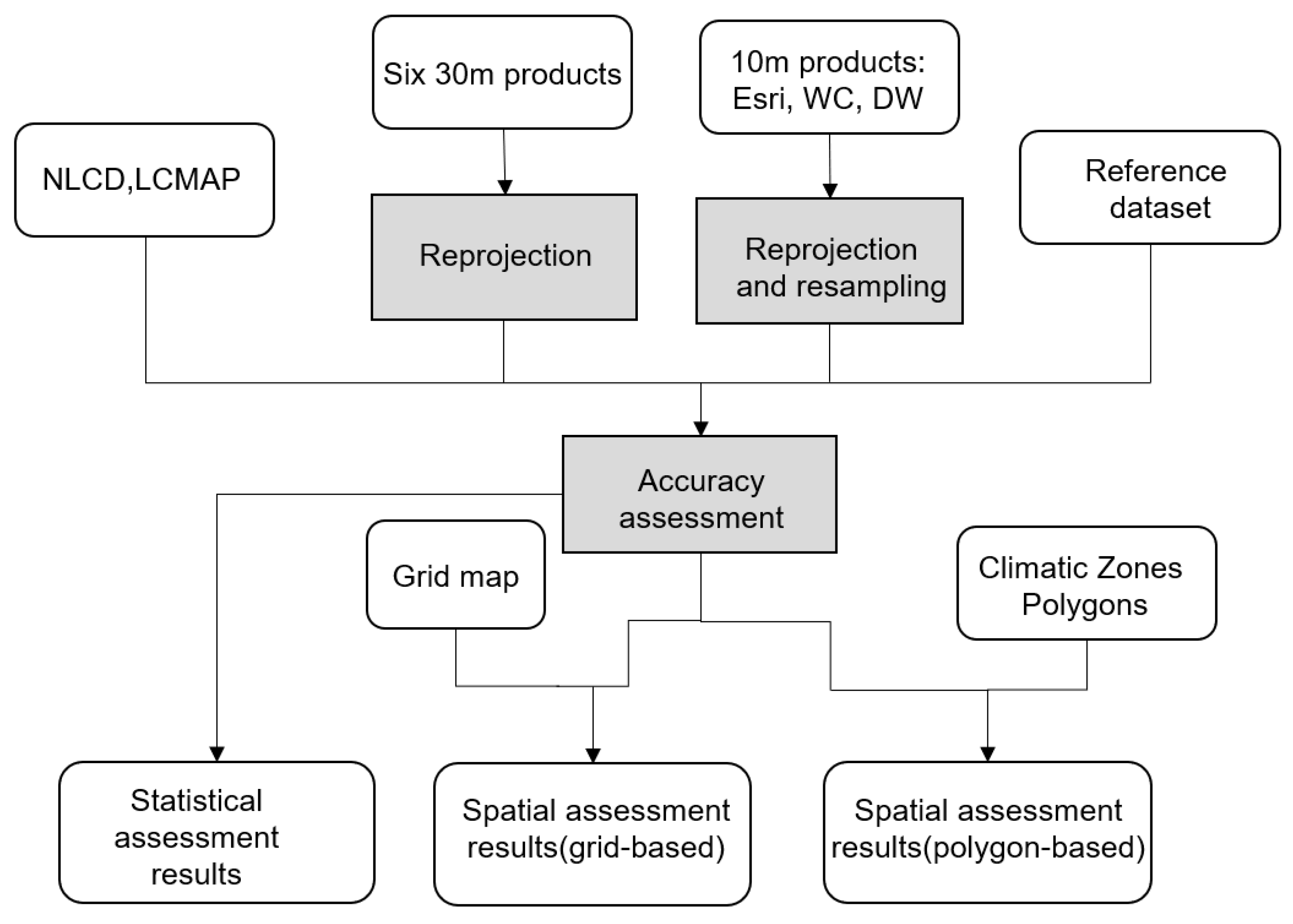
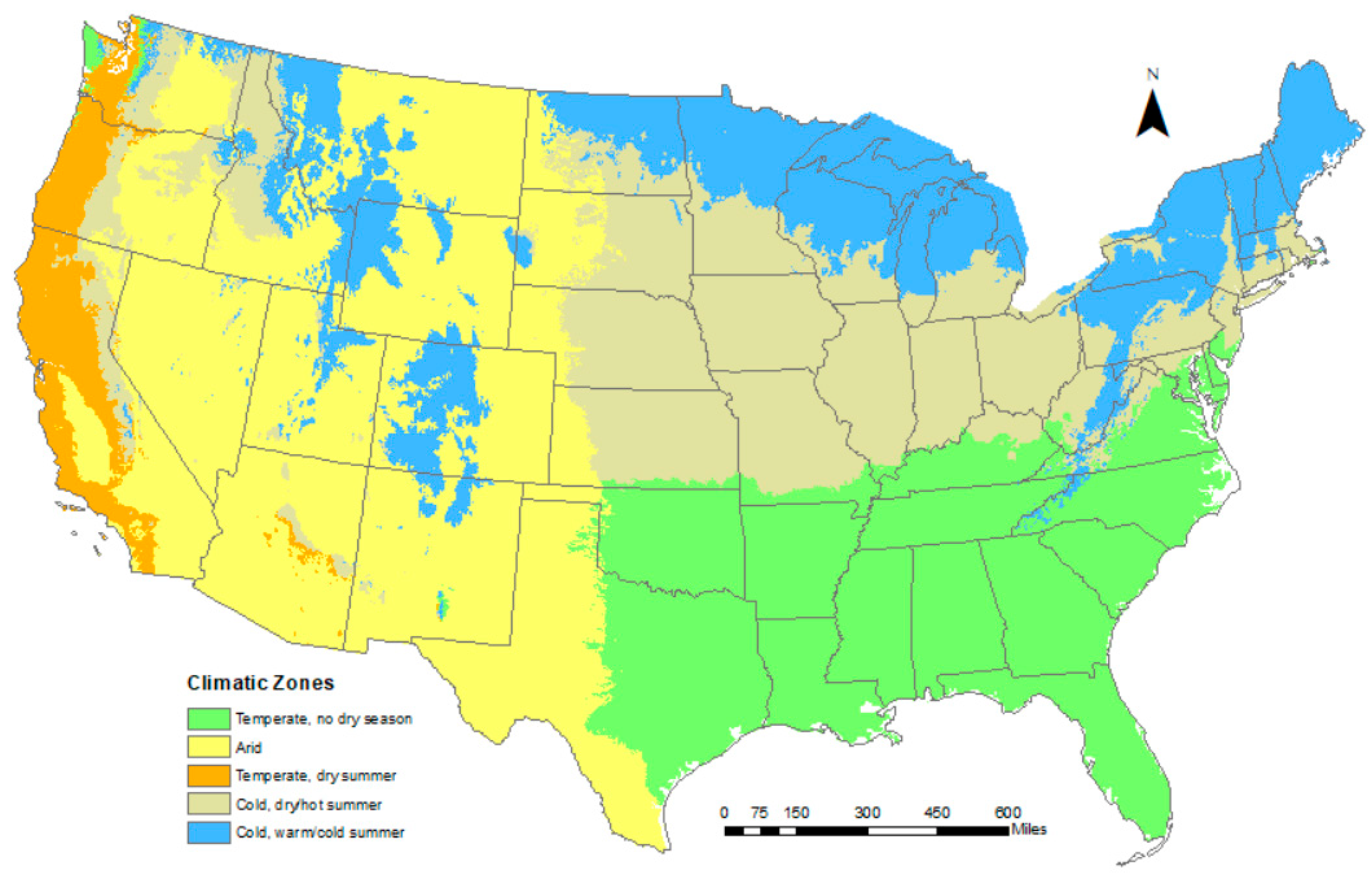
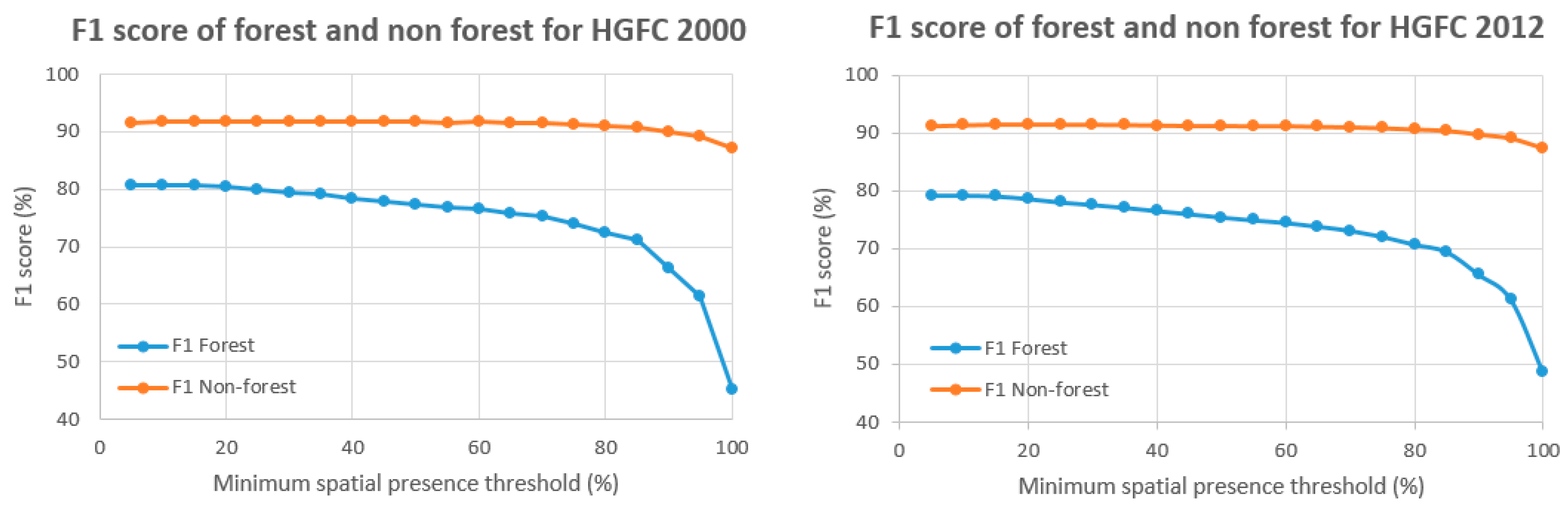
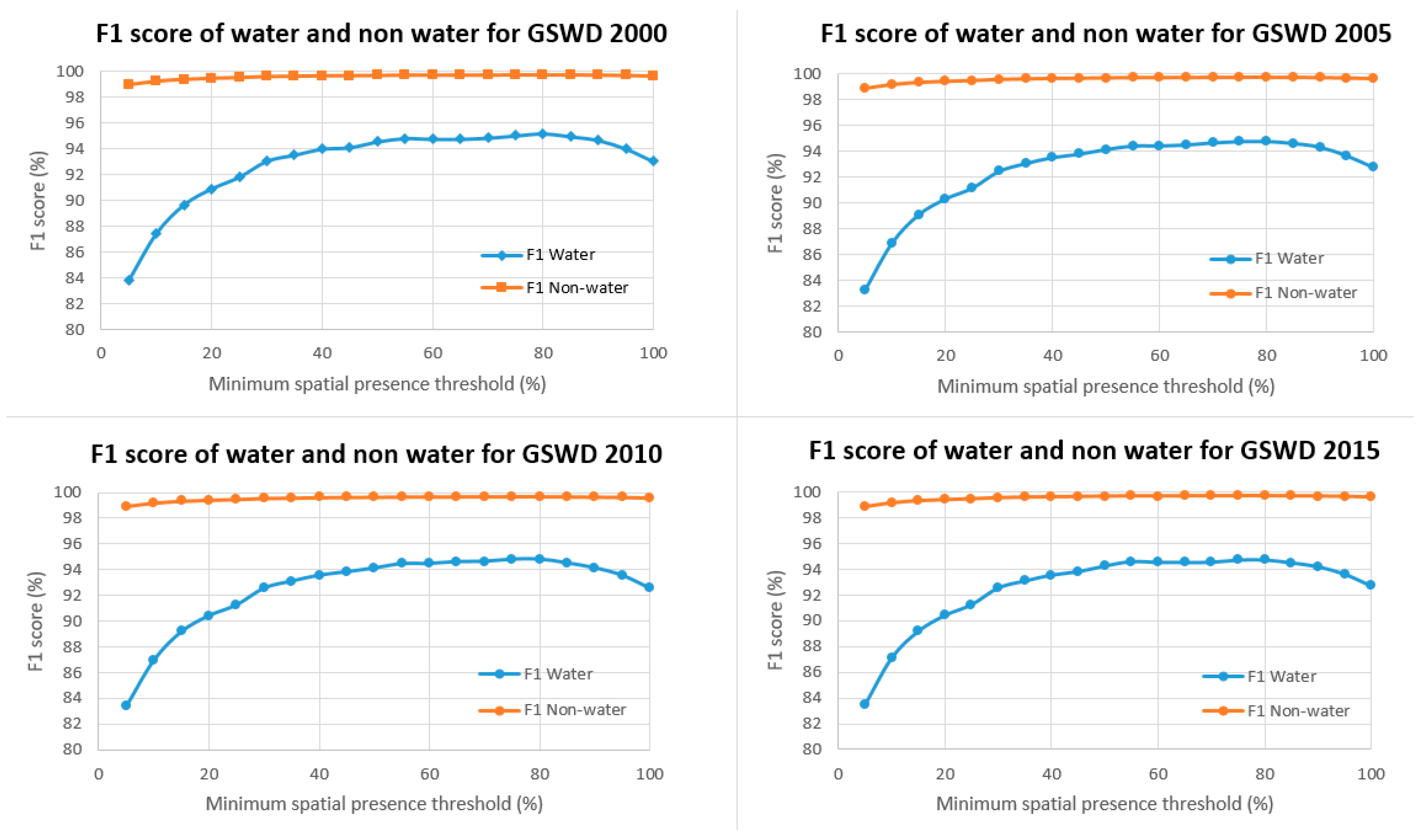
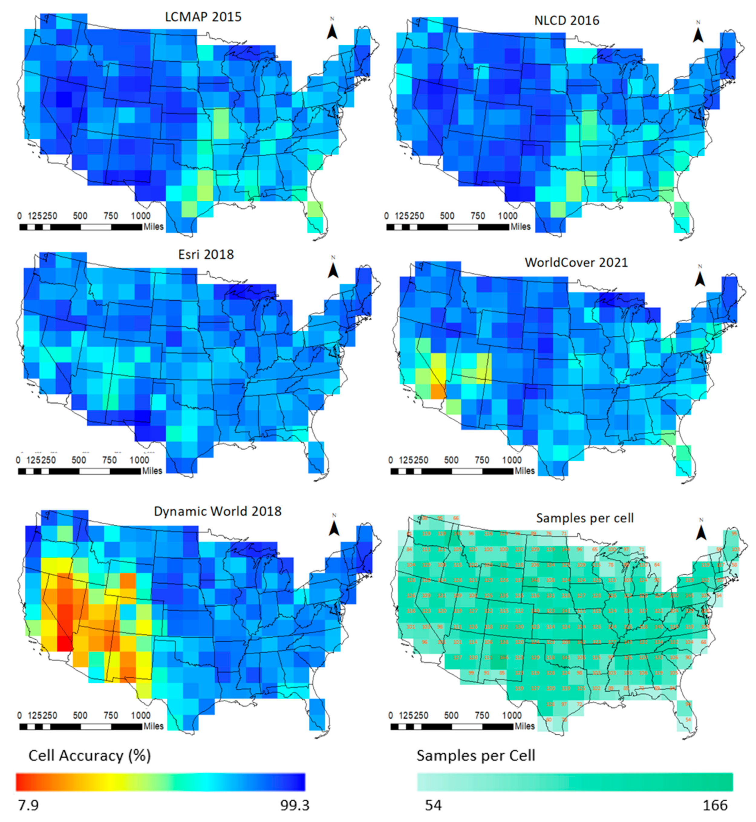
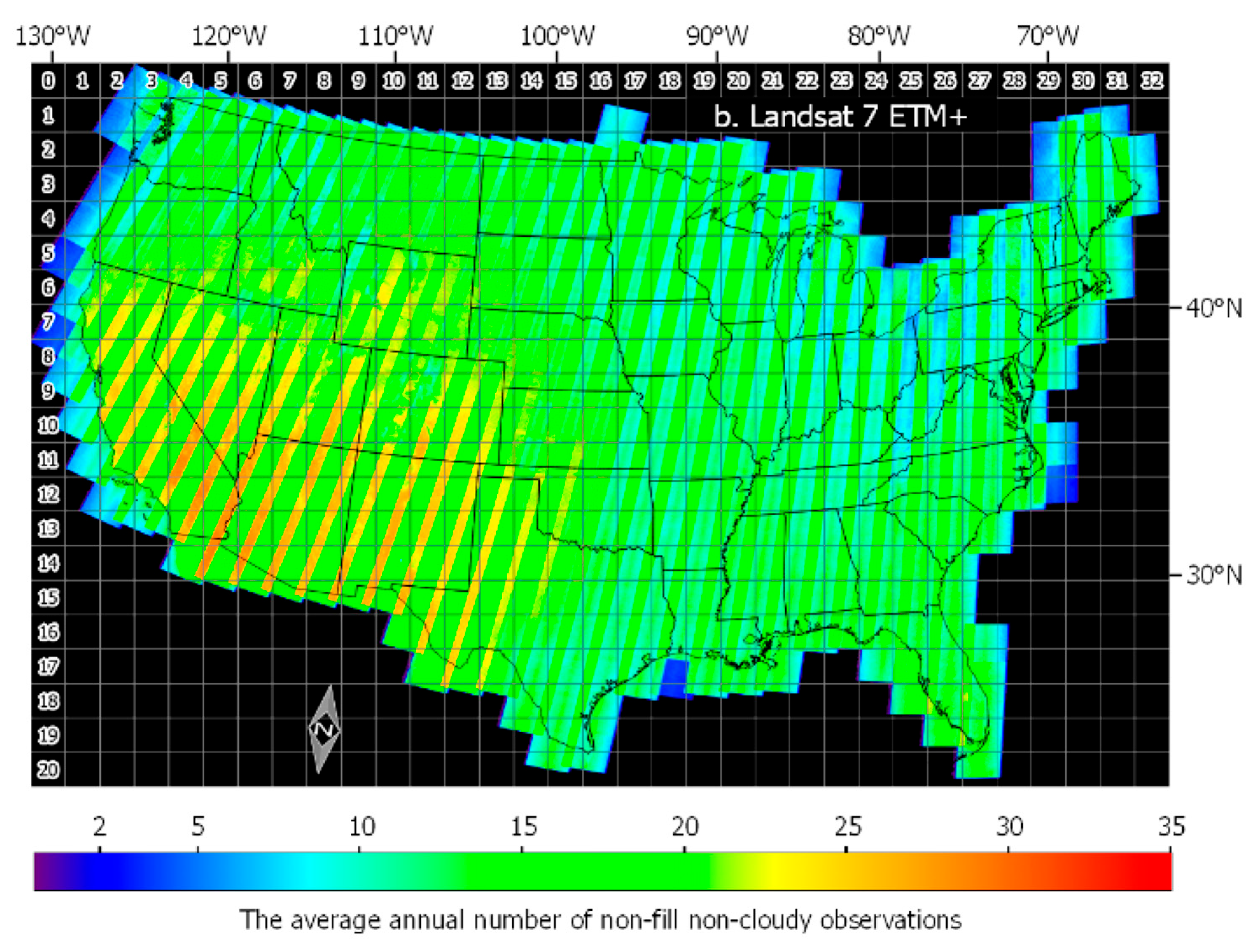
Table A1.
F1 scores for thematic LCLU products over climatic zones.
| Product | Zone | Developed | Cropland | Grass/Shrub | Tree Cover | Water |
|---|---|---|---|---|---|---|
| DW | Temperate, no dry season | 65.6% | 75.3% | 71.6% | 89.4% | 87.8% |
| Arid | 70.1% | 58.1% | 56.3% | 41.6% | 91.8% | |
| Temperate, dry summer | 76.3% | 61.7% | 62.2% | 88.9% | 84.2% | |
| Cold, dry/hot summer | 70.1% | 89.6% | 74.1% | 85.4% | 94.4% | |
| Cold, warm/cold summer | 56.6% | 82.8% | 64.1% | 90.0% | 97.7% | |
| Esri | Temperate, no dry season | 71.3% | 74.9% | 67.1% | 87.5% | 87.0% |
| Arid | 69.9% | 76.7% | 90.0% | 32.0% | 88.1% | |
| Temperate, dry summer | 79.7% | 72.5% | 69.2% | 83.0% | 81.1% | |
| Cold, dry/hot summer | 74.1% | 86.3% | 67.5% | 85.8% | 93.0% | |
| Cold, warm/cold summer | 52.0% | 81.2% | 65.9% | 88.9% | 98.1% | |
| WC | Temperate, no dry season | 30.3% | 77.6% | 67.2% | 86.5% | 84.5% |
| Arid | 56.0% | 82.0% | 85.8% | 71.5% | 88.3% | |
| Temperate, dry summer | 56.6% | 62.7% | 67.9% | 85.3% | 84.8% | |
| Cold, dry/hot summer | 27.7% | 88.2% | 72.7% | 81.8% | 89.9% | |
| Cold, warm/cold summer | 16.7% | 84.3% | 69.8% | 91.3% | 98.0% | |
| LCMAP | Temperate, no dry season | 68.2% | 66.1% | 52.3% | 86.4% | 85.5% |
| Arid | 72.1% | 85.6% | 94.2% | 76.7% | 89.3% | |
| Temperate, dry summer | 82.1% | 79.5% | 72.1% | 84.8% | 87.5% | |
| Cold, dry/hot summer | 72.1% | 85.0% | 68.3% | 87.7% | 93.2% | |
| Cold, warm/cold summer | 50.0% | 78.1% | 64.6% | 90.8% | 97.7% | |
| NLCD | Temperate, no dry season | 73.1% | 67.8% | 53.3% | 84.6% | 89.2% |
| Arid | 67.2% | 88.0% | 94.5% | 74.2% | 89.9% | |
| Temperate, dry summer | 79.0% | 77.7% | 69.0% | 82.9% | 87.5% | |
| Cold, dry/hot summer | 75.2% | 86.0% | 66.8% | 86.7% | 92.0% | |
| Cold, warm/cold summer | 61.5% | 81.6% | 65.3% | 89.5% | 98.6% |
References
- Mueller, R.; Seffrin, R. New methods and satellites: A program update on the NASS cropland data layer acreage program. Intl. Arch. Photogramm. Remote Sens. Spat. Inf. Sci. 2006, 36, 8. [Google Scholar]
- Sellers, P.J.; Tucker, C.J.; Collatz, G.J.; Los, S.; Justice, C.O.; Dazlich, D.A.; Randall, D. A Revised Land Surface Parameterization (SiB2) for Atmospheric GCMS. Part II: The Generation of Global Fields of Terrestrial Biophysical Parameters from Satellite Data. J. Clim. 1996, 9, 706–737. [Google Scholar] [CrossRef]
- Verburg, P.H.; Neumann, K.; Nol, L. Challenges in using land use and land cover data for global change studies. Glob. Chang. Biol. 2011, 17, 974–989. [Google Scholar] [CrossRef] [Green Version]
- Chapin, F.S., 3rd; Zavaleta, E.S.; Eviner, V.T.; Naylor, R.L.; Vitousek, P.M.; Reynolds, H.L.; Hooper, D.U.; Lavorel, S.; Sala, O.E.; Hobbie, S.E.; et al. Consequences of changing biodiversity. Nature 2000, 405, 234–242. [Google Scholar] [CrossRef]
- Luyssaert, S.; Jammet, M.; Stoy, P.C.; Estel, S.; Pongratz, J.; Ceschia, E.; Churkina, G.; Don, A.; Erb, K.; Ferlicoq, M.; et al. Land management and land-cover change have impacts of similar magnitude on surface temperature. Nat. Clim. Chang. 2014, 4, 389–393. [Google Scholar] [CrossRef] [Green Version]
- Loveland, T.R.; Belward, A.S. The IGBP-DIS global 1km land cover data set, DISCover: First results. Int. J. Remote Sens. 1997, 18, 3289–3295. [Google Scholar] [CrossRef]
- Loveland, T.R.; Reed, B.C.; Brown, J.F.; Ohlen, D.O.; Zhu, Z.; Yang, L.; Merchant, J.W. Development of a global land cover characteristics database and IGBP DISCover from 1 km AVHRR data. Int. J. Remote Sens. 2000, 21, 1303–1330. [Google Scholar] [CrossRef]
- Hansen, M.C.; DeFries, R.S.; Townshend, J.R.; Sohlberg, R. Global land cover classification at 1 km spatial resolution using a classification tree approach. Int. J. Remote Sens. 2000, 21, 1331–1364. [Google Scholar] [CrossRef]
- Bartholomé, E.; Belward, A.S. GLC2000: A new approach to global land cover mapping from Earth observation data. Int. J. Remote Sens. 2005, 26, 1959–1977. [Google Scholar] [CrossRef]
- Friedl, M.A.; McIver, D.K.; Hodges, J.C.F.; Zhang, X.Y.; Muchoney, D.; Strahler, A.H.; Woodcock, C.E.; Gopal, S.; Schneider, A.; Cooper, A.; et al. Global land cover mapping from MODIS: Algorithms and early results. Remote Sens. Environ. 2002, 83, 287–302. [Google Scholar] [CrossRef]
- Friedl, M.A.; Sulla-Menashe, D.; Tan, B.; Schneider, A.; Ramankutty, N.; Sibley, A.; Huang, X. MODIS Collection 5 global land cover: Algorithm refinements and characterization of new products. Remote Sens. Environ. 2010, 114, 168–182. [Google Scholar] [CrossRef]
- Tateishi, R.; Hoan, N.T.; Kobayashi, T.; Alsaaideh, B.; Tana, G.; Phong, D.X. Production of global land cover data-GLCNMO2008. J. Geogr. Geol. 2014, 6, 99. [Google Scholar] [CrossRef] [Green Version]
- Arino, O.; Gross, D.; Ranera, F.; Leroy, M.; Bicheron, P.; Brockman, C.; Defourny, P.; Vancutsem, C.; Achard, F.; Weber, J.L. GlobCover: ESA service for global land cover from MERIS. In Proceedings of the 2007 IEEE International Geoscience and Remote Sensing Symposium, Barcelona, Spain, 23–28 July 2007; pp. 2412–2415. [Google Scholar]
- Arino, O.; Perez, J.J.R.; Kalogirou, V.; Bontemps, S.; Defourny, P.; Van Bogaert, E. Global Land Cover Map for 2009 (GlobCover 2009). PANGAEA. Available online: https://doi.pangaea.de/10.1594/PANGAEA.787668 (accessed on 1 January 2014).
- Gong, P.; Wang, J.; Yu, L.; Zhao, Y.; Zhao, Y.; Liang, L.; Chen, J. Finer resolution observation and monitoring of global land cover: First mapping results with Landsat TM and ETM+ data. Int. J. Remote Sens. 2013, 34, 2607–2654. [Google Scholar] [CrossRef] [Green Version]
- Yu, L.; Wang, J.; Gong, P. Improving 30 m global land-cover map FROM-GLC with time series MODIS and auxiliary data sets: A segmentation-based approach. Int. J. Remote Sens. 2013, 34, 5851–5867. [Google Scholar] [CrossRef]
- Chen, J.; Chen, J.; Liao, A.; Cao, X.; Chen, L.; Chen, X.; He, C.; Han, G.; Peng, S.; Lu, M.; et al. Global land cover mapping at 30 m resolution: A POK-based operational approach. ISPRS J. Photogramm. Remote Sens. 2015, 103, 7–27. [Google Scholar] [CrossRef] [Green Version]
- Karra, K.; Kontgis, C.; Statman-Weil, Z.; Mazzariello, J.C.; Mathis, M.; Brumby, S.P. Global land use/land cover with Sentinel 2 and deep learning. In Proceedings of the 2021 IEEE International Geoscience and Remote Sensing Symposium IGARSS, Brussels, Belgium, 11–16 July 2021; pp. 4704–4707. [Google Scholar]
- Zanaga, D.; Van De Kerchove, R.; Daems, D.; De Keersmaecker, W.; Brockmann, C.; Kirches, G.; Wevers, J.; Cartus, O.; Santoro, M.; Fritz, S.; et al. ESA WorldCover 10 m 2021 v200. Available online: https://zenodo.org/record/7254221 (accessed on 1 January 2022).
- Zanaga, D.; Van De Kerchove, R.; De Keersmaecker, W.; Souverijns, N.; Brockmann, C.; Quast, R.; Wevers, J.; Grosu, A.; Paccini, A.; Vergnaud, S.; et al. ESA WorldCover 10 m 2020 V100. OpenAIRE 2021. Available online: https://www.openaire.eu/ (accessed on 30 April 2023).
- Brown, C.F.; Brumby, S.P.; Guzder-Williams, B.; Birch, T.; Hyde, S.B.; Mazzariello, J.; Czerwinski, W.; Pasquarella, V.J.; Haertel, R.; Ilyushchenko, S.; et al. Dynamic World, Near real-time global 10 m land use land cover mapping. Sci. Data 2022, 9, 251. [Google Scholar] [CrossRef]
- Homer, C.; Dewitz, J.; Yang, L.; Jin, S.; Danielson, P.; Xian, G.; Coulston, J.W.; Herold, N.; Wickham, J.D.; Megown, K. Completion of the 2011 National Land Cover Database for the conterminous United States–representing a decade of land cover change information. Photogramm. Eng. Remote Sens. 2015, 81, 345–354. [Google Scholar]
- Healey, S.P.; Cohen, W.B.; Yang, Z.; Brewer, C.K.; Brooks, E.B.; Gorelick, N.; Hernandez, A.J.; Huang, C.; Hughes, M.J.; Kennedy, R.E.; et al. Mapping forest change using stacked generalization: An ensemble approach. Remote Sens. Environ. 2018, 204, 717–728. [Google Scholar] [CrossRef]
- Brown, J.F.; Tollerud, H.J.; Barber, C.P.; Zhou, Q.; Dwyer, J.L.; Vogelmann, J.E.; Loveland, T.R.; Woodcock, C.E.; Stehman, S.V.; Zhu, Z.; et al. Lessons learned implementing an operational continuous United States national land change monitoring capability: The Land Change Monitoring, Assessment, and Projection (LCMAP) approach. Remote Sens. Environ. 2020, 238, 111356. [Google Scholar] [CrossRef]
- Panagos, P.; Meusburger, K.; Ballabio, C.; Borrelli, P.; Alewell, C. Soil erodibility in Europe: A high-resolution product based on LUCAS. Sci. Total Environ. 2014, 479, 189–200. [Google Scholar] [CrossRef] [PubMed]
- Yang, Y.; Xiao, P.; Feng, X.; Li, H. Accuracy assessment of seven global land cover datasets over China. ISPRS J. Photogramm. Remote Sens. 2017, 125, 156–173. [Google Scholar] [CrossRef]
- Herold, M.; Mayaux, P.; Woodcock, C.E.; Baccini, A.; Schmullius, C. Some challenges in global land cover mapping: An assessment of agreement and accuracy in existing 1 km products. Remote Sens. Environ. 2008, 112, 2538–2556. [Google Scholar] [CrossRef]
- Bai, Y.; Feng, M.; Jiang, H.; Wang, J.; Zhu, Y.; Liu, Y. Assessing Consistency of Five Global Land Cover Data Sets in China. Remote Sens. 2014, 6, 8739–8759. [Google Scholar] [CrossRef] [Green Version]
- Tsendbazar, N.; de Bruin, S.; Mora, B.; Schouten, L.; Herold, M. Comparative assessment of thematic accuracy of GLC maps for specific applications using existing reference data. Int. J. Appl. Earth Obs. Geoinf. 2016, 44, 124–135. [Google Scholar] [CrossRef]
- Liang, L.; Liu, Q.; Liu, G.; Li, H.; Huang, C. Accuracy Evaluation and Consistency Analysis of Four Global Land Cover Products in the Arctic Region. Remote Sens. 2019, 11, 1396. [Google Scholar] [CrossRef] [Green Version]
- Gao, Y.; Liu, L.; Zhang, X.; Chen, X.; Mi, J.; Xie, S. Consistency analysis and accuracy assessment of three global 30-m land-cover products over the European Union using the LUCAS product. Remote Sens. 2020, 12, 3479. [Google Scholar] [CrossRef]
- Zhang, C.; Dong, J.; Ge, Q. Quantifying the accuracies of six 30-m cropland products over China: A comparison and evaluation analysis. Comput. Electron. Agric. 2022, 197, 106946. [Google Scholar] [CrossRef]
- Pengra, B.W.; Stehman, S.V.; Horton, J.A.; Dockter, D.J.; Schroeder, T.A.; Yang, Z.; Hernandez, A.J.; Healey, S.P.; Cohen, W.B.; Finco, M.V.; et al. LCMAP Reference Data Product 1984–2018 Land Cover, Land Use and Change Process Attributes (ver. 1.2, November 2021): U.S. Geological Survey Data Release; U.S. Geological Survey: Reston, VA, USA, 2020. [Google Scholar] [CrossRef]
- Stehman, S.V.; Pengra, B.W.; Horton, J.A.; Wellington, D.F. Validation of the US Geological Survey’s Land Change Monitoring, Assessment and Projection (LCMAP) Collection 1.0 annual land cover products 1985–2017. Remote Sens. Environ. 2021, 265, 112646. [Google Scholar] [CrossRef]
- U.S. Geological Survey. Joint Response Design for TimeSync Reference Data Collection; U.S. Geological Survey: Sioux Falls, SD, USA, 2019. Available online: www.usgs.gov/media/files/joint-response-design-timesync-reference-data-collection (accessed on 30 July 2021).
- Cohen, W.B.; Yang, Z.; Kennedy, R. Detecting trends in forest disturbance and recovery using yearly Landsat time series: 2. TimeSync—Tools for calibration and validation. Remote Sens. Environ. 2010, 114, 2911–2924. [Google Scholar] [CrossRef]
- Pengra, B.W.; Stehman, S.V.; Horton, J.A.; Dockter, D.J.; Schroeder, T.A.; Yang, Z.; Cohen, W.B.; Healey, S.P.; Loveland, T.R. Quality control and assessment of interpreter consistency of annual land cover reference data in an operational national monitoring program. Remote Sens. Environ. 2020, 238, 111261. [Google Scholar] [CrossRef]
- Czaplewski, R.L. Accuracy assessment of maps of forest condition: Statistical design and methodological considerations. In Remote Sensing of Forest Environments: Concepts and Case Studies; Springer: New York, NY, USA, 2003; pp. 115–140. [Google Scholar]
- Yu, L.; Du, Z.; Dong, R.; Zheng, J.; Tu, Y.; Chen, X.; Hao, P.; Zhong, B.; Peng, D.; Gong, P. FROM-GLC Plus: Toward near real-time and multi-resolution land cover mapping. GIScience Remote Sens. 2022, 59, 1026–1047. [Google Scholar] [CrossRef]
- Brovelli, M.A.; Molinari, M.E.; Hussein, E.; Chen, J.; Li, R. The First Comprehensive Accuracy Assessment of GlobeLand30 at a National Level: Methodology and Results. Remote Sens. 2015, 7, 4191–4212. [Google Scholar] [CrossRef] [Green Version]
- Han, G.; Chen, J.; He, C.; Li, S.; Wu, H.; Liao, A.; Peng, S. A web-based system for supporting global land cover data production. ISPRS J. Photogramm. Remote Sens. 2015, 103, 66–80. [Google Scholar] [CrossRef]
- Chen, J.; Cao, X.; Peng, S.; Ren, H. Analysis and Applications of GlobeLand30: A Review. ISPRS Int. J. Geo-Inf. 2017, 6, 230. [Google Scholar] [CrossRef] [Green Version]
- Pickens, A.H.; Hansen, M.C.; Hancher, M.; Stehman, S.V.; Tyukavina, A.; Potapov, P.; Marroquin, B.; Sherani, Z. Mapping and sampling to characterize global inland water dynamics from 1999 to 2018 with full Landsat time-series. Remote Sens. Environ. 2020, 243, 111792. [Google Scholar] [CrossRef]
- Liu, L.; Zhang, X.; Gao, Y.; Chen, X.; Shuai, X.; Mi, J. Finer-resolution mapping of global land cover: Recent developments, consistency analysis, and prospects. J. Remote Sens. 2021, 2021, 5289697. [Google Scholar] [CrossRef]
- Gong, P.; Li, X.; Wang, J.; Bai, Y.; Chen, B.; Hu, T.; Liu, X.; Xu, B.; Yang, J.; Zhang, W.; et al. Annual maps of global artificial impervious area (GAIA) between 1985 and 2018. Remote Sens. Environ. 2020, 236, 111510. [Google Scholar] [CrossRef]
- Hansen, M.C.; Potapov, P.V.; Moore, R.; Hancher, M.; Turubanova, S.A.; Tyukavina, A.; Thau, D.; Stehman, S.V.; Goetz, S.J.; Loveland, T.R.; et al. High-Resolution Global Maps of 21st-Century Forest Cover Change. Science 2013, 342, 850–853. [Google Scholar] [CrossRef] [Green Version]
- Vogelmann, J.E.; Howard, S.M.; Yang, L.; Larson, C.R.; Wylie, B.K.; Van Driel, N. Completion of the 1990s Na-tional Land Cover Data Set for the conterminous United States from Landsat Thematic Mapper data and ancillary data sources. Photogramm. Eng. Remote Sens. 2001, 67, 6. [Google Scholar]
- Anderson, J.R. A Land Use and Land Cover Classification System for Use with Remote Sensor Data (Vol. 964); US Government Printing Office: Washington, DC, USA, 1976. [Google Scholar]
- Fry, J.; Coan, M.; Homer, C.G.; Meyer, D.K.; Wickham, J. Completion of the National Land Cover Database (NLCD) 1992–2001 Land Cover Change Retrofit Product; U.S. Geological Survey: Reston, VA, USA, 2008. [Google Scholar] [CrossRef]
- Wickham, J.; Stehman, S.; Fry, J.; Smith, J.; Homer, C. Thematic accuracy of the NLCD 2001 land cover for the conterminous United States. Remote Sens. Environ. 2010, 114, 1286–1296. [Google Scholar] [CrossRef]
- Wickham, J.D.; Stehman, S.V.; Gass, L.; Dewitz, J.; Fry, J.A.; Wade, T.G. Accuracy assessment of NLCD 2006 land cover and impervious surface. Remote Sens. Environ. 2013, 130, 294–304. [Google Scholar] [CrossRef]
- Wickham, J.; Stehman, S.V.; Gass, L.; Dewitz, J.A.; Sorenson, D.G.; Granneman, B.J.; Poss, R.V.; Baer, L.A. Thematic accuracy assessment of the 2011 National Land Cover Database (NLCD). Remote Sens. Environ. 2017, 191, 328–341. [Google Scholar] [CrossRef] [Green Version]
- Wickham, J.; Stehman, S.V.; Sorenson, D.G.; Gass, L.; Dewitz, J.A. Thematic accuracy assessment of the NLCD 2016 land cover for the conterminous United States. Remote Sens. Environ. 2021, 257, 112357. [Google Scholar] [CrossRef]
- Dwyer, J.L.; Roy, D.P.; Sauer, B.; Jenkerson, C.B.; Zhang, H.K.; Lymburner, L. Analysis Ready Data: Enabling Analysis of the Landsat Archive. Remote Sens. 2018, 10, 1363. [Google Scholar] [CrossRef]
- Zhu, Z.; Woodcock, C.E. Continuous change detection and classification of land cover using all available Landsat data. Remote Sens. Environ. 2014, 144, 152–171. [Google Scholar] [CrossRef] [Green Version]
- Boryan, C.; Yang, Z.; Mueller, R.; Craig, M. Monitoring US agriculture: The US Department of Agriculture, National Agricultural Statistics Service, Cropland Data Layer Program. Geocarto Int. 2011, 26, 341–358. [Google Scholar] [CrossRef]
- Boryan, C.G.; Yang, Z. Deriving crop specific covariate data sets from multi-year NASS geospatial cropland data layers. In Proceedings of the 2013 IEEE International Geoscience and Remote Sensing Symposium—IGARSS, Melbourne, Australia, 21–26 July 2013; pp. 4225–4228. [Google Scholar] [CrossRef] [Green Version]
- Xian, G.Z.; Smith, K.; Wellington, D.; Horton, J.; Zhou, Q.; Li, C.; Auch, R.; Brown, J.F.; Zhu, Z.; Reker, R.R. Implementation of the CCDC algorithm to produce the LCMAP Collection 1.0 annual land surface change product. Earth Syst. Sci. Data 2022, 14, 143–162. [Google Scholar] [CrossRef]
- Brown, J.F. LCMAP Collection 1.1 Science Product Guide. 2022. Available online: https://www.usgs.gov/media/files/lcmap-science-product-guide (accessed on 9 February 2022).
- Brown, J.F. LSDS-1424 LCMAP Data Format Control Book (DFCB). 2022. Available online: https://www.usgs.gov/media/files/lcmap-dfcb (accessed on 9 February 2022).
- Czaplewski, R.L. Misclassification bias in areal estimates. Photogramm. Eng. Remote Sens. 1992, 58, 189–192. [Google Scholar]
- Muller, S.V.; Walker, D.A.; Nelson, F.E.; Auerback, N.A.; Bockheim, J.G.; Guyer, S.; Sherba, D. Accuracy as-sessment of a land-cover map of the Kuparuk river basin, Alaska: Considerations for remote regions. Photogramm. Eng. Remote Sens. 1998, 64, 619–628. [Google Scholar]
- Stehman, S.V. Selecting and interpreting measures of thematic classification accuracy. Remote Sens. Environ. 1997, 62, 77–89. [Google Scholar] [CrossRef]
- Todd, W.J.; Gehring, D.G.; Haman, J.F. Landsat wildland mapping accuracy. Photogramm. Eng. Remote Sens. 1980, 46, 509–520. [Google Scholar]
- Scepan, J. Thematic validation of high-resolution global land-cover data sets. Photogramm. Eng. Remote Sens. 1999, 65, 1051–1060. [Google Scholar]
- Loveland, T.R.; Zhu, Z.; Ohlen, D.O.; Brown, J.F.; Reed, B.C.; Yang, L. An analysis of the IGBP global land-cover characterization process. Photogramm. Eng. Remote Sens. 1999, 65, 1021–1032. [Google Scholar]
- Latifovic, R.; Olthof, I. Accuracy assessment using sub-pixel fractional error matrices of global land cover products derived from satellite data. Remote Sens. Environ. 2004, 90, 153–165. [Google Scholar] [CrossRef]
- Wang, L.; Bartlett, P.; Pouliot, D.; Chan, E.; Lamarche, C.; Wulder, M.A.; Defourny, P.; Brady, M. Comparison and Assessment of Regional and Global Land Cover Products for Use in CLASS over Canada. Remote Sens. 2019, 11, 2286. [Google Scholar] [CrossRef] [Green Version]
- Beck, H.E.; Zimmermann, N.E.; McVicar, T.R.; Vergopolan, N.; Berg, A.; Wood, E.F. Present and future Kö-ppen-Geiger climate classification maps at 1-km resolution. Sci. Data 2018, 5, 1–12. [Google Scholar] [CrossRef] [PubMed] [Green Version]
- Venter, Z.S.; Barton, D.N.; Chakraborty, T.; Simensen, T.; Singh, G. Global 10 m Land Use Land Cover Datasets: A Comparison of Dynamic World, World Cover and Esri Land Cover. Remote Sens. 2022, 14, 4101. [Google Scholar] [CrossRef]
- Wickham, J.; Stehman, S.; Smith, J.; Yang, L. Thematic accuracy of the 1992 National Land-Cover Data for the western United States. Remote Sens. Environ. 2004, 91, 452–468. [Google Scholar] [CrossRef]
- OpenStreetMap contributors. Planet Dump. 2020. Available online: https://planet.openstreetmap.org (accessed on 30 April 2023).
- Pekel, J.-F.; Cottam, A.; Gorelick, N.; Belward, A.S. High-resolution mapping of global surface water and its long-term changes. Nature 2016, 540, 418–422. [Google Scholar] [CrossRef]
- Bunting, P.; Rosenqvist, A.; Lucas, R.M.; Rebelo, L.M.; Hilarides, L.; Thomas, N.; Hardy, A.; Itoh, T.; Shimada, M.; Finlayson, C.M. The Global Mangrove Watch—A New 2010 Global Baseline of Mangrove Extent. Remote Sens. 2018, 10, 1669. [Google Scholar] [CrossRef] [Green Version]
- Corbane, C.; Sabo, F.; Politis, P.; Syrris, V. GHS-BUILT-S2 R2020A-GHS Built-Up Grid, Derived from Sentinel-2 Global Image Composite for Reference Year 2018 using Convolutional Neural Networks (GHS-S2Net); European Commission, Joint Research Centre (JRC): Brussels, Belgium, 2020. [Google Scholar]
- Chauhan, N.K.; Singh, K. A review on conventional machine learning vs. deep learning. In Proceedings of the 2018 International Conference on Computing, Power and Communication Technologies, GUCON 2018, Greater Noida, India, 28–29 September 2018; pp. 347–352. [Google Scholar] [CrossRef]
- Wang, P.; Fan, E.; Wang, P. Comparative analysis of image classification algorithms based on traditional machine learning and deep learning. Pattern Recognit. Lett. 2021, 141, 61–67. [Google Scholar] [CrossRef]
- Egorov, A.V.; Roy, D.P.; Zhang, H.K.; Li, Z.; Yan, L.; Huang, H. Landsat 4, 5 and 7 (1982 to 2017) Analysis Ready Data (ARD) Observation Coverage over the Conterminous United States and Implications for Terrestrial Monitoring. Remote Sens. 2019, 11, 447. [Google Scholar] [CrossRef] [Green Version]
Figure 1.
Workflow for statistical and spatial accuracy assessments. Six 30 m products are GlobeLand30, FROM-GLC, GSWD, GAIA, HGFC and CDL.
Figure 1.
Workflow for statistical and spatial accuracy assessments. Six 30 m products are GlobeLand30, FROM-GLC, GSWD, GAIA, HGFC and CDL.

Figure 2.
Five climatic zones for the conterminous United States.

Figure 3.
F1 score of HGFC with thresholds for year 2000 (left) and 2012 (right).

Figure 4.
F1 score of GSWD with different thresholds for years from 2000 to 2015.

Figure 5.
Spatial agreement percentage maps of LCMAP, NLCD, ESRI, World Cover and Dynamic World for recent years using developed, cropland, grass/shrub, tree cover and water classes.
Figure 5.
Spatial agreement percentage maps of LCMAP, NLCD, ESRI, World Cover and Dynamic World for recent years using developed, cropland, grass/shrub, tree cover and water classes.

Figure 6.
The average annual number of non-fill non-cloudy observations at each CONUS ARD 30 m pixel location over the 36-year study period (1982–2017) for Landsat 7 ETM+. Adapted from Figure 6 of [78].

Table 1.
Global mapping products.
| Product | Time | Resolution | Reference |
|---|---|---|---|
| IGBP DISCover | 1992–1993 | 1 km | [6,7] |
| UMD | 1992–1993 | 1 km | [8] |
| GLC | 2000 | 1 km | [9] |
| MODIS LC | 2001–2013 | 500/1000 m | [10,11] |
| GLCNMO | 2003/2008 | 500 m | [12] |
| GlobCover | 2005/2006/2009 | 300 m | [13,14] |
| FROM-GLC | 2010/2015/2017 | 30 m | [15,16] |
| GlobeLand30 | 2000/2010 | 30 m | [17] |
| Esri | 2017–2021 | 10 m | [18] |
| WC | 2020/2021 | 10 m | [19,20] |
| DW | 2015–2023 | 10 m | [21] |
Table 2.
Sample number per class for the overall reference dataset and the spatial edge samples.
| Samples | Developed | Cropland | Grass/Shrub | Tree Cover | Water | Wetland | Barren |
|---|---|---|---|---|---|---|---|
| All | 1372 | 4363 | 9491 | 6980 | 1333 | 1241 | 217 |
| Spatial edge | 688 | 919 | 1789 | 2361 | 147 | 414 | 62 |
Table 3.
Summary of the eleven LCLU products included in this study.
| Products | Esri | WC | DW | GlobeLand30 | FROMGLC | NLCD | LCMAP | HGFC | GSWD | GAIA | CDL |
|---|---|---|---|---|---|---|---|---|---|---|---|
| Sensor | Sentinel 2 | Sentinel 1/2 | Sentinel 2 | Landsat TM/ETM+, HJ-1 | Landsat TM, ETM+, OLI | Landsat TM, ETM+, OLI | Landsat TM, ETM+, OLI | Landsat TM, ETM+, OLI | Landsat TM, ETM+, OLI | Landsat TM, ETM+, OLI | Landsat TM, ETM+ OLI, AWiFS, MODIS |
| Spatial resolution | 10 m | 10 m | 10 m | 30 m | 30 m | 30 m | 30 m | 30 m | 30 m | 30 m | 30 m |
| Spatial extent | Global | Global | Global | Global | Global | US-only | US-only | Global | Global | Global | US-only |
| Available Years | Annual 2017–2021 | 2020, 2021 | Annual 2015–2022 | 2000, 2010 | 2010, 2015, 2017 | 92,200-1 4,6,8,11,13,16,19 | Annual 1985–2021 | Annual 2000–2021 | Annual 1999–2018 | Annual 1985–2018 | Annual 1997–2021 |
| Included Years | 2018 | 2020, 2021 | 2018 | 2000,2010 | 2010, 2015 | 1992, 2001, 2011, 2016 | 1990, 1995, 2000, 2005,2010,2015 | 2000, 2012 | 2000, 2005, 2010, 2015 | 1990, 2000, 2010, 2015 | 2010, 2015 |
| Multi/Single-Class | Multi | Multi | Multi | Multi | Multi | Multi | Multi | Single | Single | Single | Single |
| Classes | 9 | 11 | 9 | 10 | A unique land cover classification scheme | Anderson Level II | Anderson Level I | Percent + binary for gain and loss | Percent | binary | 255 |
| Classifier | AI | RF | AI | Pixel- and object-based | Various | DT | CCDC | DT | Tree-based | Google Earth Engine | DT |
| Reference | [18] | [19] | [21] | [42] | [15] | [52] | [34] | [46] | [43] | [44] | [56] |
Note: AI = Artificial Intelligence method, RF = Random Forest, DT = Decision Tree, CCDC = Continuous Change Detection and Classification, Various = MLC, DT, RF and SVM, MLC = Maximum Likelihood Classifier, SVM = Support Vector Machine.
Table 4.
Conversion table of classification schemes of LCLU products and potential issues.
| LCMAP | NLCD | FROM-GLC | GlobeLand30 | Esri | Dynamic World | World Cover |
|---|---|---|---|---|---|---|
| Developed | Developed | Impervious | Artificial surfaces | Built Area | Built Area | Built-up Urban green such as parks not included |
| Cropland | Planted/Cultivated | Cropland; Orchards * Fruit trees not included, classified as forests (except for orchards) | Cultivated land | Crops Crops at tree height not included (e.g., fruit trees) | Crops Crops at tree height not included (e.g., fruit trees) | Cropland Perennial woody crops and greenhouses not included |
| Grass/Shrub | Shrubland; Herbaceous 20% vs. 10% LCMAP threshold | Grasslands; Shrublands; Tundra ^ | Grassland; Shrubland; Tundra | Rangeland ^ | Grass; Shrub/Scrub ^ Parks, golf courses, baseball included but LCMAP assigns them as Developed | Grassland; Shrubland; Moss and Lichen |
| Tree cover | Forest 20% vs. 10% LCMAP threshold | Broadleaf; Needleleaf; Mixed Forest ^* | Forest | Trees Dense tall vegetation in swamps or mangroves included | Trees ^ Dense tall vegetation in swamps or mangroves, fruit trees included | Tree cover Prioritizes trees, includes trees present with other classes (built-up, woody crops, flooded trees) |
| Water | Open Water * | Waterbodies | Water bodies | Water | Water | Permanent waterbodies |
| Wetland | Wetlands | Wetlands Forest wetland not included | Wetland | Flooded vegetation Swamp forests not included, includes heavily irrigated and inundated agriculture | Flooded vegetation Swamp forests not included | Herbaceous Wetland; Mangroves Swamp forests not included |
| Barren | Barren 15% vs. 10% LCMAP threshold | Barren land ^ Lake/river bottoms in dry season included | Bare land Saline/Alkaline land included | Bare ground ^ Dried lake beds, mines included | Bare ground ^ Dried lake bottoms, mines, large empty urban lots, dirt roads included | Bare/sparse vegetation |
Note: ^ Minimum spatial presence not provided; * Level II Class; Cells in grey do not allow comparisons as class definitions deviate substantially between product and reference.
Table 5.
Climate zones and corresponding class code.
| # | Group Description | Corresponding Köppen–Geiger Class Code |
|---|---|---|
| 1 | Temperate, no dry season | 1, 2, 3, 14, 15, 16 |
| 2 | Arid | 4, 5, 6, 7 |
| 3 | Temperate, dry summer | 8, 9, 10 |
| 4 | Cold, dry/hot summer | 17, 18, 19, 21, 22, 25 |
| 5 | Cold, warm/cold summer | 26, 27, 29 |
Table 6.
F1 scores for LCLU products (gray cells are not comparable due to varying class definitions).
Table 6.
F1 scores for LCLU products (gray cells are not comparable due to varying class definitions).
| Products | F1 Score | ||||||
|---|---|---|---|---|---|---|---|
| Developed | Cropland | Grass/Shrub | Tree Cover | Water | Wetland | Barren | |
| NLCD 1992 | 49.3% | 73.2% | 78.8% | 81.0% | 92.1% | 62.6% | 27.7% |
| NLCD 2001 | 70.3% | 79.8% | 83.4% | 86.0% | 95.6% | 77.0% | 55.1% |
| NLCD 2011 | 72.1% | 80.7% | 83.4% | 85.2% | 95.4% | 76.9% | 56.4% |
| NLCD 2016 | 72.1% | 81.2% | 83.6% | 85.0% | 95.5% | 76.9% | 56.2% |
| LCMAP 1990 | 68.2% | 80.2% | 83.6% | 87.0% | 94.6% | 71.5% | 47.2% |
| LCMAP 1995 | 69.4% | 80.3% | 83.9% | 87.2% | 94.5% | 71.5% | 48.5% |
| LCMAP 2000 | 70.1% | 80.3% | 84.0% | 86.9% | 94.6% | 71.8% | 48.2% |
| LCMAP 2005 | 70.1% | 79.6% | 83.9% | 86.6% | 94.2% | 70.9% | 49.5% |
| LCMAP 2010 | 69.8% | 79.2% | 83.6% | 86.4% | 94.3% | 71.2% | 50.0% |
| LCMAP 2015 | 69.5% | 79.1% | 83.4% | 85.9% | 94.4% | 71.1% | 50.1% |
| FROMGLC 2010 | 4.8% | 35.5% | 24.8% | 63.2% | 81.4% | 5.5% | 7.4% |
| FROMGLC 2015 | 45.3% | 63.3% | 68.9% | 77.6% | 91.1% | 3.3% | 16.5% |
| GlobeLand30 2000 | 54.5% | 76.4% | 79.6% | 80.4% | 76.1% | 63.4% | 35.7% |
| GlobeLand30 2010 | 56.2% | 75.8% | 79.5% | 79.5% | 76.0% | 62.9% | 37.2% |
| Esri 2018 | 70.8% | 80.7% | 80.8% | 78.7% | 94.5% | 11.7% | 49.5% |
| WC 2020 | 33.1% | 86.3% | 80.8% | 83.0% | 95.5% | 18.2% | 25.2% |
| WC 2021 | 34.1% | 84.0% | 78.9% | 80.1% | 94.3% | 17.1% | 27.6% |
| DW 2018 | 67.6% | 77.0% | 61.5% | 79.7% | 94.9% | 8.0% | 13.2% |
Table 7.
User’s and Producer’s Accuracy for comparable classes of LCLU products (Wetland and Barren are excluded).
Table 7.
User’s and Producer’s Accuracy for comparable classes of LCLU products (Wetland and Barren are excluded).
| User’s Accuracy | Producer’s Accuracy | |||||||||
|---|---|---|---|---|---|---|---|---|---|---|
| Developed | Cropland | Grass/Shrub | Tree Cover | Water | Developed | Cropland | Grass/Shrub | Tree Cover | Water | |
| NLCD 1992 | 74.6% | 62.5% | 85.4% | 81.2% | 92.7% | 36.8% | 88.3% | 73.1% | 80.8% | 91.5% |
| NLCD 2001 | 67.8% | 71.0% | 87.2% | 92.0% | 96.7% | 73.1% | 91.2% | 79.9% | 80.8% | 94.5% |
| NLCD 2011 | 71.2% | 71.1% | 86.4% | 92.5% | 96.2% | 73.1% | 93.3% | 80.6% | 79.0% | 94.5% |
| NLCD 2016 | 71.7% | 71.9% | 86.4% | 92.0% | 97.1% | 72.6% | 93.3% | 80.9% | 78.9% | 93.8% |
| LCMAP 1990 | 72.1% | 70.6% | 88.4% | 90.1% | 95.9% | 64.6% | 92.7% | 79.3% | 84.1% | 93.3% |
| LCMAP 1995 | 75.5% | 70.3% | 88.7% | 90.1% | 96.1% | 64.2% | 93.6% | 79.5% | 84.5% | 92.9% |
| LCMAP 2000 | 79.4% | 70.0% | 88.2% | 90.4% | 96.7% | 62.7% | 94.1% | 80.2% | 83.7% | 92.5% |
| LCMAP 2005 | 81.2% | 68.9% | 87.7% | 90.5% | 96.1% | 61.7% | 94.2% | 80.3% | 83.1% | 92.5% |
| LCMAP 2010 | 80.7% | 68.5% | 87.1% | 90.6% | 96.5% | 61.5% | 93.7% | 80.3% | 82.6% | 92.3% |
| LCMAP 2015 | 83.1% | 68.4% | 86.8% | 90.1% | 96.8% | 59.7% | 93.9% | 80.2% | 82.1% | 92.1% |
| FROMGLC 2010 | 38.2% | 44.5% | 60.0% | 57.6% | 80.0% | 2.5% | 29.6% | 15.6% | 70.0% | 82.7% |
| FROMGLC 2015 | 91.6% | 70.4% | 68.1% | 72.5% | 90.6% | 30.1% | 57.4% | 69.8% | 83.5% | 91.5% |
| GlobeLand30 2000 | 74.7% | 64.8% | 82.7% | 83.9% | 95.4% | 42.9% | 93.0% | 76.7% | 77.1% | 63.3% |
| GlobeLand30 2010 | 80.6% | 63.6% | 82.3% | 82.7% | 95.7% | 43.1% | 93.7% | 76.8% | 76.6% | 63.0% |
| Esri 2018 | 77.0% | 74.2% | 78.9% | 79.2% | 95.0% | 65.5% | 88.3% | 82.8% | 78.2% | 94.1% |
| WC 2020 | 92.7% | 89.0% | 79.7% | 72.0% | 96.0% | 20.9% | 79.4% | 78.0% | 91.6% | 92.6% |
| WC 2021 | 97.9% | 90.8% | 81.8% | 74.6% | 97.7% | 19.9% | 82.2% | 79.8% | 93.5% | 93.3% |
| DW 2018 | 90.5% | 70.9% | 76.4% | 73.8% | 93.8% | 53.9% | 84.2% | 51.5% | 86.7% | 96.0% |
Table 8.
F1 scores of LCLU products using spatial edge reference samples.
| Products | F1 Score | ||||||
|---|---|---|---|---|---|---|---|
| Developed | Cropland | Grass/Shrub | Tree Cover | Water | Wetland | Barren | |
| NLCD 1992 | 22.8% | 51.4% | 50.2% | 70.1% | 62.7% | 35.4% | 19.0% |
| NLCD 2001 | 57.5% | 55.9% | 51.8% | 74.4% | 70.6% | 58.3% | 45.9% |
| NLCD 2011 | 58.8% | 55.6% | 52.7% | 72.6% | 68.8% | 58.3% | 46.4% |
| NLCD 2016 | 59.3% | 56.0% | 51.6% | 71.3% | 66.9% | 57.9% | 46.3% |
| LCMAP 1990 | 53.2% | 61.2% | 59.3% | 77.6% | 60.6% | 47.9% | 47.1% |
| LCMAP 1995 | 54.1% | 60.4% | 58.7% | 77.5% | 59.8% | 47.8% | 45.2% |
| LCMAP 2000 | 53.7% | 59.1% | 58.1% | 76.6% | 62.5% | 48.2% | 48.7% |
| LCMAP 2005 | 53.0% | 57.1% | 57.6% | 76.2% | 59.1% | 47.0% | 45.8% |
| LCMAP 2010 | 52.9% | 55.7% | 57.3% | 75.4% | 60.7% | 47.3% | 47.1% |
| LCMAP 2015 | 52.0% | 54.9% | 56.3% | 74.6% | 60.3% | 47.2% | 47.4% |
| FROMGLC 2010 | 1.5% | 26.9% | 19.0% | 60.1% | 37.7% | 3.3% | 14.9% |
| FROMGLC 2015 | 18.1% | 41.9% | 52.7% | 70.5% | 52.4% | 0.5% | 31.7% |
| Globeland30 2000 | 24.2% | 52.0% | 50.2% | 66.7% | 50.0% | 31.9% | 31.3% |
| Globeland30 2010 | 26.4% | 49.1% | 49.4% | 65.0% | 49.1% | 30.7% | 31.1% |
| Esri 2018 | 57.0% | 61.6% | 59.5% | 72.0% | 67.1% | 9.7% | 55.2% |
| WC 2020 | 17.8% | 69.3% | 63.7% | 78.3% | 66.9% | 8.4% | 32.0% |
| WC 2021 | 16.6% | 60.1% | 57.6% | 74.1% | 57.5% | 7.5% | 40.3% |
| DW 2018 | 50.7% | 64.7% | 53.4% | 74.6% | 72.3% | 7.5% | 32.4% |
Table 9.
F1 scores difference between spatial edge reference samples and non-edge samples.
| Products | F1 Score | ||||||
|---|---|---|---|---|---|---|---|
| Developed | Cropland | Grass/Shrub | Tree Cover | Water | Wetland | Barren | |
| NLCD 1992 | −51.34% | −29.78% | −34.64% | −16.70% | −32.69% | −40.41% | −12.52% |
| NLCD 2001 | −31.95% | −31.34% | −38.13% | −17.58% | −27.88% | −29.80% | −14.73% |
| NLCD 2011 | −32.62% | −32.47% | −37.25% | −18.96% | −29.76% | −29.67% | −15.84% |
| NLCD 2016 | −31.54% | −32.60% | −38.82% | −20.48% | −31.79% | −30.42% | −15.51% |
| LCMAP 1990 | −31.92% | −25.43% | −29.66% | −14.33% | −37.34% | −36.35% | −0.15% |
| LCMAP 1995 | −32.89% | −26.54% | −30.66% | −14.73% | −38.37% | −36.52% | −4.80% |
| LCMAP 2000 | −35.19% | −28.29% | −31.53% | −15.71% | −35.67% | −36.27% | 0.72% |
| LCMAP 2005 | −36.16% | −29.91% | −31.89% | −15.93% | −38.98% | −36.86% | −5.36% |
| LCMAP 2010 | −36.40% | −31.10% | −32.01% | −16.70% | −37.46% | −36.76% | −4.20% |
| LCMAP 2015 | −37.25% | −32.06% | −32.96% | −17.07% | −36.87% | −36.82% | −3.90% |
| FROMGLC 2010 | −7.20% | −11.54% | −7.17% | −4.72% | −48.76% | −3.24% | 8.87% |
| FROMGLC 2015 | −53.37% | −27.12% | −20.77% | −10.86% | −42.73% | −4.16% | 17.41% |
| Globeland30 2000 | −57.98% | −33.25% | −36.08% | −20.82% | −29.13% | −46.60% | −6.31% |
| Globeland30 2010 | −57.40% | −36.14% | −36.85% | −22.19% | −30.07% | −47.24% | −8.55% |
| Esri 2018 | −30.33% | −24.61% | −26.04% | −10.41% | −31.06% | −2.91% | 7.74% |
| WC 2020 | −32.45% | −20.89% | −21.28% | −7.46% | −31.66% | −14.22% | 8.80% |
| WC 2021 | −36.72% | −29.35% | −26.55% | −10.27% | −40.93% | −13.97% | 15.77% |
| DW 2018 | −35.07% | −15.21% | −10.11% | −8.16% | −25.71% | −0.74% | 21.67% |
Table 10.
Summary of F1 scores for GAIA and CDL products.
| Single-Class Maps | F1_score_class | User’s Accuracy | Producer’s Accuracy |
|---|---|---|---|
| GAIA 1990 | 40.0% | 87.4% | 25.9% |
| GAIA 2000 | 44.5% | 89.1% | 29.7% |
| GAIA 2010 | 46.6% | 89.7% | 31.5% |
| GAIA 2015 | 49.2% | 88.6% | 34.0% |
| CDL 2010 | 61.2% | 65.1% | 57.8% |
| CDL 2015 | 62.8% | 65.8% | 60.0% |
Table 11.
Confusion table for GAIA and CDL products (NC = Non-Class, C = Class).
| GAIA 1990 | GAIA 2000 | GAIA 2010 | GAIA 2015 | CDL 2010 | CDL 2015 | |||||||
|---|---|---|---|---|---|---|---|---|---|---|---|---|
| NC | C | NC | C | NC | C | NC | C | NC | C | NC | C | |
| NC | 23910 | 38 | 23744 | 43 | 23583 | 48 | 23534 | 60 | 19353 | 1329 | 19242 | 1361 |
| C | 754 | 264 | 829 | 350 | 915 | 420 | 905 | 467 | 1808 | 2476 | 1745 | 2618 |
Table 12.
F1 score for LULC products by climatic zones using developed, cropland, grass/shrub, tree cover and water classes.
Table 12.
F1 score for LULC products by climatic zones using developed, cropland, grass/shrub, tree cover and water classes.
| Products | Average F1 Score of Developed, Cropland, Grass/Shrub, Tree and Water | ||||
| Temperate, No Dry Season | Arid | Temperate, Dry Summer | Cold, Dry/Hot Summer | Cold, Warm/Cold Summer | |
| LCMAP 2015 | 71.7% | 83.6% | 81.2% | 81.2% | 76.3% |
| NLCD 2016 | 73.6% | 82.8% | 79.2% | 81.4% | 79.3% |
| ESRI 2018 | 77.6% | 71.3% | 77.1% | 81.3% | 77.2% |
| WC 2021 | 69.2% | 76.7% | 71.5% | 72.1% | 72.0% |
| DW 2018 | 77.9% | 63.6% | 74.7% | 82.7% | 78.2% |
| Samples | 5213 | 8035 | 860 | 5409 | 3524 |
| Samples/1000 km2 | 2.79 | 2.99 | 2.82 | 3.01 | 2.75 |
Disclaimer/Publisher’s Note: The statements, opinions and data contained in all publications are solely those of the individual author(s) and contributor(s) and not of MDPI and/or the editor(s). MDPI and/or the editor(s) disclaim responsibility for any injury to people or property resulting from any ideas, methods, instructions or products referred to in the content. |
© 2023 by the authors. Licensee MDPI, Basel, Switzerland. This article is an open access article distributed under the terms and conditions of the Creative Commons Attribution (CC BY) license (https://creativecommons.org/licenses/by/4.0/).
Share and Cite
MDPI and ACS Style
Wang, Z.; Mountrakis, G. Accuracy Assessment of Eleven Medium Resolution Global and Regional Land Cover Land Use Products: A Case Study over the Conterminous United States. Remote Sens. 2023, 15, 3186. https://doi.org/10.3390/rs15123186
AMA Style
Wang Z, Mountrakis G. Accuracy Assessment of Eleven Medium Resolution Global and Regional Land Cover Land Use Products: A Case Study over the Conterminous United States. Remote Sensing. 2023; 15(12):3186. https://doi.org/10.3390/rs15123186
Chicago/Turabian StyleWang, Zhixin, and Giorgos Mountrakis. 2023. "Accuracy Assessment of Eleven Medium Resolution Global and Regional Land Cover Land Use Products: A Case Study over the Conterminous United States" Remote Sensing 15, no. 12: 3186. https://doi.org/10.3390/rs15123186
Note that from the first issue of 2016, this journal uses article numbers instead of page numbers. See further details here.