
A New Blind Selection Approach for Lunar Landing Zones Based on Engineering Constraints Using Sliding Window
 ,
,  , ,
, ,  and
and
Abstract
:1. Introduction
2. Materials and Methods
2.1. LOLA Data Introduction and Pre-Processing
2.2. Methods
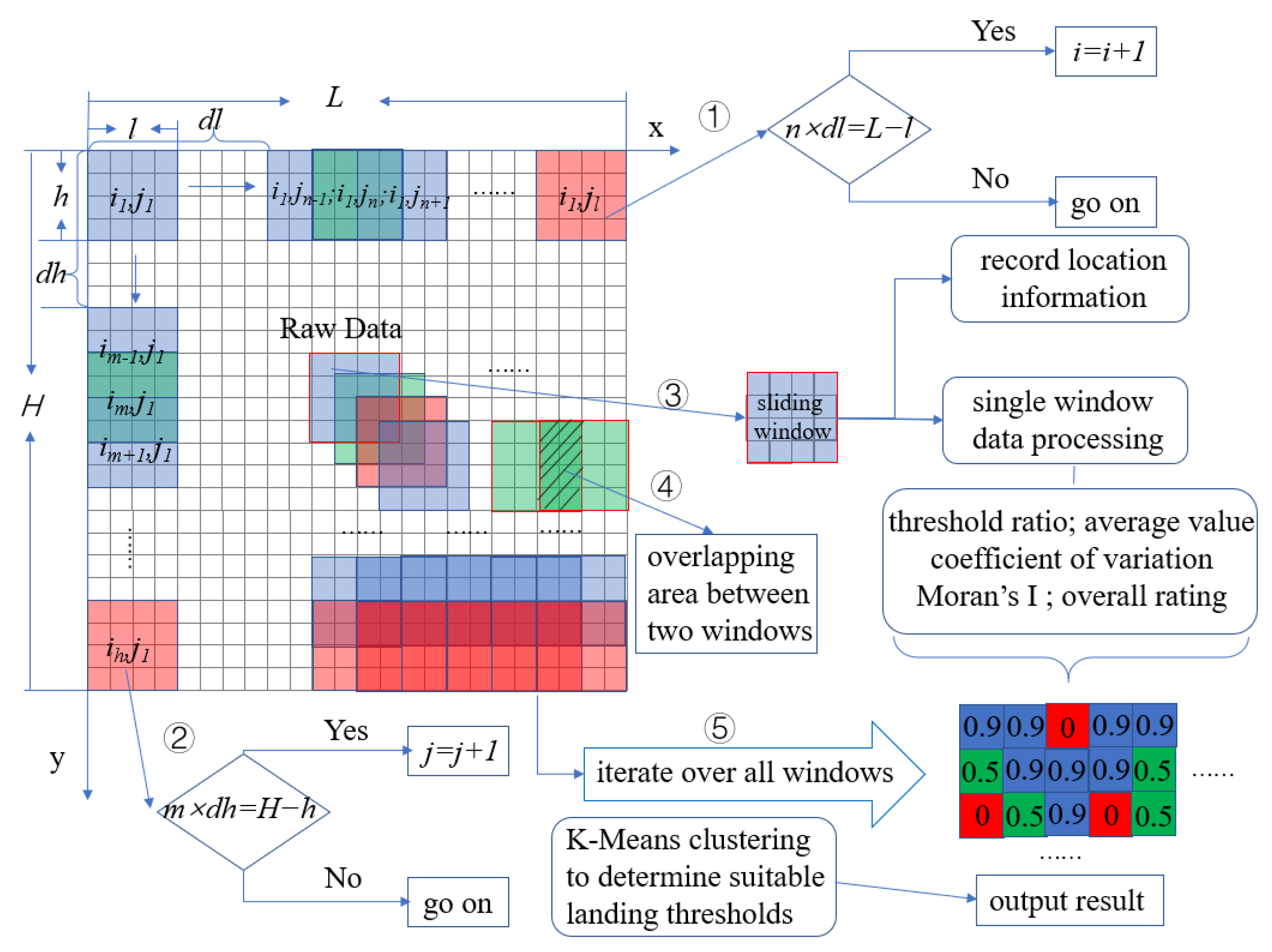
2.2.1. The Sliding Window Principle
- Selecting the window size: The first step in using sliding windows is to select the window size that contains the number of data points in each window, depending on the specific problem to be solved and the properties of the data set. During the landing zone selection process, the choice of window size depends mainly on the purpose of the landing site. For example, if the purpose is to build a lunar base, a larger area is needed to accommodate the site selection; if the purpose is for a lander landing, the smaller the window size, the better with high-resolution data.
- Window slide: Once the window size is selected, the window begins to slide into the dataset within a specified increment. The distance between each slide is called the step size and determines the degree of overlap between successive windows. This is shown in Figure 3 ④.
- Sliding termination condition: When sliding lengthwise, as in Figure 3 ①, the window slides from the beginning of the next line if the product of the column index and lengthwise step is equal to the difference between the data length and the window length; correspondingly, when sliding widthwise, the decision condition is as in Figure 3 ②. If both ① and ② are satisfied, it means that the traversal cycle of the original data is complete, and the sliding is terminated.
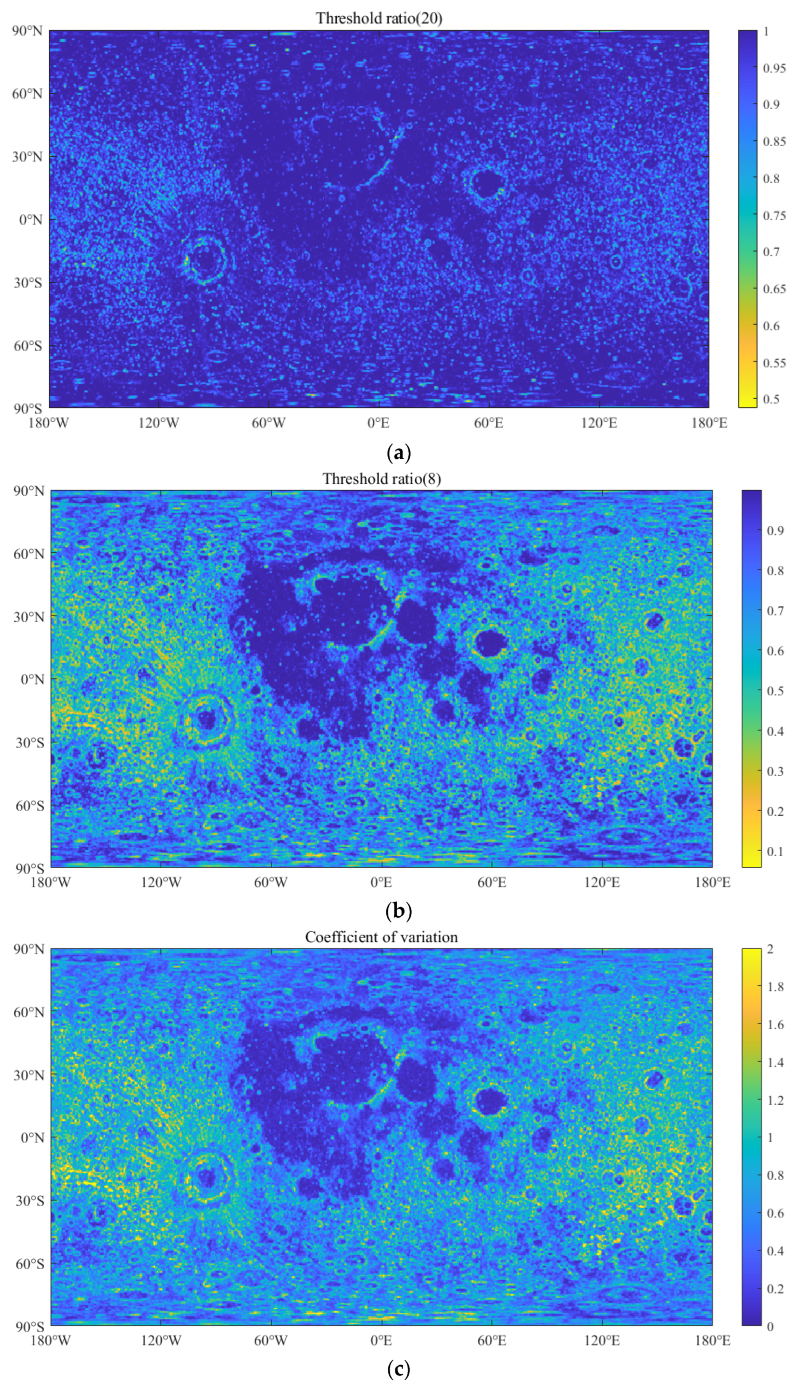
- Data analysis: As the windows move through the data set, each window is analyzed independently. Independent analysis of the windows includes recording the window position information and processing the data from each window. Data processing includes statistics and the calculation of the average slope, threshold ratio, coefficient of variation, Moran’s I, and overall rating.
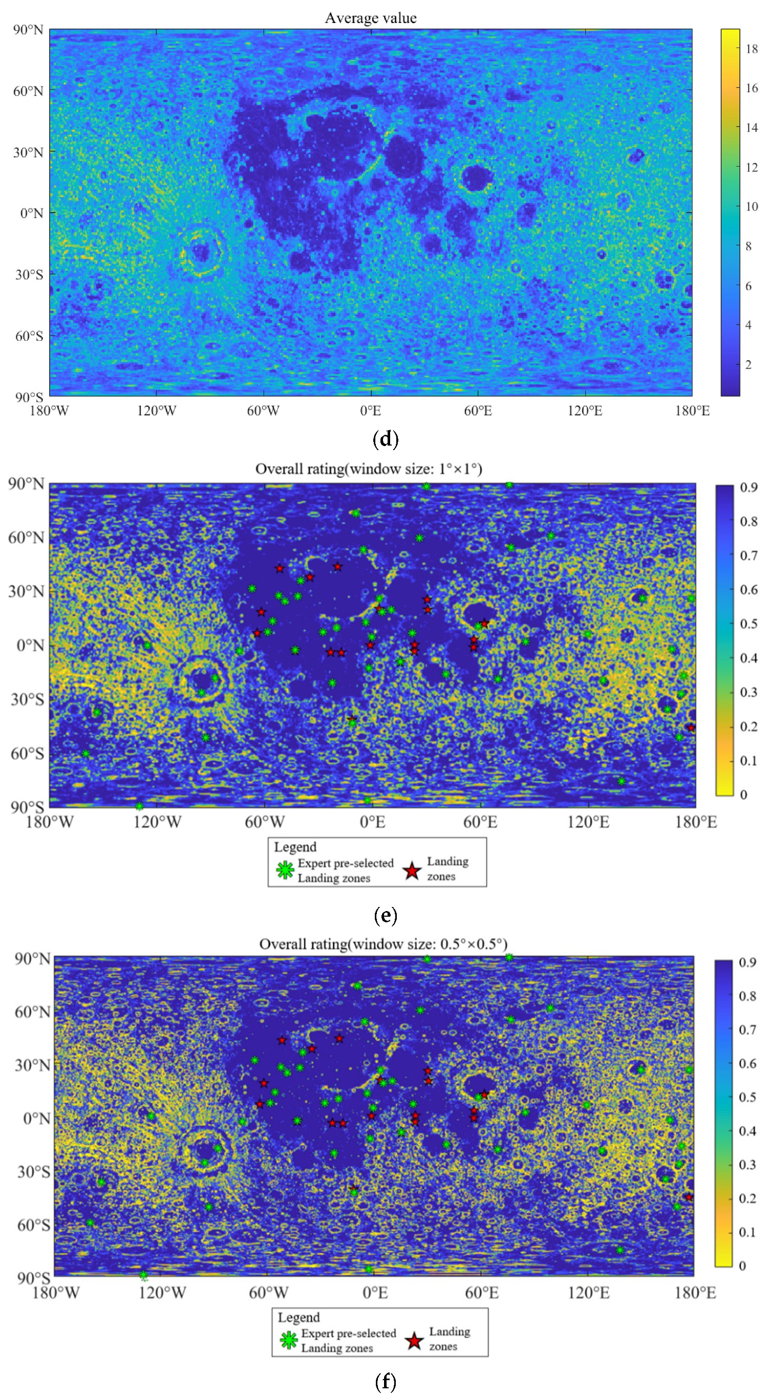
- Output generation: When the sliding of the original data is completed, as shown in Figure 3 ⑤, each window already contains the corresponding index, which results in the output. The output results represent the summary statistics of each window, or a set of features extracted from the slope data, to generate the landing zone selection results in the form of a matrix or surface elements. “Surface elements” means the area corresponding to the window size is contained in surface elements. For example, the attributes of a 1° × 1° window size include the composite indicator within the window as well as the 30.3 × 30.3 km2 area and range filled by that window. In the rendering process, a k-means clustering algorithm is used to determine the appropriate thresholds for landing.
2.2.2. Threshold Ratio
2.2.3. The Coefficient of Variation
2.2.4. Moran Index
2.2.5. Overall Rating and Factor Weights
2.2.6. K-Means Clustering Algorithm
3. Results
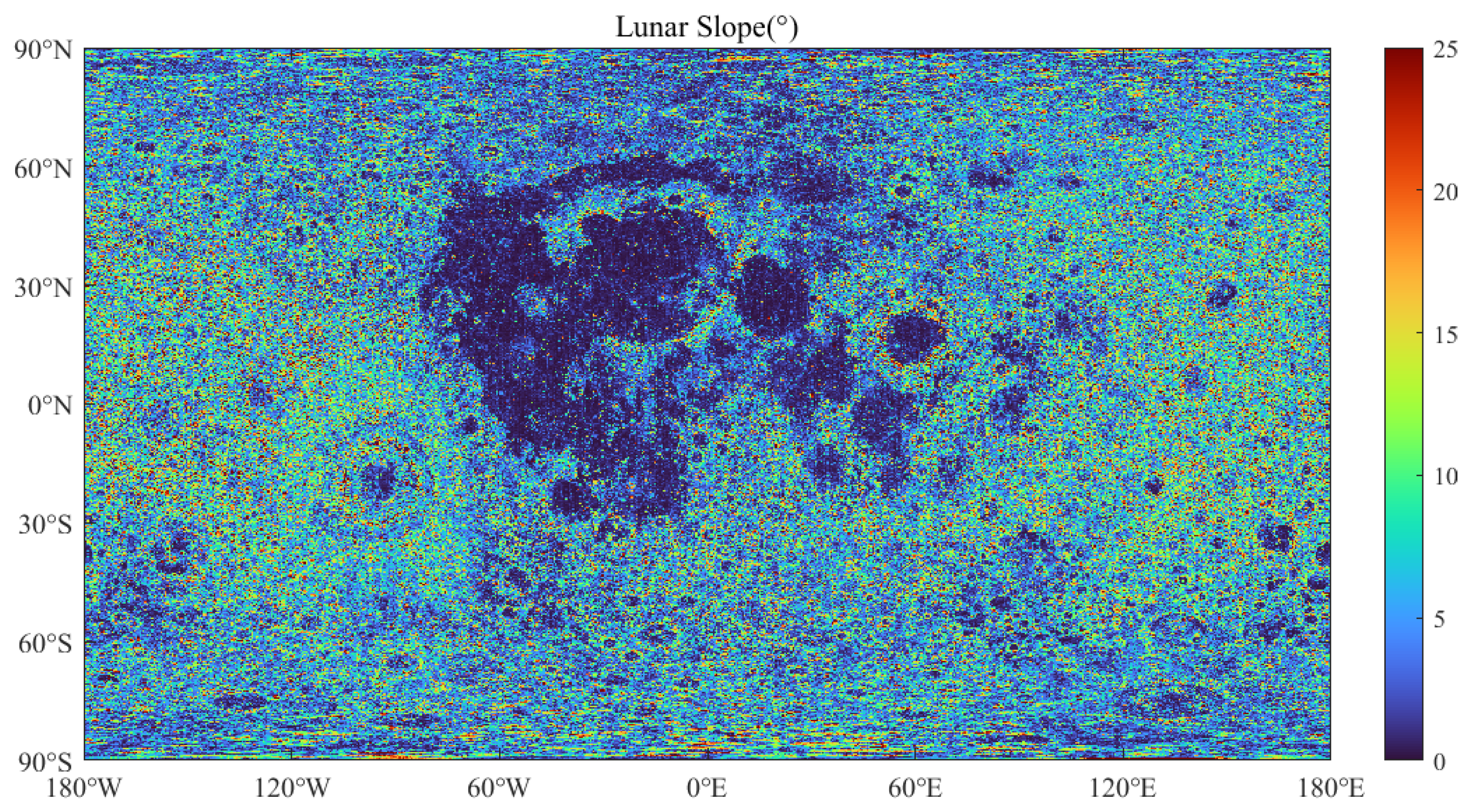
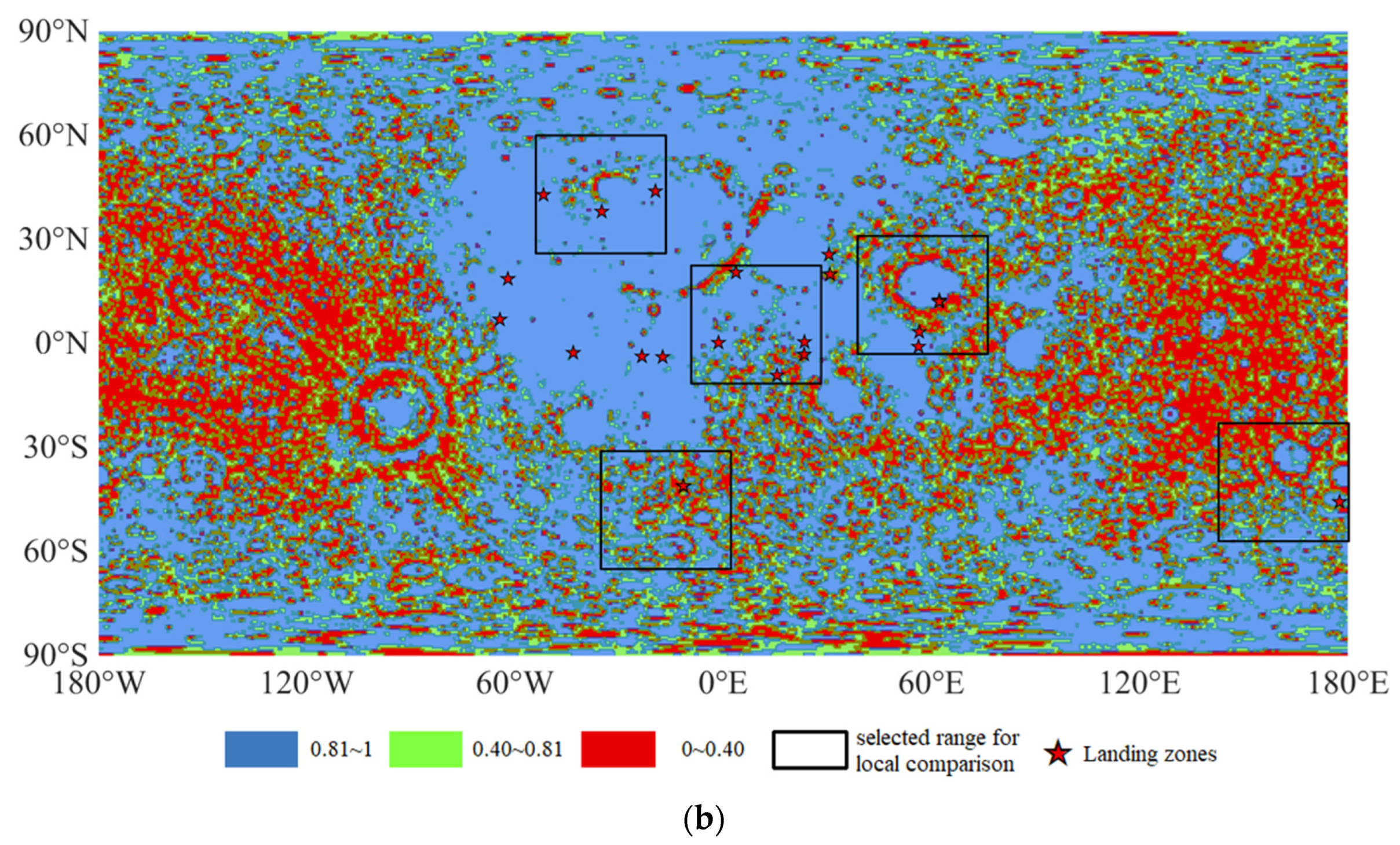
3.1. Quantitative Results of Whole Moon Slope Evaluation
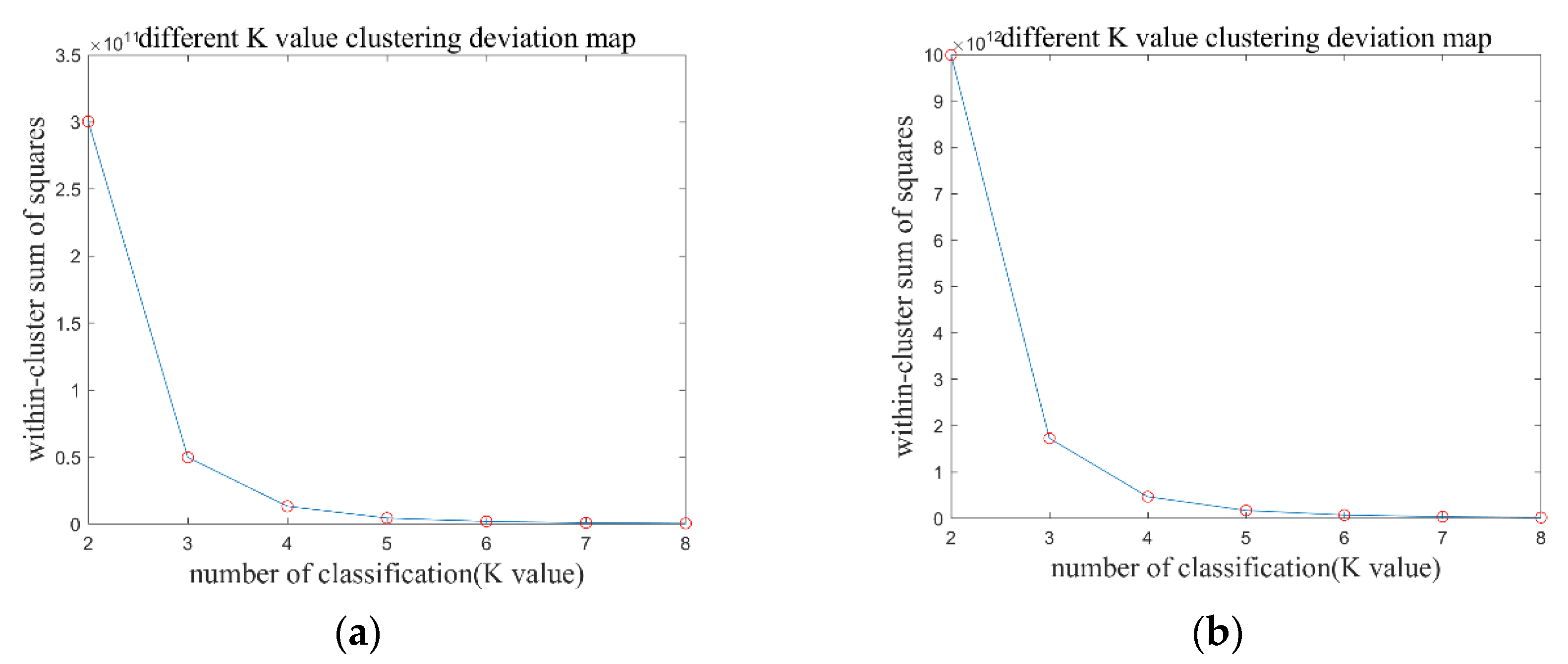
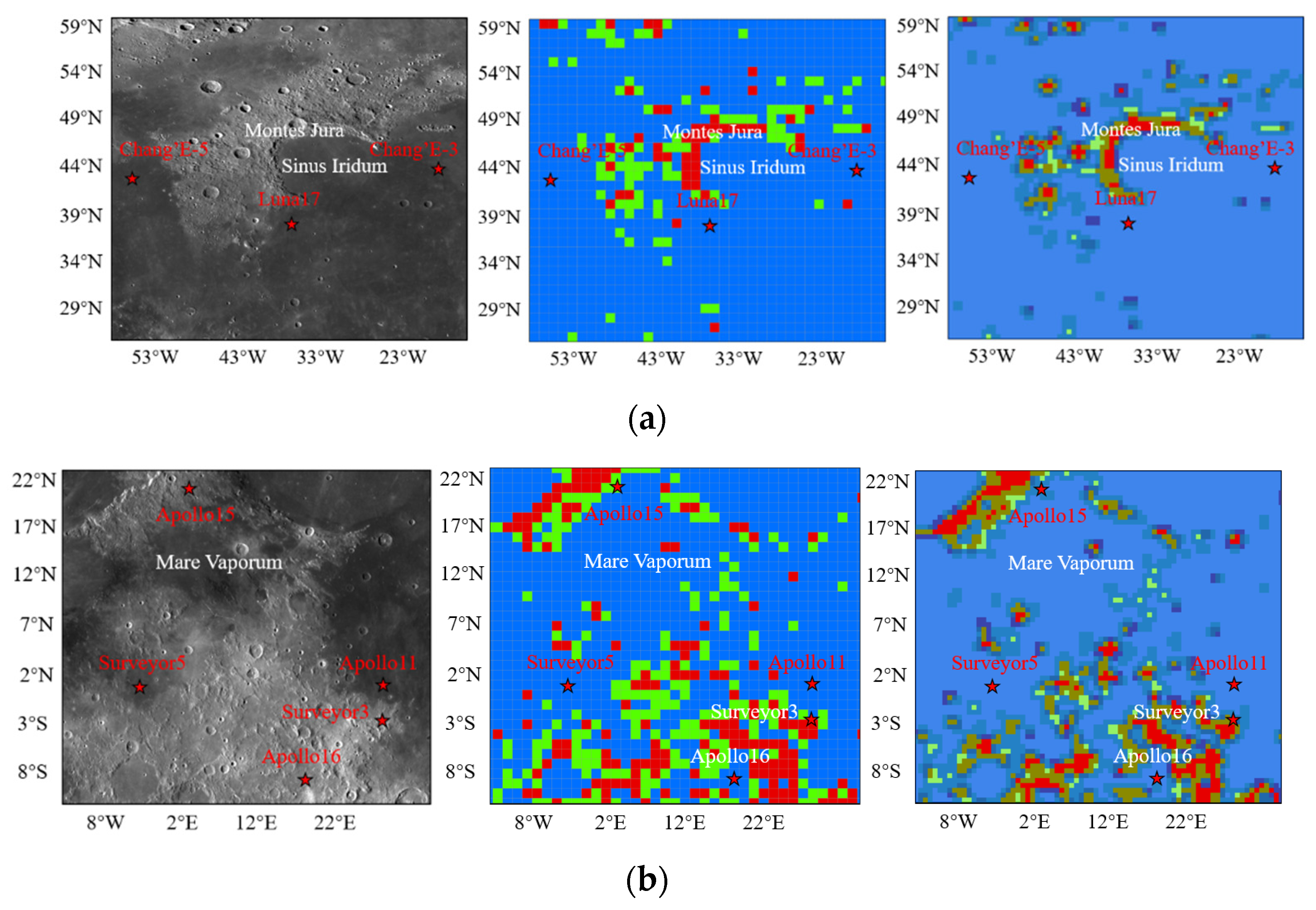
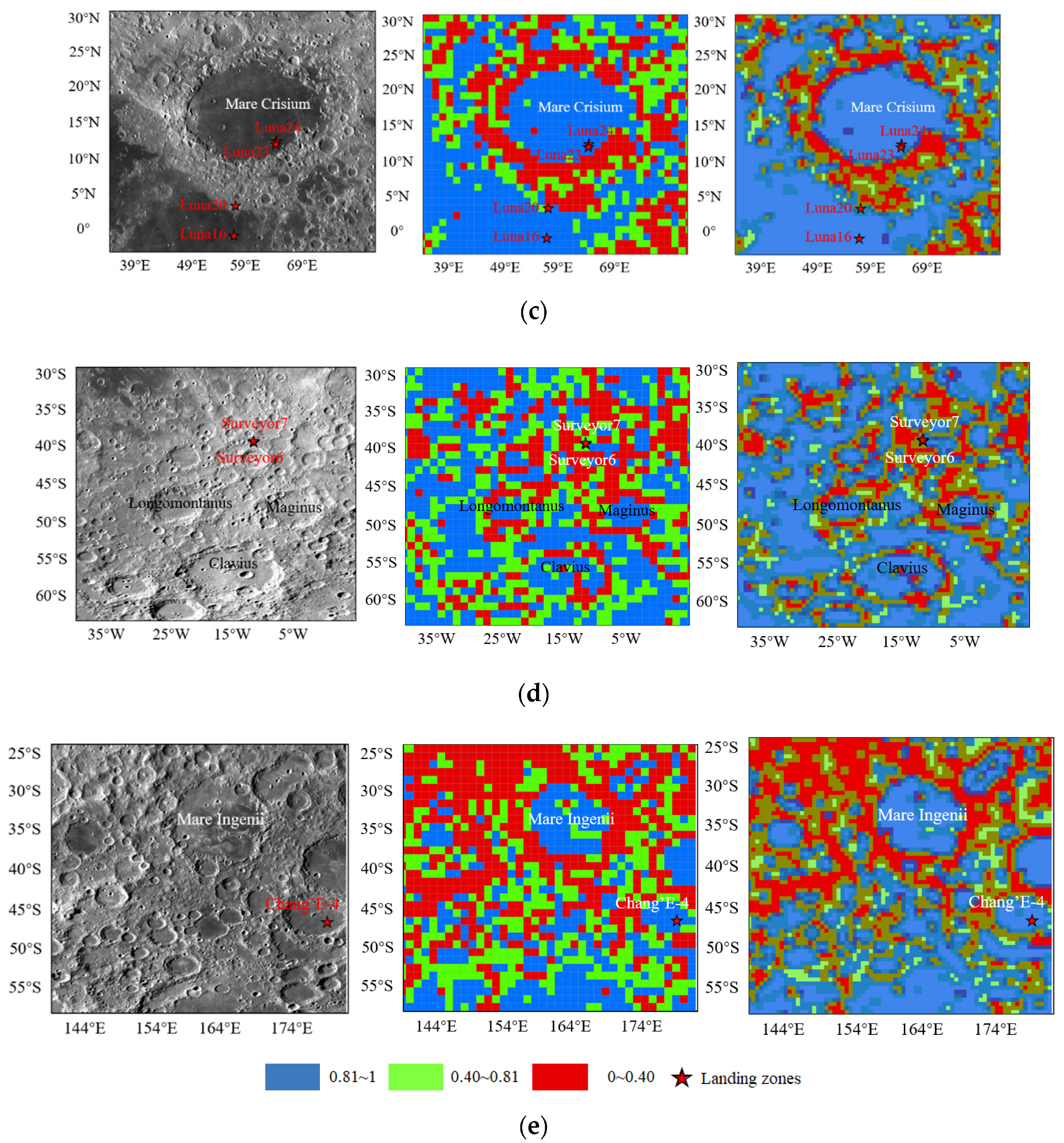
3.2. Comparison of Sliding Window and Grid Method
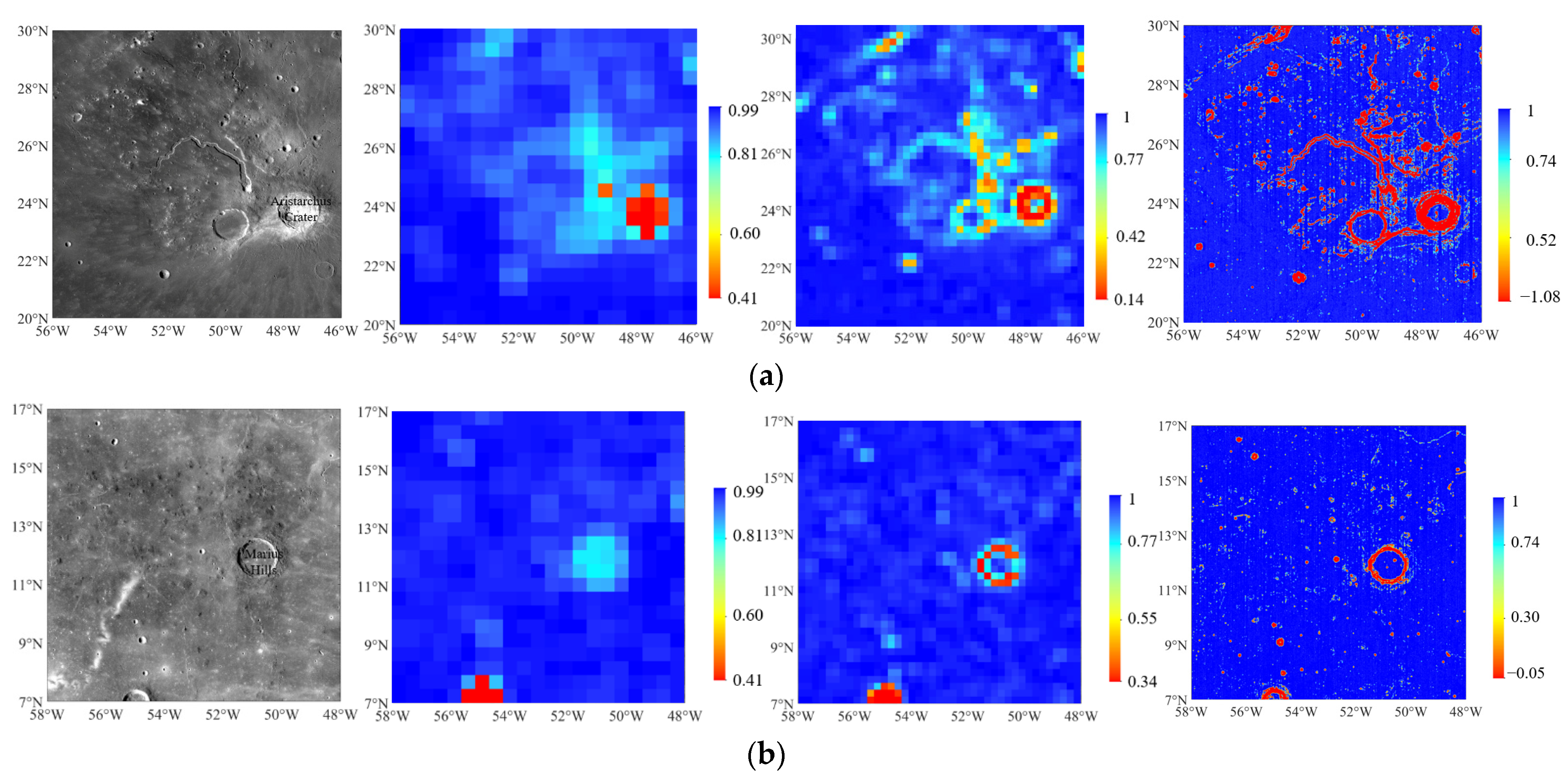
3.3. Evaluation of Lunar Candidate Landing Regions
4. Discussions
- The sliding window method causes all pixel points to participate in the operation more than once. The evaluation index in the range of the whole Moon needs 30 h to complete the calculation with a window size of 1° × 1° and a step size of 0.5°, which takes more than three days when each window is cut and presented. For the 10° × 10° candidate landing zones, the required computation time for all window sizes is about 150 s, which is still not sufficient even for evaluating the safety of the probe’s lunar surface landing site slope during descent. The required computation time is relatively long, and optimized calculation methods such as distributed computing and high-performance computing may need to be used to increase the computation speed.
- This study only confirms the effectiveness of this method; hence, it only analyzes slopes with an engineering boundary condition. The amount of rock [86,87], the roughness of the lunar surface, the lighting conditions, the polar terrain for water ice [88], and the communication conditions are also central to the technical considerations. The integration of these data, the quantification of land suitability, and the comprehensive index weighting of data from multiple sources can be further researched.
5. Conclusions
Author Contributions
Funding
Data Availability Statement
Acknowledgments
Conflicts of Interest
References
- Li, C.; Wang, C.; Wei, Y.; Lin, Y. China’s present and future lunar exploration program. Science 2019, 365, 238–239. [Google Scholar] [CrossRef]
- De Rosa, D.; Bussey, B.; Cahill, J.T.; Lutz, T.; Crawford, I.A.; Hackwill, T.; van Gasselt, S.; Neukum, G.; Witte, L.; McGovern, A.; et al. Characterisation of potential landing sites for the European Space Agency’s Lunar Lander project. Planet. Space Sci. 2012, 74, 224–246. [Google Scholar] [CrossRef] [Green Version]
- Djachkova, M.V.; Litvak, M.L.; Mitrofanov, I.G.; Sanin, A.B. Selection of Luna-25 landing sites in the South Polar Region of the Moon. Sol. Syst. Res. 2017, 51, 185–195. [Google Scholar] [CrossRef]
- ESA. ESA Strategy for Science at the Moon. Available online: https://exploration.esa.int/web/moon/-/61371-esastrategy-for-science-at-the-moon (accessed on 8 October 2019).
- Hashimoto, T.; Hoshino, T.; Tanaka, S.; Otsuki, M.; Otake, H.; Morimoto, H. Japanese moon lander SELENE-2—Present status in 2009. Acta Astronaut. 2011, 68, 1386–1391. [Google Scholar] [CrossRef]
- NASA. NASA Seeks US Partners to Develop Reusable Systems to Land Astronauts on Moon. Available online: https://www.nasa.gov/feature/nasa-seeks-us-partners-to-develop-reusable-systems-to-land-astronautson-moon (accessed on 8 October 2019).
- Singh, A.; Srinivasan, T. Potential Landing Sites for Chandrayaan-2 Lander in Southern Hemisphere of Moon. In Proceedings of the Lunar and Planetary Science Conference, The Woodlands, TX, USA, 18–22 March 2019. [Google Scholar]
- Ouyang, Z.Y. An Introduction to Lunar Science; China Astronautic Publishing House: Beijing, China, 2005. [Google Scholar]
- NRC. Scientific Context for the Exploration of the Moon; National Academies Press: Washington, DC, USA, 2007. [Google Scholar]
- LEAG. Advancing Science of the Moon Specific Action Team Report. In Proceedings of the Advancing Science of the Moon: Report of the Specific Action Team, Houston, TX, USA, 7–8 August 2017. [Google Scholar]
- Boazman, S.; Kereszturi, A.; Heather, D.; Sefton-Nash, E.; Orgel, C.; Tomka, R.; Houdou, B.; Lefort, X. Analysis of the Lunar South Polar Region for PROSPECT, NASA/CLPS. In Proceedings of the European Planetary Science Congress, Granada, Spain, 18–23 September 2022; pp. EPSC2022–EPSC2530. [Google Scholar]
- Jawin, E.R.; Valencia, S.N.; Watkins, R.N.; Crowell, J.M.; Neal, C.R.; Schmidt, G. Lunar Science for Landed Missions Workshop Findings Report. Earth Space Sci. 2019, 6, 2–40. [Google Scholar] [CrossRef] [Green Version]
- Liu, N.; Jin, Y.Q. Selection of a Landing Site in the Permanently Shadowed Portion of Lunar Polar Regions Using DEM and Mini-RF Data. IEEE Geosci. Remote Sens. Lett. 2022, 19, 2–40. [Google Scholar] [CrossRef]
- Slyuta, E. CHAPTER 3–The Luna program. In Sample Return Missions; Longobardo, A., Ed.; Elsevier: Amsterdam, The Netherlands, 2021; pp. 37–78. [Google Scholar]
- Newell, H.E. Surveyor III: A Preliminary Report; National Aeronautics and Space Administration: Washington, DC, USA, 1967. [Google Scholar]
- Center, M.S. Apollo 12: Preliminary Science Report; NASA Manned Spacecraft Center: Washington, DC, USA, 1970. [Google Scholar]
- Quaide, W.L.; Oberbeck, V.R. Geology of the Apollo landing sites. Earth-Sci. Rev. 1969, 5, 255–278. [Google Scholar] [CrossRef]
- Li, C.; Liu, J.; Zuo, W.; Su, Y.; Ouyang, Z.Y. Progress of China’s Lunar Exploration (2011–2020). Chin. J. Space Sci. 2021, 41, 68–75. [Google Scholar] [CrossRef]
- Zhang, H.; Guan, Y.; Huang, X.; Li, J.; Zhao, Y.; Yu, P.; Zhang, X.; Yang, W.; Liang, J.; Wang, D. Guidance navigation and control for Chang’E-3 powered descent. Sci. Sin. Technol. 2014, 339, 668–671. [Google Scholar] [CrossRef]
- Wu, W.; Li, C.; Zuo, W.; Zhang, H.; Liu, J.; Wen, W.; Su, Y.; Ren, X.; Yan, J.; Yu, D.; et al. Lunar farside to be explored by Chang’E-4. Nat. Geosci. 2019, 12, 222–223. [Google Scholar] [CrossRef]
- Zezhou, S.; TingXin, Z.; He, Z.-H.; Yang, J.; Honghua, Z.; Jianxin, C.; Xueying, W.; ZhenRong, S. The technical design and achievements of Chang’E-3 probe. Sci. Sin. Technol. 2014, 44, 331–343. [Google Scholar] [CrossRef] [Green Version]
- Li, C.; Liu, J.; Ren, X.; Zuo, W.; Tan, X.; Wen, W.; Li, H.; Mu, L.; Su, Y.; Zhang, H.; et al. The Chang’E 3 Mission Overview. Space Sci. Rev. 2015, 190, 85–101. [Google Scholar] [CrossRef]
- Li, C.-L.; Mu, L.-L.; Zou, X.-D.; Liu, J.-J.; Ren, X.; Zeng, X.-G.; Yang, Y.-M.; Zhang, Z.-B.; Liu, Y.-X.; Zuo, W.; et al. Analysis of the geomorphology surrounding the Chang’E-3 landing site. Res. Astron. Astrophys. 2014, 14, 1514–1529. [Google Scholar] [CrossRef]
- Jia, Y.; Zou, Y.; Ping, J.; Xue, C.; Yan, J.; Ning, Y. The scientific objectives and payloads of Chang’E−4 mission. Planet. Space Sci. 2018, 162, 207–215. [Google Scholar] [CrossRef]
- Liu, J.; Ren, X.; Yan, W.; Li, C.; Zhang, H.; Jia, Y.; Zeng, X.; Chen, W.; Gao, X.; Liu, D.; et al. Descent trajectory reconstruction and landing site positioning of Chang’E-4 on the lunar farside. Nat. Commun. 2019, 10, 4229. [Google Scholar] [CrossRef] [Green Version]
- Qian, Y.Q.; Xiao, L.; Zhao, S.Y.; Zhao, J.N.; Huang, J.; Flahaut, J.; Martinot, M.; Head, J.W.; Hiesinger, H.; Wang, G.X. Geology and Scientific Significance of the Rümker Region in Northern Oceanus Procellarum: China’s Chang’E-5 Landing Region. J. Geophys. Res. Planets 2018, 123, 1407–1430. [Google Scholar] [CrossRef] [Green Version]
- Nesvorný, D.; Roig, F.V.; Vokrouhlický, D.; Bottke, W.F.; Marchi, S.; Morbidelli, A.; Deienno, R. Early bombardment of the moon: Connecting the lunar crater record to the terrestrial planet formation. Icarus 2023, 399, 115545. [Google Scholar] [CrossRef]
- Kereszturi, A.; Steinmann, V. Terra-mare comparison of small young craters on the Moon. Icarus 2019, 322, 54–68. [Google Scholar] [CrossRef]
- Liu, J.; Zeng, X.; Li, C.; Ren, X.; Yan, W.; Tan, X.; Zhang, X.; Chen, W.; Zuo, W.; Liu, Y.; et al. Landing Site Selection and Overview of China’s Lunar Landing Missions. Space Sci. Rev. 2020, 217, 6. [Google Scholar] [CrossRef]
- Flahaut, J.; Blanchette-Guertin, J.F.; Jilly, C.; Sharma, P.; Souchon, A.; van Westrenen, W.; Kring, D.A. Identification and characterization of science-rich landing sites for lunar lander missions using integrated remote sensing observations. Adv. Space Res. 2012, 50, 1647–1665. [Google Scholar] [CrossRef]
- Lemelin, M.; Blair, D.M.; Roberts, C.E.; Runyon, K.D.; Nowka, D.; Kring, D.A. High-priority lunar landing sites for in situ and sample return studies of polar volatiles. Planet. Space Sci. 2014, 101, 149–161. [Google Scholar] [CrossRef]
- Liang, H.; Ren, Q.; Feng, Y.; Zhang, J.; Liu, S.; Chen, S. Real-time dynamic addressing for spacecraft soft landing in the lunar surface. In Proceedings of the 2015 IEEE International Conference on Information and Automation, Lijiang, China, 8–10 August 2015; pp. 987–992. [Google Scholar]
- Flahaut, J.; Carpenter, J.; Williams, J.P.; Anand, M.; Crawford, I.A.; van Westrenen, W.; Füri, E.; Xiao, L.; Zhao, S. Regions of interest (ROI) for future exploration missions to the lunar South Pole. Planet. Space Sci. 2020, 180, 104750. [Google Scholar] [CrossRef]
- Xingguo, Z.; Lingli, M. Lunar Spatial Environmental Indicators Dynamically Modeling Based Exploration Area Selection. Geomat. Inf. Sci. Wuhan Univ. 2017, 42, 91–96. [Google Scholar] [CrossRef]
- Zhiguo, M.; Cui, L.; Jinsong, P.; Qian, H.; Zhanchuan, C.; Gusev, A. Analysis About Landing Site Selection and Prospective Scientific Objectives of the Von Kármán Crater in Moon Farside. J. Deep Space Explor. 2018, 5, 3–11. [Google Scholar]
- Xiao, L.; Qiao, L.; Xiao, Z.; Huang, Q.; He, Q.; Zhao, J.; Xue, Z.; Huang, J. Major scientific objectives and candidate landing sites suggested for future lunar explorations. Sci. Sin. Phys. Mech. Astron. 2016, 46, 029602. [Google Scholar] [CrossRef] [Green Version]
- Kereszturi, A. Polar Ice on the Moon. In Encyclopedia of Lunar Science; Cudnik, B., Ed.; Springer International Publishing: Cham, Switzerland, 2020; pp. 1–9. [Google Scholar]
- Amitabh, S.; Srinivasan, T.P.; Suresh, K. Potential Landing Sites for Chandrayaan-2 Lander in Southern Hemisphere of Moon. In Proceedings of the 49th Annual Lunar and Planetary Science Conference, The Woodlands, TX, USA, 19–23 March 2018; p. 1975. [Google Scholar]
- Deitrick, S.R.; Russell, A.T.; Loza, S.B. Landing Site Analysis for a Lunar Polar Water Ice Ground Truth Mission. In Lunar Surface Science Workshop; Universities Space Research Association: Washington, DC, USA, 2020; p. 5120. [Google Scholar]
- Ehlmann, B. Lunar Trailblazer: A Pioneering Smallsat for Lunar Water and Lunar Geology. In Proceedings of the 44th COSPAR Scientific Assembly, Athens, Greece, 16-–24 July 2022; p. 301. [Google Scholar]
- Wei, G.; Li, X.; Zhang, W.; Tian, Y.; Jiang, S.; Wang, C.; Ma, J. Illumination conditions near the Moon’s south pole: Implication for a concept design of China’s Chang’E-7 lunar polar exploration. Acta Astronaut. 2023, 208, 74–81. [Google Scholar] [CrossRef]
- Golombek, M.; Parker, T.; Kass, D.; Crisp, J.; Squyres, S.; Carr, M.; Adler, M.; Zurek, R.; Haldermann, A. Selection of the Final Four Landing Sites for the Mars Exploration Rovers. In Proceedings of the Lunar and Planetary Science Conference, Houston, TX, USA, 17–21 March 2003; p. 1754. [Google Scholar]
- Chen, S.; Li, Y.; Zhang, T.; Zhu, X.; Sun, S.; Gao, X. Lunar features detection for energy discovery via deep learning. Appl. Energy 2021, 296, 117085. [Google Scholar] [CrossRef]
- Jia, Y.; Liu, L.; Wang, X.; Guo, N.; Wan, G. Selection of Lunar South Pole Landing Site Based on Constructing and Analyzing Fuzzy Cognitive Maps. Remote Sens. 2022, 14, 4863. [Google Scholar] [CrossRef]
- Darlan, D.; Ajani, O.S.; Mallipeddi, R. Lunar Landing Site Selection using Machine Learning. In Proceedings of the 2023 International Conference on Machine Intelligence for GeoAnalytics and Remote Sensing (MIGARS), Hyderabad, India, 27–29 January 2023; pp. 1–4. [Google Scholar]
- Cao, Y.; Wang, Y.; Liu, J.; Zeng, X.; Wang, J. Selection of Whole-Moon Landing Zones Based on Weights of Evidence and Fractals. Remote Sens. 2022, 14, 4623. [Google Scholar] [CrossRef]
- Song, L.; Wang, J.; Zhang, Y.; Zhao, F.; Zhu, S.; Jiang, L.; Du, Q.; Zhao, X.; Li, Y. Sliding Window Detection and Analysis Method of Night-Time Light Remote Sensing Time Series—A Case Study of the Torch Festival in Yunnan Province, China. Remote Sens. 2022, 14, 5267. [Google Scholar] [CrossRef]
- Yin, Q.; Chen, Z.; Zheng, X.; Xu, Y.; Liu, T. Sliding Windows Method Based on Terrain Self-Similarity for Higher DEM Resolution in Flood Simulating Modeling. Remote Sens. 2021, 13, 3604. [Google Scholar] [CrossRef]
- Rajashekara, H.M.; Nagajothi, K.; Sanda, A.V.; Sagar, B.S.D. Categorization of hierarchically partitioned waterbody-spread via Moran’s index. In Proceedings of the 2017 IEEE International Geoscience and Remote Sensing Symposium (IGARSS), Fort Worth, TX, USA, 23–28 July 2017; pp. 5567–5570. [Google Scholar]
- Chin, G.; Brylow, S.; Foote, M.; Garvin, J.; Kasper, J.; Keller, J.; Litvak, M.; Mitrofanov, I.; Paige, D.; Raney, K.; et al. Lunar Reconnaissance Orbiter Overview: The Instrument Suite and Mission. Space Sci. Rev. 2007, 129, 391–419. [Google Scholar] [CrossRef]
- Vondrak, R.; Keller, J.; Chin, G.; Garvin, J. Lunar Reconnaissance Orbiter (LRO): Observations for Lunar Exploration and Science. Space Sci. Rev. 2010, 150, 7–22. [Google Scholar] [CrossRef]
- Smith, D.E.; Zuber, M.T.; Jackson, G.B.; Cavanaugh, J.F.; Neumann, G.A.; Riris, H.; Sun, X.; Zellar, R.S.; Coltharp, C.; Connelly, J.; et al. The Lunar Orbiter Laser Altimeter Investigation on the Lunar Reconnaissance Orbiter Mission. Space Sci. Rev. 2010, 150, 209–241. [Google Scholar] [CrossRef]
- Mazarico, E.; Rowlands, D.D.; Neumann, G.A.; Smith, D.E.; Torrence, M.H.; Lemoine, F.G.; Zuber, M.T. Orbit determination of the Lunar Reconnaissance Orbiter. J. Geod. 2012, 86, 193–207. [Google Scholar] [CrossRef]
- Burrough, P.A.; McDonnell, R. Principles of Geographical Information Systems; Oxford Univ. Press: Oxford, UK, 1998. [Google Scholar]
- Smith, D.E.; Zuber, M.T.; Neumann, G.A.; Mazarico, E.; Lemoine, F.G.; Head Iii, J.W.; Lucey, P.G.; Aharonson, O.; Robinson, M.S.; Sun, X.; et al. Summary of the results from the lunar orbiter laser altimeter after seven years in lunar orbit. Icarus 2017, 283, 70–91. [Google Scholar] [CrossRef] [Green Version]
- Barker, M.K.; Mazarico, E.; Neumann, G.A.; Zuber, M.T.; Haruyama, J.; Smith, D.E. A new lunar digital elevation model from the Lunar Orbiter Laser Altimeter and SELENE Terrain Camera. Icarus 2016, 273, 346–355. [Google Scholar] [CrossRef] [Green Version]
- Altunkaynak, B.; Gamgam, H. Bootstrap confidence intervals for the coefficient of quartile variation. Commun. Stat.-Simul. Comput. 2019, 48, 2138–2146. [Google Scholar] [CrossRef]
- Moran, P.A.P. The Interpretation of Statistical Maps. J. R. Stat. Soc. Ser. B (Methodol.) 1948, 10, 243–251. [Google Scholar] [CrossRef]
- Kaliraj, S.; Chandrasekar, N.; Magesh, N.S. Identification of potential groundwater recharge zones in Vaigai upper basin, Tamil Nadu, using GIS-based analytical hierarchical process (AHP) technique. Arab. J. Geosci. 2014, 7, 1385–1401. [Google Scholar] [CrossRef]
- Rahaman, S.A.; Ajeez, S.A.; Aruchamy, S.; Jegankumar, R. Prioritization of Sub Watershed Based on Morphometric Characteristics Using Fuzzy Analytical Hierarchy Process and Geographical Information System—A Study of Kallar Watershed, Tamil Nadu. Aquat. Procedia 2015, 4, 1322–1330. [Google Scholar] [CrossRef]
- Wang, X.; Mao, L.; Yue, Y.; Zhao, J. Manned lunar landing mission scale analysis and flight scheme selection based on mission architecture matrix. Acta Astronaut. 2018, 152, 385–395. [Google Scholar] [CrossRef]
- Saaty, R.W. The analytic hierarchy process—What it is and how it is used. Math. Model. 1987, 9, 161–176. [Google Scholar] [CrossRef] [Green Version]
- Saaty, T.L. Group Decision Making and the AHP. In The Analytic Hierarchy Process: Applications and Studies; Golden, B.L., Wasil, E.A., Harker, P.T., Eds.; Springer: Berlin/Heidelberg, Germany, 1989; pp. 59–67. [Google Scholar]
- Brunelli, M. Introduction to the Analytic Hierarchy Process; Springer: Cham, Switzerland, 2015. [Google Scholar]
- Saaty, T.L. How to make a decision: The analytic hierarchy process. Eur. J. Oper. Res. 1990, 48, 9–26. [Google Scholar] [CrossRef]
- Saaty, T.L. Decision making for leaders. IEEE Trans. Syst. Man Cybern. 1985, SMC-15, 450–452. [Google Scholar] [CrossRef]
- Jain, A.K.; Dubes, R.C. Algorithms for Clustering Data; Prentice-Hall: Englewood Cliffs, NJ, USA, 1988. [Google Scholar]
- MacQueen, J. Some methods for classification and analysis of multivariate observations. In Proceedings of the Berkeley Symposium on Mathematical Statistics and Probability, Statistical Laboratory of the University of California, Berkeley, CA, USA, 1 January 1967; pp. 281–297. [Google Scholar]
- Luo, M.; Yu-Fei, M.; Hong-Jiang, Z. A spatial constrained K-means approach to image segmentation. In Proceedings of the Fourth International Conference on Information, Communications and Signal Processing, 2003 and the Fourth Pacific Rim Conference on Multimedia. Proceedings of the 2003 Joint, Singapore, 15–18 December 2003; Volume 732, pp. 738–742. [Google Scholar]
- Sinaga, K.P.; Yang, M.S. Unsupervised K-Means Clustering Algorithm. IEEE Access 2020, 8, 80716–80727. [Google Scholar] [CrossRef]
- Maheshwary, P.; Srivastav, N. Retrieving Similar Image Using Color Moment Feature Detector and K-Means Clustering of Remote Sensing Images. In Proceedings of the 2008 International Conference on Computer and Electrical Engineering, Dhaka, Bangladesh, 20–22 December 2008; pp. 821–824. [Google Scholar]
- Tibshirani, R.; Walther, G.; Hastie, T. Estimating the number of clusters in a data set via the gap statistic. J. R. Stat. Soc. Ser. B (Stat. Methodol.) 2001, 63, 411–423. [Google Scholar] [CrossRef]
- Jin, X.; Han, J. K-Means Clustering. In Encyclopedia of Machine Learning; Sammut, C., Webb, G.I., Eds.; Springer: Boston, MA, USA, 2010; pp. 563–564. [Google Scholar]
- Basilevsky, A.T.; Abdrakhimov, A.M.; Head, J.W.; Pieters, C.M.; Wu, Y.; Xiao, L. Geologic characteristics of the Luna 17/Lunokhod 1 and Chang’E-3/Yutu landing sites, Northwest Mare Imbrium of the Moon. Planet. Space Sci. 2015, 117, 385–400. [Google Scholar] [CrossRef]
- Séjourné, A.; Costard, F.; Swirad, Z.M.; Łosiak, A.; Bouley, S.; Smith, I.; Balme, M.R.; Orgel, C.; Ramsdale, J.D.; Hauber, E.; et al. Grid Mapping the Northern Plains of Mars: Using Morphotype and Distribution of Ice-Related Landforms to Understand Multiple Ice-Rich Deposits in Utopia Planitia. J. Geophys. Res. Planets 2019, 124, 483–503. [Google Scholar] [CrossRef] [Green Version]
- Mustard, J.F.; Pieters, C.M.; Isaacson, P.J.; Head, J.W.; Besse, S.; Clark, R.N.; Klima, R.L.; Petro, N.E.; Staid, M.I.; Sunshine, J.M.; et al. Compositional diversity and geologic insights of the Aristarchus crater from Moon Mineralogy Mapper data. J. Geophys. Res. Planets 2011, 116, E00G12. [Google Scholar] [CrossRef] [Green Version]
- Ling, Z.; Zhang, J.; Wu, Z.; Sun, L.; Liu, J. The compositional distribution and rock types of the Aristarchus region on the Moon. Sci. Sin. Phys. Mech. Astron. 2013, 43, 1403–1410. [Google Scholar] [CrossRef]
- Lucey, P.G.; Hawke, B.R.; Pieters, C.M.; Head, J.W.; McCord, T.B. A compositional study of the Aristarchus Region of the Moon using near-infrared reflectance spectroscopy. J. Geophys. Res. Solid Earth 1986, 91, 344–354. [Google Scholar] [CrossRef] [Green Version]
- Huang, J.; Xiao, L.; He, X.; Qiao, L.; Zhao, J.; Li, H. Geological characteristics and model ages of Marius Hills on the Moon. J. Earth Sci. 2011, 22, 601–609. [Google Scholar] [CrossRef]
- Hargitai, H.; Kereszturi, A. Encyclopedia of Planetary Landforms; Springer: Berlin, Germany, 2015. [Google Scholar]
- Pieters, C.M.; Head, J.W.; Adams, J.B.; McCord, T.B.; Zisk, S.H.; Whitford-Stark, J.L. Late high-titanium basalts of the Western Maria: Geology of the Flamsteed REgion of Oceanus Procellarum. J. Geophys. Res. Solid Earth 1980, 85, 3913–3938. [Google Scholar] [CrossRef] [Green Version]
- Wieczorek, M.A.; Neumann, G.A.; Nimmo, F.; Kiefer, W.S.; Taylor, G.J.; Melosh, H.J.; Phillips, R.J.; Solomon, S.C.; Andrews-Hanna, J.C.; Asmar, S.W.; et al. The Crust of the Moon as Seen by GRAIL. Science 2013, 339, 671–675. [Google Scholar] [CrossRef]
- Pieters, C.; Moriarty, D.; Garrick-Bethell, I. Atypical Regolith Processes Hold the Key to Enigmatic Lunar Swirls. In Proceedings of the 45th Lunar Planet Science Conference, The Woodlands, TX, USA, 17–21 March 2014. [Google Scholar]
- Whitten, J.; Head, J.W.; Staid, M.; Pieters, C.M.; Mustard, J.; Clark, R.; Nettles, J.; Klima, R.L.; Taylor, L. Lunar mare deposits associated with the Orientale impact basin: New insights into mineralogy, history, mode of emplacement, and relation to Orientale Basin evolution from Moon Mineralogy Mapper (M3) data from Chandrayaan-1. J. Geophys. Res. Planets 2011, 116, E00G09. [Google Scholar] [CrossRef] [Green Version]
- Kring, D.A.; Durda, D.D. A global lunar landing site study to provide the scientific context for exploration of the Moon. In Proceedings of the LPI Contribution No. 1694. LPI-JSC Center for Lunar Science and Exploration, Houston, TX, USA; 2012. [Google Scholar]
- Jia, B.; Fa, W.; Xie, M.; Tai, Y.; Liu, X. Regolith Properties in the Chang’E-5 Landing Region of the Moon: Results From Multi-Source Remote Sensing Observations. J. Geophys. Res. Planets 2021, 126, e2021JE006934. [Google Scholar] [CrossRef]
- Zhang, L.; Xu, Y.; Bugiolacchi, R.; Hu, B.; Liu, C.; Lai, J.; Zeng, Z.; Huo, Z. Rock abundance and evolution of the shallow stratum on Chang’E-4 landing site unveiled by lunar penetrating radar data. Earth Planet. Sci. Lett. 2021, 564, 116912. [Google Scholar] [CrossRef]
- Kereszturi, A.; Boazman, S.J.; Heather, D.; Tomka, R.; Warren, T. Comparison of Landing Regions at the Southern Lunar Polar Terrain for Water Ice Access. In Proceedings of the Lunar Polar Volatiles Conference, Virtual, 2–4 November 2022; p. 5038. [Google Scholar]


| Strength of Significance | Explanation |
|---|---|
| 1 | Equal significance |
| 3 | Medium significance |
| 5 | Strong significance |
| 7 | Very strong significance |
| 9 | Maximum significance |
| 2, 4, 6, 8 | Interim number between two adjacent numbers |
| Factor | Mean Slope | Threshold Ratio (8) | Threshold Ratio (20) | Coefficient of Variation | Moran’s I | Normalized Principal Eigenvector |
|---|---|---|---|---|---|---|
| Mean slope | 1 | 1 | 5 | 3 | 7 | 36.32% |
| Threshold ratio (8) | 1 | 1 | 5 | 3 | 7 | 36.32% |
| Threshold ratio (20) | 1/5 | 1/5 | 1 | 1/3 | 3 | 7.67% |
| Coefficient of variation | 1/5 | 1/5 | 3 | 1 | 7 | 15.78% |
| Moran’s I | 1/7 | 1/7 | 1/3 | 1/5 | 1 | 3.91% |
| Total | 100.00% |
| n | 1 | 2 | 3 | 4 | 5 | 6 |
|---|---|---|---|---|---|---|
| RI | 0 | 0 | 0.58 | 0.90 | 1.12 | 1.24 |
| No. | Detector | Average | Threshold Ratio (8) * | Cv * | Moran’s I | Threshold Ratio (20) * | Overall Rating (1) * | Overall Rating (0.5) * |
|---|---|---|---|---|---|---|---|---|
| 1 | Luna9 | 2.82 | 0.88 | 0.37 | 0.97 | 0.98 | 0.90 | 0.82 |
| 1.66 | 0.95 | 0.23 | 0.96 | 0.99 | 0.94 | 0.77 | ||
| 4.99 | 0.77 | 0.54 | 0.97 | 0.98 | 0.83 | 0.86 | ||
| 2.72 | 0.91 | 0.31 | 0.95 | 0.99 | 0.92 | 0.81 | ||
| 2 | Luna13 | 0.46 | 0.99 | 0.05 | 0.82 | 1 | 0.98 | 0.97 |
| 0.42 | 0.99 | 0.04 | 0.82 | 1 | 0.98 | 0.97 | ||
| 0.55 | 0.99 | 0.08 | 0.93 | 1 | 0.98 | 0.98 | ||
| 0.64 | 0.99 | 0.08 | 0.93 | 1 | 0.98 | 0.98 | ||
| 3 | Luna16 | 0.86 | 1 | 0.03 | 0.78 | 1 | 0.99 | 0.96 |
| 0.88 | 1 | 0.06 | 0.86 | 1 | 0.99 | 0.96 | ||
| 0.97 | 1 | 0.03 | 0.84 | 1 | 0.99 | 0.97 | ||
| 1 | 1 | 0.04 | 0.83 | 1 | 0.99 | 0.97 | ||
| 4 | Luna17 | 0.57 | 0.99 | 0.08 | 0.89 | 1 | 0.98 | 0.98 |
| 0.66 | 0.99 | 0.10 | 0.91 | 1 | 0.98 | 0.98 | ||
| 0.53 | 1 | 0.05 | 0.82 | 1 | 0.99 | 0.98 | ||
| 0.09 | 0.99 | 0.09 | 0.89 | 1 | 0.98 | 0.98 | ||
| 5 | Luna20 | 7.72 | 0.61 | 0.79 | 0.95 | 0.98 | 0.73 | 0.24 |
| 7.06 | 0.68 | 0.68 | 0.951 | 0.98 | 0.77 | 0.32 | ||
| 8.19 | 0.57 | 0.87 | 0.95 | 0.97 | 0.34 | 0.76 | ||
| 7.50 | 0.65 | 0.73 | 0.96 | 0.95 | 0.75 | 0.75 | ||
| 6 | Luna21 | 2.33 | 0.95 | 0.23 | 0.95 | 1 | 0.94 | 0.98 |
| 2.77 | 0.88 | 0.36 | 0.98 | 0.98 | 0.90 | 0.89 | ||
| 4.28 | 0.87 | 0.39 | 0.95 | 0.99 | 0.89 | 0.98 | ||
| 5.97 | 0.71 | 0.64 | 0.96 | 0.98 | 0.79 | 0.83 | ||
| 7 | Luna23 | 2.38 | 0.94 | 0.25 | 0.98 | 0.97 | 0.94 | 0.97 |
| 1.45 | 0.99 | 0.10 | 0.89 | 1 | 0.98 | 0.98 | ||
| 1.32 | 0.99 | 0.11 | 0.89 | 1 | 0.97 | 0.96 | ||
| 1.55 | 0.99 | 0.11 | 0.89 | 1 | 0.97 | 0.98 | ||
| 8 | Luna24 | 1.32 | 0.99 | 0.11 | 0.89 | 1 | 0.97 | 0.98 |
| 1.55 | 0.99 | 0.11 | 0.89 | 1 | 0.97 | 0.98 | ||
| 1.08 | 0.99 | 0.08 | 0.88 | 1 | 0.98 | 0.98 | ||
| 1.40 | 0.99 | 0.09 | 0.89 | 1 | 0.98 | 0.97 | ||
| 9 | Surveyor1 | 1.39 | 0.96 | 0.20 | 0.95 | 1 | 0.95 | 0.98 |
| 1.56 | 0.96 | 0.19 | 0.94 | 1 | 0.95 | 0.98 | ||
| 0.62 | 1 | 0.05 | 0.82 | 1 | 0.99 | 0.98 | ||
| 1.16 | 0.99 | 0.11 | 0.92 | 1 | 0.98 | 0.98 | ||
| 10 | Surveyor3 | 5.42 | 0.79 | 0.52 | 0.93 | 0.99 | 0.84 | 0.76 |
| 5.9 | 0.75 | 0.58 | 0.93 | 0.99 | 0.81 | 0.74 | ||
| 7.10 | 0.65 | 0.74 | 0.95 | 0.98 | 0.75 | 0.80 | ||
| 5.80 | 0.75 | 0.57 | 0.94 | 0.99 | 0.82 | 0.82 | ||
| 11 | Surveyor5 | 0.95 | 0.99 | 0.08 | 0.85 | 1 | 0.98 | 0.98 |
| 0.88 | 1 | 0.07 | 0.86 | 1 | 0.98 | 0.97 | ||
| 0.96 | 0.99 | 0.09 | 0.84 | 1 | 0.98 | 0.99 | ||
| 0.80 | 0.99 | 0.07 | 0.86 | 1 | 0.98 | 0.98 | ||
| 12 | Surveyor6 | 0.95 | 0.99 | 0.08 | 0.85 | 1 | 0.98 | 0.88 |
| 0.88 | 1 | 0.07 | 0.86 | 1 | 0.98 | 0.82 | ||
| 0.96 | 0.99 | 0.09 | 0.84 | 1 | 0.98 | 0.93 | ||
| 0.80 | 0.99 | 0.07 | 0.86 | 1 | 0.98 | 0.82 | ||
| 13 | Surveyor7 | 5.70 | 0.78 | 0.53 | 0.92 | 0.99 | 0.83 | 0.83 |
| 5.26 | 0.82 | 0.47 | 0.91 | 1.0 | 0.86 | 0.88 | ||
| 5.82 | 0.77 | 0.55 | 0.93 | 1 | 0.83 | 0.87 | ||
| 7.01 | 0.65 | 0.73 | 0.96 | 0.98 | 0.75 | 0.93 | ||
| 14 | Apollo11 | 1.47 | 0.98 | 0.15 | 0.93 | 1 | 0.97 | 0.96 |
| 1.22 | 0.98 | 0.13 | 0.92 | 1 | 0.97 | 0.96 | ||
| 1.43 | 0.98 | 0.14 | 0.92 | 1 | 0.97 | 0.97 | ||
| 1.17 | 0.99 | 0.10 | 0.89 | 1 | 0.98 | 0.98 | ||
| 15 | Apollo12 | 0.76 | 0.99 | 0.08 | 0.89 | 1 | 0.98 | 0.97 |
| 0.75 | 0.99 | 0.09 | 0.89 | 1 | 0.98 | 0.97 | ||
| 0.85 | 0.99 | 0.10 | 0.89 | 1 | 0.98 | 0.97 | ||
| 0.78 | 0.99 | 0.09 | 0.88 | 1 | 0.98 | 0.96 | ||
| 16 | Apollo14 | 3.30 | 0.95 | 0.23 | 0.87 | 1 | 0.94 | 0.95 |
| 3.28 | 0.95 | 0.23 | 0.87 | 1 | 0.94 | 0.94 | ||
| 3.38 | 0.95 | 0.23 | 0.87 | 1 | 0.94 | 0.95 | ||
| 3.94 | 0.90 | 0.34 | 0.93 | 1 | 0.91 | 0.95 | ||
| 17 | Apollo15 | 6.15 | 0.73 | 0.60 | 0.92 | 1 | 0.80 | 0.82 |
| 5.64 | 0.77 | 0.55 | 0.94 | 1 | 0.83 | 0.79 | ||
| 6.2 | 0.73 | 0.60 | 0.95 | 0.99 | 0.80 | 0.84 | ||
| 5.99 | 0.74 | 0.59 | 0.95 | 0.99 | 0.81 | 0.85 | ||
| 18 | Apollo16 | 4.25 | 0.86 | 0.41 | 0.91 | 1 | 0.88 | 0.87 |
| 5.24 | 0.82 | 0.48 | 0.92 | 0.99 | 0.85 | 0.87 | ||
| 4.44 | 0.82 | 0.46 | 0.93 | 0.99 | 0.86 | 0.86 | ||
| 5.34 | 0.80 | 0.50 | 0.92 | 1 | 0.85 | 0.82 | ||
| 19 | Apollo17 | 9.63 | 0.53 | 0.94 | 0.98 | 0.84 | 0.30 | 0.31 |
| 11.08 | 0.45 | 1.11 | 0.98 | 0.80 | 0.25 | 0.74 | ||
| 8.46 | 0.58 | 0.85 | 0.98 | 0.89 | 0.34 | 0.25 | ||
| 9.32 | 0.50 | 1.01 | 0.97 | 0.91 | 0.29 | 0.33 | ||
| 20 | CE-3 | 0.83 | 0.99 | 0.11 | 0.94 | 1 | 0.98 | 0.98 |
| 0.61 | 1 | 0.05 | 0.81 | 1 | 0.98 | 0.98 | ||
| 0.90 | 0.98 | 0.12 | 0.93 | 1 | 0.97 | 0.98 | ||
| 0.78 | 1 | 0.07 | 0.83 | 1 | 0.98 | 0.98 | ||
| 21 | CE-4 | 1.25 | 0.99 | 0.07 | 0.85 | 1 | 0.98 | 0.99 |
| 1.01 | 0.99 | 0.07 | 0.84 | 1 | 0.98 | 0.99 | ||
| 0.95 | 1 | 0.06 | 0.83 | 1 | 0.98 | 0.98 | ||
| 0.92 | 1 | 0.07 | 0.83 | 1 | 0.98 | 0.98 | ||
| 22 | CE-5 | 0.95 | 0.97 | 0.17 | 0.97 | 1 | 0.96 | 0.98 |
| 0.52 | 1 | 0.04 | 0.80 | 1 | 0.99 | 0.98 | ||
| 0.57 | 1 | 0.06 | 0.83 | 1 | 0.98 | 0.99 | ||
| 0.67 | 1 | 0.05 | 0.85 | 1 | 0.99 | 0.99 |
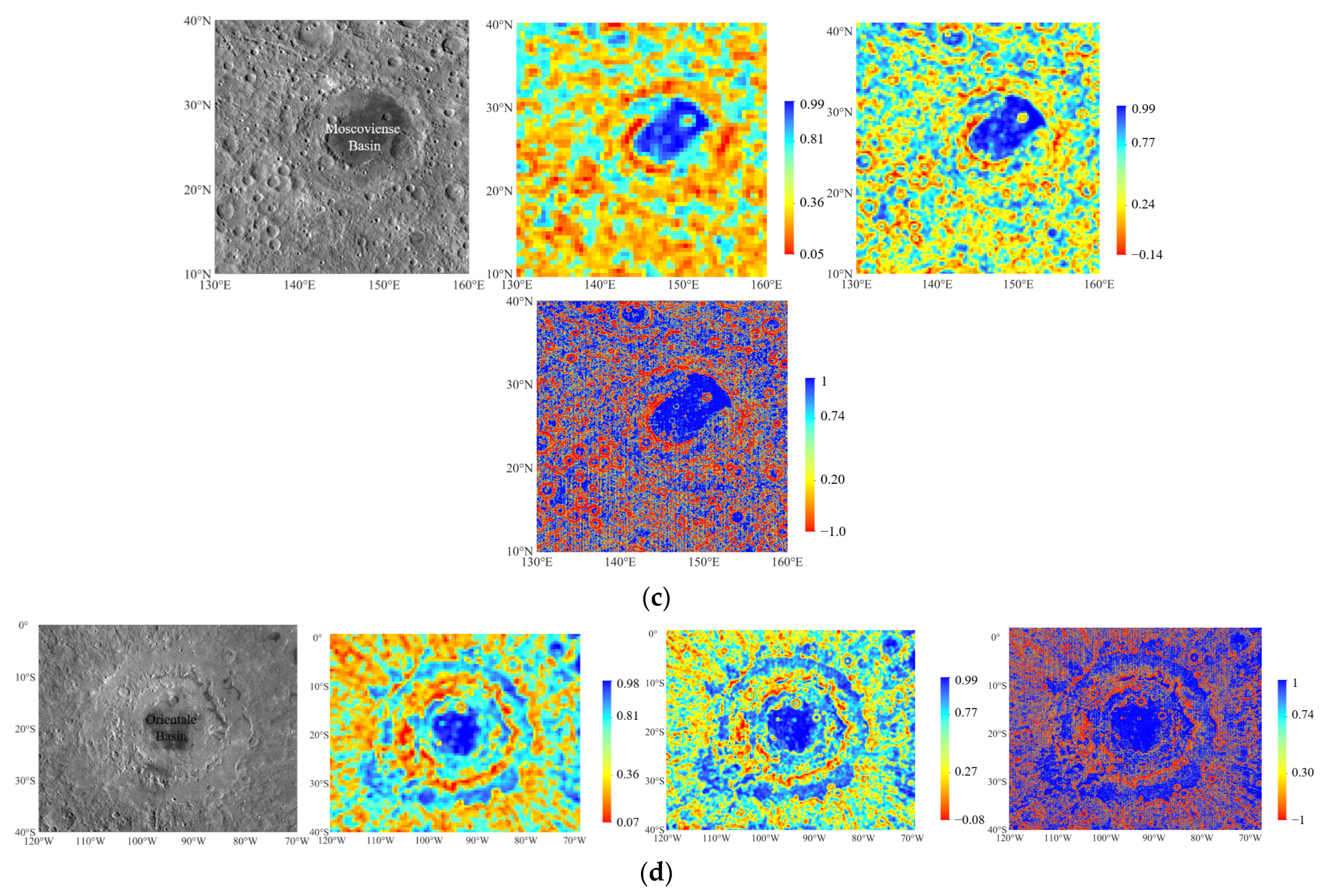
| No. | Candidate Landing Site | Window Size | Number of Suitable Windows | Total Number of Windows | Area of Candidate Landing Zones (km2) | Percentage of Suitable Landing Area |
|---|---|---|---|---|---|---|
| 1 | Aristarchus Crater | 1° × 1° | 407 | 441 | 100 | 0.92 |
| 0.5° × 0.5° | 1822 | 1935 | 0.94 | |||
| 0.03125° × 0.03125° | 369,306 | 408,321 | 0.90 | |||
| 2 | Marius Hills | 1° × 1° | 437 | 441 | 100 | 0.99 |
| 0.5° × 0.5° | 1653 | 1681 | 0.98 | |||
| 0.03125° × 0.03125° | 396,861 | 408,321 | 0.97 | |||
| 3 | Moscoviense Basin | 1° × 1° | 605 | 3660 | 900 | 0.17 |
| 0.5° × 0.5° | 3899 | 15,125 | 0.26 | |||
| 0.03125° × 0.03125° | 1,806,687 | 3,682,561 | 0.49 | |||
| 4 | Orientale Basin | 1° × 1° | 1713 | 8080 | 2000 | 0.21 |
| 0.5° × 0.5° | 12190 | 33,089 | 0.37 | |||
| 0.03125° × 0.03125° | 4,518,441 | 8,186,241 | 0.55 |
Disclaimer/Publisher’s Note: The statements, opinions and data contained in all publications are solely those of the individual author(s) and contributor(s) and not of MDPI and/or the editor(s). MDPI and/or the editor(s) disclaim responsibility for any injury to people or property resulting from any ideas, methods, instructions or products referred to in the content. |
© 2023 by the authors. Licensee MDPI, Basel, Switzerland. This article is an open access article distributed under the terms and conditions of the Creative Commons Attribution (CC BY) license (https://creativecommons.org/licenses/by/4.0/).
Share and Cite
Liu, H.; Wang, Y.; Wen, S.; Liu, J.; Wang, J.; Cao, Y.; Meng, Z.; Zhang, Y. A New Blind Selection Approach for Lunar Landing Zones Based on Engineering Constraints Using Sliding Window. Remote Sens. 2023, 15, 3184. https://doi.org/10.3390/rs15123184
Liu H, Wang Y, Wen S, Liu J, Wang J, Cao Y, Meng Z, Zhang Y. A New Blind Selection Approach for Lunar Landing Zones Based on Engineering Constraints Using Sliding Window. Remote Sensing. 2023; 15(12):3184. https://doi.org/10.3390/rs15123184
Chicago/Turabian StyleLiu, Hengxi, Yongzhi Wang, Shibo Wen, Jianzhong Liu, Jiaxiang Wang, Yaqin Cao, Zhiguo Meng, and Yuanzhi Zhang. 2023. "A New Blind Selection Approach for Lunar Landing Zones Based on Engineering Constraints Using Sliding Window" Remote Sensing 15, no. 12: 3184. https://doi.org/10.3390/rs15123184