Article

Performance Assessment of Structural Monitoring of a Dedicated High-Speed Railway Bridge Using a Moving-Base RTK-GNSS Method

1
School of Civil Engineering and Architecture, Wuhan University of Technology, Wuhan 430070, China
2
Sanya Science and Education Innovation Park of Wuhan University of Technology, Innovation Road, Sanya 572000, China
3
GNSS Research Center, Wuhan University, Wuhan 430079, China
4
School of Artificial Intelligence, Wuchang University of Technology, Wuhan 430223, China
5
Hubei Provincial Geographic National Conditions Monitoring Center, Wuhan 430071, China
6
China Railway Siyuan Survey and Design Group Co., Ltd., Wuhan 430079, China
*
Author to whom correspondence should be addressed.
Remote Sens. 2023, 15(12), 3132; https://doi.org/10.3390/rs15123132
Submission received: 27 April 2023 / Revised: 6 June 2023 / Accepted: 14 June 2023 / Published: 15 June 2023
(This article belongs to the Special Issue Transport Infrastructure Monitoring Based on Remote Sensing)

Abstract

:
At present, high-precision GNSS positioning technology is an important means to monitor the health of bridges and other structures. However, the GNSS signal of reference stations and monitoring stations used for bridge monitoring can easily be blocked by bridge towers, vehicles, or other objects, resulting in low positioning accuracy and insufficient availability of GNSS, which affects the effectiveness of bridge structural health monitoring. Therefore, according to the characteristics of bridge structure, this paper proposes to take the bridge tower monitoring station as a moving-base station to build the baselines with other monitoring stations and use the moving-base RTK-GNSS method to realize the relative positioning, so as to improve the availability of GNSS in the application of bridge structure health monitoring. In this paper, the moving-base RTK-GNSS model is derived and verified via GNSS monitoring data of the Ganzhou dedicated high-speed railway bridge. The results show that the ambiguity in the fixing rate can be improved using the moving-base RTK-GNSS method with the tower monitoring station as the reference station. The deformation and vibration characteristics of each monitoring point can be reflected, and the displacement and vibration amplitude estimation accuracy can achieve results better than 4 mm. Therefore, the moving-base RTK-GNSS method can be used as an alternative scheme when the observation environment of the base station is poor or the banded engineering monitoring is applied, so as to improve the monitoring capability of GNSS.

1. Introduction

The Global Navigation Satellite System (GNSS) has the characteristics of automatically providing high-precision positioning services in real time and all-weather conditions and has been widely used in the structural health monitoring of civil and hydraulic engineering. It can not only provide high-precision displacement, but also real-time monitoring of structural vibration [1,2,3,4], making it an important means to monitor the deformation and vibration of structures such as bridges and high-rise buildings.
Since the birth of GPS (Global Positioning System) technology, scholars have conducted a great amount of research on the applications of GPS in the deformation monitoring of large bridge structures and high-rise buildings. It has been confirmed that GPS technology can achieve a monitoring accuracy of 10~20 mm [5,6,7,8,9] and can identify structural vibration frequencies up to 10 Hz [3,10,11,12]. Therefore, the displacements and vibration characters of bridges, high-rise buildings, industrial chimneys, and TV towers can be extracted effectively. With the further development of the Global Navigation Satellite System, especially the modernization of GPS and GLONASS (GLObalnaya NAvigationnaya Sputnikovaya Sistema), and the establishment of BDS (BeiDou Navigation Satellite System, BDS) and GALILEO (Galileo Navigation Satellite System), at present, there are more than 120 global distributed navigation satellites and several regional navigation satellites, such as the QZSS (Quasi-Zenith Satellite System), which could be compatibly used to provide positioning, navigation and timing services. The ability and performance of BDS/Galileo/GLONASS and the combination of multiple GNSS satellite systems (Multi-GNSS) in bridge deformation monitoring has also been studied and evaluated [13,14]. It shows that multi-GNSS can extremely increase the number of GNSS satellites, enhance the satellite geometry, and improve the monitoring ability in a harsh environment. Meng et al. (2018), joint with BRDI and other institutes, developed a bridge deformation monitoring system mainly based on GNSS called GeoSHM (GNSS and Earth Observation for Structural Health Monitoring of Bridges) with the support of the European Space Agency. It has been applied in the displacement and vibration monitoring of Forth Road Bridge in the UK, the Erqi Yangtze River Bridge in Wuhan, and the Yichang-Zhixi Yangtze River Bridge, and demonstrated the feasibility of GNSS monitoring in long-span bridges [15,16]. In addition to the research and application effect analysis of the bridge deformation monitoring with GNSS, many enterprises and institutions in the world have developed the GNSS bridge monitoring systems and applied them to bridge deformation monitoring.
Real-time and high-precision GNSS positioning resolution is the key to realizing bridge deformation and vibration monitoring. Two commonly used GNSS positioning modes are absolute positioning represented by Precise Point Positioning (PPP) and relative positioning represented by Real-time Kinematic (RTK). PPP refers to the technology that can realize global precision absolute positioning based on a single GNSS receiver using precision satellite orbit and clock products provided by international GNSS service organizations or related institutions, and then taking into account the accurate correction of various errors and adopting reasonable parameter estimation strategy (least-squares or Kalman Filter) [17,18,19]. Although PPP positioning technology does not need to be connected to other stations and can achieve absolute positioning with the support of real-time precision satellite orbits and clock products [20,21], it needs refined error models to correct each error, the ambiguity of the carrier phase measurement is difficult to be fixed to integer due to the phase biases, and the initial positioning result depends on the accuracy of the pseudorange observation, which needs to take more than ten or even tens of minutes to converge [22,23]. With the development of PPP-RTK technology, a number of institutes can provide real-time phase bias products and high-precision atmospheric delay errors, which supports the rapid fixing of ambiguity and instantaneous centimeter-level positioning accuracy [24,25,26,27,28,29]. However, the kinematic positioning accuracy of PPP-RTK still cannot meet the demand of millimeter-level accuracy deformation monitoring of bridges and high-rise buildings [30].
RTK is a technology using differencing strategy to eliminate the spatial correlated delays between the monitoring station and the reference station in real time to obtain high-precision relative positioning results [31]. The advantage of RTK is that the differencing of observations can eliminate the errors related to satellite and receiver, and weaken the errors related to space, such as tropospheric and ionospheric delay errors, so as to quickly obtain the precise coordinates of monitoring stations. The RTK algorithm is simple and easy to implement, and its accuracy can reach the millimeter level. It has been the main positioning method for the deformation monitoring of bridges and high-rise buildings [32,33,34,35].
However, bridges are usually located in cities. Since the GNSS signal tends to be blocked by dense urban buildings, it is difficult to place the reference station in an open area for bridge monitoring, which significantly reduces the quality of GNSS observations [36,37]. At present, the running of the GNSS deformation monitoring system relies heavily on the reference station. If the reference station fails due to equipment trouble or power failure, the whole system cannot run normally [13]. In addition, conventional RTK has a limited operating range. When the baseline length is greater than 5 km, the spatial correlation between stations is reduced, and the double-difference technique may not be able to effectively eliminate the ionospheric or tropospheric effect errors, making it difficult to ensure the millimeter-level positioning accuracy of GNSS [31,38,39,40].
Therefore, in this study, we propose to take the bridge tower monitoring station as a moving-base station to build the baselines with other monitoring stations and use the moving-base RTK-GNSS method to realize the relative positioning so as to improve the availability of GNSS in the application of bridge structure health monitoring in the cases of poor observation environment or failure of the reference station, and long distance of the monitoring baselines. In the following, the moving-base RTK-GNSS positioning method will be introduced, and the influence of the moving base on the baseline solution results will be analyzed. In Section 3, the data processing performances of ambiguity resolution, displacement, and vibration extraction will be evaluated. The conclusions will be drawn in Section 5.

2. Methods

2.1. Moving-Base RTK-GNSS Observation Model

Under short baseline conditions, the double-difference model can eliminate the satellite orbit, satellite and receiver clock offsets, and hardware delay to a negligible level and greatly weaken the ionospheric and tropospheric delay. Therefore, in GNSS data processing, the double-difference raw pseudorange p observations and carrier-phase l observations can be written as
Δ p 12 i j = Δ ρ 12 i j + ε 12 i j Δ l 12 i j = Δ ρ 12 i j + λ · Δ N 12 i j + ξ 12 i j
where Δ is the DD operator; i and j are the satellite numbers; and 1 and 2 are the reference station number and the monitoring number, respectively. ρ is the geometrical distance between the satellite and the receiver. λ s is the carrier phase wavelength; N r s is the integer phase ambiguity; and ε and ξ are the measurement noise and multipath error of pseudorange and carrier phase observations. In this study, we only consider the intra-system GNSS differencing case.
Assuming the initial position of the reference station and the monitoring station are x 10 , y 10 , z 10 and x 20 , y 20 , z 20 , the initial geometrical distance could be expressed as Δ ρ · 0 i j . The coordinate offsets of two stations from the initial position of each station are expressed as δ x 1 , δ y 1 , δ z 1 and δ x 2 , δ y 2 , δ z 2 . Then, Equation (1) can be expressed as
Δ ρ 12 i j = r 2 i r 2 j δ x 2 δ y 2 δ z 2 r 1 i r 1 j δ x 1 δ y 1 δ z 1 + Δ ρ 20 i j Δ ρ 10 i j ,
where Δ is the single-difference (SD) operator and r r s = l r s m r s n r s are the direction cosines of each one-way observation. In double-differencing relative positioning, the coordinate of the reference station is regarded as known parameter, for example, δ x 1 = δ y 1 = δ z 1 = 0 . Thus, the unknown parameters are the coordinate corrections of the monitoring station corresponding to the initial position, and the Equation (1) can be expressed as
Δ p 12 i j Δ l 12 i j = l 2 i m 2 i n 2 i 0 l 2 i m 2 i n 2 i λ δ x 2 δ y 2 δ z 2 Δ N 12 i j + Δ ε 12 i j + Δ ρ 20 i j Δ ρ 10 i j Δ ξ 12 i j + Δ ρ 20 i j Δ ρ 10 i j .
We formulated all the double-differencing pseudorange and carrier phase observations in matrix form, and the linearized observation equation in (3) could be solved using the least-squares method
X ^ = A T P A 1 A T P L
where V denotes the residuals; A is the coefficient matrices; X indicates the estimated parameters, containing baseline vectors and double-differencing ambiguities; and L indicates the “observation minus computation (OMC)” as shown in (5).
L = Δ p 12 i j Δ ρ 20 i j + Δ ρ 10 i j Δ l 12 i j Δ ρ 20 i j + Δ ρ 10 i j

2.2. The Influence of Initial Coordinate Deviation of Reference Station on Positioning Solutions

As shown in Figure 1, in case of the reference station moving, there is a coordinate deviation δ X 1 = δ x 1 , δ y 1 , δ z 1 with respect to the initial coordinate we set in the data processing. Therefore, the estimated coordinate of the monitoring station should be
δ X 2 = δ X 1 + δ Δ X 12
where δ Δ X 12 is the baseline deviation introduced by the coordinate deviation of the reference station. It can be seen from (6) that the influence of the coordinate deviation of the reference station on the monitoring station can be represented by a translation term and the baseline calculation deviation. Thus, the OMC can be written as (7), when the coordinate deviation of the reference station is considered,
L = L Δ r 1 i j · δ X 1
and the parameter estimation could be
X ^ = A T P A 1 A T P L = A T P A 1 A T P L A T P A 1 A T P Δ r 1 i j · δ X 1
Equation (8) denotes that the influence of coordinate deviation of the reference station on the monitoring station coordinate estimates should be A T P A 1 A T P Δ r 1 i j · δ X 1 . The order of magnitude depends on the factors of the coordinate deviation of the reference station, the baseline length and direction, and the satellite geometry, etc.
Figure 1. Diagrammatic drawing of double-differencing model based on the moving base.
Remotesensing 15 03132 g001

2.3. Parameter Estimation and Ambiguity Resolution

In this paper, Equation (4) is solved with a Kalman Filter to obtain the position parameters and ambiguity estimates. The state equation and observation equation are shown in (9) and (10):
X k + 1 = Φ k + 1 , k X k + F w k
L k = A k X k + V k
where the state vector X k contains the coordinate parameters of the monitoring station and the double-differencing ambiguity estimates at epoch k ; Φ k + 1 , k is the state transition matrix (in this study, it is an identity matrix); w k is the system noise vector (it is not correlated with the observation noise and has zero mean and is the character of Gaussian white noise); and F is the coefficient matrix of the system noise (in this study, it is an identity matrix for the coordinate parameters, and no process noise is applied to ambiguity parameters). Therefore, the float solutions can be obtained using the Kalman Filter estimation.
In this study, we used the least-squares ambiguity decorrelation adjustment (LAMBDA) method to search and fix the ambiguities [41]. In the application of bridge structural monitoring, signal blockage often occurs due to vehicles passing and surrounding obstructions, causing the phenomena of lock-lose frequently and the ambiguities fixing to incorrect integer values. In this case, we searched and fixed the ambiguities for every epoch, and the ambiguities could be fixed when the ratio value was larger than 3.0. After the searching and fixing procedure, the fixed ambiguities were treated as a virtual observation with the weight(s) of 109 to update the Kalman Filter system and to obtain the ambiguity-fixed solutions.

3. Experimental Analysis and Results

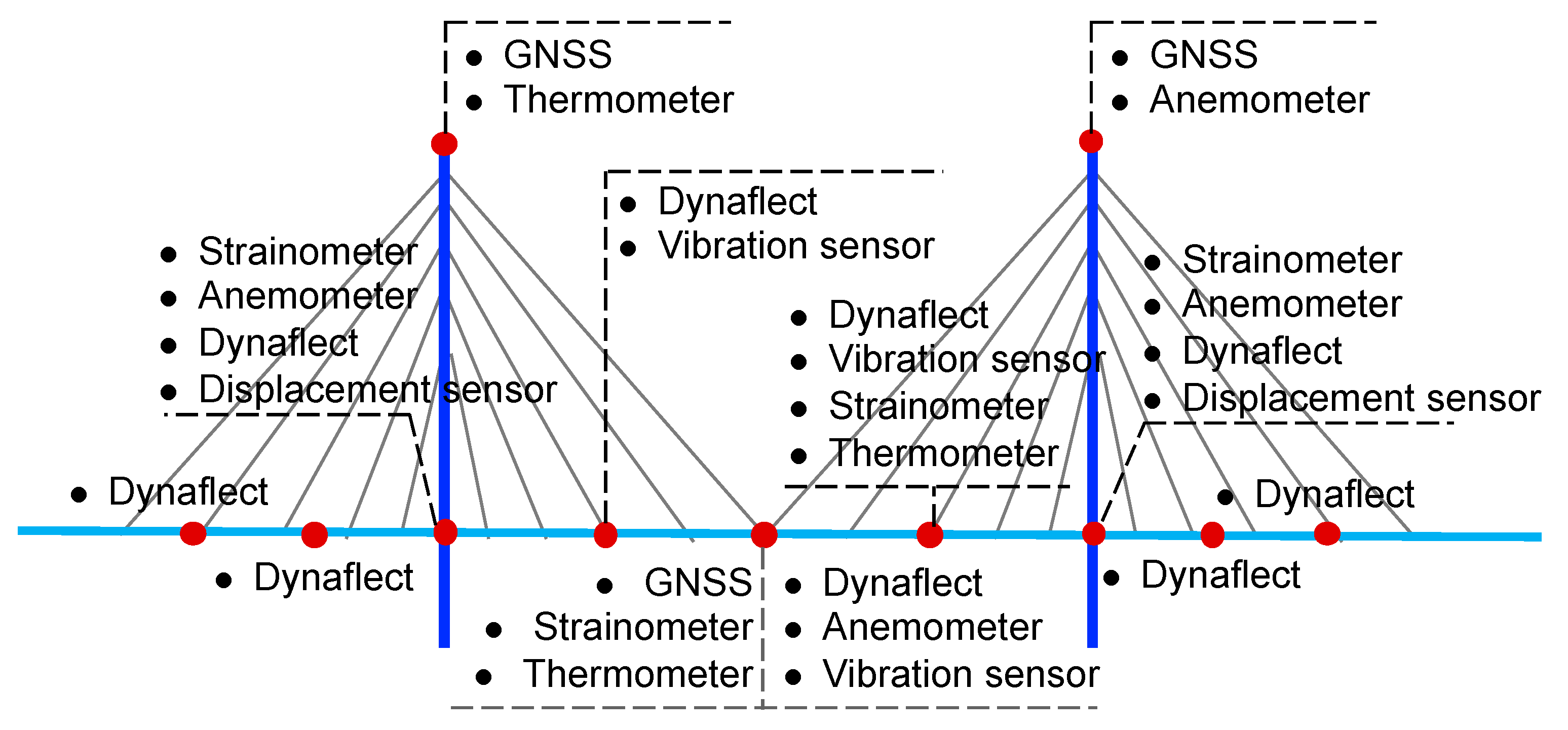
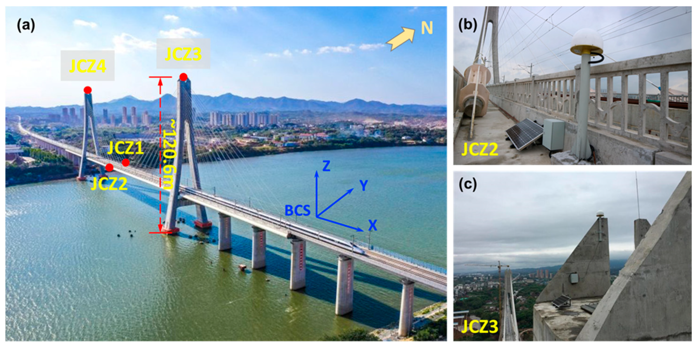
3.1. Ganjiang Bridge and SHM System

Ganjiang River Bridge in Ganzhou is located 1.9 km downstream of the confluence of Zhangshui and Gongshui rivers. The main bridge is a hybrid-beam cable-stayed bridge with a span arrangement of (35 + 40 + 60 + 300 + 60 + 40 + 35) m with a semi-floating system. Ganjiang River Bridge is the first main span of the 300 m ballastless high-speed railway cable-stay bridge in China. The horizontal and vertical deformation caused by shrinkage, creep, temperature, etc., are large and complex. At the same time, under the effects of the train swaying force, wind power, direction-finding sunshine, etc., the beam produces complex spatial deformation, and any deformation of the beam is reflected on the track, so as to affect the comfort and safety of the high-speed train operation. Therefore, a structural health monitoring system has been established in Ganjiang River Bridge to monitor the state of the bridge and systematically track it in real time and in the long term.
The sensors installed in the structural health monitoring system include: strain meter, deflection meter, GNSS, vibration sensor, pressure ring, etc., which are mainly used to monitor the bridge tower strain, static, and static strain of the main beam, the deflection of the main beam, the spatial displacement of the main beam and the bridge tower, the vibration of the main beam, and the cable force of the stayed cable. The monitoring sensors’ layout of the structural health monitoring system is shown in Figure 2. Through theoretical calculation according to the parameter of the bridge, the horizontal displacement of the beam body in the middle span of the main beam is 2.4 cm under various loading conditions of train swaying force, wind, and temperature. The maximum vertical displacement in the middle span of the main beam is 33.8 cm under the ZK live loading. Meanwhile, from the long-term monitoring data, the displacement of the bridge tower in the longitudinal direction is within 2 cm.

3.2. GNSS Data Description and Processing

GNSS receivers and antennas were installed at both sides of the bridge main span (JCZ1 and JCZ2) and the tops of the two towers (JCZ3 and JCZ4), respectively, to monitor the deformation and vibration of the middle span and the tower. The station layout is shown in Figure 3. It shows that GNSS signals of JCZ1 and JCZ2 may be blocked by surrounding objects, resulting in a serious multipath effect and affecting the accuracy and reliability of the positioning. The tower monitoring stations are located in an open-viewing environment. Therefore, their data quality may be much better than that of the main span stations. The reference station REF0 is located at the top of the project management building, and it is 1.3 km away from the bridge tower. The receivers and antennas used in this project were developed by Wuhan Navigation and LBS, and they were set to track GPS and BDS signals. The sampling rate was 5 Hz, and the cutoff elevation was 10°.
The GNSS data were processed with the homemade software called TrackGNSS v4.6.0.1, and the data processing strategies are shown in Table 1.

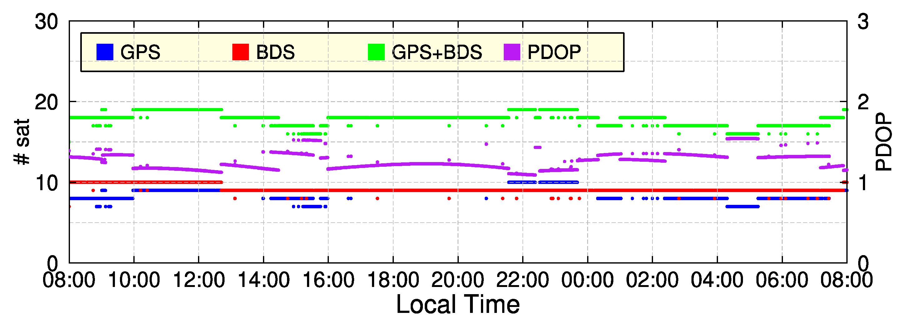
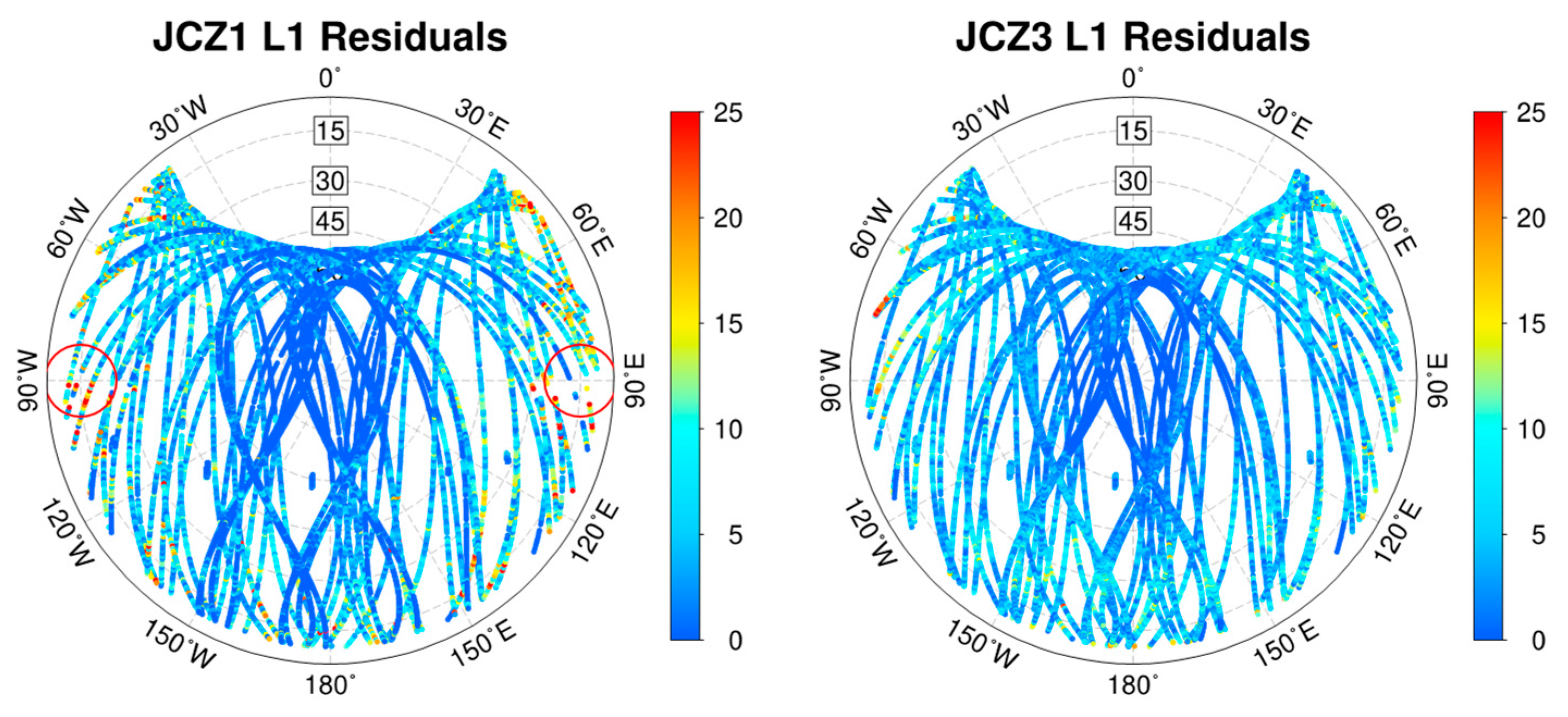
3.3. GNSS Data Quality Analysis

As previously mentioned, the distribution of GNSS satellites and the surrounding environment of the station could affect the accuracy and reliability of GNSS positioning. In Figure 4, we present the time series of the satellite visibility and PDOP on 20 May 2021. It shows that 8–10 GPS satellites and 9–10 BDS satellites can be observed for each epoch in the whole day. However, the variation in satellite numbers is relatively stable. If we use both GPS and BDS satellites to provide positioning solutions, 16–19 satellites could be used, and the PDOP is around 1.5. It demonstrates that the combination of GPS and BDS could enhance the satellite geometry to improve the availability of GNSS positioning in a harsh observing environment.
Figure 5 shows the residual sky-plot of the main span station and the tower station to demonstrate the surrounding observation environment. In the figure, the color of the round dot is the absolute value of the residuals. We can see that the residuals are normally within 1 cm, but the large residuals shown in the red cycle in the JCZ1 sky-plot are the observations contaminated by the multipath effect of the bridge tower. Therefore, the observation quality of the tower monitoring station could be much better than the main span station, and the coordinate time series could contain unreliable results, such as outliers, data interruptions, and large noises.

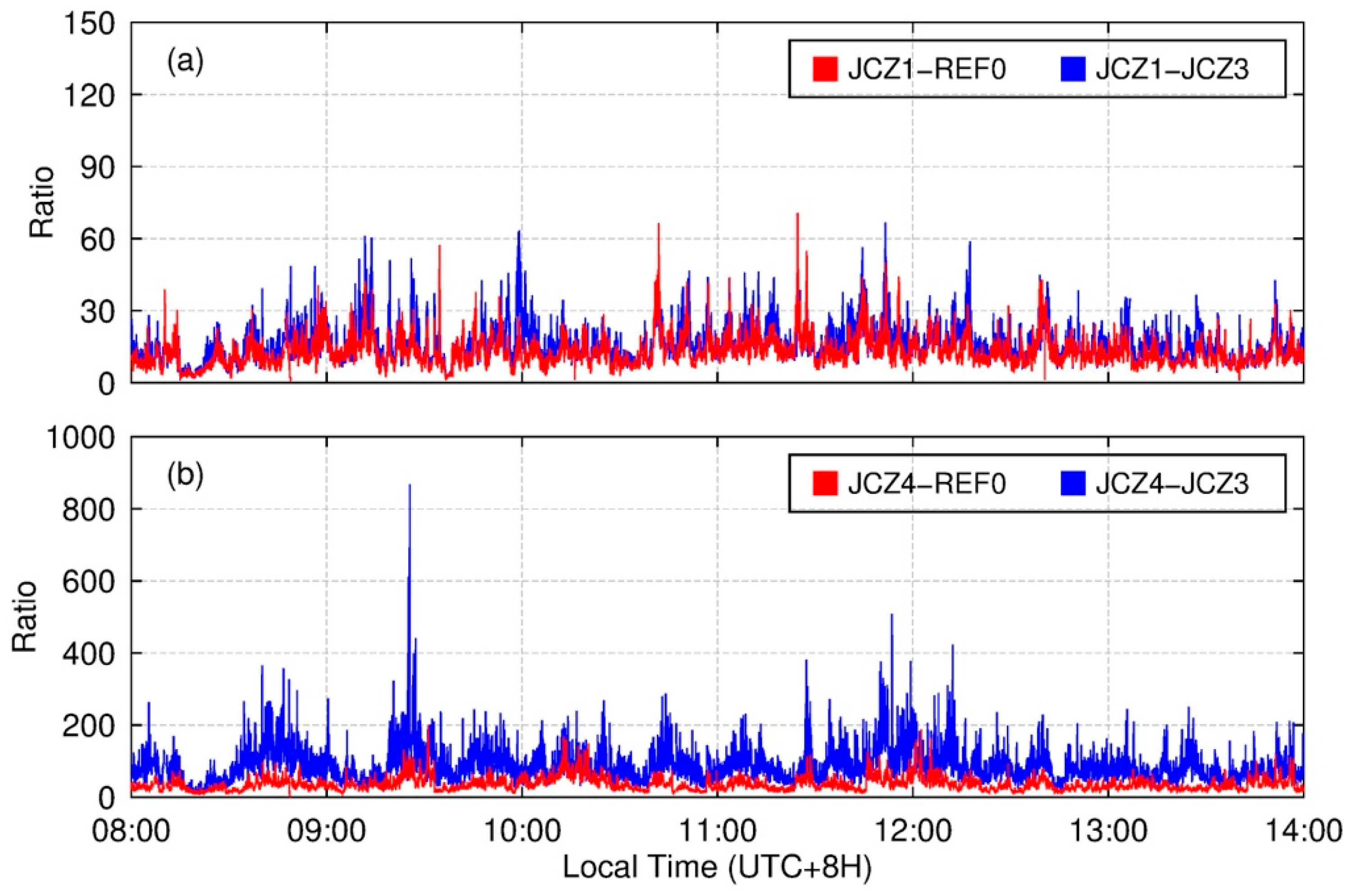
3.4. Ambiguity Resolution Performance Analysis

In GNSS data processing, the carrier phase ambiguity should be an integer value, and only the successfully fixed carrier phase ambiguity solution can achieve reliable positioning results. To evaluate the performance of ambiguity resolution of each monitoring station, Figure 6 shows the time series of ambiguity searching ratio values of the bridge mid-span and bridge tower in the single-epoch ambiguity fixed test calculated by GNSS within 6 h. In the figure, the red points denote the ratios of the ambiguity resolution for baselines with REF0 as the reference station, and the blue points are the baselines with the tower monitoring station JCZ3 as the reference station. Compared with each other, we can see that taking JCZ3 as the reference station could improve the ratio values, and the improvement could be significant for the tower stations.
Table 2 presents the statistics of the ambiguity fixing rate and the mean value of the ratio for the baseline resolution with different reference stations. It shows that the ambiguity fixing rates for all the baselines could achieve 98%, and the mean values of the ratio are higher than 12, which demonstrates the availability of GNSS positioning technology in the application of deformation and vibration monitoring of bridges. However, the baseline solutions with the reference station of JCZ3 have a higher ambiguity fixing rate and mean ratio values than those of REF0. Specifically, the ambiguity fixing rate could achieve 100% for the baseline of JCZ4–JCZ3, and the searching ratio value could be higher than 80 for every single epoch. In this case, an open-viewing observing environment could be conducive to the ambiguity resolution, and the observing condition of the reference station could play a key role in GNSS deformation monitoring applications.

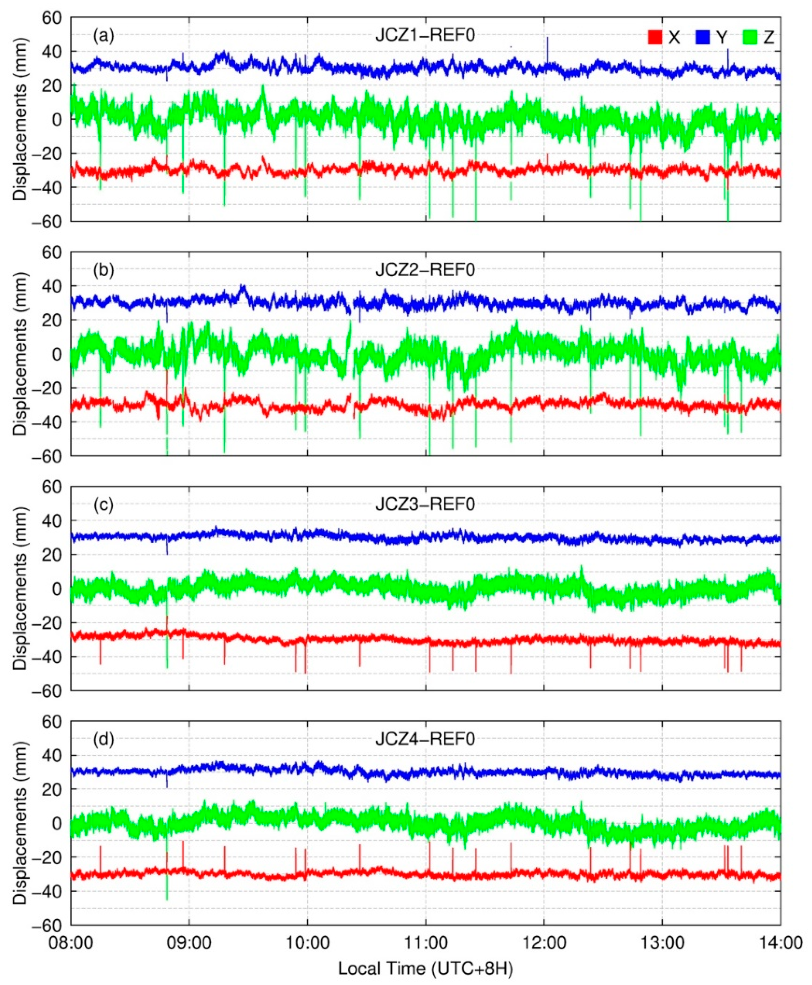
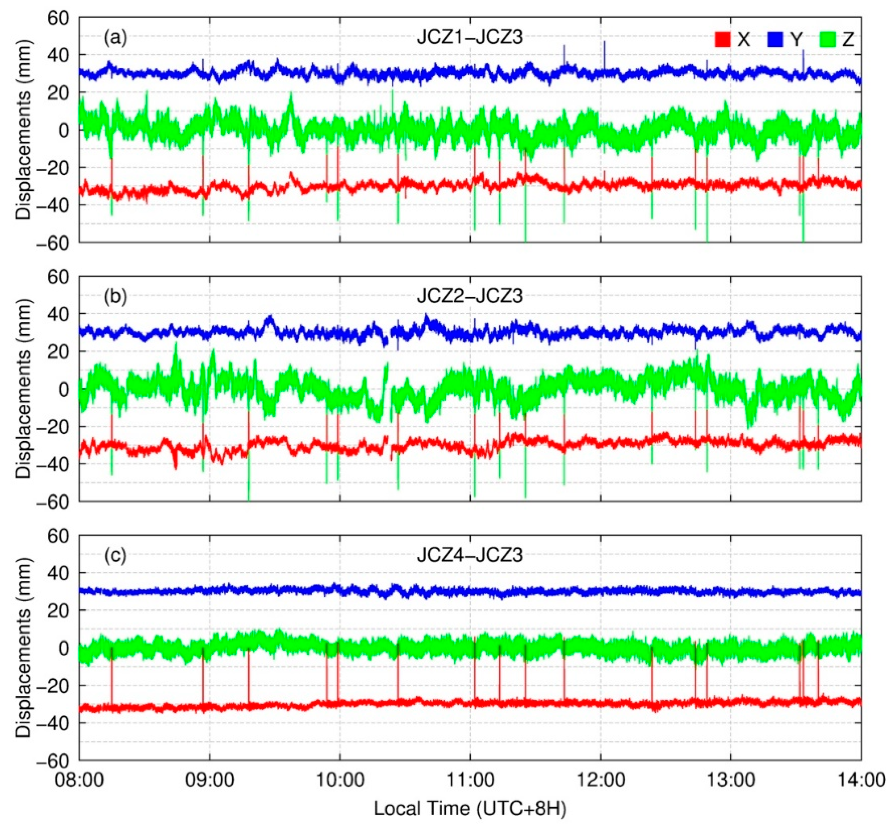
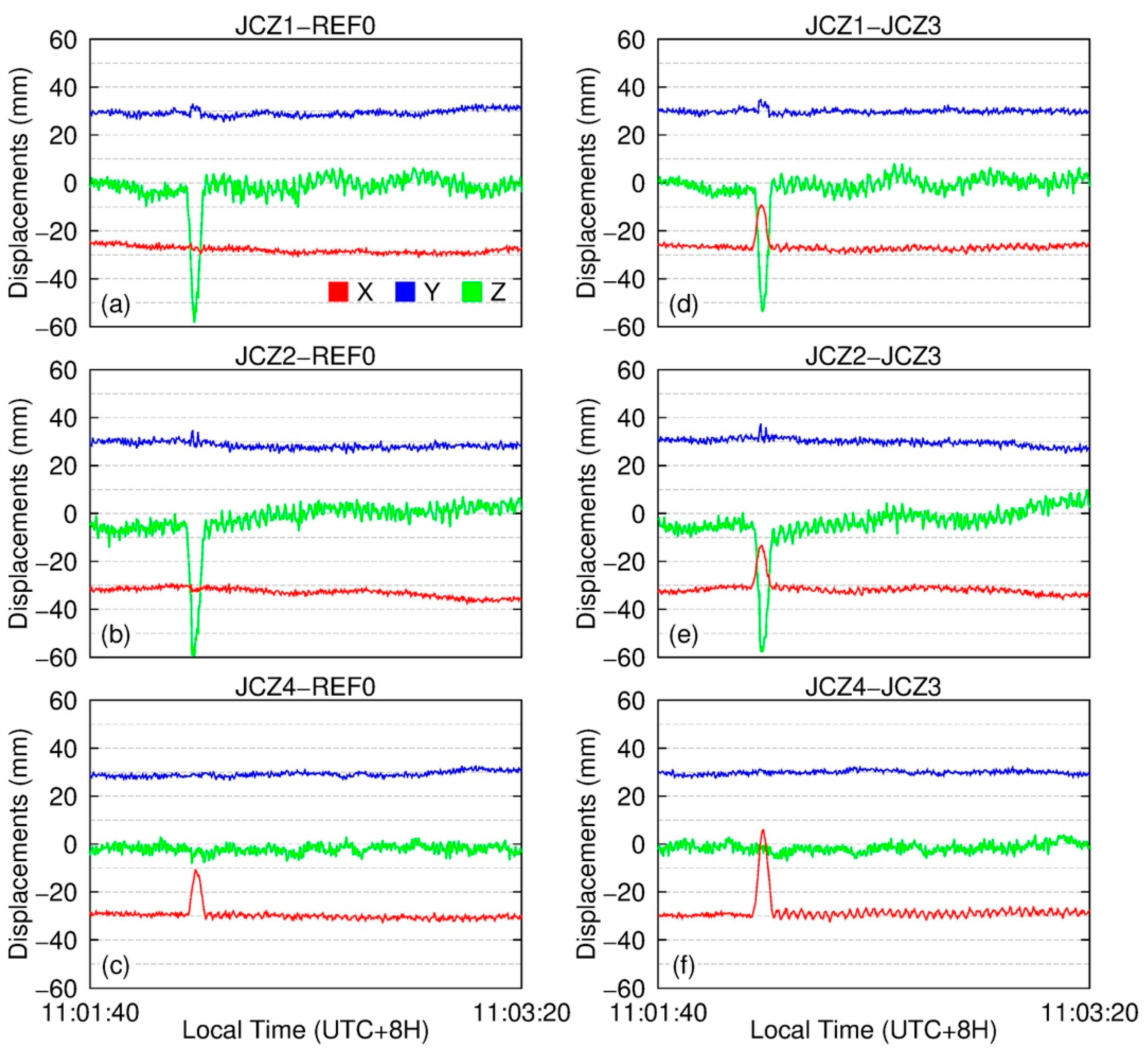
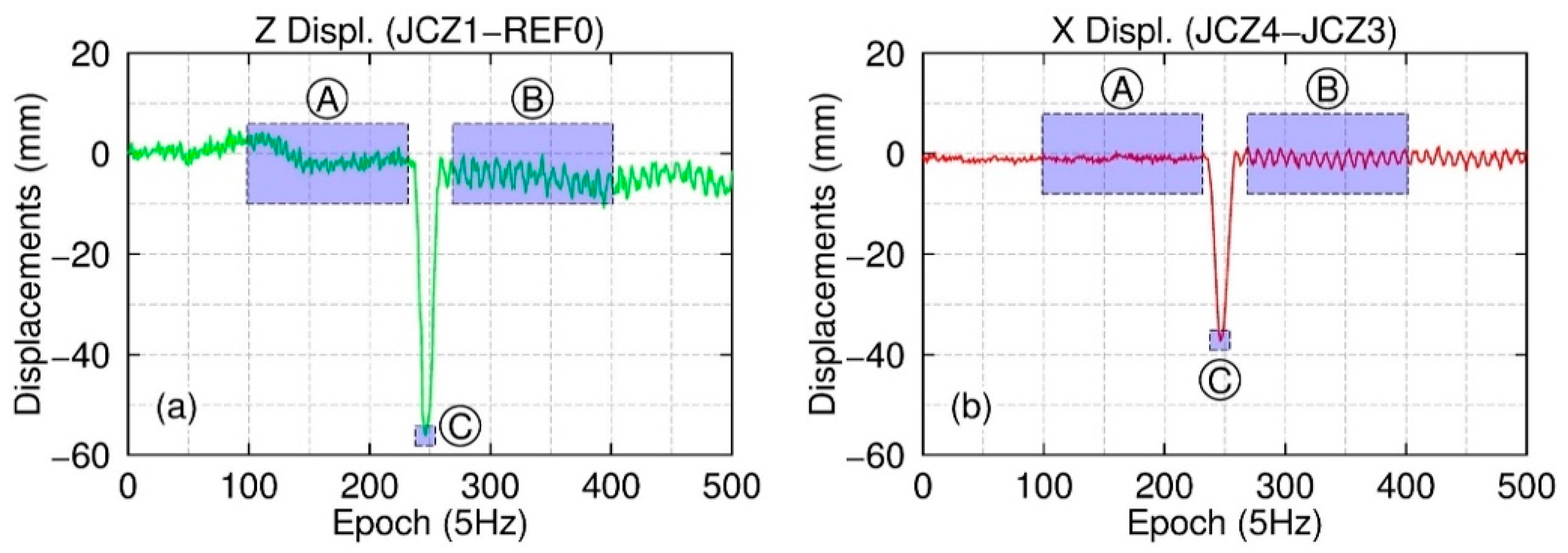
3.5. Displacement and Vibration Monitoring

Applying the above data processing methods and strategies, we processed the GNSS bridge monitoring data for 6 consecutive hours to evaluate the displacement and vibration monitoring performance of the moving-base RTK-GNSS method. Firstly, the monitoring stations are connected with REF0 to form baselines, and the coordinate time series are shown in Figure 7. In the figure, the GNSS positioning solutions have been transformed to the bridge coordinate system shown in Figure 3. Figure 8 shows the coordinate time series of baselines with the reference station JCZ3. From the two figures, we can see that significant “jumps” are evident in the X or Z direction of the time series. After careful analysis, we realized that it should be the instantaneous displacement of mid-span and tower caused by the high-speed train passing event. By tracking these “jumps”, we can precisely retrieve the moment when the train passed through the bridge.
In addition, it should be mentioned that, at the moment when the train passes through the bridge, the downward bending of the bridge deck causes the vertical deformation of the bridge’s mid-span station. Therefore, the deformation of the mid-span monitoring station is mainly reflected in the Z direction of the time series (in green). Meanwhile, at the moment when the train passes through the bridge, the two bridge towers bend towards each other, and the displacements are mainly shown in the X direction of the time series (in red). The train passing has little effect on the Y direction of the bridge. Therefore, we can distinguish outliers and displacements from the Y-direction time series (in blue).
Figure 8. Coordinate time series of each monitoring station (a): JCZ1–JCZ3, (b): JCZ2–JCZ3; (c): JCZ4–JCZ3), when the reference station is JCZ3.
Remotesensing 15 03132 g008
In Figure 8, the coordinate time series contains the motion characteristics of the two stations because JCZ3 was selected to be the reference station. This shows that the coordinate time series of JCZ1–JCZ3 and JCZ2–JCZ3 show the instantaneous bending of JCZ3 in the X direction. The downward bending of bridge deck can also be observed from the Z direction of the time series. For the bridge tower time series, due to JCZ4 and JCZ3 moving in the opposite direction, the displacements observed in the X direction should be twice the deformation of each station. Meanwhile, there are no obvious variations in the Y and Z directions.
Figure 9 presents a high-speed train passing case at 11:01:40 and 11:03:20 on 20 May 2021. The coordinate time series of baselines with REF0 as the reference station are shown in Figure 9a–c, and JCZ3 is shown in Figure 9d–f. We can see that the downward bending displacement of the bridge deck caused by the train load is about 5~6 cm, and there is only a small disturbance in the horizontal direction. Figure 9c shows that the bending of tower is about 2 cm when the train passes through the bridge, and a weak vibration signal can also be observed. In Figure 9d,e, the downward bending displacement of the bridge deck and bending of the tower can be clearly observed, and the displacement amplitude agrees well with that of the displacement shown in Figure 9a–c. In addition, in Figure 9f, not only can the double displacement caused by the tower bending be observed, but the vibration signal can also be clearly seen after the train passes the bridge. The amplitude of the vibration is around 2 mm. This means that connecting the tower stations to a baseline is conducive to capturing the vibration signal of the towers, and more importantly, the kinematic positioning precision of GNSS technology can achieve 1 mm to capture the 2 mm movement of the moving carrier. In the following, we will extract and estimate the displacement and vibration signals to evaluate the performance of moving-base RTK-GNSS method in bridge structural monitoring in detail.

4. Discussion

4.1. Displacement Estimation

In a high-speed train passing case, we can split it into three phases: before the train passes, the moment the train passes, and after the train passes. Figure 10 shows the time series of the bridge mid-span and the tower in these three phases. Take the mid-span time series as an example. Before the train passes through the bridge, there is no obvious deformation, and the time series should fluctuate around a fixed value or have a low-frequency signal accompanied by high-frequency noise. At the moment the train passes through the bridge, the middle span drops in the Z direction, and the time series returns to its initial value when the train is about to completely pass the middle span. After the train completely passes the bridge, the mid-span Z-direction time series vibrates periodically at a certain frequency around the original fixed value [42,43]. In the same way, the deformation process in the X direction of the bridge tower is similar to that of the bridge mid-span in the Z direction. To explore the movement characteristics of the bridge before and after the passage of the train, the deformation and vibration signals should be extracted from the time series. Therefore, we proposed a peak-picking method to extract the displacement from the time series for the bridge’s forced movement period [2].
From Figure 10, it can be found that the displacement time series during the train passing are similar to a wave crest or a wave trough. Therefore, we proposed to detect the train passing events using the findpeaks module from the MATLAB software. To improve the success rate of the train passing event detection, the minimum peak prominence and half-height width were set to 2 cm and 20 epochs in the findpeaks module, respectively. After the location of the wave crest or wave trough was found, the displacement time series before and after the train passing was obtained by taking several epochs before and after the wave crest or wave trough.
To accurately calculate the vertical deformation of the bridge and the longitudinal deformation of the bridge tower under the load of a high-speed rail passing, we calculated the average values of the time series before and after the train passing. Then, the bending displacements could be obtained using the following equation,
D = 1 2 1 n i = 1 n A i + 1 n i = 1 n B i 1 m i = 1 m C i ,
where the A, B and C correspond to the phases of before, after, and during the train passing, respectively. n and m are the number of samples in each phase. Following the proposed method, we firstly calculated the bending displacements of the bridge deck in the Z direction and those of the bridge tower in the X direction when the reference stations were REF0 and JCZ3. Then, we obtained the statistics of the RMSs of the results comparison, as shown in Table 3. The figure shows that the baseline resolution referenced by JCZ3 can precisely reflect the bending displacement of the bridge deck and tower, and the RMS statistics are better than 4 mm.

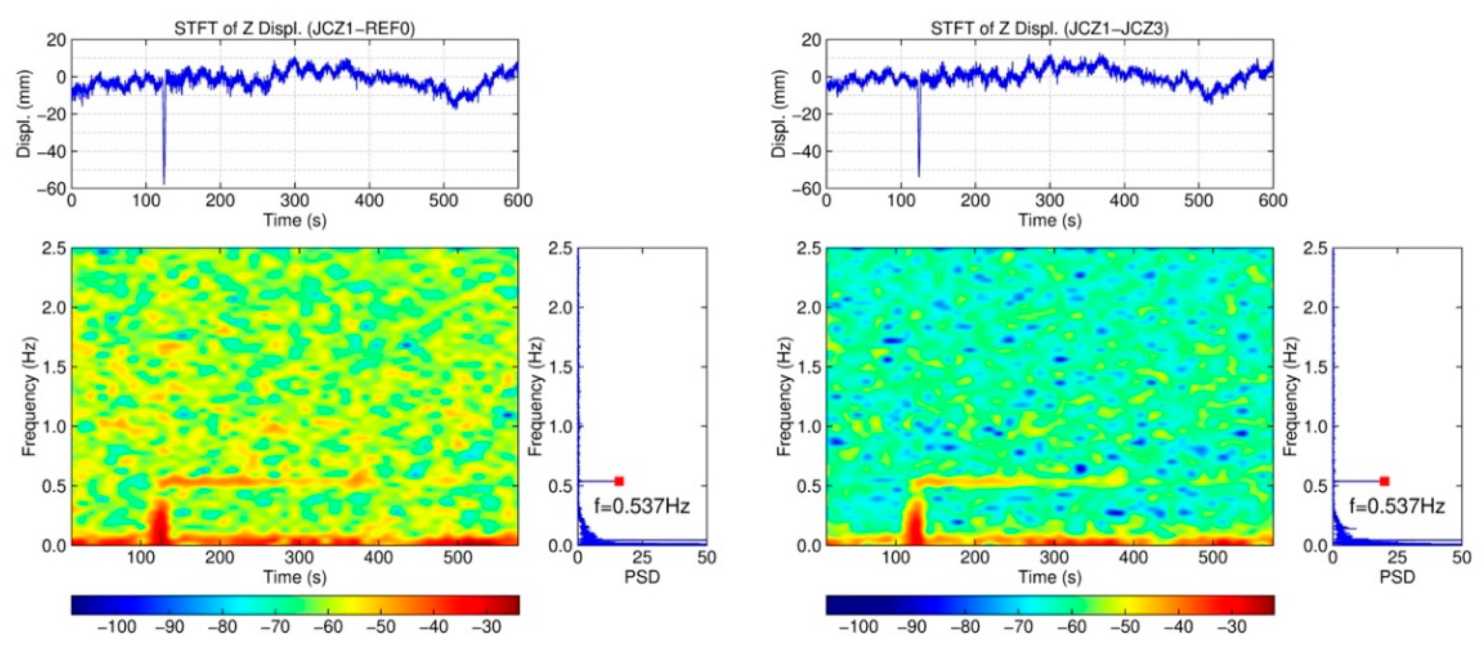
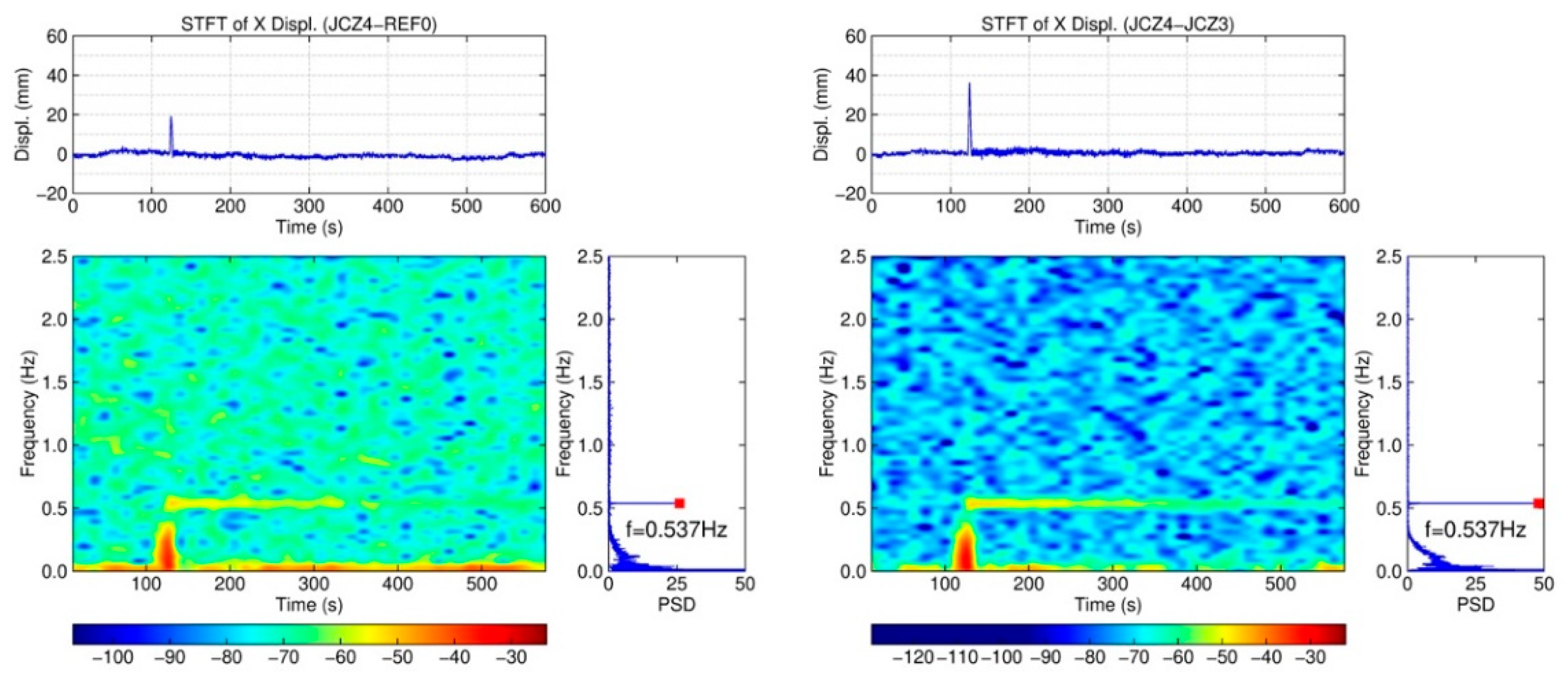
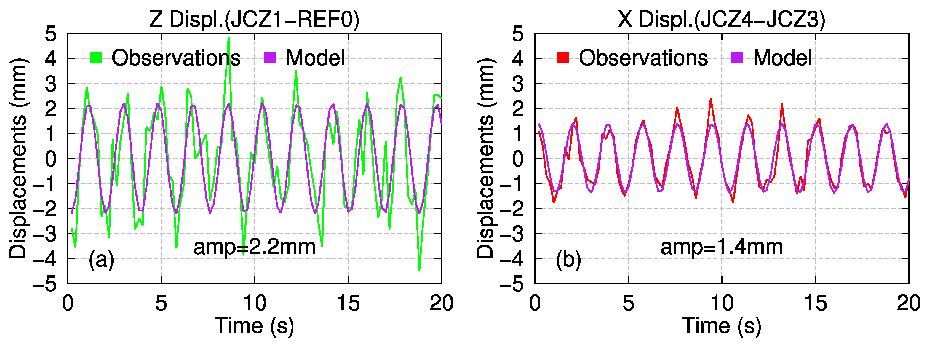
4.2. Vibration Signal Estimation

After the passing of the train, vibration could happen for the deck and tower of the bridge. Figure 11 and Figure 12 show the time series, the FFT spectral analysis, and the short-time Fourier transform (STFT) of the deck and tower vibration caused by a case of high-speed train passing. From the figures, we can see that, after the passing of the train, a vibration signal at 0.537 Hz is significant in both the bridge deck and the tower time series. The vibration frequency is exactly consistent with the theoretical vertical vibration fundamental frequency calculated using the Finite Element Model (FEM). According to the short-time Fourier transform results, the noise level of the bridge mid-span monitoring station is mainly concentrated in the low-frequency section (lower than 0.15 Hz), and the noise level in the 0.8–1.5 Hz band is high. Therefore, the vibration signal of the bridge mid-span monitoring station can easily be submerged by noise, which is not conducive to the extraction of the vibration signal. However, the vibration signal at 0.537 Hz is obvious in the deformation time series of the tower station, and the noise level is low in all frequency bands. The vibration is even better for the tower baseline solutions than for the other results. In addition, it can be seen from the short-time Fourier transform results of the bridge tower time series that the vibration signal of this frequency lasts about 470 s (about 7.8 min) from the generation to the gradual weakening to the noise level. In this study, we carried out the FFT spectral analysis for all the train passing cases on 20 May 2021, and found that the vibration frequencies were all around 0.537 Hz. The frequency is an important index in bridge structure monitoring.
We then proposed to estimate the vibration amplitude using the least-square method. Due to the damping effect of the bridge, the amplitude of the vibration gradually decreases with time until the vibration stops. To obtain the maximum vibration amplitude of the bridge after excitation, we only estimated the amplitude in a relatively short period after the train passed through the bridge’s middle span.
If the length of the time series is q , the time series can be expressed as
y i = k = 1 q a k cos ω k t i + b k sin ω k t i ,
where i is the number of epochs; t denotes the time of the epoch; k is the number of the waves in the time series; ω k is the angular frequency and can be calculated by ω k = 2 π f k ; f k is the frequency of the wave; and a k and b k are the amplitude of the sine and cosine function. We can express Equation (16) in a matrix as
E y = k = 1 q A k x k , D y = Q y ,
then, A k is the coefficient matrix of ω k and x k indicates the estimated parameters
A k = cos ω k t 1 sin ω k t 1 cos ω k t 2 sin ω k t 2 cos ω k t n sin ω k t n , x k = a k b k ,
Then, we applied the least-squares method and equal weight principle to estimate the parameters, resulting in
x ^ k = a ^ k b ^ k = A k T A k 1 A k T y ,
Thus, the amplitude of the vibration can be calculated as
a m p k = a ^ k 2 + b ^ k 2 ,
In Figure 13, we show the amplitudes measured by GNSS (Observations) and the amplitudes estimated with the method mentioned above (Model) of the vibration signals of the bridge mid-span and tower.
In the same way, we estimated the vibration amplitudes of all the 16 train passing events with the REF0 and JCZ3 referenced baseline solutions, respectively. Then, we compared the estimated amplitudes and show the RMSs in Table 4. It shows that the time series with JCZ3 as the reference station can extract the vibration signal of the bridge, and the precision is better than 1 mm. However, maybe the amplitude of the tower is relatively small (for little than 1 mm); the RMSs of the tower amplitudes lower than 1 mm are not shown in Table 4.

5. Conclusions

In bridge deformation monitoring applications, the observing condition of the reference station is not always good enough to provide high-precision positioning results. The running of the GNSS deformation monitoring system relies heavily on the reference station. In addition, for the long baselines, the double-difference technique may not be able to effectively eliminate the ionospheric or tropospheric effect errors, making it difficult to ensure the millimeter-level positioning accuracy of GNSS.
To overcome these problems, we proposed a method to take the bridge tower monitoring station as a moving-base station to build the baselines with other monitoring stations and use the moving-base RTK-GNSS method to realize the relative positioning. The moving-base RTK-GNSS model is derived and verified using the GNSS monitoring data of the Ganzhou dedicated high-speed railway bridge. The results show that the ambiguity-fixing rate can be improved by using the moving-base RTK-GNSS method with the tower monitoring station as the reference station. Specifically, the ambiguities of the moving baseline JCZ4–JCZ3 could be even fully fixed, and it is much easier to find the correct integer ambiguities from the ambiguity candidates when the tower monitoring station was selected to be a moving-base station. Meanwhile, the deformation and vibration characteristics of each monitoring point can be reflected from the time series of the moving base solutions, and the displacement and vibration amplitude estimation accuracy can achieve better than 4 mm.
Therefore, the moving-base RTK-GNSS method can be used as an alternative scheme when the observation environment of the base station is poor or the banded engineering monitoring is applied, so as to improve the monitoring capability of GNSS.

Author Contributions

Conceptualization, R.X. and W.J.; methodology, R.X.; software, W.X. and J.Y.; validation, D.X. and L.H.; formal analysis, J.M.; investigation, R.X.; resources, W.X.; data curation, J.M.; writing—original draft preparation, R.X.; writing—review and editing, W.X.; visualization, J.Y.; supervision, W.J., D.X., and L.H.; project administration, J.M.; funding acquisition, R.X., W.J., and D.X. All authors have read and agreed to the published version of the manuscript.

Funding

This research was funded by the Sanya Science and Education Innovation Park of Wuhan University of Technology (No: 2022KF0002); Hainan Province Science and Technology Special Fund Program (No: ZDKJ2021024); the Fundamental Research Funds for the Central Universities (WUT: 2022IVA035); the National Key Research and Development Program of China (No: 2021YFC3100604); and the Major Science and Technology Program for Hubei Province (No: 2022AAA002).

Data Availability Statement

The data that support the findings of this study are available from the first author, Ruijie Xi, upon reasonable request.

Conflicts of Interest

The authors declare no conflict of interest.

References

  1. Lovse, J.W.; Teskey, W.F.; Lachapelle, G.; Cannon, M.E. Dynamic Deformation Monitoring of Tall Structure Using GPS Technology. J. Surv. Eng. 1995, 121, 35–40. [Google Scholar] [CrossRef]
  2. Meng, X.; Dodson, A.; Roberts, G.W. Detecting bridge dynamics with GPS and triaxial accelerometers. Eng. Struct. 2007, 29, 3178–3184. [Google Scholar] [CrossRef]
  3. Psimoulis, P.A.; Stiros, S.C. Experimental assessment of the accuracy of GPS and RTS for the determination of the parameters of oscillation of major structures. Comput. Aided Civ. Infrastruct. Eng. 2008, 23, 389–403. [Google Scholar] [CrossRef]
  4. Martín, A.; Anquela, A.B.; Dimas-Pagés, A.; Cos-Gayón, F. Validation of performance of real-time kinematic PPP. A possible tool for deformation monitoring. Measurement 2015, 69, 95–108. [Google Scholar] [CrossRef] [Green Version]
  5. Ashkenazi, V.; Dodson, A.H.; Moore, T.; Roberts, G.W. Real time OTF GPS monitoring of the Humber Bridge. Surv. World 1996, 4, 26–28. [Google Scholar]
  6. Ashkenazi, V.; Roberts, G.W. Experimental monitoring of the Humber Bridge using GPS. Proc. Inst. Civ. Eng.—Civ. Eng. 1997, 120, 177–182. [Google Scholar] [CrossRef]
  7. Guo, J.; Xu, L.; Dai, L.; Mcdonald, M.; Wu, L.; Li, Y. Application of the real-time kinematic global positioning system in bridge safety monitoring. J. Bridge Eng. 2005, 10, 163–168. [Google Scholar] [CrossRef]
  8. Meng, X.; Roberts, G.W.; Dodson, A.H.; Cosser, E.; Barnes, J.; Rizos, C. Impact of GPS satellite and pseudolite geometry on structural deformation monitoring: Analytical and empirical studies. J. Geod. 2004, 77, 809–822. [Google Scholar] [CrossRef]
  9. Han, H.; Wang, J.; Meng, X.; Liu, H. Analysis of the dynamic response of a long span bridge using GPS/accelerometer/anemometer under typhoon loading. Eng. Struct. 2016, 122, 238–250. [Google Scholar] [CrossRef]
  10. Yi, T.; Li, H.; Gu, M. Experimental assessment of high-rate GPS receivers for deformation monitoring of bridge. Measurement 2013, 46, 420–432. [Google Scholar] [CrossRef]
  11. Wang, J.; Meng, X.; Qin, C.; Yi, J. Vibration frequencies extraction of the Forth road bridge using high sampling GPS data. Shock Vib. 2016, 2016, 9807861. [Google Scholar] [CrossRef] [Green Version]
  12. Yu, J.; Yan, B.; Meng, X.; Shao, X.; Ye, H. Measurement of bridge dynamic responses using network-based real-time kinematic GNSS technique. J. Surv. Eng. 2016, 142, 04015013. [Google Scholar] [CrossRef]
  13. Xi, R.; Chen, H.; Meng, X.; Jiang, W.; Chen, Q. Reliable dynamic monitoring of bridges with integrated GPS and BeiDou. J. Surv. Eng. 2018, 144, 04018008. [Google Scholar] [CrossRef]
  14. Xi, R.; Meng, X.; Jiang, W.; An, X.; Chen, Q. GPS/GLONASS carrier phase elevation-dependent stochastic modelling estimation and its application in bridge monitoring. Adv. Space Res. 2018, 62, 2566–2585. [Google Scholar] [CrossRef]
  15. Meng, X.; Nguyen, D.; Xie, Y.; Owen, J.; Psimoulis, P.; Ince, S.; Chen, Q.; Ye, J.; Bhatia, P. Design and implementation of a new system for large bridge monitoring—GeoSHM. Sensors 2018, 18, 775. [Google Scholar] [CrossRef] [Green Version]
  16. Meng, X.; Nguyen, D.; Owen, J.; Xie, Y.; Psimoulis, P.; Ye, G. Application of GeoSHM System in Monitoring Extreme Wind Events at the Forth Road Bridge. Remote Sens. 2019, 11, 2799. [Google Scholar] [CrossRef] [Green Version]
  17. Zumberge, J.F.; Heflin, M.B.; Jefferson, D.C.; Watkins, M.M.; Webb, F.H. Precise point positioning for the efficient and robust analysis of GPS data from large networks. J. Geophys. Res. 1997, 102, 5005–5017. [Google Scholar] [CrossRef] [Green Version]
  18. Ge, M.; Gendt, G.; Rothacher, M.A.; Shi, C.; Liu, J. Resolution of GPS carrier-phase ambiguities in precise point positioning (PPP) with daily observations. J. Geod. 2008, 82, 389–399. [Google Scholar] [CrossRef]
  19. Li, X.; Zhang, X.; Ge, M. Regional reference network augmented precise point positioning for instantaneous ambiguity resolution. J. Geod. 2011, 85, 151–158. [Google Scholar] [CrossRef]
  20. Liu, T.; Zhang, B.; Yuan, Y.; Zha, J.; Zhao, C. An efficient undifferenced method for estimating multi-GNSS high-rate clock corrections with data streams in real time. J. Geod. 2019, 93, 1435–1456. [Google Scholar] [CrossRef]
  21. Yigit, C.O.; El-Mowafy, A.; Dindar, A.A.; Bezcioglu, M.; Tiryakioglu, I. Investigating Performance of High-Rate GNSS-PPP and PPP-AR for Structural Health Monitoring: Dynamic Tests on Shake Table. J. Surv. Eng. 2020, 147, 1–14. [Google Scholar] [CrossRef]
  22. Geng, J.; Meng, X.; Dodson, A.H.; Ge, M.; Teferle, F.N. Rapid re-convergences to ambiguity-fixed solutions in precise point positioning. J. Geod. 2010, 84, 705–714. [Google Scholar] [CrossRef] [Green Version]
  23. Guo, J.; Zhang, Q.; Li, G.; Zhang, K. Assessment of multi-frequency PPP ambiguity resolution using Galileo and BeiDou-3 signals. Remote Sens. 2021, 13, 4746. [Google Scholar] [CrossRef]
  24. Wübbena, G.; Schmitz, M.; Bagge, A. PPP-RTK: Precise point positioning using state-space representation in RTK networks. In Proceedings of the ION GNSS 2005, Long Beach, CA, USA, 13–16 September 2005. [Google Scholar]
  25. Teunissen, P.; Khodabandeh, A. Review and principles of PPP-RTK methods. J. Geod. 2015, 89, 217–240. [Google Scholar] [CrossRef]
  26. Li, P.; Zhang, X.; Ren, X.; Zuo, X.; Pan, Y. Generating GPS satellite fractional cycle bias for ambiguity-fixed precise point positioning. GPS Solut. 2016, 20, 771–782. [Google Scholar] [CrossRef]
  27. Li, Z.; Chen, W.; Ruan, R.; Liu, X. Evaluation of PPP-RTK based on BDS-3/BDS-2/GPS observations: A case study in Europe. GPS Solut. 2020, 24, 38. [Google Scholar] [CrossRef]
  28. Khodabandeh, A. Single-station PPP-RTK: Correction latency and ambiguity resolution performance. J. Geod. 2021, 95, 42–66. [Google Scholar] [CrossRef]
  29. Wang, P.; Liu, H.; Nie, G.; Yang, Z.; Wu, J.; Qian, C.; Shu, B. Performance evaluation of a real-time high-precision landslide displacement detection algorithm based on GNSS virtual reference station technology. Measurement 2022, 199, 111457. [Google Scholar] [CrossRef]
  30. Ju, B.; Jiang, W.; Tao, J.; Hu, J.; Xi, R.; Ma, J.; Liu, J. Performance evaluation of GNSS kinematic PPP and PPP-IAR in structural health monitoring of bridge: Case studies. Measurement 2022, 203, 112011. [Google Scholar] [CrossRef]
  31. Paziewski, J.; Wielgosz, P. Investigation of some selected strategies for multi-GNSS instantaneous RTK positioning. Adv. Space Res. 2017, 59, 12–23. [Google Scholar] [CrossRef]
  32. Yi, T.; Li, H.; Gu, M. Recent research and applications of GPS-based monitoring technology for high-rise structures. Struct. Control Health Monit. 2013, 20, 649–670. [Google Scholar] [CrossRef]
  33. Yu, J.; Meng, X.; Shao, X.; Yan, B.; Yang, L. Identification of dynamic displacements and modal frequencies of a medium-span suspension bridge using multimode GNSS processing. Eng. Struct. 2014, 81, 432–443. [Google Scholar] [CrossRef]
  34. Xue, C.; Psimoulis, P.; Meng, X. Feasibility analysis of the performance of low-cost GNSS receivers in monitoring dynamic motion. Measurement 2022, 202, 111819. [Google Scholar] [CrossRef]
  35. Janos, D.; Kuras, P.; Ortyl, Ł. Evaluation of low-cost RTK GNSS receiver in motion under demanding conditions. Measurement 2022, 201, 111647. [Google Scholar] [CrossRef]
  36. Wang, D.; Meng, X.; Gao, C.; Pan, S.; Chen, Q. Multipath Extraction and Mitigation for Bridge Deformation Monitoring Using a Single-Difference Model. Adv. Space Res. 2017, 60, 2882–2895. [Google Scholar] [CrossRef]
  37. Xi, R.; Meng, X.; Jiang, W.; An, X.; He, Q.; Chen, Q. A refined SNR based stochastic model to reduce site-dependent effects. Remote Sens. 2020, 12, 493. [Google Scholar] [CrossRef] [Green Version]
  38. Moschas, F.; Stiros, S. Measurement of the dynamic displacements and of the modal frequencies of a short-span pedestrian bridge using GPS and an accelerometer. Eng. Struct. 2011, 33, 10–17. [Google Scholar] [CrossRef]
  39. Moschas, F.; Stiros, S. Dynamic multipath in structural bridge monitoring: An experimental approach. GPS Solut. 2014, 18, 209–218. [Google Scholar] [CrossRef]
  40. Gümüş, K.; Selbesoğlu, M. Evaluation of NRTK GNSS positioning methods for displacement detection by a newly designed displacement monitoring system. Measurement 2019, 142, 131–137. [Google Scholar] [CrossRef]
  41. Teunissen, P.J.G. The Least-squares ambiguity decorrelation adjustment: A method for fast GPS integer ambiguity estimation. J. Geod. 1995, 70, 65–82. [Google Scholar] [CrossRef]
  42. Stiros, S.C.; Psimoulis, P.A. Response of a historical short-span railway bridge to passing trains: 3-D deflections and dominant frequencies derived from Robotic Total Station (RTS) measurements. Eng. Struct. 2012, 45, 362–371. [Google Scholar] [CrossRef]
  43. Hester, D.; Brownjohn, J.; Bocian, M.; Xu, Y. Low cost bridge load test: Calculating bridge displacement from acceleration for load assessment calculations. Eng. Struct. 2017, 143, 358–374. [Google Scholar] [CrossRef] [Green Version]
Figure 2. Sensors and points layout in the structural health monitoring system.
Remotesensing 15 03132 g002
Figure 3. GNSS Site layout of monitoring stations (a), and station photographs of JCZ2 (b) and JCZ3 (c).
Remotesensing 15 03132 g003
Figure 4. Time series of satellite visibility and PDOP on 20 May 2021.
Remotesensing 15 03132 g004
Figure 5. Residual sky-plots of JCZ1 (bridge mid-span monitoring station) and JCZ3 (bridge tower monitoring station). The red cycle in the JCZ1 sky-plot are the observations contaminated by the multipath effect of the bridge tower. The colorbar denotes absolute value of the residuals.
Remotesensing 15 03132 g005
Figure 6. Time series of ambiguity searching ratio values of the bridge mid-span (a) and bridge tower (b) in the single-epoch ambiguity-fixed test. The red and blue lines indicate the baselines referenced with REF0 and JCZ3, respectively.
Remotesensing 15 03132 g006
Figure 7. Coordinate time series of each monitoring station (a): JCZ1–REF0, (b): JCZ2–REF0; (c): JCZ3–REF0; (d): JCZ4–REF0), when the reference station is REF0.
Remotesensing 15 03132 g007
Figure 9. Coordinate time series of a high-speed train passing case at 11:01:40 and 11:03:20 on 20 May 2021. (ac) denotes the baselines with REF0 as the reference station, (df) are the baselines with JCZ3 as the reference station.
Remotesensing 15 03132 g009
Figure 10. Demonstration of the three phases in the coordinate time series of bridge mid-span (a) and tower (b) in the case of train passing event. A , B and C in the figure denote the three phases: before the train passes ( A ), the moment the train passes ( B ), and after the train passes ( C ), respectively.
Remotesensing 15 03132 g010
Figure 11. Time series, FFT spectral analysis, and short-time Fourier transform (STFT) results of the bridge deck vibration caused by a case of high-speed train passing.
Remotesensing 15 03132 g011
Figure 12. Time series, FFT spectral analysis, and short-time Fourier transform (STFT) results of the bridge tower vibration caused by a case of high-speed train passing.
Remotesensing 15 03132 g012
Figure 13. Estimated amplitudes and the fitted time series of the vibration signals of the bridge mid-span (a) and tower (b).
Remotesensing 15 03132 g013
Table 1. GNSS data processing strategies in TrackGNSS software.
Models or ParametersStrategies
ObservationsThe dual-frequency observations for different systems,
GPS: L1/L2, BDS: B1/B2.
Signals and tracking modes processedThe tracking approaches for the bands are sorted in the ascending order of selecting priority, and each tracking mode is represented by one letter:
GPS L1/L2: C S L X W
BDS B1/B2: I Q X
Cutoff elevation10°
Tropospheric and ionospheric parametersEliminated by the double-difference method
Weighting schemeElevation-dependent model with σ 2 = a 2 + b 2 / sin 2 θ , where θ presents the elevation of satellites
EphemerisBRDM combined broadcast ephemeris
Ambiguity resolutionLAMBDA method
Cycle slip detectionSD HMW and GF combination observations and DD ionosphere-free (IF) observations
EstimatorKalman Filter
Table 2. Statistics of the ambiguity fixing rate and the mean ratio values.
Reference StationFixing Base (REF0)Moving Base (JCZ3)
Ambiguity Fixing RateMean Ratio ValuesAmbiguity Fixing RateMean Ratio Values
JCZ198.79%12.92799.27%16.127
JCZ298.88%12.96298.99%15.300
JCZ399.91%37.487--
JCZ499.93%35.96210088.085
Table 3. RMS statistics of the comparison of the bending displacements of the bridge deck in Z direction and the bridge tower in X direction when the reference stations are REF0 and JCZ3.
Fixing-Base BaselineMoving-Base BaselineDirectionRMS (mm)
JCZ1–REF0JCZ1–JCZ3Z2.7
JCZ2–REF0JCZ2–JCZ3Z3.6
JCZ3–REF0JCZ1–JCZ3X1.5
JCZ3–REF0JCZ2–JCZ3X1.8
JCZ3–REF0JCZ4–JCZ3X1.8
JCZ4–REF0
Table 4. RMS statistics comparison of the estimated vibration amplitudes of the bridge deck in Z direction and the bridge tower in X direction when the reference station is REF0 and JCZ3.
Fixing-Base BaselineMoving-Base BaselineDirectionRMS (mm)
JCZ1–REF0JCZ1–JCZ3Z1.1
JCZ2–REF0JCZ2–JCZ3Z1.0
JCZ3–REF0JCZ1–JCZ3X-
JCZ3–REF0JCZ2–JCZ3X-
JCZ3–REF0JCZ4–JCZ3X-
JCZ4–REF0
Disclaimer/Publisher’s Note: The statements, opinions and data contained in all publications are solely those of the individual author(s) and contributor(s) and not of MDPI and/or the editor(s). MDPI and/or the editor(s) disclaim responsibility for any injury to people or property resulting from any ideas, methods, instructions or products referred to in the content.

