Tracking Geomagnetic Storms with Dynamical System Approach: Ground-Based Observations

Abstract

Using a dynamical systems approach, we examine the persistence and predictability of geomagnetic perturbations across a range of different latitudes and levels of geomagnetic activity. We look at the horizontal components of the magnetic field measured on the ground between 13 and 24 March 2015, at approximately 40 observatories in the Northern Hemisphere. We introduced two dynamical indicators: the extremal index $\theta$, which quantifies the persistence of the system in a particular state and the instantaneous dimension d, which measures the active number of degrees of freedom of the system. The analysis revealed that during disturbed periods, the instantaneous dimension of the horizontal strength of the magnetic field, which depends on latitude, increases, indicating that the geomagnetic response is externally driven. Furthermore, during quiet times, the instantaneous dimension values fluctuate around the state-space dimension, indicating a more stochastic and thus less predictable nature system.

1. Introduction

For centuries, navigators have recognized the directional influence of Earth’s magnetic field on a compass needle. Although this understanding continues to be important in certain settings, the field of geomagnetism has progressed far beyond its historical nautical roots. The geomagnetic field is now being used to study both the Earth’s interior and its surrounding space environment. Indeed, the variations in the Earth’s magnetic field and their spatiotemporal changes offer crucial insights into the planet’s internal dynamics, lithospheric structures, tectonic movements and the state of space weather conditions resulting from Sun–Earth interactions [1]. Furthermore, geomagnetic data support a variety of practical applications, including geophysical mapping, mineral exploration, assessing space weather conditions and mapping of geoelectric hazard [2]. To facilitate these endeavors, a network of ground-based magnetic observatories has been established across the globe to provide accurate and long-term records of magnetic-field direction and intensity at fixed locations. Currently, more than one hundred magnetic observatories produce and regularly report digital data with an acquisition cadence of at least one minute. Additionally, there are ground-based fluxgate networks called variometer networks that only measure the magnetic field’s time variation in relation to a predetermined baseline. If one is only interested in identifying the magnetic field’s temporal variations rather than its absolute value, these variometer networks, which serve as a complement to magnetic observatories, can be of excellent help.

Data collected from magnetometers on the ground have played a crucial role in advancing our understanding of space weather events due to Sun–Earth interactions. These measurements have led to significant discoveries and have been used to define the different phases of magnetic storms such as the commencement, initial, main and recovery phases and to describe the time evolution of the magnetospheric substorms at high latitudes. Indeed, magnetic storms and magnetospheric substorms are among the most intricate phenomena in space weather as they interconnect the Sun, interplanetary space, the Earth’s magnetosphere and atmosphere and sometimes even the Earth’s surface in a globally unique way [3]. The interaction between these regions is continuously driven by energy from the Sun [4]. In the near-Earth space environment, the ring current is a crucial component of geomagnetic storms. It refers to an electric current that flows westward around the Earth characterized by a toroidal shape around the Earth, situated at the equatorial plane and at altitudes ranging from approximately 10,000 to 60,000 km. It is generated through the injection of ions from both the solar wind and the Earth’s ionosphere into the inner magnetosphere [5]. The ring current’s intensity enhancements cause a reduction in the magnetic field’s horizontal component near the Earth at low latitude. The decrease in the magnetic field is recorded via ground magnetograms, which are used to create the Dst index, which is the primary measure of geomagnetic storm intensity. Indeed, based on Sydney Chapman’s hypothesis that the global decrease in the geomagnetic horizontal component is only caused by an external westward electric current system around the Earth or the ring current, the Dst index was developed as a ring current measure [6]. The general consensus today is that additional magnetospheric currents, such as the cross tail current, substorm current wedge, magnetopause current and Birkeland field-aligned currents, fluctuate during geomagnetic storms and affect the Earth’s magnetic field and, in turn, the Dst index [7,8,9]. During a geomagnetic storm, a series of interrelated magnetospheric and ionospheric processes occur, known as magnetospheric substorms [10]. These processes include severe changes in the magnetospheric tail region, partial ring currents around the Earth and strong currents that cause particle precipitation into the high-latitude auroral region. The resulting auroras heat up the upper atmosphere and enhance ionospheric conductivity, leading to intense “electrojet” currents. Magnetic observatories around the world continuously monitor these processes, providing data that are used to create global indices of activity such as the auroral electrojet AE indices [11]. Therefore, magnetic observatory data play a crucial role in monitoring global magnetic storm and substorm activity but they also provide essential data for studying some of the processes occurring in the Earth’s ionosphere and magnetosphere, validating global magnetic models and supporting large satellite missions. In recent years, it has also been realized that a significant increase in solar activity can have detrimental effects on our critical technological infrastructure such as power grids, railways, aviation, telecommunications and satellite navigation [12]. Geomagnetic storms and substorms can exacerbate the situation. Modern technology’s sensitivity to severe space weather events amplifies our susceptibility to negative impacts as society becomes increasingly reliant on technology. To improve our ability to predict space weather and reduce the impacts, it is crucial to have a better and more profound comprehension of the geomagnetic field [13]. This includes understanding its variations on different spatial and temporal scales and its relationship to the dynamics of the magnetosphere and solar–terrestrial interactions [4,14,15,16,17,18].

In this context, it is important to be able to better characterize the Earth’s magnetic field and its variations on a short time scale, that is, within the range of time scales in which the Earth’s magnetic field is sensitive to changes in the intensity of ionospheric to magnetospheric currents [19,20]. It is important, for example, to investigate whether magnetic field measurements describe a system that always has the same number of degrees of freedom over time or whether this number tends to change during geomagnetically disturbed periods [16]. When the number of degrees of freedom of a system increases, this means that many independent variables must be specified to fully describe the state of the system. In other words, the system has many modes in which it can have energy or motion and these modes must be specified to fully describe the system. This may imply greater complexity in the analysis of the system and in its mathematical description [18,21]. Additionally, systems with many degrees of freedom can be more sensitive to external fluctuations and variations, which can make them more difficult to control or predict their behavior [13]. This aspect is thus critical for all studies in which magnetic field measurements are used to forecast ground disturbances caused by space weather events. To tackle this problem, we use a recently developed methodology, based on combining concepts from dynamical systems and extreme value theory, to examine the active number of degrees of freedom (i.e., the number of independent components) and the predictability of geomagnetic perturbations at various latitudes and levels of geomagnetic activity. This approach can open novel perspectives in investigating the variability of the Earth’s magnetic field due to external source mechanisms and the response of the different current systems located at different latitudes.

2. Data

We look at the variations in the geomagnetic field observed on the ground between 13 and 24 March 2015. The chosen period is particularly intriguing because it is characterized by varying levels of geomagnetic activity. Periods of quiet can be observed, interspersed with periods of more intense geomagnetic activity, characterized by the occurrence of a geomagnetic storm at mid latitudes and different magnetic substorms at higher latitudes. The temporal trend of some geomagnetic indices, such as, for example, the SYM-H and ASY-H indices [22], which describe the geomagnetic activity in mid latitudes and the AE indices [23], which, on the other hand, describe the geomagnetic disturbance fields in high latitudes well, clearly illustrate the various geomagnetic activity occurrences that characterized the chosen period.

Figure 1 depicts the scenario well. It shows the trend of four different geomagnetic indices over the selected time interval: AL, AU, SYM-H and ASY-H, respectively. These indices, which are available from the World Data Center for Geomagnetism (WDCG), Kyoto University, Japan (http://swdcwww.kugi.kyoto-u.ac.jp/index.html, accessed on 30 March 2023) have one-minute time resolution and describe various physical processes or current systems that tend to activate and/or intensify in response to solar activity. The horizontal components of the magnetic field at six mid-latitude stations are used to calculate the SYM-H and ASY-H indices, which mainly account for the disturbances to the geomagnetic field caused by the development of the magnetospheric ring current. SYM-H is similar to Dst. They are calculated in similar but not identical ways. SYM-H has the distinct advantage of having a 1 min time resolution as opposed to Dst’s 1 h time resolution [24,25]. However, while the SYM-H index describes geomagnetic disturbances at mid latitudes longitudinally symmetric to the dipole axis, the ASY-H index describes the disturbance on the horizontal component after the symmetrical part is subtracted from the disturbance field. The AU and AL indices, which are derived from horizontal variation of the geomagnetic field observed at selected (10–13) stations along the auroral zone in the Northern Hemisphere, are defined as the upper (AU) and lower envelopes (AL) of the superposed plots of all the data from these stations as functions of universal time (UT). They are used as a proxy for auroral activity because they are an indirect measure of the intensity of the auroral electrojets moving eastward and westward, respectively. The values assumed by these indices between 13 and 24 March 2015 reveal the existence of days with low geomagnetic activity (from 13 to 16 March 2015), based on the low values of the SYM-H index (above −10 nT), days with high geomagnetic disturbance (from 17 to 20 March 2015),which includes the well-known magnetic storm of 17 March 2015, also known as the St. Patrick’s Day storm, and days with moderate geomagnetic activity (from 21 to 24 March 2015), characterized by the combined observations of SYM-H < −10 nT and AU, |AL| $>$ 200 nT.

In this work, we look at the geographic North (X) and geographic East (Y) components of the Earth’s magnetic field in the geodetic reference frame, as measured via magnetometers at permanent observatories and magnetometer stations located in the Northern Hemisphere. When using magnetic data recorded on the ground, it is known that the distribution of the selected stations is uneven. In fact, there are large geographic gaps in the network of magnetic stations, most of which are found in oceanic areas. To avoid emphasizing the uneven distribution of the magnetic stations across the Northern Hemisphere, we only choose a portion of the available stations that are located in Europe and North America. Figure 2 shows the geographical distribution of the selected stations while a list of them is shown in

Table 1. The list of geomagnetic observatories used in this work. Columns refer to the IAGA identification code (ID), Geographic Latitude and Longitude, Quasi-Dipole (QD) Magnetic Latitude and Longitude, Magnetic Local Time (MLT) and the database source (I: INTERMAGNET, S: SuperMAG).

	Geographic Coordinates		QD Magnetic Coordinates
ID	Latitude (°N)	Longitude (°E)	Latitude (°N)	Longitude (°E)	MLT	Source
ABK	68.36	18.82	65.55	100.43	1.49	I
ARS	56.43	58.57	53.15	132.50	3.62	I
BEL	51.84	20.79	47.73	96.01	1.19	I
BLC	64.32	263.99	72.70	−28.02	16.92	I
BOX	58.07	38.23	54.64	113.22	2.34	I
BRD	49.87	260.03	58.73	−31.47	16.69	I
FCC	58.76	265.91	67.66	−23.97	17.19	I
FRD	38.20	282.63	47.58	0.56	18.83	I
HLP	54.61	18.82	50.80	94.87	1.12	I
HRN	77.00	15.37	74.48	106.20	1.87	I
IQA	63.75	291.48	71.10	15.65	19.84	I
IRT	52.27	104.45	48.53	179.10	6.73	I
KIV	50.72	30.30	46.73	104.48	1.76	I
LYC	64.60	23.75	61.50	102.51	1.63	I
MGD	60.05	150.73	54.56	−138.48	9.56	I
NUR	60.51	24.66	57.18	101.68	1.57	I
OTT	45.40	284.45	54.32	3.59	19.03	I
PET	52.97	158.25	46.93	−131.25	10.04	I
RES	74.69	265.11	82.08	−31.15	16.72	I
SBL	43.93	299.99	49.42	23.24	20.34	I
SPG	60.54	29.72	57.18	106.15	1.87	I
SOD	67.37	26.63	64.30	106.32	1.88	I
STJ	47.60	307.32	51.36	31.73	20.91	I
THL	77.47	290.77	83.78	26.17	20.54	I
UPS	59.90	17.35	56.62	95.16	1.14	I
AMD	69.50	61.40	66.02	137.82	3.98	S
BJN	74.50	19.20	71.80	105.85	1.85	S
C01	42.42	276.10	52.22	−8.37	18.23	S
HOP	76.51	25.01	73.54	112.62	2.30	S
NAL	78.92	11.95	76.54	107.11	1.93	S
NOR	71.09	25.79	68.11	107.97	1.99	S
PBK	70.10	170.90	66.04	−126.90	10.33	S
RPB	66.50	273.80	74.95	−12.00	17.99	S
SOL	61.08	4.84	58.33	85.18	0.47	S
T15	46.24	275.66	55.92	−8.90	18.20	S
T29	58.30	291.80	65.80	14.96	19.79	S
T44	58.47	281.95	67.15	0.83	18.85	S
T47	62.20	284.35	70.44	4.83	19.11	S
T52	53.79	282.38	62.66	1.17	18.87	S

. Each measurement site is identified by its International Association of Geomagnetism and Aeronomy (IAGA) code and includes information such as geographical and geomagnetic coordinates, magnetic local time and the database from which data were downloaded. In detail, we considered the quasi-dipole (QD) coordinate system, which is based on magnetic apex coordinates [26].

Magnetic data with a time resolution of one minute can be downloaded at http://supermag.jhuapl.edu (accessed on 30 March 2023) for data recorded at magnetometer stations that are part of the SuperMAG global network [27] and at http://www.INTERMAGNET.org/ (accessed on 30 March 2023) for data from permanent observatories that are part of the INTERMAGNET global network of observatories. Given that INTERMAGNET data are provided in the local Cartesian coordinate system (X, Y, Z), where X is the north component, Y is the east component and Z is the vertical component, and SuperMAG [27] data are provided in the cylindrical coordinate system (H, D, Z), where H is the horizontal component, D is the magnetic declination angle and Z is the vertical component (X, Y, Z), the two magnetic datasets are standardized, expressing all the data in the reference system (X, Y, Z). To remove any spikes and find any missing data, each individual set of data was checked carefully and only interruptions of less than five minutes were replaced with linearly interpolated data.

Figure 3 and Figure 4 display an example of our dataset in which the geographic north (X) and geographic east (Y) components of the Earth’s magnetic field are presented for five different geomagnetic observatories, denoted by the corresponding IAGA identification code and located at mid to high latitudes. Some recognizable classic signatures can be seen in the temporal trends of the X and Y components, such as those connected to the occurrence of a magnetic storm and the diurnal variation during quiet periods at lower latitude observatories like KIV and UPS or to the succession of substorms in the case of recordings at the highest latitude observatories (ABK, HRN and THL).

3. Methods

We use a dynamical systems approach to characterize the persistence and the predictability of geospace perturbations at different latitudes by using the X and Y components of the Earth’s magnetic field. The idea is that the 2D vector $s\left(t\right)= [$X$\left(t\right),$Y$\left(t\right)]$ is representative of the states visited by the system, i.e., it provides an instantaneous view of the geomagnetic conditions. Clearly, this is only a “reduced” state-space that would be fully characterized only if retaining information on a large number of variables and observables, representative of the different dynamical components of the geospace environment (as, for example, the solar wind parameters). With our 2D representation, we are able to describe the geomagnetic dynamics as a sort of isolated system and to investigate if any external feedback emerges by looking at its “reduced” state-space. For this reason, we also excluded the vertical component (Z) from our analysis since it is mainly representative of the external feedback activated from interplanetary variability. However, the dynamical indicators we use in our analysis are free from any constraints on the number of selected variables and are able to represent the action of external/unknown forcing/variables unless they are not explicitly considered. In the following, we refer to the region where $s\left(t\right)$ resides as the state-space and to the trajectory $s\left(t\right)$ as the portrait in the state-space telling us how the different states evolve with time.

The mathematical basis of our approach is founded in linking the extreme value theory with the concept of recurrences introduced by Poincaré in his recurrence theorem [28]. Let $\zeta$ be a state of interest of the system, i.e., $\zeta =s\left(t^{\ast }\right)$, that corresponds to a specific geomagnetic configuration observed at the time $t^{\ast }$ for a specific geomagnetic observatory. Let us introduce the Euclidean distance $\delta \left(t\right)$ as

$$\delta \left(t\right)=\Vert \zeta -x\left(t\right)\Vert$$

(1)

where $\Vert \cdots \Vert$ stands for the norm in the ${\mathbb{L}}^2$ Hilbert space. Let $ϵ$ be a threshold related to the q-th quantile of the cumulative distribution function of $x\left(t\right)$ via the relation

$$q=e^{-ϵ}.$$

(2)

By defining

$$g\left(t\right)=-log\left(\delta \right)$$

(3)

as the logarithmic return, the probability of logarithmic returning in a circle of radius $ϵ$ centered on the state of interest $\zeta$ according to the Freitas–Freitas–Todd theorem [29] modified by Lucarini et al. [30] is a Generalized Pareto-like Distribution GPD $\left(\mu ,\sigma ,q\right)$ of the form

$$\mathrm{GPD}\left(\mu ,\sigma ,q\right)=\mathcal{P}\left(g\left(t\right)>q,\zeta \right)\simeq exp\left[\frac{x\left(t\right)-\mu }{\sigma }\right].$$

(4)

where the condition $g\left(t\right)>q$ is derived from the threshold condition $\delta <ϵ$ [31]. The GPD free parameters $\mu$ and $\sigma$ depend on the selected state $\zeta$ and can be related to the first (i.e., the mean) and the second (i.e., the variance) moments of $\mathcal{P}$, respectively, via the relations

$$\begin{array}{ccc}\mathbb{E}\left[x\right]& =& \mu +\sigma ,\end{array}$$

(5)

$$\begin{array}{ccc}\mathbb{E}\left[x^2\right]-{\left(\mathbb{E}\left[x\right]\right)}^2& =& {\sigma }^2.\end{array}$$

(6)

By requiring that the invariant measure of the system locally scales with a well-defined exponent, named local or instantaneous dimension d, a direct relation can be obtained between $\sigma$ and d as

$$d=\frac{1}{\sigma }.$$

(7)

When all available states are explored (i.e., all possible geomagnetic configurations $\zeta$ corresponding to each time instant t), an instantaneous picture of the system’s states is obtained, providing information on the active number of degrees of freedom at each t. When averaged over time $\langle d\rangle$ the classical concept of the system dimension is recovered [32,33,34]. Since the GPD parameter $\sigma >0$, then $d\in [0,+\infty ]$.

Another dynamical indicator introduced in the field of extreme value theory and dynamical systems is the so-called extremal index $\theta$, providing us information on the inverse of the residence time of the system in a specific state $\zeta$. Thus, $\theta$ is a measure of the clustering of extreme/rare events (as geomagnetic storms) in the phase-space and it allows us to discriminate between purely Poisson processes for the statistics of extreme events (when they do not cluster) and a compound Poisson process (in the presence of clustering of rare events) [35], acquiring an appealing physical meaning. For independent and identically distributed extremes $\theta =1$, while for “correlated” extremes $0<\theta <1$. Within the different methods proposed to evaluate the extremal index (e.g., [35]) in the field of dynamical systems it can be evaluated by using the Süveges maximum likelihood estimator [35,36]

$$\theta =\frac{{\sum }_{i=1}^N\rho S_i+N-1+N_c-{\left[{\left({\sum }_{i=1}^{N-1}\rho S_i+N-1+N_c\right)}^2-8N_c{\sum }_{i=1}^{N-1}\rho S_i\right]}^{1/2}}{2{\sum }_{i=1}^{N-1}\rho S_i}$$

(8)

where N is the number of observations exceeding the threshold, $\rho$ is the distribution function of the threshold, $S_i$ is the exceedance distance and $N_c={\sum }_{i=1}^{N-1}I(S_i\ne 0)$ where I is the indicator function for the selected $S_i$. We refer the reader to [36] for further details on the numerical evaluation of the extremal index. Since in the field of dynamical systems $\theta$ is a measure of the inverse of the mean residence time within the hyper-sphere of radius $ϵ$, it can be introduced in Equation (4) as

$$\mathrm{GPD}\left(\mu ,\sigma ,q,\theta \right)\simeq exp\left[-\theta \frac{x\left(t\right)-\mu }{\sigma }\right].$$

(9)

Since $\theta \in [0,1]$, the more $\theta$ increases the less persistent the state $\zeta$ is [31,35]. As for d, since we can explore all states $\zeta$ (i.e., all time instants), an instantaneous view of the residence time of the system into the different states is obtained. The instantaneous dimension d and the extremal index $\theta$ allow one to provide novel insights and an innovative view of extreme phenomena into different fields as transient events in the atmospheric circulation [37,38,39,40], in the ocean dynamics [41], transient disturbances of the geomagnetic field due to geomagnetic storms and magnetospheric substorms [16], localized energy transfers in hydrodynamic [42] and magnetohydrodynamic [43] turbulence and earthquake dynamics [44,45].

4. Results and Discussions

Figure 5 and Figure 6 show the temporal behavior of the instantaneous dimension d and the inverse persistence $\theta$ at five different observatories located at mid to high latitudes chosen as examples, the same observatories whose X and Y components are shown in Figure 3 and Figure 4.

The main feature of the behavior of the instantaneous dimensions is that larger dimensions are observed during the disturbed- and moderate-activity periods in comparison with the quiet period, regardless of magnetic latitude. This clearly reflects the externally driven nature of the geomagnetic response during active periods, increasing the active number of degrees of freedom when an interplanetary perturbation hits the Earth’s magnetopause and propagates within the magnetosphere’s inner regions [46,47]. Conversely, during quiet periods the instantaneous dimensions d fluctuate around the state-space dimension $d_s=2$ (we remark we used a 2D representation of the system by means of X and Y components) at all latitudes. This means that the system (i.e., the horizontal dynamics of the geomagnetic field) visits all parts of the state-space, thus suggesting that it cannot be reduced into smaller components and its fluctuations behave randomly. Finally, at mid latitudes, a reduction in the instantaneous dimension d is observed at the beginning of the recovery phase (end of 17 March 2015), reaching values lower than the state-space dimension $d_s$, which is perfectly in agreement with the time at which the z component of the interplanetary magnetic field $B_z$ turns off from negative values, indicating that the Earth’s magnetosphere was restored to a closed configuration. Following that, the instantaneous dimensions d tend to return to their quiet-time values (i.e., $d\simeq d_s=2$), although some larger values are observed that are representative of the different processes occurring during the recovery phase of a geomagnetic storm and involving different spatio-temporal scales as well as a wide range of physical mechanisms.

By specifically focusing on the disturbed period (from 17 to 20 March) our analysis reveals different interesting features. First of all, the timing of the largest value of the instantaneous dimension is delayed as the latitude decreases, in agreement with the faster response of the high-latitude dynamics with respect to the mid-latitude one [10,14,48]. This could also indicate a possible high-to-low-latitude coupling due to the different response time of the geospace current systems as highlighted in previous works [16,49]. Secondly, by looking at the peak values of d as a function of the latitude, we highlight that larger dimensions are found in the magnetic latitude band [60$°$, 70$°$]N with respect to both the highest and lowest latitudes, exactly matching the expected boundary of the auroral oval. This underlines that a large number of processes and phenomena take place at the boundaries of the auroral oval during the main phase of a geomagnetic storm.

By focusing instead on the period characterized by moderate geomagnetic activity (from 21 to 25 March), the most interesting feature is the sudden increases in the instantaneous dimensions observed at latitudes around 60$°$–70$°$N (see, e.g., the behavior at UPS, ABK, HRN), closely matching the sudden depressions and increases observed in the auroral indices AL and AU, respectively (see Figure 1). The close correspondence highlights again the role of the instantaneous dimension d in deciphering the timing and the spatial location of externally induced fluctuations, suggesting that the dynamics near the boundary of the auroral oval cannot be described as a low-dimensional system. We will return to this point in Section 5.

The dynamical behavior of the extremal index $\theta$ also displays an interesting and intriguing behavior, both comparing disturbed and quiet periods as well as across magnetic latitudes. The first feature that emerges is a clear 1-day variability at latitudes around 60$°$–70$°$N, as shown in Figure 6 for ABK and HRN. This can be attributed to the daily variability observed in the solar quiet (Sq) current system whose center is located at mid latitude but whose maximum variability is observed around the boundary of the auroral oval [50]. This 1-day variability is destroyed when the geomagnetic storm occurs [51], reflecting the large-amplitude short-term variability caused by the triggering activity of the solar wind external forcing [14]. Lower extremal index $\theta$ values are observed at low latitudes and in the polar cap region (e.g., THL), implying that more stable conditions are observed related to the center of the northern lobe of the Sq (at lower latitudes) and the presence of Sun-aligned arcs in the polar cap region [52]. Another interesting feature is that at the end of the main phase of the geomagnetic storm (i.e., when the minimum SYM-H value is reached) all latitudes have extremely low values of $\theta$ (i.e., $\theta \le 0.1$), indicating the overall response of the geomagnetic field variations to the strong driver induced by the solar wind. This is consistent with the delayed response time of geomagnetic activity at different latitudes when the internal response time of the magnetosphere–ionosphere system is considered [14,16,49]. Finally, larger amplitude fluctuations around the mean are observed for geomagnetic stations located at the boundary of the auroral oval as a result of the short-term high-amplitude variability of the geomagnetic field observed at these latitudes. These more unstable dynamics (i.e., larger $\theta$ values with larger fluctuations) are caused by contributions from various current systems with boundaries close to the auroral oval. Finally, unlike the instantaneous dimensions, d, the extremal index, $\theta$, cannot be used as a proxy for distinguishing the different levels of geomagnetic active periods, assuming similar values during both the disturbed and moderate periods of activity.

To better highlight latitude-dependent features during different periods of geomagnetic activity, we report the average dimensions $\langle d\rangle$ and extremal index $\langle \theta \rangle$ as a function of the Quasi-Dipole (QD) magnetic latitude for the three different activity periods (quiet, disturbed and moderate) in Figure 7.

The average instantaneous dimensions are nearly independent of geomagnetic latitude, assuming a nearly constant value, but they are sensitive to the level of geomagnetic activity. Indeed, the larger the average dimensions, the more disturbed the geomagnetic activity, rising from $\langle d\rangle \simeq 2$ during the quiet period up to $\langle d\rangle \simeq 2.3$ during the disturbed period. The average extremal index, $\langle \theta \rangle$, on the other hand, is almost independent of geomagnetic activity (though smaller values are observed during periods of increased activity), while it is dependent on geomagnetic latitude. Indeed, lower values are found at lower latitudes (i.e., $\langle \theta \rangle \simeq$ 0.1–0.2), while higher values (i.e., $\langle \theta \rangle \simeq 0.3$) are observed across the auroral oval’s boundary, 60$°$–70$°$N, with the latter slightly decreasing during the geomagnetic storm as a result of more persistent conditions caused by the external forcing from the solar wind acting as a driver of geomagnetic fluctuations [14]. However, during the disturbed period, a slight dependence on magnetic latitude of the average dimensions $\langle d\rangle$ is observed, which can be attributed to the greater number of processes and phenomena occurring at high latitudes compared to those occurring at mid latitudes. Thus, the pair $(d,\theta )$ seems to be a promising tool for investigating the geomagnetic activity, both during quiet and disturbed periods and for discerning the role of high- vs. mid-latitude processes in terms of active degrees of freedom and persistent properties.

As a final step, to further characterize the behavior across a disturbed period we show in Figure 8 the daily polar view maps of the instantaneous dimensions d and the inverse persistence $\theta$ in the Northern Hemisphere. We began by assuming that, given that any magnetic station co-rotates with the Earth, each of them moves along an ideal circumference around the pole in one day. Using magnetic stations located at various latitudes and data collected during a day, we have a good latitudinal coverage that allows us to obtain a good daily representation of instantaneous dimensions and inverse persistence. Indeed, for each day, we reduce all of the data evaluated at each chosen magnetic station to a regular grid (1.5$°$–1.5$°$) and use the weighted Gaussian interpolation scheme. This reduces the possibility of artifacts caused by a non-uniform spatial distribution of data. This method clearly smooths the available information, which is determined by the width of the weighting function, which has been set to 2.5$°$. Figure 8 displays an example of the obtained results focused on 7 days around the St. Patrick’s Day storm. Data are displayed in magnetic coordinates using a polar representation and more precisely in QD-latitude and magnetic local time (MLT) reference systems. This magnetic reference system was chosen because QD coordinates are particularly well-suited for describing horizontally stratified phenomena in the ionosphere [53] and the addition of MLT allows for data organization with respect to the Sun position. To aid interpretation of the results, Figure 8 also depicts the temporal trends of geomagnetic indices that accurately describe geomagnetic activity at various latitudes.

Analyzing the daily variation of the instantaneous dimension, its strong dependence on geomagnetic activity immediately becomes evident. On the two days of 17 and 18 March, which were characterized by the initial phases of a magnetic storm and a series of substorms as clearly indicated by the values of all geomagnetic indices shown in Figure 8, the instantaneous dimension d assumed higher values than both the preceding and following days. Almost everywhere, the value of the instantaneous dimension is around 2.4, which, considering the chosen color scale, gives both daily maps a characteristic intense blue color that is completely different from the daily maps of the preceding and following days. In those maps, the blue color is mainly confined to high latitudes, while shades of yellow and green dominate, corresponding to instantaneous dimension values between 1.9 and 2.2. If we consider that between 17 and 18 March, the formation of an intense ring current affecting the horizontal component of the magnetic field at mid latitudes was observed, along with intense auroral currents affecting the horizontal component of the magnetic field at high latitudes, this immediately explains the sudden increase in the value of the instantaneous dimension and, above all, the fact that this increase occurred on a large spatial scale, effectively involving all latitudes and local magnetic times analyzed. The intensification of these current systems, therefore, makes the system more complex to describe, requiring a greater number of degrees of freedom. As confirmation that the increase in the value of the instantaneous dimension depends mainly on the influence that current systems flowing in the ionosphere and magnetosphere have on the magnetic field, we overlaid the structure of plasma convection cells obtainable through the CS10 model [54] onto our daily maps. This is a statistical model obtained using data measured via SuperDARN (Super Dual Auroral Radar Network), a network of 35 high-frequency radars located on the ground that calculates the distribution of high-latitude plasma convection patterns organized by solar wind, interplanetary magnetic field and dipole tilt angle conditions. Thanks to the use of this model, it was possible to reconstruct the average structure of high-latitude plasma convection cells using the daily average values of solar wind and interplanetary magnetic field parameters specific to the various analyzed days. The plasma convection cells are structured along magnetic field lines and their orientation is determined by the electric field direction. Understanding the position of ionospheric current systems during the analyzed week is facilitated by the convection cells, which are driven by the auroral electrojet currents. During the main phase of the storm, the convection cells reach their maximum spatial extent. Between 16 and 17 March, corresponding to the succession of substorms at high latitudes, the convection cells expanded beyond 60$°$ magnetic latitude, then gradually contracted, extending to about 70$°$ magnetic latitude in the following days. The daily maximum values of the instantaneous dimension appear to be influenced by the evolution of the plasma convection cells, indicating a possible correlation with the presence and intensity of auroral electrojet currents.

Regarding the daily trend of the inverse persistence $\theta$, it is possible to observe that, regardless of the analyzed day, there are always three distinct zones: one for latitudes greater than 80$°$, one with latitude values between 60$°$ and 80$°$ and one with latitude values less than 60$°$. The intermediate zone is the one where the $\theta$ index takes higher values compared to the other two zones. This structure is clear on days of low or moderate activity, while it is less distinct on the two days of higher geomagnetic activity. On 16 and 17 March, the intermediate zone appears to narrow, leaving room for an expansion of the other two zones, resulting in a general decrease in the $\theta$ index value. Not only is the intermediate zone characterized by higher average values of the $\theta$ index, but the values assumed by the $\theta$ index in the other two zones tend to be lower than on other days. As a result, the intensification of ionospheric and magnetospheric currents, which have a strong effect on the magnetic field at different latitudes, ultimately leads to a decrease in the $\theta$ index on a global scale. This indicates that the system has a tendency to become more globally stable and persistent under the influence of fully developed ionospheric and magnetospheric dynamics.

5. Conclusions

In this study we reported the characterization of the horizontal dynamics of the geomagnetic field during disturbed, moderate and quiet periods of geomagnetic activity by using recent advancements in the field of dynamical systems and extreme value theory. In particular, we used two dynamical indicators: the instantaneous dimension d, measuring the active number of degrees of freedom of the system and the extremal index $\theta$, quantifying the persistence of the system in a particular state. Our analysis revealed that during disturbed periods, the instantaneous dimensions increase, indicating the externally driven nature of the geomagnetic response. Conversely, during quiet periods, the instantaneous dimensions fluctuate around the state-space dimension, suggesting an ergodic (more stochastic, less predictable) nature of the system.

The main results of the paper can be summarized as follows.

• The dynamics of the auroral oval are that it is not a low-dimensional one, thus suggesting that this specific region cannot be described by a reduced number of degrees of freedom (i.e., variables). This result can only be highlighted by looking at ground-based geomagnetic observatories (instead of geomagnetic indices) to explore the associated latitudinal band and can be highlighted only by using a methodology that is free from any constriction on the number of observables used for the analysis. Indeed, previous results [55,56], although robust, were based on selecting a specific (embedding) dimension m and those metrics cannot be characterized by values larger than m, thus forbidding access to information on the possible unknown variables that are not included in the analysis.
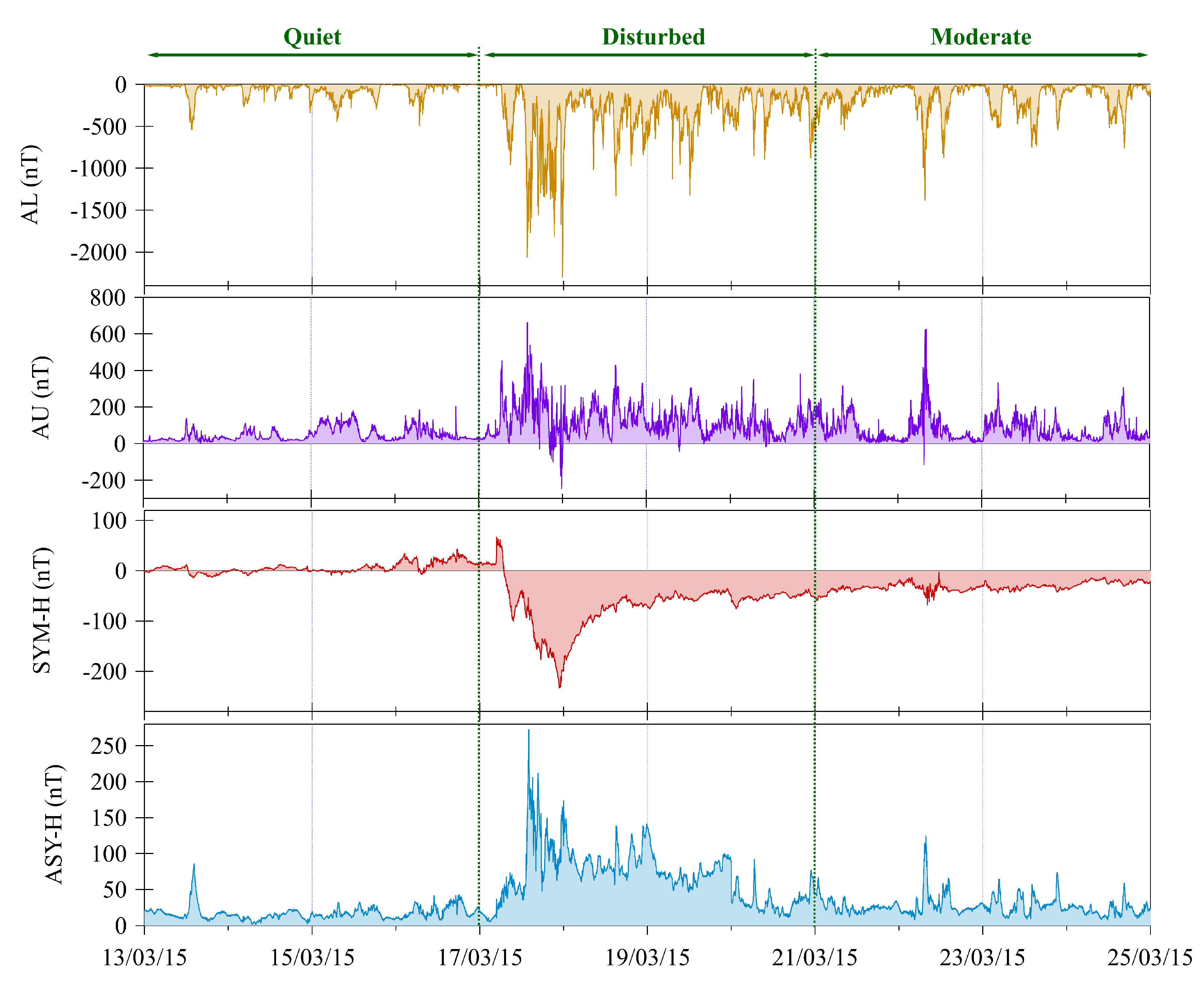
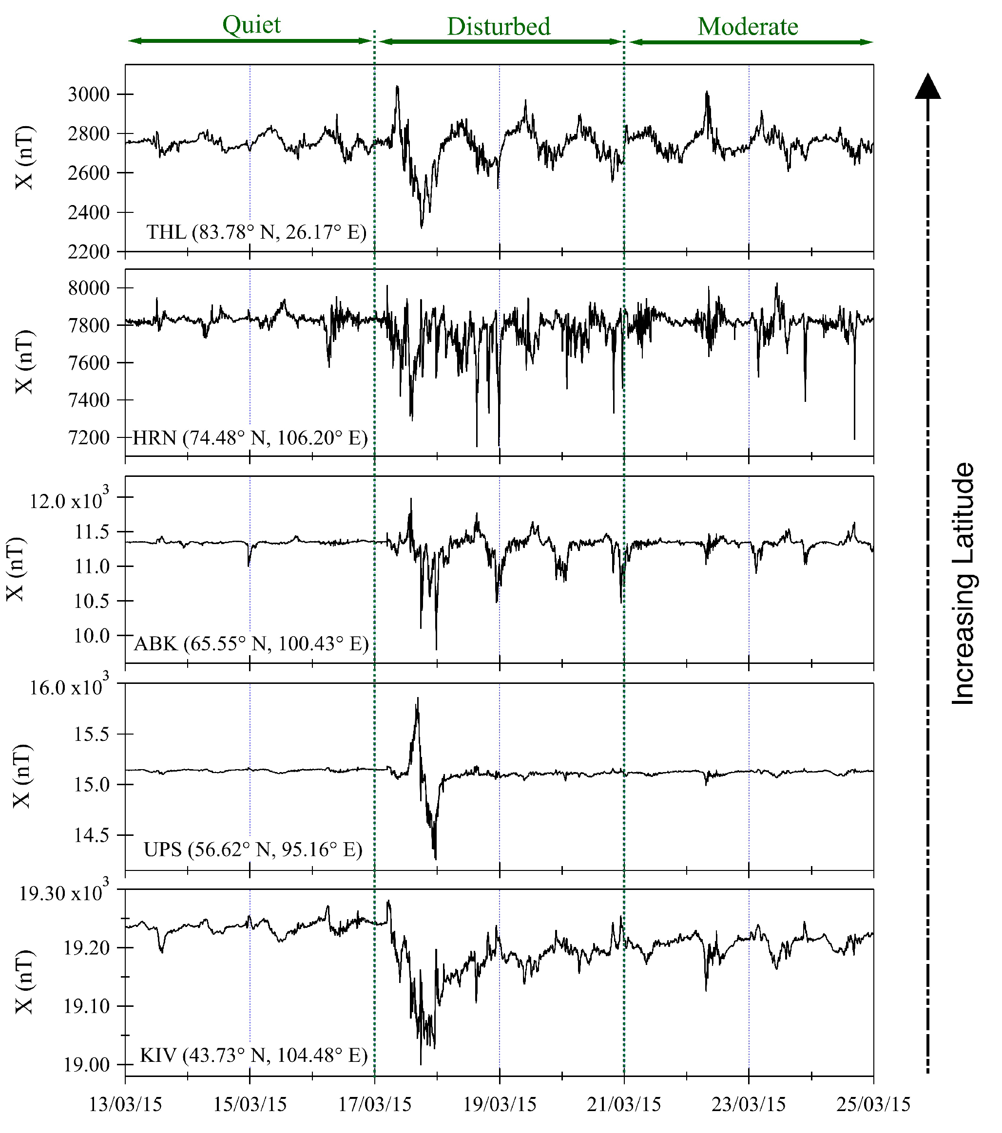
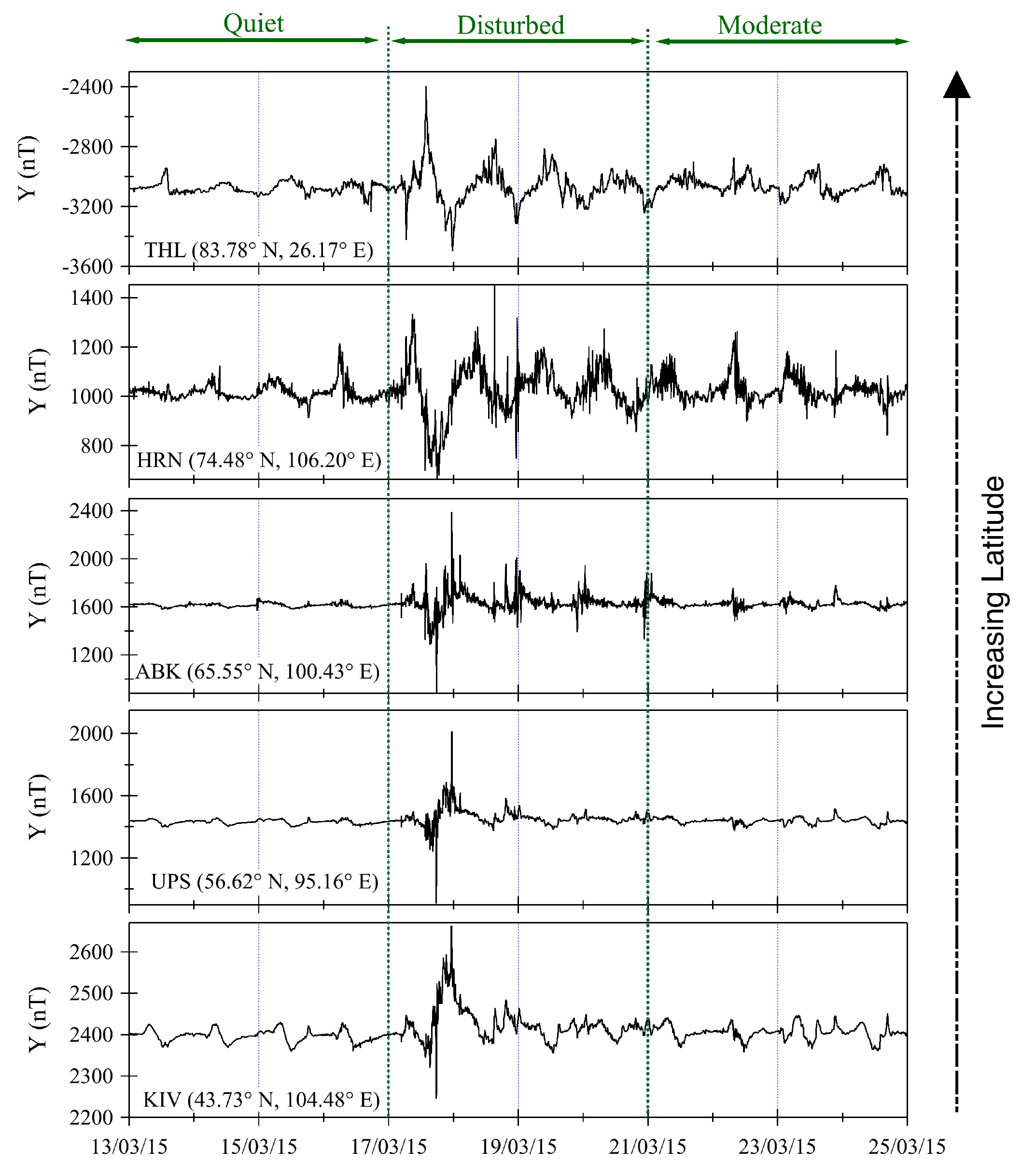
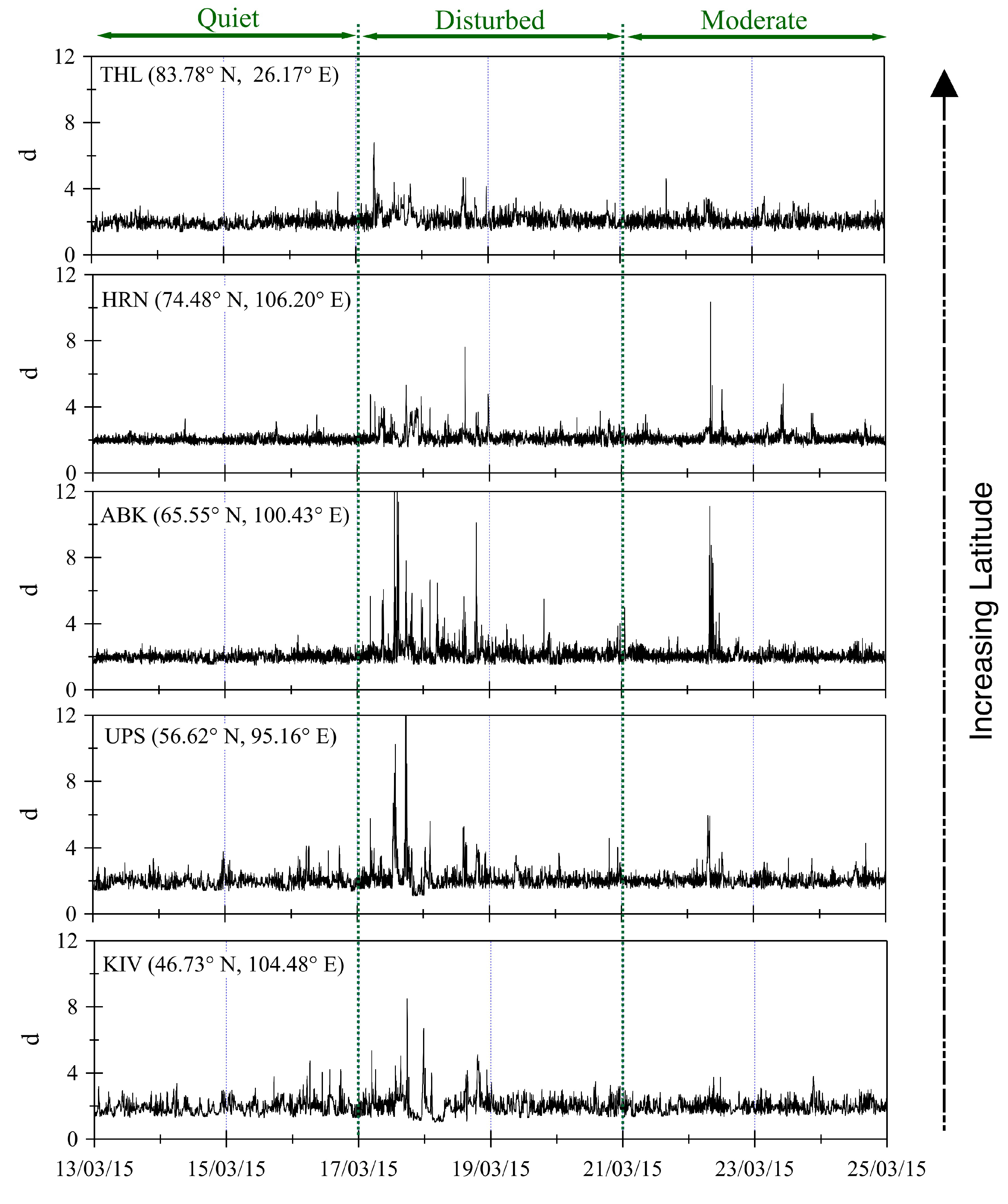
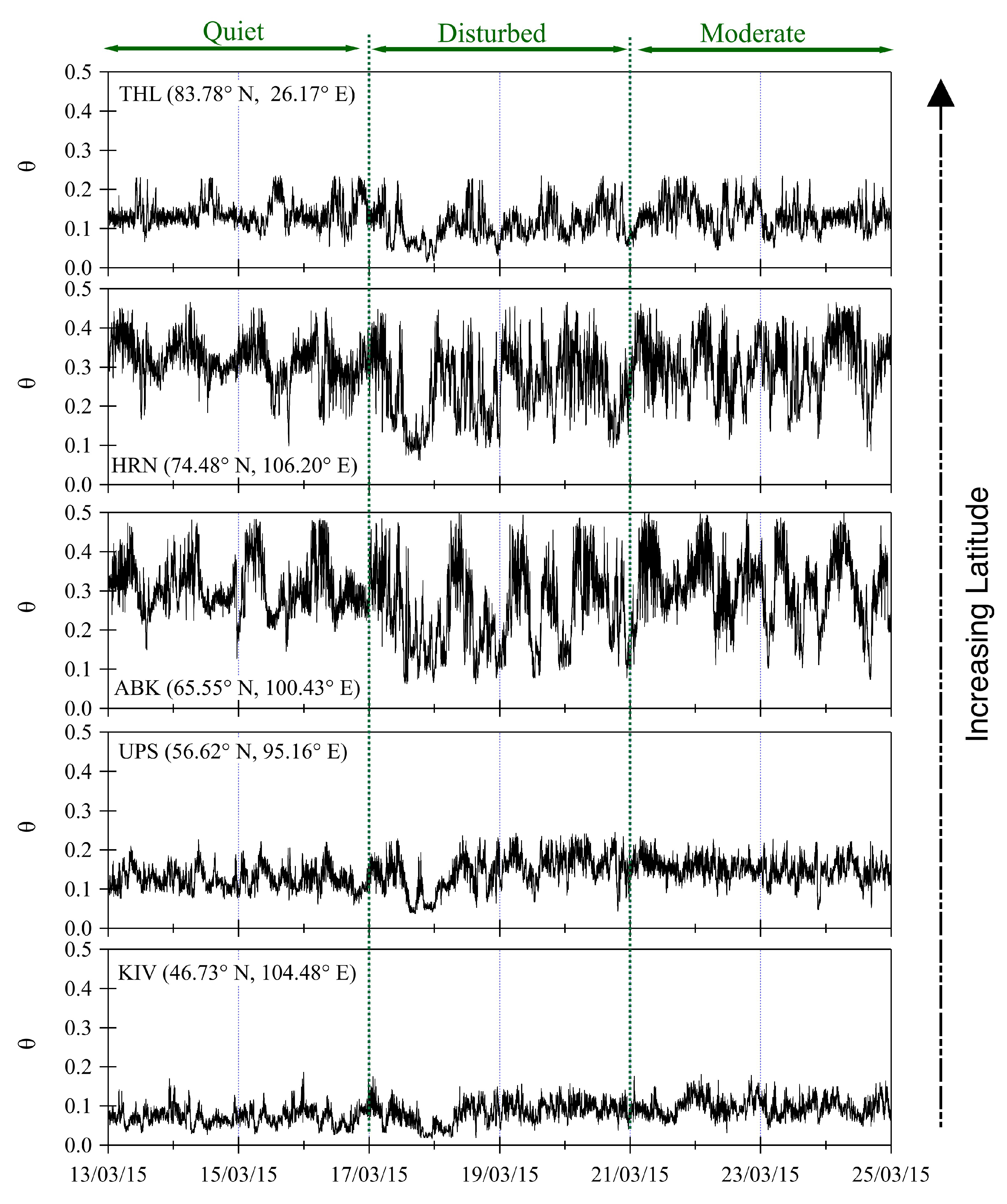
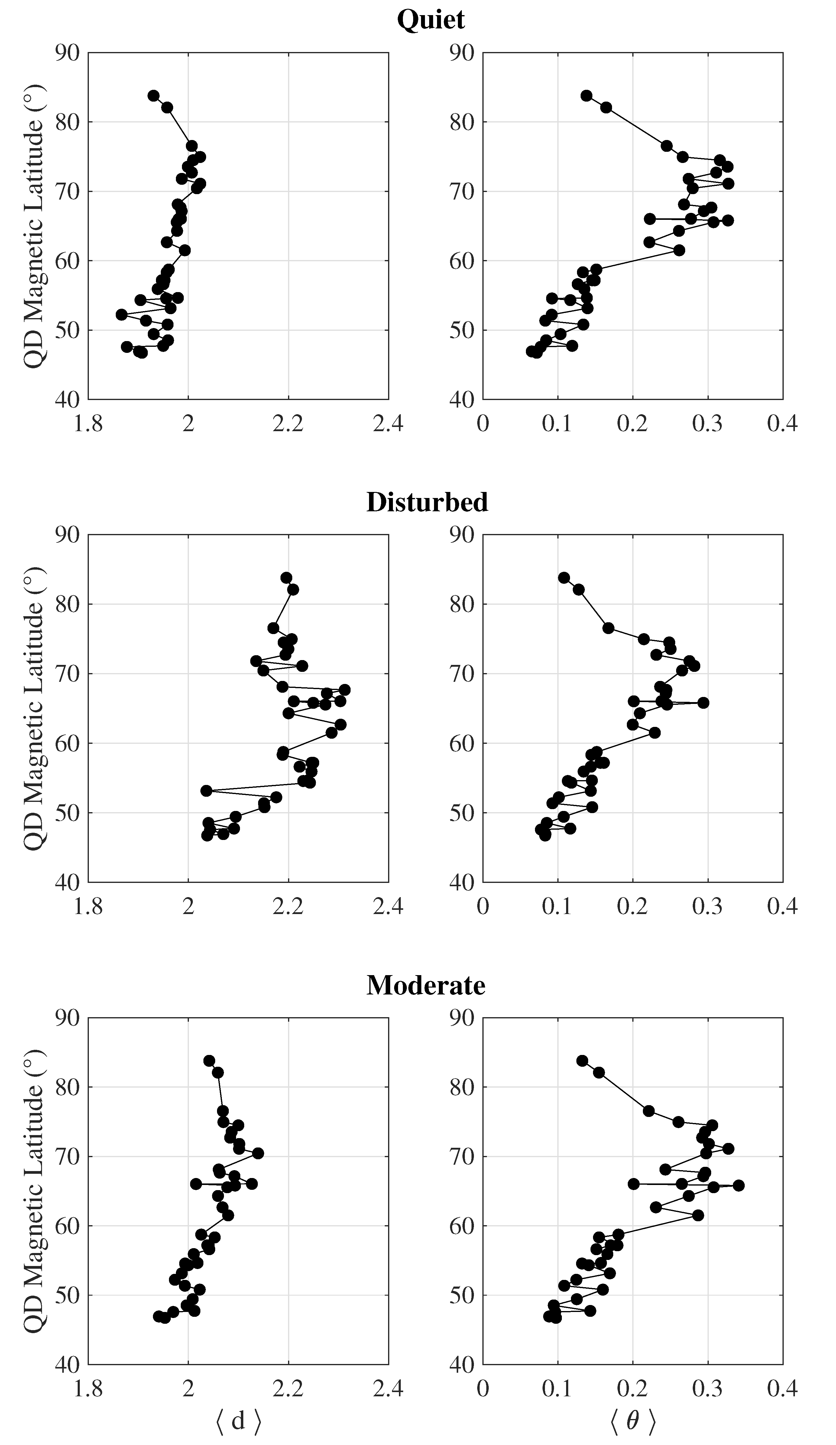
• The dynamics of the auroral oval are, instead, less persistent than higher/lower latitudes. This is one of the main novelties of our analysis. On average, our results are in agreement with Vassiliadis et al. [55] and Consolini [56], who reported an increase in the predictability power (at large scales, say >200 min) of the system during a disturbed period with respect to a quiet one, as a result of the strong driver imposed by the solar wind to the geomagnetic response, at both high and mid latitudes. Furthermore, Consolini [56], by using the Kolmogorov entropy which is related to the maximum temporal horizon for which a reliable prediction of a system can be done, also reported a dramatic decrease down to 2 min of the short-term variability (<200 min) of the magnetosphere–ionosphere system during a geomagnetic storm. Here, by using the inverse persistence $\theta$ we show how the predictability is a matter of latitudes and not only of scales [14,56], while the average dimensions are nearly independent of geomagnetic latitude. Indeed, the lowest values are found at lower latitudes, while the highest ones are observed across the auroral oval’s boundary (60$°$–70$°$N), with the latter slightly decreasing during the geomagnetic storm as a result of more persistent conditions caused by the external forcing from the solar wind acting as a driver of geomagnetic fluctuations [14].
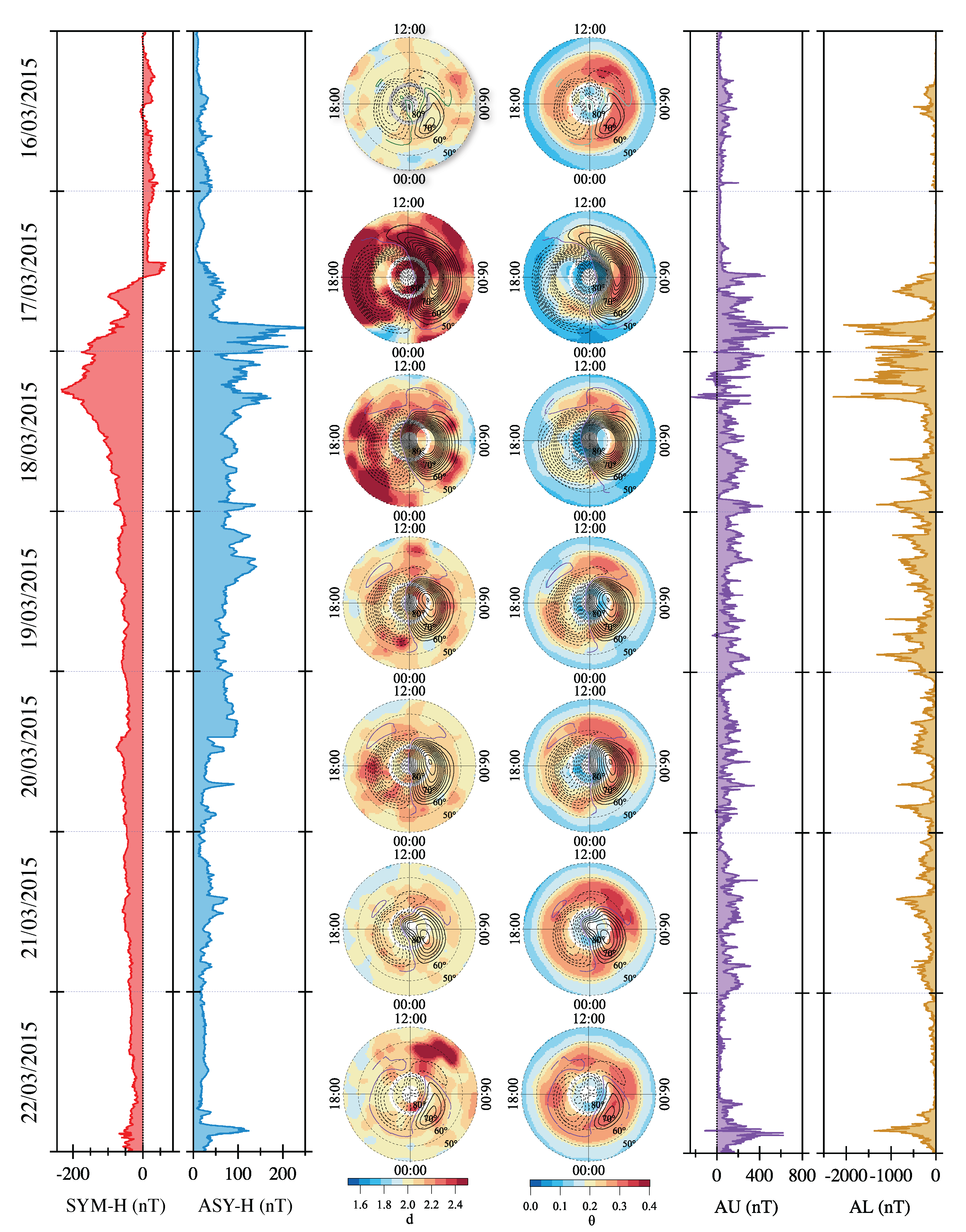
• By analyzing the daily polar-map behavior during a disturbed period, we show that higher values of the dimension are observed on days characterized by the initial phase of a magnetic storm and when a series of substorms is present. This increase in the value of the instantaneous dimension is due to the formation of an intense ring current and auroral currents affecting the magnetic field at low and high latitudes. We also show that the maximum values of the instantaneous dimension appear to be influenced by the evolution of the plasma convection cells, indicating a possible correlation with the presence and intensity of auroral electrojet currents. Regarding the daily trend of the inverse persistence $\theta$, there are always three distinct zones: one for latitudes greater than 80$°$, one with latitude values between 60$°$ and 80$°$ and one with latitude values less than 60$°$. The intermediate zone, i.e., the auroral oval boundary, is the one where the $\theta$ index takes higher values compared to the other two zones. This structure is clear on days of low or moderate activity.

Our results clearly framed out the magnetosphere–ionosphere system as a latitudinal-dependent ergodic low-dimensional system during quiet periods and a latitudinal-dependent deterministically driven high-dimensional system during a geomagnetic storm. This means that it cannot be reduced into smaller components and that its predictability is a matter of temporal (as in [14,56]) and spatial (i.e., latitudinal) scales. This study contributes to advancing our understanding of the complex dynamics of the Earth’s magnetosphere–ionosphere system and its response to external drivers, suggesting that the pair $(d,\theta )$ seems to be a promising tool for investigating the geomagnetic activity, both during quiet and disturbed periods and for discerning the role of high- vs. mid-latitude processes in terms of active degrees of freedom and persistent properties.

References

1. Merrill, R.T.; McElhinny, M.W.; McFadden, P.L.; Banerjee, S.K. The Magnetic Field of the Earth: Paleomagnetism, the Core and the Deep Mantle. Phys. Today 1997, 50, 70. [Google Scholar] [CrossRef]
2. Campbell, W.H. Introduction to Geomagnetic Fields, 2nd ed.; Wiley: Hoboken, NJ, USA, 2003. [Google Scholar]
3. Kamide, Y. Geomagnetic Storms as a Dominant Component of Space Weather: Classic Picture and Recent Issues. In Space Storms and Space Weather Hazards; Daglis, I.A., Ed.; Springer: Dordrecht, The Netherlands, 2001; pp. 43–77. [Google Scholar] [CrossRef]
4. Daglis, I.A. Space Storms, Ring Current and Space-Atmosphere Coupling. In Space Storms and Space Weather Hazards; Daglis, I.A., Ed.; Springer: Dordrecht, The Netherlands, 2001; pp. 1–42. [Google Scholar] [CrossRef]
5. Jordanova, V.K.; Ilie, R.; Chen, M. Ring Current Investigations. The Quest for Space Weather Prediction; Elsevier: Amsterdam, The Netherlands, 2020. [Google Scholar]
6. Sugiura, M. Hourly Values of equatorial Dst for the IGY. Ann. Int. Geophys. Yr. 1964, 35, 1–41. [Google Scholar]
7. Turner, N.E.; Baker, D.N.; Pulkkinen, T.I.; McPherron, R.L. Evaluation of the tail current contribution to Dst. J. Geophys. Res. 2000, 105, 5431–5440. [Google Scholar] [CrossRef] [Green Version]
8. Ohtani, S.; Nosé, M.; Rostoker, G.; Singer, H.; Lui, A.T.Y.; Nakamura, M. Storm-substorm relationship: Contribution of the tail current to Dst. J. Geophys. Res. 2001, 106, 21199–21210. [Google Scholar] [CrossRef]
9. Siscoe, G.L.; McPherron, R.L.; Jordanova, V.K. Diminished contribution of ram pressure to Dst during magnetic storms. J. Geophys. Res. Space Phys. 2005, 110, A12227. [Google Scholar] [CrossRef]
10. Akasofu, S.I. A Review of Studies of Geomagnetic Storms and Auroral/Magnetospheric Substorms based on the Electric Current Approach. Front. Astron. Space Sci. 2021, 7, 100. [Google Scholar] [CrossRef]
11. Kamide, Y.; Rostoker, G. What Is the Physical Meaning of the AE Index? EOS Trans. 2004, 85, 188–192. [Google Scholar] [CrossRef]
12. Coster, A.Y.; Erickson, P.; Lanzerotti, L. Space Weather Effects and Applications; John Wiley & Sons: Hoboken, NJ, USA, 2021; Volume 5. [Google Scholar] [CrossRef]
13. Borovsky, J.E. Perspective: Is Our Understanding of Solar-Wind/Magnetosphere Coupling Satisfactory? Front. Astron. Space Sci. 2021, 8, 5. [Google Scholar] [CrossRef]
14. Alberti, T.; Consolini, G.; Lepreti, F.; Laurenza, M.; Vecchio, A.; Carbone, V. Timescale separation in the solar wind-magnetosphere coupling during St. Patrick’s Day storms in 2013 and 2015. J. Geophys. Res. Space Phys. 2017, 122, 4266–4283. [Google Scholar] [CrossRef] [Green Version]
15. Alberti, T.; Consolini, G.; De Michelis, P.; Laurenza, M.; Marcucci, M.F. On fast and slow Earth’s magnetospheric dynamics during geomagnetic storms: A stochastic Langevin approach. J. Space Weather. Space Clim. 2018, 8, A56. [Google Scholar] [CrossRef] [Green Version]
16. Alberti, T.; Faranda, D.; Consolini, G.; De Michelis, P.; Donner, R.V.; Carbone, V. Concurrent Effects between Geomagnetic Storms and Magnetospheric Substorms. Universe 2022, 8, 226. [Google Scholar] [CrossRef]
17. Borovsky, J.E.; Valdivia, J.A. The Earth’s Magnetosphere: A Systems Science Overview and Assessment. Surv. Geophys. 2018, 39, 817–859. [Google Scholar] [CrossRef] [Green Version]
18. Chandorkar, M.; Camporeale, E. Chapter 9—Probabilistic Forecasting of Geomagnetic Indices Using Gaussian Process Models. In Machine Learning Techniques for Space Weather; Camporeale, E., Wing, S., Johnson, J.R., Eds.; Elsevier: Amsterdam, The Netherlands, 2018; pp. 237–258. [Google Scholar] [CrossRef]
19. Temmer, M. Space weather: The solar perspective. Living Rev. Sol. Phys. 2021, 18, 4. [Google Scholar] [CrossRef]
20. Foullon, C.; Malandraki, O. (Eds.) IAU Symposium Proceedings—Space Weather of the Heliosphere: Processes and Forecasts; Cambridge University Press: Cambridge, UK, 2018; Volume 335. [Google Scholar] [CrossRef] [Green Version]
21. Consolini, G.; Chang, T.; Lui, A.T. Complexity and topological disorder in the Earth’s magnetotail dynamics. In Nonequilibrium Phenomena in Plasmas; Springer: Berlin/Heidelberg, Germany, 2005; pp. 51–69. [Google Scholar] [CrossRef]
22. Iyemori, T. Storm-time magnetospheric currents inferred from mid-latitude geomagnetic field variations. J. Geomagn. Geoelectr. 1990, 42, 1249–1265. [Google Scholar] [CrossRef]
23. Davis, T.N.; Sugiura, M. Auroral electrojet activity index AE and its universal time variations. J. Geophys. Res. 1966, 71, 785–801. [Google Scholar] [CrossRef] [Green Version]
24. Wanliss, J.A.; Showalter, K.M. High-resolution global storm index: Dst versus SYM-H. J. Geophys. Res. Space Phys. 2006, 111, A02202. [Google Scholar] [CrossRef]
25. Wanliss, J. Fractal properties of SYM-H during quiet and active times. J. Geophys. Res. Space Phys. 2005, 110, A03202. [Google Scholar] [CrossRef]
26. Richmond, A.D. Ionospheric electrodynamics using magnetic apex coordinates. J. Geomagn. Geoelectr. 1995, 47, 191–212. [Google Scholar] [CrossRef]
27. Gjerloev, J.W. The SuperMAG data processing technique. J. Geophys. Res. Space Phys. 2012, 117, A09213. [Google Scholar] [CrossRef]
28. Lucarini, V.; Faranda, D.; Wouters, J.; Kuna, T. Towards a General Theory of Extremes for Observables of Chaotic Dynamical Systems. J. Stat. Phys. 2014, 154, 723–750. [Google Scholar] [CrossRef]
29. Moreira Freitas, A.C.; Milhazes Freitas, J.; Todd, M. Extremal Index, Hitting Time Statistics and periodicity. arXiv 2010, arxiv:1008.1350. [Google Scholar]
30. Lucarini, V.; Faranda, D.; Wouters, J. Universal Behaviour of Extreme Value Statistics for Selected Observables of Dynamical Systems. J. Stat. Phys. 2012, 147, 63–73. [Google Scholar] [CrossRef] [Green Version]
31. Lucarini, V.; Faranda, D.; de Freitas, A.C.G.M.M.; de Freitas, J.M.M.; Holland, M.; Kuna, T.; Nicol, M.; Todd, M.; Vaienti, S. Extremes and Recurrence in Dynamical Systems; Wiley: New York, NY, USA, 2016. [Google Scholar]
32. Grassberger, P.; Procaccia, I. Characterization of strange attractors. Phys. Rev. Lett. 1983, 50, 346–349. [Google Scholar] [CrossRef]
33. Grassberger, P.; Procaccia, I. Measuring the strangeness of strange attractors. Phys. D Nonlinear Phenom. 1983, 9, 189–208. [Google Scholar] [CrossRef]
34. Hentschel, H.G.E.; Procaccia, I. The infinite number of generalized dimensions of fractals and strange attractors. Phys. D Nonlinear Phenom. 1983, 8, 435–444. [Google Scholar] [CrossRef]
35. Moloney, N.R.; Faranda, D.; Sato, Y. An overview of the extremal index. Chaos 2019, 29, 022101. [Google Scholar] [CrossRef] [PubMed] [Green Version]
36. Süveges, M. Likelihood estimation of the Extremal index. Extremes 2007, 10, 41–55. [Google Scholar] [CrossRef]
37. Faranda, D.; Alvarez-Castro, M.C.; Messori, G.; Rodrigues, D.; Yiou, P. The hammam effect or how a warm ocean enhances large scale atmospheric predictability. Nat. Commun. 2019, 10, 1316. [Google Scholar] [CrossRef] [PubMed] [Green Version]
38. De Luca, P.; Messori, G.; Faranda, D.; Ward, P.J.; Coumou, D. Compound warm–dry and cold–wet events over the Mediterranean. Earth Syst. Dyn. 2020, 11, 793–805. [Google Scholar] [CrossRef]
39. Faranda, D.; Vrac, M.; Yiou, P.; Jézéquel, A.; Thao, S. Changes in future synoptic circulation patterns: Consequences for extreme event attribution. Geophys. Res. Lett. 2020, 47, e2020GL088002. [Google Scholar] [CrossRef]
40. Faranda, D.; Messori, G.; Yiou, P. Diagnosing concurrent drivers of weather extremes: Application to warm and cold days in North America. Clim. Dyn. 2020, 54, 2187–2201. [Google Scholar] [CrossRef]
41. Giamalaki, K.; Beaulieu, C.; Faranda, D.; Henson, S.; Josey, S.; Martin, A. Signatures of the 1976–1977 regime shift in the north pacific revealed by statistical analysis. J. Geophys. Res. Ocean. 2018, 123, 4388–4397. [Google Scholar] [CrossRef]
42. Alberti, T.; Daviaud, F.; Donner, R.V.; Dubrulle, B.; Faranda, D.; Lucarini, V. Chameleon attractors in turbulent flows. Chaos Solitons Fract. 2023, 168, 113195. [Google Scholar] [CrossRef]
43. Alberti, T.; Faranda, D.; Donner, R.V.; Caby, T.; Carbone, V.; Consolini, G.; Dubrulle, B.; Vaienti, S. Small-scale Induced Large-scale Transitions in Solar Wind Magnetic Field. Astrophys. J. Lett. 2021, 914, L6. [Google Scholar] [CrossRef]
44. Gualandi, A.; Avouac, J.P.; Michel, S.; Faranda, D. The predictable chaos of slow earthquakes. Sci. Adv. 2020, 6, eaaz5548. [Google Scholar] [CrossRef]
45. Gualandi, A.; Faranda, D.; Marone, C.; Cocco, M.; Mengaldo, G. Deterministic and stochastic chaos characterize laboratory earthquakes. Earth Planet. Sci. Lett. 2023, 604, 117995. [Google Scholar] [CrossRef]
46. Gonzalez, W.D.; Clúa de Gonzalez, A.L.; Tsurutani, B.T. Geomagnetic response to large-amplitude interplanetary Alfvén wave trains. Phys. Scr. Vol. T 1994, 55, 140. [Google Scholar] [CrossRef]
47. Tsurutani, B.T.; Sugiura, M.; Iyemori, T.; Goldstein, B.E.; Gonzalez, W.D.; Akasofu, S.I.; Smith, E.J. The nonlinear response of AE to the IMF BS driver: A spectral break at 5 h. Geophys. Res. Lett. 1990, 17, 279–282. [Google Scholar] [CrossRef] [Green Version]
48. Akasofu, S.I. Auroral Substorms: Search for Processes Causing the Expansion Phase in Terms of the Electric Current Approach. Space Sci. Rev. 2017, 212, 341–381. [Google Scholar] [CrossRef] [Green Version]
49. De Michelis, P.; Consolini, G.; Materassi, M.; Tozzi, R. An information theory approach to the storm-substorm relationship. J. Geophys. Res. Space Phys. 2011, 116, A08225. [Google Scholar] [CrossRef]
50. De Michelis, P.; Tozzi, R.; Consolini, G. Principal components’ features of mid-latitude geomagnetic daily variation. Ann. Geophys. 2010, 28, 2213–2226. [Google Scholar] [CrossRef] [Green Version]
51. Alberti, T.; Piersanti, M.; Vecchio, A.; De Michelis, P.; Lepreti, F.; Carbone, V.; Primavera, L. Identification of the different magnetic field contributions during a geomagnetic storm in magnetospheric and ground observations. Ann. Geophys. 2016, 34, 1069–1084. [Google Scholar] [CrossRef] [Green Version]
52. Carlson, H.C., Jr. Dynamics of the quiet polar cap. J. Geomagn. Geoelectr. 1990, 42, 697–710. [Google Scholar] [CrossRef]
53. Emmert, J.T.; Richmond, A.D.; Drob, D.P. A computationally compact representation of Magnetic-Apex and Quasi-Dipole coordinates with smooth base vectors. J. Geophys. Res. Space Phys. 2010, 115, A08322. [Google Scholar] [CrossRef] [Green Version]
54. Cousins, E.D.P.; Shepherd, S.G. A dynamical model of high-latitude convection derived from SuperDARN plasma drift measurements. J. Geophys. Res. Space Phys. 2010, 115, A12329. [Google Scholar] [CrossRef]
55. Vassiliadis, D.V.; Sharma, A.S.; Eastman, T.E.; Papadopoulos, K. Low-dimensional chaos in magnetospheric activity from AE time series. Geophys. Res. Lett. 1990, 17, 1841–1844. [Google Scholar] [CrossRef] [Green Version]
56. Consolini, G. Chapter 7—Emergence of Dynamical Complexity in the Earth’s Magnetosphere. In Machine Learning Techniques for Space Weather; Camporeale, E., Wing, S., Johnson, J.R., Eds.; Elsevier: Amsterdam, The Netherlands, 2018; pp. 177–202. [Google Scholar] [CrossRef]
Figure 1. Temporal trend of AL, AU, SYM-H and ASY-H from 13 March to 24 March 2015. The green vertical dotted lines identify three periods with varying levels of geomagnetic activity: quiet, disturbed and moderate.
Remotesensing 15 03031 g001
Figure 2. The geographical distribution of the selected geomagnetic stations and observatories.
Remotesensing 15 03031 g002
Figure 3. The X component of the geomagnetic field measured at five different observatories between 13 and 24 March 2015, located at different magnetic latitudes (increasing from bottom to top). The green dotted lines demarcate time intervals distinguished by different levels of geomagnetic activity.
Remotesensing 15 03031 g003
Figure 4. The Y component of the geomagnetic field measured at five different observatories between 13 and 24 March 2015, located at different magnetic latitudes (increasing from bottom to top). The green dotted lines demarcate time intervals distinguished by different levels of geomagnetic activity.
Remotesensing 15 03031 g004
Figure 5. The instantaneous dimensions d evaluated at five different observatories between 13 and 24 March 2015. The green dotted lines demarcate time intervals distinguished by different levels of geomagnetic activity.
Remotesensing 15 03031 g005
Figure 6. The inverse persistence θ evaluated at five different observatories between 13 and 24 March 2015. The green dotted lines demarcate time intervals distinguished by different levels of geomagnetic activity.
Remotesensing 15 03031 g006
Figure 7. The average dimension d (left panels) and the average inverse persistence θ (right panels) as a function of the geomagnetic latitude λ during the quiet (top), the disturbed (middle) and the moderate (bottom) periods of geomagnetic activity.
Remotesensing 15 03031 g007
Figure 8. SYM-H and ASY-H indices are shown on the left. In the middle: Daily polar view maps of the Northern Hemisphere’s instantaneous dimensions d and inverse persistence θ . The information is presented in magnetic latitude (50 ° to 90 ° ) and magnetic local time (MLT) coordinate systems, with concentric circles representing magnetic latitude contours separated by 10 ° intervals. The SuperDARN polar potential maps obtained using the statistical convection model CS10 are superimposed on magnetic field maps. The maps cover the week of 16 March to 22 March 2015. The AU and AL indices are shown on the right.
Remotesensing 15 03031 g008