


Use of Landsat Satellite Images in the Assessment of the Variability in Ice Cover on Polish Lakes


1
Department of Land Improvement, Environmental Development and Spatial Management, Poznań University of Life Sciences, Piątkowska 94E, 60-649 Poznań, Poland
2
Department of Hydrology and Water Management, Adam Mickiewicz University, B. Krygowskiego 10, 61-680 Poznań, Poland
3
College of Hydraulic Science and Engineering, Yangzhou University, Yangzhou 225009, China
*
Author to whom correspondence should be addressed.
Remote Sens. 2023, 15(12), 3030; https://doi.org/10.3390/rs15123030
Submission received: 29 April 2023
/
Revised: 2 June 2023
/
Accepted: 8 June 2023
/
Published: 9 June 2023
(This article belongs to the Special Issue Remote Sensing of Environmental Changes in Cold Regions Ⅱ)
Abstract
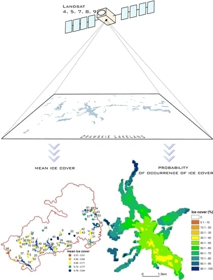
:Despite several decades of observations of ice cover in Polish lakes, researchers have not broadly applied satellite images to date. This paper presents a temporal and spatial analysis of the variability in the occurrence of ice cover on lakes in the Drawskie Lakeland in the hydrological years 1984–2022 based on satellite data from Landsat missions 4, 5, 7, 8, and 9. The range of occurrence of ice cover was determined based on the value of the Normalised Difference Snow Index (NDSI) and blue spectral band (). The determination of ice cover extent adopted values from 0.033 to 0.120 as the threshold values. The analysis covered 67 lakes with an area from 0.07 to 18.71 km2. A total of 53 images were analysed, 14 and 39 out of which showed full and partial ice cover, respectively. The cluster analysis permitted the designation of two groups of lakes characterised by an approximate range of ice cover. The obtained results were analysed in the context of the morphometric parameters of the lakes. It was evidenced that the range of the ice cover on lakes is determined by the surface area of the lakes; their mean and maximum depth, volume, length, and width; and the height of the location above sea level. The results of analyses of the spatial range of ice cover in subsequent scenes allowed for the preparation of maps of probability of ice cover occurrence that permit the complete determination of its variability within each of the lakes. Monitoring of the spatial variability in ice cover within individual lakes as well as in reference to lakes not subject to traditional observations offers new research possibilities in many scientific disciplines focused on these ecosystems.
1. Introduction
Elements of the hydrosphere of moderate latitudes undergo seasonal changes determined by climatic conditions. Parameters of rivers and lakes change broadly from high water temperatures in the summer season to a change in the physical state in the winter season, where the appearance of ice cover completely changes their functioning in comparison to other seasons. Due to this, the issue of ice cover is a frequently discussed subject that refers to both the physicochemical and biological conditions. Ice cover shapes the distribution of dissolved oxygen [1,2], light dispersion [3,4], metabolic dynamics [5], and heat content [6]. Research conducted on Lake Ulansuhai (China) showed that the presence of ice in the winter season may cause a rapid increase in nutrient concentration in water and sediments [7]. Moreover, a decline in ice cover favours wave growth in winter, as evidenced by the analysis of Lake Michigan [8]. The presence of ice affects the composition and activity of plankton [9,10] and waterfowl [11].
In the case of Poland, more than 7000 natural lakes exist across the country [12], constituting an important element of the natural environment, particularly in the north of Poland where they are the most abundant [13]. Numerous analyses of ice cover on lakes have been conducted to date [14,15,16,17,18,19], but the information is still limited to a relatively small population (several tens of lakes) under systematic monitoring. They are lakes with surface areas from 100 to 11,000 ha. They are therefore relatively large for Poland, where the average surface area of all lakes is 39.6 ha. [12]. This background lacks a reference to information on the remaining lakes, those with a smaller surface area that are equally important in environmental and economic terms. Importantly, study results for 220 lakes in the northern hemisphere showed that despite common warming patterns, individual lake parameters may determine the rate of loss of ice cover, and this knowledge is necessary for future activities in the scope of environmental modelling and protection [20]. Expanding knowledge in the scope of ice cover on lakes is possible owing to the application of remote sensing methods that have been dynamically developing at least for the last several decades.
Technical progress supports an increase in the accuracy and possibilities of satellite methods as well as the use of various combinations of data. Heinilä et al. [21] applied the method of accessing data regarding ice cover range in lakes based on multidimensional Gaussian distributions calculated for training data with the application of several reflectance and thermal bands and related indices. In the case of large lakes in the northern hemisphere, Wu et al. [22] assessed the ability of four machine learning classifiers to map ice cover of lakes, water, and cloudiness during periods of ice disintegration and freezing. It was determined that all classifiers using a combination of seven bands proved able to generate total classification accuracy above 94%. Wang et al. [23] investigated the efficiency of the semiautomatic segmentation “glocal” Iterative Region Growing with Semantics (IRGS) algorithm for the classification of lake ice by means of dual polarity RADARSAT-2 images obtained over Lake Erie. The analysis of Lake Erie showed that the “glocal” IRGS algorithm can provide credible ice–water classification by means of dually polarised images featuring high total accuracy.
Satellite images permitted monitoring surface water/ice dynamics both in space and in time, although using them involves many challenges [24]. According to Herrick et al. [25] in the case of teledetection data, the dataset is still mainly available to experts in the field, and requires advanced skills. The method proposed herein applies a relatively simple approach illustrating the so-far-unavailable information regarding ice cover in Poland, based on remote sensing data. This offers new possibilities of investigation of lake ecosystems in reference to the phases of appearance and disappearance of ice, zones of its presence, and probability of occurrence. This information is key for fields such as limnology, hydrobiology, and ecology.
The study objective is the determination of the variability in occurrence of ice cover on selected lakes in Poland, and the determination of the effect of selected morphometric parameters on the occurrence of ice.
2. Materials and Methods
2.1. Study Area
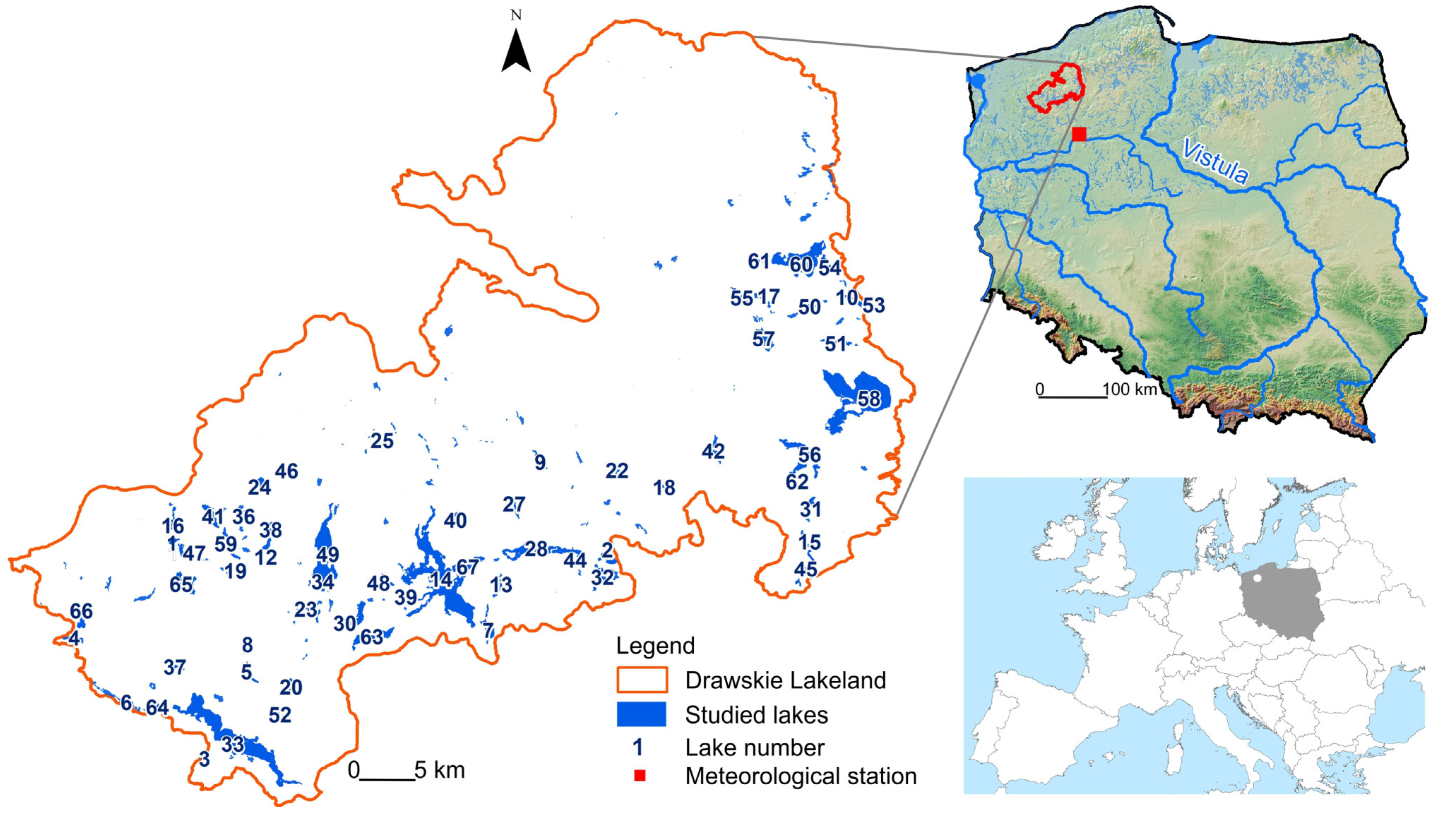
The study area covered the Drawskie Lakeland in the northwestern part of Poland. The area features deep postglacial channels containing numerous lakes. The Drawskie Lakeland is enormously rich in terms of occurrence of lakes and other small water bodies. It includes approximately 500 of them (with a surface area of more than 1 ha). For 67 lakes, it was possible to determine detailed morphometric parameters, including: volume, maximum and mean depth, length, effective length, width, shoreline length and development, and exposure index (Figure 1; Table S1) [26]. These lakes served as a further subject of the analysis of occurrence of ice cover. The largest lakes in the study area are Drawsko (18.1 km2), Wielimie (16.9 km2), Lubie (14.4 km2), Siecino (7.2 km2), Wierzchowo (7.0 km2), and Komorze (3.9 km2). The largest rivers in the Drawskie Lakeland include Drawa, Gwda, Parsęta, and Rega. Together with their smaller tributaries, they constitute a well-developed hydrographic system.
2.2. Materials
This study used the USGS Earth Resources Observation and Science (EROS) Archive—Landsat Archives dataset: Landsat 4–5 TM, Landsat 7 ETM+, Landsat 8 OLI, and Landsat 9OLI + Collection 2 Level-1 Tier 1 and Tier 2. The compiled dataset refers to the cool half-year (November–April) and covers the period 1984–2022. The Drawskie Lakeland is located on path 191 and 192 on the interface of lines 22 and 23. The preliminary analysis covered scenes with cloud covers of up to 70%. Then, each scene was analysed in detail in terms of occurrence of cloud cover within the studied lakes. For the purpose of the identification of clouds and cloud shade, the CFMask algorithm [27] was applied. It was assumed that if no cloud cover occurred within the range of Lakes Lubie, Drawsko, Siecino, and Wielimie (the largest of the analysed lakes), the scene was qualified for further research procedures. As a result, a total of 181 Landsat scenes were selected for the analysis, including 152 scenes for Tier 1 and 29 for Tier 2 products. Each Landsat scene involves processing to one of the three levels: L1TP (Precision and Terrain Correction), L1GT (Systematic Terrain Correction), or L1GS (Systematic Correction) (https://www.usgs.gov/landsat-missions/landsat-levels-processing, accessed on 10 March 2023). Furthermore, Landsat 7 scenes had data missing as of June 2003 due to a failure of the Scan Line Corrector (SLC). The strip lines were gap-filled using Landsat toolbox’s ‘fix Landsat 7 scan line error’ of ArcGIS software [28]. This study used 160 scenes processed to L1TP, and 21 scenes processed to L1GS.
This study also used the morphometric parameters of the lakes presented in the Atlas of Polish Lakes, which are: volume, maximum depth, mean depth, length, effective length, width, shoreline length, shoreline development, and exposure index. The data for individual lakes are presented in Table S1.
2.3. Methods
At the first stage, for all available scenes, top of atmosphere (TOA) reflectance ρλ was calculated using the following equations [29]:
where:
- —TOA planetary spectral reflectance, without correction for solar angle (-);
- —reflectance multiplicative scaling factor for the band (-);
- —level 1 pixel value in DN (-);
- —reflectance additive scaling factor for the band.
The values of and were obtained from the metadata (MTL.txt) file distributed with the Landsat Collection 2 Level-1 data products. The ρλ’ value is not the real TOA reflectance, because it does not contain a correction for the solar elevation angle. Therefore, in the second step, the solar elevation angle was taken into account, and the real TOA reflectance ρλ was calculated using the following equation:
where:
- —real TOA planetary reflectance (-);
- —local solar zenith angle.
The purpose of calculating the real TOA reflectance is to standardise the input data for the subsequent stages of the analysis. Hence, the albedo range is usually between 0 and 1, which is unitless and represents the ratio of solar radiation that is reflected [30].
This procedure completed the preparation of data of the L1TP level. Data from the L1GS level required additional assigning of georeference due to the fact that the available scenes were not shifted in reference to the actual location. For this purpose, 1st-order polynomial transformation available in ArcGIS Pro software [ESRI, Inc., Redlands, CA, USA] was used. Each of the 181 available scenes was subject to the analysis of ice cover on lakes. This permitted assigning one of three classes to each scene: 0—no ice cover on any of the lakes; 1—partial ice cover, 2—full ice cover on all lakes.
The starting point of identification of the lakes’ spatial extent was the 2022 Hydrographic Division Map of Poland at a scale of 1:10,000, made available by the National Water Holding Polish Waters (Państwowe Gospodarstwo Wodne—Wody Polskie). The data were accessed through Hydroportal (https://wody.isok.gov.pl/imap_kzgw/?gpmap=gpSIGW, accessed on 6 February 2023). Because the analysis covers 38 years, the water surface area could have been changing throughout that period due to the development of water vegetation within the range of the littoral zone or short- or long-term water level fluctuations in the lakes due to climate change. In this regard, the spatial extent of the lakes was verified each time. This was conducted using the Normalised Difference Water Index (NDWI) calculated based on the following formula [31]:
where:
- —green spectral band;
- —near-infrared spectral band.
The NDWI values are within the range from −1 to 1, and for water objects, it adopts values higher than 0.2.
The next stage involved the detection of the occurrence of ice cover within the range of particular lakes in the Drawskie Lakeland. The analysis of the lake ice cover employed a method combining the Normalised Difference Snow Index (NDSI) and blue band proposed by Cáceres et al. [30]. The detection of ice cover was based on NDSI calculated based on the following formula [32]:
where:
- —green spectral band;
- —short-wave infrared spectral band.
NDSI can adopt values in a range from −1 to 1, whereas the probability of snow occurrence is proportional to how close the value is to 1. Moreover, the detection of occurrence of ice cover involved the application of TOA reflectance values for the blue band ρλ(blue). The following assumption was adopted at the stage of ice cover delimitation:
where:
- —blue spectral band;
- a, b—threshold values.
During the determination of the range of ice cover, an NDSI value of 0.4 (a) was adopted as the threshold value. The analysis of ice cover occurring within the analysed lakes showed that it was impossible to determine universal threshold values b for the entire analysed period, or even for a single full winter season. This is related to the occurrence of ice cover in different phases (1—phase of development of ice cover on lakes, 2—intermelting phase with periodically occurring water layer on top of ice cover, or phase of disintegration of ice cover) and co-occurrence of snow cover. Due to the above, the detailed analysis covered two test lakes with the most frequently occurring partial ice cover, namely, lakes Drawsko and Siecino. They were subject to manual mapping of water surface and ice cover. The resulting learning dataset permitted the determination of threshold values b—Lake Drawsko, and the validation dataset allowed for the verification of the previously adopted values—Lake Siecino. Based on Lake Drawsko, the values of were determined for the ice cover zone. The percentile 1% value was used as the threshold value. Subsequently, this value was used to determine the extent of ice cover in Lake Siecino. In subsequent steps, percentile values of 2 and 3% were tested. The analysis was completed when a consistency was obtained between the ice cover determined manually and that based on percentile thresholds of 98%. The threshold value of parameter b during subsequent analyses of ice cover was in a range from 0.033 to 0.120. The analysis resulted in a dataset with data gaps for smaller lakes due to cloud cover. The dataset was used to determine a relationship between ice cover in individual lakes (the analysis was performed for each lake). Finally, the missing data were supplemented with data from the lake for which the strongest relationship was obtained.
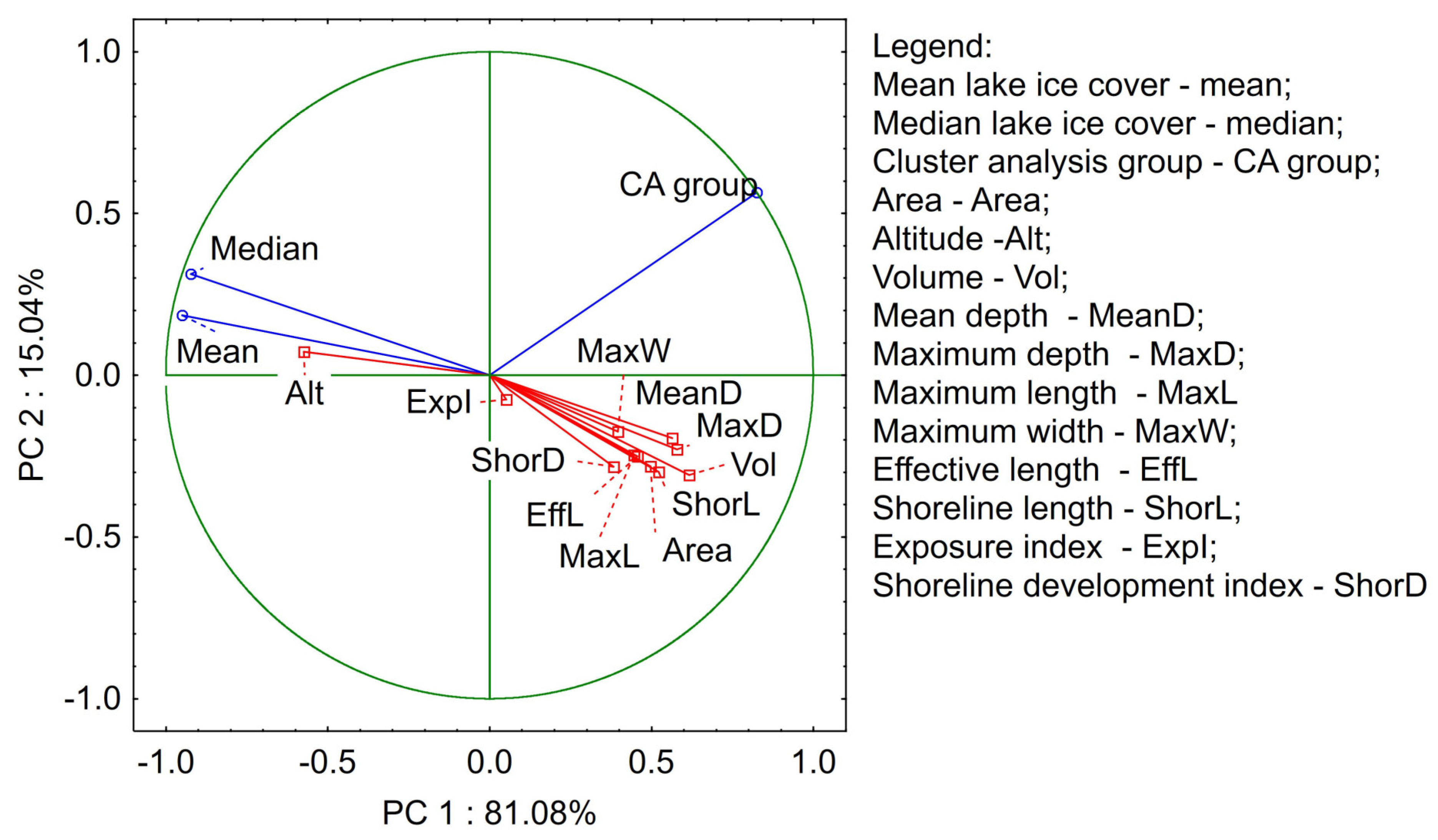
Grouping lakes by probability of occurrence of ice cover employed hierarchical cluster analysis (CA). The cluster analysis was conducted by means of the Ward method, adopting square Euclidean distance as the probability measure. The identification of factors determining the course of ice cover in selected groups of lakes involved the application of the principal component analysis (PCA). The PCA was conducted separately for each group of lakes, and for the entire dataset combined. The PCA analysis made it possible to investigate general patterns in the relationship between the presence of ice cover in lakes and the lakes’ morphometric parameters. The following morphometric lake parameters were considered: surface area (Area), altitude (Alt), maximum depth (MaxD), average depth (MeanD), volume (Vol), shoreline development (ShorD), exposure index (I), width (MaxW), length (MaxL), and effective length (EffL). The PCA analysis permits the presentation of data in new (orthogonal) spaces defined by principal components (PC). The number of PC was selected based on a Kaiser criterion of eigenvalues higher than 1. The relationship between PCs and analysed parameters was classified according to the values >0.75, 0.75–0.50, and 0.50–0.30 proposed by Liu et al. [33] as strong, moderate, and weak, respectively.
Finally, the degree of ice cover of lakes was analysed in reference to accumulated freezing degree days (AFDD) based on daily air temperature measurements for the Piła station (Figure 1). Freezing degree days (FDD) were calculated for each day from November to April as follows:
where:
FDD = (0 − Ta)
- Ta—average daily air temperature in degrees Celsius.
A negative FDD value represented a temperature warmer than freezing, while a positive FDD value represented a temperature below freezing. The FDD values for each day of winter were added together to determine the AFDD for each winter season. Values of the coefficient of correlation between ice cover on the lake on a specific date and the AFDD value was calculated. Due to the strong relationship between lake water temperatures and air temperature at the Pila meteorological station during the AFDD calculation, no lapse rate adjustment was used to adjust the temperature from the meteorological station elevation to the lakes’ elevations.
3. Results and Discussion
3.1. Temporary Changes in Lake Ice Cover
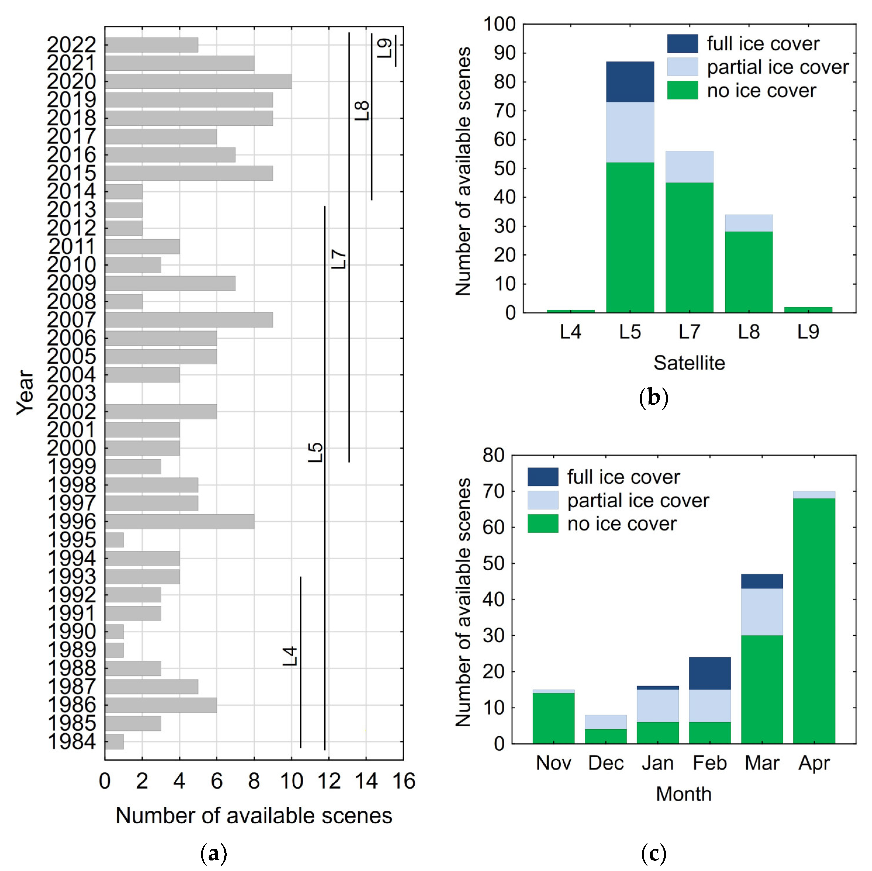
This section presents the research material for the analysis of ice cover on lakes of the Drawskie Lakeland, obtained for the period from November to April (winter half-year). In that period, due to the periodical occurrence of air temperatures below zero, ice cover occurred on the lakes, beginning with partial ice cover leading to full ice cover. The number of obtained images in particular periods and by subsequent satellites of the Landsat programme is presented in Figure 2a.
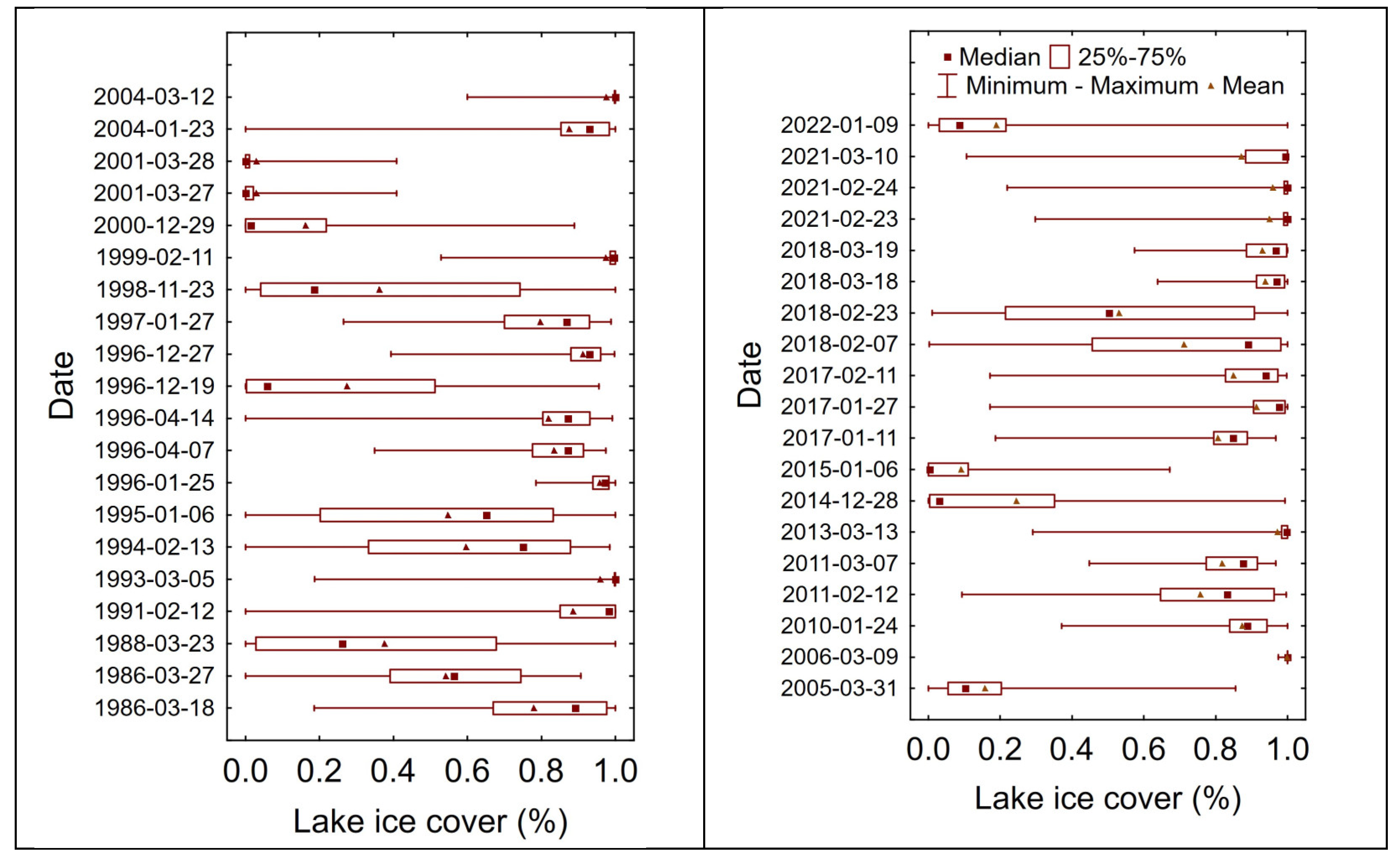
The highest number of scenes (10) was obtained in the hydrological winter half-year 2020, and no cloudless scene was obtained for the hydrological winter half-year 2003. The highest number of scenes for analysis was provided by satellite Landsat 5—87 scenes—and satellites Landsat 4 and Landsat 9 provided 1 and 2 scenes, respectively (Figure 2b). Only scenes from Landsat 5 documented full ice cover—defined as the occurrence of full ice cover on all the analysed lakes. Scenes from satellites Landsat 4 and Landsat 9 documented no occurrence of ice cover on any of the analysed lakes. The analysis of the collected data from particular months revealed that the highest number of scenes for analysis was available for April (70), and the lowest for December (8) (Figure 2c). In November, December, and April, full ice cover on all analysed lakes did not occur, and in January, February, and March, full ice cover on all lakes was documented in one, nine, and four images, respectively. Scenes from November, December, and April show no full ice cover on all analysed lakes. Scenes with partial ice cover on lakes are the most valuable from the point of view of the study. A total of 39 such scenes were obtained, 1 for November, 4 for December, 9 for January, 10 for February, 13 for March, and 2 for April. Results obtained from the analysis of these images were used for the assessment of the effect of lake morphometric parameters on the occurrence of ice cover. The occurrence of ice cover on particular lakes was determined as the ratio of ice cover surface area and water surface area on the lake. The range of ice cover on lakes in particular terms was highly variable (Figure 3). Six scenes showed a situation where parts of the lakes were fully covered with ice (value 1), and the remaining lakes remained devoid of ice (value 0). The lowest variability was observed in scenes from 9 March 2006, where the value was in a range from 0.97 to 1.00. In 22 scenes, at least one lake showed full ice cover; in 16 scenes, at least one lake was devoid of ice. The greatest ice cover of lakes occurred on 9 March 2006, and the smallest in scenes from 27 and 28 March 2001.
3.2. Spatial Changes in Lake Ice Cover
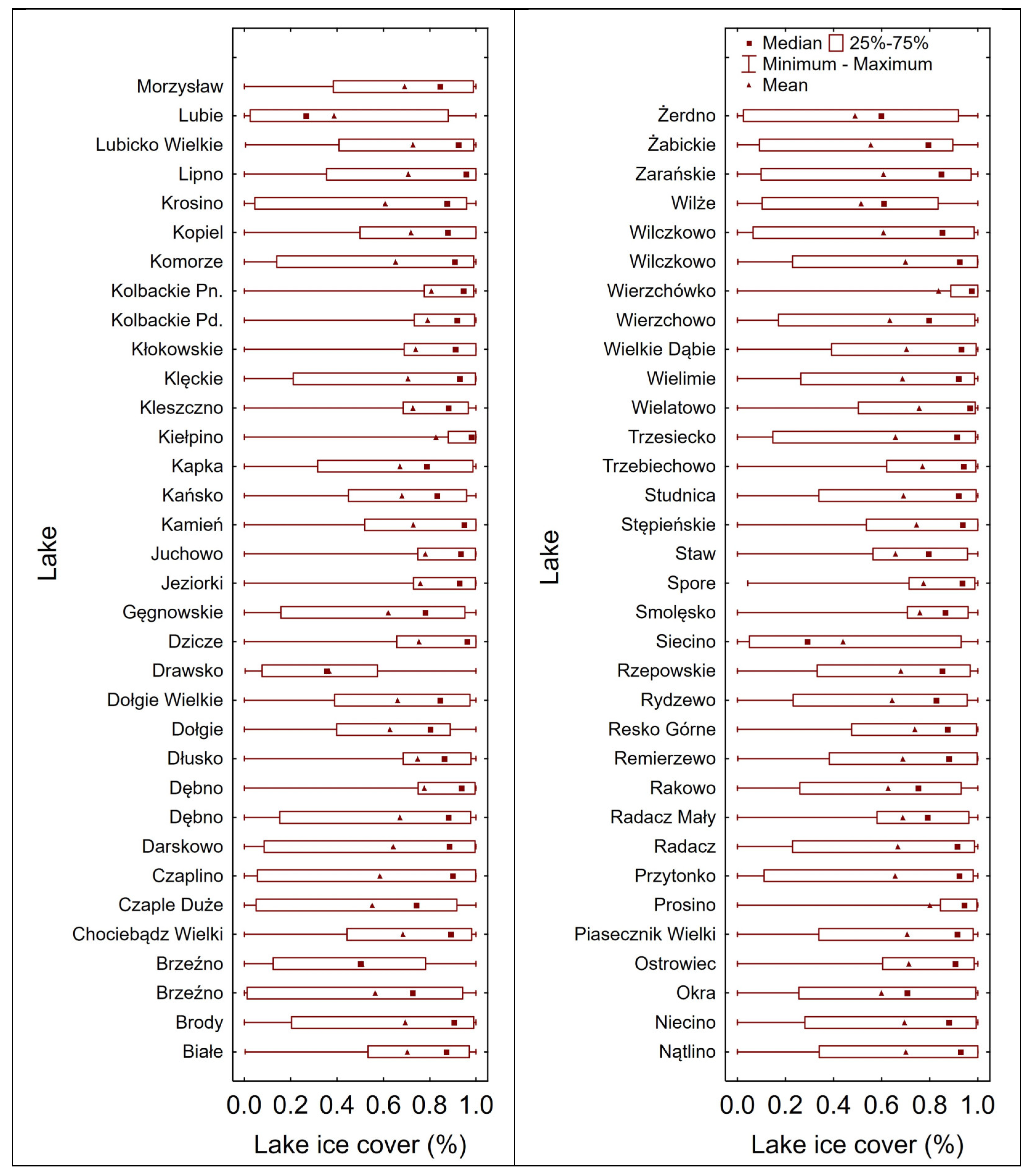
Considering the variability in ice cover on particular lakes, it was revealed that it changed in a range from 0 (no ice cover) to 1 (full ice cover). The mean value of ice cover on lakes was at a level from 0.37 (Lake Drawsko) to 0.84 (Lake Wierzchnówko), and the median value was from 0.27 (Lake Lubie) to 0.98 (Lake Kiełpino) (Figure 4).
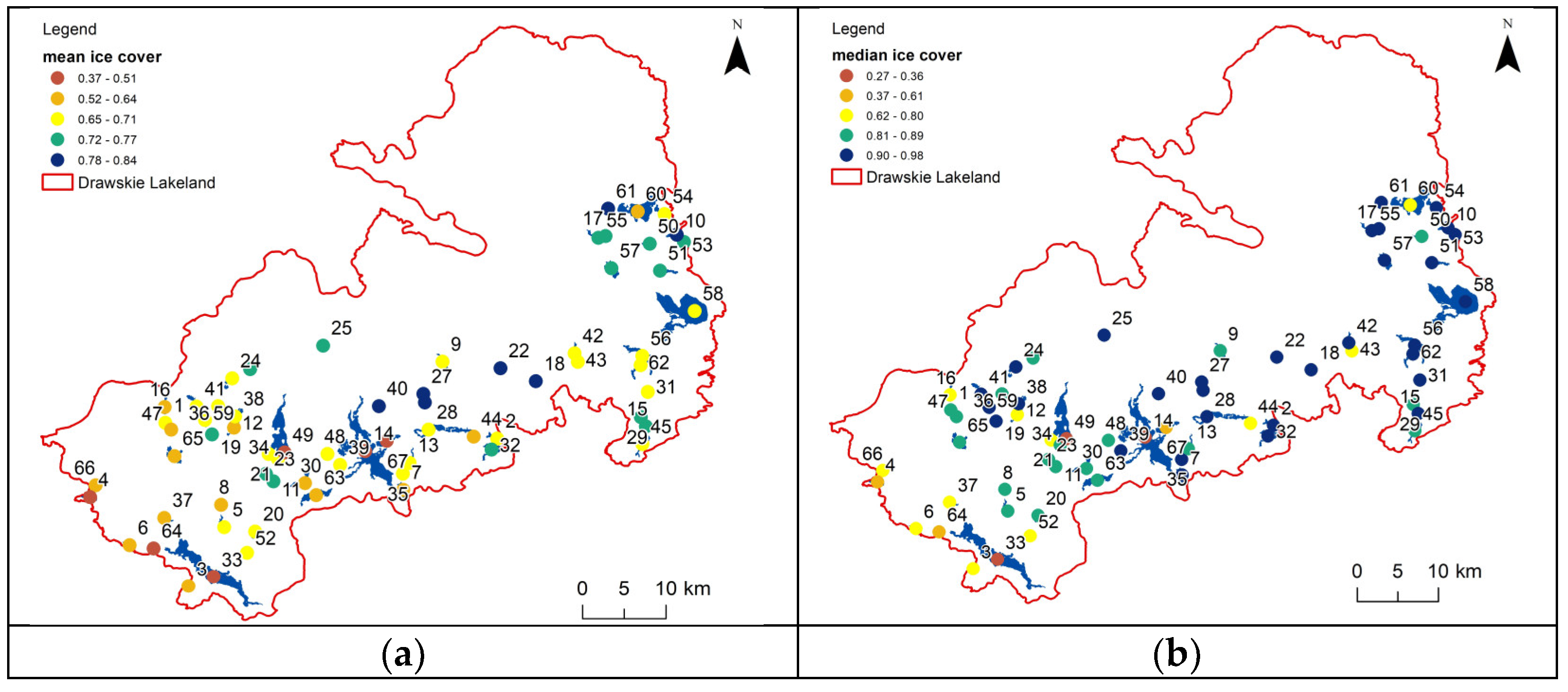
The spatial distribution of mean ice cover on lakes and the median values are presented in Figure 5. West of Lake Drawsko, there are generally lakes with mean ice values ranging from 0.37 to 0.64, while east of it, there are mostly lakes with mean ice values ranging from 0.72 to 0.84 (Figure 5a). A similar tendency occurs with respect to median values. West of Lake Drawsko, there are lakes with median values of ice cover from 0.90 to 0.98, and east of it, there are lakes with median values of ice cover from 0.27 to 0.80 (Figure 5b).
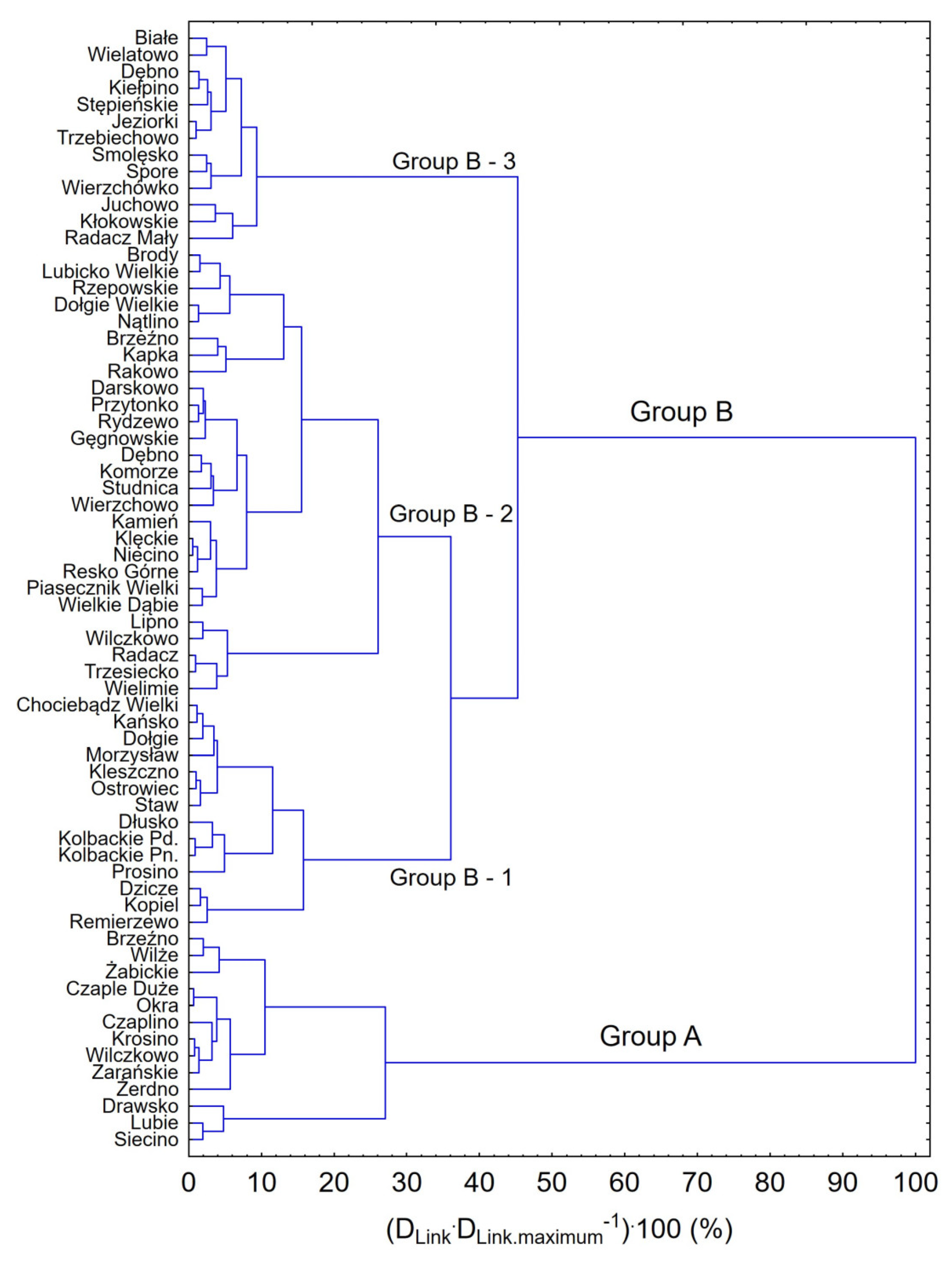
Data on the occurrence of ice cover for particular lakes were used in the cluster analysis, aiming to group lakes depending on the degree of ice cover observed in subsequent scenes from Landsat satellites. The obtained results showed that the analysed lakes could be divided into two groups, A and B. Group A included 13 lakes, and group B 54 lakes (Figure 6). In group B, three subgroups of lakes characterised by a different range of occurrence of ice cover were designated. Group B-1 included 14 lakes, group B-2—27 lakes, and group B-3—13 lakes.
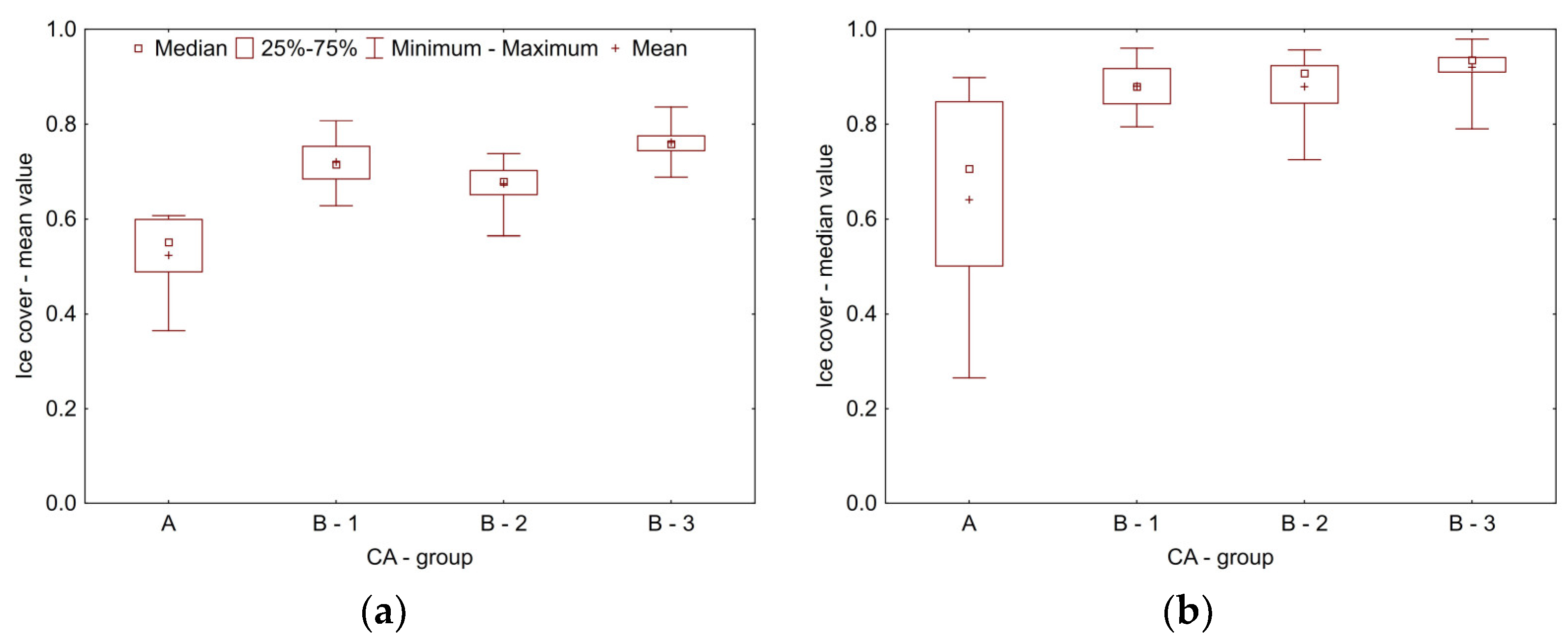
For lakes classified into group A, average ice cover varied from 0.37 to 0.61 (mean 0.52), and the median value was from 0.27 to 0.90 (mean 0.64). For lakes in group B, the ice cover values ranged from 0.56 to 0.84, and the median values from 0.73 to 0.98. Within particular subgroups, degrees of ice cover averaged from 0.63 to 0.81 for B-1, from 0.56 to 0.74 for B-2, and from 0.69 to 0.84 for B-3. The occurrence of ice cover within the designated groups and subgroups is presented in Figure 7. The statistical analysis of these results by means of a nonparametric Mann–Whitney U test showed that the average ice cover values in particular groups and subgroups differed at a significance level of 0.05. Considering the median values, no differences were found between groups B-1 and B-2, or between B-1 and B-3.
3.3. Factors Affecting the Lake Ice Cover Diversity
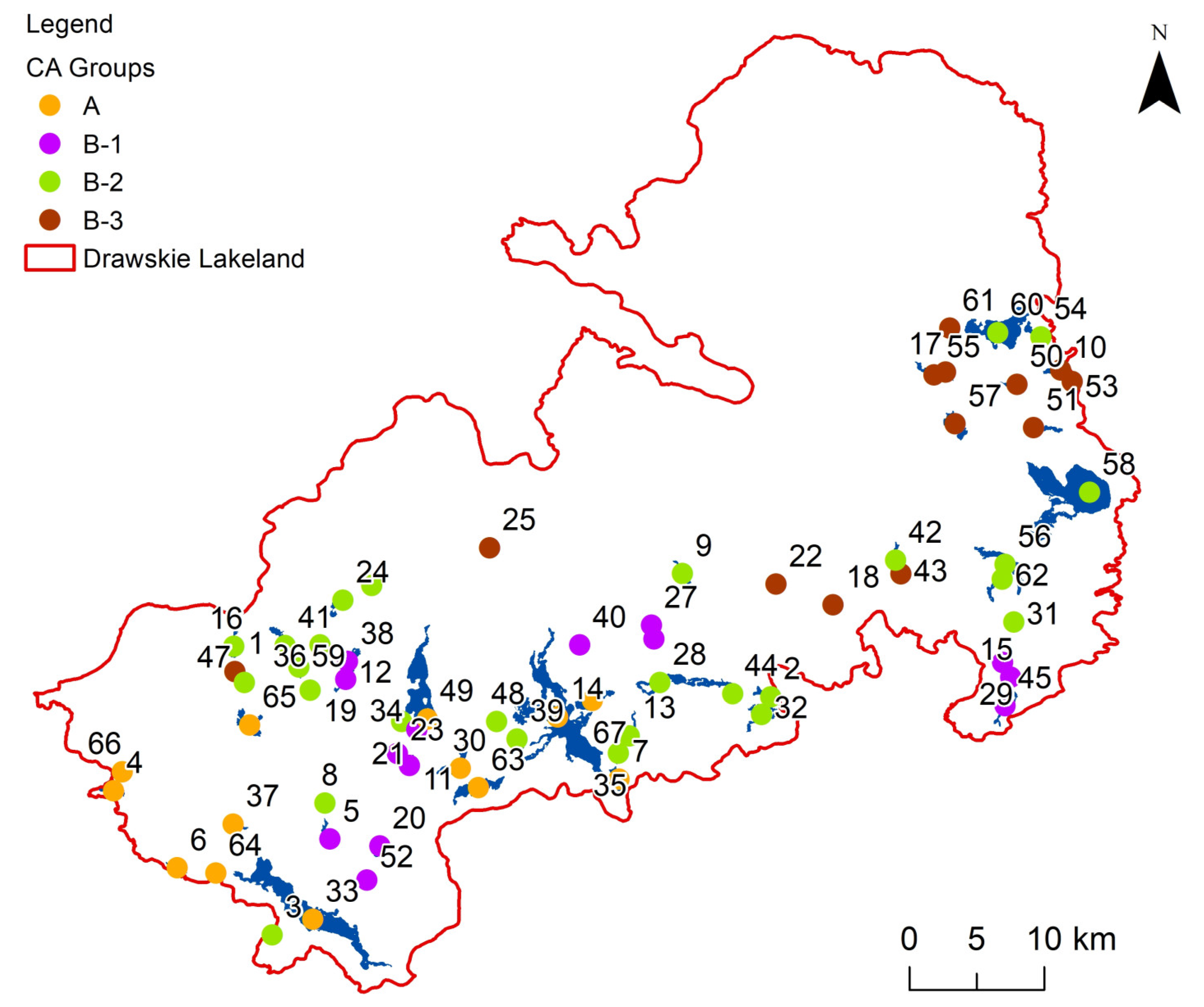
The analysis of lake morphometric parameters in particular groups designated by means of the CA method showed that group A includes lakes with the largest surface area, mean and maximum depth, volume, length, and width. The lakes also show the lowest altitude. The differences are statistically significant at the significance level of 0.05 (Table 1). Significant differences in morphometric parameters occur between subgroups B-1 and B-2. Subgroup B-2 includes lakes with almost all morphometric parameters showing values higher than those in lakes categorised to subgroup B-1, with the exception of altitude, maximum width, and exposure index. Lakes included in subgroups B-2 and B-3 differ only in terms of height of location, maximum and mean depth, and shoreline development index. No significant differences in morphometric parameters occur between lakes classified into subgroups B-1 and B-3. The spatial projection of results of the CA analysis revealed that lakes included in subgroups B-1 and B-3 are diverse in terms of location (Figure 8). Lakes included in subgroup B-1 are generally located in the west of the Drawskie Lakeland, and those in subgroup B-3 in the east.
The principal component analysis showed that parameters that differentiate the degree of ice cover between the analysed lakes included surface area, lake volume, maximum and mean depth, shoreline length, and height of the lake’s location above sea level (Figure 9). For lakes located at the lowest height, less ice cover was recorded, and lakes with high values of surface area, volume, maximum and mean depth, and shoreline length showed less ice cover.
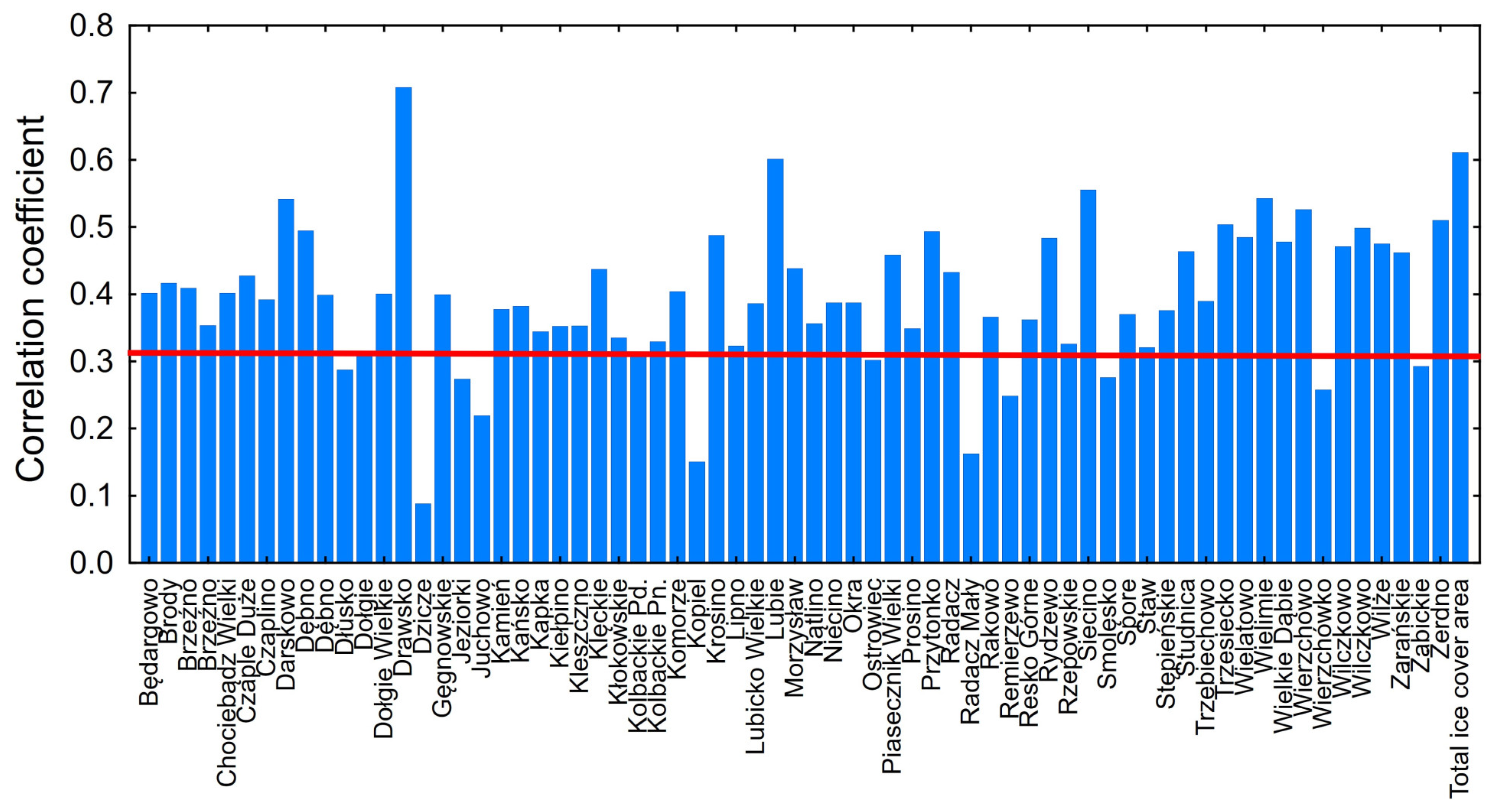
The determination of the correlation between ice cover and climate conditions involved the analysis of the dependency of its surface area on accumulated freezing degree days (AFDD). AFDD constitutes the result of the accumulation of freezing temperatures for a given season (with consideration of snowmelt), and is a parameter commonly used in research on ice cover on lakes [34,35,36]. The obtained results show a significant correlation between ice cover surface area and AFDD for 54 lakes (Figure 10). The highest value was obtained for the largest lakes, namely, Drawsko, Lubie, Siecino, and Wielimie, where the correlation coefficient values were 0.71, 0.60, 0.56, and 0.54, respectively. The total surface area of ice on all the analysed lakes also correlated with AFDD at a level of 0.61. Some limitations of the obtained results may be due to the distance of the Piła station outside of the Drawsko Lakeland area and the fact, that during the calculations, no lapse rate adjustment was used to adjust the temperature from the Piła station elevation to the lakes’ elevations. On the other hand, air temperature showed high correlations with the temperature of the surface water layer (for monitored lakes: Drawsko, Lubie, Komorze), i.e., in the zone where ice cover develops.
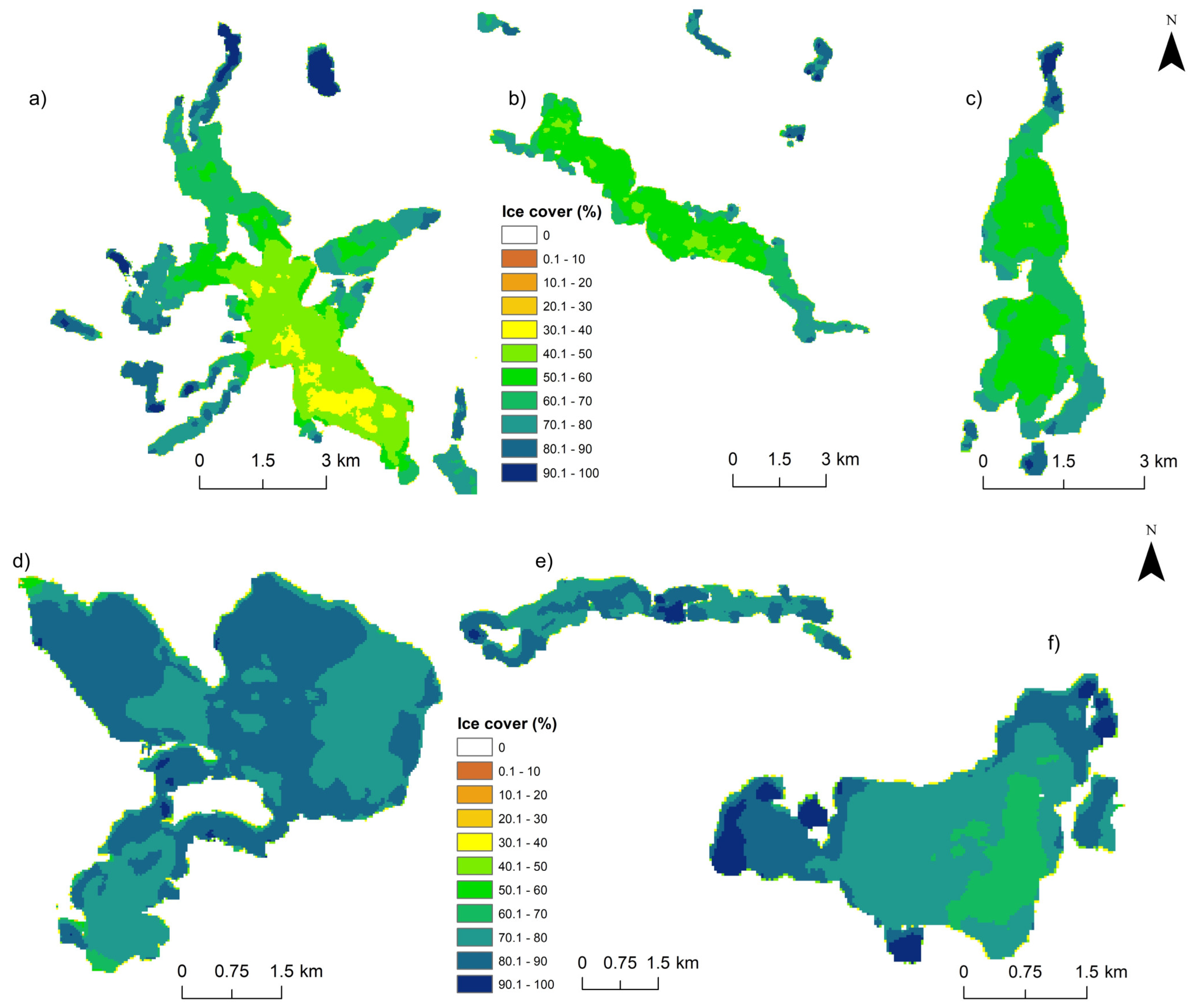
The analysis of the spatial range of ice occurrence on particular lakes from subsequent terms permitted the preparation of maps presenting the probability of occurrence of ice cover in reference to the largest lakes in the study area (Figure 11).
The results show a higher probability of occurrence of ice cover for lakes Komorze, Wielimie, and Wierzchowo than for lakes Drawsko, Lubie, and Siecino. Such a situation largely depends on the surface area and depth of individual lakes. In Lake Drawsko, in some areas of its central part, ice cover occurred only in 30–40% of the analysed Landsat satellite images. Ice cover was most frequently encountered in the narrowest northern and northwestern bays. On the other hand, Lake Wielimie, with a surface area approximate to that of Lake Drawsko, but with a smaller depth (mean depth = 2.2 m), showed a high probability of occurrence of ice cover.
Observations of ice cover in Polish lakes conducted to date have been based on in situ measurements, and cover a group of only several tens of lakes, narrowed down to objects with large surface areas. This context reveals a gap in reference to smaller lakes (the most abundant), important from the point of view of the functioning of the catchments in which they occur. So far, in the times of dynamic, or even explosive, development of teledetection, the tools have not been so far applied for the assessment of ice conditions in Polish lakes. It should also be emphasised that research on ice cover on lakes in many regions around the globe currently uses increasingly advanced remote sensing techniques [37] providing accurate and detailed information on the subject. The remote sensing of frozen rivers and lakes can, to a greater degree, contribute to the investigation of the role of water bodies in hydrology and effects of environmental variability and change in the ice and hydrological system [38].
In this context, research was undertaken aiming to determine the usefulness of publicly available Landsat images for the analysis of ice cover on Polish lakes. This research subject corresponds with earlier studies employing such images [39,40,41]. Landsat images permit the analysis of ice cover on small lakes, although according to Zhang and Pavelsky [42], certain limitations also exist resulting from the revisit time (16 days for Landsat 4 onwards), as well as the occurrence of cloudiness, additionally limiting the availability of data from the images. On the other hand, there is a simple possibility of ice detection based on Landsat satellites with simultaneous application of the rich archive of the images [43]. This is particularly important for areas such as Poland, where this type of analysis has never been conducted before. The results showed that the designated study area is characterised by high variability in ice cover on its lakes. Therefore, the relatively small surface area of the Drawskie Lakeland (with generally uniform climate conditions) clearly points to the individual parameters of lakes as key for the occurrence of ice cover. This statement is reflected in the statistical analyses and significance of particular morphometric parameters. Lakes with the largest surface area, the middle parts of which were covered with ice the most, seldom are the most prone to wind action. According to Ke et al. [44] the delay in terms of the freezing of Lake Khanka is strongly correlated with an increase in wind speed. In the case of Lake Ulansuhai (China), wind was the main driver of development of ice cover [45]. The role of wind for the course of ice cover in five lakes in Poland was assessed by Bartosiewicz et al. [46]. According to the authors, the effect of wind delays ice development in autumn. It should be emphasised that particular parameters combined provide conditions less or more favourable for the occurrence of ice cover in lakes. Research by Williams et al. [47] evidenced that surface area and mean depth are positively correlated with the appearance of ice cover. The spatial pattern of freezing and defrosting of Lake Qinghai may, to a certain degree, reflect the difference in water depth in the lake within the designated areas; in the west, similar spatial patterns of freezing and ablation occurred, whereas in the eastern part, they were reversed [36]. The analysis of more than a hundred lakes in Norway showed a considerable effect of lake surface area because small lakes froze earlier due to their smaller volume [48]. The analysis of the frequency and range of ice cover in Lower Lake Constance with three basins with variable morphology revealed that full ice cover occurs almost each winter in the shallowest part, most isolated, with no substantial inflows [49]. Situations described in the said study, pointing to the variability in ice cover within particular lakes, owing to remote sensing techniques, were, for the first time, conclusively confirmed for the selected Polish lakes. In bays, the shallowest zones of the lakes protected from wind, ice cover was recorded the most frequently, as evident in the case of lakes Drawsko, Lubie, Wierzchowo, and Siecino. In the case of the latter, Ostrów Island plays a considerable role (in the southeastern part). It isolates the part of the lake with recorded high frequency of occurrence of ice cover. The image of spatial occurrence of ice cover in Lake Wielimie is interesting. Despite its large surface area, but simultaneously low mean depth, it maintains a relatively uniform distribution in terms of this characteristic. Two zones deserve particular attention. The first one is the northwestern part of the lake—the mouth zone of the Gwda River—where the probability of occurrence of ice cover is at a level of 50–60% (Figure 11c). The determination of the interaction between river flow and ice cover corresponds with earlier studies of the type, where, among others in the case of the Great Slave Lake, the inflow of the Slave River plays a substantial role in the occurrence of ice cover [50]. The second characteristic zone in Lake Wielimie is its southwestern part with the inflow of the urban Nizica River. Flowing through an urbanised area (Szczecinek), the river supplies waters with different physicochemical properties than those in the lake. In the winter period, the supply of salt used for snowploughing roads and pavements is important. With surface flow, it is supplied to the urban river and then reaches Lake Wielimie. The role of anthropogenic pollutants for the development of ice cover in water bodies was emphasised by Stolarski and Rzetała [51]. According to the authors, in such conditions, the ice layer does not form at all (even in the conditions of a substantial decrease in air temperature), or it is very thin.
The importance of ice cover on lakes is particularly great in the context of global warming, where numerous studies point to changes in the ice regime [52,53,54], and the situation is considered an evident indicator of climate change [55,56]. The changes will progress over the next several decades [46,57], considerably changing the current lake parameters shaped by the presence of ice cover. It is therefore important to use all the available techniques and possibilities of monitoring the distribution and course of ice cover on lakes. The issue is of importance not only in reference to cases subject to continuous observations, but also for ones to which such an approach is not applied. Appropriate decision making in the scope of water management and activities aiming to optimise of the functioning of lake ecosystems in the scope of both biotic and abiotic conditions requires detailed knowledge, and, as evidenced by the obtained results, remote sensing techniques can constitute an important source of information for Polish lakes.
4. Conclusions
Observations of ice cover in Polish lakes conducted to date provide several-decades-long datasets, and are based on field measurements. They generally refer to lakes with relatively large surface areas covering a total of several tens of lakes, which is a small group in the context of the entire population. Remote sensing techniques have not been applied so far, whereas their importance and accuracy in data collection is dynamically increasing on a year-to-year basis in different regions of the globe. Satellite images from the Landsat mission permitted the description of ice cover in lakes never monitored before in those terms (mainly small ones), and the assessment of the spatial variability in the occurrence of ice cover within individual lakes. Despite the relatively small study area, considerable variability in the occurrence of ice cover was found, and the morphometric parameters of lakes proved key in this aspect. The implementation of the methodical assumptions referring to satellite images and the obtained results offers new possibilities in the context of expanding knowledge on the occurrence of ice in Polish lakes. In the times of climate change and the progressing transformation of the natural environment, this approach is complementary for activities in the scope of the management of lake ecosystems, in reference to both biotic and abiotic aspects. In the case of multitemporal analyses, attention should be paid to changes in water surface area caused by changes in water levels and overgrowth. Changes in water level in moraine lakes and coastal lakes with smooth shores can significantly affect the surface of the water table and the results of ice cover analysis based on satellite data. In tunnel lakes with steep shores, changes in water level affect the surface of the water table and, therefore, the analysis results, to a lower extent.
Supplementary Materials
The following supporting information can be downloaded at: https://www.mdpi.com/article/10.3390/rs15123030/s1, Table S1: Morphometric parameters of the studied lakes.
Author Contributions
Conceptualisation, M.S. and M.P.; methodology, M.S.; software, M.S.; validation, M.S.; formal analysis, M.S.; investigation, M.S.; resources, M.S.; data curation, M.S.; writing—original draft preparation, M.S. and M.P. writing—review and editing, M.S., M.P. and S.Z. visualization, M.S.; supervision, M.S., M.P. and S.Z.; project administration, M.P.; funding acquisition, M.P., M.S. and S.Z. All authors have read and agreed to the published version of the manuscript.
Funding
This research received no external funding.
Data Availability Statement
Data used in this study are available upon reasonable request from the corresponding author.
Conflicts of Interest
The authors declare no conflict of interest.
References
- Bai, Q.; Li, R.; Li, Z.; Leppäranta, M.; Arvola, L.; Li, M. Time-series analyses of water temperature and dissolved oxygen concentration in Lake Valkea-Kotinen (Finland) during ice season. Ecol. Inform. 2016, 36, 181–189. [Google Scholar] [CrossRef]
- Bengtsson, L.; Ali-Maher, O. The dependence of the consumption of dissolved oxygen on lake morphology in ice covered lakes. Hydrol. Res. 2020, 51, 381–391. [Google Scholar] [CrossRef]
- Roulet, N.T.; Adams, W.P. Spectral distribution of light under a subarctic winter lake cover. Hydrobiologia 1986, 134, 89–95. [Google Scholar] [CrossRef]
- Bramburger, A.J.; Ozersky, T.; Silsbe, G.M.; Crawford, C.; Olmanson, L.G.; Shchapov, K. The not-so-dead of winter: Underwater light climate and primary productivity under snow and ice cover in inland lakes. Inland Waters 2022, 13, 1–12. [Google Scholar] [CrossRef]
- Huang, W.; Zhang, Z.; Li, Z.; Leppäranta, M.; Arvola, L.; Song, S.; Huotari, J.; Lin, Z. Under-ice dissolved oxygen and metabolism dynamics in a shallow lake: The critical role of ice and snow. Water Resour. Res. 2021, 57, e2020WR027990. [Google Scholar] [CrossRef]
- Choiński, A.; Ptak, M.; Strzelczak, A. Changeability of accumulated heat content in alpine-type lakes. Pol. J. Environ. Stud. 2015, 24, 2363–2369. [Google Scholar] [CrossRef]
- Yang, F.; Li, C.; Leppäranta, M.; Shi, X.; Zhao, S.; Zhang, C. Notable increases in nutrient concentrations in a shallow lake during seasonal ice growth. Water Sci. Technol. 2016, 74, 2773–2783. [Google Scholar] [CrossRef] [Green Version]
- Huang, C.; Zhu, L.; Ma, G.; Meadows, G.A.; Xue, P. Wave Climate Associated with Changing Water Level and Ice Cover in Lake Michigan. Front. Mar. Sci. 2021, 8, 746916. [Google Scholar] [CrossRef]
- Chiapella, A.M.; Grigel, H.; Lister, H.; Hrycik, A.; O’Malley, B.P.; Stockwell, J.D. A day in the life of winter plankton: Under-ice community dynamics during 24 h in a eutrophic lake. J. Plankton Res. 2021, 43, 865–883. [Google Scholar] [CrossRef]
- Hrycik, A.R.; McFarland, S.; Morales-Williams, A.; Stockwell, J.D. Winter severity shapes spring plankton succession in a small, eutrophic lake. Hydrobiologia 2022, 849, 2127–2144. [Google Scholar] [CrossRef]
- Pöysä, H. Local variation in the timing and advancement of lake ice breakup and impacts on settling dynamics in a migratory waterbird. Sci. Total Environ. 2022, 811, 151397. [Google Scholar] [CrossRef] [PubMed]
- Choiński, A. Katalog Jezior Polski; Wydawnictwo Naukowe UAM: Poznań, Poland, 2006. [Google Scholar]
- Ptak, M.; Choiński, A.; Strzelczak, A.; Targosz, A. Disappearance of Lake Jelenino since the end of the XVIII century as an effect of anthropogenic transformations of the natural environment. Pol. J. Environ. Stud. 2013, 22, 191–196. [Google Scholar]
- Barańczuk, K.; Barańczuk, J. Formulas for calculating ice cover thickness on selected spring lakes on the upper Radunia (Kashubian Lakeland, northern Poland). Limnol. Rev. 2020, 20, 199–205. [Google Scholar] [CrossRef]
- Machowski, R. Course of ice phenomena in small water reservoir in Katowice (Poland) in the winter season 2011/2012. Environ. Socio-Econ. Stud. 2013, 1, 7–13. [Google Scholar] [CrossRef] [Green Version]
- Nowak, B.; Nowak, D.; Ptak, M. Variability and course of occurrence of ice cover on selected lakes of the Gnieźnieńskie Lakeland (Central Poland) in the period 1976–2015. E3S Web Conf. 2018, 44, 00126. [Google Scholar] [CrossRef]
- Ptak, M.; Sojka, M.; Nowak, B. Changes in ice regime of Jagodne Lake (North-Eastern Poland). Acta Sci. Pol. Form. Circumiectus 2019, 18, 89–100. [Google Scholar] [CrossRef]
- Solarski, M.; Rzetala, M. Ice Regime of the Kozłowa Góra Reservoir (Southern Poland) as an Indicator of Changes of the Thermal Conditions of Ambient Air. Water 2020, 12, 2435. [Google Scholar] [CrossRef]
- Wrzesiński, D.; Choiński, A.; Ptak, M.; Skowron, R. Effect of the North Atlantic Oscillation on the Pattern of Lake Ice Phenology in Poland. Acta Geophys. 2015, 63, 1664–1684. [Google Scholar] [CrossRef] [Green Version]
- Warne, C.P.K.; McCann, K.S.; Rooney, N.; Cazelles, K.; Guzzo, M.M. Geography and Morphology Affect the Ice Duration Dynamics of Northern Hemisphere Lakes Worldwide. Geophys. Res. Lett. 2020, 47, e2020GL087953. [Google Scholar] [CrossRef]
- Heinilä, K.; Mattila, O.-P.; Metsämäki, S.; Väkevä, S.; Luojus, K.; Schwaizer, G.; Koponen, S. A novel method for detecting lake ice cover using optical satellite data. Int. J. Appl. Earth Obs. Geoinf. 2021, 104, 102566. [Google Scholar] [CrossRef]
- Wu, Y.; Duguay, C.R.; Xu, L. Assessment of machine learning classifiers for global lake ice cover mapping from MODIS TOA reflectance data. Remote Sens. Environ. 2021, 253, 112206. [Google Scholar] [CrossRef]
- Wang, J.; Duguay, C.R.; Clausi, D.A.; Pinard, V.; Howell, S.E.L. Semi-automated classification of Lake Ice Cover using dual polarization RADARSAT-2 imagery. Remote Sens. 2018, 10, 1727. [Google Scholar] [CrossRef] [Green Version]
- Dastour, H.; Ghaderpour, E.; Hassan, Q.K. A Combined Approach for Monitoring Monthly Surface Water/Ice Dynamics of Lesser Slave Lake via Earth Observation Data. IEEE J. Sel. Top. Appl. Earth Obs. Remote Sens. 2022, 15, 6402–6417. [Google Scholar] [CrossRef]
- Herrick, C.; Steele, B.G.; Brentrup, J.A.; Cottingham, K.L.; Ducey, M.J.; Lutz, D.A.; Palace, M.W.; Thompson, M.C.; Trout-Haney, J.V.; Weathers, K.C. lakeCoSTR: A tool to facilitate use of Landsat Collection 2 to estimate lake surface water temperatures. Ecosphere 2023, 14, e4357. [Google Scholar] [CrossRef]
- Jańczak, J. (Ed.) Atlas Jezior Polski. Jeziora Pojezierza Wielkopolskiego i Pomorskiego w Granicach Dorzecza Odry; Bogucki Wydawnictwo Naukowe: Poznań, Poland, 1996. [Google Scholar]
- Foga, S.; Scaramuzza, P.L.; Guo, S.; Zhu, Z.; Dilley, R.D.; Beckmann, T.; Schmidt, G.L.; Dwyer, J.L.; Hughes, M.J.; Laue, B. Cloud detection algorithm comparison and validation for operational Landsat data products. Remote Sens. Environ. 2017, 194, 379–390. [Google Scholar] [CrossRef] [Green Version]
- Daniels, R.C. Using ArcMap to extract shorelines from Landsat TM & ETM+ data. In Proceedings of the 32nd ESRI International Users Conference, San Diego, CA, USA, 23–27 July 2012; pp. 23–27. [Google Scholar]
- Ihlen, V. Landsat 8 Data Users Handbook; U.S. Geological Survey: Sioux Falls, SD, USA, 2019. [Google Scholar]
- Cáceres, A.; Schwarz, E.; Aldenhoff, W. Landsat-8 Sea Ice Classification Using Deep Neural Networks. Remote Sens. 2022, 14, 1975. [Google Scholar] [CrossRef]
- McFeeters, S.K. The use of the Normalized Difference Water Index (NDWI) in the delineation of open water features. Int. J. Remote Sens. 1996, 17, 1425–1432. [Google Scholar] [CrossRef]
- Richter, R.; Schläpfer, D. Atmospheric and Topographic Correction (ATCOR Theoretical Background Document); DLR—German Aerospace Center: Wessling, Germany, 2021. [Google Scholar]
- Liu, C.W.; Lin, K.H.; Kuo, Y.M. Application of factor analysis in the assessment of groundwater quality in blackfoot disease in Taiwan. Sci. Total Environ. 2003, 313, 77–89. [Google Scholar] [CrossRef]
- Beyene, M.T.; Jain, S. Wintertime weather-climate variability and its links to early spring ice-out in Maine Lakes. Limnol. Oceanogr. 2015, 60, 1890–1905. [Google Scholar] [CrossRef] [Green Version]
- Karetnikov, S.; Leppäranta, M.; Montonen, A. A time series of over 100 years of ice seasons on Lake Ladoga. J. Great Lakes Res. 2017, 43, 979–988. [Google Scholar] [CrossRef]
- Qi, M.; Liu, S.; Yao, X.; Xie, F.; Gao, Y. Monitoring the Ice Phenology of Qinghai Lake from 1980 to 2018 Using Multisource Remote Sensing Data and Google Earth Engine. Remote Sens. 2020, 12, 2217. [Google Scholar] [CrossRef]
- Cai, Y.; Ke, C.-Q.; Duan, Z. Monitoring ice variations in Qinghai Lake from 1979 to 2016 using passive microwave remote sensing data. Sci. Total Environ. 2017, 607–608, 120–131. [Google Scholar] [CrossRef] [PubMed]
- Jeffries, M.O.; Morris, K.; Kozlenko, N. Ice characteristics and processes, and remote sensing of frozen rivers and lakes. Geophys. Monogr. Ser. 2005, 163, 63–90. [Google Scholar] [CrossRef]
- Leshkevich, G.A. Machine classification of freshwater ice types from Landsat-I digital data using ice albedos as training sets. Remote Sens. Environ. 1985, 17, 251–263. [Google Scholar] [CrossRef]
- Jin, H.; Gan, T.; Zeng, B.; Song, X.; Chen, J. Namco Lake Ice Detection from Landsat-8 Imagery with Improved Deeplab v3+. In Proceedings of the CTISC 2022—2022 4th International Conference on Advances in Computer Technology, Information Science and Communications, Suzhou, China, 22–24 April 2022. [Google Scholar] [CrossRef]
- Cook, T.L.; Bradley, R.S. An analysis of past and future changes in the ice cover of two high-arctic lakes based on synthetic aperture radar (SAR) and Landsat imagery. Arct. Antarct. Alp. Res. 2010, 42, 9–18. [Google Scholar] [CrossRef]
- Zhang, S.; Pavelsky, T.M. Remote Sensing of Lake Ice Phenology across a Range of Lakes Sizes, ME, USA. Remote Sens. 2019, 11, 1718. [Google Scholar] [CrossRef] [Green Version]
- Yang, X.; Pavelsky, T.M.; Bendezu, L.P.; Zhang, S. Simple Method to Extract Lake Ice Condition from Landsat Images. IEEE Trans. Geosci. Remote Sens. 2022, 60, 1–10. [Google Scholar] [CrossRef]
- Ke, C.; Cai, Y.; Xiao, Y. Monitoring ice phenology variations in Khanka Lake based on passive remote sensing data from 1979 to 2019. Natl. Remote Sens. Bull. 2022, 26, 201–210. [Google Scholar]
- Yang, F.; Feng, W.; Leppäranta, M.; Yang, Y.; Merkouriadi, I.; Cen, R.; Bai, Y.; Li, C.; Liao, H. Simulation and seasonal characteristics of the intra-annual heat exchange process in a shallow ice-covered lake. Sustainability 2020, 12, 7832. [Google Scholar] [CrossRef]
- Bartosiewicz, M.; Ptak, M.; Woolwey, I.; Sojka, M. On thinning ice: Effects of atmospheric warming, stilling and rainfall intensity on ice conditions in differently shaped lakes. J. Hydrol. 2021, 597, 125724. [Google Scholar] [CrossRef]
- Williams, G.; Layman, K.L.; Stefan, H.G. Dependence of lake ice covers on climatic, geographic and bathymetric variables. Cold Reg. Sci. Technol. 2004, 40, 145–164. [Google Scholar] [CrossRef]
- L’Abée-Lund, J.H.; Vøllestad, L.A.; Brittain, J.E.; Kvambekk, A.S.; Solvang, T. Geographic variation and temporal trends in ice phenology in Norwegian lakes during the period 1890–2020. Cryosphere 2021, 15, 2333–2356. [Google Scholar] [CrossRef]
- Caramatti, I.; Peeters, F.; Hamilton, D.; Hofmann, H. Modelling inter-annual and spatial variability of ice cover in a temperate lake with complex morphology. Hydrol. Process. 2020, 34, 691–704. [Google Scholar] [CrossRef] [Green Version]
- Howell, S.E.L.; Brown, L.C.; Kang, K.-K.; Duguay, C.R. Variability in ice phenology on Great Bear Lake and Great Slave Lake, Northwest Territories, Canada, from SeaWinds/QuikSCAT: 2000–2006. Remote Sens. Environ. 2009, 113, 816–834. [Google Scholar] [CrossRef]
- Solarski, M.; Rzetala, M. Changes in the Thickness of Ice Cover on Water Bodies Subject to Human Pressure (Silesian Upland, Southern Poland). Front. Earth Sci. 2021, 920, 675216. [Google Scholar] [CrossRef]
- Kainz, M.J.; Ptacnik, R.; Rasconi, S.; Hager, H.H. Irregular changes in lake surface water temperature and ice cover in subalpine Lake Lunz, Austria. Inland Waters 2017, 7, 27–33. [Google Scholar] [CrossRef]
- Christianson, K.R.; Loria, K.A.; Blanken, P.D.; Caine, N.; Johnson, P.T.J. On thin ice: Linking elevation and long-term losses of lake ice cover. Limnol. Oceanogr. Lett. 2021, 6, 77–84. [Google Scholar] [CrossRef]
- Newton, A.M.W.; Mullan, D.J. Climate change and Northern Hemisphere lake and river ice phenology from 1931–2005. Cryosphere 2021, 15, 2211–2234. [Google Scholar] [CrossRef]
- Ptak, M.; Sojka, M.; Nowak, B. Effect of climate warming on a change in thermal and ice conditions in the largest lake in Poland—Lake Śniardwy. J. Hydrol. Hydrodyn. 2020, 68, 260–270. [Google Scholar] [CrossRef]
- Ptak, M.; Sojka, M. The disappearance of ice cover on temperate lakes (Central Europe) as a result of global warming. Geogr. J. 2021, 187, 200–213. [Google Scholar] [CrossRef]
- Huang, L.; Timmermann, A.; Lee, S.-S.; Rodgers, K.B.; Yamaguchi, R.; Chung, E.-S. Emerging unprecedented lake ice loss in climate change projections. Nat. Commun. 2022, 13, 5798. [Google Scholar] [CrossRef] [PubMed]
Figure 1.
Study site location.

Figure 2.
Number of available satellite scenes used in the paper for the analysis of ice cover on lakes in reference to particular hydrological years (a) in reference to satellites (b) and months (c).
Figure 2.
Number of available satellite scenes used in the paper for the analysis of ice cover on lakes in reference to particular hydrological years (a) in reference to satellites (b) and months (c).

Figure 3.
Variability in ice cover on lakes in the analysed scenes (scenes with partial ice cover).

Figure 4.
Variability in ice cover on lakes of the Drawskie Lakeland in scenes from Landsat satellites from the period 1986–2022.
Figure 4.
Variability in ice cover on lakes of the Drawskie Lakeland in scenes from Landsat satellites from the period 1986–2022.

Figure 5.
Mean values (a) and medians (b) of ice cover calculated based on Landsat data from the period 1986–2022.
Figure 5.
Mean values (a) and medians (b) of ice cover calculated based on Landsat data from the period 1986–2022.

Figure 6.
Division of lakes into groups by ice cover range.

Figure 7.
Average (a) and median values (b) of ice cover in groups of lakes designated by means of the CA method.
Figure 7.
Average (a) and median values (b) of ice cover in groups of lakes designated by means of the CA method.

Figure 8.
Spatial distribution of lakes classified to groups A, B-1, B-2, and B-3 within the Drawskie Lakeland.
Figure 8.
Spatial distribution of lakes classified to groups A, B-1, B-2, and B-3 within the Drawskie Lakeland.

Figure 9.
Effect of morphometric factors on the occurrence of ice cover on the analysed lakes.

Figure 10.
Correlation coefficient between ice cover surface area on lakes and accumulated freezing degree days (AFDD) (The red line represents the correlation significance threshold at the significance level of 0.05).
Figure 10.
Correlation coefficient between ice cover surface area on lakes and accumulated freezing degree days (AFDD) (The red line represents the correlation significance threshold at the significance level of 0.05).

Figure 11.
Probability of occurrence of ice cover on lakes: Drawsko (a), Lubie (b), Siecino (c), Wielimie (d), Komorze (e), and Wierzchowo (f).
Figure 11.
Probability of occurrence of ice cover on lakes: Drawsko (a), Lubie (b), Siecino (c), Wielimie (d), Komorze (e), and Wierzchowo (f).


Table 1.
Differences between morphometric parameters of lakes within groups designated by means of the CA method.
Table 1.
Differences between morphometric parameters of lakes within groups designated by means of the CA method.
| Parameters | A vs. B-1 | A vs. B-2 | A vs. B-3 | B-1 vs. B-2 | B-1 vs. B-3 | B-2 vs. B-3 |
|---|---|---|---|---|---|---|
| Area (ha) | 1 | 1 | 1 | −1 | 0 | 0 |
| Altitude (m asl) | −1 | −1 | −1 | 0 | 0 | −1 |
| Volume (106 m3) | 1 | 1 | 1 | −1 | 0 | 0 |
| Mean depth (m) | 1 | 1 | 1 | −1 | 0 | 1 |
| Maximum depth (m) | 1 | 1 | 1 | −1 | 0 | 1 |
| Maximum length (m) | 1 | 1 | 1 | −1 | 0 | 0 |
| Maximum width (m) | 1 | 1 | 1 | 0 | 0 | 0 |
| Effective length (m) | 1 | 1 | 1 | −1 | 0 | 0 |
| Shoreline length (m) | 1 | 0 | 1 | −1 | 0 | 0 |
| Shoreline development index (-) | 0 | 0 | 0 | −1 | 0 | 1 |
| Exposure index (-) | 0 | 0 | 0 | 0 | 0 | 0 |
1—significantly higher A value than B at level 0.05, 0—no differences, −1—significantly lower A value than B at level 0.05.
Disclaimer/Publisher’s Note: The statements, opinions and data contained in all publications are solely those of the individual author(s) and contributor(s) and not of MDPI and/or the editor(s). MDPI and/or the editor(s) disclaim responsibility for any injury to people or property resulting from any ideas, methods, instructions or products referred to in the content. |
© 2023 by the authors. Licensee MDPI, Basel, Switzerland. This article is an open access article distributed under the terms and conditions of the Creative Commons Attribution (CC BY) license (https://creativecommons.org/licenses/by/4.0/).
Share and Cite
MDPI and ACS Style
Sojka, M.; Ptak, M.; Zhu, S. Use of Landsat Satellite Images in the Assessment of the Variability in Ice Cover on Polish Lakes. Remote Sens. 2023, 15, 3030. https://doi.org/10.3390/rs15123030
AMA Style
Sojka M, Ptak M, Zhu S. Use of Landsat Satellite Images in the Assessment of the Variability in Ice Cover on Polish Lakes. Remote Sensing. 2023; 15(12):3030. https://doi.org/10.3390/rs15123030
Chicago/Turabian StyleSojka, Mariusz, Mariusz Ptak, and Senlin Zhu. 2023. "Use of Landsat Satellite Images in the Assessment of the Variability in Ice Cover on Polish Lakes" Remote Sensing 15, no. 12: 3030. https://doi.org/10.3390/rs15123030
Note that from the first issue of 2016, this journal uses article numbers instead of page numbers. See further details here.