
Unambiguous Wind Direction Estimation Method for Shipborne HFSWR Based on Wind Direction Interval Limitation


1
First Institute of Oceanography, Ministry of Natural Resources, Qingdao 266001, China
2
College of Engineering, Ocean University of China, Qingdao 266100, China
3
College of Oceanography and Space Informatics, China University of Petroleum (East China), Qingdao 266580, China
*
Author to whom correspondence should be addressed.
Remote Sens. 2023, 15(11), 2952; https://doi.org/10.3390/rs15112952
Submission received: 17 March 2023
/
Revised: 19 May 2023
/
Accepted: 22 May 2023
/
Published: 5 June 2023
(This article belongs to the Special Issue Feature Paper Special Issue on Ocean Remote Sensing - Part 2)
Abstract
:Due to its maneuverability and agility, the shipborne high-frequency surface wave radar (HFSWR) provides a new way of monitoring large-area marine dynamics and environment information. However, wind direction ambiguity is problematic when using monostatic shipborne HFSWR for wind direction inversion. In this article, an unambiguous wind direction measurement method based on wind direction interval limitation is proposed. The two first-order spectral wind direction estimation methods are first presented using the relationship between the normalized amplitude differences or ratios of the broadened Doppler spectrum and the wind direction. Moreover, based on the characteristic of a small wind direction estimation error in a large included angle between the spectral wind direction and the radar beam, the wind direction interval is obtained by counting the distribution of radar-measured wind direction within this included angle. Furthermore, the eliminated ambiguity of wind direction is transformed to judge the relationship between the wind direction interval and the two curves, which represent the relationship between the spreading parameter and the wind direction. Therefore, the remote sensing monitoring of ocean surface wind direction fields can be realized by shipborne HFSWR. The simulation results are used to evaluate the performance of the proposed method and the multi-beam sampling method for wind direction inversion. The experimental results show that the errors of wind direction estimated by the multi-beam sampling method and the equivalent dual-station model are large, and the proposed method can improve the accuracy of wind direction measurement. Three widely used wave directional spreading models have been applied for performance comparison. The wind direction field measured by the proposed method under a modified cosine model agrees well with that observed by the China-France Oceanography Satellite (CFOSAT).
1. Introduction
High-frequency surface wave radar (HFSWR) can monitor winds [1,2], waves [3,4], currents [5,6], and other types of ocean surface dynamics information in a large area by using vertically polarized electromagnetic waves with 3~30 MHz. Compared with traditional marine environmental monitoring instruments such as current meters, buoys, and aerostats, HFSWR can provide large-scale, over-the-horizon, and all-weather monitoring of ocean surface remote sensing parameters. Due to the forward motion of the platform, HFSWR can be divided into two systems: shore-based and shipborne. The ocean surface parameters have been successfully and continuously detected by shore-based HFSWR [7,8,9,10]. Meanwhile, the wind direction was successfully extracted using the relationship based on the ratio of Bragg scattering energies, and Long et al. [11] have demonstrated this model. However, there is a problem with wind direction ambiguity for the above-mentioned relationship. Therefore, eliminating wind direction ambiguity is an important challenge in wind direction inversion. The maximum likelihood method [12,13] makes the wind direction with the maximum value of the probability density function of the Bragg line ratio parameter the judgment result, but the wind direction measurement errors are large. The multi-beam minimum difference method [14] takes the wind direction corresponding to the minimum wind direction difference of adjacent multiple beams as the unambiguous wind direction. However, the effect of wind speed is not considered [15,16]. Multi-station radar detection [17,18] uses two or more radars to extract the real wind direction in the overlapped detection area, but this increases radar equipment and land resources. In addition, we can also use a priori information, such as marine meteorological forecasts, to estimate wind direction [19].
Shipborne HFSWR can extend the detection area using the flexible movement of the platform and provide a new way of monitoring large-area marine dynamics information [20,21,22,23,24,25]. Sun et al. [26] proposed a method using a single receiving antenna based on the space–time characteristic of the broadened Doppler spectrum to obtain the real wind direction and verified the feasibility by simulation. However, that ignores the effects of wind speeds and ocean currents, and the effectiveness of this method has not been verified using a radar-measured data set. Xie et al. [27] used the wind direction correlations of adjacent beams to solve wind direction ambiguity of a single beam, but that ignores the effect of signal-to-noise ratio (SNR). Moreover, the spreading parameter of the above model is an empirical value, indicating that this method did not consider the effects of wind speeds. The spreading parameter varies with the wind speed and its inaccuracy may result in a large wind direction error [15]. In addition, there are some methods that consider the aforementioned factors. Zhao et al. [28] used radar data collected by shipborne HFSWR at different times and two close locations to extract the real wind direction and verified the correctness of this method. The method is greatly affected by the ship speed, the distance, and the included angle of the dual-station radar. Xie et al. [29] solved the ambiguity of wind direction under a single radar beam based on the relationship of the wind direction with a variable spreading parameter. For a concise description, this method is referred to as “the multi-beam sampling method” in our article. Analogously to the onshore method presented in [16], the intersection of these two curves based on the relationship between the spreading parameter and the wind direction should be the unique solution for the real wind direction and the spreading parameter. However, this method did not include the ocean current factor and may fail because of noise and model measurement error [30].
In this article, the unambiguous wind direction field measurement method based on wind direction interval limitation is proposed. It not only solves the wind direction ambiguity of a single radar beam but also continuously measures the wind direction field of the ocean area covered by shipborne HFSWR. The remaining parts of the article are as follows: Section 2 gives the mathematical models corresponding to three different wave directional spreading models for wind direction inversion and proposes two wind direction interval extraction methods. Section 3 presents the special method to eliminate the ambiguity of wind direction and gives the block diagram. Section 4 numerically verifies the effectiveness of the proposed method and analyzes wind direction measurement errors. The experimental results and the accuracy validations of wind direction fields are given in Section 5. Section 6 provides a clear conclusion and discussion.
2. Model Formulation and Methodology
2.1. Previous Model
The first-order cross section of the ocean surface for monostatic shipborne HFSWR with uniform linear sailing [31] can be obtained by
where is the angular frequency, is the wavenumber of radar, and is the radiation wavelength. represents the direction of first-order Bragg wave propagation and its opposite direction, is the Dirac delta function. denotes the angular frequency of the first-order Bragg peak with shore-based HFSWR. is the ship speed and is the incident direction of the sea echo (i.e., ), which takes the normal direction (i.e., ) of the sailing platform as reference, as shown in Figure 1.
From Equation (1), the frequency of the broadened Doppler spectrum can be written as
where . Then, we have
where , , and . Therefore, the broadened regions of the Doppler spectrum can be expressed as
Together with shore-based HFSWR [16], the ratio of the positive and negative Bragg scattering powers corresponding to the Doppler spectrum for shipborne HFSWR can be used to acquire the wind direction [26], and it is expressed by
where the , with reference to the normal direction of the sailing platform, can be equivalent to wind direction when the sea states are fully developed [27], as shown in Figure 2. Moreover, the directional wave height spectrum can be expressed as the product of the wave directional spreading models and the empirical Pierson–Moskowiz spectrum obtained using a large measured data set [32]:
According to Equation (5), the wind direction estimated by the radar is related to the wave directional spreading models. Therefore, wind direction inversion adopts the widely used modified cosine model, cosine model, and hyperbolic secant model in our article.
2.2. Wave Directional Spreading Model
Model 1: The modified cosine model was proposed by Tyler et al. [21]:
where is the ratio of upwind and downwind returned powers [29], is the spreading parameter that represents the dispersion of waves with respect to wind direction. Moreover, the spreading parameter depends on the wind speed, which may be variable in the experiment [33].
Together with Equations (5) and (7), the can be determined by
We define as , and the curve relationship of the spreading parameter and the wind direction is obtained by
Model 2: The cosine model is given by Longuet-Higgins et al. [34]:
The ratio R corresponding to the cosine model can be obtained as follows:
Then, the wind direction solution can be derived by
Model 3: The hyperbolic secant model was acquired by Donelan et al. [35]:
Substitute Equation (13) into Equation (5) to obtain
Then, the wind direction corresponding to the hyperbolic secant model can be obtained by
where the spreading parameter of Equation (15) is replaced by s.
The ± signs in Equations (9), (12), and (15) indicate that the unambiguous wind direction cannot be extracted using a single radar beam [25]. However, the Doppler spectrum is broadened due to the forward motion of the shipborne platform, which makes the sea echo correspond to each incident direction, as shown in Figure 1. Therefore, the curve relationship between the spreading parameter and the wind direction with the above three models can be obtained using Equations (9), (12), and (15), respectively. For fully developed sea states, the wind directions are assumed to be constant or slowly changing. Therefore, the unique intersection of the above mentioned two curves based on the relationship between the spreading parameter and the wind direction is considered to be the unique solution corresponding to the real wind direction [29]. However, there are many “bad points” that appear in the radar coverage sea area for this experiment, which deviate from or even contradict the real wind direction. This is probably caused by these two curves with multiple intersections or no intersection.
To address the aforementioned problems, we estimate the wind direction interval through the radar-measured wind direction distribution within a large included angle between the radar beam and the spectral wind direction, and use it to limit the positions of these two curves and their intersections, which solves the ambiguity of wind direction when two or three curves have no intersection or multiple intersections [29]. The proposed method in this article is divided into two subsections to estimate the real wind direction. Section 2.3 is devoted to extracting the wind direction interval based on the relationship between the radar beam and the spectral wind direction. Furthermore, the proposed wind direction extraction method and the block diagram are given in Section 3.
2.3. Wind Direction Interval Extraction Method
Due to the radar Doppler spectrum being broadened for shipborne HFSWR, the different Doppler frequencies in the broadened Doppler spectrum correspond to sea echoes from different incident directions. When the wind with a fixed direction acts on the backscattered waves, the echo Doppler signals that different directions are increasing or decreasing, which is more pronounced in the broadened Doppler spectrum. Moreover, the above characteristics indicate that the shape of the Doppler spectrum changes regularly with wind direction [36]. We devote this section to analyzing the changing relationship of Doppler amplitude with different wind directions and develop a mathematical model to extract the wind direction corresponding to the broadened Doppler spectrum, which is called “the spectral wind direction” in the article. Moreover, the wind direction interval based on the relationship between the radar beam and the spectral wind direction is performed, which provides preprocessing conditions to eliminate wind direction ambiguity.
2.3.1. Method 1: The Spectral Wind Direction Extraction Based on Doppler Amplitude Differences of Boundary Regions
For a concise description, we assume that the normalized Doppler amplitudes of the broadened regions obtained by Equation (4) are and , respectively. In order to reduce the effect of noise, we take the normalized Doppler amplitudes corresponding to Doppler frequencies of the boundary regions and the two adjacent Doppler frequencies as the effective normalized amplitudes, and a mathematical model of the relationship between effective normalized Doppler amplitudes in boundary regions and wind direction can be established:
where is the wind direction, and are the boundary effective frequency points, and are the normalized amplitudes (unit: dB), and and are the normalized amplitude differences of boundary regions (unit: dB), respectively.
2.3.2. Method 2: The Spectral Wind Direction Extraction Based on Doppler Amplitude Ratios of Broadened Regions
Meanwhile, we quantitatively analyzed the relationship between the normalized amplitude ratios of the broadened regions and the wind direction, and it is expressed by
where is the wind direction, and and are the normalized amplitude ratios (unit: dB) of broadened regions under different wind directions, respectively.
The spectral wind direction corresponding to the normalized amplitude differences can be estimated by Equation (16), and we can also use Equation (17) to obtain the spectral wind direction corresponding to the normalized amplitude ratios. Together with the relationship between wind direction and the direction of sea echo in Figure 2, the relationships between the Bragg peak ratio based on the above three wave directional spreading models and the included angle of the radar beam and the spectral wind direction are given by Equations (8), (11), and (14), respectively. When the spectral wind direction coincides with the radar beam, the obtained by the modified cosine model almost tends to constant in relation to for different spreading parameters. However, the is determined by sea states [11]. Meanwhile, it is difficult to guarantee the accurate Bragg peak ratio. Similarly, the corresponding to the hyperbolic secant model tends to be a fixed value, which is related to . Moreover, the of the cosine model tends to infinity, but the measured by the radar only tends to a fixed value. Therefore, the wind direction estimation error is large in a small included angle between the radar beam and the spectral wind direction. Furthermore, we can use the above characteristic to extract the wind direction interval. The real wind directions within 15–65 km must fall in the wind direction interval. Since the wind directions of adjacent sea areas have the greatest correlation, the wind direction within 65–100 km will take the wind direction interval of 65 km as a reference for the three experiments in this article.
3. Unambiguous Wind Direction Estimation Procedure
3.1. Unambiguous Wind Direction Extraction Method
As shown in Figure 1, the two curves of adjacent sea cells A and B based on the relationship between the spreading parameter and the wind direction can be obtained using Equations (9), (12), and (15), respectively, which are denoted by the red solid line and the blue dashed line in Figure 3. However, due to measurement error and noise, these two curves may have multiple intersections or no intersection [30], which will lead to failure. Therefore, the wind direction ambiguity can be solved by limiting the positions of these two curves and their intersections using the wind direction interval, which is represented by the black dashed lines in Figure 3. For the convenience of description, we assume that the wind direction interval is and give the extraction process of the real wind direction corresponding to sea cell A as follows:
Case 1: There is a unique intersection of two curves in the wind direction interval, as shown in Figure 3a, and the wind direction corresponding to this unique intersection is the real wind direction. Otherwise, the wind direction is an outlier and removed.
Case 2: There are multiple intersections of two curves in the wind direction interval, as shown in Figure 3b, and the wind direction corresponding to only one intersection among multiple intersections is the real wind direction. We assume that the wind directions corresponding to all intersections of cell A () in the wind direction interval are and . Due to the wind direction correlation of adjacent cells being the largest, we select sea cell C (), which is closest to cell A with a real wind direction . Then, we can eliminate the ambiguity of the wind direction for cell A:
where is the number of wind directions corresponding to all intersections of two curves in the wind direction interval, is the 2-norm operator, and and represent the locations of the th and th sea cells.
Case 3: There is no intersection of these two curves, but the wind direction interval intersects the curve of cell A, as shown in Figure 3c. The wind direction corresponding to only one point of curve A in the wind direction interval is the real wind direction. Therefore, we assume that the wind directions corresponding to all points of curve A in the wind direction interval are , the mean wind direction of the five adjacent cells to the left and right of cell A is , the wind direction measurement error is , and the unambiguous wind direction corresponding to cell A is extracted by
where is the number of wind directions corresponding to all points of curve A in the wind direction interval.
Case 4: There is no intersection of these two curves, and the wind direction interval does not intersect with the curve A, as shown in Figure 3d. The wind direction is an outlier and removed.
The real wind directions corresponding to other sea cells in the radar detection sea area can be extracted according to the above-mentioned process. Moreover, we use the nearest-neighbor interpolation to deal with the abnormal wind directions. Then, the complete wind direction field can be established.
3.2. Unambiguous Wind Direction Estimation Processing
The unambiguous wind direction measurement is implemented by limiting the positions of these two curves and their intersections using the wind direction interval. The block diagram of the proposed method is shown in Figure 4, and the processing steps are as follows:
- (1)
- Detect the broadened regions and extract the effective information of frequency points in the broadened Doppler spectrum.
- (2)
- For the sea cells corresponding to different incident directions, the relationship between the spreading parameter and the wind direction can be determined using Equations (9), (12), and (15), respectively.
- (3)
- The relationship between the normalized Doppler amplitude differences or ratios of the broadened or boundary regions can be used to measure the spectral wind direction. Moreover, the wind direction interval is estimated by counting the radar-measured wind directions in a large included angle between the radar beam and the spectral wind direction.
- (4)
- The unambiguous wind direction field is obtained based on the relationship between the wind direction interval and these two curves.
- (5)
- For the “bad points” in the wind direction field, we can use the nearest-neighbor interpolation to fill the gap, and a complete wind direction field is measured.
4. Simulation Results and Discussion
4.1. Simulation Results
4.1.1. Broadened Doppler Spectrum with Different Wind Directions
Together with the broadened regions of the Doppler spectrum obtained using Equation (4), the broadened Doppler spectrum can be simulated by Equation (1) based on the wave directional spreading model, the platform speed, the radar operating parameters, and the sea state conditions. Therefore, we numerically simulated and analyzed the radar Doppler spectra with different wind directions. The radar operating frequency is 4.7 MHz, the radar principal axis is 0°, the ship speed is 5 m/s, the wind speed is 10 knots, the wind directions are from 0° to 360° with an interval of 45°, the current speed is 0.3 m/s, the current direction is the same as the direction of platform motion, and the signal-to-noise ratio is 40 dB. The effect of noise is equivalent to the SNR of sea echo, and the same as below. The simulated Doppler spectra are shown in Figure 5.
It is obvious that the shapes of the broadened Doppler spectra are closely related to the wind directions, and the scattering energies corresponding to the boundary regions vary regularly with the wind direction. The aforementioned changes are more pronounced in the radar detection sea area of 15–65 km in the article. Moreover, they indicate that the spectral wind direction can be determined based on the relationship between the amplitude of the Doppler spectrum and the wind direction.
4.1.2. Relationship between Spectral Wind Direction and Doppler Amplitude Differences of Boundary Regions
The wind directions are from 0° to 360°, the SNR is 30 dB, and the ship speeds are 5 m/s and 2.3 m/s, respectively. Other simulation parameters are the same as in Section 4.1.1. Figure 6 shows the relationships between normalized Doppler amplitude differences and wind directions, and their characteristics can be concluded as follows:
- (i).
- If the wind directions are from 0° to 90°, then ; if the wind directions are from 90° to 180°, then ; if the wind directions are from 180° to 270°, then ; if the wind directions are from 270° to 360°, then .
- (ii).
- If the wind directions are from 0° to 180°, the normalized amplitude difference are greater than 0 dB, that is, and , respectively.
- (iii).
- If the wind directions are from 180° to 360°, the normalized amplitude difference are less than 0 dB, that is, and , respectively.
The normalized amplitude differences of boundary regions correspond to different wind directions. Therefore, we can estimate the spectral wind direction by calculating and comparing and . However, the sailing conditions of the shipborne platform may change due to the influence of the complex ocean environment, which will affect the broadened regions and frequency shift of the Doppler spectrum. Moreover, the broadened regions can be obtained by Equation (4), which indicates that the broadened regions are only related to ship speed. Moreover, the noise and wind speed will affect the signal-to-noise ratio of sea echo. Therefore, the performance of wind direction inversion will be affected by the random variations in the ship speed, and noise and wind speed. Therefore, the aforementioned factors should be analyzed in our article.
- (a)
- Effect of ship speed
The ship speeds are from 0 m/s to 6 m/s, the SNR is 30 dB, the wind direction is 156°, and other simulation parameters are the same as in Section 4.1.1. The normalized amplitude differences of boundary regions for each ship speed are shown in Figure 7. When the wind direction is 156°, the normalized amplitude differences always meet under different speeds, which conform to the above-discovered characteristics (i) and (ii). The maximum fluctuation in normalized amplitude differences is about 0.6 dB when the ship speed is greater than 1 m/s, which indicates that the normalized amplitude differences are less affected by the ship speed. Moreover, this provides a theoretical basis for the selection of platform sailing conditions in the experiment.
- (b)
- Effect of noise
The SNRs are from 0 dB to 50 dB with an interval of 5 dB, the ship speed is 5 m/s, and other simulation parameters are the same as in Section 4.1.1. The normalized amplitude differences of boundary regions for each SNR are shown in Figure 8. When the wind direction is 156°, the normalized amplitude differences always meet , which conform to the above-discovered characteristics (i) and (ii). Moreover, and are almost unchanged when SNR > 15 dB.
In conclusion, the normalized amplitude differences of boundary regions with different ship speeds and noise always meet the above-mentioned characteristics. The and are less affected by the ship speed and noise when the ship speed is greater than 1 m/s and the SNR is greater than 15 dB, which conforms to the situ experimental conditions. Therefore, it is feasible to extract the spectral wind direction by calculating and comparing the and . Note that the wind direction of 156° is selected to reflect the corresponding relationship between the normalized amplitude difference and the wind direction. In addition, choosing other wind directions would also meet the above characteristics.
4.1.3. Relationship between Spectral Wind Direction and Normalized Amplitude Ratios of Broadened Regions
The wind directions are from 0° to 360°, the ship speed is 2.3 m/s, and other simulation parameters are the same as in Section 4.1.1. Figure 9 shows the relationships between the normalized amplitude ratios of broadened regions and the wind directions, and their characteristics can be concluded as follows:
- (i).
- Except for the wind directions of 0° and 180°, the normalized amplitude ratios of broadened regions corresponding to different wind directions are both greater than 0dB, that is, and , respectively.
- (ii).
- The curve based on the relationship between the normalized amplitude ratios and the wind directions is symmetric about the wind direction of 180°. decreases with the wind direction increase when the wind directions are from 0° to 180°, and increases with the wind direction increase when the wind directions are from 180° to 360°. Moreover, has an opposite trend to .
From the above-discovered characteristics (ii), and will correspond to two wind directions, which are symmetric about 180°. Therefore, the spectral wind direction cannot be extracted directly by and . However, together with the characteristics (ii) and (iii) in Section 4.1.2, the and can be used to determine whether the spectral wind direction is located at 0°~180° or 180°~360°. Furthermore, the spectral wind direction can also be estimated.
- (a)
- Effect of ship speed
The ship speeds are from 0 m/s to 6 m/s, the wind direction is 240°, and other simulation parameters are the same as in Section 4.1.1. The normalized amplitude ratios of broadened regions for each ship speed are shown in Figure 10. The normalized amplitude ratios always meet for different ship speeds when the wind direction is 240°, which conforms to the above characteristics (i) and (ii) in Section 4.1.3. When the ship speed increases gradually, the maximum fluctuation in and is about 0.10 dB and 0.17 dB, respectively. Therefore, the effect of the ship speed on normalized amplitude ratios can be ignored, which provides a reference for the selection of the ship speed in the experiment.
- (b)
- Effect of noise
The SNRs are from 0 dB to 50 dB with an interval of 5 dB, the ship speed is 2.3 m/s, and other simulation parameters are the same as in Section 4.1.1. The normalized amplitude ratios of broadened regions for each SNR are shown in Figure 11. The normalized amplitude ratios always meet for different SNRs when the wind direction is 240°, which conforms to the above-mentioned characteristics (i) and (ii) in Section 4.1.3. Meanwhile, the normalized amplitude ratios are almost unchanged with SNR > 15 dB, which conforms to the experimental conditions of the article.
In conclusion, the normalized amplitude ratios for different ship speeds and noise always meet the above-mentioned characteristics (i) and (ii) in Section 4.1.3. The normalized amplitude ratios are less affected by ship speed and external noise with SNR > 15 dB. Furthermore, together with the relationship between and , the spectral wind direction is determined by or . Note that choosing other wind directions will also meet the above characteristics.
4.1.4. Relationship between Spectral Wind Direction and Radar Beam
It is assumed that the ship speed is 2.3 m/s, the spectral wind directions are 156° and 240°, which can be obtained by two methods in Section 2.3, the SNR is 30 dB, the spreading parameters under the cosine model and the modified cosine model are from 1 to 8, the spreading parameters corresponding to the hyperbolic secant model are from 1 to 3, and other simulation parameters are the same as in Section 4.1.1. The simulated wind directions closest to the spectral wind direction are estimated by Equations (9), (12), and (15), respectively, which should be the unique solutions for the spreading parameter and the real wind direction, as shown in Figure 12. Due to the effects of noise and measurement error, the estimated wind directions (red, blue, and orange) deviate from the spectral wind direction (green), and the wind direction measurement error is related to the included angle between the radar beam and the spectral wind direction. The wind direction estimation error is small in a large included angle between the radar beam and the spectral wind direction under the three wave directional spreading models. Furthermore, the wind direction error estimated by the modified cosine model is smaller than that of the other two models.
Then, we analyzed the causes of wind direction measurement error. Figure 13a shows the relationship between the Bragg peak ratio and the included angle of the spectral wind direction and the radar beam. It is obvious that the corresponding to a small included angle between the spectral wind direction and the radar beam is difficult to obtain by the radar, especially for the cosine model, which is consistent with the conclusions analyzed in Section 2.3. For the modified cosine model with different spreading parameters, the relationship between the and this included angle is shown in Figure 13b. Moreover, the is equal to when the spectral wind direction coincides with the angle of the radar beam. This indicates that the is related to . In summary, the deviations in wind direction estimated by the above three wave directional spreading models are large in a small included angle between the radar beam and the spectral wind direction. Therefore, the wind direction within a large included angle should be selected for the wind direction interval estimation.
4.1.5. Wind Direction Simulation with the Proposed Method and Multi-Beam Sampling Method
In this section, the performances of the multi-beam sampling method [29] and the proposed method with the modified cosine model for wind direction inversion are analyzed It is assumed that the wind directions are from 0° to 360° with an interval of 45°, the wind speed is 10 knots, the ship speed is 2.3 m/s, the current speed is 0.3 m/s, the current direction is the same as the direction of the platform motion, the SNR is 20 dB, and the radar operating parameters are the same as Section 4.1.1. Figure 14 shows the histograms of the wind direction measurement error. The wind direction measurement errors estimated by the proposed method and the multi-beam sampling method are mainly from −5° to 5° and −10° to 15°, respectively. Table 1 shows the statistical results of wind direction estimated by the above two methods. The standard deviations (STD) and the mean absolute error (MAE) of wind direction estimated using the proposed method are both smaller than that of the multi-beam sampling method. Although STD and MAE cannot be fully used to evaluate the performance of the proposed method, they reflect the wind direction distribution and the fluctuation in estimation error. Therefore, the wind direction estimated using the proposed method is closer to the simulation.
4.2. Error Discussion
4.2.1. Effect of Noise and Wind Speed
The effects of noise and wind speed are equivalent to the SNR of sea echo. It is assumed that the SNRs are from 0 dB to 30 dB with an interval of 5 dB. Other simulation conditions are the same as Section 4.1.5. To quantitatively evaluate the effects of noise and the wind speed on the accuracy of the wind direction estimation, the wind direction estimation errors corresponding to different SNRs under the proposed method and the multi-beam sampling method are obtained by 100 independent Monte Carlo simulation experiments, respectively. The errors of the derived wind direction are displayed in Figure 15. The MAEs corresponding to the above two methods decrease gradually with the increase in SNR, respectively. However, the MAE measured using the proposed method is smaller than that of the multi-beam sampling method, and that is 1.9° when the SNR is 15 dB. Furthermore, the wind direction estimation error can be reduced by the proposed method, and the effectiveness of the proposed method in wind direction inversion is less affected by noise and the wind speed.
4.2.2. Effect of Sailing Conditions
The real-time ship speed and the sailing course during the observation time collected from 10:33 A.M. to 10:35 A.M. on 20 July 2019 are depicted in Figure 16 and Figure 17, respectively. Together with the effects of the sailing conditions on the Doppler spectrum broadening and frequency shift, the effects of different SNRs on the wind direction estimation accuracy should be considered. Similarly, we add the aforementioned real-time sailing conditions to the simulation experiment in Section 4.2.1. The errors of wind direction are derived by the proposed method and the multi-beam sampling method. Moreover, the proposed method and the multi-beam sampling method are, respectively, denoted by the green dashed line and the pink dashed line in Figure 18. The blue solid line and red solid line in Figure 18 show the results from Figure 15. Obviously, the wind direction measurement error of the proposed method is gradually reduced when the SNR increases. However, the wind direction corresponding to two sets of error curves under the same SNR has a deviation, which is caused by the change in sailing conditions. Moreover, the deviation obtained by the proposed method is smaller than that of the multi-beam sampling method, which shows that the random variations in platform speed and sailing course have less effect on the proposed method. In summary, the effect of SNR on the proposed method for wind direction extraction is a major factor. Furthermore, the simulation results show that the proposed method can improve the performance of wind direction inversion and can be used to monitor large-area wind directions for shipborne HFSWR.
5. Experimental Results and Analysis
5.1. Radar Data
The three experiments (experiment I, experiment II, and experiment III) with shipborne HFSWR were implemented on July 2019 in Weihai. The configuration parameters of the radar are shown in Table 2. In the experiments, the inertial navigation system (INS) was used to record the real-time navigation information of the shipborne platform.
The radar data of experiment I acquired by shipborne HFSWR during CIT from 10:33:25 A.M. to 10:35:33 A.M. on 20 July 2019 were used to monitor the wind direction. The shipborne platform is located at 37.68°N latitude and 122.01°E longitude. During CIT, the average speed and sailing course of the shipborne platform is 2.3 m/s and 292.78° north by east, as shown in Figure 16 and Figure 17, respectively. Experiment II was implemented on 19 July 2019, and the radar-measured data of the CIT from 10:42:11 A.M. to 10:50:19 A.M. were applied to extract ocean surface wind direction. The shipborne platform is located at 37.7050°N latitude and 121.9712°E longitude. During CIT, the mean ship speed and sailing course of shipborne platform is 2.32 m/s and 289.37° north by east, respectively. Meanwhile, based on the data in experiment II, the radar data for experiment III during CIT from 9:42:11 A.M. to 9:50:19 A.M. and experiment II were applied for the wind direction measurement of an equivalent dual-station model [28]. For the three experiments, the spatial ranges of the radar detection area were 15–100 km and −60°–60° based on the normal motion direction of the shipborne platform, respectively. It is obvious that the random variations in ship speed and sailing course shown in Figure 16 and Figure 17 were small, which can be equivalent to uniform linear motion and basically satisfy Equation (1). Moreover, the other two experiments also conform to the above characteristics. Therefore, the influence of shipborne platform sway on wind direction estimation cannot be considered. However, the attitude information of the shipborne platform will change due to the sea state and the platform speed increase, which will have a significant effect on monitoring ocean surface wind direction. This issue ought to be further investigated in the future.
5.2. Wind Direction Field Estimation Results
5.2.1. Experiment I
Wind direction interval estimation: The broadened regions of the radar-measured Doppler spectrum are marked with red dashed rectangles, as shown in Figure 19. The normalized amplitude differences are dB and dB, and the normalized amplitude ratios are dB and dB, respectively. Table 3 shows the measurement results corresponding to five consecutive batches of radar data. Therefore, the spectral wind directions shown in Table 3 are from 155° to 157°, and the spectral wind direction of Figure 19 is 156°. Together with Figure 12a, the wind direction estimation errors are smaller within −90° to 0° of the radar beam when the spectral wind direction is 156°. Meanwhile, the wind direction distribution measured by the radar in the beam azimuth of −90° to 0° is shown in Figure 20. Therefore, the radar-measured wind direction interval is from 120° to 180°.
Wind direction field measurement with the proposed method and the multi-beam sampling method: Figure 21 intuitively depicts the wind direction field distribution derived by the proposed method and the multi-beam sampling method with the modified cosine model. It is obvious that the wind direction field measured by the radar mostly changes slowly from northwest to southeast, which is consistent with the local wind direction field observed by the satellite scatterometers in the same period, as shown in Section 5.3.2. However, the wind direction measured by the multi-beam sampling method varies greatly, especially at the edge of the radar detection area. The corresponding statistical histograms of the wind direction are depicted in Figure 22, and show that the wind direction in most of the radar detection area is mainly between 90° and 180°. There were 1085 wind direction samples obtained using the successive collected radar-measured data during CIT, and the measured wind direction statistical results are counted in Table 4. The mean wind direction and the standard deviation estimated by the proposed method are 155.53° and 13.84°, respectively, which are smaller than that of the multi-beam sampling method. In summary, it is effective to use the proposed method for wind direction estimation.
Observation comparison with the three different wave directional spreading models: Figure 23 shows the wind direction fields obtained by the proposed method with the cosine model and the hyperbolic secant model, and the wind directions mainly change slowly from northwest to southeast. Figure 24 shows the statistical histograms of wind direction corresponding to the two above models. Together with the wind direction distribution shown in Figure 21a, the variations in wind direction fields estimated using three wave directional spreading models are basically similar, and the corresponding wind direction statistical results are shown in Table 5. The 1085 wind direction data samples acquired by the above three model are mainly distributed from about 90° to 180°, of which about 50% of data samples are distributed in the range of 155°~162.5°. There are about 74% estimations within the range of 145°~172.5°, which takes into account the wind direction fluctuation of 10%. The average wind directions corresponding to the above three models (cosine model, modified cosine model, and hyperbolic secant model) are 156.07°, 155.53°, and 153.55°. The STDs of the wind direction are 14.77°, 13.84°, and 14.32°, respectively. It is obvious that the STD of the wind direction obtained using the modified cosine model is slightly smaller, and the mean direction is about 155° for the three models.
5.2.2. Experiment II
Wind direction interval estimation: Figure 25 shows the broadened Doppler spectrum obtained by the radar in experiment II. The measurement results corresponding to five consecutive batches of radar data are listed in Table 6, indicating that the spectral wind directions estimated by the above data set are distributed from about 239° to 241°. The normalized amplitude differences corresponding to Figure 25 are dB and dB, and the normalized amplitude ratios are dB and dB, respectively. Therefore, the spectral wind direction of Figure 25 is 240°. According to the relationship shown in Figure 12b, the wind directions measured by the radar in the beam azimuth of 15° to 90° are shown in Figure 26. Therefore, the wind direction interval measured by the radar is in the range of 220°–270°.
Wind direction field measurement with the proposed method and the multi-beam sampling method: Figure 27a,b show the wind direction maps corresponding to the proposed method and the multi-beam sampling method under the modified cosine model, respectively. The wind directions are mainly distributed from northeast to southwest, but the results corresponding to the multi-beam sampling method vary greatly at the edge of the radar detection area. Figure 28 shows the statistical histograms of the wind direction field observed by the aforementioned two methods, respectively. There were 1085 wind direction data samples obtained by the radar in experiment II. Moreover, the corresponding statistical results are shown in Table 7. The wind directions obtained by the proposed method and the multi-beam sampling method are mainly distributed in the range of 210°~280° and 190°~330°, respectively, which agree with the wind direction field observed by the satellite scatterometers during the same period in Section 5.3.3. The average wind directions measured by the above two methods are 239.65° and 243.38°, and the STDs of the wind direction are 13.45° and 19.71°, respectively. Therefore, we can use the proposed method to monitor ocean surface wind direction.
Observation comparison with the three wave directional spreading models: Figure 29a,b show the wind direction maps measured by the proposed method using the cosine model and the hyperbolic secant model, and Figure 30 shows the statistical histograms of wind direction corresponding to the aforementioned two models. Together with the wind direction distribution of the modified cosine model shown in Figure 27a, the wind directions corresponding to the above three models mainly change slowly from northeast to southwest. There were 1085 wind direction data samples for each case. Table 8 presents the wind direction statistical results of the above two models, and there is about 40% estimation within the range of 237.5°~245°. Based on the wind direction variation of 10%, the wind directions distributed from 227.50° to 255° account for 70%. For three wave directional spreading models, the mean wind directions are 242.13°, 239.65°, and 247.60°, and the STDs are 15.74°, 13.45°, and 17.38°, respectively. It can be clearly seen that the MAE and STD of the wind direction measured by the modified cosine model are the smallest.
5.2.3. Experiment III
Based on the configuration parameters provided by the improved equivalent dual-station model [28] for shipborne HFSWR, we selected radar data that met the above experimental conditions to compare the wind direction inversion performance corresponding to the proposed method and the method in [28]. The positions of the shipborne platform corresponding to the equivalent dual-station model are shown in Figure 31. Shipborne platform A is located at 37.63°N latitude and 122.16°E longitude. During CIT, the mean speed and sailing course of the shipborne platform are 4.93 m/s and 293.44° north by east. Shipborne platform B is equivalent to that of experiment II. The distance between A and B is about 15 km, and the sailing time of the platform is about 1 h. The blue points represent the effective frequencies in the overlapping area detected by the radar A and the radar B. The wind direction map obtained by the radar B using a equivalent dual-station model [28] is shown in Figure 32, and the wind directions mostly change slowly from northeast to southwest. Figure 33 shows the statistical histograms corresponding to Figure 32, and there were 1085 wind direction data samples measured by the radar B. Moreover, together with the wind direction measurement of the proposed method in experiment II, the corresponding statistical results are listed in Table 9. The wind directions estimated by the proposed method and this method [28] are mainly distributed from 220° to 275°, which agrees with the satellite scatterometer observation during the same period in Section 5.3.4. It is evident that the wind direction deviations of the proposed method are smaller than those of [28]. Therefore, the proposed method can be used by shipborne HFSWR to extract ocean surface wind direction fields.
5.3. Accuracy Validation of Wind Direction Field
5.3.1. Accuracy Validation Method of Wind Direction Field
It is difficult to obtain real-time situ wind direction in large sea areas; however, satellite observation wind direction data can be used as in situ data to verify the accuracy of wind directions measured by the radar. The China-France Oceanography Satellite (CFOSAT) observation was applied for validation. The large-area validation of wind direction accuracy is mainly based on the synchronous configuration of the wind direction field data observed by the radar and CFOSAT in time–space. Considering the different approaches to observation, it is difficult to find a completely consistent wind direction data set. Therefore, it is necessary to set the time–space matching radius to obtain synchronous configuration samples of the wind direction. The range and azimuth resolution of radar data are 2.5 × 2.5 km and 4° × 4°, respectively. The spatial resolution of wind direction data observed by CFOAST is 12.5 km × 12.5 km, and the time–space matching radius is as 5 min and 5 km when considering the transit time of CFOAST. Moreover, scatterplots for the comparisons of wind direction and the histogram of the wind direction measurement error are presented to intuitively evaluate the accuracy of the radar-measured wind direction field. Moreover, the mean absolute error, root mean square error (RMSE), and correlation coefficient (CORR) are calculated to objectively compare and analyze the radar-measured wind direction. The statistical parameters are computed as follows:
where and are the wind direction measured by the radar and CFOSAT, respectively. is the number of wind direction sample pairs.
5.3.2. Accuracy Validation of Wind Direction for Radar and CFOSAT in Experiment I
Accuracy verification of wind direction with the proposed method and the multi-beam sampling method: Due to the spatial resolution of the wind direction field measured by the radar being better than that of CFOSAT, the radar-measured wind direction fields with the two methods (red and blue) are configured to the CFOSAT wind direction field (black) from 10:33 to 10:34 for better comparison, as shown in Figure 34. The wind direction field obtained using the proposed method agrees well with that of CFOSAT, and the wind directions change slowly from northwest to southeast. However, the wind direction field derived by the multi-beam sampling method deviates greatly from the CFOSAT observation, especially at the edge of the detection area. The scatterplots for the comparisons of wind direction are shown in Figure 35 and Figure 36, and there were 77 wind direction data samples. The CORR of wind direction between the proposed method and CFOSAT is 0.74. The MAE and RMSE are 6.37° and 7.59°, respectively. However, the MAE of wind direction between the multi-beam sampling method and CFOSAT is 14.40°, the RMSE is 18.89°, and the CORR is 0.19. Figure 37 shows the histograms of wind direction measurement error between the radar and CFOSAT. The wind direction errors estimated by the proposed method are mainly distributed from -10° to 10°, which is highly consistent with that of CFOSAT. Therefore, the accuracy of wind direction estimation can be improved using the proposed method.
Accuracy verification of wind direction with the three wave directional spreading models: Figure 38 shows the spatiotemporal configurations of the wind direction fields observed by the radar using the three models and CFOSAT. It is obvious that the variations in wind direction fields measured by the radar and CFOSAT are consistent, and slowly change from northwest to southeast. The wind direction fields estimated by the radar are biased to the left relative to CFOSAT observation, which may be caused by the model measurement errors. However, the wind direction measured using the modified cosine model greatly agrees well with CFOSAT. The scatterplots for the comparisons of wind direction obtained by CFOSAT and the radar using the cosine model and the hyperbolic secant model are shown in Figure 39 and Figure 40, respectively. Combining Figure 35, the scattered points of wind direction acquired by the radar are almost distributed on both sides of the contour line. Compared with the CFOSAT observation, the CORRs of wind direction obtained by the above three models are 0.61, 0.74, and 0.63. The MAEs are 8.35°, 6.37°, and 7.37°. The RMSEs are 10.05°, 7.59°, and 9.00°, respectively. The histograms of wind direction measurement error between the radar and CFOSAT are shown in Figure 41. It is evident that the MAE and RMSE of wind direction estimated using the modified cosine model are slightly smaller, and the CORR is slightly higher than the other two cases, which indicate that the proposed method improved the accuracy of wind direction estimation in experiment I.
5.3.3. Accuracy Validation of Wind Direction for Radar and CFOSAT in Experiment II
Accuracy verification of wind direction with the proposed method and the multi-beam sampling method: The wind direction fields (red and blue) corresponding to the above two methods were processed in space and time and configured on the wind direction field (black) monitored by CFOSAT at 10:47–10:48, as shown in Figure 42. The variations in two wind direction fields are consistent with that of CFOSAT, and the wind direction estimated by the proposed method has better consistency. Figure 43 and Figure 44 show the scatter diagrams of wind direction obtained by CFOSAT and the radar, and there were 77 wind direction data samples in time and space. The scattered points estimated by the proposed method are uniformly distributed near the diagonal of Figure 43, which indicates a better correlation for the radar and CFOSAT. Compared with CFOSAT observation, the MAEs of wind direction estimated by the proposed method and the multi-beam sampling method are 5.29° and 13.62°, the RMSEs are 7.38° and 19.06°, and the CORRs are 0.74 and 0.19, respectively. Figure 45shows the histograms of the wind direction measurement error between the radar and CFOSAT data set. It is obvious that the multi-beam sampling method has a significant error, and the proposed method can be used in shipborne HFSWR to better monitor ocean surface wind direction.
Accuracy verification of wind direction with the three wave directional spreading models: The wind direction fields of the three models were configured on the wind direction field (black) monitored by CFOSAT, as shown in Figure 46. Comparisons show that the variations in the wind direction observed by the radar and CFOSAT are basically consistent, mainly changing slowly from northeast to southwest. However, the deviation in wind direction estimated using the hyperbolic secant model is slightly larger, and the wind direction measured by the radar using the modified cosine model and CFOSAT has the best consistency. Figure 47 and Figure 48 show the scatterplots for the comparisons of CFOSAT observation and radar estimation under the cosine model and the hyperbolic secant model. There were 77 spatiotemporal wind direction data samples, and the wind direction scatter points obtained using the modified cosine model are basically uniformly distributed on both sides of the contour line, indicating the smallest deviation from CFOSAT. Compared with the CFOSAT observation, the CORRs of wind direction obtained by the radar using the above three models are 0.63, 0.74, and 0.59. The MAEs are 7.35°, 5.29°, and 10.37°. The RMSEs are 11.05°, 7.38°, and 12.96°, respectively. Figure 49 shows the histograms of the wind direction measurement error between the radar using the three different models and the CFOSAT data set. The statistical results corresponding to the three models are different, which indicate that the performance of wind direction inversion for shipborne HFSWR is related to the wave directional spreading model. Moreover, the accuracy of wind direction estimated by the proposed method using the modified cosine model is higher than that of the other two models.
5.3.4. Accuracy Validation of Wind Direction for Radar and CFOSAT in Experiment III
The spatiotemporal comparisons of wind direction fields observed by the radar B using the above two methods (the proposed method and equivalent dual-station model) and CFOSAT at 10:47–10:48 are shown in Figure 50. It is obvious that the wind direction field estimated by the proposed method is more consistent with CFOSAT observation than that of [28]. Figure 51 shows the scatter diagrams corresponding to CFOSAT and the radar using the equivalent dual-station model, and there were 77 wind direction data samples. The scattered points in Figure 51 deviate more diagonally than in Figure 43, indicating that the wind direction errors of the proposed method are smaller. Compared with the CFOSAT measurement, the MAEs of wind direction obtained by the proposed method and the equivalent dual-station model are 5.29° and 11.84°, the RMSEs are 7.38° and 21.16°, and the CORRs are 0.74 and 0.21, respectively. Moreover, the histograms of the wind direction measurement error between the radar using the above two methods and CFOSAT data set are shown in Figure 52. The wind direction errors acquired using the proposed method are slightly smaller than those of estimation [28], and the deviations are from about −10° to 10°.
6. Discussion and Conclusions
In this article, an unambiguous wind direction estimation method using shipborne HFSWR is established. Based on the relationship between the amplitudes corresponding to different Doppler frequencies in the broadened Doppler spectrum and wind direction, we propose a method to simultaneously obtain the spreading parameter and the real wind direction by using the wind direction interval, which is estimated through the relationship between the spectral wind direction and the radar beam. Therefore, ocean surface wind direction monitoring can be implemented by taking the unambiguous wind directions and the corresponding spreading parameters in the wind direction interval as references. Simulations were carried out to evaluate the effects of sailing conditions, wind speed, and external noise on the wind direction estimation accuracy of the proposed method. Moreover, the experimental results corresponding to the proposed method and the multi-beam sampling method [29] were given, respectively, and the effectiveness of the proposed method was verified. Furthermore, the wind direction fields obtained by the proposed method and the equivalent dual-station model [28] were given to further verify the correctness of the proposed method. Finally, the wind direction fields of the proposed method using three different wave directional spreading models were used for performance comparison.
The wind direction fields acquired by the radar using the proposed method and the aforementioned two methods corresponding to [28,29] were compared with that of the satellite scatterometer to evaluate the wind direction measurement accuracy. Moreover, the wind direction fields corresponding to three wave directional spreading models were applied for CFOSAT comparison. The MAEs of the wind direction field measured by the proposed method under modified cosine model in experiment I and the multi-beam sampling method are 6.37° and 14.40°, the RMSEs are 7.59° and 18.89°, and the CORRs are 0.74 and 0.19, respectively. In experiment II, the MAEs are 5.29° and 13.62°, the RMSEs are 7.38° and 19.06°, and the CORRs are 0.74 and 0.19, respectively. Moreover, the MAEs of wind direction obtained by the proposed method and the equivalent dual-station model under the modified cosine model in experiment III are 5.29° and 11.84°, the RMSEs are 7.38° and 21.16°, and the CORRs are 0.74 and 0.21, respectively. These indicate that the wind direction field measured by the proposed method agrees well with CFOSAT observation at the same period over the same ocean scattering patches. Furthermore, the variations in wind direction fields measured by the above wave directional spreading models are basically similar. However, the MAE and RMSE of wind direction obtained using the modified cosine model are smaller than that of the other two models, and the CORR is larger. It is obvious that the wind direction estimated by the proposed method with the modified cosine model has the best correlation with CFOSAT observation. Complex sea state conditions, all-weather and successive radar-measured data, more satellite observation data, and numerical weather model data will be used to further verify the accuracy and effectiveness of the wind direction fields measured by the proposed method in the future.
Author Contributions
Conceptualization, Y.W. and Y.J.; methodology, Y.Z. and Y.J.; software, Y.Z.; validation, Y.Z.; formal analysis, Y.Z. and Y.W.; data curation, Y.W. and Y.J.; writing original draft preparation, Y.Z. and Y.W.; writing review and editing, Y.W., Y.J. and M.L.; visualization, Y.Z.; supervision, Y.W. and Y.J.; project administration, Y.W., Y.J. and M.L.; funding acquisition, Y.W. and Y.J. All authors have read and agreed to the published version of the manuscript.
Funding
This research was funded by the National Key R & D Program of China (2016YFC1401103 and 2017YFC1405202) and the National Natural Science Foundation of China with grant numbers 62031015.
Data Availability Statement
The radar-measured data set was provided by the aforementioned National Key R&D Program of China, and CFOSAT data set was given by the National Satellite Ocean Application Service, Beijing, China.
Conflicts of Interest
The authors declare no conflict of interest.
References
- Li, C.; Wu, X.; Yue, X.; Zhang, L.; Li, M.; Zhou, H.; Wan, B. Extraction of wind direction spreading factor from broad-beam high-frequency surface wave radar data. IEEE Trans. Geosci. Remote Sens. 2017, 55, 5123–5133. [Google Scholar] [CrossRef]
- Shen, W.; Gurgel, K.-W. Wind direction inversion from narrow-beam HF radar backscatter signals in low and high wind conditions at different radar frequencies. Remote Sens. 2018, 10, 1480. [Google Scholar] [CrossRef] [Green Version]
- Tian, Y.; Tian, Z.; Zhao, J.; Wen, B.; Huang, W. Wave height field extraction from first-order Doppler spectra of a dual-frequency wide-beam high-frequency surface wave radar. IEEE Trans. Geosci. Remote Sens. 2019, 58, 1017–1029. [Google Scholar] [CrossRef]
- Tian, Z.; Tian, Y.; Wen, B. Quality control of compact high-frequency radar-retrieved wave data. IEEE Trans. Geosci. Remote Sens. 2020, 59, 929–939. [Google Scholar] [CrossRef]
- Chang, G.; Li, M.; Zhang, L.; Ji, Y.; Xie, J. Measurements of ocean surface currents using shipborne high-frequency radar. In Proceedings of the 2014 IEEE Radar Conference (RadarCon), Cincinnati, OH, USA, 19–23 May 2014; pp. 1067–1070. [Google Scholar]
- Wang, Z.; Xie, J.; Ji, Z.; Quan, T. Remote sensing of surface currents with single shipborne high-frequency surface wave radar. Ocean Dyn. 2016, 66, 27–39. [Google Scholar] [CrossRef]
- Wyatt, L.R.; Green, J.J.; Middleditch, A.; Moorhead, M.D.; Howarth, J.; Holt, M.; Keogh, S. Operational wave, current, and wind measurements with the pisces HF radar. IEEE J. Ocean. Eng. 2006, 31, 819–834. [Google Scholar] [CrossRef]
- Howell, R.; Walsh, J. Measurement of ocean wave spectra using narrow-beam HE radar. IEEE J. Ocean. Eng. 1993, 18, 296–305. [Google Scholar] [CrossRef]
- Barrick, D.E. Extraction of wave parameters from measured HF radar sea-echo Doppler spectra. Radio Sci. 1977, 12, 415–424. [Google Scholar] [CrossRef]
- Hickey, K.J.; Gill, E.W.; Helbig, J.A.; Walsh, J. Measurement of ocean surface currents using a long-range, high-frequency ground wave radar. IEEE J. Ocean. Eng. 1994, 19, 549–554. [Google Scholar] [CrossRef]
- Long, A.; Trizna, D. Mapping of north atlantic winds by HF radar sea backscatter interpretation. IEEE Trans. Antennas Propag. 1973, 21, 680–685. [Google Scholar] [CrossRef]
- Wyatt, L.; Ledgard, L.; Anderson, C. Maximum-likelihood estimation of the directional distribution of 0.53-Hz ocean waves. J. Atmos. Ocean. Technol. 1997, 14, 591–603. [Google Scholar] [CrossRef]
- Barrick, D. Accuracy of parameter extraction from sample-averaged sea-echo Doppler spectra. IEEE Trans. Antennas Propag. 1980, 28, 1–11. [Google Scholar] [CrossRef]
- Huang, W.; Gill, E.; Wu, S.; Wen, B.; Yang, Z.; Hou, J. Measuring surface wind direction by monostatic HF ground-wave radar at the eastern China Sea. IEEE J. Ocean. Eng. 2004, 29, 1032–1037. [Google Scholar] [CrossRef]
- Zeng, Y.; Zhou, H.; Lai, Y.; Wen, B. Wind-direction mapping with a modified wind spreading function by broad-beam high-frequency radar. IEEE Geosci. Remote Sens. Lett. 2018, 15, 679–683. [Google Scholar] [CrossRef]
- Heron, M.; Rose, R. On the application of HF ocean radar to the observation of temporal and spatial changes in wind direction. IEEE J. Ocean. Eng. 1986, 11, 210–218. [Google Scholar] [CrossRef]
- Huang, W.; Gill, E.; Wu, X.; Li, L. Measurement of sea surface wind direction using bistatic high-frequency radar. IEEE Trans. Geosci. Remote Sens. 2012, 50, 4117–4122. [Google Scholar] [CrossRef]
- Huang, W.; Gill, E. Extraction of sea surface wind direction from bistatic high-frequency radar Doppler spectra. In Proceedings of the OCEANS’11 MTS/IEEE KONA, Waikoloa, HI, USA, 19–22 September 2011; pp. 1–4. [Google Scholar]
- Stewart, R.H.; Barnum, J.R. Radio measurements of oceanic winds at long ranges: An evaluation. Radio Sci. 1975, 10, 853–857. [Google Scholar] [CrossRef]
- Chang, G.; Li, M.; Xie, J.; Zhang, L.; Yu, C.; Ji, Y. Ocean surface current measurement using shipborne HF radar: Model and analysis. IEEE J. Ocean. Eng. 2016, 41, 970–981. [Google Scholar] [CrossRef]
- Tyler, G.L.; Teague, C.C.; Stewart, R.H.; Peterson, A.M.; Munk, W.H.; Joy, J.W. Wave directional spectra from synthetic aperture observations of radio scatter. Deep-Sea Res. 1974, 21, 989–1016. [Google Scholar] [CrossRef]
- Lipa, B.; Barrick, D.; Isaacson, J.; Lilleboe, P. CODAR wave measurements from a north sea semisubmersible. IEEE J. Ocean. Eng. 1990, 15, 119–125. [Google Scholar] [CrossRef]
- Xie, J.; Yuan, Y.; Liu, Y. Experimental analysis of sea clutter in shipborne HFSWR. Inst. Electr. Eng. Proc. Radar Sonar Navig. 2001, 148, 67–71. [Google Scholar] [CrossRef]
- Walsh, J.; Huang, W.; Gill, E. The first-order high frequency radar ocean surface cross section for an antenna on a floating platform. IEEE Trans. Antennas Propag. 2010, 58, 2994–3003. [Google Scholar] [CrossRef]
- Yao, G.; Xie, J.; Huang, W.; Ji, Z.; Zhou, W. Theoretical analysis of the first-order sea clutter in shipborne high-frequency surface wave radar. In Proceedings of the 2018 IEEE Radar Conference (RadarConf18), Oklahoma, OK, USA, 23–27 April 2018; pp. 1255–1259. [Google Scholar]
- Sun, M.; Xie, J.; Ji, Z.; Cai, W. Remote sensing of ocean surface wind direction with shipborne high frequency surface wave radar. In Proceedings of the 2015 IEEE Radar Conference (RadarCon), Arlington, VA, USA, 10–15 May 2015; pp. 39–44. [Google Scholar]
- Xie, J.; Yao, G.; Sun, M.; Ji, Z.; Li, G.; Geng, J. Ocean surface wind direction inversion using shipborne high-frequency surface wave radar. IEEE Geosci. Remote Sens. Lett. 2017, 14, 1283–1287. [Google Scholar] [CrossRef]
- Zhao, J.; Tian, Y.; Wen, B.; Tian, Z. Unambiguous wind direction field extraction using a compact shipborne high-frequency radar. IEEE Trans. Geosci. Remote Sens. 2020, 58, 7448–7458. [Google Scholar] [CrossRef]
- Xie, J.; Yao, G.; Sun, M.; Ji, Z. Measuring ocean surface wind field using shipborne high-frequency surface wave radar. IEEE Trans. Geosci. Remote Sens. 2018, 56, 3383–3397. [Google Scholar] [CrossRef]
- Wen, B.; Li, Y.; Hou, Y.; Han, J. Experimental research on inversion of ocean surface wind direction with UHF radar system. J. Huazhong Univ. Sci. Technol. (Nat. Sci. Ed.) 2017, 45, 102–106. [Google Scholar]
- Xie, J.; Sun, M.; Ji, Z. First-order ocean surface cross-section for shipborne HFSWR. Electron. Lett. 2013, 49, 1025–1026. [Google Scholar] [CrossRef]
- Lipa, B.J.; Barrick, D.E. Extraction of sea state from HF radar sea echo: Mathematical theory and modeling. Radio Sci. 1986, 21, 81–100. [Google Scholar] [CrossRef]
- Heron, M.L. Applying a unified directional wave spectrum to the remote sensing of wind wave directional spreading. Can. J. Remote Sens. 2002, 28, 346–353. [Google Scholar] [CrossRef]
- Longuet-Higgins, M.S.; Cartwrightand, D.E.; Smith, N.D. Observations of the directional spectrum of sea waves using the motions of a floating buoy. In Ocean Wave Spectras; Prentice-Hall: Easton, MD, USA, 1963; pp. 111–136. [Google Scholar]
- Donelan, M.A.; Hamilton, J.; Hui, W.H. Directional spectra of wind-generated ocean waves. Philos. Trans. R. Soc. Lond. A Math. Phys. Sci. 1985, 315, 509–562. [Google Scholar]
- Cai, W.; Xie, J.; Sun, M. Space-time distribution of the first-order sea clutter in high frequency surface wave radar on a moving shipborne platform. In Proceedings of the 2015 Fifth International Conference on Instrumentation and Measurement, Computer, Communication and Control (IMCCC), Qinhuangdao, China, 18–20 September 2015; pp. 1408–1412. [Google Scholar]
Figure 1.
Incident directions of different sea echoes with adjacent sea cells.

Figure 2.
Diagram of a modified cosine model based on the relationship between the sailing platform, the sea echo, and the wind direction.
Figure 2.
Diagram of a modified cosine model based on the relationship between the sailing platform, the sea echo, and the wind direction.

Figure 3.
Relationship between wind direction interval and two curves of the relationship between the spreading parameter and the wind direction: (a) Unique intersection in wind direction interval. (b) Multiple intersections in wind direction interval. (c) No intersection in wind direction interval. (d) Disjoint between the wind direction interval and the curve of cell A.

Figure 4.
Processing of the unambiguous wind direction measurement method.

Figure 5.
The broadened Doppler spectra for different wind directions: (a) The wind directions are 0° and 180°. (b) The wind directions are 45° and 135°. (c) The wind directions are 90° and 270°. (d) The wind directions are 225° and 315°.
Figure 5.
The broadened Doppler spectra for different wind directions: (a) The wind directions are 0° and 180°. (b) The wind directions are 45° and 135°. (c) The wind directions are 90° and 270°. (d) The wind directions are 225° and 315°.

Figure 6.
Relationship between the normalized amplitude differences and the wind directions: (a) The ship speed is 5 m/s. (b) The ship speed is 2.3 m/s.
Figure 6.
Relationship between the normalized amplitude differences and the wind directions: (a) The ship speed is 5 m/s. (b) The ship speed is 2.3 m/s.

Figure 7.
Relationship between ship speed and normalized amplitude differences of boundary regions.

Figure 8.
Relationship between noise and normalized amplitude differences of boundary regions.

Figure 9.
Relationship between the normalized amplitude ratios of broadened regions and the wind direction: (a) Normalized amplitude ratios of the positive-to-negative broadened region. (b) Normalized amplitude ratios of the negative-to-positive broadened region.
Figure 9.
Relationship between the normalized amplitude ratios of broadened regions and the wind direction: (a) Normalized amplitude ratios of the positive-to-negative broadened region. (b) Normalized amplitude ratios of the negative-to-positive broadened region.

Figure 10.
Relationship between the ship speed and the normalized amplitude ratios of the broadened regions.
Figure 10.
Relationship between the ship speed and the normalized amplitude ratios of the broadened regions.

Figure 11.
Relationship between noise and the normalized amplitude ratios of the broadened regions.

Figure 12.
Diagram between the wind direction and the radar beam: (a) The wind direction of 156° estimation solution. (b) The wind direction of 240° estimation solution.
Figure 12.
Diagram between the wind direction and the radar beam: (a) The wind direction of 156° estimation solution. (b) The wind direction of 240° estimation solution.

Figure 13.
Relationship between the Bragg peak ratio and the included angle of wind direction and radar beam: (a) Solutions corresponding to three wave directional spreading models. (b) Solutions corresponding to different spreading parameters.
Figure 13.
Relationship between the Bragg peak ratio and the included angle of wind direction and radar beam: (a) Solutions corresponding to three wave directional spreading models. (b) Solutions corresponding to different spreading parameters.

Figure 14.
Histograms of wind direction measurement error: (a) The proposed method. (b) The multi-beam sampling method.
Figure 14.
Histograms of wind direction measurement error: (a) The proposed method. (b) The multi-beam sampling method.

Figure 15.
Diagram between the wind direction error and SNR.

Figure 16.
Real-time ship speed.

Figure 17.
Real-time course of the shipborne platform.

Figure 18.
Diagram between wind direction estimation error and comprehensive factors.

Figure 19.
Radar-measured Doppler spectrum for experiment I.

Figure 20.
Statistical results of wind direction measurement from experiment I.

Figure 21.
Radar-measured wind direction maps with modified cosine model from experiment I: (a) The proposed method. (b) The multi-beam sampling method.
Figure 21.
Radar-measured wind direction maps with modified cosine model from experiment I: (a) The proposed method. (b) The multi-beam sampling method.

Figure 22.
Histograms of radar-measured wind field with modified cosine model from experiment I: (a) The proposed method. (b) The multi-beam sampling method.
Figure 22.
Histograms of radar-measured wind field with modified cosine model from experiment I: (a) The proposed method. (b) The multi-beam sampling method.

Figure 23.
Radar-measured wind direction maps under two models from experiment I: (a) Cosine model. (b) Hyperbolic secant model.
Figure 23.
Radar-measured wind direction maps under two models from experiment I: (a) Cosine model. (b) Hyperbolic secant model.

Figure 24.
Histograms of radar-measured wind field with two models from experiment I: (a) Cosine model. (b) Hyperbolic secant model.
Figure 24.
Histograms of radar-measured wind field with two models from experiment I: (a) Cosine model. (b) Hyperbolic secant model.

Figure 25.
Radar-measured Doppler spectrum for experiment II.

Figure 26.
Statistical results of wind direction measurement from experiment II.

Figure 27.
Radar-measured wind direction maps with modified cosine model from experiment II: (a) The proposed method. (b) The multi-beam sampling method.
Figure 27.
Radar-measured wind direction maps with modified cosine model from experiment II: (a) The proposed method. (b) The multi-beam sampling method.

Figure 28.
Histograms of radar-measured wind field with modified cosine model from experiment II: (a) The proposed method. (b) The multi-beam sampling method.
Figure 28.
Histograms of radar-measured wind field with modified cosine model from experiment II: (a) The proposed method. (b) The multi-beam sampling method.

Figure 29.
Radar-measured wind direction maps with the two models from experiment II: (a) Cosine model. (b) Hyperbolic secant model.
Figure 29.
Radar-measured wind direction maps with the two models from experiment II: (a) Cosine model. (b) Hyperbolic secant model.

Figure 30.
Histograms of radar-measured wind field under the two models from experiment II: (a) Cosine model. (b) Hyperbolic secant model.
Figure 30.
Histograms of radar-measured wind field under the two models from experiment II: (a) Cosine model. (b) Hyperbolic secant model.

Figure 31.
Sailing diagram of the shipborne platform.

Figure 32.
Radar-B-measured wind direction map under a equivalent dual-station model from experiment III.
Figure 32.
Radar-B-measured wind direction map under a equivalent dual-station model from experiment III.

Figure 33.
Histograms of radar-measured wind field under a equivalent dual-station model from experiment III.
Figure 33.
Histograms of radar-measured wind field under a equivalent dual-station model from experiment III.

Figure 34.
Comparison of wind direction maps obtained by CFOSAT (black) and the radar (red and blue) from experiment I.
Figure 34.
Comparison of wind direction maps obtained by CFOSAT (black) and the radar (red and blue) from experiment I.

Figure 35.
Scatterplots for the comparisons of wind direction between the radar (the proposed method using modified cosine model) and CFOSAT from experiment I.
Figure 35.
Scatterplots for the comparisons of wind direction between the radar (the proposed method using modified cosine model) and CFOSAT from experiment I.

Figure 36.
Scatterplots for the comparisons of wind direction between the radar (the multi-beam sampling method using modified cosine model) and CFOSAT from experiment I.
Figure 36.
Scatterplots for the comparisons of wind direction between the radar (the multi-beam sampling method using modified cosine model) and CFOSAT from experiment I.

Figure 37.
Histograms of wind direction field measurement error between the radar and CFOSAT from experiment I.
Figure 37.
Histograms of wind direction field measurement error between the radar and CFOSAT from experiment I.

Figure 38.
Comparison of wind direction maps obtained by CFOSAT (black) and the radar using the three models from experiment I.
Figure 38.
Comparison of wind direction maps obtained by CFOSAT (black) and the radar using the three models from experiment I.

Figure 39.
Scatterplots for the comparisons of wind direction between CFOSAT and the radar using the cosine model from experiment I.
Figure 39.
Scatterplots for the comparisons of wind direction between CFOSAT and the radar using the cosine model from experiment I.

Figure 40.
Scatterplots for the comparisons of wind direction between CFOSAT and the radar using the hyperbolic secant model from experiment I.
Figure 40.
Scatterplots for the comparisons of wind direction between CFOSAT and the radar using the hyperbolic secant model from experiment I.

Figure 41.
Histograms of wind direction field measurement error between CFOSAT and the radar using the three models from experiment I.
Figure 41.
Histograms of wind direction field measurement error between CFOSAT and the radar using the three models from experiment I.

Figure 42.
Comparison of wind direction maps obtained by CFOSAT (black) and the radar (red and blue) from experiment II.
Figure 42.
Comparison of wind direction maps obtained by CFOSAT (black) and the radar (red and blue) from experiment II.

Figure 43.
Scatterplots for the comparisons of wind direction between the radar (the proposed method using the modified cosine model) and CFOSAT from experiment II.
Figure 43.
Scatterplots for the comparisons of wind direction between the radar (the proposed method using the modified cosine model) and CFOSAT from experiment II.

Figure 44.
Scatterplots for the comparisons of wind direction between the radar (the multi-beam sampling method using the modified cosine model) and CFOSAT from experiment II.
Figure 44.
Scatterplots for the comparisons of wind direction between the radar (the multi-beam sampling method using the modified cosine model) and CFOSAT from experiment II.

Figure 45.
Histograms of wind direction field measurement error between the radar and CFOSAT from experiment II.
Figure 45.
Histograms of wind direction field measurement error between the radar and CFOSAT from experiment II.

Figure 46.
Comparison of wind direction maps obtained by CFOSAT (black) and the radar using the three models from experiment II.
Figure 46.
Comparison of wind direction maps obtained by CFOSAT (black) and the radar using the three models from experiment II.

Figure 47.
Scatterplots for the comparisons of wind direction between CFOSAT and the radar using the cosine model from experiment II.
Figure 47.
Scatterplots for the comparisons of wind direction between CFOSAT and the radar using the cosine model from experiment II.

Figure 48.
Scatterplots for the comparisons of wind direction between CFOSAT and the radar using the hyperbolic secant model from experiment II.
Figure 48.
Scatterplots for the comparisons of wind direction between CFOSAT and the radar using the hyperbolic secant model from experiment II.

Figure 49.
Histograms of wind direction field measurement error between CFOSAT and the radar using the three models from experiment II.
Figure 49.
Histograms of wind direction field measurement error between CFOSAT and the radar using the three models from experiment II.

Figure 50.
Comparison of wind direction maps obtained by CFOSAT (black) and the radar (red and blue) from experiment III.
Figure 50.
Comparison of wind direction maps obtained by CFOSAT (black) and the radar (red and blue) from experiment III.

Figure 51.
Scatterplots for the comparisons of wind direction between the radar using a equivalent dual-station model and CFOSAT from experiment III.
Figure 51.
Scatterplots for the comparisons of wind direction between the radar using a equivalent dual-station model and CFOSAT from experiment III.

Figure 52.
Histograms of wind direction field measurement error between the radar using the two methods and CFOSAT from experiment III.
Figure 52.
Histograms of wind direction field measurement error between the radar using the two methods and CFOSAT from experiment III.


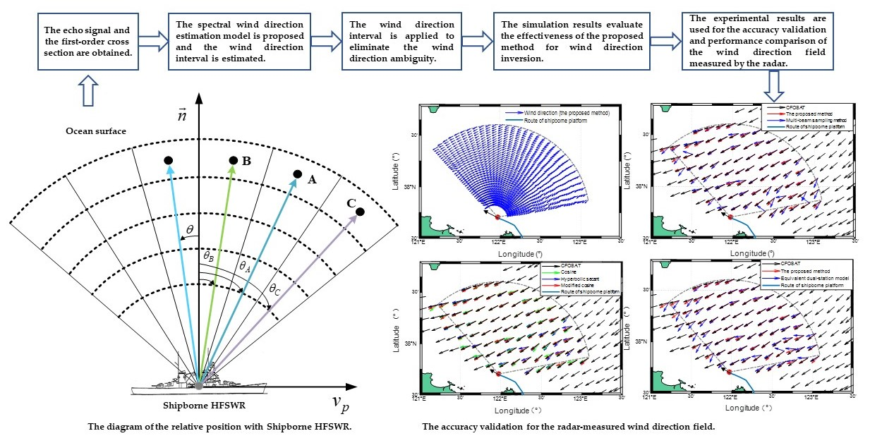
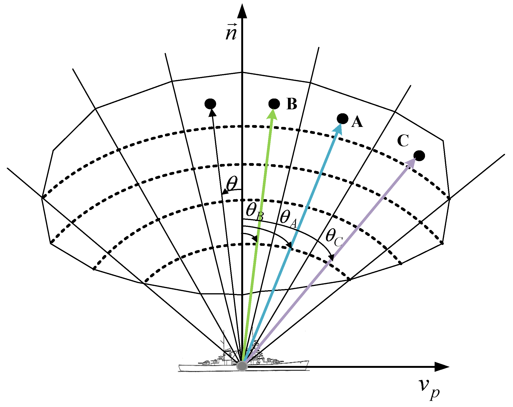
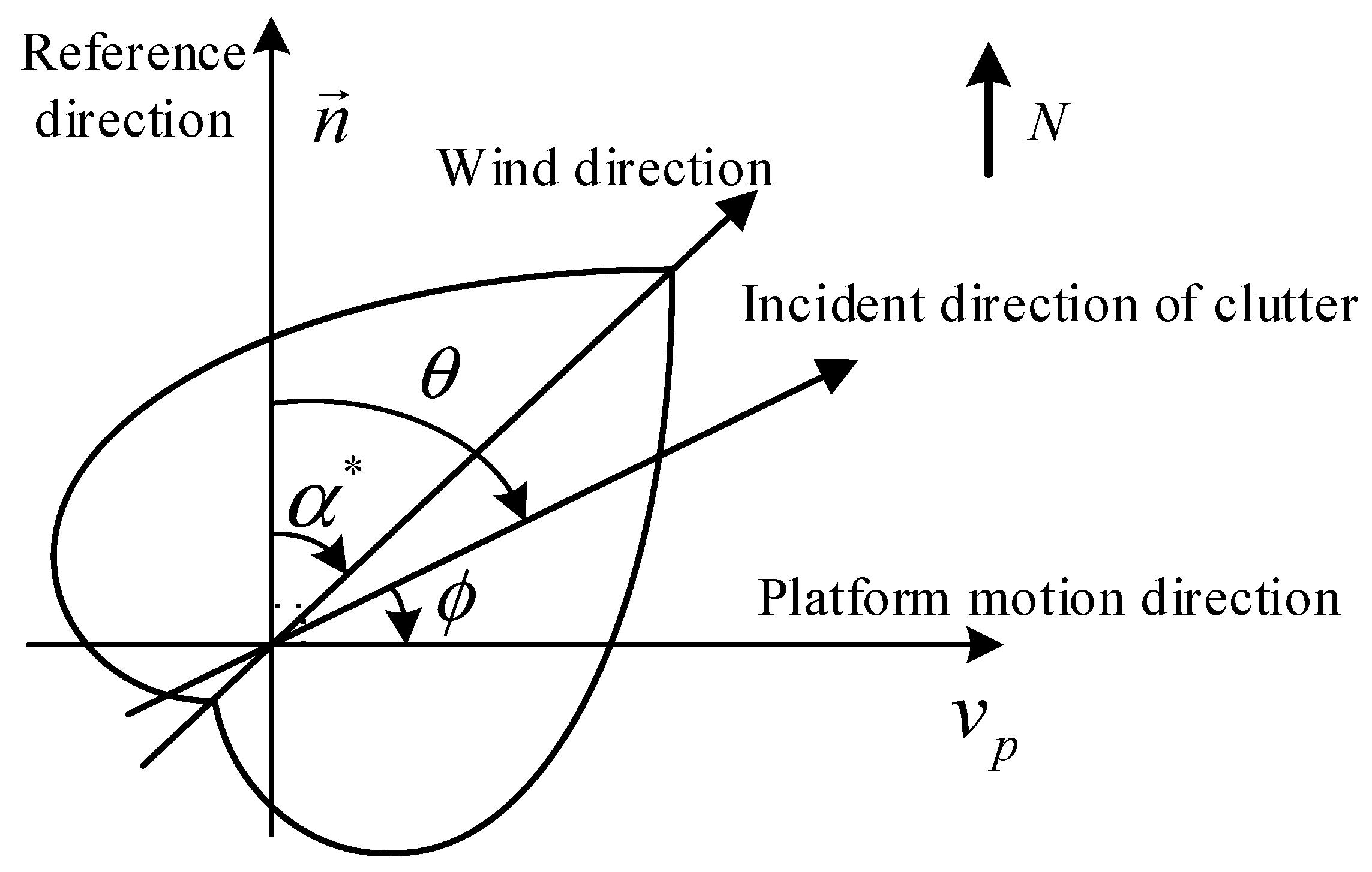
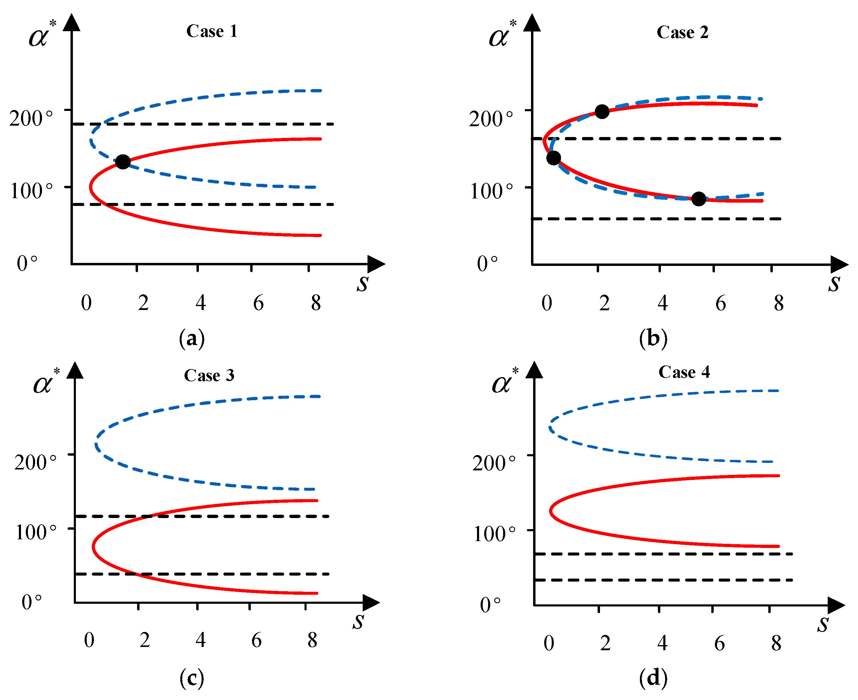
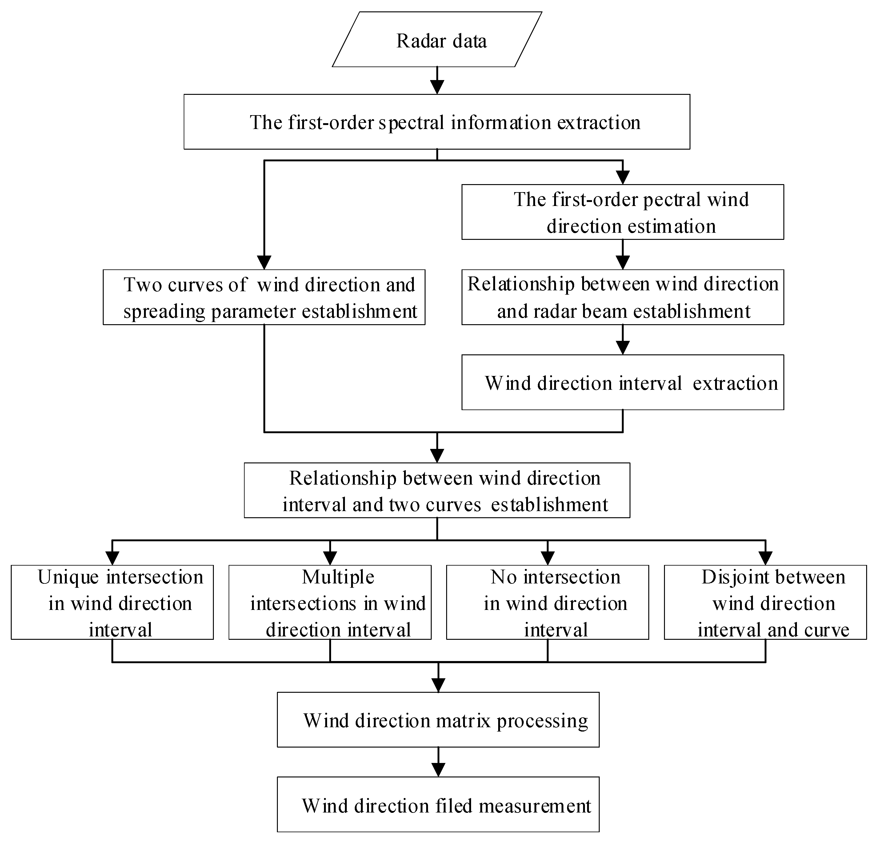
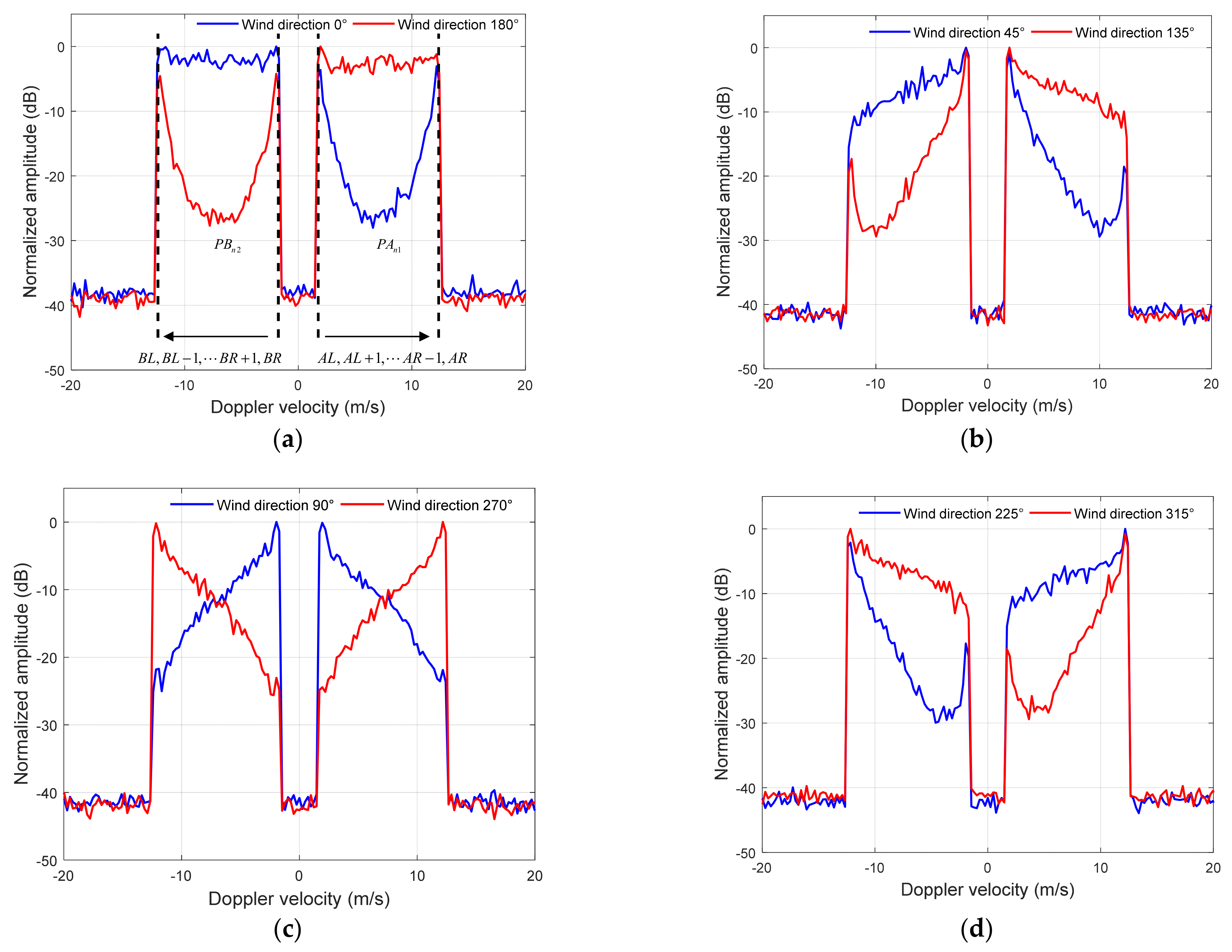
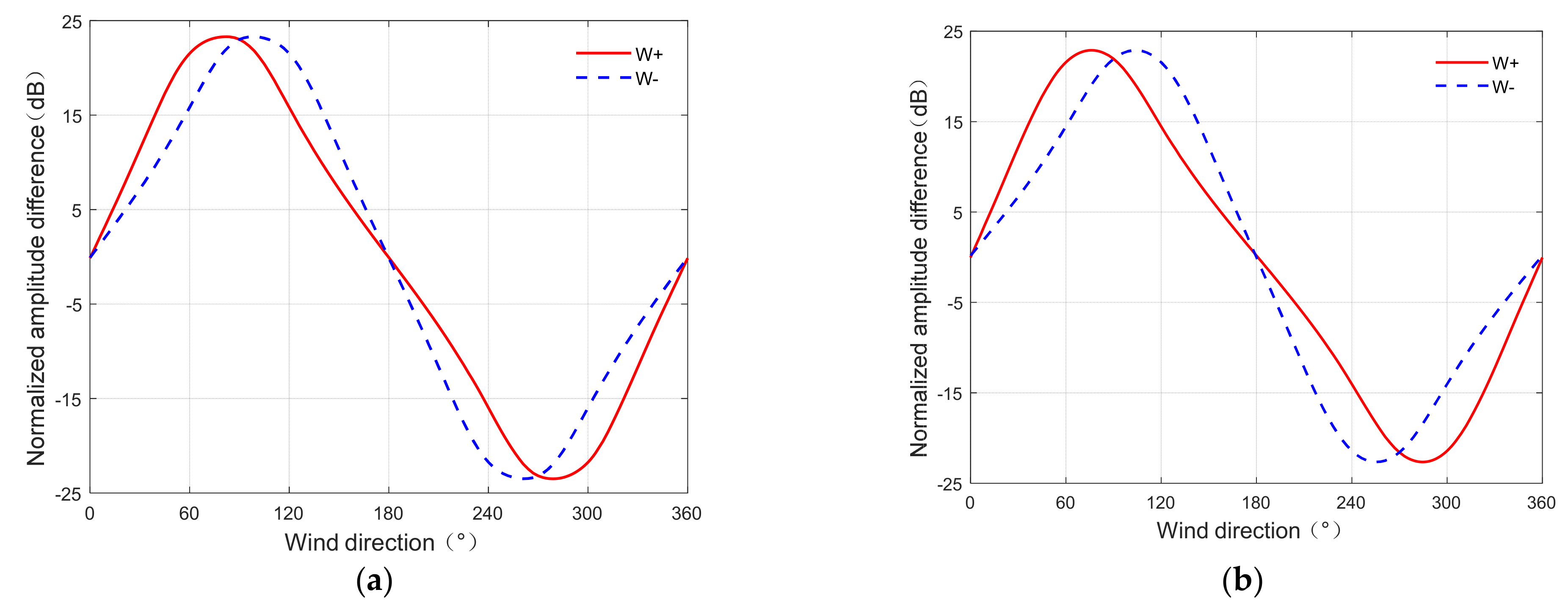
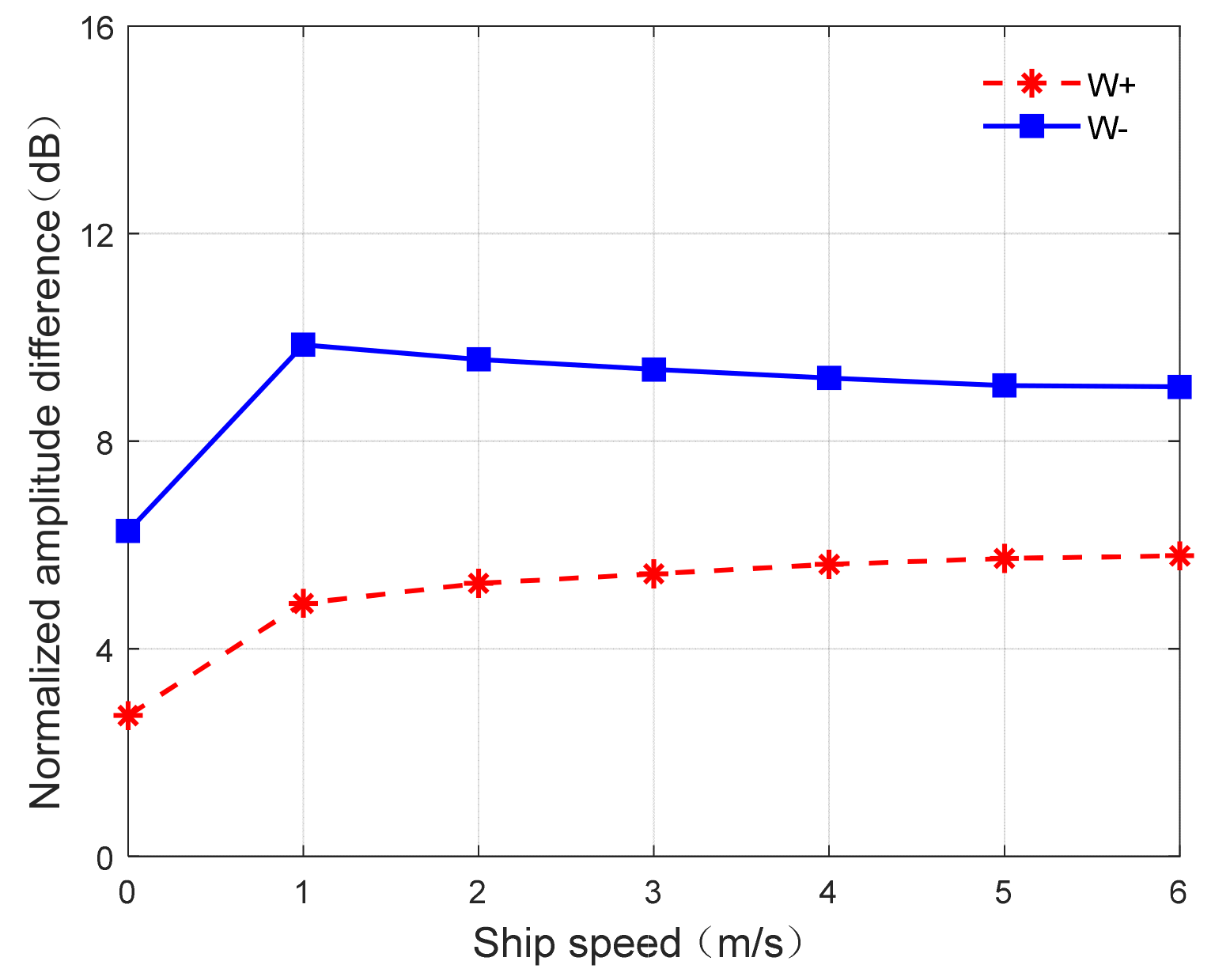
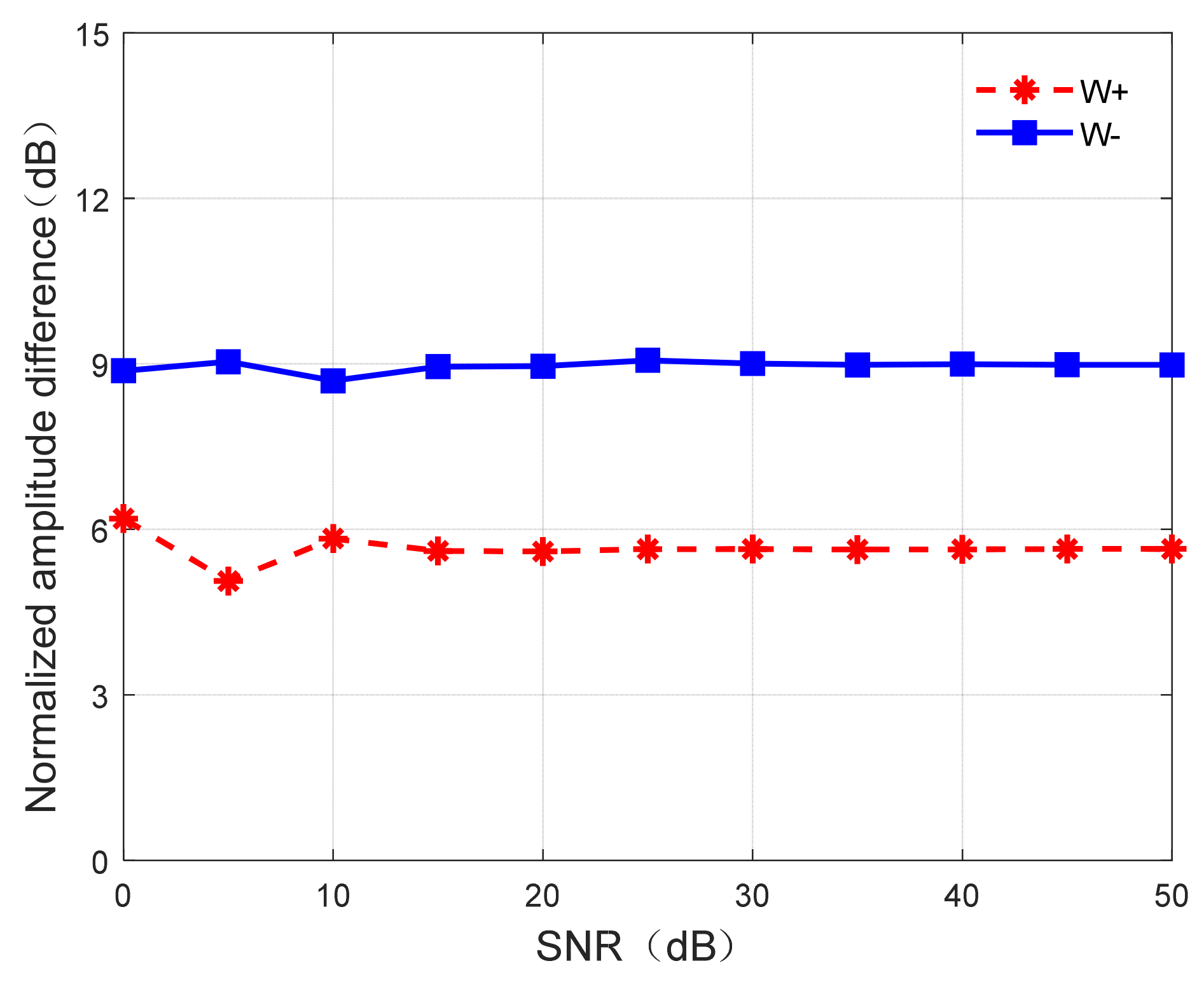
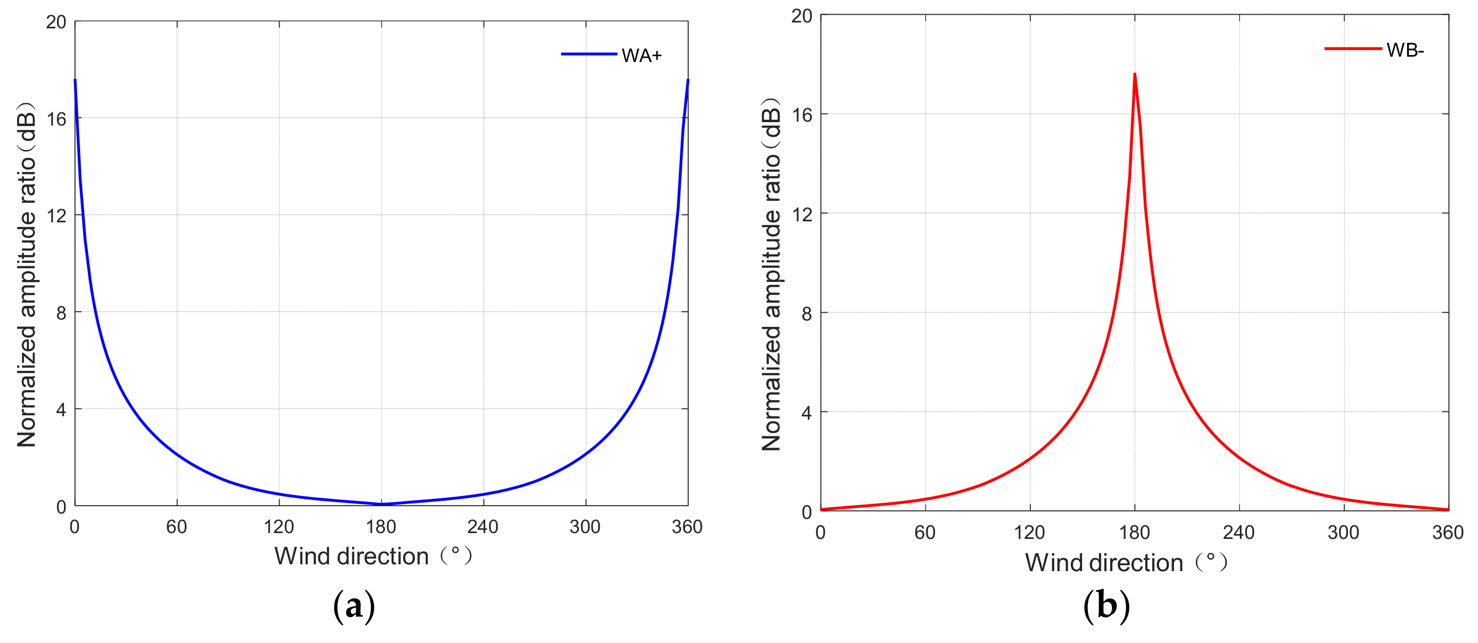
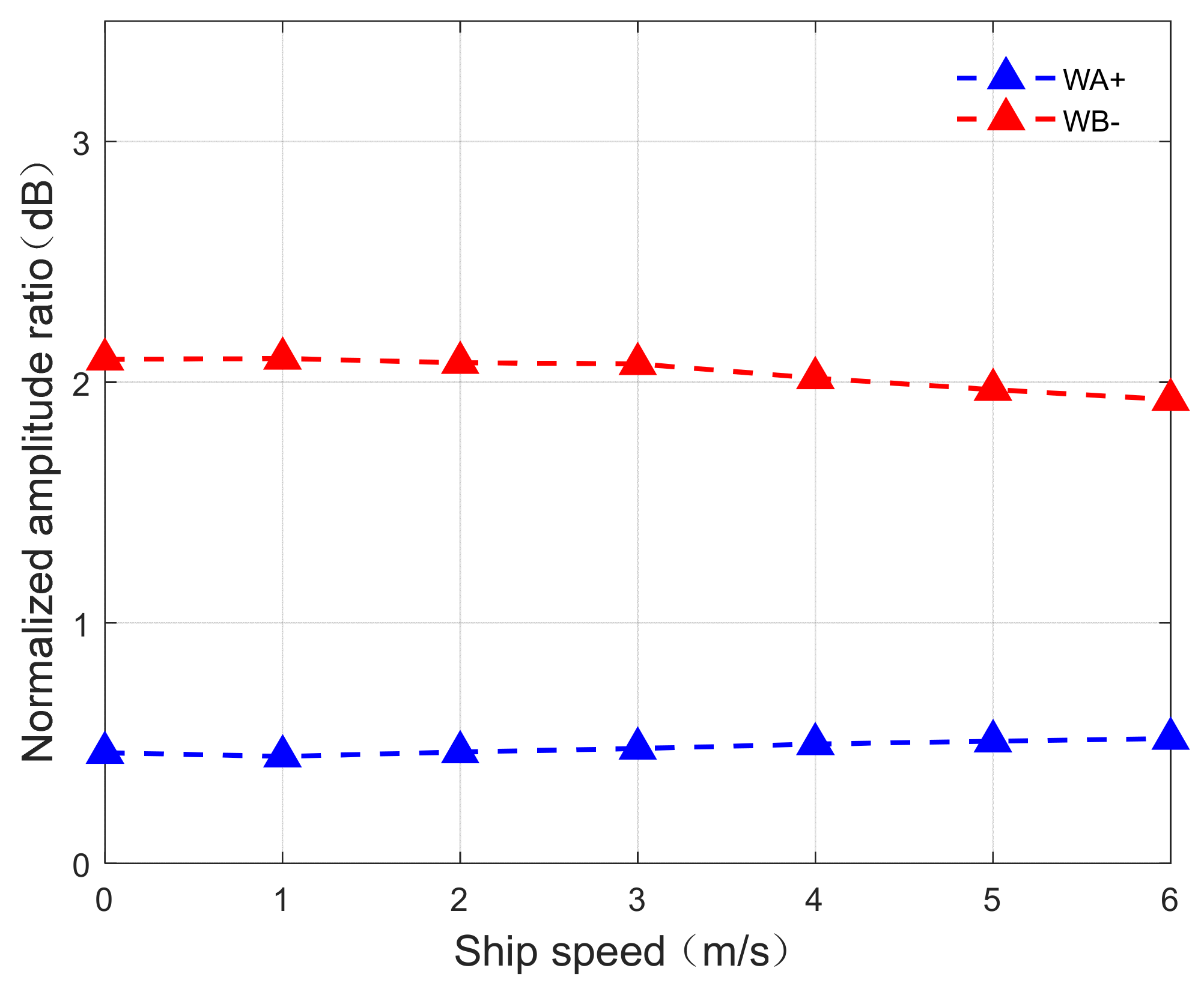
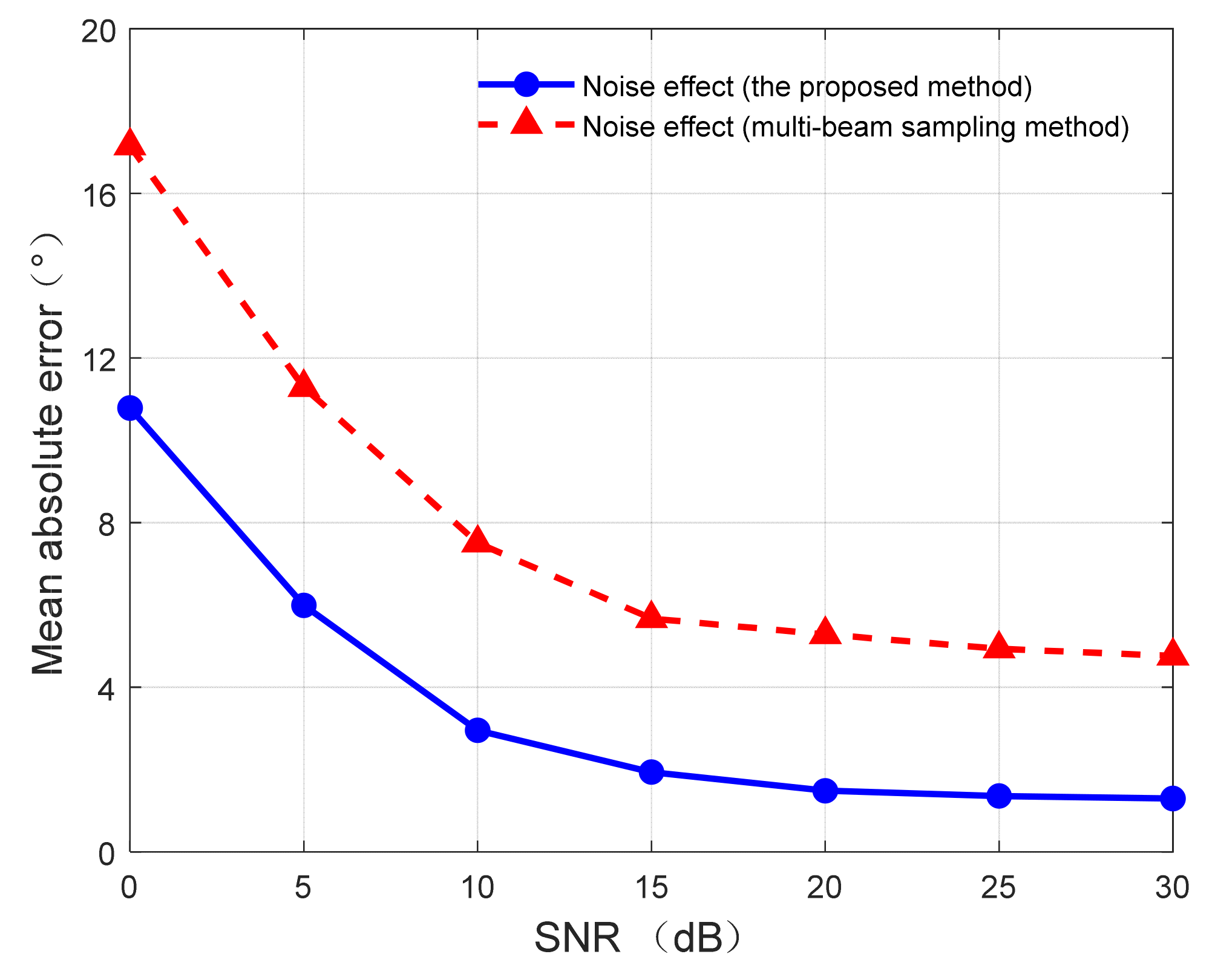
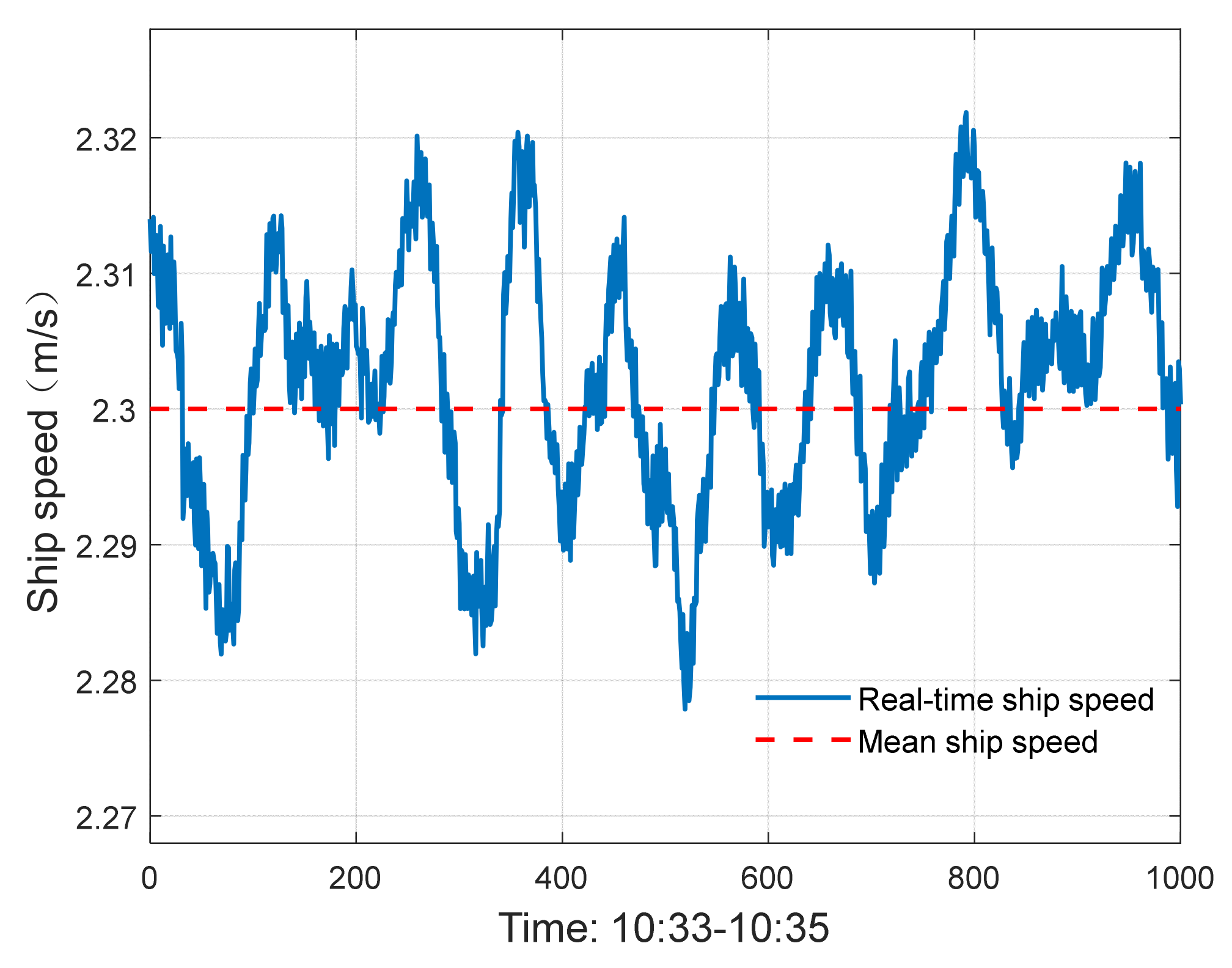
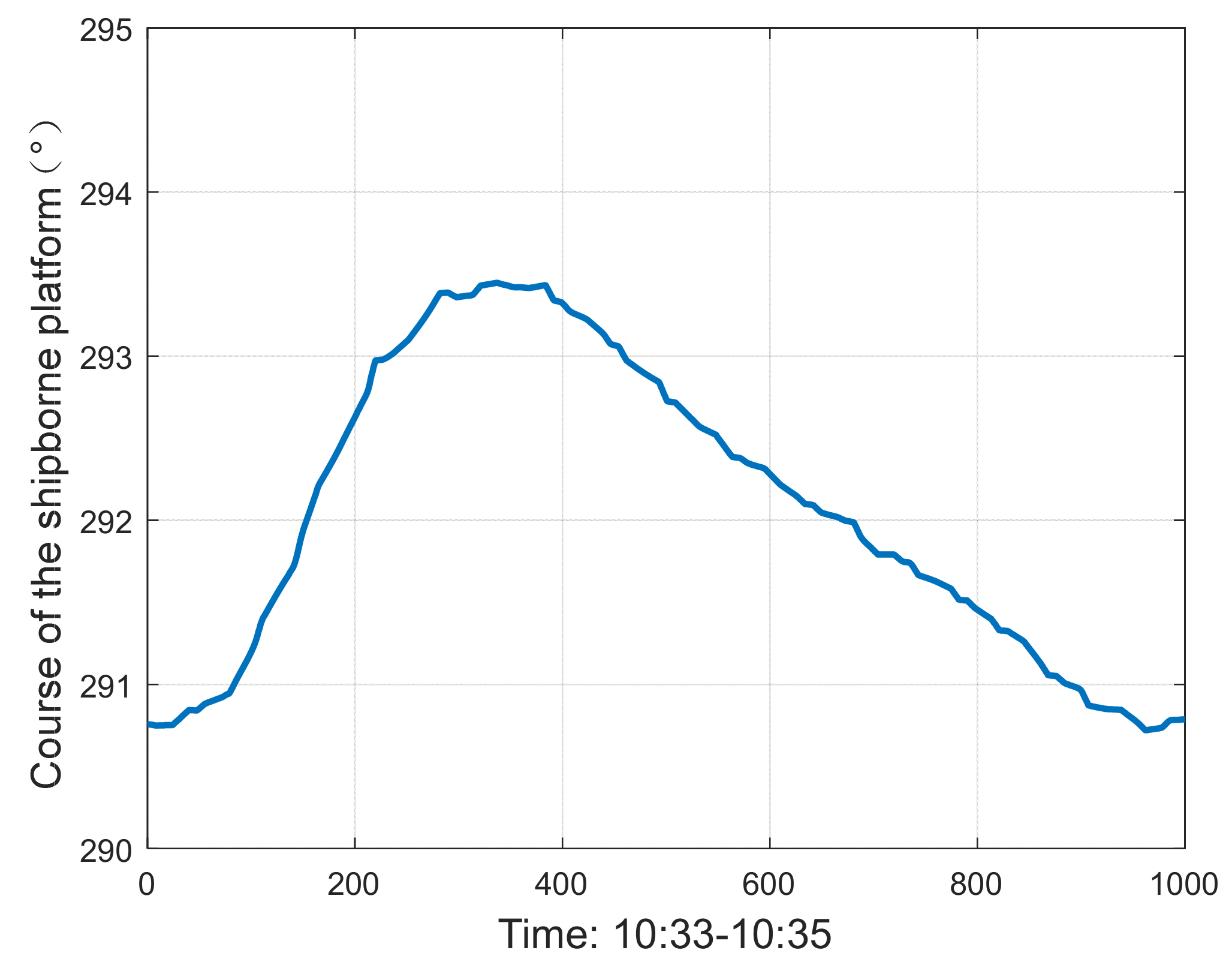
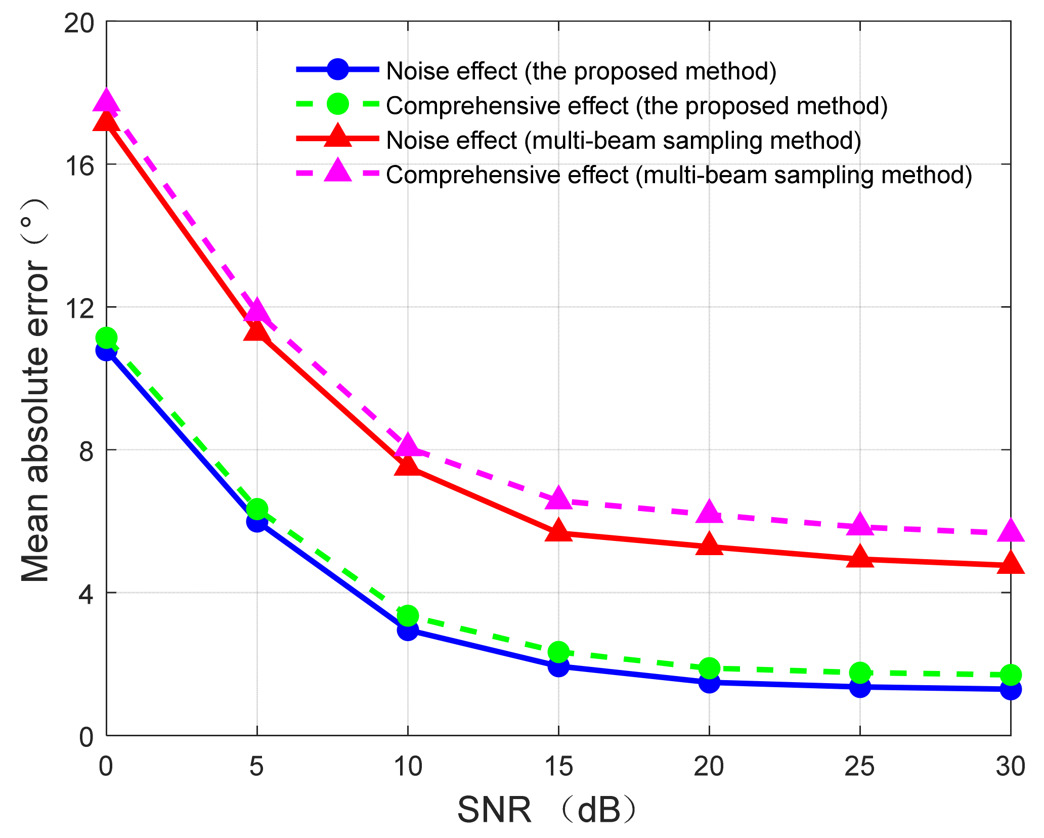
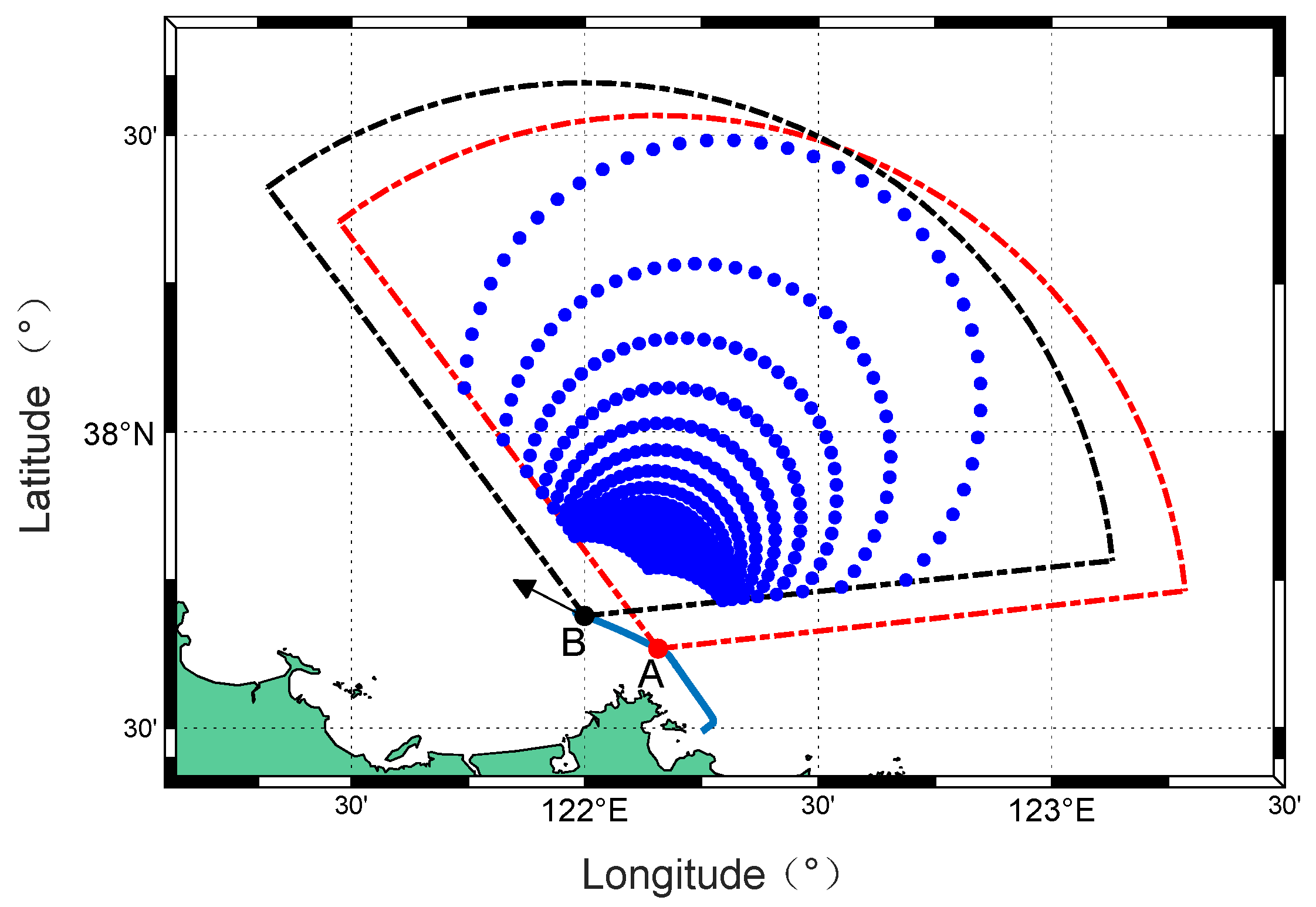
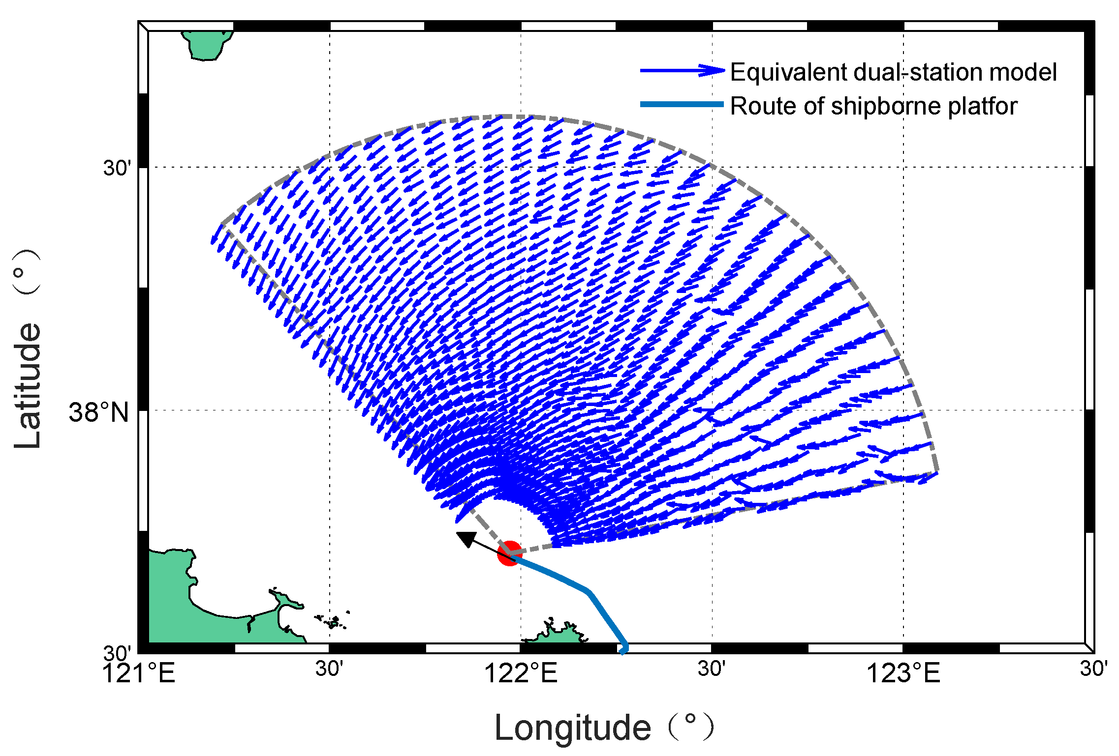
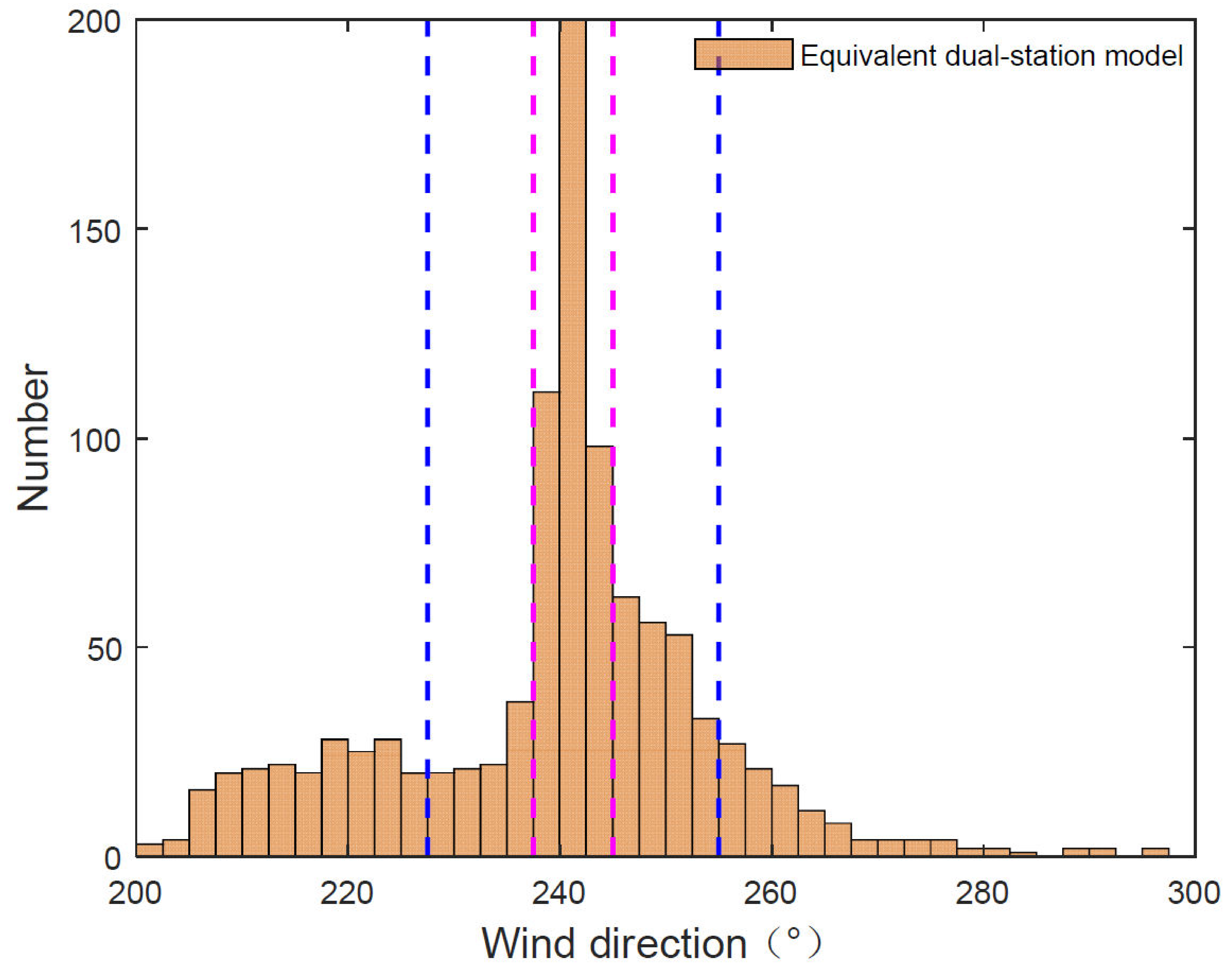
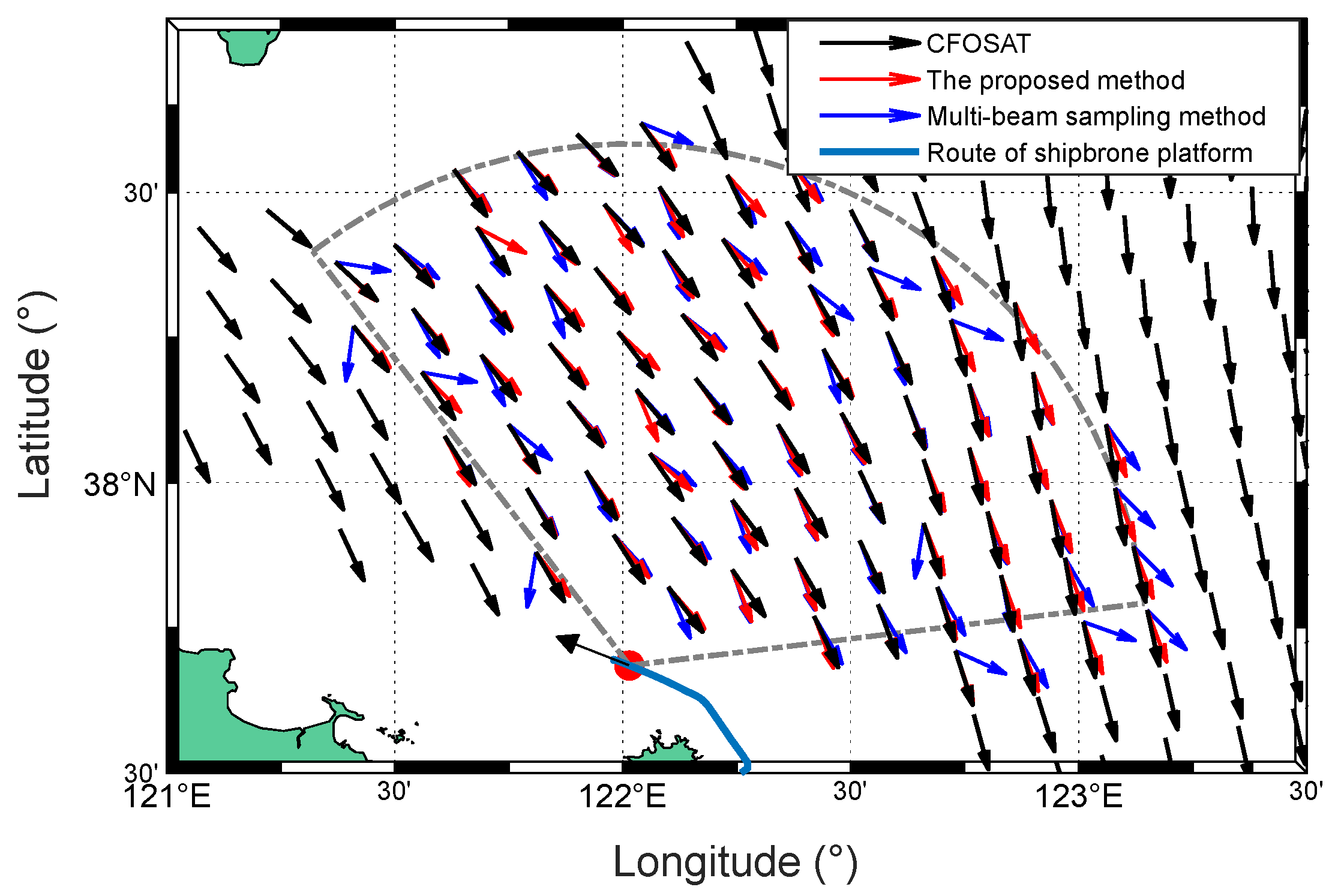
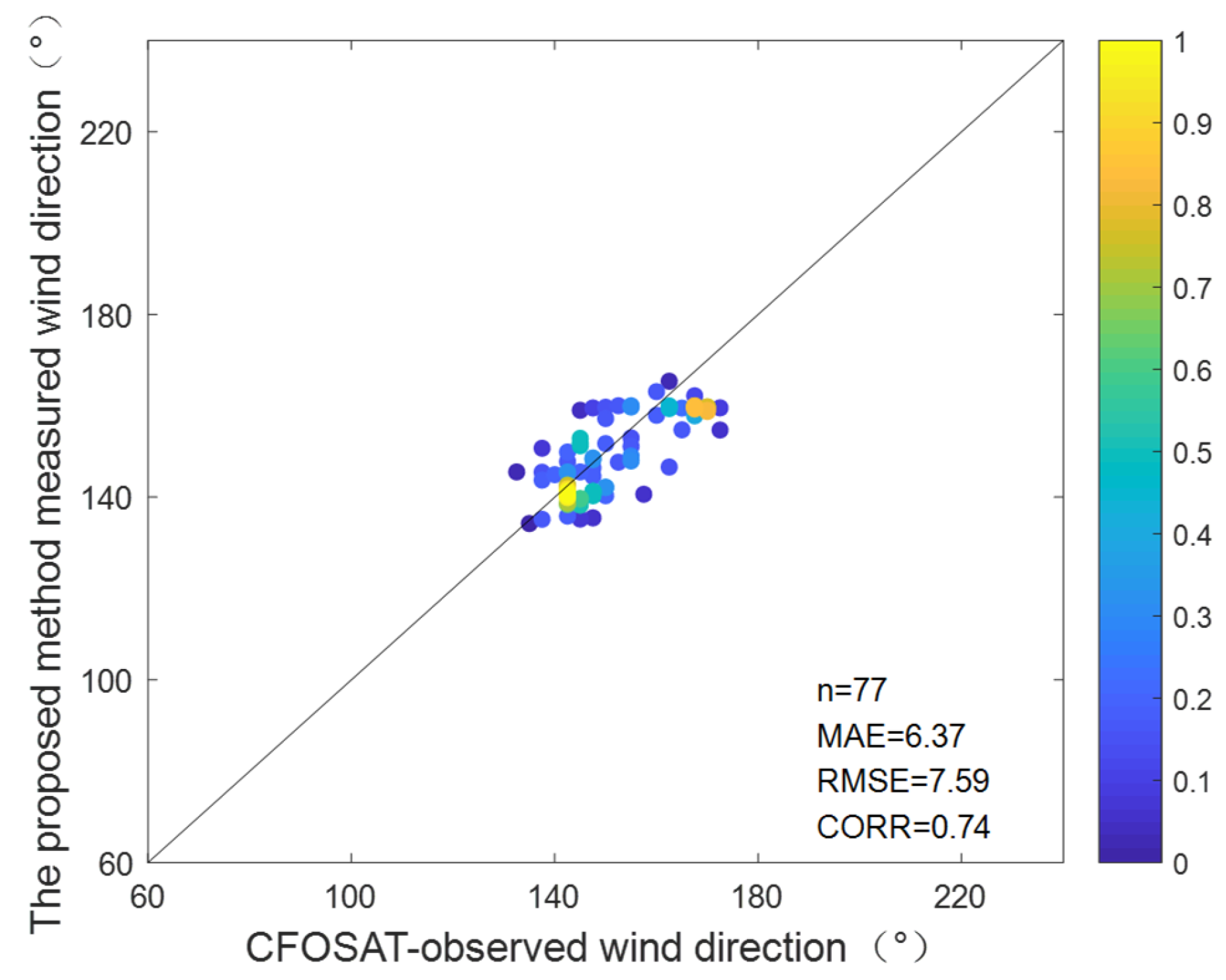
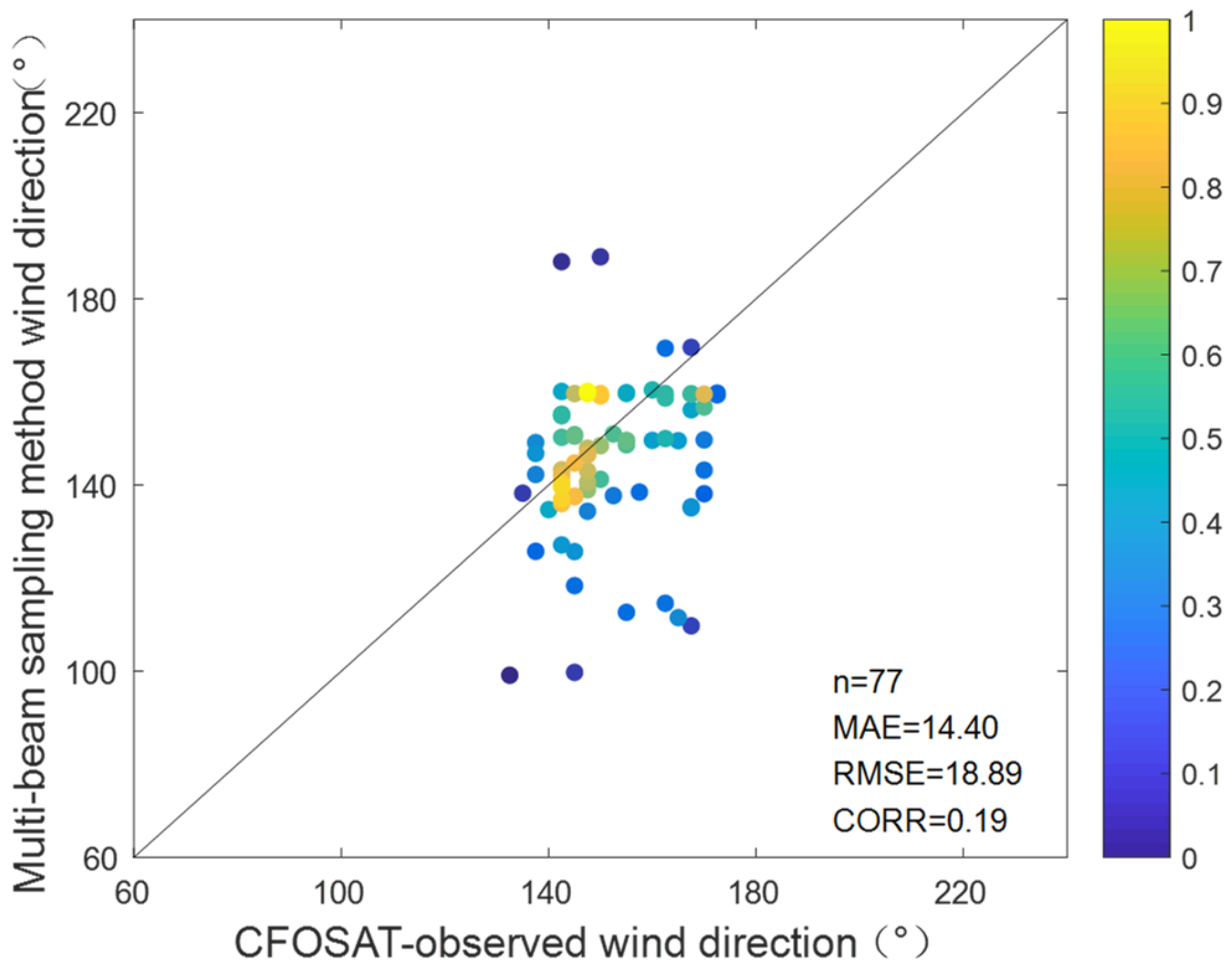
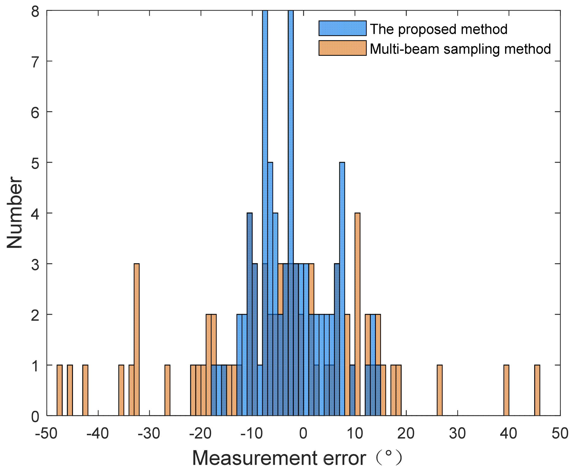
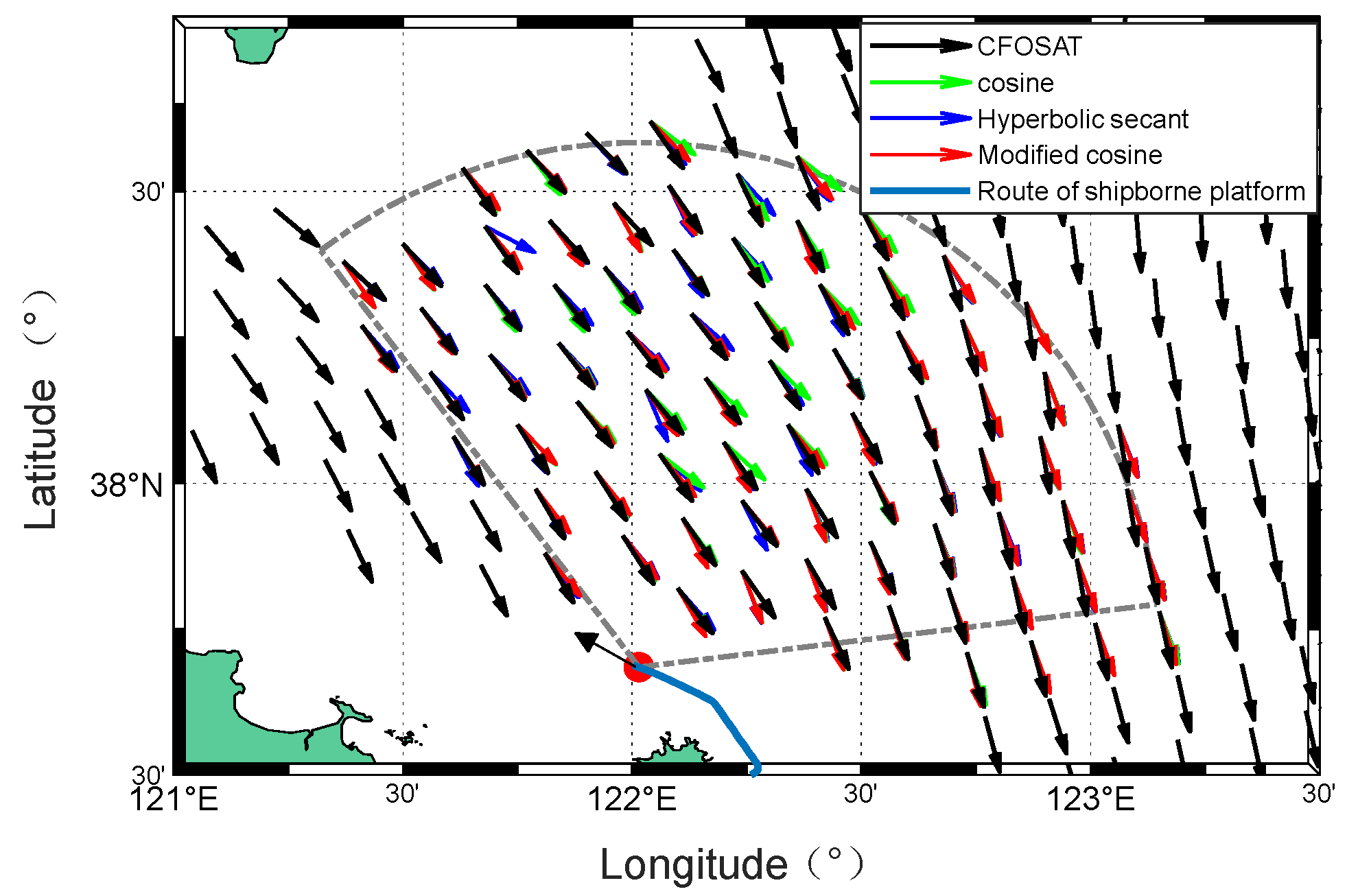
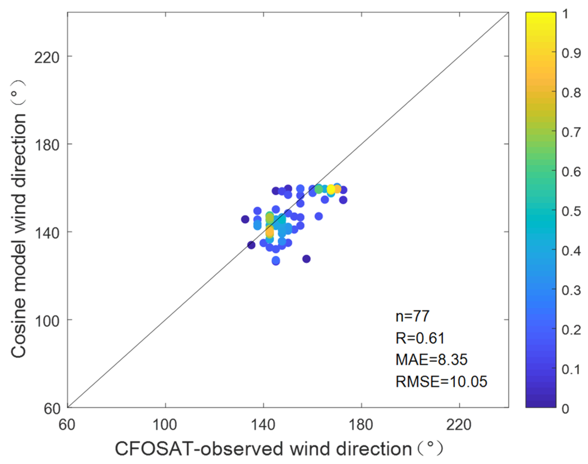
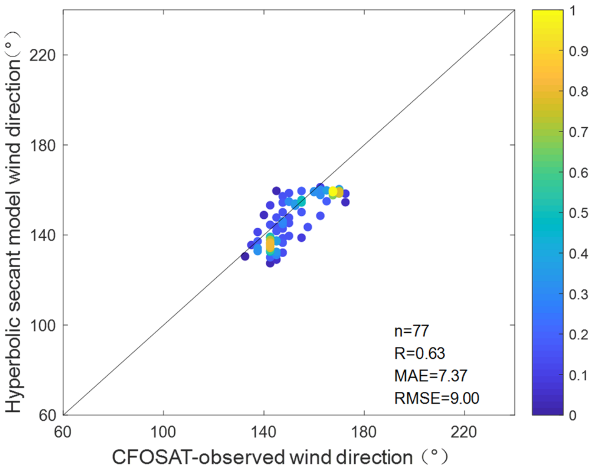
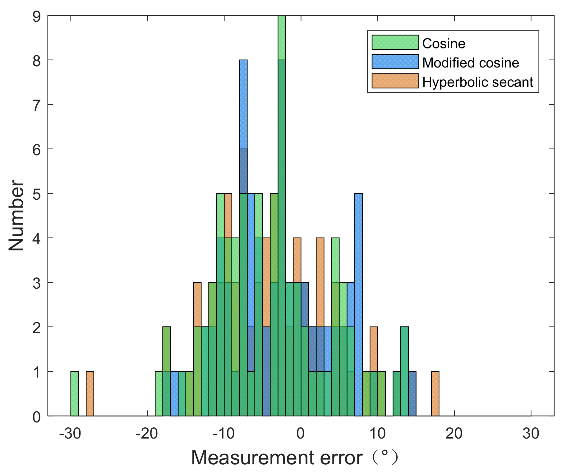
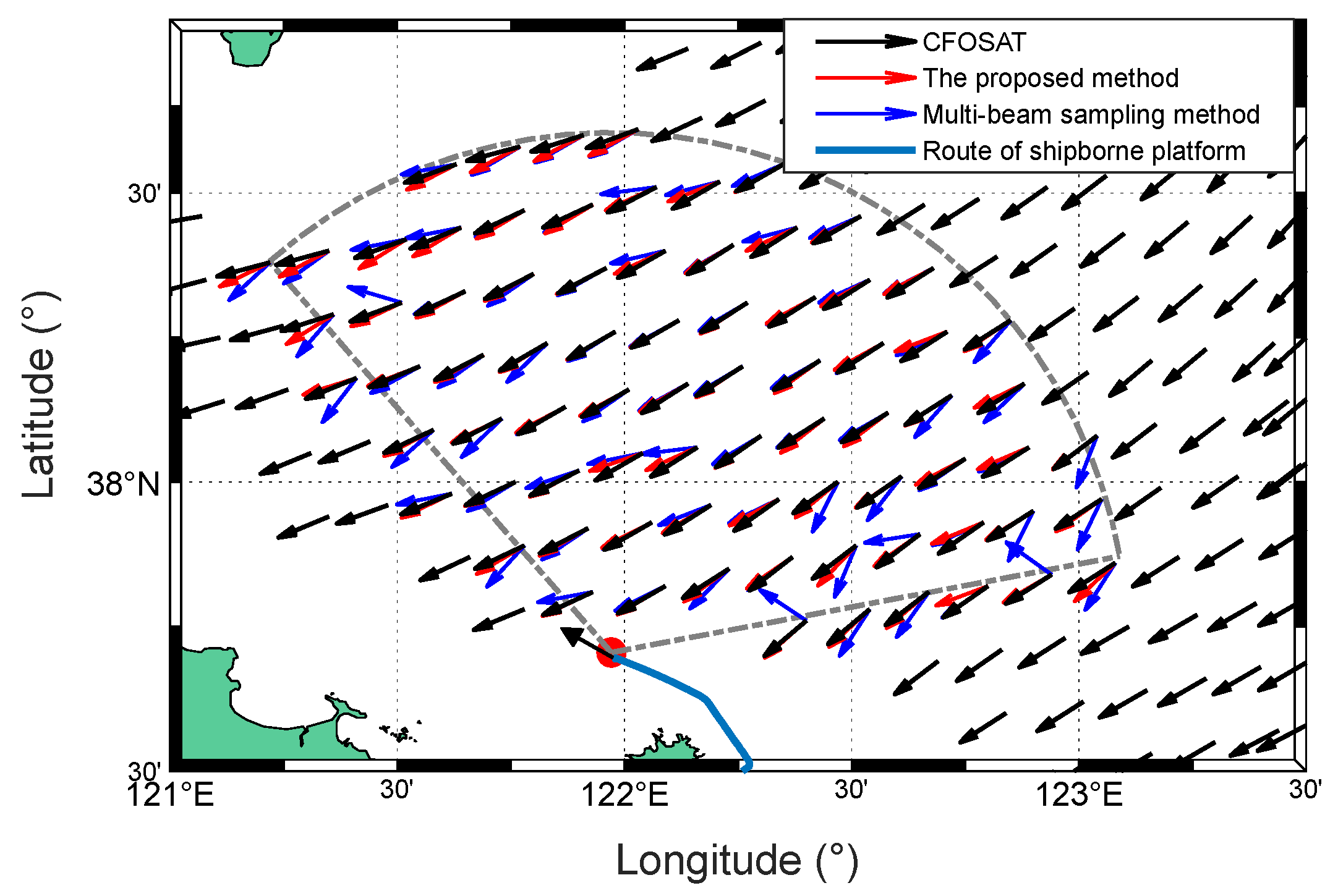
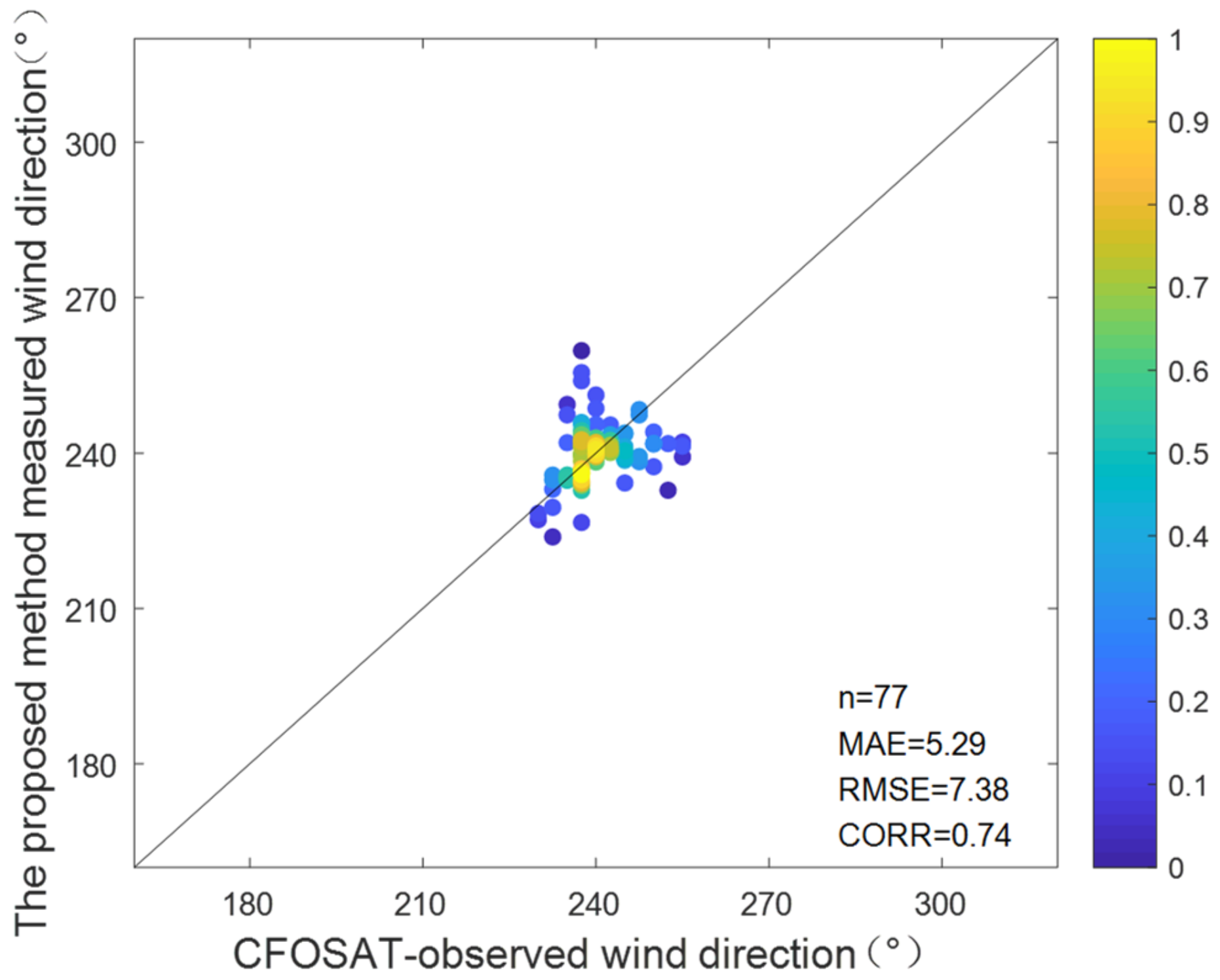
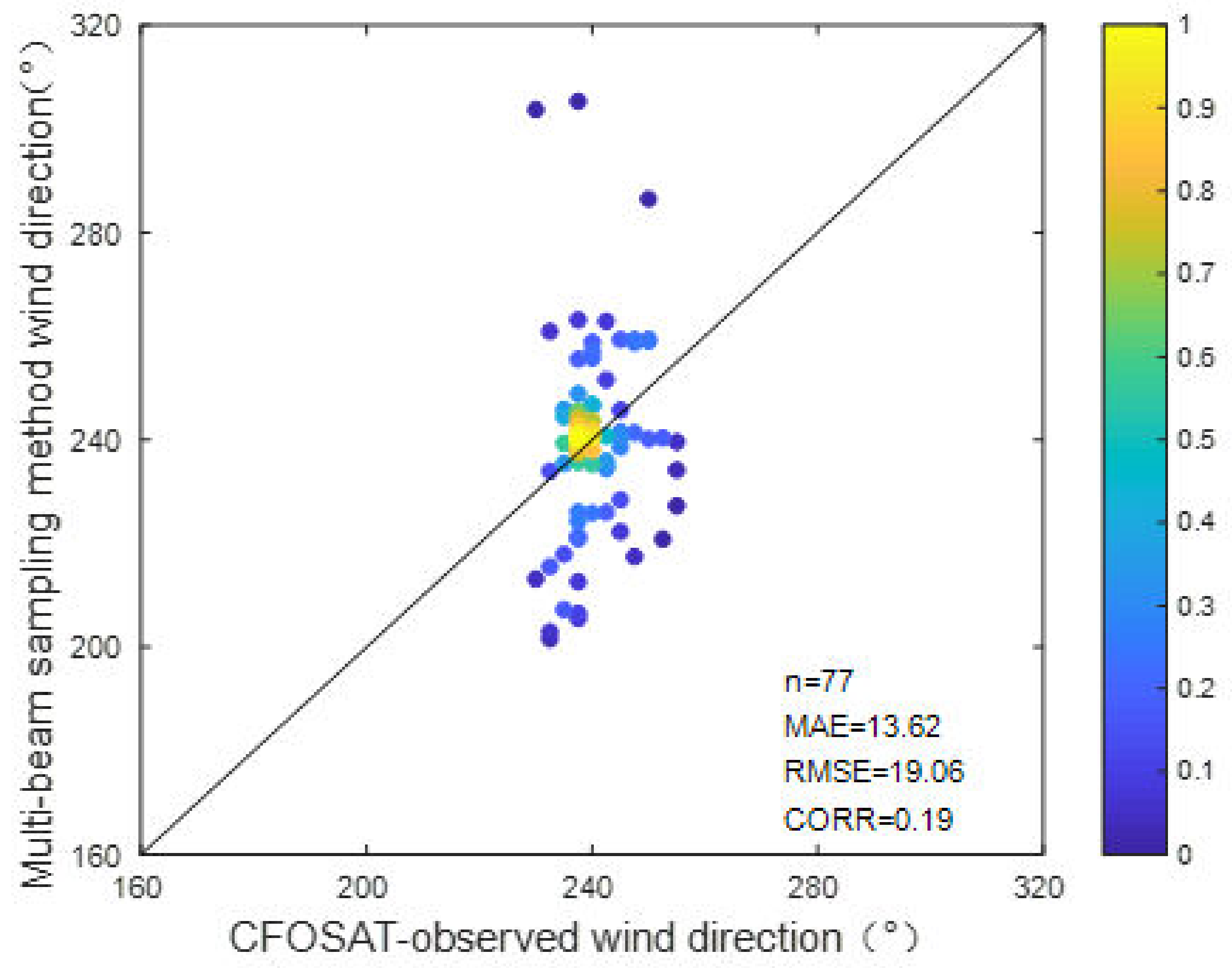
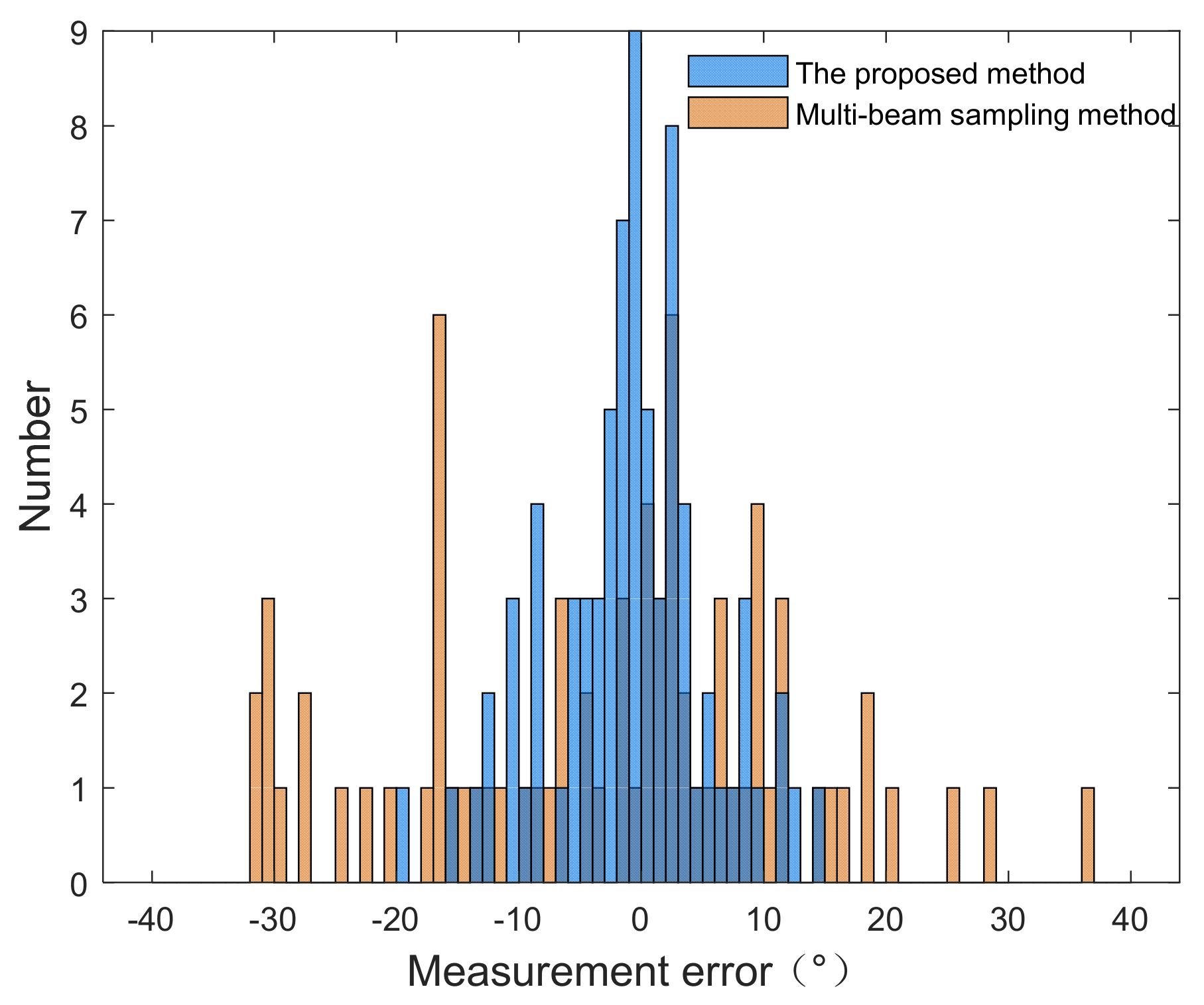
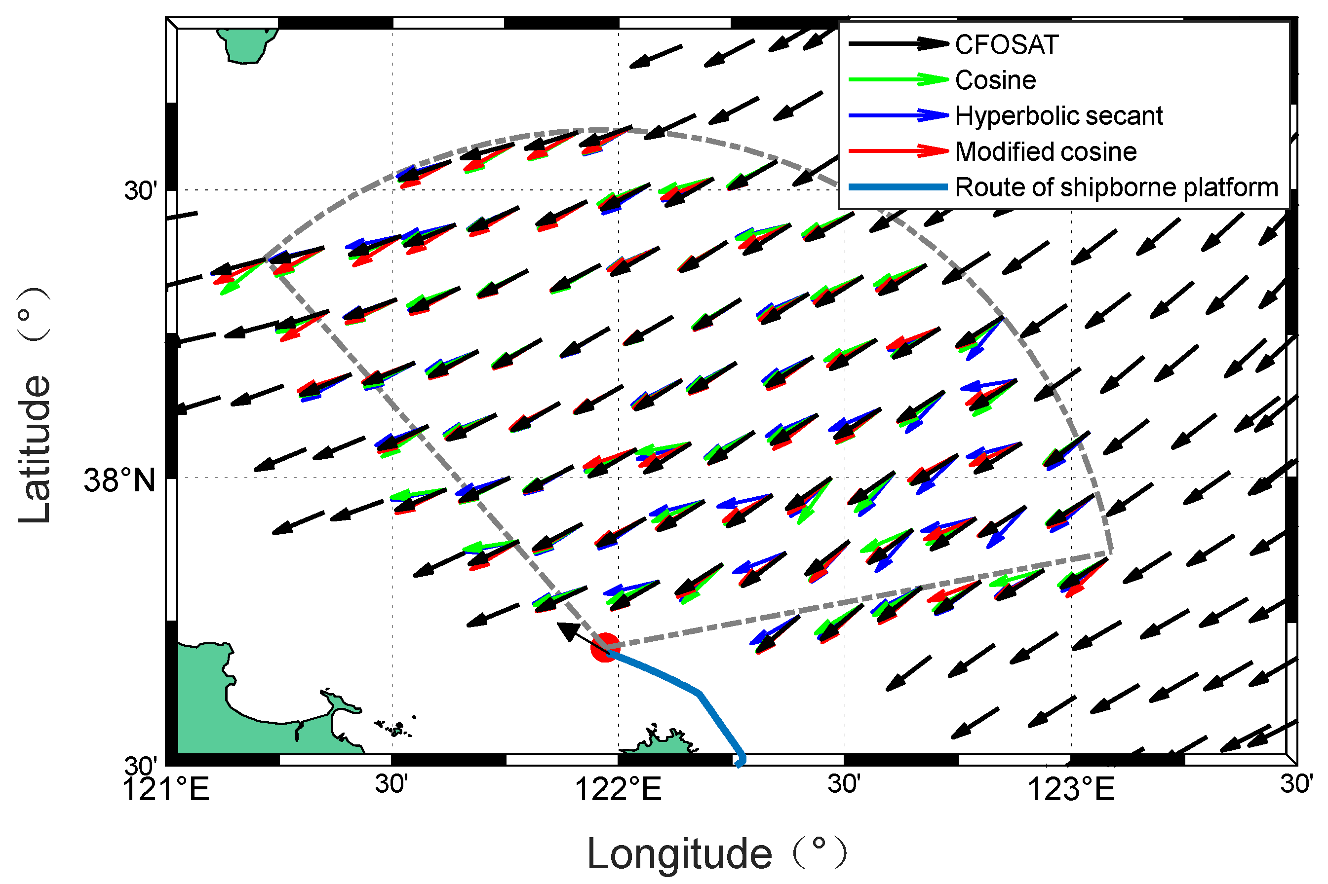
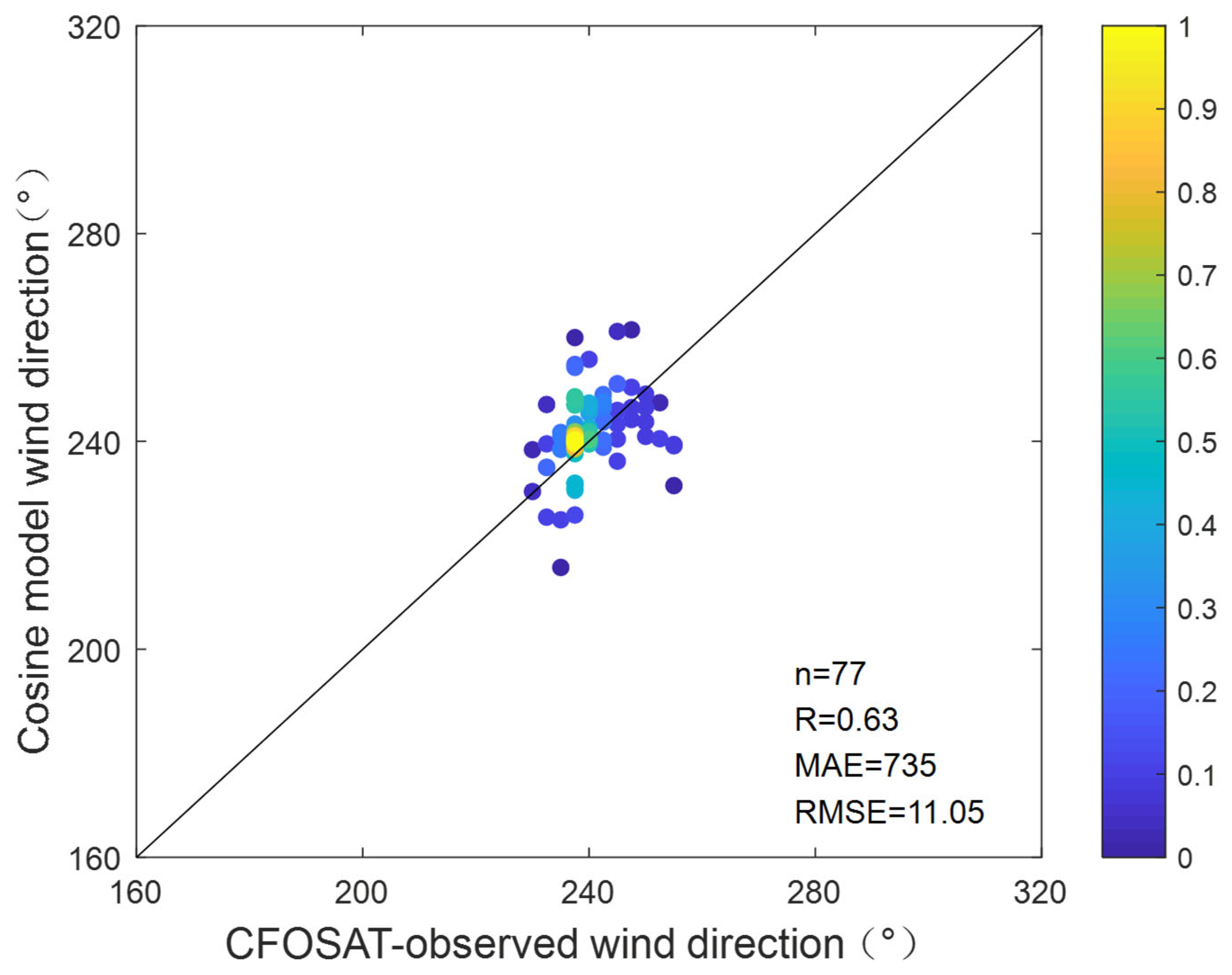
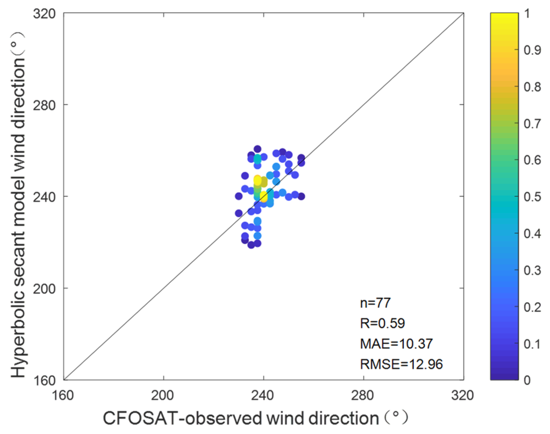
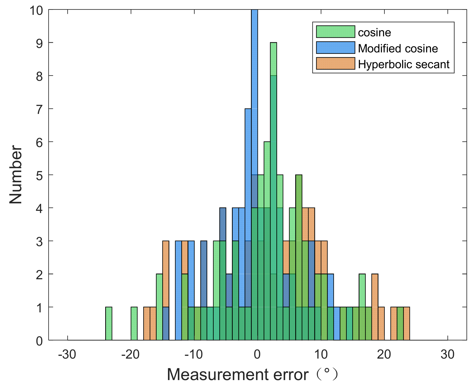
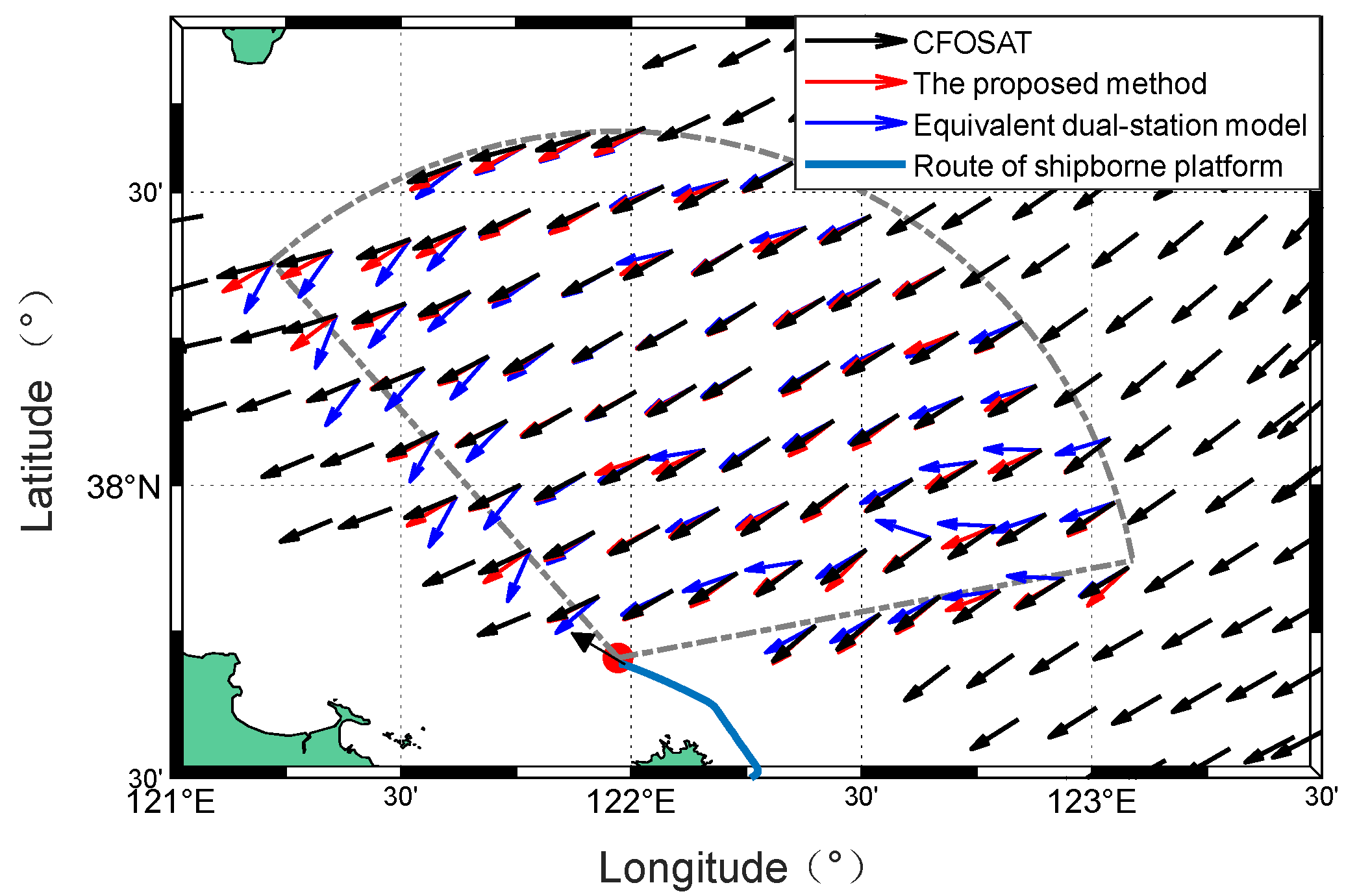
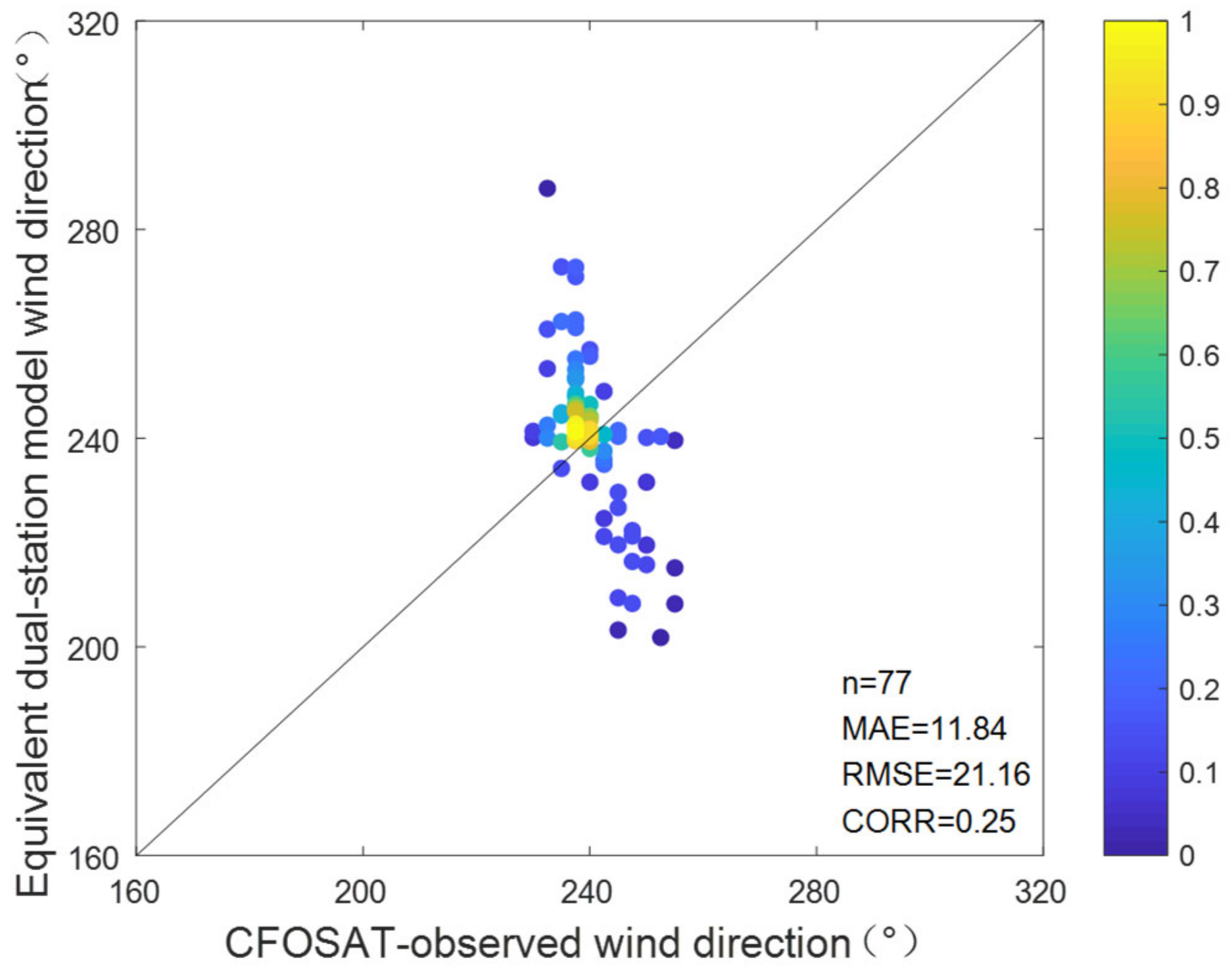
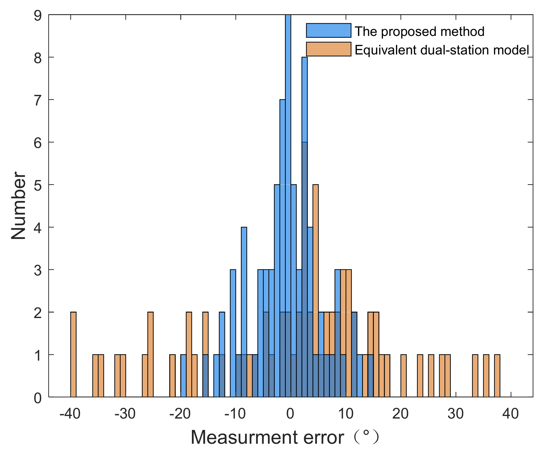
Table 1.
Statistical results of wind direction measurement.
| Item | The Proposed Method | The Multi-Beam Sampling Method |
|---|---|---|
| Percentage of wind direction error within −2°~2° | 56.76% | 22.23% |
| Mean absolute error | 1.97° | 9.26° |
| Standard deviation | 2.06° | 12.72° |
Table 2.
Radar operating parameters.
| Parameter | Parameter Value |
|---|---|
| Operating frequency (MHz) | 4.7 |
| Range resolution (km) | 2.5 |
| Bandwidth (kHz) | 60 |
| Coherent integration time (CIT) (s) | 128 |
| Number of transmitting antenna | 2 |
| Number of receiving antenna | 5 |
Table 3.
Normalized Doppler amplitude differences and ratios of boundary and broadened regions from experiment I.
Table 3.
Normalized Doppler amplitude differences and ratios of boundary and broadened regions from experiment I.
| Item | Batch 1 | Batch 2 | Batch 3 | Batch 4 | Batch 5 |
|---|---|---|---|---|---|
| (dB) | 5.31 | 5.28 | 5.35 | 5.41 | 5.31 |
| (dB) | 9.78 | 9.71 | 9.72 | 9.61 | 9.73 |
| (dB) | 0.19 | 0.18 | 0.19 | 0.20 | 0.18 |
| (dB) | 5.27 | 5.24 | 5.25 | 5.10 | 5.36 |
Table 4.
Statistical results of radar-measured wind direction using two methods in experiment I.
| Item | The Proposed Method (Modified Cosine Model) | The Multi-Beam Sampling Method |
|---|---|---|
| Percentage of wind directions within 155°~162.5° | 54.84% | 48.11% |
| Percentage of wind directions within 145°~172.5° | 78.44% | 67.92% |
| Mean wind direction | 155.53° | 158.22° |
| Standard deviation | 13.84° | 22.67° |
Table 5.
Statistical results of radar-measured wind direction using the two models from experiment I.
Table 5.
Statistical results of radar-measured wind direction using the two models from experiment I.
| Item | Cosine Model | Hyperbolic Secant Model |
|---|---|---|
| Percentage of wind directions within 155°~162.5° | 50.23% | 46.27% |
| Percentage of wind directions within 145°~172.5° | 73.82% | 77.79% |
| Mean wind direction | 156.07° | 153.55° |
| Standard deviation | 17.37° | 15.12° |
Table 6.
Normalized Doppler amplitude differences and ratios of boundary and broadened regions from experiment II.
Table 6.
Normalized Doppler amplitude differences and ratios of boundary and broadened regions from experiment II.
| Item | Batch 1 | Batch 2 | Batch 3 | Batch 4 | Batch 5 |
|---|---|---|---|---|---|
| (dB) | −14.10 | −14.02 | −14.04 | −14.12 | −14.07 |
| (dB) | −21.42 | −21.43 | −21.43 | −21.42 | −21.43 |
| (dB) | 0.47 | 0.46 | 0.47 | 0.49 | 0.44 |
| (dB) | 2.14 | 2.14 | 2.14 | 2.20 | 2.13 |
Table 7.
Statistical results of radar-measured wind direction using the two methods ffrom experiment II.
Table 7.
Statistical results of radar-measured wind direction using the two methods ffrom experiment II.
| Item | The Proposed Method (Modified Cosine Model) | The Multi-Beam Sampling Method |
|---|---|---|
| Percentage of wind directions within 237.50°~245° | 43.13% | 40.10% |
| Percentage of wind directions within 227.50°~255° | 74.47% | 67.74% |
| Mean wind direction | 239.65° | 243.38° |
| Standard deviation | 13.45° | 19.71° |
Table 8.
Statistical results of radar-measured wind direction using the two models from experiment II.
Table 8.
Statistical results of radar-measured wind direction using the two models from experiment II.
| Item | Cosine Model | Hyperbolic Secant Model |
|---|---|---|
| Percentage of wind directions within 237.50°~245° | 37.51% | 40.28% |
| Percentage of wind directions within 227.50°~255° | 70.51% | 74.97% |
| Mean wind direction | 242.13° | 247.60° |
| Standard deviation | 15.74° | 17.38° |
Table 9.
Statistical results of radar-measured wind direction using the two methods from experiment III.
Table 9.
Statistical results of radar-measured wind direction using the two methods from experiment III.
| Item | The Proposed Method | The Equivalent Dual-Station Model |
|---|---|---|
| Percentage of wind directions within 237.50°~245° | 43.13% | 39.33% |
| Percentage of wind directions within 227.50°~255° | 74.47% | 62.67% |
| Mean wind direction | 239.65° | 237.51° |
| Standard deviation | 13.45° | 19.71° |
Disclaimer/Publisher’s Note: The statements, opinions and data contained in all publications are solely those of the individual author(s) and contributor(s) and not of MDPI and/or the editor(s). MDPI and/or the editor(s) disclaim responsibility for any injury to people or property resulting from any ideas, methods, instructions or products referred to in the content. |
© 2023 by the authors. Licensee MDPI, Basel, Switzerland. This article is an open access article distributed under the terms and conditions of the Creative Commons Attribution (CC BY) license (https://creativecommons.org/licenses/by/4.0/).
Share and Cite
MDPI and ACS Style
Zhang, Y.; Wang, Y.; Ji, Y.; Li, M. Unambiguous Wind Direction Estimation Method for Shipborne HFSWR Based on Wind Direction Interval Limitation. Remote Sens. 2023, 15, 2952. https://doi.org/10.3390/rs15112952
AMA Style
Zhang Y, Wang Y, Ji Y, Li M. Unambiguous Wind Direction Estimation Method for Shipborne HFSWR Based on Wind Direction Interval Limitation. Remote Sensing. 2023; 15(11):2952. https://doi.org/10.3390/rs15112952
Chicago/Turabian StyleZhang, Yunfeng, Yiming Wang, Yonggang Ji, and Ming Li. 2023. "Unambiguous Wind Direction Estimation Method for Shipborne HFSWR Based on Wind Direction Interval Limitation" Remote Sensing 15, no. 11: 2952. https://doi.org/10.3390/rs15112952
Note that from the first issue of 2016, this journal uses article numbers instead of page numbers. See further details here.