
Analysis of East Asia Wind Vectors Using Space–Time Cross-Covariance Models

1
Department of Mathematics, Hanyang University, Seoul 04763, Republic of Korea
2
Research Institute for Natural Sciences, Hanyang University, Seoul 04763, Republic of Korea
3
Division of Statistics and Data Science, University of Cincinnati, Cincinnati, OH 45221, USA
*
Author to whom correspondence should be addressed.
Remote Sens. 2023, 15(11), 2860; https://doi.org/10.3390/rs15112860
Submission received: 21 April 2023
/
Revised: 26 May 2023
/
Accepted: 29 May 2023
/
Published: 31 May 2023
(This article belongs to the Special Issue Spatial and Spatio-Temporal Statistics: Methods and Applications in Remote Sensing)
Abstract
:As the risk posed by climate change becomes increasingly evident, countries across the world are constantly seeking alternative energy sources. Wind energy has substantial potential for future energy portfolios without having negative impacts on the environment. In developing nationwide and worldwide energy plans, understanding the spatio-temporal pattern of wind is crucial. We analyze wind vectors in the region of East Asia from the fifth-generation ECMWF atmospheric reanalysis. To model the wind vectors, we consider Tukey g-and-h transformation-based non-Gaussian processes, along with multivariate covariance functions. The proposed model can address non-Gaussian features and nonstationary dependence structures of wind vectors. In addition, a two-step inference scheme coupled with the composite likelihood method is applied to handle the computational issues posed by a large dataset. In the first step, we fit the temporal dependence structures of data with a location-specific non-Gaussian time series model. This allows us to remove substantial amounts of nonstationary variations in both space and time, and thus, relatively simple covariance models can handle large and complicated data in the second step. We show that the proposed method with a covariance structure reflecting the nonstationarity due to the latitude difference and the land–ocean difference leads to better predictions for wind speed as well as wind potential, which is crucial for planning wind power generation.
1. Introduction
As many countries are becoming increasingly interested in seeking alternative energy sources, the popularity of wind power or wind energy is becoming more prominent [1,2]. Because wind is a clean and renewable energy source with no critically negative impacts on the environment, it has the apparent potential to contribute to the future energy portfolio. Moreover, unlike coal, natural gas, or oil, the wind does not result in greenhouse gas emissions when it generates electricity and can mitigate the influence of anthropogenic greenhouse gases on global warming [3]. As a result, it is one of the fastest-growing sources of electricity production globally [4].
To better understand the behavior of wind data and its energy evaluation, climate reanalysis provides a valuable tool that is a numerical illustration of the recent climate using models coupled with observations [5]. Climate reanalysis can be used for various climate studies and numerical weather predictions, and thus, it can help to understand the pace of climate change, such as global warming. Furthermore, the reanalysis data cover large portions of the Earth and its atmosphere, so they can help provide climate and weather assessment in countries where available regional studies are sparse. The simulation-based climate model output and reanalysis data often involve large datasets, and there have been various works on statistically analyzing the wind patterns from climate simulations and real-world observations in the literature. For example, Jeong et al. [6,7] studied global wind speed data from publicly available simulations, and they proposed a method to create surrogates of the original wind datasets. Tagle et al. [8] considered a smaller region from the same simulations to reduce the amount of computation and analyzed the daily wind speeds based on a non-Gaussian model (with a multivariate skew-t distribution). In their regional simulation, Chen et al. [9] analyzed future estimates of wind potential in Saudi Arabia and concluded the energy potential over western regions will persist until the middle of the 21st century. Wind energy resources from weather simulations of the region, coupled with a high-resolution, were assessed using the skew-t distribution [10]. These authors found that more abundant wind resources exist over many areas in Saudi Arabia than the estimates proposed in the previous studies based on coarser resolution datasets. Another important thread of wind-related research is on finding optimal locations of wind farms and the extrapolation of wind speed at a certain height (relating to the hub height of the wind turbine). Several works have been conducted on this problem, e.g., optimal wind farm location [11] and speed exploration [12], and we refer to [13] for a comprehensive review on the literature over the most recent 40 years (1978–2018). As described in the “Renewable Energy 2030 Plan”, the Korean government is interested in finding optimal regions for wind farms to expand their current wind power capacity [14], and hence, a similar analysis will be useful for future planning.
For wind data, statistical modeling approaches based on stochastic processes and covariance functions are popular. As examples of the statistical modeling of wind fields, Cripps et al. [15] proposed a statistical model to analyze and forecast surface-level wind. A Bayesian hierarchical model was introduced to handle spatio-temporal processes, and they demonstrated the effectiveness of forecasting one day in advance for wind fields near Sydney Harbour. Ailliot et al. [16] studied the space–time variations of wind fields using the Markov-switching autoregressive model. Nonstationarity in wind dynamics was also considered via the regime-switching approach for forecasting [17]. Recently, a neural-network-based model was proposed to handle nonlinear dynamics of hourly wind [18]. This work helped close the gap between machine learning techniques and spatio-temporal statistics. Some other wind energy applications based on statistical models can be found in [19], such as wind turbine performance analysis and production efficiency analysis. Flexible covariance functions have been used in several applications to learn the statistical characteristics of many geophysical data. For a recent review of covariance functions and their applications, we refer to [20]. Airflow in the atmosphere consists of speed and direction and can be represented mathematically by wind vector components. Modeling wind vector components is often more appealing in practice than focusing on either speed or direction. Among other notable works, Fan et al. [21] proposed valid cross-covariance structures for zonal and meridional wind components by considering the tangent vector fields on a sphere and effectively demonstrated their approaches for the Indian Ocean wind vectors covering from January 2000 to December 2008. Modeling the wind vector is difficult because it requires complicated cross-covariance functions and is related to large datasets compared to the univariate variable, such as wind speed. More details of this issue and possible solutions are discussed in [22]. In this study, we considered a statistical modeling framework and inference scheme to explore wind vectors in East Asia. Our transformation-based models can capture non-Gaussian features of the wind vectors, and the space–time cross-covariance functions can accurately describe the dependence structure of datasets in both space and time.
We organize the rest of the article as follows. Section 2 describes the ERA5 dataset. The modeling framework for bivariate wind vectors and inference schemes is explained in Section 3. Section 4 illustrates the models we consider in the study, the model fitting, and the prediction results. The paper ends with Section 5, which presents concluding remarks and a discussion.
2. Data
We worked on wind vectors from the European Centre for Medium-Range Weather Forecasts (ECMWF) Renalysis v5 (ERA5), which is the fifth generation ECMWF atmospheric reanalysis of the global climate for the last 4 to 7 decades. According to [5], the reanalysis uses model data coupled with real observations from across the world to form a globally complete and consistent dataset under the laws of physics. The spatial resolution of the dataset is (longitude × latitude), and the temporal coverage is from 1979 to the present (hourly). We considered daily average near-surface wind components at 1000 hPa from 1 January to 31 December 2021. Two wind components, U and V (ms−1), are the eastward (the horizontal speed of the air moving toward the east) and the northward components of the wind, respectively. We can obtain the wind speed (ms−1) and direction (in radians) of the horizontal wind using the following equations:
where .
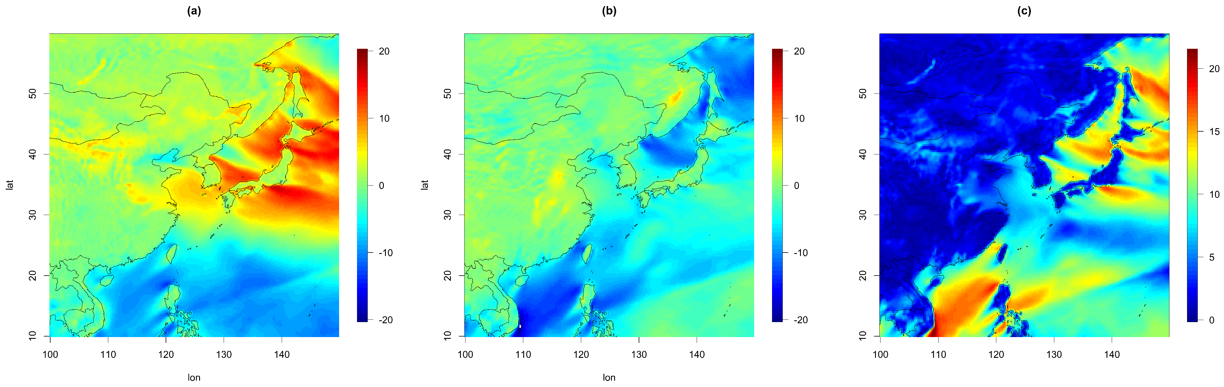
Since our focus was on wind vectors near East Asia, we used 200 longitudinal points (between and ) and 200 latitudinal points (between and ). Therefore, the full data comprise 14.6 million points () for each wind component. An example is given in Figure 1, where we present the two wind components as well as the wind speed on 1 January 2021. Here, we observe different spatial behaviors of those variables over land and ocean; for example, the wind speed is higher over the ocean than over the land.
We also examined the temporal characteristics of the daily wind components in the data. For each site, the empirical skewness and kurtosis values of the U component over time are reported in Figure 2. Here, we clearly observe some features of skewness and heavier tails (more prevalent than lighter tails) compared to the Gaussian distribution (i.e., the skewness and kurtosis are 0 and 3, respectively) in many spatial locations, and we expected a better characterization of the temporal behavior of the wind component if we considered higher moments, such as the third and fourth moments. In this case, the non-Gaussian assumption might be useful for modeling, and thus, we decided to consider a transformed Gaussian process as in [23].
Overall, the wind vectors analyzed here cover a spatial domain over land and ocean, and they also evolve daily. Therefore, multivariate models that can describe both spatial and temporal behaviors of the two wind components need to be considered. As multivariate spatio-temporal modeling is becoming the norm in the geostatistics community, we considered a space–time cross-covariance function in our modeling framework. Moreover, we employed the trans-Gaussian approach in order to relax the non-Gaussian features of the dataset, in particular, in time.
3. Method
3.1. Model
For a general setting, we consider a stochastic process as a collection of random variables at each spatial–temporal location , . Under the Gaussian assumption, the statistical behavior of is well described by its first two moments, the mean vector and the cross-covariance matrix , where is a covariance between and for . Due to this property, it is essential to take into account the valid (positive definite) space–time cross-covariance structure between variables in addition to the autocovariance structure for each of the variables [24].
On the other hand, real data, such as wind speed over time [7], often exhibit an asymmetric and light- or heavy-tailed distribution, and therefore, the first two moments are not enough to characterize the temporal behavior of the wind over time. A simple remedy is to apply a component-wise transformation to an underlying multivariate Gaussian process :
where and : , . Note that are typically obtained from the same parametric family of monotonic transformations, but their parameters are set to be different to allow for different shapes of marginal densities. The Tukey g-and-h transformation [25] and the sinh and arcsinh transformation [26] provide simple but flexible ways to construct non-Gaussian models. In this study, we adopt the Tukey g-and-h transformation, denoted as henceforth, which has the following form, with two parameters, g and h:
Here, the parameter g governs the skewness, and controls the tail behavior. Along with a location parameter and a scale parameter , provides a general marginal distribution. This transformation can be easily applied to a Gaussian process and results in flexible marginal distributions, allowing for an adjusted skewness and heavy tails. Yan and Genton [27] proposed non-Gaussian autoregressive process of order p using the Tukey g-and-h transformation, called TGH-AR(p), for time series data, and [7] successfully implemented it to model the temporal dependence structure of wind speed data. Yan et al. [23] discussed a general framework for modeling non-Gaussian multivariate stochastic processes via these transformations.
Genton and Kleiber [28] and Porcu et al. [22] provided detailed information on valid models for cross-covariance functions and space–time covariance functions. The Matérn covariance function [29] and its variations, such as the multivariate version of the Matérn covariance function [30], are popular in geostatistical modeling. In this study, we work with the parametric class of the space–time cross-covariance function proposed by [31]. The multivariate Gneiting–Matérn space–time model is
where and are space and time lags, respectively; and are the temporal range and smoothness, respectively; is the spatio-temporal interaction; is the standard deviation parameter; is the spatial range; is the spatial smoothness; and is the colocated correlation coefficient. Here, is an expression of the Matérn correlation function, where , and denotes the modified Bessel function of the second kind of the order .
In real data, the assumption of isotropy for the covariance function is often limited. Several geophysical data applications showed a strong dependence of the covariance structure on latitude [7,32,33]. A straightforward extension of (1) for nonstationarity is possible by letting the parameters vary over space or time. Note that there is always a trade-off between computational cost and model flexibility of nonstationary covariance functions; an overly complicated model may lead to infeasible computation. Thus, we should carefully balance the flexibility of the model with parsimony when determining the structure of the model. In this study, we let the covariance be different between land and ocean and vary depending on the latitudes in Section 4. This provides enough flexibility to capture the nonstationarity in the real wind data without overly complicating the model structure.
3.2. Inference Scheme
Multivariate space–time covariances often involve complicated nonstationary and high-dimensional structures. In the last two decades, various estimation techniques based on likelihood approximation have been proposed to balance statistical efficiency and computational complexity [22]. For example, new classes of scalable models, such as covariance tapering [34], fixed rank kriging [35], predictive processes [36], Gaussian Markov random fields [37], and recently, a general framework for Vecchia approximations [38], were developed and applied to various large spatial and spatio-temporal data. Although the approaches mentioned above and some other variations were benchmarked for large spatial data in [39], it is not easy to judge which approach is best in general [22].
For parameter estimation in this study, we focused on the composite likelihood approach [40] because it is relatively simple to apply compared to other approximation approaches. Varin et al. [41] provided a detailed overview of composite likelihood methods, and Bourotte et al. [31] provided an extension to multivariate space–time. The key idea is that, instead of modeling , where is a single realization from the whole field with N locations and T time points, we considered sub-densities over partitions . Here, only the subset of that belongs to was used to compute the sub-density over the partition . Then, we approximated the log-likelihood as follows:
Depending on the design of partitions and weights , the computational burden to evaluate the log-likelihood function and estimate the parameters can be significantly reduced.
We define as the bivariate spatio-temporal daily wind vector at location and time , and define . Since we apply the Tukey g-and-h transformation to the Gaussian process, our model can be written as:
where , with is a vector of the location parameters, ⨂ is the Kronecker product, and is a vector of ones of length T (length of time). Furthermore, , , and are defined similarly. In particular, and are the vectors of the parameters for the Tukey g-and-h transformation at each site; that is, we consider the element-wise transformation. Here, is the Gaussian process with zero mean vector and the covariance matrix based on the covariance function with corresponding parameters in (1). Therefore, we define , where and are the parameters of the Tukey g-and-h transformation. The total set of parameters is now .
The TGH-AR(p) model for a univariate time series proposed by [27] at each spatial location is defined as follows:
where is a Gaussian process with zero mean and constant variance , and are the autoregressive model coefficients under the weakly stationary assumption. Here, the multivariate model TGH-VAR(p) can be naturally extended. We refer to [23,27] for the model description and parameter estimation in detail.
Since is high-dimensional, we used a two-step inference scheme and assumed that the parameters obtained from the previous step are fixed and known, as follows:
- Step 1. We fit the TGH-AR(p) at each spatial location and each variable. Then, we obtained the residuals by filtering out the fitted values based on their estimated parameters of TGH-AR(p), i.e., . Here, we could select either the univariate TGH-AR(p) or the bivariate Tukey g-and-h vector autoregressive model of order p as in [23]. In any case, we could perform estimation independently at each site, i.e., the computation could be easily parallelized.
- Step 2. We fit the space–time cross-covariance model to the residuals and estimated the remaining parameters. Here, if the computation costs matter, we could sub-sample in each partition and use them for parameter estimation. In this study, we split the whole dataset into partitions (16 spatial pieces × 5 temporal pieces), and then sub-sampled approximately 15% and 15% of observations from each spatial and temporal piece, respectively. As a result, the number of data points was 78,400, which was still large enough for the parameter estimation. We tried different partition numbers (from to ) and subsampling proportions (from to ) and did not find notable changes in inference performance.
4. Results
4.1. Parameter Estimation
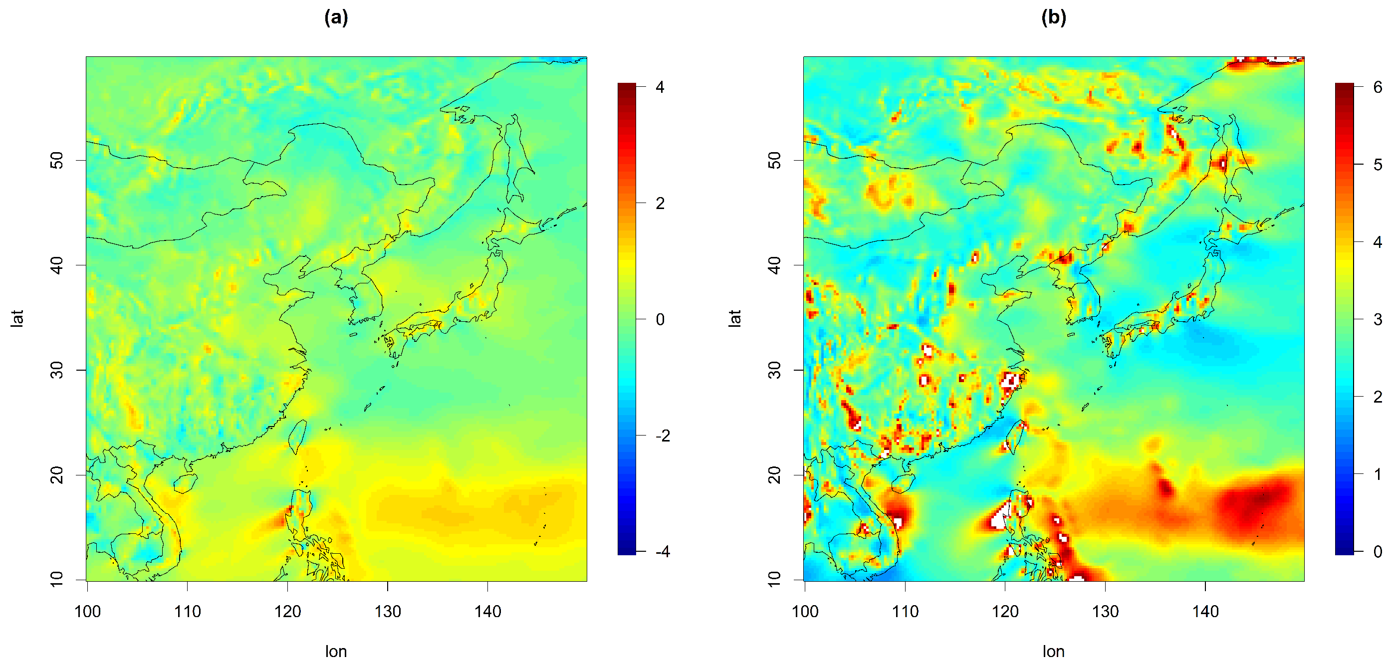
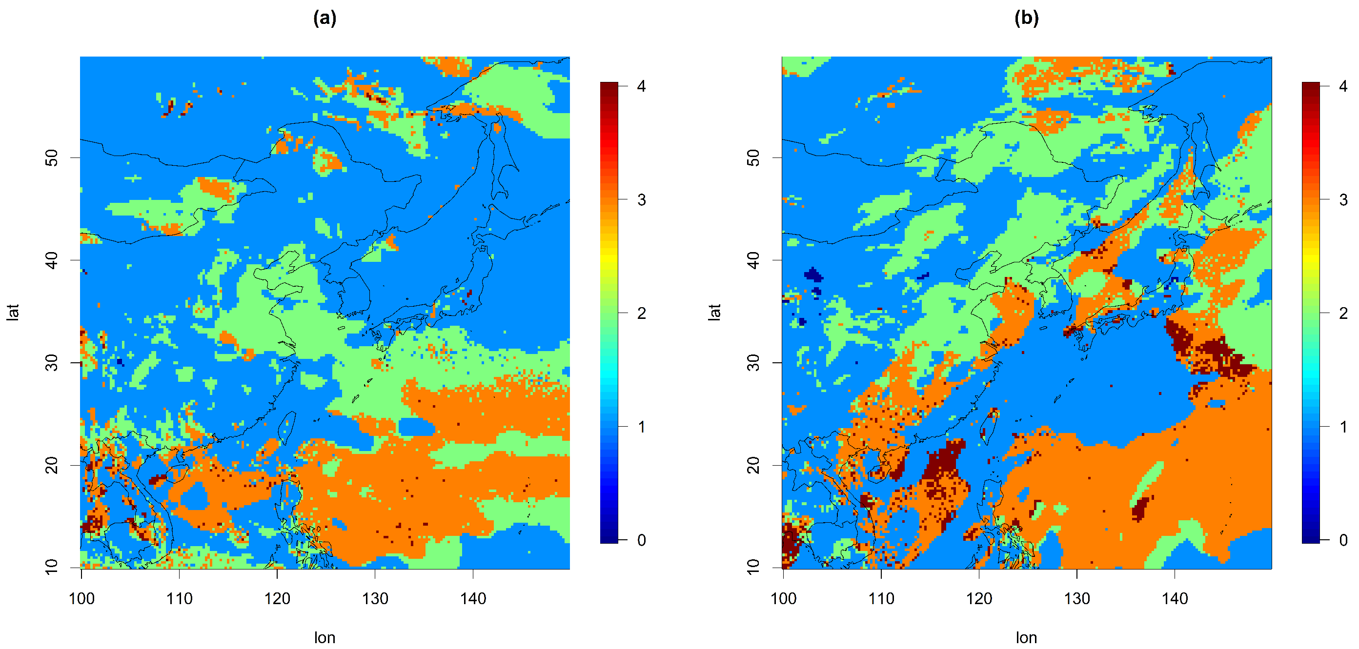
First, for both the U and V components, we fitted the univariate TGH-AR(p) at each spatial location. Setting a high order p can make the scale of the resulting residuals too small, and thus, we restricted the value (up to 4). TGH-AR(p) fitting effectively transformed the original time series to a Gaussian time series (or at least close to Gaussian). Additionally, it reduced some amount of temporal dependency. Figure 3 represents the selected order for the TGH-AR(p) fit at each site for the U and V components. was selected, except for 6 and 66 locations (out of 40,000 sites) for the U and V components, respectively. Moreover, in most locations near Korea, or were selected in the model fit. The estimated parameters of the Tukey g-and-h transformation for U are given in Figure 4. Here, nonzero values of and were obtained over most locations, indicating that the autoregressive model with the Gaussian assumption is not suitable for the U component. The remaining dependence structures were captured by the space–time cross-covariance function in Step 2. To find the residuals for both variables, we filtered out the fitted values from TGH-AR(p) at each site. Here, the variations over space were reduced as well compared to the original datasets, so we suspect that complicated and nonstationary cross-covariance models might not be required.
After obtaining the residuals and , we computed their average variances at different latitudes and time steps, as shown in Figure 5. The black circles represent the quadratic regression fit. The variances over the land and the ocean for both residuals look different, and depending on the latitude, their behaviors are also quite different. We slightly extended the cross-covariance model to further capture these nonstationary aspects in variances. To examine how the varying degree of nonstationarity specified in our model affects the prediction performance, we fitted three bivariate spatio-temporal cross-covariance models to the residuals as follows:
- Model 1: A parsimonious version of the space–time Gneiting-Matérn of (1); i.e., we assumed the same spatial range r for both variables.
- Model 2: This model was the same as Model 1, but the variances and had different values over the land and the ocean.
- Model 3: This model was the same as Model 1, but the variances and had varying values depending on the latitude over the land and the ocean. Here, we fixed the variances to their estimated values from the second-order polynomial regression in Figure 5.
Figure 5.
Variance across latitude for all residuals ( and over land and ocean).

Table 1 provides the maximum log-likelihood, Akaike information criterion (AIC), and Bayesian information criterion (BIC) values for each model. Model 2 shows a better model fitting in terms of all three considered criteria. The parameter estimates for each model are reported in Table 2.
The estimates of the colocated correlation coefficients for all models were relatively small but positive, indicating that the multivariate model should be considered. For the temporal parameters, an interesting point was observed. Model 1 has the smallest estimate for the temporal range but the largest smoothness and spatio-temporal interaction estimates for a and b (both values are close to their limits). The temporal parameters appear to be associated with the spatio-temporal interaction b. When has a small (large) value, a and b tended to have large (small) values. For the spatial parameters, the spatial range values r were estimated as 130–500 km, and the nuggets, and , for both components were estimated as very small values. Models 2 and 3 had similar estimate values of smoothness for both components of around 0.4–0.5, resulting in non-smooth spatial processes. However, the smoothness of the U component in Model 1 was estimated as a larger value than that of the V component. We suspect that Model 1 estimated the spatial range parameter by a smaller value than its competitors, while it estimated the smoothness parameter for V by a large value compared to other models. Model 1 preferentially captured the variation of V residuals, resulting in a relatively larger value than Models 2 and 3. As a result, this delivered a valid model fit for V but a bad fit for the U residuals, implying poor performance in prediction. Note that Models 2 and 3, which were based on different (or varying) effects of variances over the land and the ocean, performed estimations without leaning on a specific component. Thus, we can expect a comparable model fit for both residuals. For Model 2, the estimated standard deviations over land and ocean were notably different, implying that the use of different parameters over the land and the ocean leads to a better model fit.
4.2. Prediction
For multivariate spatio-temporal data, the tool of co-kriging is available to interpolate and predict a variable given its spatio-temporal relationship to other variables. Under the squared-error loss criterion, the simple co-kriging predictor is the best linear unbiased predictor [24]. We used co-kriging to predict wind components at unobserved space–time locations. Note that our task is to interpolate values at missing time points and spatial locations instead of forecasting the future, and the predictions considered are conditional on the future data (relative to the time point predicted).
From the training set, once we obtained estimates of , we could perform prediction with the 2 steps we considered in parameter estimation, but backward. At first, we used a bivariate Gaussian space–time process that requires mean surfaces for each component of and a proper space–time cross-covariance function. Here, represents a residual process obtained from Step 1. From the multivariate normal distribution of , we considered the following co-kriging estimate:
where is a prediction target for the first component at an unobserved space–time point, , is the covariance matrix for the residual vector of for both components provided by the estimated space–time cross-covariance function, and is a covariance vector between and the residual vector for both components. In the next step, given one variable at each spatial location, we considered prediction using the TGH-AR(p) model (we performed interpolation using AR(p) structure with all the data including the future and Tukey g-and-h transformation in order). To make our experiment simple, we added fitted values from AR(p) and then considered the Tukey g-and-h transformation. For details on prediction using the TGH-AR(p) model, we refer to [27].
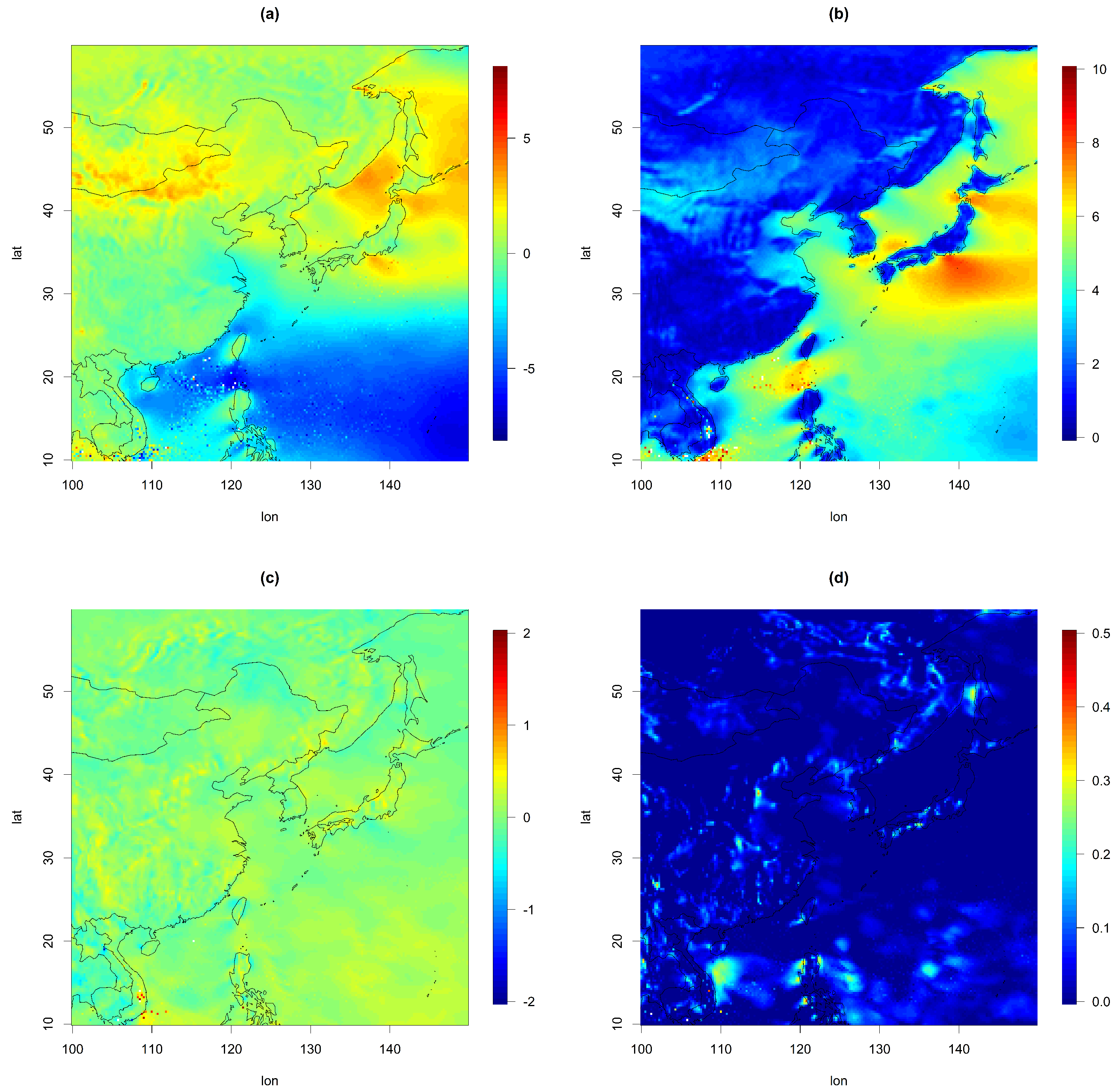
To avoid computational issues due to large amounts of data, we relied on sub-sampling. We selected 1000 locations from the map in Figure 6 in the subsequent four days from 1 July to 4 July 2021. For each day, we considered a parallelogram-shaped region (with a white dotted outline) near South Korea as in Figure 6 and randomly selected 100 and 150 locations inside and outside of the region, respectively. Except for the selected locations and time points, we treated the remaining data points as our training data for prediction. Then, we predicted the two wind components at those selected locations. We repeated this procedure by changing the prediction targets 30 times to see the variations in prediction scores. Figure 7 is one example of the predicted wind components based on Model 3 on 4 July 2021. Note that this experiment assumes a situation where the prediction model is constructed based on a much larger region and a longer time period than the test data, which leads to a harder test because the fitted parameters are not specifically optimized for the test sets.
Table 3 and Table 4 show summary statistics of prediction scores (including separate measures over the land and the ocean) for each model based on the 30 repetitions, where we sampled different locations for the test dataset for each iteration. For prediction scores, we considered the mean absolute error (MAE) and root-mean-squared error (RMSE). The prediction performances over the ocean were better than those over the land for all models. For wind velocity, the processes over the ocean are generally smoother than those over the land, and thus, we expected that the prediction was easier and resulted in more accurate predictions over the ocean than those over the land. Model 1 showed the best performance for the V component, although it had the worst performance for the U component. Model 2 showed the best model fit in terms of log-likelihood, AIC, and BIC values, although it resulted in the worst prediction in the case of the V component. Model 3 outperformed the other models for the U component and showed comparable performance to Model 1 for the V component. Here, Models 2 and 3 had a disagreement between the model fitting performance for the training data and the prediction performance for the test data. We suspect that the main reason for this was the difference in the sizes of areas covered by the training and test sets. The training dataset covered East Asia, as shown in Figure 1, while the test dataset covered the middle and southern part of the Korean peninsula, as shown in Figure 6. The fitted model’s global optimum in the training area may not be the best for the test area.
To further examine the prediction performances in detail, we plotted the absolute prediction errors for the U and V components on 3 July 2021 from 1 of the 30 repetitions in Figure 8 and Figure 9. We have chosen this particular date and the iteration because the test area covers mountainous areas in the center of South Korea and the southwestern coastal area, both of which are important for wind power generation in the nation. For Model 1, we observed somewhat high prediction errors in the U component near the boundary over the southwest regions of Korea. We suspect that the highly estimated spatial smoothness parameter for the U component led to a poor prediction performance here. The V component delivered a good prediction performance, as expected from Table 2. Since Model 1 does not have any terms to represent the strong zonal trend (i.e., the trend along the latitude), the range was set to be shorter than the other models to capture the trend, and as a result, the other parameters were optimized based on this range value, resulting in much higher smoothness than the other models. Model 2 had larger prediction errors for both wind components than Model 3 because of the abrupt change of variances near the boundary between the land and ocean areas in the prediction. Since Model 2 should solely rely on the land–ocean difference to capture all the nonstationarity in the spatial pattern, the difference between the land and the ocean is perhaps too exaggerated. Model 3 did not suffer from this issue because we adapted varying variances depending on latitudes and changed those over the land and ocean, resulting in a more flexible model than Model 2.
In practice, we often work with residuals to fit covariance models that require a flexible covariance function. There are several ways to obtain residuals, such as the method of empirical orthogonal function (EOF) [42] and spherical harmonics [43]. Our site-wise TGH-AR(p) fitting can be an alternative way to obtain residuals from space–time data. The two-step approach allows us to use a simple, valid covariance function and further save computational costs.
We also computed the predicted wind speed from the U and V components based on three models. Table 5 shows summary statistics of prediction errors of the wind speed based on each model. Overall, Model 3 outperforms other competitors in prediction errors. Model 1 tends to have the worst prediction errors for both MAE and RMSE, while Model 2 has the largest variation on RMSE with the largest maximum value due to the aforementioned land–ocean boundary issue.
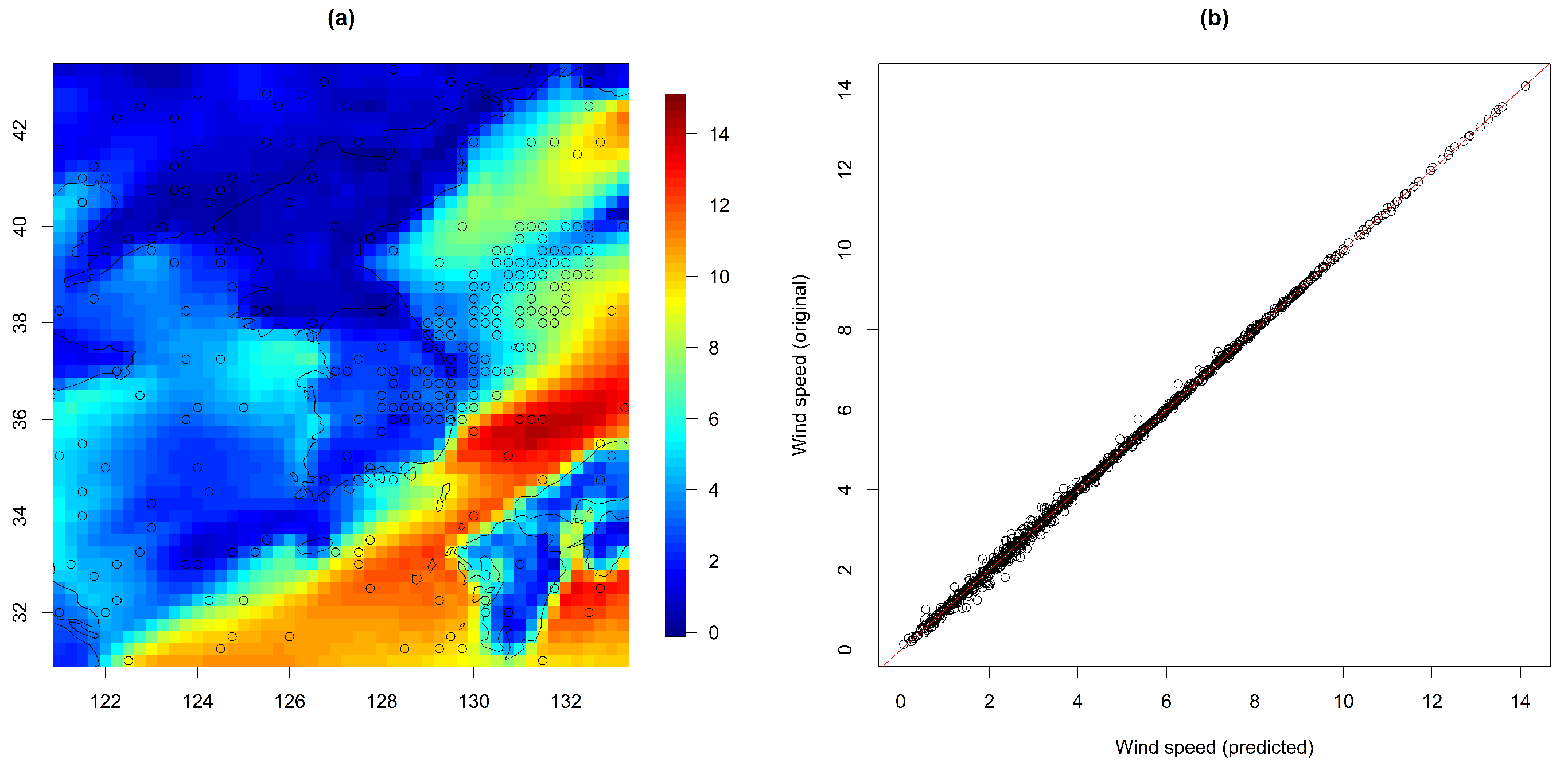
Figure 10a presents the predicted wind speed map for 4 July 2021, calculated from two wind components from Model 3. Additionally, we made a scatter plot of the predicted and original wind speed (from Model 3), showing that most observations lie close to a straight line. The co-kriging approach based on our model produced a fairly accurate prediction.
To show the utility of our approach, we assessed how better prediction in wind speed leads to better prediction in the wind power density (WPD) (in W m−2), which is often used as a metric to evaluate the availability of wind energy for power generation [44,45]. The WPD for conversion from a wind turbine can be computed as
where is the air density and is the wind speed [44,45]. In this study, we assumed kgm−3, which is the typically used air density value, as in [6].
Using the predicted wind speed values based on three models, we obtained predicted WPD values and compared them with the observed WPD values to examine the prediction performance. Summary statistics of the prediction scores for WPD values from each model based on the 30 repetitions are presented in Table 6. The difference in prediction performance is amplified compared to the results shown in Table 5 because the predicted wind speed is cubed in (2). This example shows that accurate wind speed prediction is important for predicting wind power density, a highly relevant metric for wind power generation.
5. Conclusions
In this study, we explored a non-Gaussian modeling framework for wind vectors in East Asia. The model was motivated by the Tukey g-and-h transformation to describe non-Gaussian features of wind vectors over time. The two-step inference scheme with the composite likelihood approach allows for parameter estimation with flexible dependence structures and large datasets. For the first step, the Tukey g-and-h autoregressive model described the temporal dependences of wind vectors at each site. Additionally, the independence assumption helped reduce the computational burden and modeled large-scale variations over space. The remaining variations over space and time were modeled by the bivariate Gaussian process with space–time cross-covariance. The cross-covariance function can be extended to the nonstationary version by using varying parameters for different spaces in general. In our data example, Model 3 with spatially varying variances over different latitudes outperformed competitors in prediction and hence the computation of wind power density.
Our approach has the following limitations. Firstly, Model 2 showed the best model fit, but its prediction performance was the worst for the V component among the models we considered. We suspect that the land–ocean transition error problem occurred, i.e., the sudden change between the land and the ocean produced worse prediction results, in particular, for the V component. One possible remedy is to allow a smooth transition between the land and the ocean states when we fit the model and perform predictions. In the climate application, Castruccio and Guinness [46] used the modified land–ocean indicator coupled with the Tukey taper function and demonstrated that the smooth transition approach is effective in modeling. Secondly, the models we considered are simple and limited regarding nonstationarity due to setting the same spatial range values for the land and the ocean. We believe wind vectors with large domains show strong nonstationarity in practice, and we expect that considering spatially varying parameters, such as variance, spatial range, and smoothness, in the covariance function will result in improved performance in both model fitting and prediction. The natural extension is to consider nonstationary covariance models with spatially varying parameters over some factors, such as land–ocean boundaries and different latitudes, for wind vectors and perform more intensive wind energy applications near Korea. Lastly, when we computed the wind power potential in Korea, we only focused on the daily average of wind vectors. Since the wind can blow differently in both speed and direction over time within a day, the daily average may misrepresent the wind pattern. Moreover, we need to predict future wind behavior to find optimal locations for wind turbines. In this case, one might further explore the wind vectors from the Earth System Models (ESMs) as they can provide projections of the future climate.
Author Contributions
Conceptualization, J.J. and W.C.; methodology, J.J.; software, J.J. and W.C.; data curation, J.J. and W.C.; writing—original draft preparation, J.J.; writing—review and editing, J.J. and W.C.; visualization, J.J.; supervision, W.C. All authors have read and agreed to the published version of the manuscript.
Funding
This work was supported by the research fund of Hanyang University (HY-202000000002693) and by a National Research Foundation of Korea (NRF) grant funded by the Korea government (MSIT) (No. 2021R1F1A1049185).
Data Availability Statement
The wind vector dataset can be found in the European Centre for Medium-Range Weather Forecasts (ECMWF) Renalysis v5 (https://cds.climate.copernicus.eu/cdsapp#!/dataset/reanalysis-era5-pressure-levels?tab=overview, accessed on 1 January 2023).
Conflicts of Interest
The authors declare no conflict of interest.
References
- Moomaw, W.; Yamba, F.; Kamimoto, M.; Maurice, L.; Nyboer, J.; Urama, K.; Weir, T.; Bruckner, T.; Jäger-Waldau, A.; Krey, V.; et al. Introduction. In IPCC Special Report on Renewable Energy Sources and Climate Change Mitigation; Edenhofer, O., Pichs-Madruga, R., Sokona, Y., Seyboth, K., Matschoss, P., Kadner, S., Zwickel, T., Eickemeier, P., Hansen, G., Schlömer, S., et al., Eds.; Cambridge University Press: Cambridge, UK; New York, NY, USA, 2011. [Google Scholar]
- Obama, B. The irreversible momentum of clean energy. Science 2017, 355, 126–129. [Google Scholar] [CrossRef] [PubMed]
- Barthelmie, R.; Pryor, S.C. Potential contribution of wind energy to climate change mitigation. Nat. Clim. Chang. 2014, 4, 684–688. [Google Scholar] [CrossRef]
- Koebrich, S.; Bowen, T.; Sharpe, A. 2018 Renewable Energy Data Book (No. NREL/BK-6A20-75284); National Renewable Energy Lab. (NREL): Golden, CO, USA, 2020. [Google Scholar]
- Hersbach, H.; Bell, B.; Berrisford, P.; Biavati, G.; Horányi, A.; Muñoz Sabater, J.; Nicolas, J.; Peubey, C.; Radu, R.; Rozum, I.; et al. ERA5 Hourly Data on Pressure Levels from 1979 to Present; Copernicus Climate Change Service (c3s) Climate Data Store (cds): Reading, UK, 2018; Volume 10. [Google Scholar]
- Jeong, J.; Castruccio, S.; Crippa, P.; Genton, M.G. Reducing Storage of Global Wind Ensembles with Stochastic Generators. Ann. Appl. Stat. 2018, 12, 490–509. [Google Scholar] [CrossRef]
- Jeong, J.; Yan, Y.; Castruccio, S.; Genton, M.G. A stochastic generator of global monthly wind energy with Tukey g-and-h autoregressive processes. Stat. Sin. 2019, 29, 1105–1126. [Google Scholar] [CrossRef]
- Tagle, F.; Castruccio, S.; Crippa, P.; Genton, M.G. A non-Gaussian spatio-temporal model for daily wind speeds based on a multi-variate skew-t distribution. J. Time Ser. Anal. 2019, 40, 312–326. [Google Scholar] [CrossRef]
- Chen, W.; Castruccio, S.; Genton, M.G.; Crippa, P. Current and future estimates of wind energy potential over Saudi Arabia. J. Geophys. Res. Atmos. 2018, 123, 6443–6459. [Google Scholar] [CrossRef]
- Tagle, F.; Genton, M.G.; Yip, A.; Mostamandi, S.; Stenchikov, G.; Castruccio, S. A high-resolution bilevel skew-t stochastic generator for assessing Saudi Arabia’s wind energy resources. Environmetrics 2020, 31, e2628. [Google Scholar]
- Giani, P.; Tagle, F.; Genton, M.G.; Castruccio, S.; Crippa, P. Closing the gap between wind energy targets and implementation for emerging countries. Appl. Energy 2020, 269, 115085. [Google Scholar] [CrossRef]
- Zhang, J.; Crippa, P.; Genton, M.G.; Castruccio, S. Sensitivity Analysis of Wind Energy Resources with Bayesian non-Gaussian and nonstationary Functional ANOVA. arXiv 2021, arXiv:2112.13136. [Google Scholar]
- Gualtieri, G. A comprehensive review on wind resource extrapolation models applied in wind energy. Renew. Sustain. Energy Rev. 2019, 102, 215–233. [Google Scholar] [CrossRef]
- Kim, S.; Lee, H.; Kim, H.; Jang, D.H.; Kim, H.J.; Hur, J.; Cho, Y.S.; Hur, K. Improvement in policy and proactive interconnection procedure for renewable energy expansion in South Korea. Renew. Sustain. Energy Rev. 2018, 98, 150–162. [Google Scholar] [CrossRef]
- Cripps, E.; Nott, D.; Dunsmuir, W.T.; Wikle, C. Space–Time Modelling of Sydney Harbour Winds. Aust. New Zealand J. Stat. 2005, 47, 3–17. [Google Scholar] [CrossRef]
- Ailliot, P.; Monbet, V.; Prevosto, M. An autoregressive model with time-varying coefficients for wind fields. Environmetrics 2006, 17, 107–117. [Google Scholar] [CrossRef]
- Ezzat, A.A.; Jun, M.; Ding, Y. Spatio-temporal short-term wind forecast: A calibrated regime-switching method. Ann. Appl. Stat. 2019, 13, 1484–1510. [Google Scholar] [CrossRef]
- Huang, H.; Castruccio, S.; Genton, M.G. Forecasting high-frequency spatio-temporal wind power with dimensionally reduced echo state networks. J. R. Stat. Soc. Ser. C Appl. Stat. 2022, 71, 449–466. [Google Scholar] [CrossRef]
- Ding, Y. Data Science for Wind Energy; CRC Press: Boca Raton, FL, USA, 2019. [Google Scholar]
- Chen, W.; Genton, M.G.; Sun, Y. Space-time covariance structures and models. Annu. Rev. Stat. Its Appl. 2021, 8, 191–215. [Google Scholar] [CrossRef]
- Fan, M.; Paul, D.; Lee, T.C.; Matsuo, T. Modeling tangential vector fields on a sphere. J. Am. Stat. Assoc. 2018, 113, 1625–1636. [Google Scholar] [CrossRef]
- Porcu, E.; Furrer, R.; Nychka, D. 30 Years of space–time covariance functions. Wiley Interdiscip. Rev. Comput. Stat. 2021, 13, e1512. [Google Scholar] [CrossRef]
- Yan, Y.; Jeong, J.; Genton, M.G. Multivariate transformed Gaussian processes. Jpn. J. Stat. Data Sci. 2020, 3, 129–152. [Google Scholar] [CrossRef]
- Wackernagel, H. Multivariate Geostatistics; Springer Science & Business Media: Berlin/Heidelberg, Germany, 2003. [Google Scholar]
- Tukey, J.W. Modern Techniques in Data Analysis. In Proceedings of the NSF-Sponsored Regional Research Conference, Southern Massachusetts University, North Dartmouth, MA, USA, 1977; Volume 7. [Google Scholar]
- Jones, M.C.; Pewsey, A. Sinh-arcsinh distributions. Biometrika 2009, 96, 761–780. [Google Scholar] [CrossRef]
- Yan, Y.; Genton, M.G. Non-Gaussian autoregressive processes with Tukey g-and-h transformations. Environmetrics 2019, 30, e2503. [Google Scholar] [CrossRef]
- Genton, M.G.; Kleiber, W. Cross-covariance functions for multivariate geostatistics. Stat. Sci. 2015, 30, 147–163. [Google Scholar] [CrossRef]
- Matérn, B. Spatial Variation; Springer Science & Business Media: Berlin/Heidelberg, Germany, 2013; Volume 36. [Google Scholar]
- Gneiting, T.; Kleiber, W.; Schlather, M. Matérn cross-covariance functions for multivariate random fields. J. Am. Stat. Assoc. 2010, 105, 1167–1177. [Google Scholar] [CrossRef]
- Bourotte, M.; Allard, D.; Porcu, E. A flexible class of non-separable cross-covariance functions for multivariate space–time data. Spat. Stat. 2016, 18, 125–146. [Google Scholar] [CrossRef]
- Kleiber, W.; Nychka, D. Nonstationary modeling for multivariate spatial processes. J. Multivar. Anal. 2012, 112, 76–91. [Google Scholar] [CrossRef]
- Jun, M. Matérn-based nonstationary cross-covariance models for global processes. J. Multivar. Anal. 2014, 128, 134–146. [Google Scholar] [CrossRef]
- Furrer, R.; Genton, M.G.; Nychka, D. Covariance Tapering for Interpolation of Large Spatial Datasets. J. Comput. Graph. Stat. 2006, 15, 502–523. [Google Scholar] [CrossRef]
- Cressie, N.; Johannesson, G. Fixed Rank Kriging for Very Large Spatial Data Sets. J. R. Stat. Soc. Ser. B (Stat. Methodol.) 2008, 70, 209–226. [Google Scholar] [CrossRef]
- Banerjee, S.; Gelfand, A.E.; Finley, A.O.; Sang, H. Gaussian Predictive Process Models for Large Spatial Data Sets. J. R. Stat. Soc. Ser. B (Stat. Methodol.) 2008, 70, 825–848. [Google Scholar] [CrossRef]
- Lindgren, F.; Rue, H.; Lindström, J. An Explicit Link Between Gaussian Fields and Gaussian Markov Random Fields: The Stochastic Partial Differential Equation Approach. J. R. Stat. Soc. Ser. B (Stat. Methodol.) 2011, 73, 423–498. [Google Scholar] [CrossRef]
- Katzfuss, M.; Guinness, J. A general framework for Vecchia approximations of Gaussian processes. Stat. Sci. 2021, 36, 124–141. [Google Scholar] [CrossRef]
- Heaton, M.J.; Datta, A.; Finley, A.O.; Furrer, R.; Guinness, J.; Guhaniyogi, R.; Gerber, F.; Gramacy, R.B.; Hammerling, D.; Katzfuss, M.; et al. A case study competition among methods for analyzing large spatial data. J. Agric. Biol. Environ. Stat. 2019, 24, 398–425. [Google Scholar] [CrossRef] [PubMed]
- Lindsay, B.G. Composite likelihood methods. Contemp. Math. 1988, 80, 221–239. [Google Scholar]
- Varin, C.; Reid, N.; Firth, D. An overview of composite likelihood methods. Stat. Sin. 2011, 21, 5–42. [Google Scholar]
- Hannachi, A.; Jolliffe, I.T.; Stephenson, D.B. Empirical orthogonal functions and related techniques in atmospheric science: A review. Int. J. Climatol. J. R. Meteorol. Soc. 2007, 27, 1119–1152. [Google Scholar] [CrossRef]
- Jeong, J.; Jun, M. A class of Matérn-like covariance functions for smooth processes on a sphere. Spat. Stat. 2015, 11, 1–18. [Google Scholar] [CrossRef]
- Peterson, E.W.; Hennessey, J.P., Jr. On the Use of Power Laws for Estimates of Wind Power Potential. J. Appl. Meteorol. 1978, 17, 390–394. [Google Scholar] [CrossRef]
- Newman, J.; Klein, P. Extrapolation of Wind Speed Data for Wind Energy Applications. In Proceedings of the Fourth Conference on Weather, Climate, and the New Energy Economy. Annual Meeting of the American Meteorological Society, Austin, TX, USA, 5–7 January 2013; Volume 7. [Google Scholar]
- Castruccio, S.; Guinness, J. An evolutionary spectrum approach to incorporate large-scale geographical descriptors on global processes. J. R. Stat. Soc. Ser. C (Appl. Stat.) 2017, 66, 329–344. [Google Scholar] [CrossRef]
Figure 1.
Wind components, (a) U and (b) V. (c) Wind speed on 1 January 2021.

Figure 2.
(a) Skewness and (b) kurtosis of U over time.

Figure 3.
Plot of the selected order for TGH-AR(p) for (a) U and (b) V (ms−1).

Figure 4.
Plot of the estimated parameters for the Tukey g-and-h transformation, with (a) , (b) , (c) g, and (d) h for U.
Figure 4.
Plot of the estimated parameters for the Tukey g-and-h transformation, with (a) , (b) , (c) g, and (d) h for U.

Figure 6.
Selected prediction locations from 1–4 July 2021 (U values in color).

Figure 7.
Predicted (a) U and (b) V (ms−1) on 4 July 2021 from Model 3.

Figure 8.
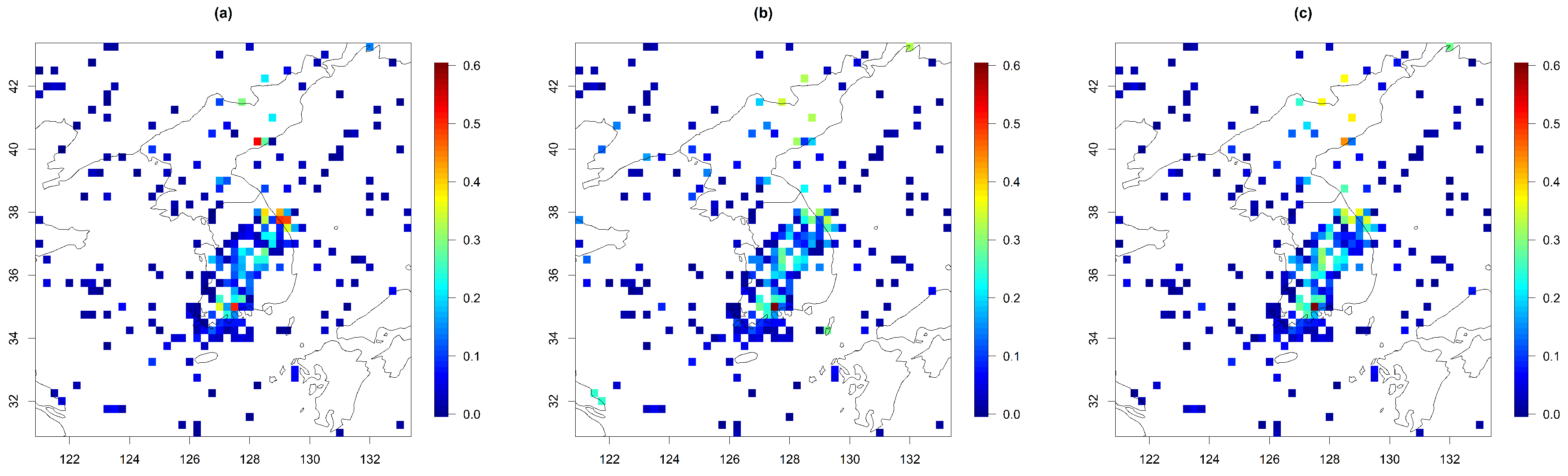
Absolute prediction errors of the U component for (a) Model 1, (b) Model 2, and (c) Model 3 on 3 July 2021 (for 1 case out of the 30 repetitions).
Figure 8.
Absolute prediction errors of the U component for (a) Model 1, (b) Model 2, and (c) Model 3 on 3 July 2021 (for 1 case out of the 30 repetitions).

Figure 9.
Absolute prediction errors of the V component for (a) Model 1, (b) Model 2, and (c) Model 3 on 3 July 2021 (for 1 case out of the 30 repetitions).
Figure 9.
Absolute prediction errors of the V component for (a) Model 1, (b) Model 2, and (c) Model 3 on 3 July 2021 (for 1 case out of the 30 repetitions).

Figure 10.
(a) Predicted wind speed on 4 July 2021, and (b) scatter plot of the predicted and original wind speeds from Model 3.
Figure 10.
(a) Predicted wind speed on 4 July 2021, and (b) scatter plot of the predicted and original wind speeds from Model 3.


Table 1.
Log-likelihood, AIC, and BIC values for each model.
| Number of Parameters | Log-Likelihood | AIC | BIC | |
|---|---|---|---|---|
| Model 1 | 11 | 519.433 | −1016.865 | −914.900 |
| Model 2 | 13 | 650.794 | −1275.589 | −1155.084 |
| Model 3 | 9 | 525.153 | −1032.306 | −948.880 |
Table 2.
Parameter estimates for each model.
| a | b | r | |||||
|---|---|---|---|---|---|---|---|
| Model 1 | 0.259 | 0.930 | 0.999 | 0.999 | 131.059 | 4.685 | 0.853 |
| Model 2 | 0.065 | 1296.877 | 0.745 | 507.661 | 0.513 | 0.524 | |
| Model 3 | 0.155 | 4392.535 | <0.001 | <0.001 | 429.204 | 0.394 | 0.393 |
| Model 1 | 1.427 | 1.427 | 0.700 | 0.700 | <0.001 | ||
| Model 2 | 0.907 | 0.668 | 0.905 | 0.692 | <0.001 | <0.001 | |
| Model 3 | <0.001 | <0.001 |
Table 3.
Summary statistics of prediction measures of U for each model based on the 30 repetitions.
| U | Model 1 | Model 2 | Model 3 | |||
|---|---|---|---|---|---|---|
| MAE (Land/Ocean) | RMSE (Land/Ocean) | MAE (Land/Ocean) | RMSE (Land/Ocean) | MAE (Land/Ocean) | RMSE (Land/Ocean) | |
| Min | 0.135 (10.174/0.103) | 0.187 (0.229/0.146) | 0.051 (0.085/0.030) | 0.089 (0.127/0.059) | 0.044 (0.066/0.026) | 0.072 (0.093/0.045) |
| 0.136 (0.189/0.109) | 0.192 (0.248/0.155) | 0.056 (0.097/0.034) | 0.104 (0.149/0.067) | 0.046 (0.078/0.028) | 0.079 (0.115,0.047) | |
| 0.139 (0.192/0.112) | 0.196 (0.253/0.158) | 0.060 (0.101/0.037) | 0.113 (0.158/0.075) | 0.047 (0.082/0.029) | 0.083 (0.122/0.051) | |
| Mean | 0.139 (0.192/0.111) | 0.196 (0.251/0.158) | 0.060 (0.104/0.037) | 0.117 (0.166/0.078) | 0.047 (0.081/0.029) | 0.084 (0.121/0.053) |
| 0.142 (0.195/0.113) | 0.200 (0.255/0.163) | 0.062 (0.109/0.039) | 0.120 (0.171/0.080) | 0.048 (0.084/0.030) | 0.086 (0.127/0.056) | |
| Max | 0.144 (0.205/0.117) | 0.207 (0.268/0.170) | 0.094 (0.158/0.059) | 0.256 (0.367/0.166) | 0.052 (0.091/0.033) | 0.095 (0.141/0.069) |
Table 4.
Summary statistics of prediction measures of V for each model based on the 30 repetitions.
| V | Model 1 | Model 2 | Model 3 | |||
|---|---|---|---|---|---|---|
| MAE (land/Ocean) | RMSE (Land/Ocean) | MAE (Land/Ocean) | RMSE (Land/Ocean) | MAE (Land/Ocean) | RMSE (Land/Ocean) | |
| Min | 0.042 (0.073/0.022) | 0.076 (0.115/0.038) | 0.057 (0.099/0.030) | 0.104 (0.148/0.056) | 0.050 (0.084/0.026) | 0.090 (0.132/0.042) |
| 0.045 (0.078/0.025) | 0.089 (0.129/0.043) | 0.061 (0.105/0.036) | 0.110 (0.165/0.069) | 0.051 (0.090/0.030) | 0.097 (0.142/0.054) | |
| 0.046 (0.083/0.026) | 0.091 (0.140/0.049) | 0.064 (0.112/0.038) | 0.120 (0.172/0.077) | 0.054 (0.096/0.031) | 0.101 (0.150/0.058) | |
| Mean | 0.046 (0.082/0.027) | 0.094 (0.140/0.054) | 0.065 (0.113/0.038) | 0.125 (0.181/0.079) | 0.054 (0.096/0.032) | 0.103 (0.152/0.062) |
| 0.047 (0.085/0.029) | 0.096 (0.144/0.062) | 0.066 (0.119/0.040) | 0.128 (0.188/0.083) | 0.056 (0.100/0.033) | 0.106 (0.161/0.067) | |
| Max | 0.056 (0.101/0.034) | 0.133 (0.175/0.108) | 0.097 (0.165/0.059) | 0.254 (0.366/0.162) | 0.064 (0.110/0.040) | 0.131 (0.180/0.107) |
Table 5.
Summary statistics of prediction measures of wind speed for each model based on the 30 repetitions.
Table 5.
Summary statistics of prediction measures of wind speed for each model based on the 30 repetitions.
| Speed | Model 1 | Model 2 | Model 3 | |||
|---|---|---|---|---|---|---|
| MAE | RMSE | MAE | RMSE | MAE | RMSE | |
| Min | 0.102 | 0.150 | 0.054 | 0.093 | 0.049 | 0.083 |
| 0.104 | 0.157 | 0.055 | 0.099 | 0.051 | 0.090 | |
| 0.106 | 0.159 | 0.059 | 0.106 | 0.053 | 0.092 | |
| Mean | 0.107 | 0.159 | 0.059 | 0.111 | 0.053 | 0.093 |
| 0.109 | 0.162 | 0.062 | 0.114 | 0.054 | 0.096 | |
| Max | 0.115 | 0.174 | 0.076 | 0.205 | 0.062 | 0.112 |
Table 6.
Summary statistics of prediction measures of WPD for each model (30 repetitions).
| WPD | Model 1 | Model 2 | Model 3 | |||
|---|---|---|---|---|---|---|
| MAE | RMSE | MAE | RMSE | MAE | RMSE | |
| Min | 3.937 | 7.064 | 1.724 | 3.339 | 1.612 | 3.206 |
| 4.179 | 7.676 | 1.834 | 3.868 | 1.757 | 3.386 | |
| 4.261 | 7.885 | 1.993 | 4.276 | 1.866 | 3.749 | |
| Mean | 4.282 | 7.909 | 1.984 | 4.416 | 1.863 | 3.755 |
| 4.405 | 8.165 | 2.086 | 4.561 | 1.949 | 3.945 | |
| Max | 4.600 | 8.827 | 2.427 | 7.317 | 2.169 | 4.787 |
Disclaimer/Publisher’s Note: The statements, opinions and data contained in all publications are solely those of the individual author(s) and contributor(s) and not of MDPI and/or the editor(s). MDPI and/or the editor(s) disclaim responsibility for any injury to people or property resulting from any ideas, methods, instructions or products referred to in the content. |
© 2023 by the authors. Licensee MDPI, Basel, Switzerland. This article is an open access article distributed under the terms and conditions of the Creative Commons Attribution (CC BY) license (https://creativecommons.org/licenses/by/4.0/).
Share and Cite
MDPI and ACS Style
Jeong, J.; Chang, W. Analysis of East Asia Wind Vectors Using Space–Time Cross-Covariance Models. Remote Sens. 2023, 15, 2860. https://doi.org/10.3390/rs15112860
AMA Style
Jeong J, Chang W. Analysis of East Asia Wind Vectors Using Space–Time Cross-Covariance Models. Remote Sensing. 2023; 15(11):2860. https://doi.org/10.3390/rs15112860
Chicago/Turabian StyleJeong, Jaehong, and Won Chang. 2023. "Analysis of East Asia Wind Vectors Using Space–Time Cross-Covariance Models" Remote Sensing 15, no. 11: 2860. https://doi.org/10.3390/rs15112860
Note that from the first issue of 2016, this journal uses article numbers instead of page numbers. See further details here.