
Improved Identification for Point-Distributed Coded Targets with Self-Adaption and High Accuracy in Photogrammetry

1
School of Geosciences and Surveying Engineering, China University of Mining and Technology (Beijing), Beijing 100083, China
2
School of Geographic and Environment Science, Tianjin Normal University, Tianjin 300387, China
3
State Key Laboratory of Precision Measuring Technology and Instruments, Tianjin University, Tianjin 300072, China
*
Author to whom correspondence should be addressed.
†
These authors contributed equally to this work.
Remote Sens. 2023, 15(11), 2859; https://doi.org/10.3390/rs15112859
Submission received: 18 April 2023
/
Revised: 18 May 2023
/
Accepted: 26 May 2023
/
Published: 31 May 2023
(This article belongs to the Section Remote Sensing Image Processing)
Abstract
:A robust and effective method for the identification of point-distributed coded targets (IPCT) in a video-simultaneous triangulation and resection system (V-STARS) was reported recently. However, its limitations were the setting of critical parameters, it being non-adaptive, making misidentifications in certain conditions, having low positioning precision, and its identification effect being slightly inferior to that of the V-STARS. Aiming to address these shortcomings of IPCT, an improved IPCT, named I-IPCT, with an adaptive binarization, a more precise ellipse-center localization, and especially an invariance of the point–line distance ratio (PLDR), was proposed. In the process of edge extraction, the adaptive threshold Gaussian function was adopted to realize the acquisition of an adaptive binarization threshold. For the process of center positioning of round targets, the gray cubic weighted centroid algorithm was adopted to realize high-precision center localization. In the template point recognition procedure, the invariant of the PLDR was used to realize the determination of template points adaptively. In the decoding procedure, the invariant of the PLDR was adopted to eliminate confusion. Experiments in indoor, outdoor, and unmanned aerial vehicle (UAV) settings were carried out; meanwhile, sufficient comparisons with IPCT and V-STARS were performed. The results show that the improvements can make the identification approximately parameter-free and more accurate. Meanwhile, it presented a high three-dimensional measurement precision in close-range photogrammetry. The improved IPCT performed equally well as the commercial software V-STARS on the whole and was slightly superior to it in the UAV test, in which it provided a fantastic open solution using these kinds of coded targets and making it convenient for researchers to freely apply the coded targets in many aspects, including UAV photogrammetry for high-precision automatic image matching and three-dimensional real-scene reconstruction.
1. Introduction
Coded targets play an important role in close-range photogrammetry, machine vision, computer vision, and industrial measurements [1,2]. Each coded target has its distinct number of coding sequences, so they always serve as tie points or control points. For this reason, coded targets can be specially applied in fast image matching, object tracking, and automatic high-precision camera orientation [3,4,5]. According to their application areas, coded targets can be used in robot navigation, augmented reality, close-range/UAV photogrammetry, and many other fields [6,7]. For example, Chan et al. adopted coded targets to realize self-localization of an uncalibrated camera [5]. The authors of [8] used coded targets as tie points between images to help realize bundle adjustment and in [9], they used coded targets as control points to perform automatic resection to obtain the camera’s external orientation elements.
The coded targets include two representative common types: the ring-distributed type and the point-distributed type. The ring-distributed type is represented by Schneider circular coded targets (SCTs) [10] and the point-distributed type is represented by Geodetic Systems Inc. (GSI) coded targets (GCTs) [11].
Before using the coded targets above, it is key to identify the coding sequence number. The identification methods for SCTs were reported publicly and used in the professional photogrammetric software Agisoft Metashape [12,13] to automatically perform image matching and three-dimensional (3D) reality reconstruction in unmanned aerial vehicle (UAV) photogrammetry. The GCTs are mainly used and embedded in an industrial digital close-range photogrammetric system, named the video-simultaneous triangulation and resection system (V-STARS) [14]. As V-STARS is closed-source software, the detailed method of GCT identification is not publicly available [15]. There were few open-access peer-reviewed articles until the authors of [16] recently shared their detailed identification method for GCTs. As the authors of [16] mentioned, the structure of a GCT is more complex, but it is more stable for identification. Thus, it is of great significance to study the identification of GCTs.
The authors of [16] detail the groundbreaking work previously carried out by our group, in which clear ideas were provided for the identification of GCTs and the software program was made public. This software showed nearly equivalent results compared to V-STARS, and can be regarded as a state-of-the-art method for the identification of point-distributed coded targets (IPCTs). It is known that different sizes of measured objects in different scenarios require different shooting distances, which also correspond to the different sizes of the coded targets. As Brown et al. [14] introduced in V-STARS, 3 mm, 6 mm, and 12 mm are the most commonly used for close-range photogrammetry. It is important to keep the parameters unchangeable to obtain the correct results under different scenarios. However, in Ref. [16], the precision of center positioning was low and it produced misidentifications under certain conditions. In addition, some critical parameters needed to be tuned manually, which proved not to be flexible or self-adaptive when facing different scenarios. To improve the performance of IPCT, we propose an improved IPCT (I-IPCT) to address these shortcomings, where a more precise ellipse center positioning method and an invariance of the point–line distance ratio (PLDR) were adopted in the identity verification of a GCT and in the decoding procedure. Through these improvements, the identification of GCTs reached a perfect level with parameter self-adaptation, which approximates parameter-free conditions and is more accurate.
2. Methods
Before introducing the improved method, I-IPCT, our previous work on developing IPCT and the existing problems are discussed.
2.1. Previous Work
IPCT includes three main parts: round target extraction and center positioning, template point recognition, and decoding point determination. In the following section, the related knowledge and identification method of IPCT is briefly discussed.
2.1.1. The Structure of a GCT
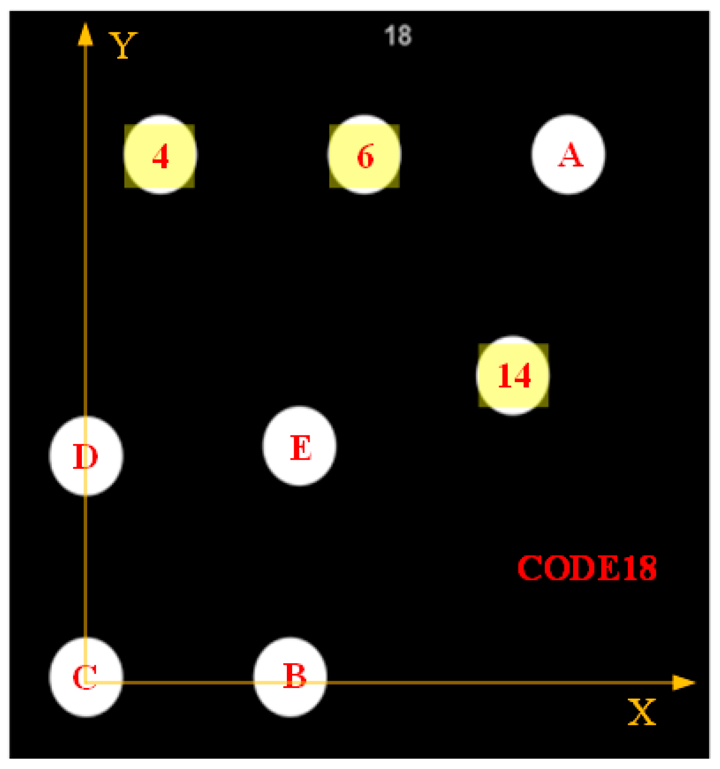
As shown in Figure 1, a GCT consists of eight round target points, including five template points and three coding/decoding points. Taking CODE18 as an example, it consists of template points A, B, C, D, and E and coding/decoding points 4, 6, and 14. Different combinations of coding points may obtain different coding sequence numbers.
2.1.2. Round Target Extraction and Center Positioning
The round targets are obtained through contour extraction, an ellipse filter with geometric constraints, and ellipse fitting. Then, the center of each target is obtained by center positioning through solving the ellipse equation.
2.1.3. Template Point Recognition
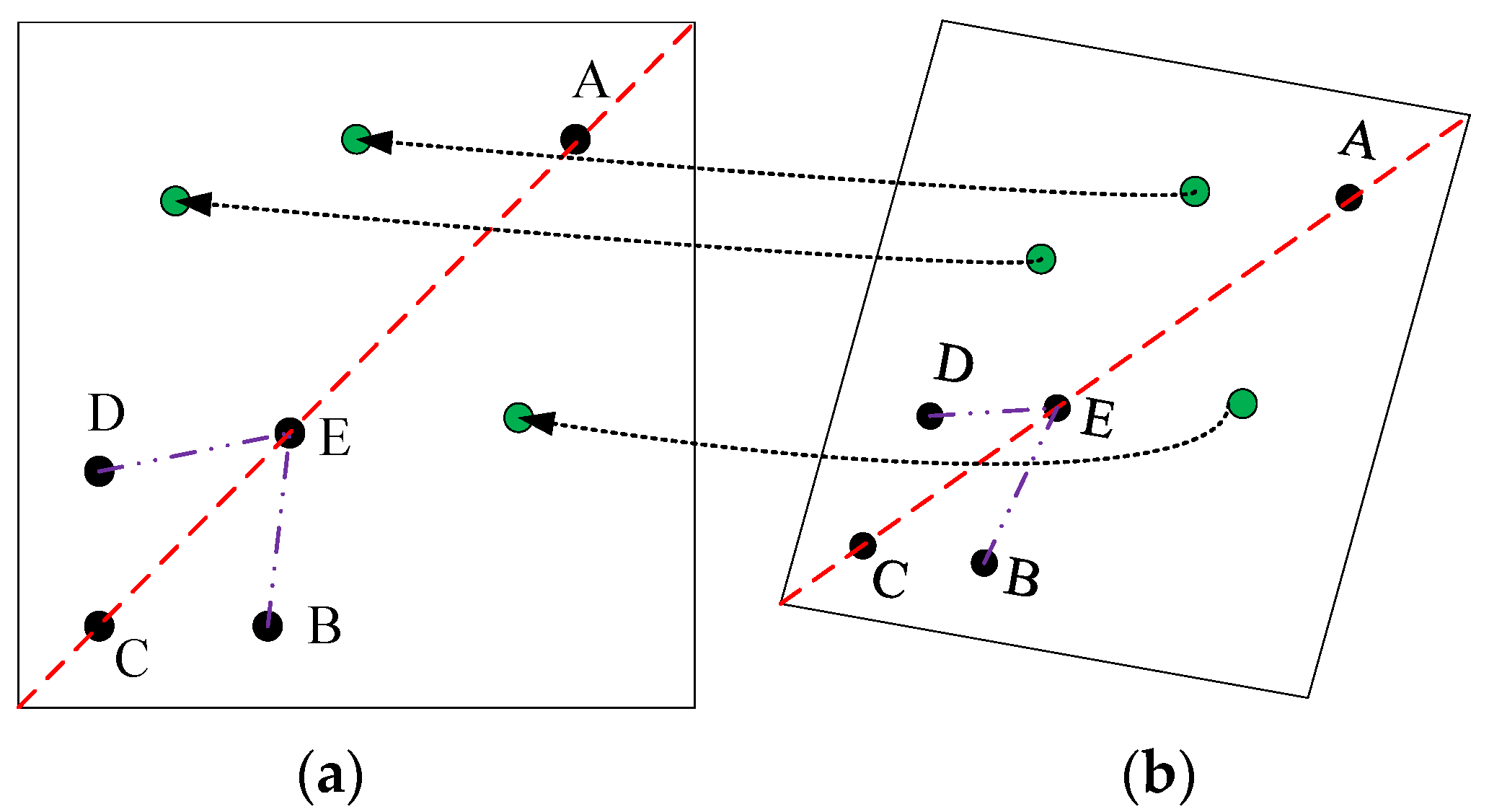
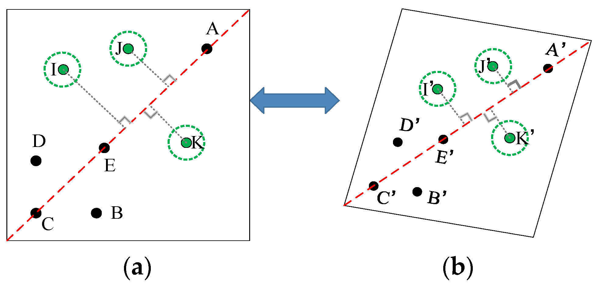
Based on Figure 2, IPCT uses the projective and permutation invariant (P2-Invariant) to achieve template point recognition. The five black dots and three green dots represent the template point and decoding point, respectively.
The value of P2-Invariant is the key to achieving template point recognition. The workflow of template point recognition is as follows:
(1) Find the three collinear points C, E, and A. (2) Find the suitable points D and B from the remaining five points. The suitable condition is the one where the calculated P2-Invariant is equal to the designed P2-Invariant.
To avoid false choices, D and B are constrained by the geometric distance restricted condition.
where is the distance from E to D or B, and is empirically calculated as 2.5.
2.1.4. Decoding Point Determination
After the five template points are determined, the affine transformation parameters between the designed plane and the imaging plane can be obtained.
Then, the three decoding points under the image coordinate system are transformed by the affine transformation parameters to obtain their corresponding calculated points under the designed coordinate system. Comparing the calculated points with the designed points in the coding library, the decoding points which satisfy the distance constraint are selected:
where is empirically set as 1.0.
After the five template points and the three decoding points are determined, a GCT can be identified.
2.1.5. Identification Process of GCTs
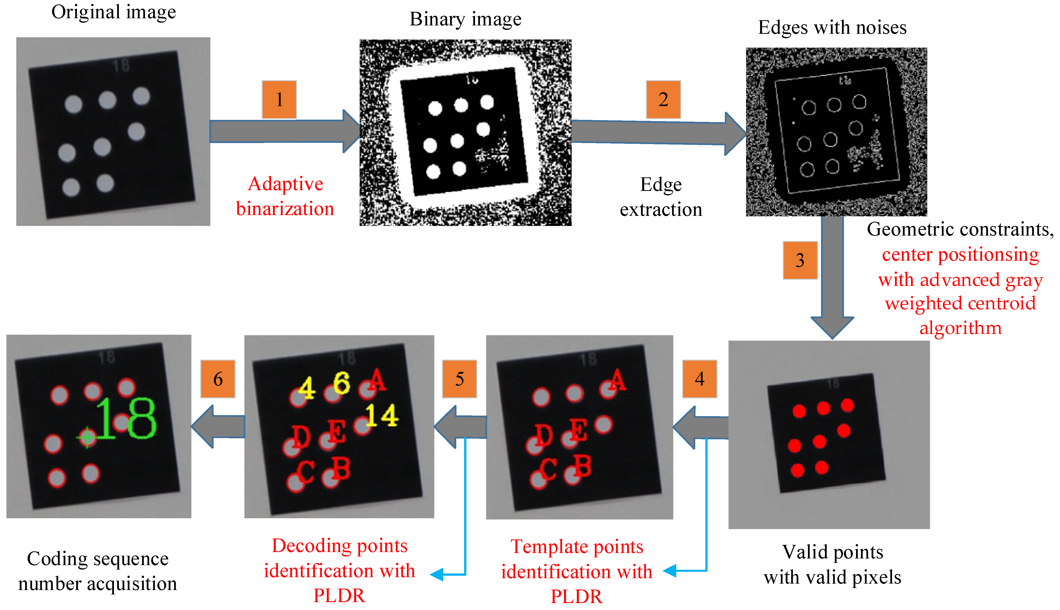
The identification process of GCTs in IPCT contains six main procedures: (1) binarization; (2) edge extraction; (3) geometric constraints, ellipse fitting, and center positioning; (4) template point identification; (5) decoding point identification; and (6) coding serial number acquisition. The details can be found in Ref. [16].
2.1.6. Existing Problems
In the procedure of the above identification process in IPCT, there exist mainly three problems.
Firstly, at the edge extraction stage, the binarization threshold is manually set with a given value according to specific lighting conditions and is not adaptive under challenging lighting conditions.
Secondly, at the center positioning stage, the centers of round targets are obtained by fitting the ellipse edge, whose localization precision is as low as 0.2–0.3 px. As V-STARS has a precision of center positioning as high as 0.02 px, which can be regarded as the standard, it is urgent to improve the center positioning precision of IPCT.
Thirdly, at the template point recognition stage and decoding point determination stage, two empirical parameters, in Equation (1) and in Equation (2), which are directly related to the Euclidean distances, are not flexible and cannot be adjusted self-adaptively. Tests have shown that when the shooting angle is larger, the method will be restricted by the constraints to some extent as the image deformation is larger. Evidently, as shown in Figure 2, when the image deformation increases, the distance difference between and increases, and should be adjusted manually. In addition, when the potential decoding points are too close or there exists some interference, misidentifications will occur. Obviously, is not anti-jamming. In brief, and should be manually tuned according to different application scenes and they cannot be easily controlled.
Due to these limitations, we developed an improved IPCT, which includes three aspects of improvement, to optimize the identification. I-IPCT includes an adaptive binarization for edge detection, a more precise center localization for round targets, and an invariance of the PLDR to replace the constraint conditions in Equations (1) and (2) for template point recognition and decoding point determination.
2.2. Adaptive Binarization for Edge Detection
The manual binarization threshold in IPCT is not convenient for complex scenarios. Here, we adopted adaptive threshold Gaussian functions to automatically calculate the threshold value for binarization.
where is the original gray value of and is a threshold calculated individually for each pixel.
where the threshold value is a weighted sum of the × neighborhood of minus and is the block size of a pixel neighborhood that is used to calculate a threshold value for the pixel: 3, 5, 7, and so on. C is a constant. are the Gaussian filter coefficients.
where , , and is the scale factor chosen so that . is the Gaussian standard deviation and is computed from K.
2.3. More Precise Ellipse-Center Localization
Ellipse fitting in IPCT is not applicable to high-precision 3D measurements. Here, we adopted an advanced gray weighted centroid algorithm to achieve a more precise localization for the ellipse center.
The unified model of gray weighted centroid algorithm is:
where is the centroid of a round target, is the gray value at inside a round target, is a parameter threshold related to the gray value, and is the weighted index for the gray value ( = 1, 2, 3…). It is equivalent to the traditional gray weighted centroid calculation formula when and , and to the gray square weighted centroid method when . Through sufficient experiments, we found the best parameters were and .
2.4. The Invariance Theory of PLDR
The theory of invariance of PLDR was originally from Refs. [17,18], which implemented line-feature matching for two images. The theory adopted point matches from scale invariant feature transform (SIFT) [19] to guide line matching. Here, we regarded the coded target identification as feature matching for two images because the designed GCT plane can be regarded as the left image and the affined GCT plane can be regarded as the right image.
2.4.1. The Invariance of the PLDR for Line Matching
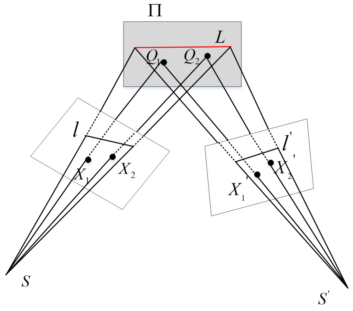
As shown in Figure 3, there exists a three-dimensional line on the object space plane. and are the corresponding two-dimensional lines on the two images. and ( = 1, 2) are the corresponding points, and ( = 1, 2) are the intersections of and on the object plane.
The invariance of the point–line distance ratio is expressed as the ratio of the distance between two points and the line. When , , and are coplanar, the points and lines on the two camera planes can be associated by a homograph. A more special affine transformation matrix can be used in the local small plane region.
where is the scale factor.
On the two camera planes, the distance ratio between two points and a line can be expressed as:
Substituting Equation (7) into Equation (8), we obtain Equation (9):
Equation (9) indicates that the distance ratio between two points, and the reference line on the left image is equal to the distance ratio between the two corresponding points and the corresponding line on the right image. This invariant serves as a basis for line matching.
The matching degree is measured by the similarity expressed in Equation (10). The larger the similarity, the higher the matching degree. The maximum of the similarity is 1.0.
The above shows the principle of PLDR invariance for line matching. It should be pointed out that the corresponding points are known and the line is to be matched.
2.4.2. The Invariance of the PLDR for Template Point Recognition
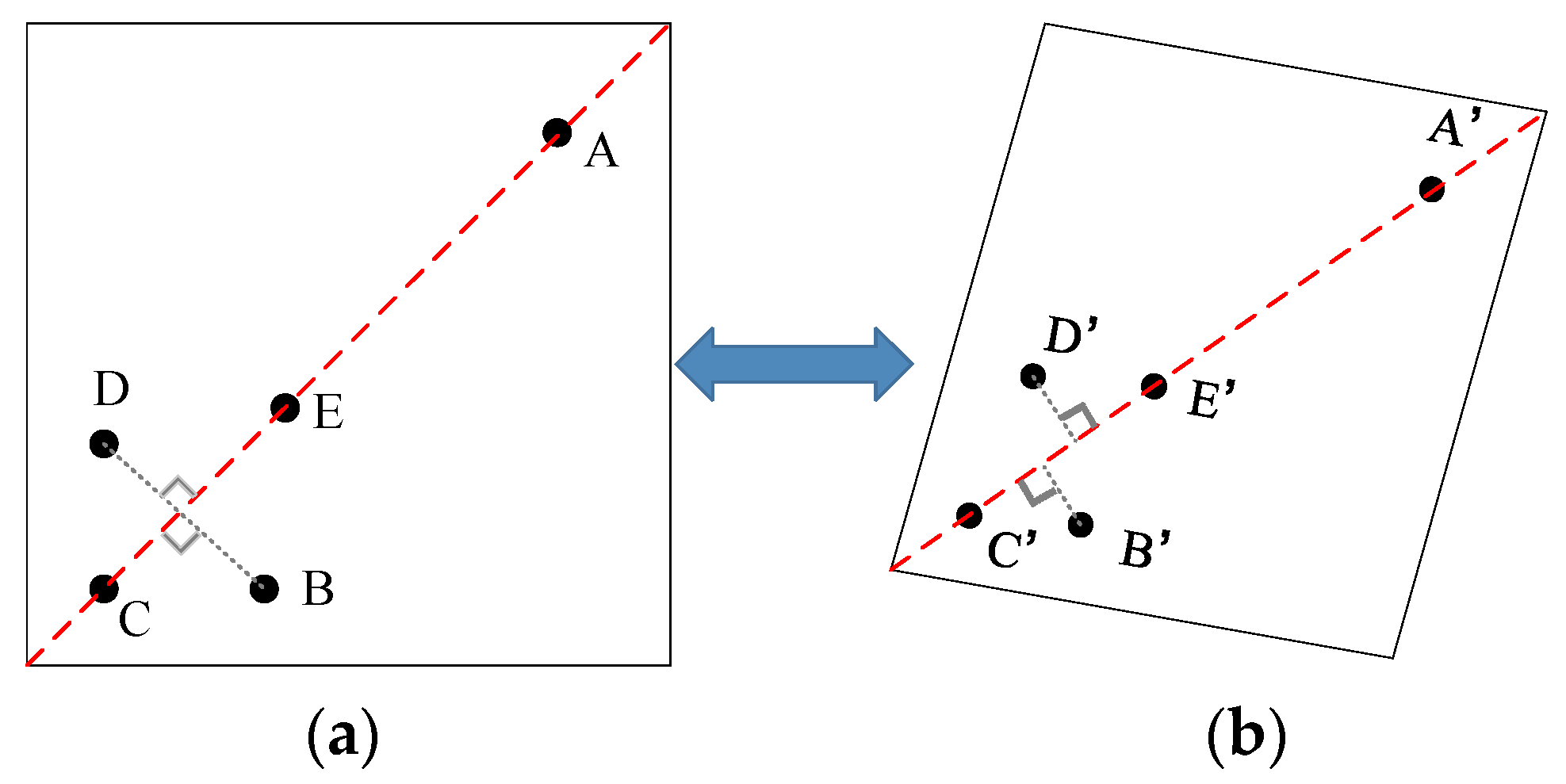
The essence of template point recognition is template point matching. That is, what we should address is how to match the affined template points (Figure 4b) with the designed template points (Figure 4a). Here, we apply the invariance of the PLDR in reverse. is the line to be matched and (,) and (,) are the corresponding points. To recognize the template points, how to match and with and , respectively, becomes a problem when the corresponding line is known.
Here, we replace Equation (1) with Equation (11) to constrain the template point matching.
As D and B are symmetrical with respect to line as designed, the ideal PLDR value associated with the template points remains constant as 1.0 under any affined transformation. However, the actual PLDR value will have a divergence of 1.0. Then, Equation (12) can be served as the criterion by which to find D and B.
2.4.3. The Invariance of the PLDR for Decoding Point Determination
Similar to template point matching, decoding point determination depends on the matching of three decoding points. That is, we should address how to match the affined decoding points (Figure 5b) with the designed decoding points (Figure 5a). Different from Equation (6), which provides a predefined distance threshold directly, we first roughly set an initial sufficient range constraint for the distance difference (refer to the green dashed circle shown in Figure 5), as shown in Equation (13); then, we adopted the invariance of the PLDR associated with the decoding points to constrain the matching precisely, as shown in Equation (14).
where represents the average diameter length of all ellipses of a GCT. is a constant scale factor. Because can be self-adapted and is built-in, the threshold is also self-adapted.
The three decoding points should satisfy the constraint in Equation (14) at the same time. To screen out the optimal three decoding points from the twenty-eight points in the coding library, the maximum of the average of the sum of similarities serves as the criterion, as shown in Equation (15):
2.5. The Identification Process of the Improved IPCT
The complete procedures of the improved IPCT are shown in Figure 6. I, J, and K correspond to decoding points 4, 6, and 14, respectively. Steps 2 and 6 are the same as the procedures in IPCT. Steps 1, 3, 4, and 5 are the important innovative parts of I-IPCT. In IPCT, the binarization is not self-adaptive; the center positioning precision is low by ellipse fitting; the template point identification is based on the P2-Invariant embedded with the geometric distance restricted condition (Equation (1)); and the decoding point identification is based on affine transformation embedded with the geometric distance restricted condition (Equation (6)). In the improved IPCT, the binarization is self-adaptive under changing lighting conditions; the positioning precision of the ellipse center is high using an advanced gray weighted centroid algorithm; the template point identification is based on the P2-Invariant embedded with the PLDR (Equation (12)), and the decoding point identification is based on affine transformation embedded with the PLDR (Equation (15)).
3. Results
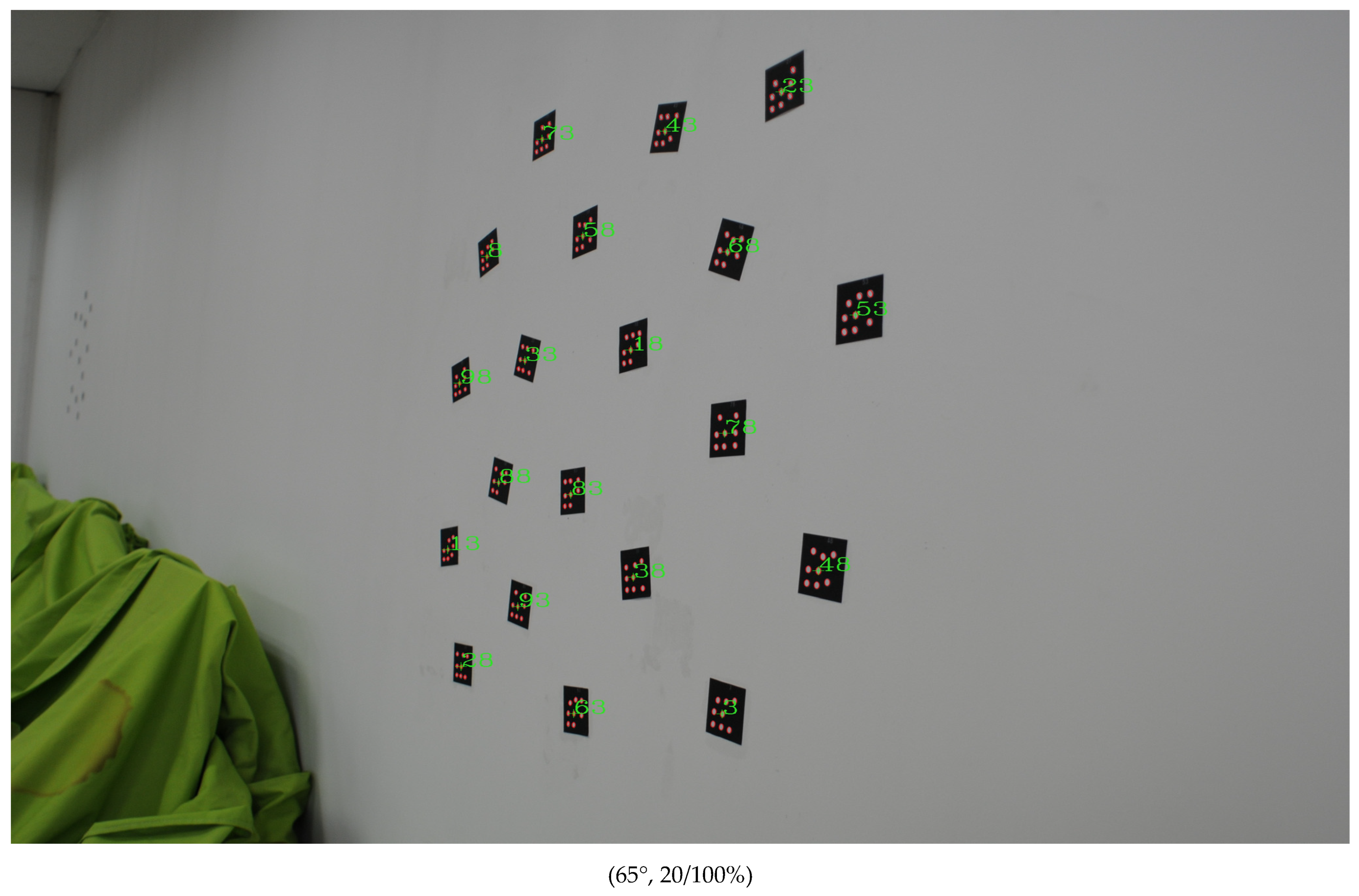
The experimental data GSI_CodedTarget_Identification (GCTI) provided by IPCT was used as the object of the test. The test data included images captured from indoor, outdoor, and UAV scenes. The identification results of V-STARS and IPCT served as comparisons, which will not be shown here again as they can be found in Ref. [16]. We provide the detailed identification results of the improved IPCT visually. The cross intersection marked by the green color is the positioning center of each GCT. The parameters below each image denote the viewing angle, correct identifications, and accurate identification rate. For outdoor and UAV scenes, different scenes were distinguished by brightness and shooting height, respectively. Empirically, I-IPCT is applicable to any experimental conditions when is set as 0.06 and is set as 0.2.
Before the final results are presented, taking a sample as an example, the intermediate results of adaptive binarization and gray cubic weighted centroid calculation are shown in Figure 7 and Figure 8.
3.1. Experiment for Indoor Scenes
3.1.1. Experiments with Different Viewing Angles of Medium-Sized GCTs
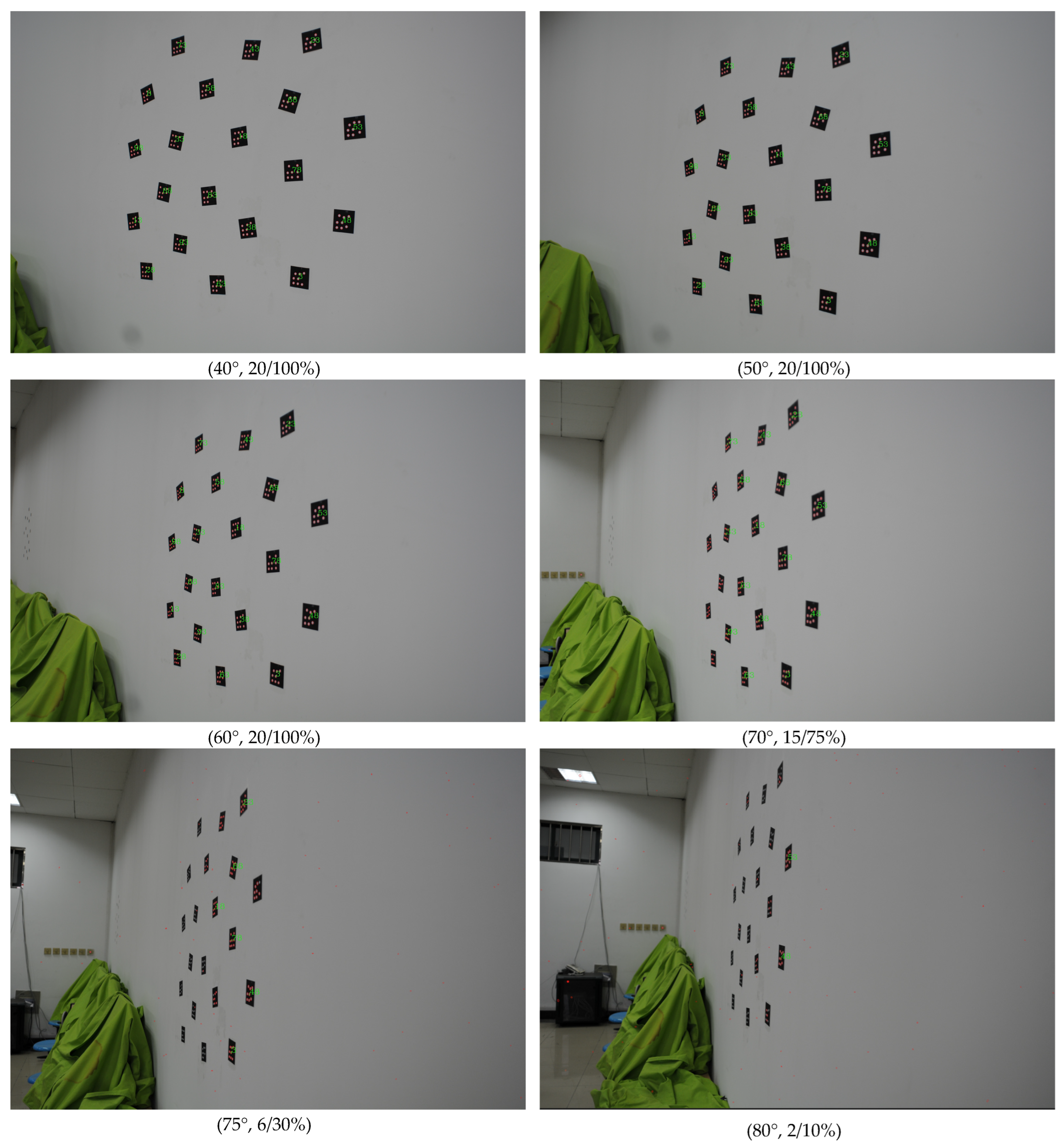
The first indoor test used twenty 6 mm diameter GCTs and the shooting distance was 2 m. The viewing angles included 0, 10, 20, 30, 40, 50, 60, 65, 70, 75, and 80°. To depict the legend better, the result at a viewing angle of 65° served as a representative result (Figure 9) and the results using the other viewing angles are shown in the Appendix A (Figure A1).
As shown in Figure 9 and Figure A1, and Ref. [16], compared with IPCT, the improved IPCT results were approximate when the viewing angle was within 60° but obviously prevailed when the viewing angle was larger than 60°. That is, the effect improved significantly when the viewing angle was 65°, 70°, 75°, and 80°. In addition, compared with V-STARS, the improved IPCT performed better overall when the viewing angle was within 70°, and it was slightly inferior to V-STARS at 75° and 80°.
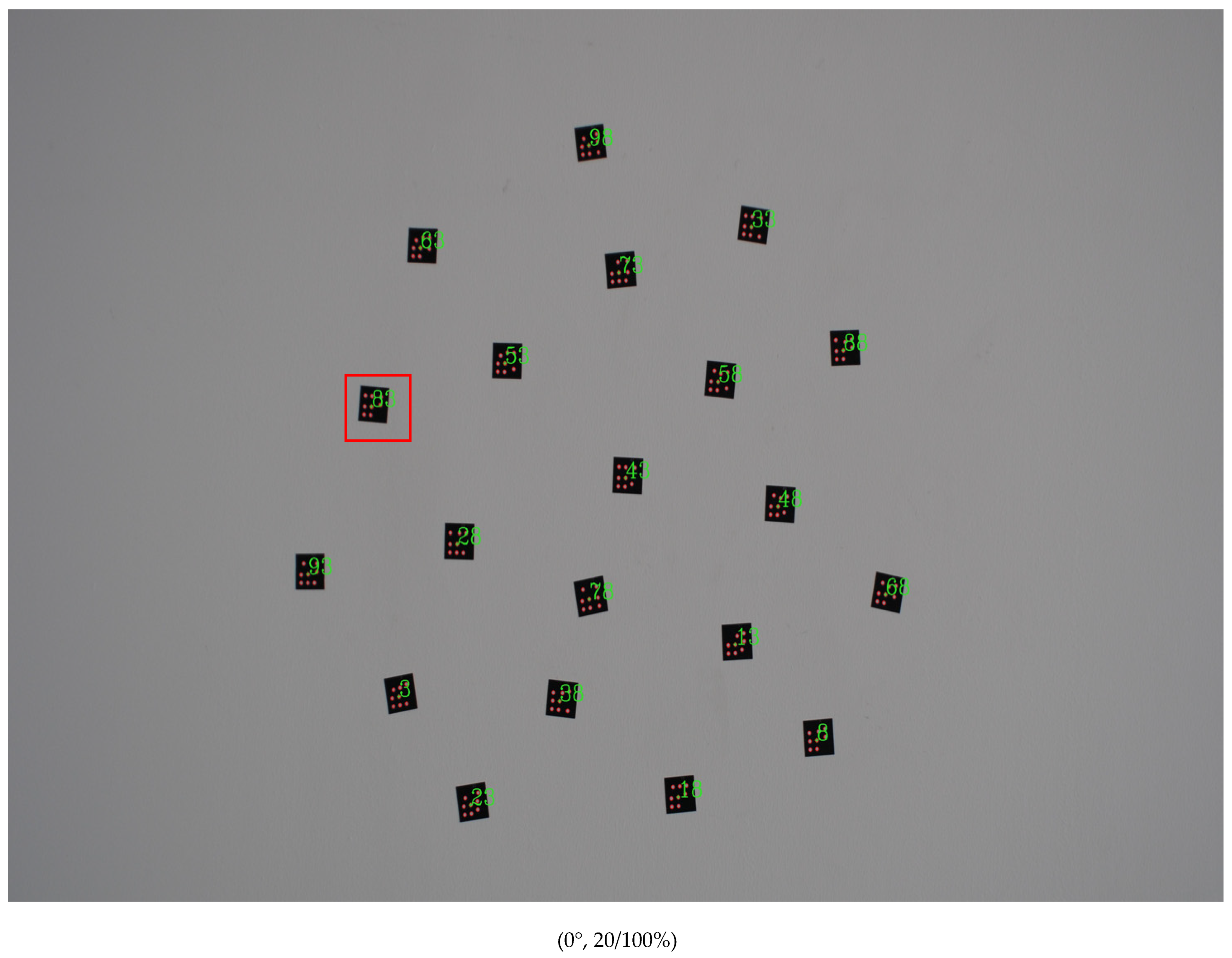
3.1.2. Experiments with Small-Sized GCTs
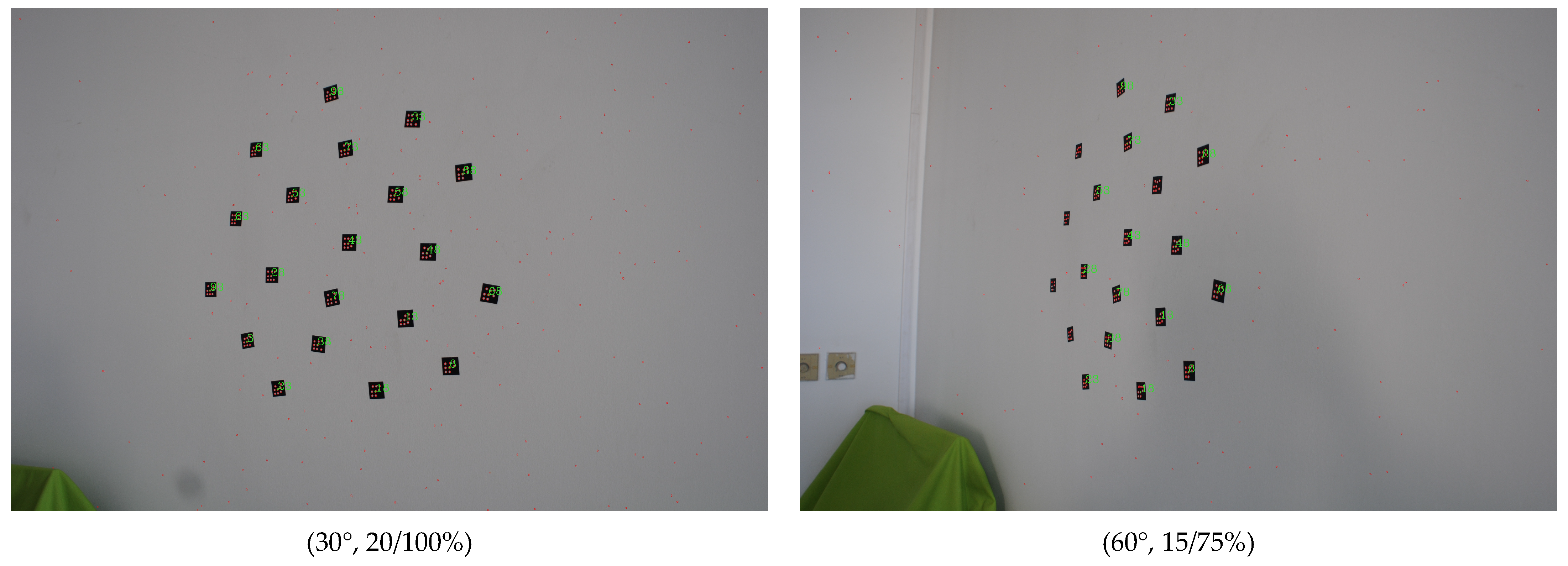
The second indoor test used twenty 3 mm diameter GCTs; the shooting distance was 1 m at viewing angles of 0, 30, and 60°. The result at viewing angle 0° served as a representative result (Figure 10) and the results using the other viewing angles are shown in the Appendix A (Figure A2).
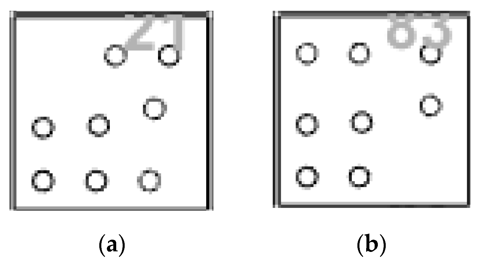
The identification results of the improved IPCT were better than those of IPCT and slightly inferior to those of V-STARS, as shown in Figure 10 and Figure A2, and Ref. [16]. Compared with IPCT, the accurate identification rate of the improved IPCT increased by 15% when the viewing angle was 60°. In particular, processed by IPCT at 0°, CODE83 (marked with a red rectangle in Figure 10) was misidentified as CODE21, but the improved IPCT correctly identified CODE83. Through observation and analysis from the outline shape of CODE21 (Figure 11a) and CODE83 (Figure 11b), the positions of some individual decoding points of CODE21 and CODE83 were very close to one another, which is prone to inducing misidentification.
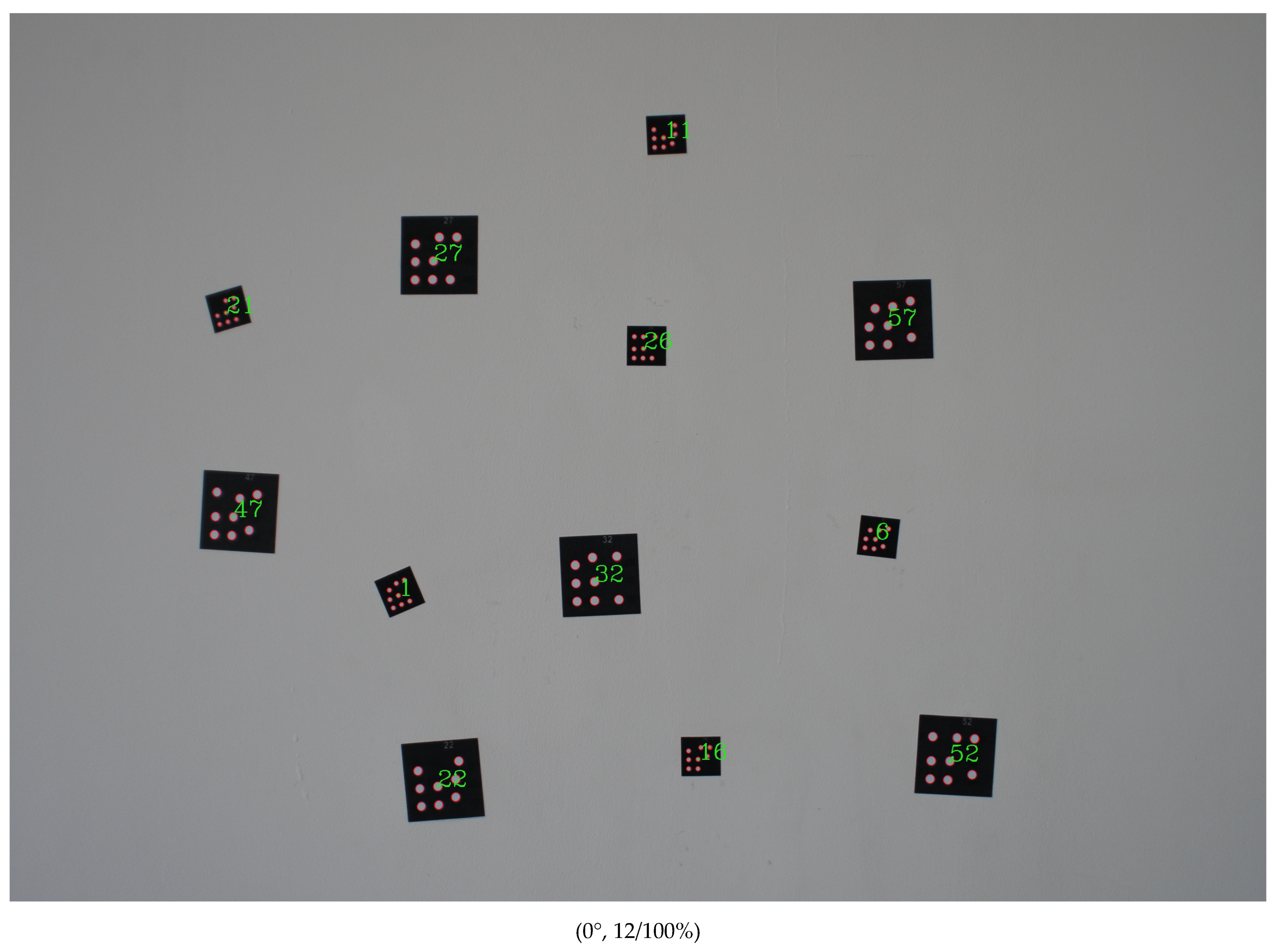
3.1.3. Experiments with Mixed GCTs
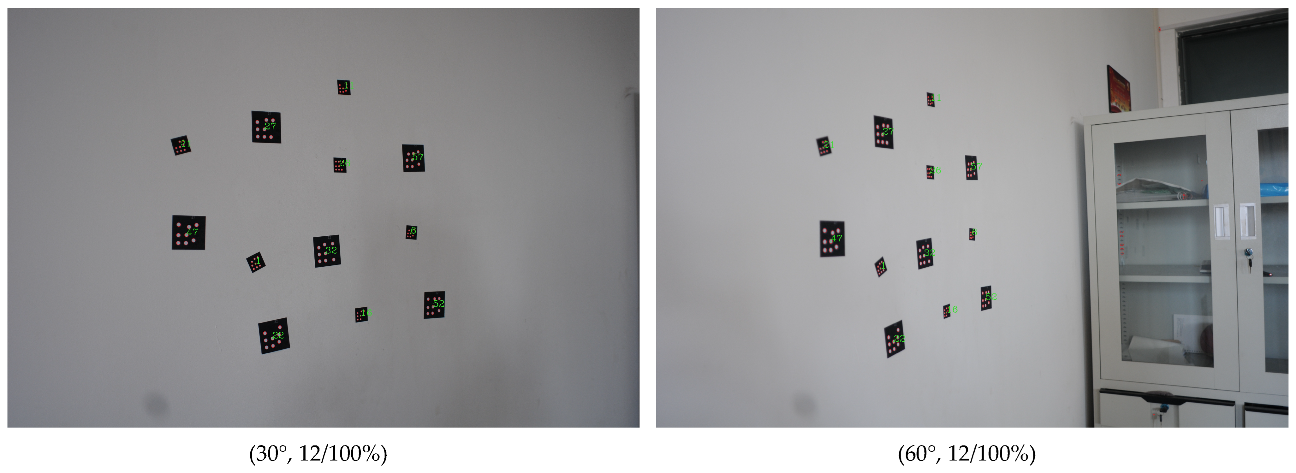
Six 6 mm diameter GCTs and six 3 mm diameter GCTs were mixed and pasted on a wall. The shooting distance was 1.5 m at viewing angles of 0, 30, and 60°. The result at a viewing angle of 0° served as a representative result (Figure 12), and the results using the other viewing angles are shown in the Appendix A (Figure A3).
Comparing the results shown in Figure 12 and Figure A3, and Ref. [16], we can see that the improved IPCT identified all of the GCTs correctly in any situation, which was similar to the performance of IPCT. As V-STARS could only correctly identify half of the GCTs at a viewing angle of 60°, the improved IPCT was superior in performance. Through careful observation of the image at a viewing angle of 60°, we found that the area where the GCTs were not identified was a little bit fuzzy. As this will affect ellipse extraction, we can infer that the method of ellipse extraction in V-STARS is different from that of the improved IPCT.
3.2. Experiment for Outdoor Scenes
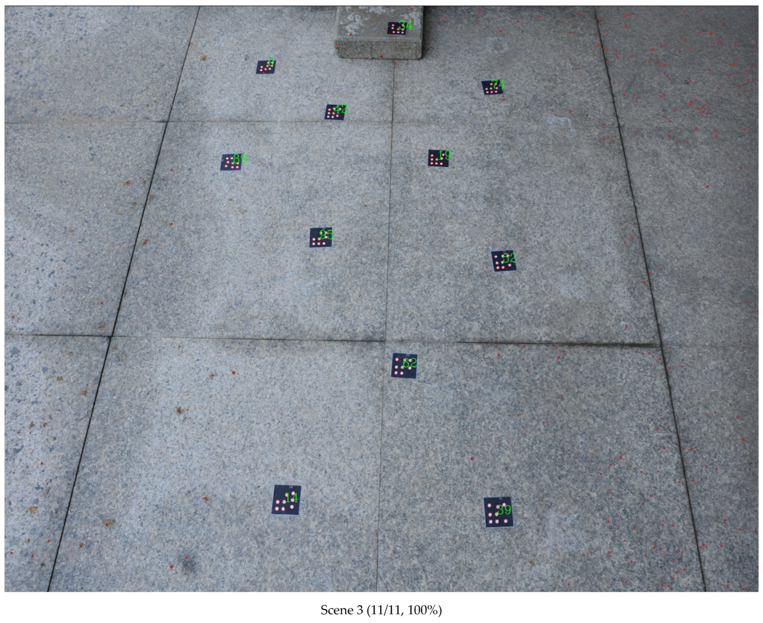
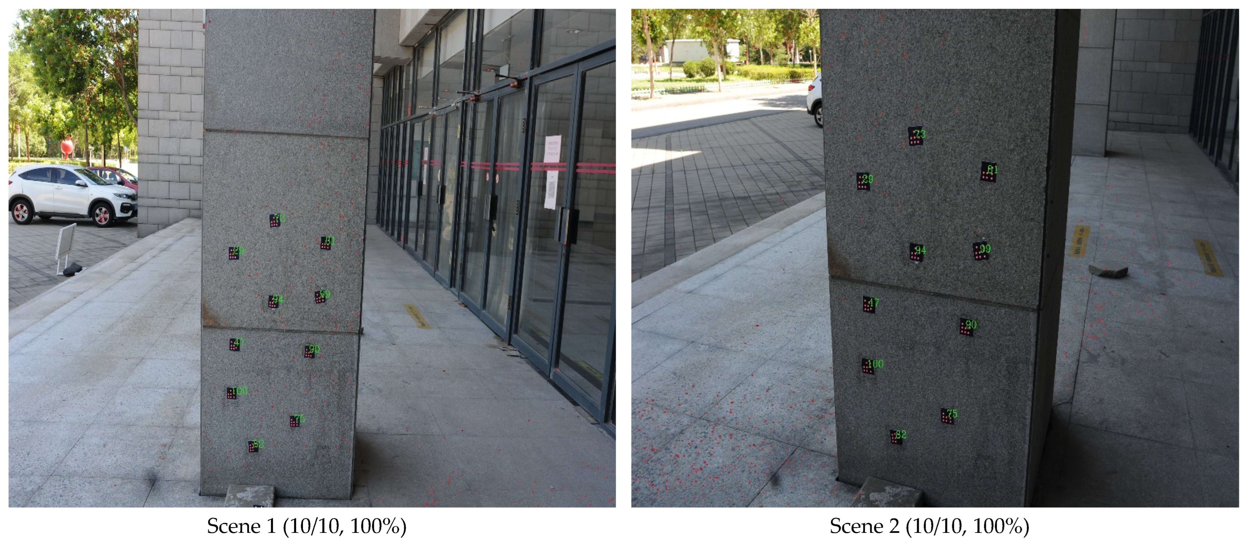
The outdoor test used eleven 6 mm diameter GCTs, and the brightness was challenging to some extent. The result of scene 3 served as a representative result (Figure 13), and the results of the other scenes are shown in the Appendix A (Figure A4).
Referring to the results in Ref. [16], the performance of the improved IPCT was similar to those of IPCT and V-STARS according to the results of scene 1 and scene 2. However, it prevailed over the other two methods as it correctly identified all the GCTs, as shown from the results of scene 3.
3.3. Experiment for UAV Scenes
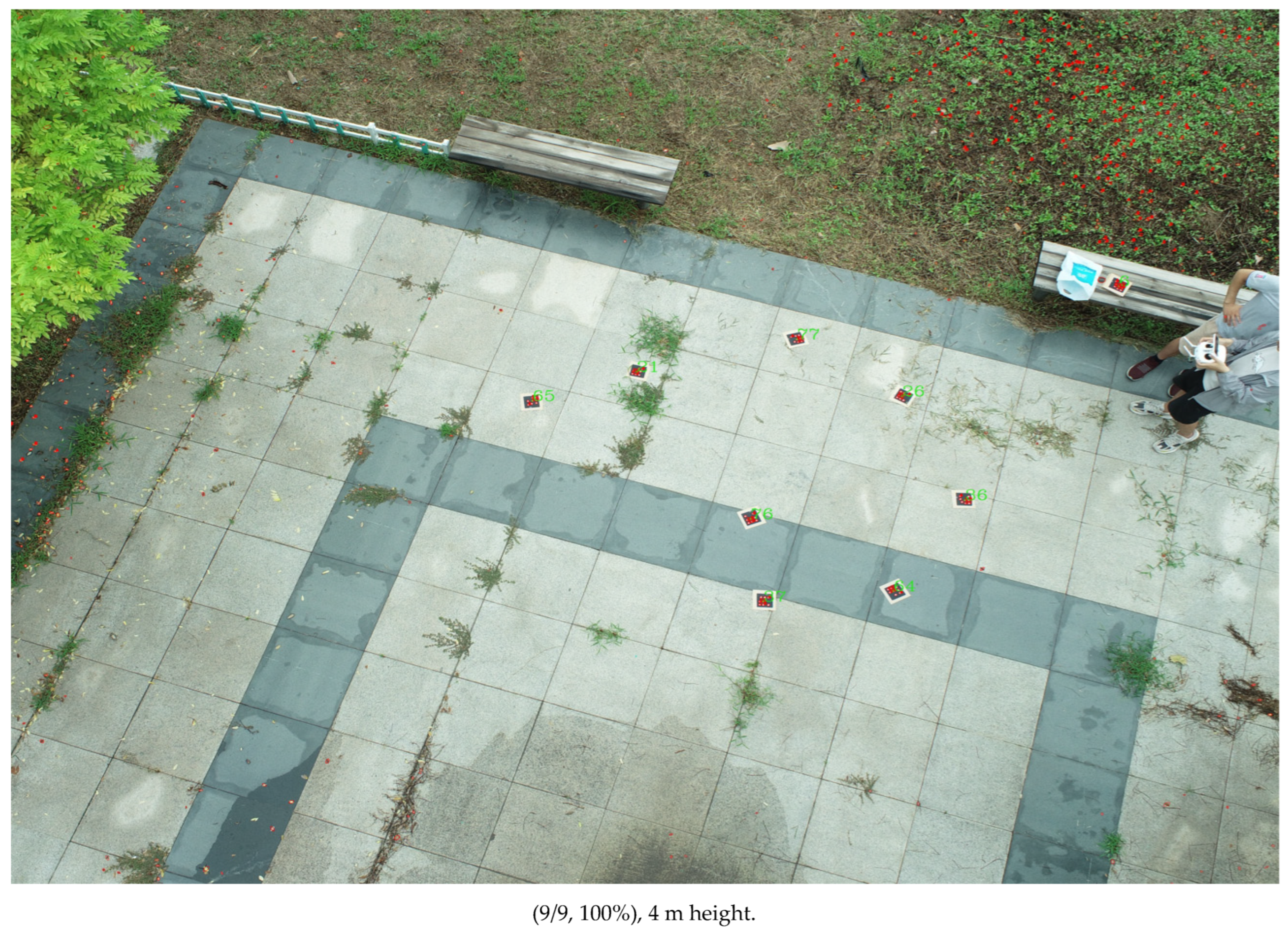
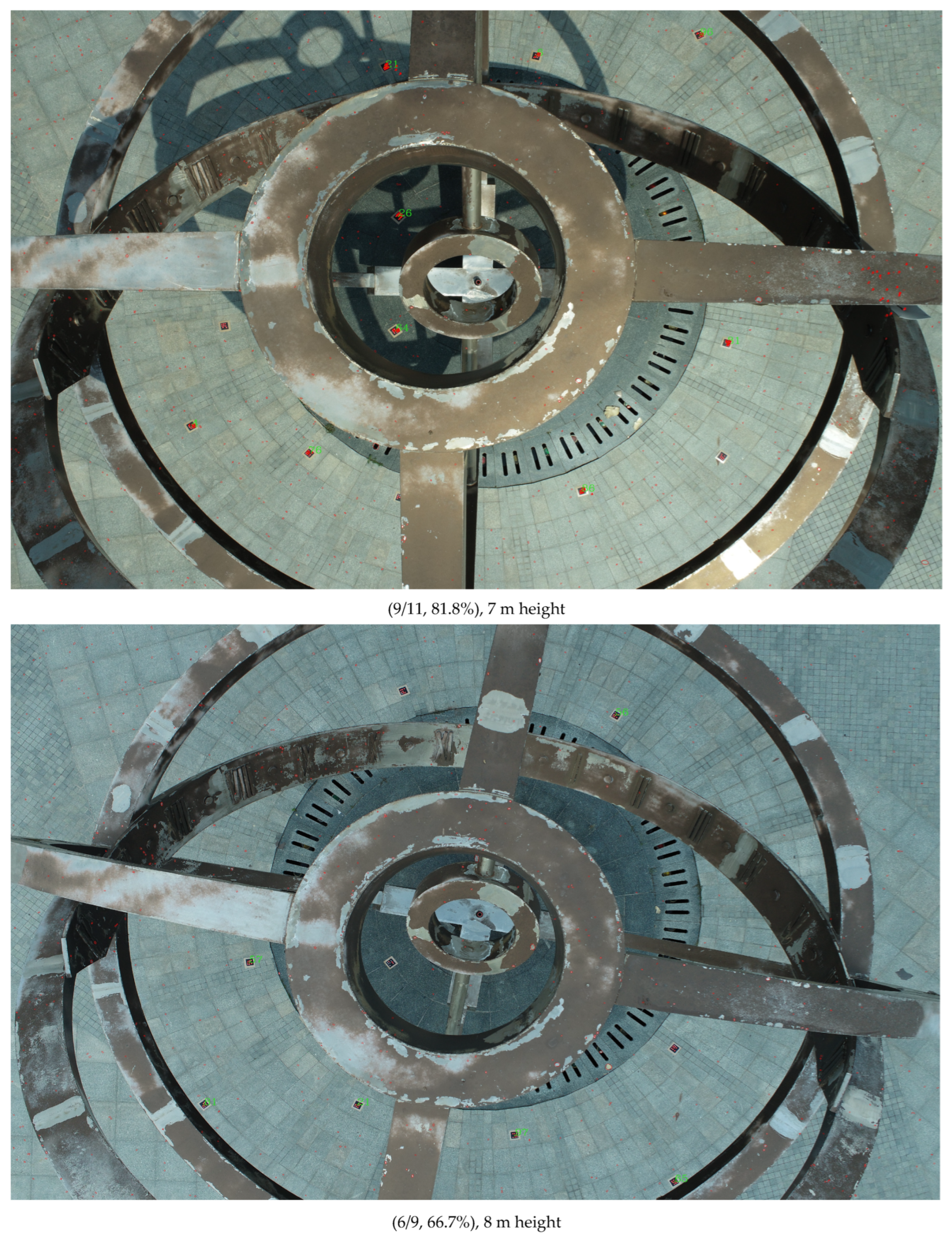
The UAV test, with shooting heights of 4, 7, and 8 m, used nine 12 mm diameter GCTs. The result at a height of 4 m served as a representative result (Figure 14), and the results at the other heights are shown in the Appendix A (Figure A5).
From Figure 14 and Figure A5, and Ref. [16], the improved IPCT obtained the best results which surpassed the results of IPCT and V-STARS. When the height was 7 m and 8 m, the improved IPCT behaved quite satisfactorily with obvious improvement compared to IPCT. In particular, for the image taken at a height of 7 m, we can see that the sunlight was not uniform. For IPCT, the GCTs in the shade could not be identified with the GCTs in the sunlight at the same time, but they were identified successfully here using I-IPCT, which demonstrates the effectiveness of adaptive binarization for challenging illumination. It should be pointed out that, compared with the shooting distance, the size of the 12 mm diameter GCTs was slightly small for the UAV when the shooting height was greater than 4 m. If larger-sized GCTs are adopted, better identifications could be obtained.
As well as the examples of the visible results in the main text and the Appendix A, detailed comparisons of the accurate identification rate between V-STARS, IPCT, and the improved IPCT are listed in Table 1. It is clear that the improved IPCT provides a comprehensive upgrade in its accurate identification rate compared with IPCT. It also performed equally as well as V-STARS on the whole and behaved better than V-STARS for the UAV test.
4. Discussion
The key to the improvement seen with I-IPCT was the adoption of the advanced gray cubic weighted centroid method and the invariance theory of PLDR; therefore, we performed a validation analysis regarding the precision of ellipse-center localization and the robustness of the PLDR. Six milimeter diameter GCTs are the most widely used in common scenarios [14], so this size of GCT was adopted for the experiments and analysis. The validation analysis used every viewing angle with increasing steps ranging from 0 to 80°.
4.1. The Precision of Ellipse-Center Localization
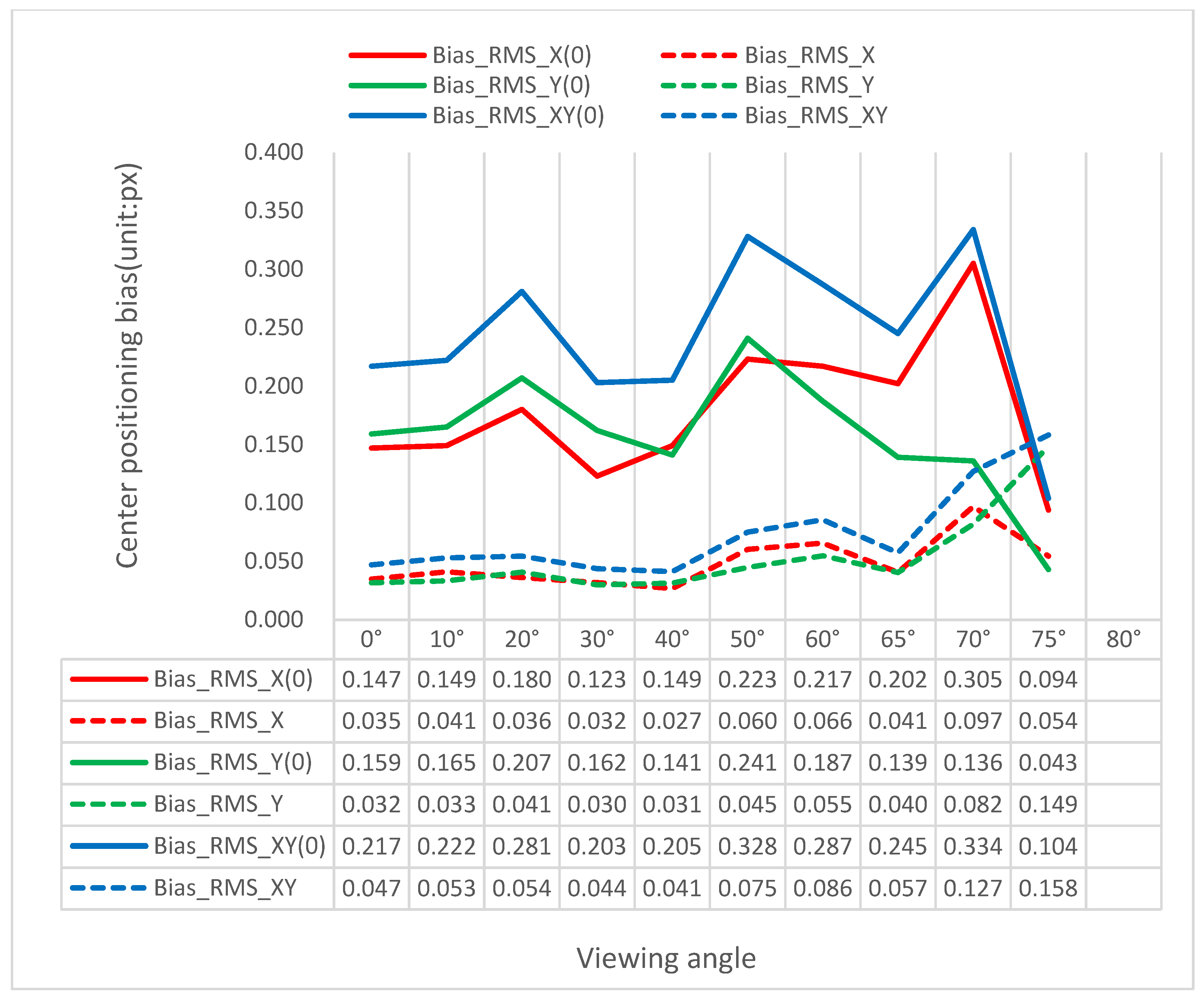
Bias_RMS_X, Bias_RMS_Y, and Bias_RMS_XY represent the root-mean-square error (RMSE) of the biases between the improved IPCT and V-STARS at image coordinates in the X and Y directions and plane, respectively. The detailed information of the localization precision using a viewing angle of 0° can be seen in Table 2. The improved IPCT obtained a high center-localization precision with a plane bias RMSE of 0.047, which is a great breakthrough compared with the plane bias RMSE of 0.217 using IPCT.
The details of the comparisons of IPCT and improved IPCT for center localization precision using different viewing angles are shown in Figure 15. The center positioning precision of IPCT is marked with the symbol (0) with broken lines and the precision of the improved IPCT is presented as solid lines. The RMSE of bias was from approximately 0.04 px to 0.08 px when the viewing angle was less than 65°. The improved IPCT had a worse performance compared to IPCT when the viewing angle was 75° (0.158 vs. 0.104, respectively). The reason is that, as the GCTs were not made of retro-reflective materials and no flash lamp was used, the gray values’ distribution of the round target was not even when the viewing angle was too large. Therefore, the precision of ellipse-center localization by the gray weighted centroid method was worse. On the whole, the improved IPCT can obtain four times better precision. Compared with ellipse fitting, it was obvious that the improved IPCT with the gray cubic weighted centroid algorithm was more suitable for GCT identification and performed more similarly to V-STARS.
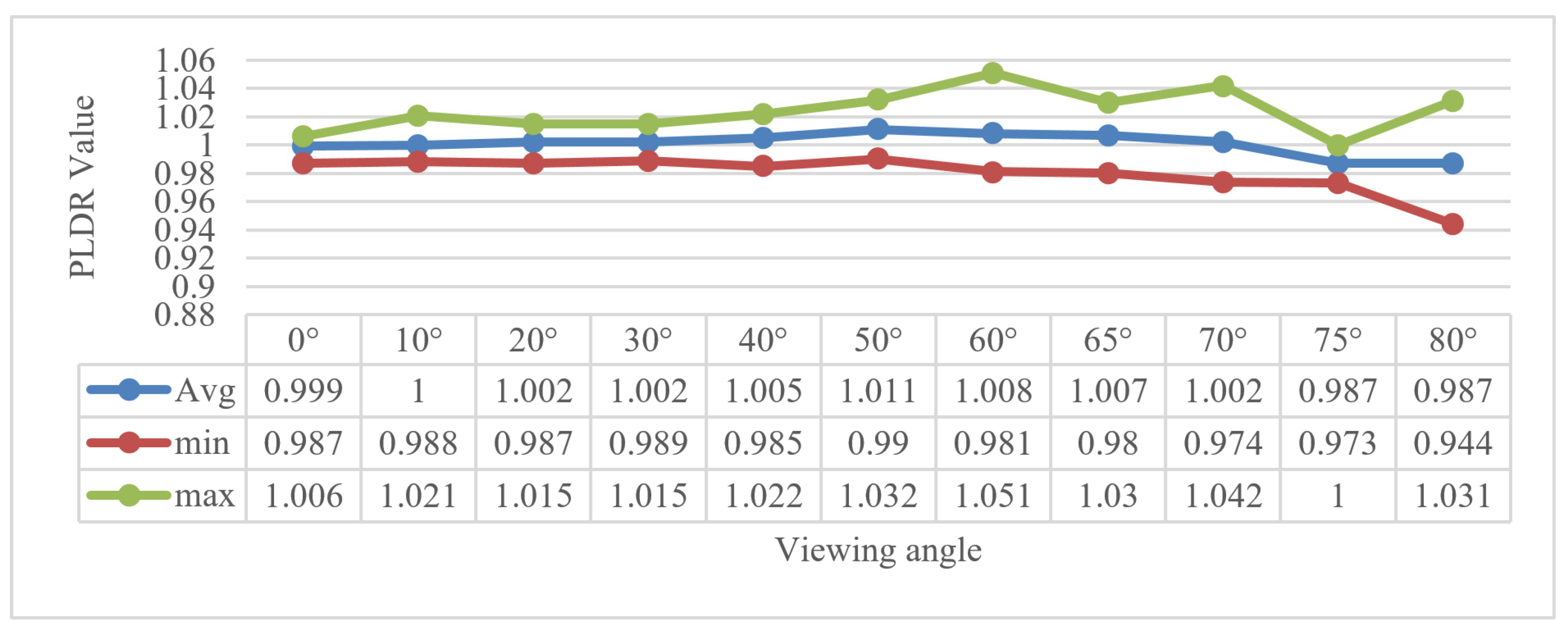
4.2. The Robustness of the PLDR
The variance in the PLDR for template point recognition was used for analysis. We counted the minimum, maximum, and average of the PLDR values. As shown in Figure 16, the average of the PLDR using each viewing angle was close to 1.0. The minimum and maximum PLDR values were 0.944 and 1.051, respectively. The vibration of the PLDR was smaller than 0.06. In addition, the minimum and maximum PLDR values for the outdoor and UAV tests were 0.972 and 0.961 and 1.026 and 1.043, respectively. Thus, the PLDR was very robust and could be adapted for common scenarios when the vibration threshold of the PLDR is set as 0.06.
Next, we provide the statistics on the maximum bias value of the PLDR and the direct positioning for decoding points using different viewing angles (Figure 17). The maximum bias of direct positioning of IPCT was about 0.7 (unit: mm) [16] and the maximum bias of the PLDR was about 0.2 (non-dimensional number). Because the statistic was aimed at the 6 mm diameter GCTs, the maximum bias of direct positioning would be larger than 0.7 mm as the increasing size of the GCTs renders them liable to trigger false decoding. However, the maximum bias of the PLDR was kept invariable as it is irrelevant to the size of the GCTs, and can guarantee the correct decoding. Thus, it is more suitable to use I-IPCT for UAV photogrammetry where large-sized GCTs are needed.
Combined with the PLDR theory and the above results, it can be confirmed that the application of the PLDR is very valid as it is based on the distance ratio constraint, which can be self-adaptive according to the change in image size and image distortion. There is no doubt that it surpasses the distance constraint which should manually tune the parameters according to different application scenarios. On the other hand, the PLDR is very robust as the distance ratio can withstand more error disturbance or uncertainty. As described and tested in the work of Ref. [17], their proposed methods used matched points for line matching, which is rather robust to mismatches from SIFT. They were robust and achieved very good performance even when the percentage of points matching the outlier was as high as 50%. Therefore, the stability of the point–line distance ratio theory could not be easily disturbed by image deformation, and the improved IPCT could achieve parameter-free and more accurate identification.
How can the improved IPCT produce such a good effect? We conclude that the improved IPCT combines three excellent theories together, the gray cubic weighted centroid algorithm, the P2-Invariant, and the invariance of PLDR. Firstly, the gray cubic weighted centroid can provide a precise center positioning for round targets. Secondly, just as the authors of [20,21] mentioned, the P2-Invariant is very stable, scale-invariant, and fast to achieve point registration. Thirdly, based on the work in [16] and [20], the coplanar P2-Invariant assisted by the PLDR can be used to detect template points. Based on the work in Ref. [16] and Ref. [22], the affine transformation assisted by the PLDR can be used to decode a GCT. As the key procedures of the improved IPCT are adaptive, robust, and accurate, it can obtain an excellent identification effect.
4.3. The Precision Validation of 3D Measurement
The high correct-identification rate and the high ellipse-center-positioning precision do not represent the 3D measurement precision. We should evaluate 3D measurement precision by recovering the 3D coordinates of the GCTs. As the commercial photogrammetric system V-STARS remains a closed source [23], the details related to its methods for center positioning and GCT recognition cannot be accessed. However, V-STARS claims to have a typical high measurement precision of 5 µm + 5 µm/m [14,15], and the center-positioning precision is 0.02 px, according to Refs. [14,24,25]. Therefore, the 3D measurement results of V-STARS can be used as the truth. In the following, we go through the whole process of photogrammetry, including performing image matching and bundle adjustment, to help evaluate the center positioning precision and 3D measurement precision further. The same camera, a NIKON D300S, was used to capture three groups of images for these twenty 6 mm sized GCTs. The number of photos for each group were 14, 14, and 15, respectively. Through GCT matching and bundle adjustment, the cameras’ exterior orientations and the 3D coordinates of GCTs were obtained. Taking the first group as an example, the 3D display is shown in Figure 18.
From Figure 19, we can see that the maximum 3D bias was as low as 67 um, and the mean 3D bias was about 20–30 um. The RMS of each group was 25, 25, and 32 um, respectively. For these three tests, the repeated 3D precision was stable and rather good. This indicates the potential for using this method to perform 3D measurements in close-range photogrammetry. In addition, it also reflects the high precision of elliptic-center positioning based on the gray cube weighted centroid method.
In this paper, we used a gray cubic weighted centroid method to obtain the center positions of all points, which may not be the best method to perform center positioning. In future research, we will test other high-precision edge extraction and center positioning methods as mentioned in Ref. [26]. We will also consider a faster ellipse extraction method through learning from Ref. [27] to adapt to fast processing or dynamic scenarios. In addition, another piece of close-range photogrammetric software called AUSTRALIS [28,29] should be considered as a comparison to guide the research.
In the UAV test above, the shooting altitude was 4–8 m. This altitude can be applicable for small objects or research areas, such as heritage buildings [30,31]. However, the shooting altitude is about 50 m or higher for most applications in photogrammetric real-scene 3D-building modeling. Thus, a limitation of the study is that we have not carried out tests with higher shooting altitudes. According to the authors of [14], the size of the GCTs should increase as the shooting distance increases. When the shooting altitude is 80 m, the point’s diameter should be 24 cm and the size of a GCT should be 1.9 m in length and width. As the improved IPCT demands for every GCT to be on a plane, it is not convenient to make such a big GCT or carry such a big flat board for a GCT to be attached. Therefore, the limitations of the improved IPCT are that it is slightly difficult to apply the GCTs in UAV photogrammetry scenes with higher shooting distances, such as 200 m. Our UAV tests in this paper are just a preliminary experiment. We expect other researchers will develop methods with the advantage of using large-sized GCTs and higher shooting altitudes in the future. Furthermore, as our method is not applicable for situations of occlusion and blur, in the future, we will try to identify GCTs through referencing deep learning methods [32].
5. Conclusions
This paper proposed an innovative improved method for GSI-coded target identification based on an adaptive thresh Gaussian binarization, a gray cubic weighted centroid algorithm, and the invariance theory of PLDR, which possesses outstanding performance in binarization, precise ellipse-center localization, and template-point matching and decoding-point matching. According to the data from extensive experiments and analyses of indoor, outdoor, and UAV scenes, the precision of ellipse-center localization by the gray cubic weighted centroid algorithm was very high and the PLDR was very reliable and effective. The proposed identification method achieved a comprehensive improvement compared with the state-of-the-art method and, at the same time, performed comparably to V-STARS or better for the UAV test. The proposed improvement can make identification more precise, accurate, robust, and self-adaptive, which is very important for applications with more complicated scenarios. Additionally, it has presented the potential to be used in 3D high-precision close-range photogrammetry. The contribution of this paper is that it provides an excellent and clear solution for identifying GSI-coded targets; thus, scholars and technicians can carry out research in this area without being constrained by commercial software.
Author Contributions
Conceptualization, Q.W. and Y.S.; formal analysis, Y.L. and Q.W.; investigation, Y.L.; methodology, Q.W.; project administration, X.C.; resources, Q.W. and X.C.; software, Y.L. and Q.W.; supervision, X.C.; validation, Y.L.; visualization, Y.L.; writing—original draft, Y.L. and Q.W.; writing—review and editing, Y.S. and Y.L. All authors have read and agreed to the published version of the manuscript.
Funding
This work was supported by the National Natural Science Foundation of China (Nos. 42001412, 52274169, 52075382) and the Key Research and Development Plan of Guilin (No. 20210214-2).
Data Availability Statement
The experimental data that support the findings of this study are openly available at the following URL/DOI: https://figshare.com/articles/software/GSI_CodedTarget_Identification/20696923 (accessed on 1 April 2023).
Conflicts of Interest
The authors declare no conflict of interest.
Abbreviations
| GSI | Geodetic Systems Inc. |
| V-STARS | Video-simultaneous triangulation and resection system |
| SCT | Schneider circular coded target |
| GCT | GSI-coded target |
| IPCT | Identification for point-distributed coded target |
| I-IPCT | Improved IPCT |
| PLDR | Point–line distance ratio |
| UAV | Unmanned aerial vehicle |
| SIFT | Scale invariant feature transform |
| P2-Invariant | Projective and permutation invariant |
Appendix A
Figure A1.
The identification results of the improved IPCT for middle-sized GCTs using different angles.
Figure A1.
The identification results of the improved IPCT for middle-sized GCTs using different angles.


Figure A2.
The identification results of the improved IPCT for small-sized GCTs.

Figure A3.
The identification results of the improved IPCT for mixed GCTs.

Figure A4.
The identification results of the improved IPCT for outdoor scenes.

Figure A5.
The identification results of the improved IPCT for the UAV.

References
- Wang, Y.M.; Yu, S.Y.; Ren, S.; Cheng, S.; Liu, J.Z. Close-range industrial photogrammetry and application: Review and outlook. AOPC 2020 Opt. Ultra Precis. Manuf. Test. 2020, 11568, 152–162. [Google Scholar]
- Karimi, M.; Zakariyaeinejad, Z.; Sadeghi-Niaraki, A.; Ahmadabadian, A.H. A new method for automatic and accurate coded target recognition in oblique images to improve augmented reality precision. Trans. GIS 2022, 26, 1509–1530. [Google Scholar] [CrossRef]
- Wang, M.; Guo, Y.; Wang QLiu, Y.; Liu, J.; Song, X.; Wang, G.; Zhang, H. A Novel Capacity Expansion and Recognition Acceleration Method for Dot-dispersing Coded Targets in Photogrammetry. Meas. Sci. Technol. 2022, 33, 125016. [Google Scholar] [CrossRef]
- Liu, Y.; Su, X.; Guo, X.; Suo, T.; Yu, Q. A Novel Concentric Circular Coded Target, and Its Positioning and Identifying Method for Vision Measurement under Challenging Conditions. Sensors 2021, 21, 855. [Google Scholar] [CrossRef]
- Chan-Ley, M.; Olague, G.; Altamirano-Gomez, G.E.; Clemente, E. Self-localization of an uncalibrated camera through invariant properties and coded target location. Appl. Opt. 2020, 59, D239–D245. [Google Scholar] [CrossRef]
- Yang, X.; Fang, S.; Kong, B.; Li, Y. Design of a color coded target for vision measurements. Optik 2014, 125, 3727–3732. [Google Scholar] [CrossRef]
- Xia, X.; Zhang, X.; Fayek, S.; Yin, Z. A table method for coded target decoding with application to 3-D reconstruction of soil specimens during triaxial testing. Acta Geotech. 2021, 16, 3779–3791. [Google Scholar] [CrossRef]
- Hurník, J.; Zatočilová, A.; Paloušek, D. Circular coded target system for industrial applications. Mach. Vis. Appl. 2021, 32, 39. [Google Scholar] [CrossRef]
- Mousavi, V.; Khosravi, M.; Ahmadi, M.; Noori, N.; Haghshenas, S.; Hosseininaveh, A.; Varshosaz, M. The performance evaluation of multi-image 3D reconstruction software with different sensors. Measurement 2018, 120, 1–10. [Google Scholar] [CrossRef]
- Schneider, C.T.; Sinnreich, K. Optical 3-D measurement systems for quality control in industry. Int. Arch. Photogramm. Remote Sens. 1993, 29, 56–59. Available online: http://www.isprs.org/proceedings/xxix/congress/part5/56_xxix-part5.pdf (accessed on 26 June 2022).
- Fraser, C.S. Innovations in Automation for Vision Metrology Systems. Photogramm. Rec. 1997, 15, 901–911. [Google Scholar] [CrossRef]
- Available online: https://www.agisoft.com/features/professional-edition/ (accessed on 12 November 2022).
- Liba, N.; Metsoja, K.; Järve, I.; Miljan, J. Making 3D models using close-range photogrammetry: Comparison of cameras and software. Int. Multidiscip. Sci. GeoConf. SGEM 2019, 19, 561–568. [Google Scholar]
- Brown, J.D.; Dold, J. V-STARS—A system for digital industrial photogrammetry. In Optical 3-D Measurement Techniques III; Gruen, A., Kahmen, H.Ž., Eds.; Wichmann Verlag: Heidelberg, Germany, 1995; pp. 12–21. Available online: http://gancell.com/papers/S%20Acceptance%20Test%20Results%20-%20metric%20version.pdf (accessed on 25 August 2022).
- Why V-STARS? Available online: https://www.geodetic.com/v-stars/ (accessed on 27 October 2022).
- Wang, Q.; Liu, Y.; Guo, Y.; Wang, S.; Zhang, Z.; Cui, X.; Zhang, H. A Robust and Effective Identification Method for Point-Distributed Coded Targets in Digital Close-Range Photogrammetry. Remote Sens. 2022, 14, 5377. [Google Scholar] [CrossRef]
- Fan, B.; Wu, F.; Hu, Z. Robust line matching through line–point invariants. Pattern Recognit. 2012, 45, 794–805. [Google Scholar] [CrossRef]
- Wang, Q.; Zhang, W.; Liu, X.; Zhang, Z.; Baig, M.H.A.; Wang, G.; He, L.; Cui, T. Line matching of wide baseline images in an affine projection space. Int. J. Remote Sens. 2019, 41, 632–654. [Google Scholar] [CrossRef]
- Burger, W.; Burge, M.J. Scale-Invariant Feature Transform (SIFT). In Digital Image Processing: An Algorithmic Introduction; Springer International Publishing: Cham, Switzerland, 2022; pp. 709–763. [Google Scholar] [CrossRef]
- Meer, P.; Ramakrishna, S.; Lenz, R. Correspondence of coplanar features through p2-invariant representations. In Proceedings of the Joint European-US Workshop on Applications of Invariance in Computer Vision, Ponta Delgada, Portugal, 9–14 October 1993; Springer: Berlin/Heidelberg, Germany, 1993; pp. 473–492. [Google Scholar]
- Bergamasco, F.; Albarelli, A.; Torsello, A. Pi-Tag: A fast image-space marker design based on projective invariants. Mach. Vis. Appl. 2012, 24, 1295–1310. [Google Scholar] [CrossRef]
- Hattori, S.; Akimoto, K.; Ohnishi, Y.; Miura, S. Semi-automated tunnel measurement by vision metrology using coded-targets. In Modern Tunneling Science and Technology, 1st ed.; Adachi, T., Tateyama, K., Kimura, M., Eds.; Routledge: London, UK, 2017; pp. 285–288. [Google Scholar]
- Tushev, S.; Sukhovilov, B.; Sartasov, E. Robust coded target recognition in adverse light conditions. In Proceedings of the 2018 International Conference on Industrial Engineering, Applications and Manufacturing (ICIEAM), Moscow, Russia, 15–18 May 2018; IEEE: Piscataway, NJ, USA, 2018; pp. 1–6. [Google Scholar]
- Kanatani, K.; Sugaya, Y.; Kanazawa, Y. Ellipse Fitting for Computer Vision: Implementation and Applications. Synth. Lect. Comput. Vis. 2016, 6, 1–141. [Google Scholar] [CrossRef]
- Setan, H.; Ibrahim, M.S. High Precision Digital Close Range Photogrammetric System for Industrial Application Using V-STARS: Some Preliminary Result. In Proceedings of the International Geoinformation Symposium, Bogotá, Colombia, 24–26 September 2003. [Google Scholar]
- Dong, S.; Ma, J.; Su, Z.; Li, C. Robust circular marker localization under non-uniform illuminations based on homomorphic filtering. Measurement 2020, 170, 108700. [Google Scholar] [CrossRef]
- Jia, Q.; Fan, X.; Luo, Z.; Song, L.; Qiu, T. A Fast Ellipse Detector Using Projective Invariant Pruning. IEEE Trans. Image Process. 2017, 26, 3665–3679. [Google Scholar] [CrossRef] [PubMed]
- Fraser, C.S.; Edmundson, K.L. Design and implementation of a computational processing system for off-line digital close-range photogrammetry. ISPRS J. Photogramm. Remote Sens. 2000, 55, 94–104. [Google Scholar] [CrossRef]
- Al-Kharaz, A.A.; Chong, A. Reliability of a close-range photogrammetry technique to measure ankle kinematics during active range of motion in place. Foot 2020, 46, 101763. [Google Scholar] [CrossRef] [PubMed]
- Yang, B.; Ali, F.; Zhou, B.; Li, S.; Yu, Y.; Yang, T.; Liu, X.; Liang, Z.; Zhang, K. A novel approach of efficient 3D reconstruction for real scene using unmanned aerial vehicle oblique photogrammetry with five cameras. Comput. Electr. Eng. 2022, 99, 107804. [Google Scholar] [CrossRef]
- Zhou, T.; Lv, L.; Liu, J.; Wan, J. Application of UAV oblique photography in real scene 3D modeling. ISPRS—Int. Arch. Photogramm. Remote Sens. Spat. Inf. Sci. 2021, 43, 413–418. [Google Scholar] [CrossRef]
- Kniaz, V.V.; Grodzitskiy, L.; Knyaz, V.A. Deep learning for coded target detection. ISPRS—Int. Arch. Photogramm. Remote Sens. Spat. Inf. Sci. 2021, 44, 125–130. [Google Scholar] [CrossRef]
Figure 1.
The construction of a GCT called CODE18.

Figure 2.
The GCT under affine deformation. (a) The designed plane of a GCT and (b) imaging plane of a GCT.
Figure 2.
The GCT under affine deformation. (a) The designed plane of a GCT and (b) imaging plane of a GCT.

Figure 3.
The invariance of the PLDR for line matching.

Figure 4.
The invariance of the PLDR for template point matching. (a) The designed template points and (b) the affined template points.
Figure 4.
The invariance of the PLDR for template point matching. (a) The designed template points and (b) the affined template points.

Figure 5.
The invariance of the PLDR for decoding point matching. (a) The designed decoding points and (b) the affined decoding points.
Figure 5.
The invariance of the PLDR for decoding point matching. (a) The designed decoding points and (b) the affined decoding points.

Figure 6.
The identification process of the improved IPCT.

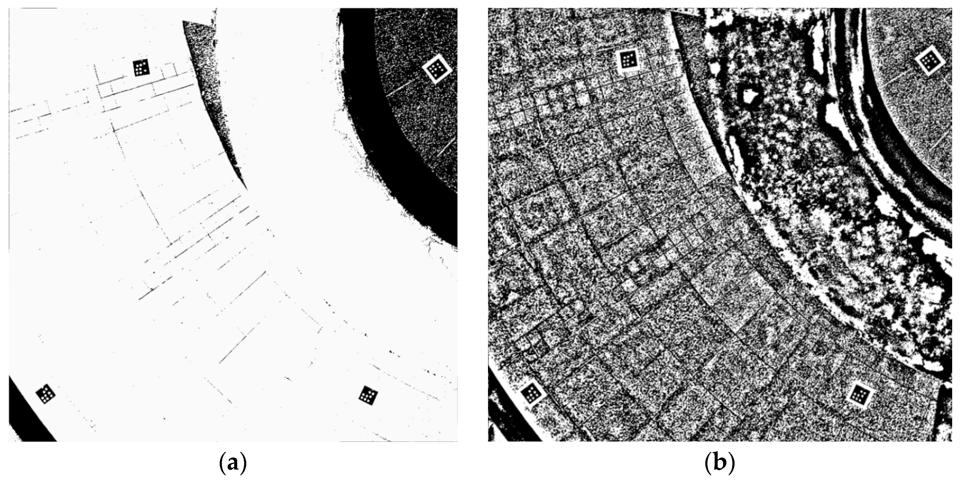
Figure 7.
Comparison of binarization with manual and adaptive methods. (a) The binarization with manual threshold in IPCT and (b) the binarization with adaptive thresh Gaussian in I-IPCT.
Figure 7.
Comparison of binarization with manual and adaptive methods. (a) The binarization with manual threshold in IPCT and (b) the binarization with adaptive thresh Gaussian in I-IPCT.

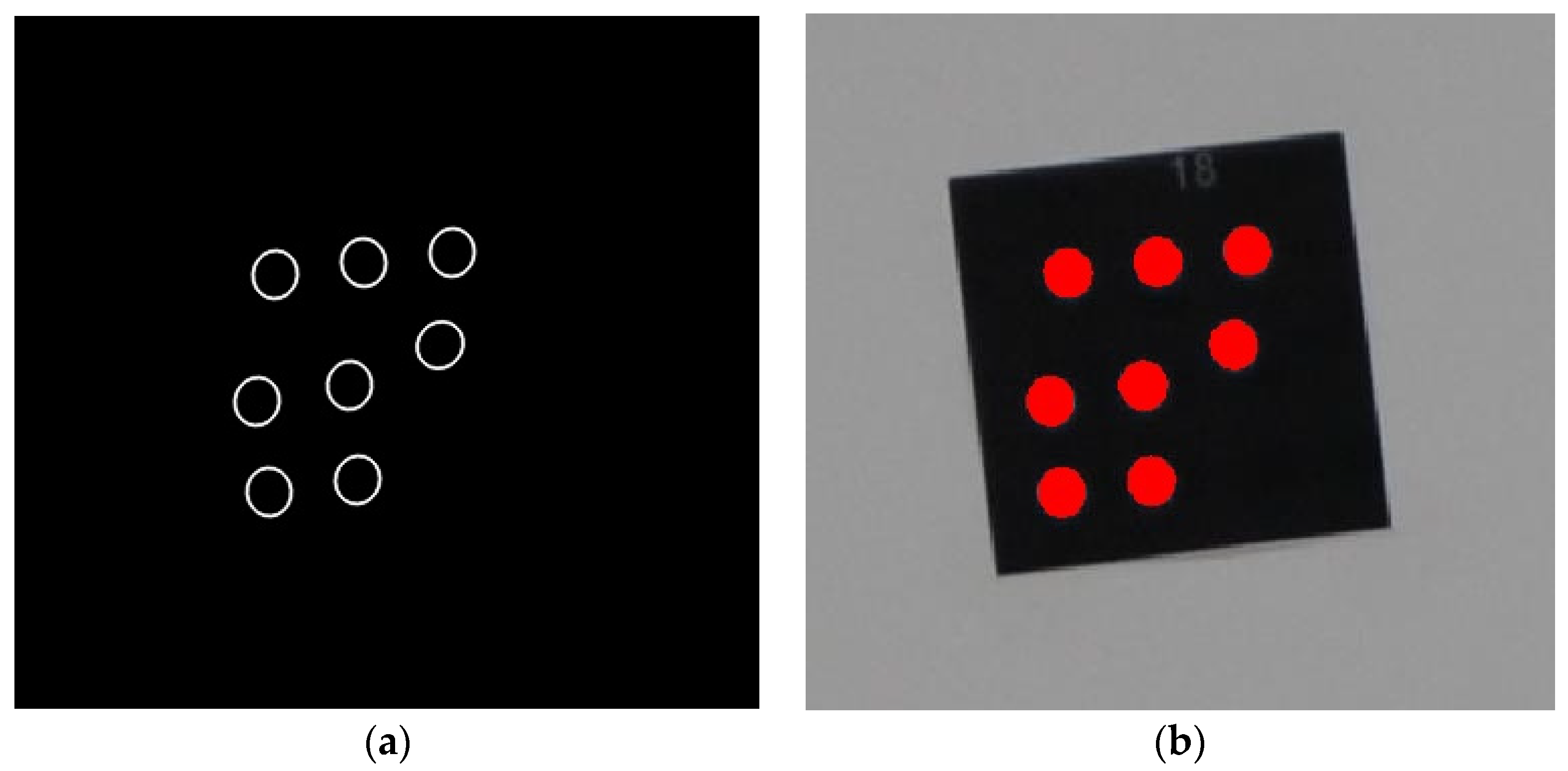
Figure 8.
Comparison of ellipse-center localization between IPCT and I-IPCT. (a) The ellipse-center localization with ellipse fitting and (b) the ellipse-center localization with advanced gray cubic weighted centroid.
Figure 8.
Comparison of ellipse-center localization between IPCT and I-IPCT. (a) The ellipse-center localization with ellipse fitting and (b) the ellipse-center localization with advanced gray cubic weighted centroid.

Figure 9.
The identification results for middle-sized GCTs at viewing angle of 65°.

Figure 10.
The identification results for small-sized GCTs at a viewing angle of 0°.

Figure 11.
The outline shape of CODE21 and CODE83. (a) CODE21 and (b) CODE83.

Figure 12.
The identification results for mixed GCTs with diameters of 3 mm and 6 mm at a viewing angle of 0°.
Figure 12.
The identification results for mixed GCTs with diameters of 3 mm and 6 mm at a viewing angle of 0°.

Figure 13.
The identification results of scene 3 for outdoor GCTs.

Figure 14.
The identification results at a height of 4 m for the UAV.

Figure 15.
Comparison of IPCT and the improved IPCT for precision of center localization using different viewing angles.
Figure 15.
Comparison of IPCT and the improved IPCT for precision of center localization using different viewing angles.

Figure 16.
Statistics of the PLDR values using different viewing angles.

Figure 17.
Comparison of the bias values of the PLDR and direct positioning for decoding points using different viewing angles.
Figure 17.
Comparison of the bias values of the PLDR and direct positioning for decoding points using different viewing angles.

Figure 18.
Cameras’ exterior orientations and 3D coordinates of GCTs of group 1. The 3D coordinates of each GCT calculated by our method was compared with the 3D coordinates of the corresponding GCT through registration. The bias of the 3D coordinates was regarded as the precision of 3D measurement. The 3D coordinates of a total of twenty GCTs were obtained. The biases of group 1, group 2, and group 3 are represented by different colors, as shown in Figure 19.

Figure 19.
Bias of GCTs’ 3D coordinates for the three test groups compared to V-STARS.


Table 1.
Comparisons of V-STARS, IPCT, and I-IPCT in correct identifications.
| Test Cases | Accurate Identification Rate | |||
|---|---|---|---|---|
| V-STARS | IPCT | I-IPCT | ||
| Indoors with medium-sized GCTs | 0° | 100% | 100% | 100% |
| 10° | 100% | 100% | 100% | |
| 20° | 100% | 100% | 100% | |
| 30° | 100% | 100% | 100% | |
| 40° | 100% | 100% | 100% | |
| 50° | 85% | 100% | 100% | |
| 60° | 75% | 100% | 100% | |
| 65° | 100% | 85% | 100% | |
| 70° | 70% | 65% | 75% | |
| 75° | 80% | 5% | 30% | |
| 80° | 50% | 0% | 10% | |
| Indoors with small-sized GCTs | 0° | 100% | 95% | 100% |
| 30° | 100% | 100% | 100% | |
| 60° | 100% | 55% | 75% | |
| Indoors with mixed GCTs | 0° | 100% | 100% | 100% |
| 30° | 100% | 100% | 100% | |
| 60° | 50% | 100% | 100% | |
| Outdoors | Scene 1 | 100% | 100% | 100% |
| Scene 2 | 100% | 100% | 100% | |
| Scene 3 | 90.9% | 90.9% | 100% | |
| UAV | 4 m | 75% | 100% | 100% |
| 7 m | 81.8% | 72.7% | 81.8% | |
| 8 m | 55.6% | 44.4% | 66.7% | |
Table 2.
The coordinates and bias of center localization compared with V-STARS using a viewing angle of 0°.
Table 2.
The coordinates and bias of center localization compared with V-STARS using a viewing angle of 0°.
| Coding | Center Positioning Coordinate (x,y) (Unit: px) | Positioning Bias (Unit: px) | |||
|---|---|---|---|---|---|
| Serial Number | V-STARS | The Improved IPCT | |||
| 3 | (2950.418,2222.000) | (2950.430,2222.032) | −0.012 | −0.032 | 0.034 |
| 8 | (1266.945,670.800) | (1266.910,670.769) | 0.035 | 0.031 | 0.047 |
| 13 | (1116.764,1912.218) | (1116.745,1912.251) | 0.019 | −0.033 | 0.038 |
| 18 | (2365.036,1127.382) | (2365.085,1127.405) | −0.049 | −0.023 | 0.054 |
| 23 | (3019.909,412.727) | (3019.936,412.734) | −0.027 | −0.007 | 0.028 |
| 28 | (1307.745,2373.909) | (1307.781,2373.976) | −0.036 | −0.067 | 0.076 |
| 33 | (1650.145,1127.909) | (1650.124,1127.886) | 0.021 | 0.023 | 0.031 |
| 38 | (2470.600,1883.091) | (2470.627,1883.129) | −0.027 | −0.038 | 0.047 |
| 43 | (2463.727,401.327) | (2463.748,401.324) | −0.021 | 0.003 | 0.021 |
| 48 | (3299.764,1770.691) | (3299.834,1770.704) | −0.070 | −0.013 | 0.071 |
| 53 | (3372.509,1097.691) | (3372.512,1097.681) | −0.003 | 0.010 | 0.010 |
| 58 | (2002.491,686.655) | (2002.503,686.621) | −0.012 | 0.034 | 0.036 |
| 63 | (2165.400,2388.618) | (2165.397,2388.648) | 0.003 | −0.030 | 0.030 |
| 68 | (2833.673,856.636) | (2833.734,856.617) | −0.061 | 0.019 | 0.064 |
| 73 | (1645.036,253.364) | (1645.045,253.319) | −0.009 | 0.045 | 0.046 |
| 78 | (2885.182,1407.964) | (2885.242,1407.954) | −0.060 | 0.010 | 0.061 |
| 83 | (2052.600,1632.600) | (2052.636,1632.609) | −0.036 | −0.009 | 0.037 |
| 88 | (1510.909,1611.400) | (1510.934,1611.455) | −0.025 | −0.055 | 0.060 |
| 93 | (1728.127,2075.018) | (1728.090,2075.064) | 0.037 | −0.046 | 0.059 |
| 98 | (1108.182,1199.545) | (1108.207,1199.545) | −0.025 | 0.000 | 0.025 |
| RMSE | 0.035 | 0.032 | 0.047 | ||
Disclaimer/Publisher’s Note: The statements, opinions and data contained in all publications are solely those of the individual author(s) and contributor(s) and not of MDPI and/or the editor(s). MDPI and/or the editor(s) disclaim responsibility for any injury to people or property resulting from any ideas, methods, instructions or products referred to in the content. |
© 2023 by the authors. Licensee MDPI, Basel, Switzerland. This article is an open access article distributed under the terms and conditions of the Creative Commons Attribution (CC BY) license (https://creativecommons.org/licenses/by/4.0/).
Share and Cite
MDPI and ACS Style
Liu, Y.; Cui, X.; Wang, Q.; Sun, Y. Improved Identification for Point-Distributed Coded Targets with Self-Adaption and High Accuracy in Photogrammetry. Remote Sens. 2023, 15, 2859. https://doi.org/10.3390/rs15112859
AMA Style
Liu Y, Cui X, Wang Q, Sun Y. Improved Identification for Point-Distributed Coded Targets with Self-Adaption and High Accuracy in Photogrammetry. Remote Sensing. 2023; 15(11):2859. https://doi.org/10.3390/rs15112859
Chicago/Turabian StyleLiu, Yang, Ximin Cui, Qiang Wang, and Yanbiao Sun. 2023. "Improved Identification for Point-Distributed Coded Targets with Self-Adaption and High Accuracy in Photogrammetry" Remote Sensing 15, no. 11: 2859. https://doi.org/10.3390/rs15112859
Note that from the first issue of 2016, this journal uses article numbers instead of page numbers. See further details here.