
Impact of Global Warming on Tropical Cyclone Track and Intensity: A Numerical Investigation
by
Zhihao Feng
1,
Jian Shi
1,
Yuan Sun
2,*,
Wei Zhong
2,
Yixuan Shen
3,
Shuo Lv
4,
Yao Yao
2,5 and
Liang Zhao
2 1
College of Meteorology and Oceanography, National University of Defense Technology, Changsha 410073, China
2
College of Advanced Interdisciplinary Studies, National University of Defense Technology, Nanjing 211100, China
3
PLA Troop 32033, Haikou 570100, China
4
PLA Troop 31204, Guangzhou 510000, China
5
School of Atmospheric Sciences, Nanjing University, Nanjing 210093, China
*
Author to whom correspondence should be addressed.
Remote Sens. 2023, 15(11), 2763; https://doi.org/10.3390/rs15112763
Submission received: 3 May 2023
/
Accepted: 24 May 2023
/
Published: 25 May 2023
(This article belongs to the Topic Numerical Models and Weather Extreme Events)
Abstract
:Despite numerous studies, the impact of global warming on the tropical cyclone (TC) track and intensity by reasons of data inhomogeneity in remote sensing and large natural variability over a relatively short period of observation is still controversial. Three carbon-emission sensitivity experiments are conducted to investigate how TC track and intensity respond to changes in the oceanic and atmospheric environment under global warming. The results show a high sensitivity of the simulated TC track and intensity to global warming. On one hand, with increase in carbon emissions, the western Pacific subtropical high expands notably, increasing the poleward steering flow and eventually leading to a poleward shift of TC. On the other hand, the underlying sea-surface temperature and surface-entropy flux increase and, thus, favor the convections near the eyewall. Moreover, the TC structure becomes more upright, which is closely related to the larger pressure gradient near the eyewall. As a result, TC intensity increases with carbon emissions. However, this increase is notably smaller than the maximum potential intensity theory as the TC intensity can reach a threshold if carbon emission still increases in the future. The involved mechanisms on the changes of TC track and intensity are also revealed.
1. Introduction
Tropical cyclones (TCs) can be catastrophic to our planet Earth [1,2]. TC-related disasters are commonly found in and around the western North Pacific (WNP) and North Atlantic [3,4,5,6]. Previous studies showed that global warming can be a major factor in the changes of TC activity (increase in frequency and destructiveness, and change of track) [3,7,8,9,10,11,12]. However, it is still a highly controversial issue. Under the condition of global warming, the change of WNP TC activities and the involved physical mechanisms are not only hot topics in science but also of great public concern; thus, they need to be carefully investigated.
Under the condition of global warming, ocean temperature (e.g., SST) increases, but the atmospheric circulation (e.g., western Pacific subtropical high, or WPSH) also changes significantly [13,14,15]. These changes can greatly contribute to changes in TC track and intensity. For example, global warming tends to have great influence on TC track. Possibly due to the tropical expansion, the WNP TCs systematically migrated poleward in the past decades [16,17,18]. Moreover, the WPSH is a major factor in the East Asian monsoon system, due to which the large-scale forcing connected with WPSH plays a determinant role in the East Asian monsoon climate and the TC track over the WNP [19,20]. As indicated by Sun et al. [21], the WPSH’s main body is likely to move to the east, and the TC has a tendency to turn poleward earlier under global warming.
Despite the fact that global warming is assumed to contribute greatly to TC intensity, the influence of global warming falls far short of our expectation. While low-level sensible and latent heat fluxes provide the main energy input for TCs, SST is a crucial factor that determines the formation and intensification of TCs [22,23,24,25,26,27]. According to the MPI theory [18], TC intensity can increase by 5.36 m s−1 and 15.6 hPa with 1 °C increase in SST. However, not robust results support the TC intensity enhancement in the past several decades based on observations. This indicates that following the ongoing global warming, there must be some other factors partly balancing TC intensity enhancement effect caused by the SST increase. In fact, global warming includes not only the increase in ocean temperature (e.g., SST) but also the change of atmospheric circulation (e.g., 500-hPa geopotential height) [13,14]. A previous study indicated that ocean warming (e.g., SST increase) can cause the temperature of the upper troposphere to rise [14]. These changes in global warming may influence TC activities in different intensity [28]. According to the Carnot cycle theory [22,29], TC intensity is closely linked to the SST/upper tropospheric temperature gap. Therefore, under global warming, while the increase in SST favors the increase in TC intensity, the changes of atmospheric dynamic structure and atmospheric thermal structure (e.g., increase in upper tropospheric temperature) tend to weaken TC intensity. Unfortunately, the latter changes have often been underestimated or ignored in published studies.
With the aim of evaluating the impact of global warming on TC over the WNP, we investigated the TC track and intensity from 1980 to 2021 based on the IBTrACS dataset and shed new light on this issue by using a suite of idealized global warming experiments that include different global warming environments. We focused on the physical processes involved in how global warming influences TC track and intensity. In addition, to study the impact of global warming on TC track and intensity over the WNP, we made multiple experimental attempts. We conducted simulation of three experiments under different carbon emissions by using the Coupled Ocean Atmosphere Wave Sediment Transport (COAWST) modeling system. The paper is structured in the following manner. Data sources and model configuration are described in Section 2. Results of TC track and intensity variation trend and physical mechanism analysis are detailed in Section 3. Conclusions and discussion are summarized in Section 4.
2. Data and Methods
2.1. IBTrACS Dataset
The TC data used in this study are data of all numbered TCs and all unnumbered influential TCs over the WNP recorded in the IBTrACS dataset. IBTrACS is a global archive of TC best track data that uses remote sensing data such as satellite imagery, microwave and infrared imagery, scatterometry, and other data sources to determine the best track of TCs [16]. The remote sensing data help to improve the accuracy of the analysis and enable researchers to study changes in TC behavior over time. The IBTrACS dataset has a temporal resolution of 6 h and records the longitudes and latitudes, the central minimum pressure, and the 2 min average near-center maximum wind speed of the TCs at UTC 00:00, 06:00, 12:00, and 18:00. In this paper, the data are mainly used to obtain information such as TC position and intensity.
The IBTrACS dataset assimilates many ground-based remote sensing data and satellite data. As most of the geostationary satellites (an important tool for studying TC activities) did not appear until around 1980, the time range of the IBTrACS dataset is from 1980 to 2021 to ensure data accuracy.
2.2. EC-Earth3 Model of CMIP6
The data on the 6th phase of the Coupled Model Intercomparison Project (CMIP6) are available online (https://pcmdi.llnl.gov/CMIP6/ (accessed on 1 May 2023)). Among the CMIP6 models, one is developed by the European EC-Earth consortium with Swedish Meteorological and Hydrological Institute (SMHI) as coordinating partner, namely EC-Earth3. As the EC-Earth3 model performs well in TC simulation [30], we select it for our sensitivity experiments. The temporal frequency of atmosphere elements (e.g., surface wind, surface air pressure, air temperature) and ocean elements (e.g., sea-surface height, salinity, currents) is a monthly average.
2.3. Experimental Design of Historical, SSP245, and SSP585 Experiments
The EC-Earth3 model includes a historical scenario and two future scenarios of carbon emission increases. Specifically, the historical scenario run (Historical) is a historical climate simulation which started in the 19th century, from 1840 to 2014, and was driven by various external forces based on observations. For future scenarios, the scenario comparison plan (scenarioMPI) in the CMIP6 uses the combination of shared socio-economic pathways (SSPs) and representative concentration pathways (RCPs). For the future scenarios, SSP245 and SSP585 are selected as prediction scenarios based on specific CO2 atmospheric concentrations. SSP245 (SSP585) is a future scenario based on SSP2 (SSP5), and the global forcing path roughly follows RCP4.5 (RCP8.5), namely moderate radiative forcing (high radiation forcing) at the end of this century. The simulation of the SSP245 and SSP585 scenarios in EC-Earth3 model is from 2015 to 2100.
The historical (SSP245/SSP585) scenario data of 30 years, i.e., 1985–2014 (2071–2100), is used to construct the mean climate state as the initial conditions and boundary conditions of COAWST model in the Historical (SSP245/SSP585) experiment. We used data from multiple variables (e.g., the absolute potential vorticity, vertical wind shear, and relative humidity) to calculate the genesis potential index (GPI) of years and each month. We divide the months GPI in the total GPI to obtain the weights of each month and weighted average variable field. The weighted average variable field is used as the initial field and boundary conditions to drive the COAWST model for TC simulation. Note that the model runs for 7 days in all three experiments, and TC is experienced through its full life cycle.
2.4. COAWST Modeling System
In our study, the coupled ocean–atmosphere–wave–sediment transport (COAWST) modeling system, which includes three model components—an atmospheric model, an ocean model, and a wave model—is utilized [31]. The Model Coupling Toolkit (MCT) is used in the COAWST modeling system to exchange data among the model components (i.e., WRF, ROMS, and SWAN) [31,32,33,34]. The Spherical Coordinate Remapping Interpolation Package (SCRIP) in MCT develops the interpolation weights to pass variables from one component to another [35]. In this study, SCRIP is used to convert between the WRF and collocated ROMS and SWAN domains. To interpolate the nested WRF grids to ROMS and SWAN grids (and vice versa), SCRIP calculates the interpolation weight for each location, and then MCT determines the interpolation weight and location between the nested WRF domain and ROMS/SWAN grid.
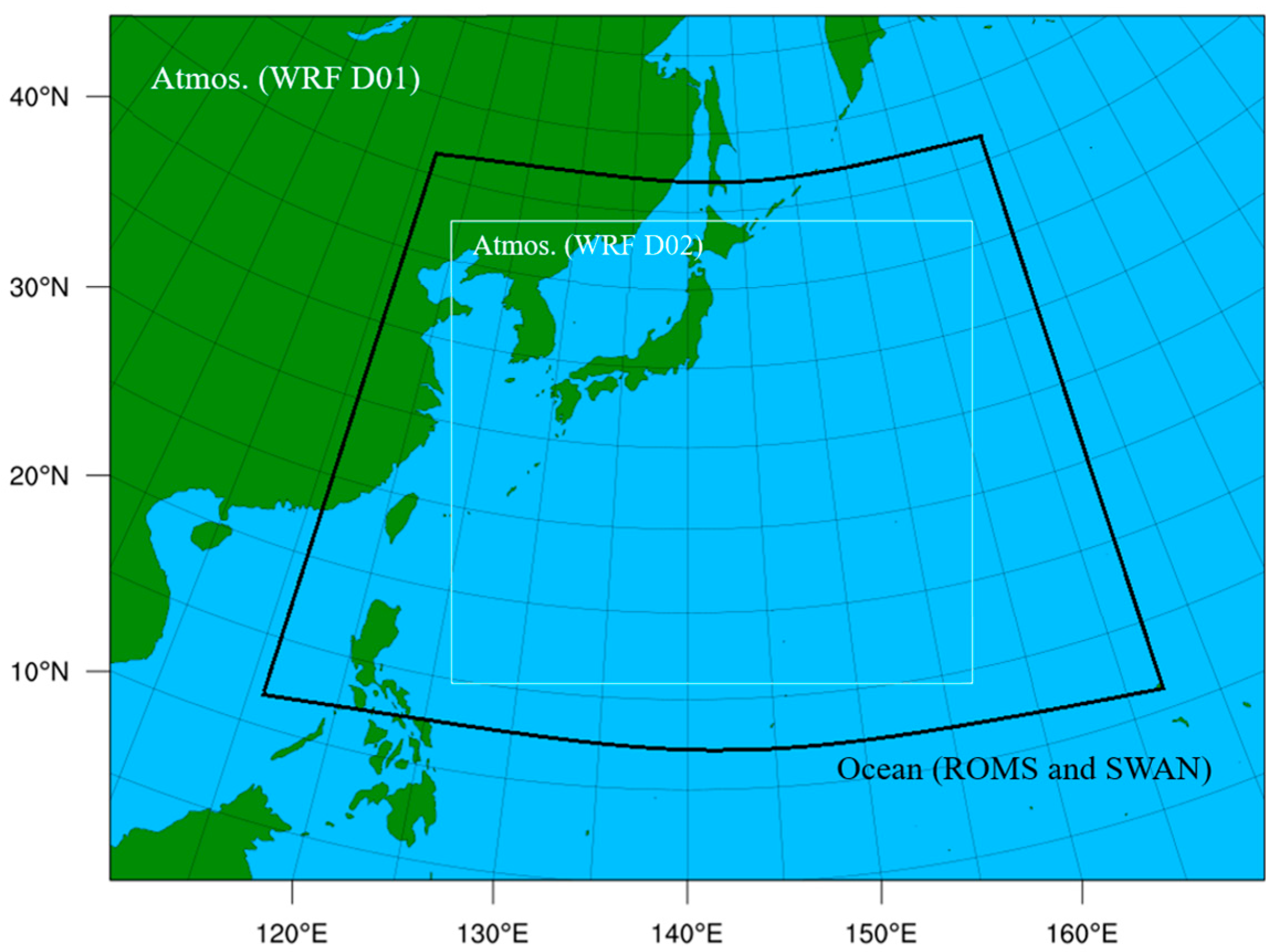
The atmospheric model Weather Research and Forecasting (WRF), as the atmospheric part of the coupled modeling system, is set up as a non-hydrostatic model with full compressibility that offers plentiful physical parameterization schemes [36]. The WRF Domain 1 (Figure 1) is selected to encompass the ROMS and SWAN Domain at a grid spacing of 20 km with 400 × 300 grid points and 60 s time step. A smaller grid, Domain 2, with a grid spacing of 4 km (900 × 800 grid points) and a time step of 20 s is used. Both grids have 41 vertical layers that follow the hybrid-sigma coordinate. The following model physics are used in WRF: WSM 6-class graupel scheme for cumulus from Hong and Lim [37]; Tiedtke cumulus parameterization from Tiedtke [38]; RRTMG scheme for shortwave and longwave physics [39]; planetary boundary layer scheme of the Hong YSU scheme [40]; revised MM5 Monin–Obukhov scheme for surface layer physics [36]; and land surface physics from the Unified Noah Land Surface model [41].
The Regional Ocean Modeling System (ROMS) is the ocean model component of the COAWST system. It is a three-dimensional numerical model that follows the free surface terrain and uses the hydrostatic and Boussinesq assumptions to solve the Reynolds-Averaged Navier-Stokes equations [42,43]. As an independent model, the ROMS, with a range of advection schemes, turbulence models, lateral boundary conditions, as well as surface and bottom boundary layer schemes, can run fully parallelly. To resolve the surface conditions provided by the WRF model with an improved resolution than those provided by a global model, the ocean domain is located somewhat inside of the WRF Domain 1 (Figure 1). In this study, a total of 25 vertical sigma levels with a terrain-following configuration to provide a finer vertical grid near the ocean surface are used in the ROMS model with a resolution of 5 km (990 × 780 grid points). A 30 s baroclinic time step is used. Furthermore, Tides data come from the TPXO9 model, and the 15 tidal constituents derived from TPXO9 at the open boundaries are included [44,45].
The Simulating Wave Nearshore (SWAN) model is used as the wave model component in COAWST system. As a third-generation wave model, the SWAN is based on the wave action equation with sinks and sources [46]. It is able to capture and track the generation and propagation of wind waves with numerous physical schemes, including shoaling, diffraction, refraction, and wave–wave interaction. The grid of SWAN is the same as that of ROMS (Figure 1). Wave energy loss due to bottom friction is parameterized using the formulation proposed by Madsen et al. [47]. The growth of wind waves is generated using the Komen and Hasselmann formulation [48]. The atmosphere boundary conditions of SWAN are provided by the WRF model, and the ocean boundary conditions are provided by the ROMS model.
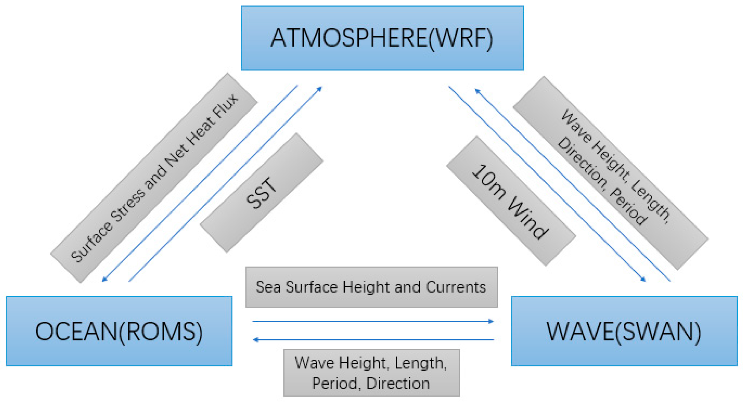
In the coupling process, fields among the coupled model components are exchanged every 15 min. The coupled variables (i.e., surface stress, SST, wave height) are shown in Figure 2. WRF model mainly provides 10 m wind to drive wind–wave generation in SWAN and surface stress and net heat flux to ROMS. SST are the most important variables from ROMS and are passed onto WRF. Sea-surface height is derived from ROMS to SWAN to solve bottom friction and depth-limited breaking. Wave parameters (e.g., wave height, length, direction, and period) are derived from SWAN and passed on to WRF and ROMS.
2.5. Bogus Scheme
The initialization of TC in the numerical model has been a long-standing challenge. TC intensity is not well represented in the initial condition, which is interpolated from global reanalysis data, and may not have the resolution needed to resolve the real TC structure. To improve simulation accuracy of TC intensity and reduce the spin-up time before reproducing similar TC intensity, the WRF provides a Bogus scheme to build the initial vortex at the model start time [49]. By defining the longitude and latitude, the maximum wind speed at 10 m height in the center, the radius of the maximum wind speed, and other information, a new Rankine vortex is implanted into the initial condition of the model. At present, a large number of experimental results show that the accuracy of TC simulation can be effectively improved by implanting TC vortices into the initial field of model [50,51]. In this study, we use the Bogus scheme to obtain simulation results of TC in different carbon emission backgrounds.
3. Results and Physical Mechanisms
3.1. TC Track and Intensity Changes during 1980–2021
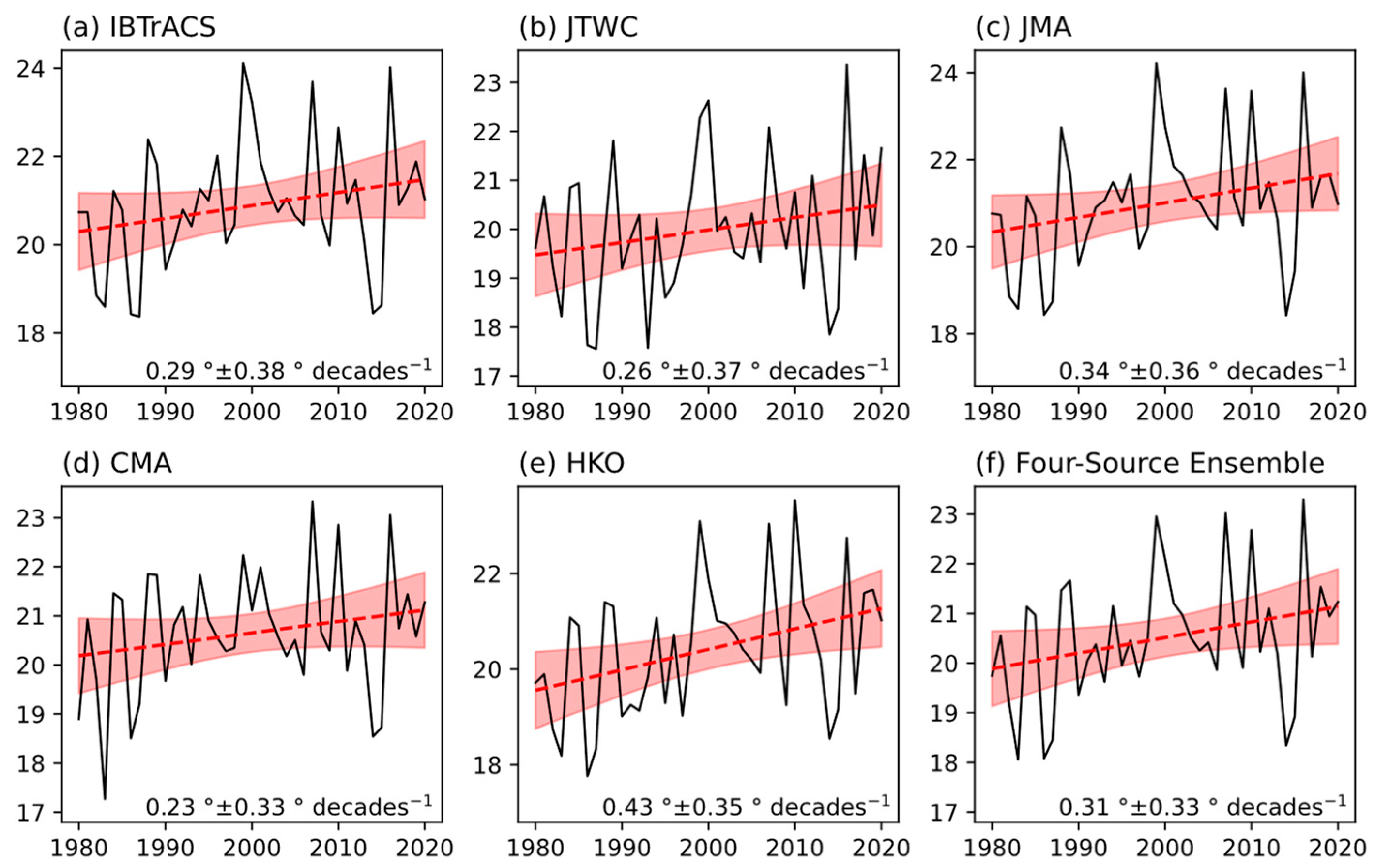
Based on the IBTrACS dataset, we investigated the changes of TC track and intensity in the WNP from 1980 to 2021. The TC latitude showed an obvious poleward migration, which is consistent with the previous studies (Figure 3a) [16,17]. Figure 3b–f show the results from different institutions (e.g., JTWC, JAM, CMA, HKO, and Four-Source Ensemble), all of which proved the existence of a poleward migration, and the result from HKO passed the 95% significance test.
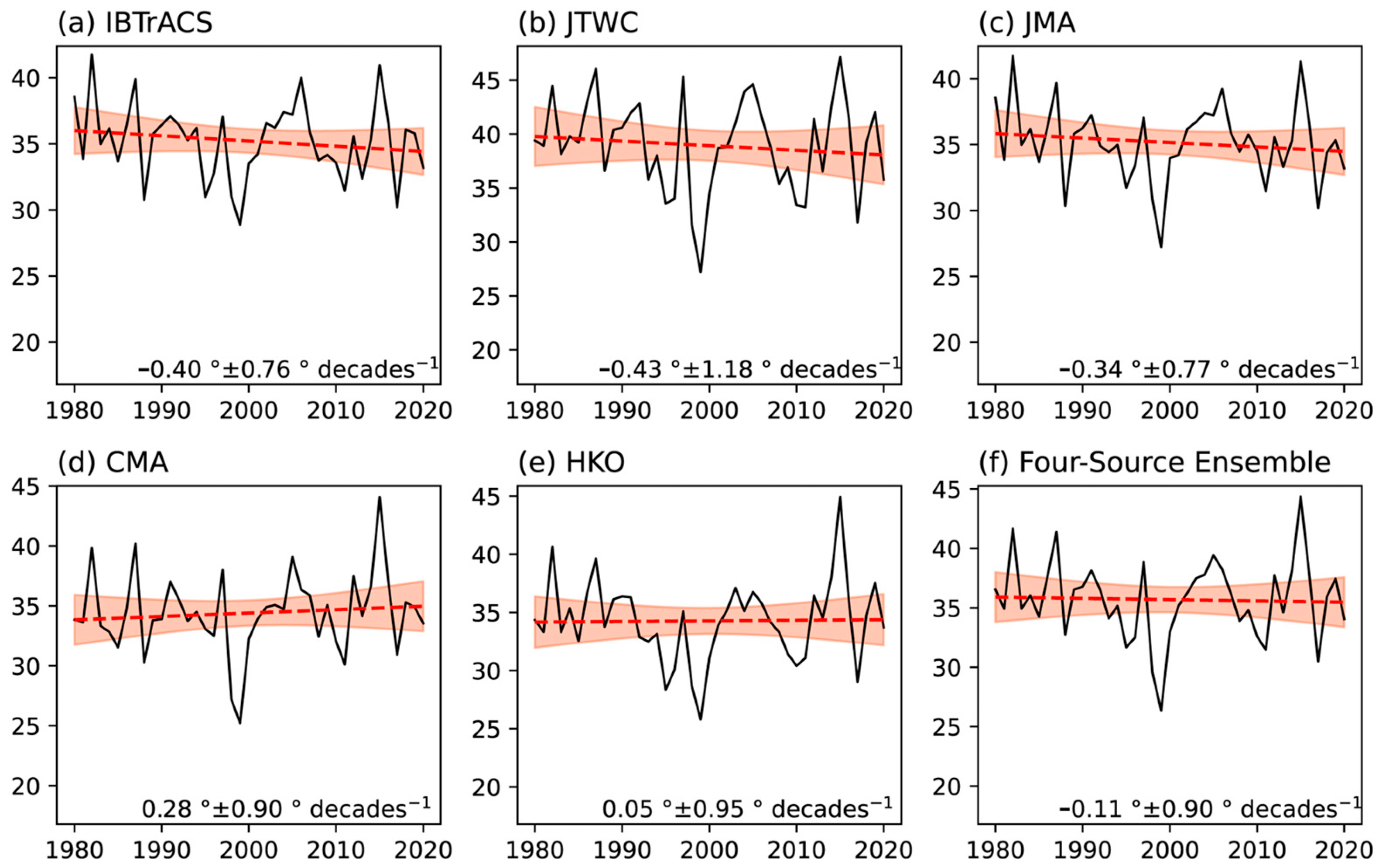
As for TC intensity, the different data presented both increasing and decreasing results, and they all failed the 95% significance test (Figure 4). However, since the variation of TC intensity shows a clear interannual oscillation, many studies suggest that this may be related to the large natural variability in the WNP (e.g., ENSO, IPO and PDO) [52,53,54].
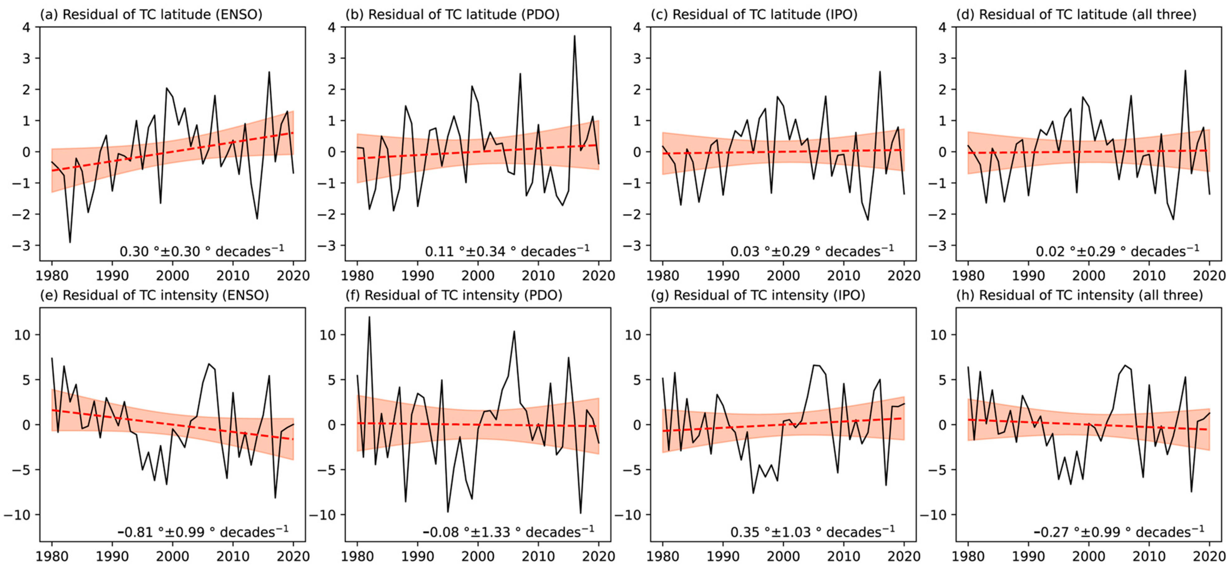
According to Kossin et al. [16], we calculated the residuals of annual mean TC latitude and TC intensity minus ENSO, POD, and IPO indices to exclude the effect of large natural variability. After the effect of large natural variability is removed, there is no obvious trend in either TC track or TC intensity (Figure 5), which is different from Figure 3 and Figure 4, especially for TC track. This indicates the important role of the natural variability in determining TC track.
However, using only 42 years of TC data to investigate the influence of global warming on TC activities would be somewhat inadequate because of data inhomogeneity over a relatively short period of observation. To overcome data inhomogeneity in remote sensing (beginning from 1980) and avoid the large natural variability, we use the COAWST model and CMIP6 data to explore the changes in TC track and intensity in the global warming context and the physical mechanisms behind them, based on three carbon-emission contexts (i.e., Historical, SSP245, and SSP585) in this study.
3.2. Sea-Surface Temperature
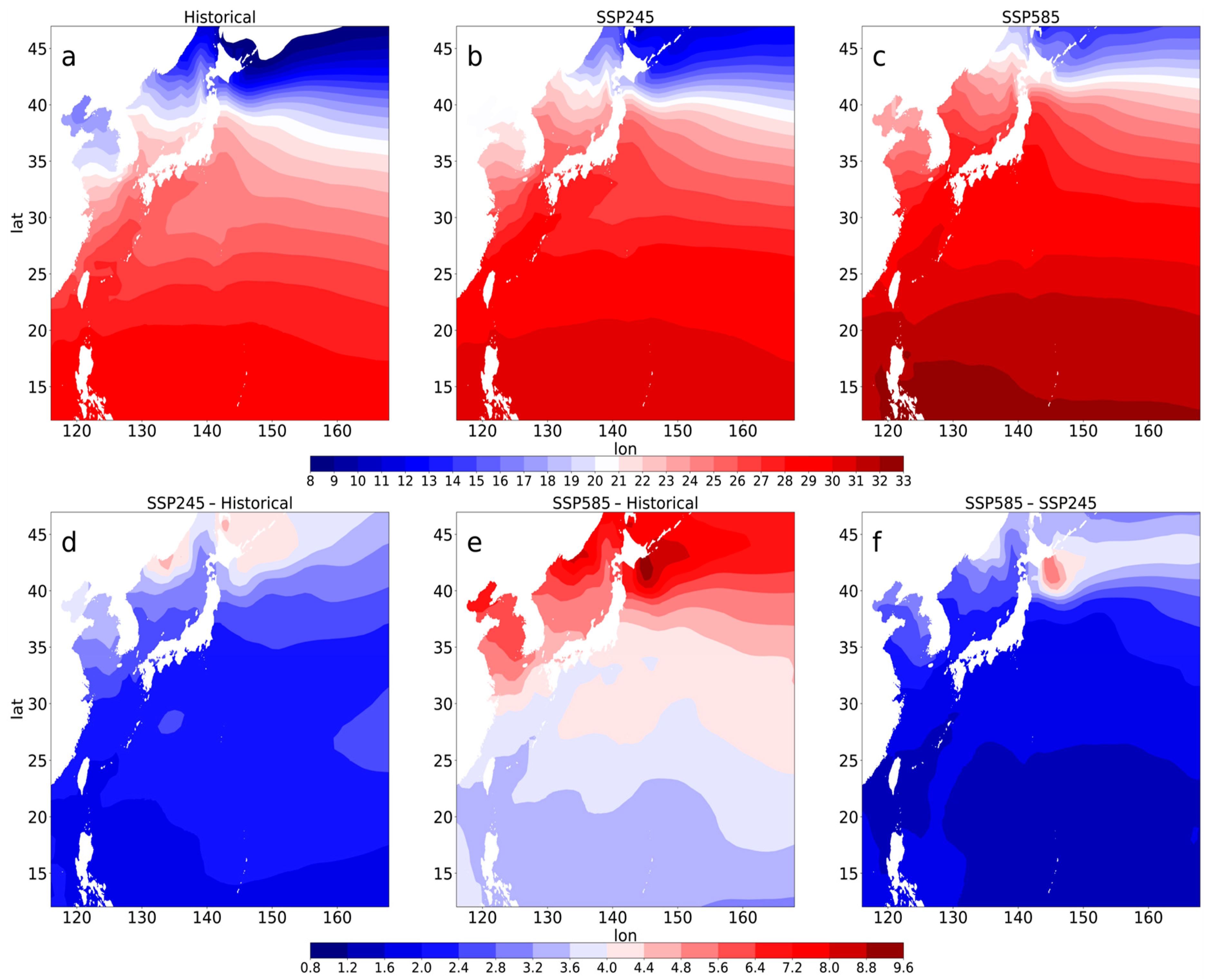
SST is not only sensitive to global warming but also a key factor to TC track and intensity, which makes it necessary to analyze the response of SST to global warming. Figure 6 shows the spatial distributions of climate mean SST in three carbon emission experiments within the ocean domain. It is obvious that the SST ascends in sequence of Historical, SSP245, and SSP585 (Figure 6a–c). To further investigate the regional distribution characteristics of SST increase, we plot Figure 6d–f and find that following the increase in carbon emission, the SST under the TC increases nonuniformly, namely the SST increase in the higher latitude region is much larger than that in the lower latitude region, which agrees with the results of Wu and Chan [55].
3.3. TC Track
To effectively examine the reaction of TC activity to global warming, the model configuration including Bogus scheme is identical in different carbon emission experiments. Figure 7 shows the simulated TC tracks in the three carbon emission experiments. All experiments have similar TC tracks during early stage of TC. However, obvious differences appear after 24 h. Following the increase in carbon emission, the simulated TC migrated poleward early, causing the TC track to shift poleward. This agrees well with the findings in the published works [14,16,17,18], which suggest the high sensitivity of the simulated TC track to the change of underlying SST, namely the tendency of a poleward shift with global warming.
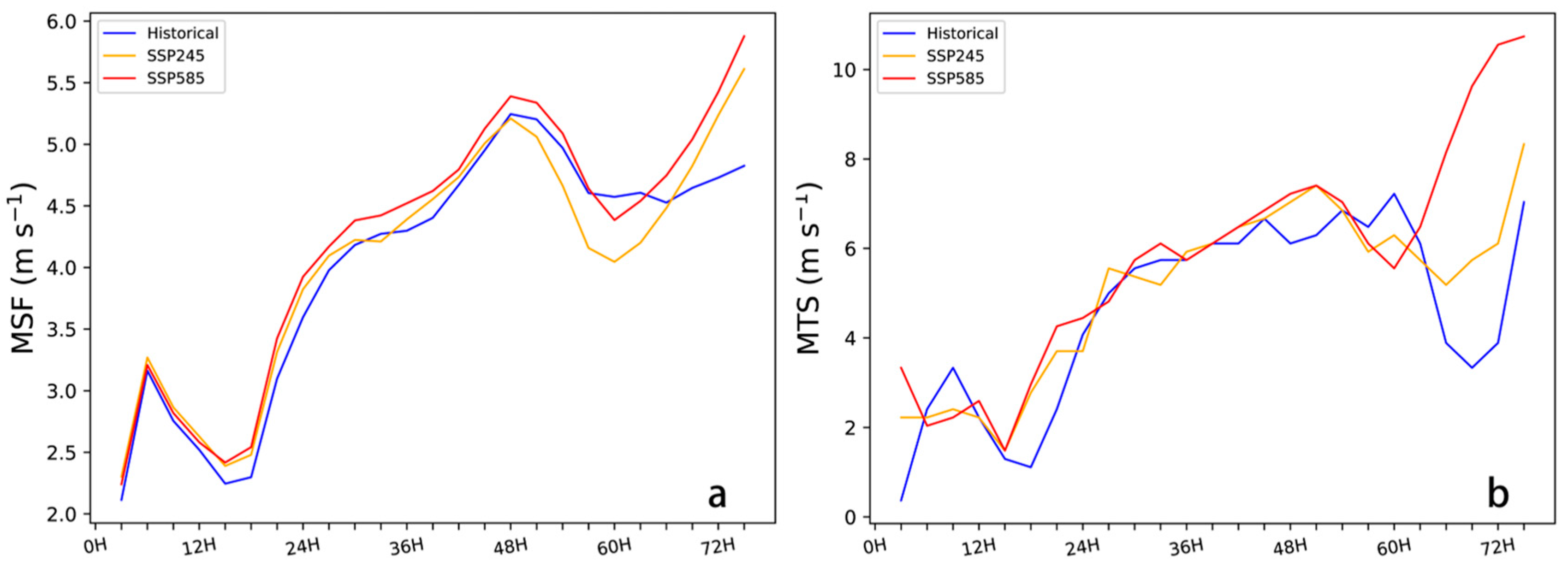
As TCs are predominantly driven by large-scale environmental flows [56], the change in meridional steering flow is assumed to induce the poleward migration of TC under global warming. To further investigate the cause of TC poleward migration, Figure 8 depicts meridional steering flow (MSF) and TC meridional translation speed (MTS) of three carbon emissions. We define MSF using the averaged meridional flow between 850 and 300 hPa and within a 5°–7° latitude band around the TC center [57]. As shown in Figure 8, in the early stage, the MSFs in three experiments are almost the same. However, after the spin-up time of 12 h, the differences in MSFs among three runs become obvious. Except for the model time from 48 h to 66 h after the model start, the MSF increases with the carbon emissions. This indicates that the differences in MSF might be a major contributor to the poleward migration of TC track under global warming. Moreover, the change in MSF is similar to MTS, but MSF is somewhat smaller than MTS. This is consistent with Chan and Gray’s finding [56] that TCs generally move at a faster rate than the steering flow.
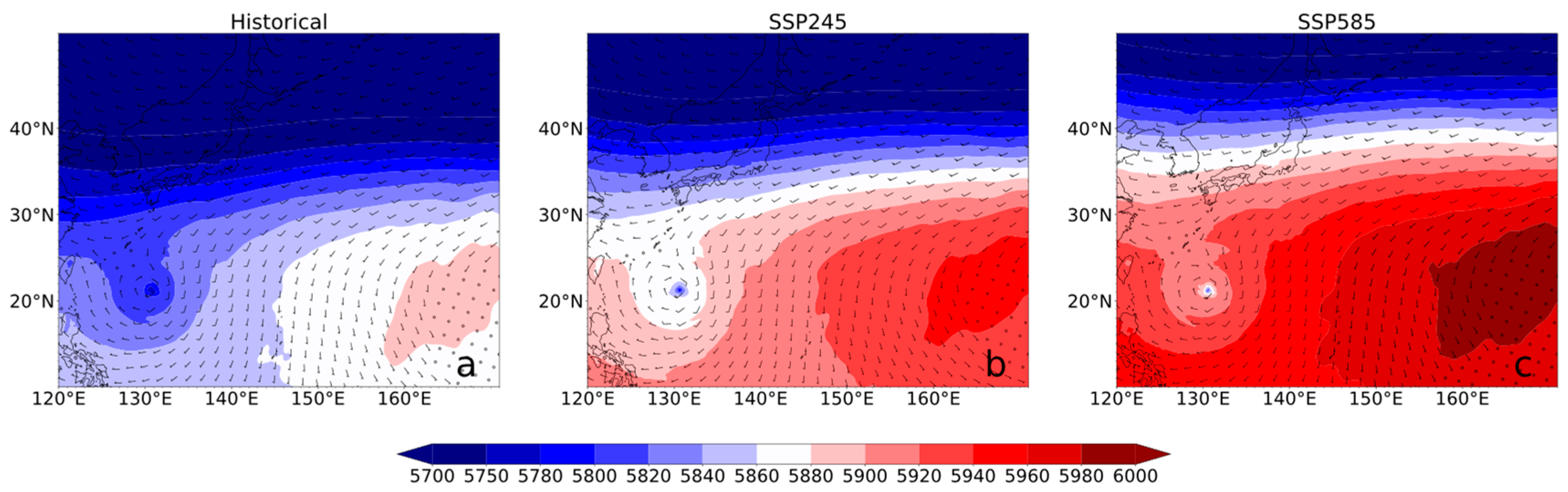
The increase in the WPSH intensity is expected under global warming if other influences of adjacent systems are not considered [58]. Earlier studies have suggested that the extending of the WPSH can affect the large-scale environmental flow, which in turn affects storm movement over the WNP [21]. To further explore the cause of the poleward steering flow and the poleward migration of TC under global warming, we designed Figure 9, which shows the simulated 500 hPa geopotential height and wind vector in three experiments. As suggested by He and Zhou [15], the 500 hPa geopotential height will increase with global warming, which makes it inaccurate to estimate the location of the WPSH by the absolute value of the 500 hPa geopotential height (e.g., 5880 m). Sun et al. [14] indicated that the first unclosed isobar line near TC, which is determined by the relative value of the 500 hPa geopotential height instead of its absolute value, can be used to evaluate the edge of the WPSH due to ocean warming. Comparison of the three carbon emissions in Figure 9 indicates that the poleward shift of TC is closely related to the WPSH expansion under global warming, namely the TC track, as well as its poleward shift, and is mainly determined by its surrounding steering flow, which is closely related to the WPSH edge near the TC. Following the increase in carbon emission, the geopotential height contours between TC and WPSH are more densely distributed, resulting in a larger pressure gradient on the right-hand side of the TC near the WPSH edge (Figure 9). This leads to a stronger meridional steering flow (Figure 8) and, thus, a farther poleward migration of the TC (Figure 7). Note that Figure 9 focuses on the situation before significant differences in simulated TC locations (e.g., 6 h after the model start), because once the location difference increases to a significant level, the TCs at different locations may affect the intensity of the simulated WPSH, which complicates the causal relationship of the poleward migration of TC with the WPSH [19].
3.4. TC Intensity
3.4.1. Sensitivity of TC Intensity to Carbon Emission Level
To quantify the change of TC intensity with global warming, we use Figure 10 to depict time variation of minimum surface level pressure (SLP) and maximum wind speed at 10 m height in three experiments. The TC intensity increases in terms of both minimum SLP and maximum wind speed. The TC lifetime maximum intensity (LMI) in SSP245 (SSP585) is about 16.4 hPa and 5.2 m s−1 (22.6 hPa and 7.3 m s−1), stronger than those in Historical. Note that the TC intensity from SSP245 to SSP585 is obviously smaller than that from Historical and SSP245.
Among various factors contributing to TC activity, SST is known as a determinant one in TC intensity change. Warmer SST, as the direct energy source of TC, favors the genesis and development of TC [3]. The SST in TC main development region (a rectangular area of 125°–170°E, 5°–25°N) of the WNP in SSP245 (SSP585) increases about 2.04 °C (3.56 °C) compared to that in Historical. According to the air–sea interaction theory on MPI, the TC strength increases 15.6 hPa or 5.36 m s−1 following 1 °C warming in SST [59]. However, the increase in TC intensity between different experiments is not as large as predicted by the theory on MPI. The increase in TC intensity for 1 °C warming between SSP245 and Historical is 8.0 hPa and 2.5 m s−1, and that between SSP585 and SSP245 is 4.1 hPa and 1.4 m s−1. Moreover, the increase in TC intensity (i.e., maximum wind speed and minimum SLP) from SSP245 to SSP585 is obviously smaller than that from Historical to SSP245. This implies that TC intensity may not increase continuously with global warming and can reach a threshold if carbon emission still increases in the future, which was suggested in Chan et al. [60].
The change of TC intensity is mainly determined by ocean environment (e.g., surface enthalpy) and atmospheric environment (e.g., large-scale environment) [61,62]. Thereby, to reveal the possible cause for the unexpected smaller increase in TC intensity under global warming, it is necessary to analyze the differences in ocean and atmospheric environments among three emission experiments.
3.4.2. Ocean Environment
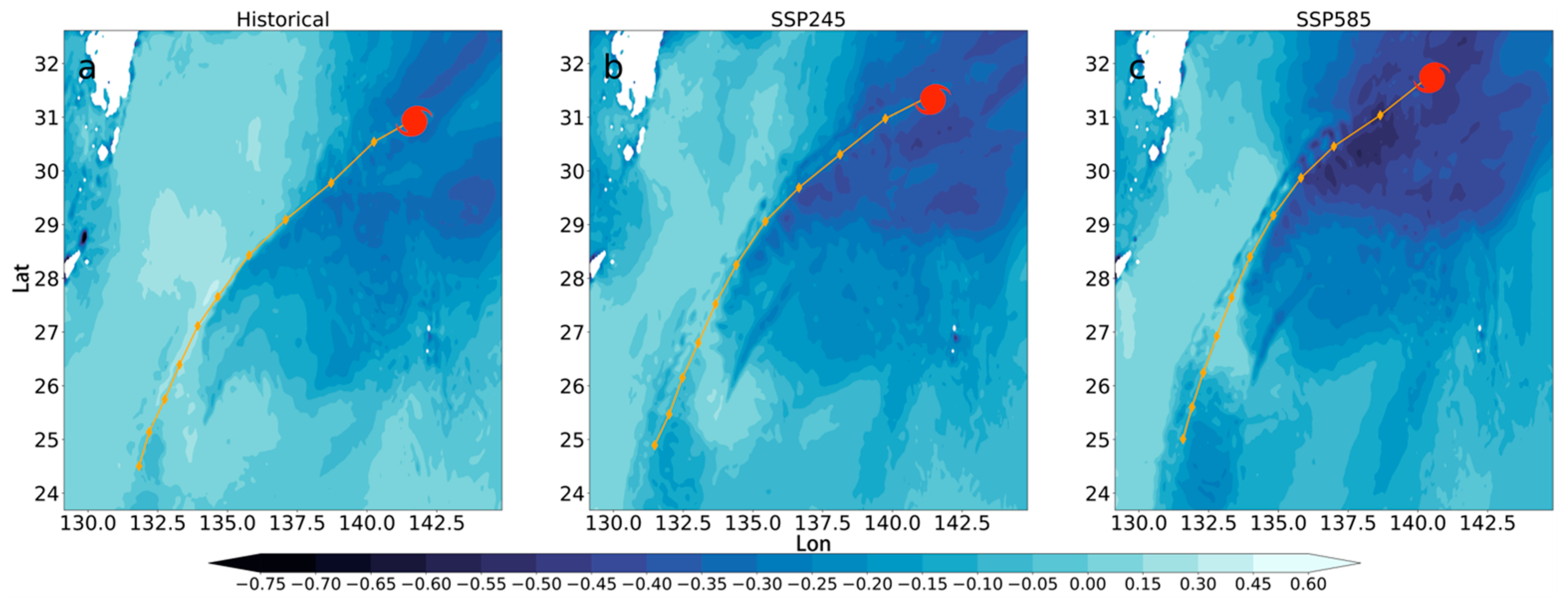
In the development of TC, ocean environment serves as one of the key determinants. The interaction between ocean environment and TC activities is not a one-way process but a bidirectional process. However, the effect from TC activities to ocean environment is not well described in the WRF model. In this study, the COAWST system has a great advantage of showing the interaction between TC and ocean environment. As is known, TC can induce significant SST cooling around the TC center. In a previous study, the TC-induced SST cooling is measured by calculating the differences between SST 1 day after the LMI moment and the initial SST [63]. To investigate the impact of global warming on TC-induced SST cooling, Figure 11 depicts the TC-induced SST cooling near the TC center in the different emission experiments. In this study, the average SST within a radius of 0–250 km around the TC center cools 0.04 °C (0.23 °C, 0.41 °C) in Historical (SSP245, SSP585) emission. It clearly shows that the influence of TC-induced SST cooling becomes obvious with the increase in carbon emission. Lloyd and Vecchi [64] suggested that the stronger TC tends to be accompanied by larger SST cooling. Thereby, following the increase in carbon emissions, it is possible that the increased TC intensity is a major driver of the increased TC-induced SST cooling, which in turn hinders the further increase in TC intensity.
Earlier studies have shown that a TC strengthens and sustains itself against surface friction loss through energy extraction from the underlying ocean [65]. Thus, the air–sea heat and energy exchange are crucial factors in the intensity change of TC [66]. SST can directly affect the energy exchange, i.e., surface enthalpy flux (SEF), which equals to the sum of sensible heat flux (SHF) and latent heat flux (LHF) and, thus, contributes greatly to TC intensity. SHF is proportional to the air–sea temperature difference (ASTD), which is defined as SST minus 2 m air temperature (T2); and LHF is proportional to the air–sea moisture difference (ASMD), which is defined as the sea-surface saturation specific humidity determined by SST minus 2 m air specific humidity (M2).
The wind-induced surface heat exchange (WISHE) is regarded as the primary process controlling the change of TC intensity, as it shows a positive feedback between the surface enthalpy flux and the surface wind speed close to a TC’s center [22,23,24]. Since SEF is directly related to SST change, we take an in-depth look at how SEF coordinates with 10 m average tangential wind speed and reacts to the change of SST in different carbon emission experiments.
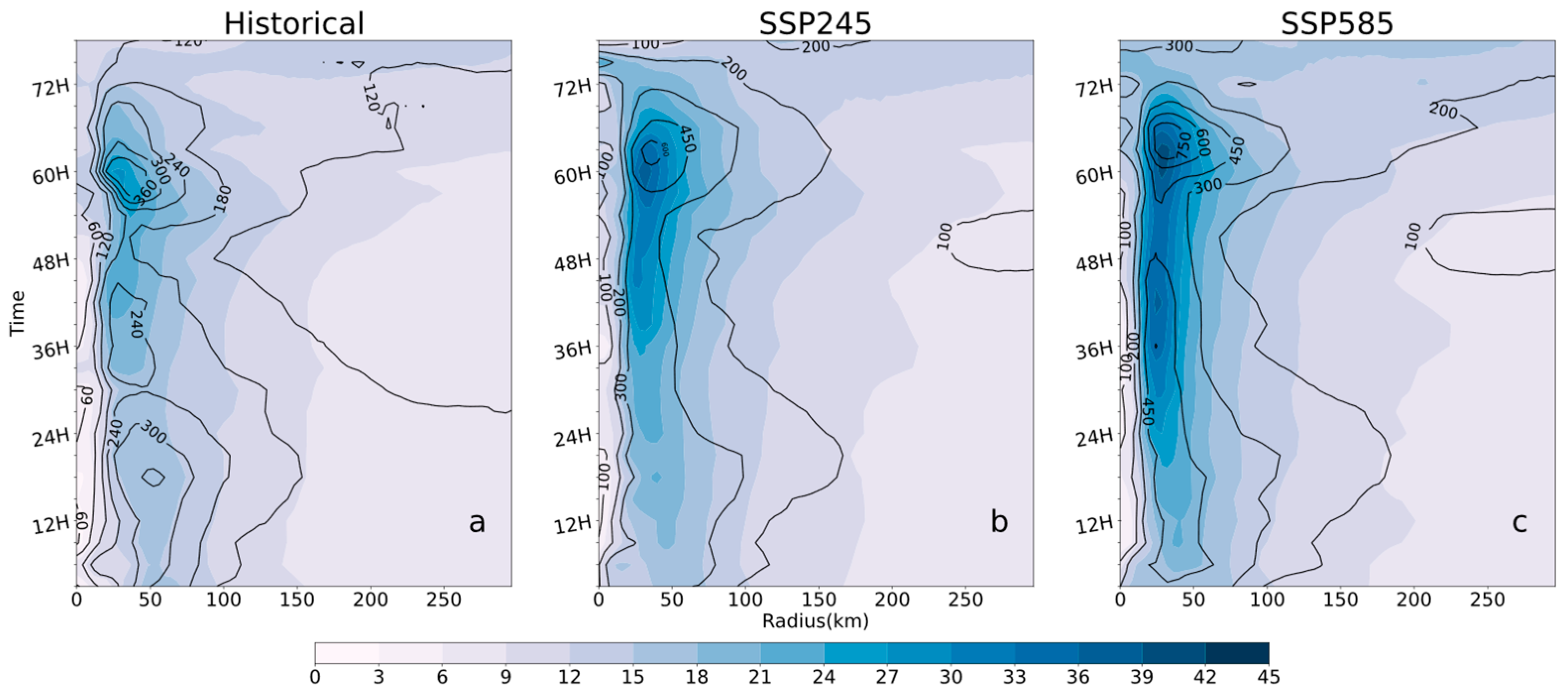
Figure 12 illustrates under three experimental conditions the radius-time cross sections of 10 m average tangential wind speed and SEF. Results clearly show that the azimuthally averaged SEF in SSP245 (SSP585) is much larger than that in Historical, both in the inner region (i.e., the region near the eyewall) and in the outer region; and SSP245 (SSP585) has a much stronger 10 m average tangential wind speed in the inner and the outer region. The larger SEF of SSP245 (SSP585) in the inner region, which is mainly concentrated in the vicinity of the eyewall, is a good helper in sustaining the TC by powering the eyewall directly and, thus, contributes largely to TC intensity [67]. Moreover, as suggested by Sun et al. [65], the larger SEF in SSP245 (SSP585) in the outer region favors the development of outer spiral rainbands and, thus, contributes to tangential wind force increase in the outer region, but this goes against the increase in tangential wind in the inner region. This may be one of the reasons for the unexpected smaller increase in TC intensity under global warming from Historical to SSP245 (SSP585).
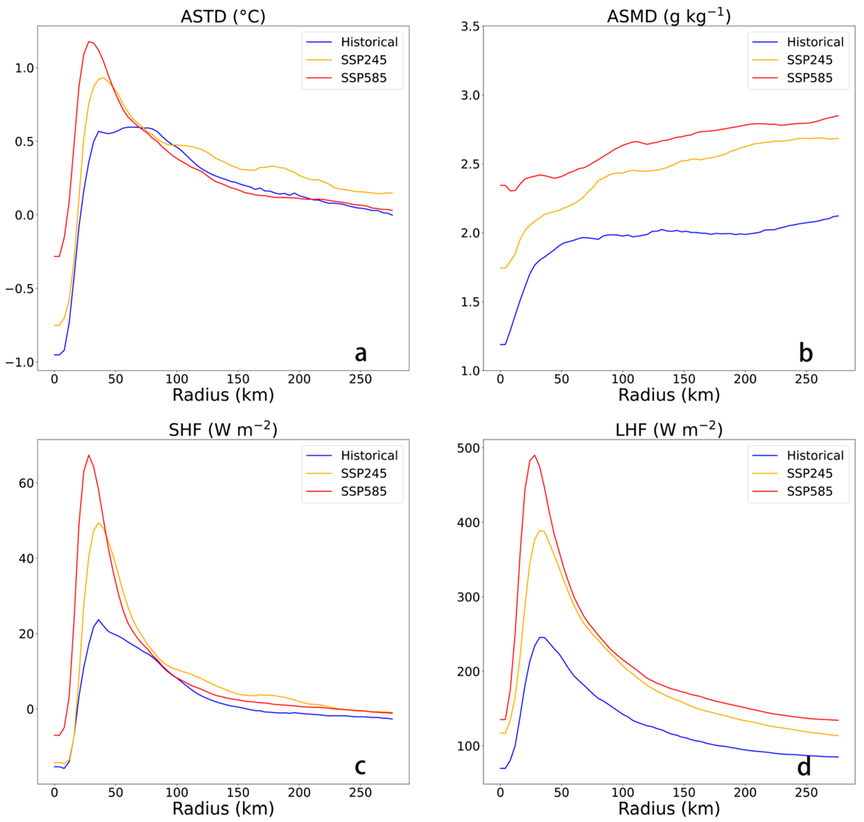
To investigate the unexpected smaller increase in TC intensity under global warming, we depict Figure 13, which shows the radial average of sea-surface enthalpy factors (i.e., ASTD, SHF, ASMD, and LHF) within a 270 km radius in three emission experiments. As mentioned in Emanuel [22], the increase in these four factors will lead flux into the eyewall and promote the convection around TC. Owing to global warming, SHF, ASTD, LHF, and ASMD near the TC center ascend in sequence of Historical, SSP245, and SSP585, which is similar with the increase trend of SST in three experiments, indicating the effect of SST on TC intensity.
The average increase in SST from Historical to SSP245 in the main development region of the WNP is 2.04 °C, and that from SSP245 to SSP585 is 1.52 °C. As for the sea-surface enthalpy factors, within the radius of 270 km, the ASTD (ASMD) increases by 0.06 °C (0.22 g kg−1) following 1 °C SST warming from Historical to SSP245 and 0.02 °C (0.16 g kg−1) from SSP245 to SSP585. As a result, the SHF (LHF), which is largely determined by ASTD (ASMD), increases by 3.3 W m−2 (34.8 W m−2) from Historical to SSP245 and 1.5 W m−2 (18.2 W m−2) from SSP245 to SSP585. This indicates that, the increase in SEF (i.e., the sum of SHF and LHF) from Historical to SSP245 (38.1 W m−2) nearly doubles the increase in SEF from SSP245 to SSP585 (19.7 W m−2). This is basically consistent with the changes of TC intensity which increase by 5.23 m s−1 from Historical to SSP245 and 2.05 m s−1 from SSP245 to SSP585. Therefore, the mentioned change of SEF, especially that of LHF, may be the main reason for the relatively smaller increase in TC intensity from SSP245 to SSP585, compared with the increase in TC intensity from Historical to SSP245.
In addition to the range and size of SST variability, the TC intensity increase is related to the mean SST itself. As discovered by Chan et al. [60], TC intensifies rapidly at an SST of 27–30 °C but slows down at an SST of above 30 °C, suggesting that 30 °C may be a critical temperature for TC intensification. The TC main development region SST of the WNP in Historical (SSP245, SSP585) is about 27.98 °C (30.02 °C, 31.54 °C). In SSP585, SST has exceeded 30 °C, which may be a reason why TC intensity cannot increase sharply from SSP245 to SSP585.
3.4.3. Atmospheric Environment
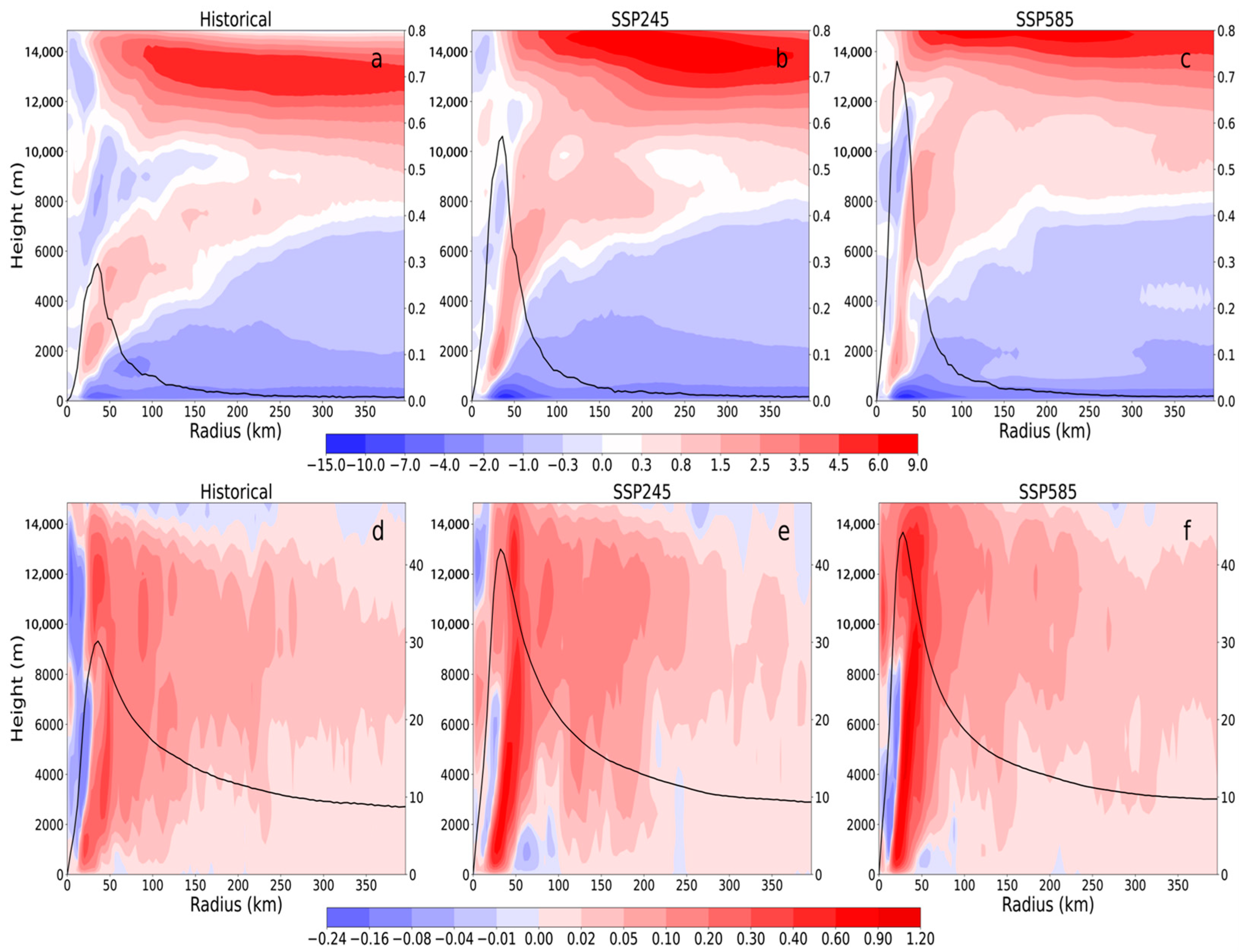
The mechanism of global warming affecting TC activity has been addressed previously. The focus has been on whether the change in SST enables the modification of the TC activities in the tropics [68,69,70]. Besides the change in ocean environment, the change in atmospheric environment also plays a determinant role in TC intensity under global warming. Figure 14 shows the time- and azimuthal-averaged distributions of TC structure including TC radial velocity, SLP gradient, vertical velocity, and surface tangential velocity in three emission experiments. As suggested by Houze et al. [71,72], the energy exchange at the air–sea interface increases, thus, the enhancement of convection around the eyewall under global warming. In this study, the TC convection (e.g., vertical velocity) near the eyewall becomes stronger in sequence of Historical, SSP245, and SSP585 (Figure 14a–c). A stronger convection is often accompanied by a stronger SLP gradient, which promotes eyewall slope [73]. The SLP gradient also ascends in sequence of Historical, SSP245, and SSP585; and the maximum SLP gradient is 0.29, 0.57, and 0.73 hPa km−1 in Historical, SSP245, and SSP585, respectively. The SLP gradient enhancement makes surface tangential velocity increase, thus producing a stronger wind speed around the TC, which increases TC intensity [74].
On the other hand, the change of eyewall slope is also a reason for the TC-intensity difference among the three experiments. The upwelling air parcel in the eyewall generally experiences a drop in the inward directed pressure gradient force, resulting in centrifugal displacement outwards with growing height—that is, the eyewall slope [75]. Stern and Nolan [76], based on observations, found that there is a certain relationship between the eyewall slope and TC intensity, which is affected by the radial pressure gradient. On top of all of that, a less upright eyewall is often linked with suppressed storm intensification, because it is usually accompanied by weaker radial gradients of tangential velocity, vertical velocity, and pressure. On the contrary, the relation of a more upright eyewall to stronger radial gradients of vertical velocity and pressure, which promotes storm intensification, was noted [73,77]. In Figure 14a–c, the changes of vertical velocity and pressure gradient associated with steep eyewall slope, which indicate a more upright TC structure, may be one of the reasons for TC intensity increase. It is important to note that the SLP gradient, as well as the eyewall slope, changes greatly (slightly) from Historical (SSP245) to SSP245 (SSP585), which contributes to the large (small) increase in TC intensity from Historical (SSP245) to SSP245 (SSP585), and thus eventually partly explains the reason for the unexpected smaller increase in TC intensity under global warming.
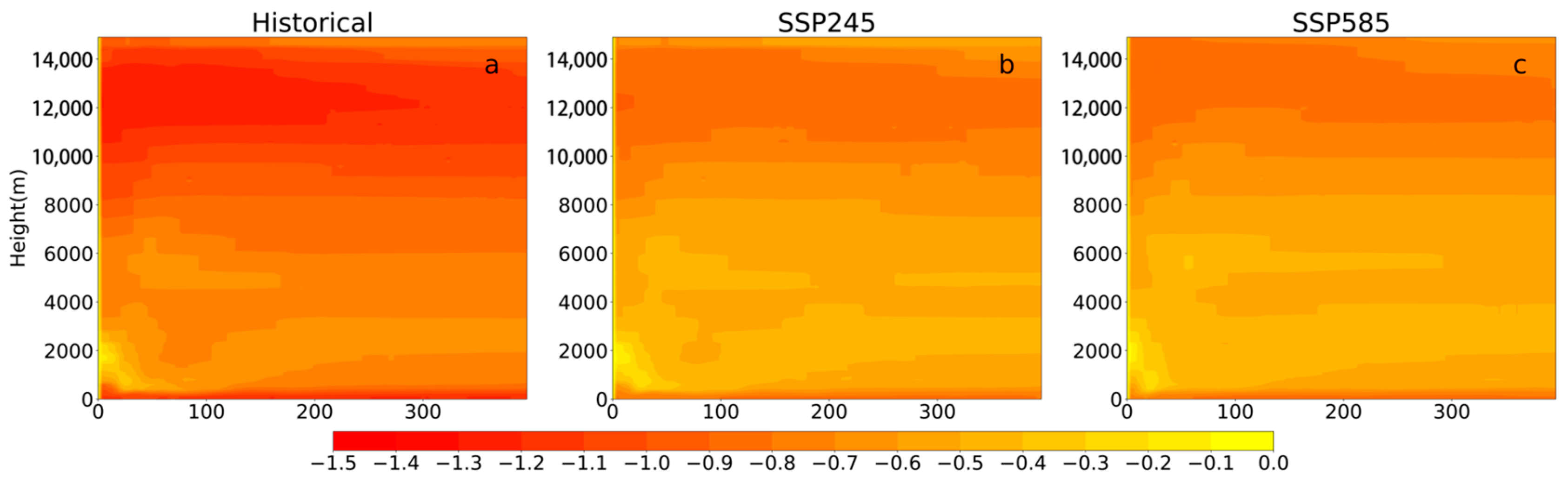
As suggested by Downs and Kieu [78], the increase in tropospheric stability has a negative effect on TC intensity, thus partially offsetting the estimated increase in TC potential intensity. Figure 15 shows time- and azimuthal-averaged instability of three emission experiments. Although the TC is weaker in Historical (Figure 10), the instability of atmospheric structure in Historical is bigger than that in SSP245 and SSP585. According to Downs and Kieu [78], the relatively more stable structure in SSP245 and SSP585 reduces the intensity of convective activity around the TC and, thus, inhibits the development of TC intensity. This may be a reason why TC intensity increases not as sharply as predicted.
In addition to the increase in SST, global warming also changes the temperature profile of the tropical troposphere. Generally, the upper tropospheric temperature rises and falls in consistency with the underlying SST in the tropics [68,69]. TC activities are affected by atmospheric circulation, especially the upper tropospheric temperature [65].
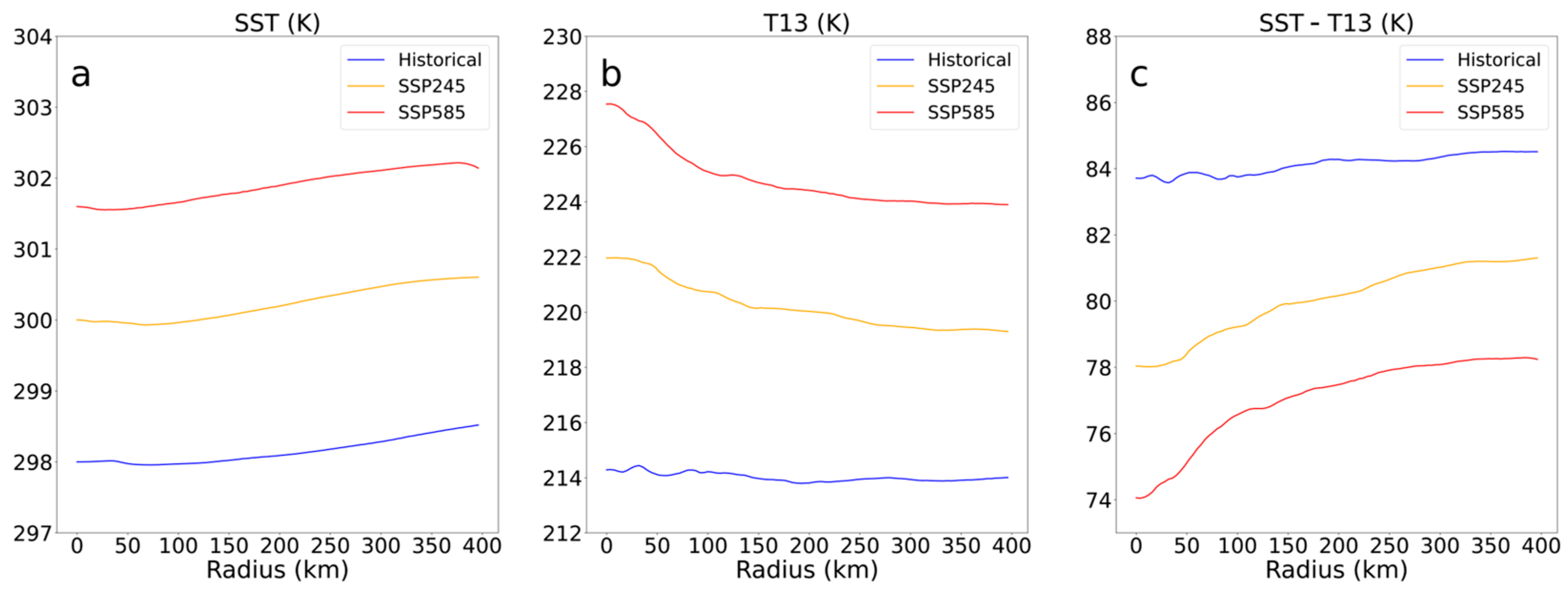
According to the Carnot cycle theory of Emanuel [22,29], the stronger difference between the temperature at the outflow height and the underlying SST near the TC is beneficial to TC development and, thus, a stronger TC maximum potential intensity. Ryglicki et al. [79] suggested that the outflow height is around 12–14 km. To further investigate the unexpected smaller increase in TC intensity, we use Figure 16 to show the difference between azimuthal-averaged temperature at a height of 13 km around TC (T13) and SST at LMI moment. With the increase in carbon emission, SST and T13 both increases, but the difference between them decreases notably as the increase in SST is smaller than the increase in T13. The decreased difference indicates a more stable atmospheric condition and, thus, disfavors the increase in TC intensity. This is an important reason for the unexpected smaller increase in TC intensity under global warming.
4. Conclusions
The effect of global warming on TC track and intensities has been a hot topic. Based on IBTrACS dataset, we investigate the variation of TC track and intensity from 1980 to 2021, which is consistent with previous studies. However, the data inhomogeneity in remote sensing and large natural variability may influence the result. To improve our understanding on the effect of global warming on TC track and intensity, the coupled modeling system (COAWST) is used to investigate possible mechanisms via a suite of sensitivity experiments. In all of our experiments, the initial TC location and intensity in the TC Bogus scheme are the same. This allows us to effectively investigate how global warming affects TC track and intensity without the interference of initial conditions.
Results of our three carbon emission experiments indicate that the simulated TC tends to migrate poleward under global warming, which is consistent with existing studies [14,16,17]. The involved mechanisms are also revealed in this study. Under global warming, the WPSH expands notably, resulting in a larger pressure gradient on the right side of TC near the WPSH edge. This further contributes to the increase in stronger poleward steering flow and eventually drives the TC to shift poleward.
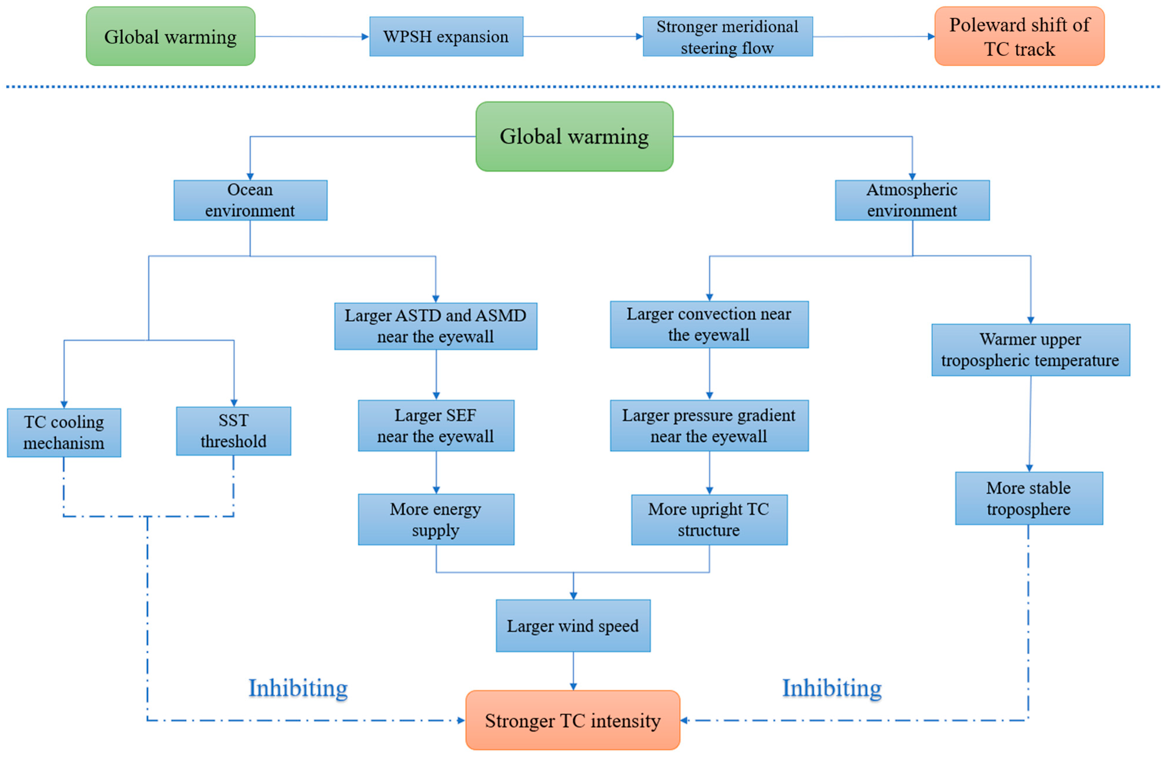
Our results also indicate that TC intensity increases with global warming. The involved mechanisms are revealed by examining ocean environment and atmospheric environment, which are schematically summarized in Figure 17. From the viewpoint of ocean environment, with the increase in carbon emissions, larger ASTD and ASMD appear near the eyewall, and thus, more SEF enters the eyewall, which supplies more energy to the TC. Meanwhile, from the viewpoint of atmospheric environment, with the increase in carbon emissions, the convection near the eyewall becomes stronger, which leads to larger pressure gradient near the eyewall and, thus, the more upright TC structure. Under joint effect of more energy supply and more upright TC structure, the wind speed and, thus, the TC intensity increase, namely TC intensity follows the sequence of Historical, SSP245, and SSP585.
Our results also indicate that the increase in TC intensity is far smaller than that predicted by MPI theory. Moreover, the relationship between the increase in TC intensity and global warming is not linear, as the increase in TC intensity from SSP245 to SSP585 is obviously smaller than that from Historical to SSP245. The reasons for the unexpected smaller increase in TC intensity are also investigated in this study. First, the TC-induced cooling plays a negative role in determining TC intensity and is more obvious when TC intensity increases with global warming. Second, the increase in TC intensity following global warming has a threshold, as the TC intensity experiences rapid intensification at an SST of 27–30 °C (e.g., from Historical to SSP245) but slows down when the SST is above 30 °C (e.g., from SSP245 to SSP585). Third, the upper tropospheric temperature increases more than SST does under global warming, resulting in more stable atmospheric condition, which goes against the TC intensification. In this study, the negative effects of the above three factors make the increase in TC intensity less than predicted by the previous theory on MPI. Furthermore, these negative effects become stronger following global warming, and thus, the increase in TC intensity from SSP245 to SSP585 is notably weaker than that from Historical to SSP245.
The response of TC intensity to global warming remains controversial; and our results are far from being sufficient to provide insight into global warming on TC track and intensity as one single TC case is vulnerable to other factors, which are outside the scope of this study. Thereby, more TC cases need to be studied in future to draw a robust conclusion on this issue.
Author Contributions
Conceptualization, Y.S. (Yuan Sun); methodology, Y.S. (Yuan Sun) and Z.F.; software, Z.F.; validation, Y.Y. and L.Z.; formal analysis, Z.F. and Y.S. (Yuan Sun); investigation, Z.F. and Y.S. (Yuan Sun); resources, Y.S. (Yuan Sun); data curation, Z.F. and Y.S. (Yixuan Shen); writing—original draft preparation, Z.F.; writing—review and editing, Y.S. (Yuan Sun) and J.S.; visualization, Z.F. and S.L.; supervision, Y.S. (Yuan Sun) and J.S.; project administration, Y.S. (Yuan Sun) and J.S.; funding acquisition, Y.S. (Yuan Sun), W.Z. and Y.Y. All authors have read and agreed to the published version of the manuscript.
Funding
This research was supported by the National Natural Science Foundation of China (Grants 42075035, 42075011 and 42005025) and the Scientific Research Fund of National University of Defense Technology (ZK20-34).
Data Availability Statement
The data are obtained by the sixth phase of the Coupled Model Intercomparison Project. The reader can calculate the corresponding data according to the parameters in the paper.
Conflicts of Interest
The authors declare no conflict of interest.
References
- Pielke, R.A., Jr.; Gratz, J.; Landsea, C.W.; Collins, D.; Saunders, M.A.; Musulin, R. Normalized hurricane damage in the United States: 1900–2005. Nat. Hazards Rev. 2008, 9, 29–42. [Google Scholar] [CrossRef]
- Peduzzi, P.; Chatenoux, B.; Dao, H.; De Bono, A.; Herold, C.; Kossin, J.; Mouton, F.; Nordbeck, O. Global trends in tropical cyclone risk. Nat. Clim. Chang. 2012, 2, 289–294. [Google Scholar] [CrossRef]
- Emanuel, K. Increasing destructiveness of tropical cyclones over the past 30 years. Nature 2005, 436, 686–688. [Google Scholar] [CrossRef] [PubMed]
- Emanuel, K.; Ravela, S.; Vivant, E.; Risi, C. A statistical deterministic approach to hurricane risk assessment. Bull. Am. Meteorol. Soc. 2006, 87, 299–314. [Google Scholar] [CrossRef]
- Dixon, A.M.; Puotinen, M.; Ramsay, H.A.; Beger, M. Coral reef exposure to damaging tropical cyclone waves in a warming climate. Earth’s Future 2022, 10, e2021EF002600. [Google Scholar] [CrossRef]
- Qin, L.; Liao, X.; Xu, W.; Meng, C.; Zhai, G. Change in Population Exposure to Future Tropical Cyclones in Northwest Pacific. Atmosphere 2023, 14, 69. [Google Scholar] [CrossRef]
- Emanuel, K.; Sundararajan, R.; Williams, J. Hurricanes and global warming: Results from downscaling IPCC AR4 simulations. Bull. Am. Meteorol. Soc. 2008, 89, 347–368. [Google Scholar] [CrossRef]
- Zhao, H.; Wu, L.; Zhou, W. Assessing the influence of the ENSO on tropical cyclone prevailing tracks in the western North Pacific. Adv. Atmos. Sci. 2010, 27, 1361–1371. [Google Scholar] [CrossRef]
- Lee, T.C.; Knutson, T.R.; Kamahori, H.; Ying, M. Impacts of climate change on tropical cyclones in the western North Pacific basin. Part I: Past observations. Trop. Cyclone Res. Rev. 2012, 1, 213–235. [Google Scholar]
- Ying, M.; Knutson, T.R.; Kamahori, H.; Lee, T.C. Impacts of climate change on tropical cyclones in the western North Pacific basin. Part II: Late twenty-first century projections. Trop. Cyclone Res. Rev. 2012, 1, 231–241. [Google Scholar]
- Patricola, C.M.; Cassidy, D.J.; Klotzbach, P.J. Tropical Oceanic Influences on Observed Global Tropical Cyclone Frequency. Geophys. Res. Lett. 2022, 49, e2022GL099354. [Google Scholar] [CrossRef]
- Gori, A.; Lin, N.; Schenkel, B.; Chavas, D. North Atlantic tropical cyclone size and storm surge reconstructions from 1950-present. J. Geophys. Res. Atmos. 2023, 128, e2022JD037312. [Google Scholar] [CrossRef]
- Knutson, T.R.; McBride, J.L.; Chan, J.; Emanuel, K.; Holland, G.; Landsea, C.; Held, I.; Kossin, J.P.; Srivastava, A.K.; Sugi, M. Tropical cyclones and climate change. Nat. Geosci. 2010, 3, 157–163. [Google Scholar] [CrossRef]
- Sun, Y.; Zhong, Z.; Li, T.; Yi, L.; Camargo, S.J.; Hu, Y.; Liu, K.; Chen, H.; Liao, Q.; Shi, J. Impact of ocean warming on tropical cyclone track over the western north pacific: A numerical investigation based on two case studies. J. Geophys. Res. Atmos. 2017, 122, 8617–8630. [Google Scholar] [CrossRef]
- He, C.; Zhou, W. Different Enhancement of the East Asian summer monsoon under global warming and interglacial epochs simulated by CMIP6 models: Role of the subtropical high. J. Clim. 2020, 33, 9721–9733. [Google Scholar] [CrossRef]
- Kossin, J.P.; Emanuel, K.A.; Vecchi, G.A. The poleward migration of the location of tropical cyclone maximum intensity. Nature 2014, 509, 349–352. [Google Scholar] [CrossRef]
- Kossin, J.P.; Emanuel, K.A.; Camargo, S.J. Past and projected changes in western North Pacific tropical cyclone exposure. J. Clim. 2016, 29, 5725–5739. [Google Scholar] [CrossRef]
- Wu, L.; Chou, C.; Chen, C.-T.; Huang, R.; Knutson, T.R.; Sirutis, J.J.; Garner, S.T.; Kerr, C.; Lee, C.-J.; Feng, Y.C. Simulations of the present and late-twenty-first-century western North Pacific tropical cyclone activity using a regional model. J. Clim. 2014, 27, 3405–3424. [Google Scholar] [CrossRef]
- Zhong, Z. A possible cause of a regional climate model’s failure in simulating the east Asian summer monsoon. Geophys. Res. Lett. 2006, 33. [Google Scholar] [CrossRef]
- Sun, Y.; Zhong, Z.; Lu, W.; Hu, Y. Why are tropical cyclone tracks over the western North Pacific sensitive to the cumulus parameterization scheme in regional climate modeling? A case study for Megi (2010). Mon. Weather Rev. 2014, 142, 1240–1249. [Google Scholar] [CrossRef]
- Sun, Y.; Zhong, Z.; Yi, L.; Li, T.; Chen, M.; Wan, H.; Wang, Y.; Zhong, K. Dependence of the relationship between the tropical cyclone track and western Pacific subtropical high intensity on initial storm size: A numerical investigation. J. Geophys. Res. Atmos. 2015, 120, 11–451. [Google Scholar] [CrossRef]
- Emanuel, K.A. An air-sea interaction theory for tropical cyclones. Part I: Steady-state maintenance. J. Atmos. Sci. 1986, 43, 585–605. [Google Scholar] [CrossRef]
- Rotunno, R.; Emanuel, K.A. An air–sea interaction theory for tropical cyclones. Part II: Evolutionary study using a nonhydrostatic axisymmetric numerical model. J. Atmos. Sci. 1987, 44, 542–561. [Google Scholar] [CrossRef]
- Holland, G.J. The maximum potential intensity of tropical cyclones. J. Atmos. Sci. 1997, 54, 2519–2541. [Google Scholar] [CrossRef]
- Persing, J.; Montgomery, M.T. Is environmental CAPE important in the determination of maximum possible hurricane intensity? J. Atmos. Sci. 2005, 62, 542–550. [Google Scholar] [CrossRef]
- Bell, M.M.; Montgomery, M.T. Observed structure, evolution, and potential intensity of category 5 Hurricane Isabel (2003) from 12 to 14 September. Monthly Weather Review 2008, 136, 2023–2046. [Google Scholar] [CrossRef]
- Zhang, X.; Xu, F.; Zhang, J.; Lin, Y. Decrease of Annually Accumulated Tropical Cyclone-Induced Sea Surface Cooling and Diapycnal Mixing in Recent Decades. Geophys. Res. Lett. 2022, 49, e2022GL099290. [Google Scholar] [CrossRef]
- Tiwari, G.; Rameshan, A.; Kumar, P.; Javed, A.; Mishra, A.K. Understanding the post-monsoon tropical cyclone variability and trend over the Bay of Bengal during the satellite era. Q. J. R. Meteorol. Soc. 2022, 148, 1–14. [Google Scholar] [CrossRef]
- Emanuel, K. Tropical cyclones. Annu. Rev. Earth Planet. Sci. 2003, 31, 75–104. [Google Scholar] [CrossRef]
- Vidale, P.L.; Hodges, K.; Vannière, B.; Davini, P.; Roberts, M.J.; Strommen, K.; Weisheimer, A.; Plesca, E.; Corti, S. Impact of stochastic physics and model resolution on the simulation of tropical cyclones in climate GCMs. J. Clim. 2021, 34, 4315–4341. [Google Scholar] [CrossRef]
- Warner, J.C.; Armstrong, B.; He, R.; Zambon, J.B. Development of a coupled ocean–atmosphere–wave–sediment transport (COAWST) modeling system. Ocean Model. 2010, 35, 230–244. [Google Scholar] [CrossRef]
- Jacob, R.; Larson, J.; Ong, E. M × N communication and parallel interpolation in Community Climate System Model Version 3 using the model coupling toolkit. Int. J. High Perform. Comput. Appl. 2005, 19, 293–307. [Google Scholar] [CrossRef]
- Larson, J.; Jacob, R.; Ong, E. The model coupling toolkit: A new Fortran90 toolkit for building multiphysics parallel coupled models. Int. J. High Perform. Comput. Appl. 2005, 19, 277–292. [Google Scholar] [CrossRef]
- Warner, J.C.; Sherwood, C.R.; Signell, R.P.; Harris, C.K.; Arango, H.G. Development of a three-dimensional, regional, coupled wave, current, and sediment-transport model. Comput. Geosci. 2008, 34, 1284–1306. [Google Scholar] [CrossRef]
- Jones, P.W. A User’s Guide for SCRIP: A Spherical Coordinate Remapping and Interpolation Package; Los Alamos National Laboratory: Los Alamos, NM, USA, 1998. [Google Scholar]
- Skamarock, W.C.; Klemp, J.B.; Dudhia, J.; Gill, D.O.; Liu, Z.; Berner, J.; Wang, W.; Powers, J.G.; Duda, M.G.; Barker, D.M.; et al. A Description of the Advanced Research WRF Version 3; National Center for Atmospheric Research: Boulder, CO, USA, 2008; Note NCAR/TN-475+STR; p. 113. [Google Scholar]
- Hong, S.Y.; Lim JO, J. The WRF single-moment 6-class microphysics scheme (WSM6). Asia-Pac. J. Atmos. Sci. 2006, 42, 129–151. [Google Scholar]
- Tiedtke, M.I.C.H.A.E.L. A comprehensive mass flux scheme for cumulus parameterization in large-scale models. Mon. Weather Rev. 1989, 117, 1779–1800. [Google Scholar] [CrossRef]
- Iacono, M.J.; Delamere, J.S.; Mlawer, E.J.; Shephard, M.W.; Clough, S.A.; Collins, W.D. Radiative forcing by long-lived greenhouse gases: Calculations with the AER radiative transfer models. J. Geophys. Res. Atmos. 2008, 113. [Google Scholar] [CrossRef]
- Hong, S.Y.; Noh, Y.; Dudhia, J. A new vertical diffusion package with an explicit treatment of entrainment processes. Mon. Weather Rev. 2006, 134, 2318–2341. [Google Scholar] [CrossRef]
- Ek, M.B.; Mitchell, K.E.; Lin, Y.; Rogers, E.; Grunmann, P. Implementation of Noah land surface model advances in the National Centers for Environmental Prediction operational mesoscale Eta model. J. Geophys. Res. 2003, 108, GCP12-1. [Google Scholar] [CrossRef]
- Chassignet, E.P.; Arango, H.; Dietrich, D.; Ezer, T.; Ghil, M.; Haidvogel, D.B.; Ma, C.C.; Sirkes, Z. DAMEE-NAB: The base experiments. Dyn. Atmos. Ocean. 2000, 32, 155–183. [Google Scholar] [CrossRef]
- Haidvogel, D.B.; Arango, H.G.; Hedstrom, K.; Beckmann, A.; Malanotte-Rizzoli, P.; Shchepetkin, A.F. Model evaluation experiments in the North Atlantic Basin: Simulations in nonlinear terrain-following coordinates. Dyn. Atmos. Ocean. 2000, 32, 239–281. [Google Scholar] [CrossRef]
- Egbert, G.D.; Bennett, A.F.; Foreman, M.G. TOPEX/POSEIDON tides estimated using a global inverse model. J. Geophys. Res. Ocean. 1994, 99, 24821–24852. [Google Scholar] [CrossRef]
- Egbert, G.D.; Erofeeva, S.Y. Efficient inverse modeling of barotropic ocean tides. J. Atmos. Ocean. Technol. 2002, 19, 183–204. [Google Scholar] [CrossRef]
- Booij, N.R.R.C.; Ris, R.C.; Holthuijsen, L.H. A third-generation wave model for coastal regions: 1. Model description and validation. J. Geophys. Res. Ocean. 1999, 104, 7649–7666. [Google Scholar] [CrossRef]
- Madsen, O.S.; Poon, Y.K.; Graber, H.C. Spectral wave attenuation by bottom friction: Theory. In Coastal Engineering; ASCE: Reston, VA, USA, 1989; pp. 492–504. [Google Scholar]
- Komen, G.J.; Hasselmann, S.; Hasselmann, K. On the existence of a fully developed wind-sea spectrum. J. Phys. Oceanogr. 1984, 14, 1271–1285. [Google Scholar] [CrossRef]
- Low-Nam, S.; Davis, C. Development of a tropical cyclone bogussing scheme for the MM5 system. In Preprints, 11th PSU–NCAR Mesoscale Model Users’ Workshop, Boulder, CO, PSU–NCAR; National Center for Atmospheric Research: Boulder, CO, USA, 2001; Volume 130, p. 134. [Google Scholar]
- Hendricks, E.A.; Peng, M.S.; Ge, X.; Li, T. Performance of a dynamic initialization scheme in the Coupled Ocean–Atmosphere Mesoscale Prediction System for tropical cyclones (COAMPS-TC). Weather Forecast. 2001, 26, 650–663. [Google Scholar] [CrossRef]
- Rappin, E.D.; Nolan, D.S.; Majumdar, S.J. A highly configurable vortex initialization method for tropical cyclones. Mon. Weather Rev. 2013, 141, 3556–3575. [Google Scholar] [CrossRef]
- Camargo, S.J.; Robertson, A.W.; Gaffney, S.J.; Smyth, P.; Ghil, M. Cluster analysis of typhoon tracks. Part II: Large-scale circulation and ENSO. J. Clim. 2007, 20, 3654–3676. [Google Scholar] [CrossRef]
- Liu, K.S.; Chan, J.C.L. Interdecadal variability of western North Pacific tropical cyclone tracks. J. Clim. 2008, 21, 4464–4476. [Google Scholar] [CrossRef]
- Mei, W.; Xie, S.-P.; Zhao, M.; Wang, Y. Forced and internal variability of tropical cyclone track density in the western North Pacific. J. Clim. 2015, 28, 143–167. [Google Scholar] [CrossRef]
- Chan, D.; Wu, Q. Attributing observed SST trends and subcontinental land warming to anthropogenic forcing during 1979–2005. J. Clim. 2015, 28, 3152–3170. [Google Scholar] [CrossRef]
- Chan, J.C.; Gray, W.M. Tropical cyclone movement and surrounding flow relationships. Mon. Weather Rev. 1982, 110, 1354–1374. [Google Scholar] [CrossRef]
- Holland, G.J. Tropical cyclone motion. In Global Guide to Tropical Cyclone Forecasting; World Meteorological Organization Tech.: Geneva, Switzerland, 1993; Document WMO/TD; p. 560. [Google Scholar]
- Pan, Y.H.; Oort, A.H. Global climate variations connected with sea surface temperature anomalies in the eastern equatorial Pacific Ocean for the 1958–73 period. Mon. Weather Rev. 1983, 111, 1244–1258. [Google Scholar] [CrossRef]
- Hobgood, J.S. Maximum potential intensities of tropical cyclones near Isla Socorro, Mexico. Weather Forecast. 2003, 18, 1129–1139. [Google Scholar] [CrossRef]
- Chan, J.C.; Duan, Y.; Shay, L.K. Tropical cyclone intensity change from a simple ocean–atmosphere coupled model. J. Atmos. Sci. 2001, 58, 154–172. [Google Scholar] [CrossRef]
- Emanuel, K.; DesAutels, C.; Holloway, C.; Korty, R. Environmental control of tropical cyclone intensity. J. Atmos. Sci. 2004, 61, 843–858. [Google Scholar] [CrossRef]
- Wang, Y.Q.; Wu, C.C. Current understanding of tropical cyclone structure and intensity changes—A review. Meteorol. Atmos. Phys. 2004, 87, 257–278. [Google Scholar] [CrossRef]
- Lee, C.Y.; Chen, S.S. Stable boundary layer and its impact on tropical cyclone structure in a coupled atmosphere–ocean model. Mon. Weather Rev. 2014, 142, 1927–1944. [Google Scholar] [CrossRef]
- Lloyd, I.D.; Vecchi, G.A. Observational evidence for oceanic controls on hurricane intensity. J. Clim. 2011, 24, 1138–1153. [Google Scholar] [CrossRef]
- Sun, Y.; Zhong, Z.; Yi, L.; Ha, Y.; Sun, Y. The opposite effects of inner and outer sea surface temperature on tropical cyclone intensity. J. Geophys. Res. Atmos. 2014, 119, 2193–2208. [Google Scholar] [CrossRef]
- Malkus, J.S.; Riehl, H. On the dynamics and energy transformations in steady-state hurricanes. Tellus 1960, 12, 1–20. [Google Scholar] [CrossRef]
- Xu, J.; Wang, Y. Sensitivity of tropical cyclone inner-core size and intensity to the radial distribution of surface entropy flux. J. Atmos. Sci. 2010, 67, 1831–1852. [Google Scholar] [CrossRef]
- Vecchi, G.A.; Soden, B.J. Effect of remote sea surface temperature change on tropical cyclone potential intensity. Nature 2007, 450, 1066–1070. [Google Scholar] [CrossRef] [PubMed]
- Vecchi, G.A.; Swanson, K.L.; Soden, B.J. Whither hurricane activity? Science 2008, 322, 687–689. [Google Scholar] [CrossRef]
- Ramsay, H.A.; Sobel, A.H. Effects of relative and absolute sea surface temperature on tropical cyclone potential intensity using a single-column model. J. Clim. 2011, 24, 183–193. [Google Scholar] [CrossRef]
- Houze, R.A., Jr.; Chen, S.S.; Lee, W.C.; Rogers, R.F.; Moore, J.A.; Stossmeister, G.J.; Bell, M.M.; Cetrone, J.; Zhao, W.; Brodzik, S.R. The hurricane rainband and intensity change experiment: Observations and modeling of Hurricanes Katrina, Ophelia, and Rita. Bull. Am. Meteorol. Soc. 2006, 87, 1503–1522. [Google Scholar] [CrossRef]
- Houze, R.A., Jr.; Chen, S.S.; Smull, B.F.; Lee, W.C.; Bell, M.M. Hurricane intensity and eyewall replacement. Science 2007, 315, 1235–1239. [Google Scholar] [CrossRef]
- Fierro, A.O.; Rogers, R.F.; Marks, F.D.; Nolan, D.S. The impact of horizontal grid spacing on the microphysical and kinematic structures of strong tropical cyclones simulated with the WRF-ARW model. Mon. Weather Rev. 2009, 137, 3717–3743. [Google Scholar] [CrossRef]
- Shimada, U.; Sawada, M.; Yamada, H. Evaluation of the accuracy and utility of tropical cyclone intensity estimation using single ground-based Doppler radar observations. Mon. Weather Rev. 2016, 144, 1823–1840. [Google Scholar] [CrossRef]
- Gentry, M.S.; Lackmann, G.M. Sensitivity of simulated tropical cyclone structure and intensity to horizontal resolution. Mon. Weather Rev. 2010, 138, 688–704. [Google Scholar] [CrossRef]
- Stern, D.P.; Nolan, D.S. Reexamining the vertical structure of tangential winds in tropical cyclones: Observations and theory. J. Atmos. Sci. 2009, 66, 3579–3600. [Google Scholar] [CrossRef]
- Sun, Y.; Yi, L.; Zhong, Z.; Hu, Y.; Ha, Y. Dependence of model convergence on horizontal resolution and convective parameterization in simulations of a tropical cyclone at gray-zone resolutions. J. Geophys. Res. Atmos. 2013, 118, 7715–7732. [Google Scholar] [CrossRef]
- Downs, A.; Kieu, C. A look at the relationship between the large-scale tropospheric static stability and the tropical cyclone maximum intensity. J. Clim. 2020, 33, 959–975. [Google Scholar] [CrossRef]
- Ryglicki, D.R.; Doyle, J.D.; Hodyss, D.; Cossuth, J.H.; Jin, Y.; Viner, K.C.; Schmidt, J.M. The unexpected rapid intensification of tropical cyclones in moderate vertical wind shear. Part III: Outflow–environment interaction. Mon. Weather Rev. 2019, 147, 2919–2940. [Google Scholar] [CrossRef]
Figure 1.
Domains of WRF (D01 and D02, two-way nested), ROMS, and SWAN models (ROMS and SWAN models have the same grids).
Figure 1.
Domains of WRF (D01 and D02, two-way nested), ROMS, and SWAN models (ROMS and SWAN models have the same grids).

Figure 2.
Configurations of COAWST involving the WRF, ROMS, and SWAN models and exchanged data fields.
Figure 2.
Configurations of COAWST involving the WRF, ROMS, and SWAN models and exchanged data fields.

Figure 3.
Time evolutions of TC latitude with maximum intensity from 1980 to 2021. (a) IBTrACS; (b) JTWC; (c) JMA; (d) CMA; (e) HKO; (f) average of JTWC, JMA, CMA, and HKO.
Figure 3.
Time evolutions of TC latitude with maximum intensity from 1980 to 2021. (a) IBTrACS; (b) JTWC; (c) JMA; (d) CMA; (e) HKO; (f) average of JTWC, JMA, CMA, and HKO.

Figure 4.
Time evolutions of maximum TC intensity from 1980 to 2021. (a) IBTrACS; (b) JTWC; (c) JMA; (d) CMA; (e) HKO; (f) average of JTWC, JMA, CMA, and HKO.
Figure 4.
Time evolutions of maximum TC intensity from 1980 to 2021. (a) IBTrACS; (b) JTWC; (c) JMA; (d) CMA; (e) HKO; (f) average of JTWC, JMA, CMA, and HKO.

Figure 5.
Residual of TC latitude and TC intensity from 1980 to 2021 excluding large natural variability. (a,e) ENSO; (b,f) PDO; (c,g) IPO; (d,h) all three.
Figure 5.
Residual of TC latitude and TC intensity from 1980 to 2021 excluding large natural variability. (a,e) ENSO; (b,f) PDO; (c,g) IPO; (d,h) all three.

Figure 6.
Spatial distributions of Climatological mean SST (°C) in the three experiments: (a) Historical, (b) SSP245, (c) SSP585, (d) SSP245 minus Historical, (e) SSP585 minus Historical, and (f) SSP585 minus SSP245.
Figure 6.
Spatial distributions of Climatological mean SST (°C) in the three experiments: (a) Historical, (b) SSP245, (c) SSP585, (d) SSP245 minus Historical, (e) SSP585 minus Historical, and (f) SSP585 minus SSP245.

Figure 7.
The simulated TC track at 3 h interval in the three experiments with various carbon emissions.
Figure 7.
The simulated TC track at 3 h interval in the three experiments with various carbon emissions.

Figure 8.
Time evolutions of (a) TC meridional steering flow (m s−1) and (b) TC meridional translation speed (m s−1) in three carbon emission experiments.
Figure 8.
Time evolutions of (a) TC meridional steering flow (m s−1) and (b) TC meridional translation speed (m s−1) in three carbon emission experiments.

Figure 9.
Geopotential height at 500 hPa (m) and wind vector of the three carbon emissions at the 6 h after the model start in (a) Historical, (b) SSP245, and (c) SSP585.
Figure 9.
Geopotential height at 500 hPa (m) and wind vector of the three carbon emissions at the 6 h after the model start in (a) Historical, (b) SSP245, and (c) SSP585.

Figure 10.
Temporal evolutions of TC intensity in three carbon emission experiments. (a) minimum SLP and (b) maximum wind speed at 10 m height.
Figure 10.
Temporal evolutions of TC intensity in three carbon emission experiments. (a) minimum SLP and (b) maximum wind speed at 10 m height.

Figure 11.
Differences between SST 1 day after the LMI moment and the initial SST, which are also overlapped by the simulated TC tracks in (a) Historical, (b) SSP245, and (c) SSP585. Orange dots and lines denote the TC center and its track at 3 h interval, and red dot denote the TC center at the LMI moment.

Figure 12.
Radius-time cross section of 10 m average tangential wind speed (m s−1; shading) and SEF (W m−2; contour) in (a) Historical, (b) SSP245, and (c) SSP585.
Figure 12.
Radius-time cross section of 10 m average tangential wind speed (m s−1; shading) and SEF (W m−2; contour) in (a) Historical, (b) SSP245, and (c) SSP585.

Figure 13.
Time- and azimuthal-averaged sea-surface enthalpy of the three emission experiments during their mature stages. (a) ASTD, (b) ASMD, (c) SHF, (d) LHF. All calculations are performed over the mature stage when the difference between TC maximum wind speed and LMI is within 10 m s−1.
Figure 13.
Time- and azimuthal-averaged sea-surface enthalpy of the three emission experiments during their mature stages. (a) ASTD, (b) ASMD, (c) SHF, (d) LHF. All calculations are performed over the mature stage when the difference between TC maximum wind speed and LMI is within 10 m s−1.

Figure 14.
Time- and azimuthal-averaged TC structure for the three emission experiments. (a–c) Radial velocity (shading; m s−1) and SLP gradient (contour; hPa km−1); (d–f) vertical velocity (shading; m s−1) and surface tangential velocity (contour; m s−1). All calculations are performed over the mature stage.

Figure 15.
Time- and azimuthal-averaged instability (°C/100 m) in (a) Historical, (b) SSP245, and (c) SSP585. All calculations are performed over their mature stages.
Figure 15.
Time- and azimuthal-averaged instability (°C/100 m) in (a) Historical, (b) SSP245, and (c) SSP585. All calculations are performed over their mature stages.

Figure 16.
Azimuthal-averaged temperature at LMI moment of the three emission experiments: (a) SST, (b) T13, and (c) difference between SST and T13.
Figure 16.
Azimuthal-averaged temperature at LMI moment of the three emission experiments: (a) SST, (b) T13, and (c) difference between SST and T13.

Figure 17.
Schematic diagram of possible mechanisms explaining the impact of global warming on TC track and intensity. Solid arrow means positive effect, and dotted arrow means negative effect.
Figure 17.
Schematic diagram of possible mechanisms explaining the impact of global warming on TC track and intensity. Solid arrow means positive effect, and dotted arrow means negative effect.

Disclaimer/Publisher’s Note: The statements, opinions and data contained in all publications are solely those of the individual author(s) and contributor(s) and not of MDPI and/or the editor(s). MDPI and/or the editor(s) disclaim responsibility for any injury to people or property resulting from any ideas, methods, instructions or products referred to in the content. |
© 2023 by the authors. Licensee MDPI, Basel, Switzerland. This article is an open access article distributed under the terms and conditions of the Creative Commons Attribution (CC BY) license (https://creativecommons.org/licenses/by/4.0/).
Share and Cite
MDPI and ACS Style
Feng, Z.; Shi, J.; Sun, Y.; Zhong, W.; Shen, Y.; Lv, S.; Yao, Y.; Zhao, L. Impact of Global Warming on Tropical Cyclone Track and Intensity: A Numerical Investigation. Remote Sens. 2023, 15, 2763. https://doi.org/10.3390/rs15112763
AMA Style
Feng Z, Shi J, Sun Y, Zhong W, Shen Y, Lv S, Yao Y, Zhao L. Impact of Global Warming on Tropical Cyclone Track and Intensity: A Numerical Investigation. Remote Sensing. 2023; 15(11):2763. https://doi.org/10.3390/rs15112763
Chicago/Turabian StyleFeng, Zhihao, Jian Shi, Yuan Sun, Wei Zhong, Yixuan Shen, Shuo Lv, Yao Yao, and Liang Zhao. 2023. "Impact of Global Warming on Tropical Cyclone Track and Intensity: A Numerical Investigation" Remote Sensing 15, no. 11: 2763. https://doi.org/10.3390/rs15112763
Note that from the first issue of 2016, this journal uses article numbers instead of page numbers. See further details here.