

Self-Supervised Remote Sensing Image Dehazing Network Based on Zero-Shot Learning

1
College of Photonic and Electronic Engineering, Fujian Normal University, Fuzhou 350117, China
2
College of Electronics and Information Science, Fujian Jiangxia University, Fuzhou 350108, China
3
The Smart Home Information Collection and Processing on Internet of Things Laboratory of Digital Fujian, Fuzhou 350108, China
4
College of Finance, Fujian Jiangxia University, Fuzhou 350108, China
*
Author to whom correspondence should be addressed.
Remote Sens. 2023, 15(11), 2732; https://doi.org/10.3390/rs15112732
Submission received: 11 April 2023
/
Revised: 19 May 2023
/
Accepted: 22 May 2023
/
Published: 24 May 2023
(This article belongs to the Special Issue Convolutional Neural Network Applications in Remote Sensing II)
Abstract
:Traditional dehazing approaches that rely on prior knowledge exhibit limited efficacy when confronted with the intricacies of real-world hazy environments. While learning-based dehazing techniques necessitate large-scale datasets for effective model training, the acquisition of these datasets is time-consuming and laborious, and the resulting models may encounter a domain shift when processing real-world hazy images. To overcome the limitations of prior-based and learning-based dehazing methods, we propose a self-supervised remote sensing (RS) image-dehazing network based on zero-shot learning, where the self-supervised process avoids dense dataset requirements and the learning-based structures refine the artifacts in extracted image priors caused by complex real-world environments. The proposed method has three stages. The first stage involves pre-processing the input hazy image by utilizing a prior-based dehazing module; in this study, we employed the widely recognized dark channel prior (DCP) to obtain atmospheric light, a transmission map, and the preliminary dehazed image. In the second stage, we devised two convolutional neural networks, known as RefineNets, dedicated to enhancing the transmission map and the initial dehazed image. In the final stage, we generated a hazy image using the atmospheric light, the refined transmission map, and the refined dehazed image by following the haze imaging model. The meticulously crafted loss function encourages cycle-consistency between the regenerated hazy image and the input hazy image, thereby facilitating a self-supervised dehazing model. During the inference phase, the model undergoes training in a zero-shot manner to yield the haze-free image. These thorough experiments validate the substantial improvement of our method over the prior-based dehazing module and the zero-shot training efficiency. Furthermore, assessments conducted on both uniform and non-uniform RS hazy images demonstrate the superiority of our proposed dehazing technique.
1. Introduction
Remote sensing images (RSIs) now have widespread uses in many computer vision (CV) applications [1], including land cover classifications [2], road extractions [3], semantic segmentation [4], target detection [5], and others. However, due to interferences from haze or cloud, the acquired RSIs often suffer from blurring and haziness, which significantly limits the potential of high-level CV applications. Therefore, image dehazing has become an essential preprocessing operation for enhancing the visual quality of RSIs.
Traditionally, researchers have attempted to directly enhance the quality of hazy images in either the spatial or frequency domain, using what are known as enhancement-based methods. In the spatial domain, Liu et al. [6] improved the local visibility and global contrast of hazy images using gamma correction and adaptive histogram equalization, respectively. Their proposed dehazing method offers the advantages of good detail preservation and less color distortion. Conversely, Khan et al. [7] addressed the dehazing problem in the frequency domain. They decomposed hazy images into high-frequency and low-frequency bands using wavelet transformation, where the atmospheric light was estimated in the high-frequency sub-bands and the low-frequency sub-band was selected for haze removal. Although these enhancement-based methods significantly improve the contrast and detail of hazy images, they are unable to remove haze effectively without considering the underlying principles of haze generation. Additionally, the degree of enhancement is not adaptive, which can lead to over-enhancement in some cases.
In contrast to simple image enhancement, some researchers have proposed hazy image priors to reverse the haze imaging model for dehazing, known as prior-based dehazing methods. Several hazy image priors have been proposed in the literature, including the dark channel prior (DCP) [8], color attenuation prior (CAP) [9], and haze-lines [10], etc. The DCP observes that the intensity of the minimum value of the color channels of a hazy image tends to be very low in regions with low haze or fog, while haze-lines are based on the assumption that the haze in an image is uniformly distributed along a line of sight and that the attenuation of the haze is proportional to the distance from the camera. As prior-based methods fully consider the hazy image degradation mechanism, they are generally able to remove haze more thoroughly than enhancement-based methods in most cases. However, since most hazy image priors are based on statistical observations or assumptions, they are unable to handle complex real-world hazy scenarios, and may fail under certain circumstances. For example, the DCP may produce undesired artifacts in the sky region, and the resulting dehazed image may have a dark color.
In recent years, learning-based dehazing methods that use convolutional neural networks (CNNs) have become increasingly popular. These methods can be broadly categorized into two groups: end-to-end methods that directly recover the clean image from the hazy image, and model-based methods that use CNNs to learn the parameters of the haze imaging model. For end-to-end dehazing methods, Qin et al. [11] designed a feature fusion attention network (FFA-Net) to achieve end-to-end dehazing. The FFA-Net incorporates a feature fusion module and an attention mechanism to capture both low-level and high-level features of hazy images. For model-based methods, Chen et al. [12] proposed a patch map-based hybrid learning DehazeNet (PMHLD), which combines the strengths of learning-based and prior-based methods to estimate the transmission map of hazy images accurately. Although learning-based dehazing methods have demonstrated many advantages over traditional dehazing methods, they require large-scale datasets for model training, in either a supervised or an unsupervised manner, making data collection a time-consuming task. Additionally, some dehazing models trained on synthetic hazy datasets fail to produce satisfactory results on real-world hazy images, resulting in domain-shift issues. To address these challenges, zero-shot dehazing methods [13,14,15,16] that use a single hazy image for model training have been proposed to improve model generalizability. For instance, Wei et al. [15] proposed a re-degradation haze imaging model for remote sensing (RS) image dehazing without any pre-training or fine-tuning on specific datasets.
In this study, we introduce a zero-shot dehazing approach for RSI that leverages the strengths of both the zero-shot learning strategy and an embedded prior-based dehazing module. The former enhances the network’s generalizability without requiring a huge quantity of training data, while the latter bolsters the haze removal capability by correcting hazy image priors. Given a hazy image, we first process it using a prior-based module to obtain the initial transmission map, atmospheric light, and dehazed outcome. We opt for DCP as the chosen prior-based dehazing module as it yields superior preliminary results for subsequent refinement than the other dehazing priors [17]. We proceed to propose two shallow UNet-based CNNs to refine the initial transmission map and dehazed result, addressing the failure cases of the prior-based module. To facilitate zero-shot training, we regenerate a hazy image employing atmospheric light, a refined transmission map, and refined dehazed result in accordance with the haze imaging model. Our tailored loss function encourages the regenerated hazy image to be close to the input hazy image, resulting in a cycle-consistent network. The main contributions of this paper are summarized as follows:
- (1)
- This paper presents a novel zero-shot dehazing framework embedded with hazy image priors as pre-dehazing. The proposed method generates a cycle-consistent hazy image from the input, enabling zero-shot training with a single image, eliminating laborious data collection, and improving generalizability. Importantly, the prior-based pre-dehazing contributes to an accelerated convergence rate within the zero-shot learning paradigm of the network;
- (2)
- The DCP is embedded into the proposed framework to improve the dehazing capability and convergence efficacy, while two CNN-based RefineNets are implemented to refine the outputs of the DCP module. Consequently, the proposed method can produce pleasing results, even in scenarios where the DCP fails, embracing the advantages of both prior-based and learning-based methods;
- (3)
- Comprehensive experiments were conducted to evaluate the effectiveness of the proposed method. Both the quantitative and visual results demonstrate that our method is superior to other dehazing methods in processing both uniform and non-uniform RS hazy images. Moreover, the proposed method yields a substantial enhancement over the chosen prior-based method (DCP) in this study.
2. Related Work
2.1. Traditional Dehazing Methods
Due to atmospheric haze, RS images often suffer from low contrast and poor visibility, and traditional image enhancement techniques have been applied to improve their quality. In the spatial domain, Wang et al. [18] observed a linear correlation between the minimum channels of hazy and clear images and proposed a fast linear transformation for haze removal. Similarly, Ni et al. [19] proposed a pixel-level linear intensity transformation to enhance the visibility of hazy satellite images. However, spatial enhancement cannot effectively remove haze because it only increases the image’s contrast. In the frequency domain, many dehazing methods perform dehazing and detail enhancement separately in low-frequency and high-frequency bands, respectively. For instance, Khan et al. [7] decomposed the input hazy image into multi-scale representations using wavelet transform and applied a radiance transformation function to the wavelet coefficients of each scale to remove haze. Likewise, Cho et al. [20] proposed a model-assisted hazy image enhancement algorithm by extracting multi-band features using an image decomposition module. Han et al. [21] separated details from RS hazy images using a multiscale guided filter, and implemented a nonlinear mapping for detail enhancement. Although the majority of haze exists in the low-frequency domain, dehazing in this domain alone is insufficient to remove haze completely.
Prior-based methods have been investigated to solve the dehazing problem by exploiting the statistics or characteristics of a large number of hazy and clear images. Many classic hazy image priors, such as DCP [8], CAP [9], and haze-lines [10], have been shown to be effective. However, these priors are incapable of handling complex real-world ambiguous situations and may fail in certain circumstances. Therefore, new priors are constantly being proposed. For example, Singh et al. [22] used the gradient profile prior (GPP) to estimate the transmission map and enhance image details, but the GPP may result in noise amplification. Han et al. [23] proposed a local patch-wise minimal and maximal values prior for RS image dehazing. Although this algorithm is efficient and effective, the brightness of the dehazed results is darker. Chen et al. [24] proposed a defogging algorithm that combines both the traditional dark channel prior method and the fusion-based method. However, slight color distortion can be found in some dehazed images. Dharejo et al. [25] proposed an RS image enhancement approach by incorporating the DCP and linear transformation, combining the advantages of image enhancement and prior dehazing. However, the empirically predefined parameters may have significant impacts on dehazing performance.
As detailed in the above discussions, the enhancement-based methods can better retain image details, while the prior-based methods are better at removing haze. However, the enhancement-based methods simply enhance the hazy image’s contrast without considering the haze imaging model, resulting in a poor dehazing effect. The hazy image priors are not sufficient enough for the complicated real-world hazy conditions, which may bring undesired artifacts in some scenarios.
2.2. Learning-Based Dehazing Methods with Training Datasets
Due to the rapid development of CNNs, learning-based dehazing methods have been extensively investigated and can be categorized into three groups based on learning strategy: supervised learning-based, unsupervised learning-based, and semi-supervised learning-based. The supervised learning-based dehazing methods use paired hazy/clean images for model training. For instance, Huang et al. [26] integrated the dense residual network with the squeeze and excitation block as the basic module to design a dual-step cascaded dense residual network, which can extract multi-scale local and global features of the RS hazy image more effectively. Similarly, Shi et al. [27] also selected the dense residual network to capture the RS image’s fine details and used the corresponding saliency map generated from global contrast to guide network training. However, the proposed dense networks by Huang et al. [26] and Shi et al. [27] are too bulky to be implemented in real-time applications. Based on the encoder and decoder architecture, Jiang et al. [28] proposed a deep dehazing network for RS images with non-uniform haze and used the wavelet transform as an additional channel to retain image textures. Nevertheless, this non-uniform dehazing model will suffer from domain shift issues in processing uniform RS hazy images.
As paired hazy/clean RS images in the real world are scarcely acquirable, most supervised learning-based dehazing methods use synthetic RS hazy datasets for training and validation. However, the trained model may not perform well in real-world image dehazing. Therefore, some unsupervised learning-based dehazing methods based on generative adversarial networks (GANs) have been proposed to improve the model’s generalizability. Engin et al. [29] proposed a novel Cycle-dehaze method for single-image dehazing, which utilizes a cycle consistency loss to train the generator and the discriminator in the CycleGAN architecture. The training procedure of Cycle-dehaze is time-consuming and the model is difficult to converge. Zheng et al. [30] proposed an enhanced attention-guided GAN, called Dehaze-AGGAN, for unpaired RS image dehazing. Although the Dehaze-AGGAN achieves better results than many unpaired dehazing methods, there is still space for performance improvement in comparison to paired dehazing models. Chen et al. [31] presented a memory-oriented GAN (MO-GAN) that uses a memory module to store and retrieve the features of previously processed hazy images. The stored features are used to guide the generation of the haze-free image.
Although unsupervised-based dehazing methods can address the lack of hazy and haze-free image pairs in RS applications, the training procedure of a GAN-based model is complex, and the model is difficult to converge. Therefore, semi-supervised learning-based methods are proposed, which use both synthetic paired data and real-world unpaired data for training. The paired data help the convergence of model training, while the unpaired data are used in the fine-tuning stage to improve the model’s generalizability. Li et al. [32] propose a semi-supervised dehazing algorithm that uses both supervised loss and unsupervised loss for model training. However, this approach is less effective in extremely hazy conditions. Bie et al. [33] designed an encoder–decoder network with a Gaussian process to better extract image features, and a physically guided process is conducted in the fine-tuning stage. Bie et al.’s [33] method obtains good results in terms of both uniform and non-uniform dehazing, but many hyperparameters must be appropriately set for balance. Taking dehazing as an image translation task, Li et al. [34] design a weakly supervised framework to achieve both haze synthesis and haze removal in one network. However, the recovered haze-free image may have lost some detail.
In conclusion, there are three primary issues with learning-based dehazing methods: (1) the need for large-scale training datasets, (2) the complexity of extensive training time, and (3) poor generalizability.
2.3. Zero-Shot Dehazing Methods
In learning-based dehazing methods, a large-scale hazy image dataset is required for training, which is time-consuming and labor-intensive during the data collection. Therefore, some researchers propose zero-shot dehazing methods that use a single hazy image to train the network.
For example, Li et al. [14] propose a zero-shot dehazing (ZID) neural network that regards the hazy image as an entanglement of different components in the haze imaging model. They also propose another unsupervised and untrained dehazing network called You Only Look Yourself (YOLY) [13]. However, the ZID and YOLY may suffer from color distortion in the dehazed images. Gandelsman et al. [35] design a powerful image restoration framework from the viewpoint of image decomposition, called the Double deep image prior (Double-DIP), inspired by the deep image prior (DIP) [36]. The Double-DIP approach is effective in various restoration tasks such as dehazing, watermark removal, segmentation, and more. However, the Double-DIP produces unsatisfactory results when processing dense hazy images. In another approach, Kar et al. [16] propose a zero-shot single-image restoration method that uses controlled perturbation of Koschmieder’s model. Kar et al.’s [16] method requires no training data and can restore images with various types of degradation, such as haze, rain, and snow; however, the enormous training time is a major issue. Wei et al. [15] propose a three-branch RS image-dehazing network regulated by a re-degradation haze imaging model to achieve zero-shot learning; however, this model is less effective in non-uniform hazy conditions.
Although zero-shot dehazing methods have excellent generalizability, they must train the network on each degraded image in order to infer the haze-free image. Training time complexity is therefore significant. Existing zero-shot dehazing methods, however, train the model from the original hazy input, and the network architecture is complex, resulting in low training efficiency. Therefore, we proposed the pre-dehazing DCP module and lightweight refining network to decrease training time without sacrificing dehazing performance.
3. Methodology
3.1. Overall Dehazing Framework
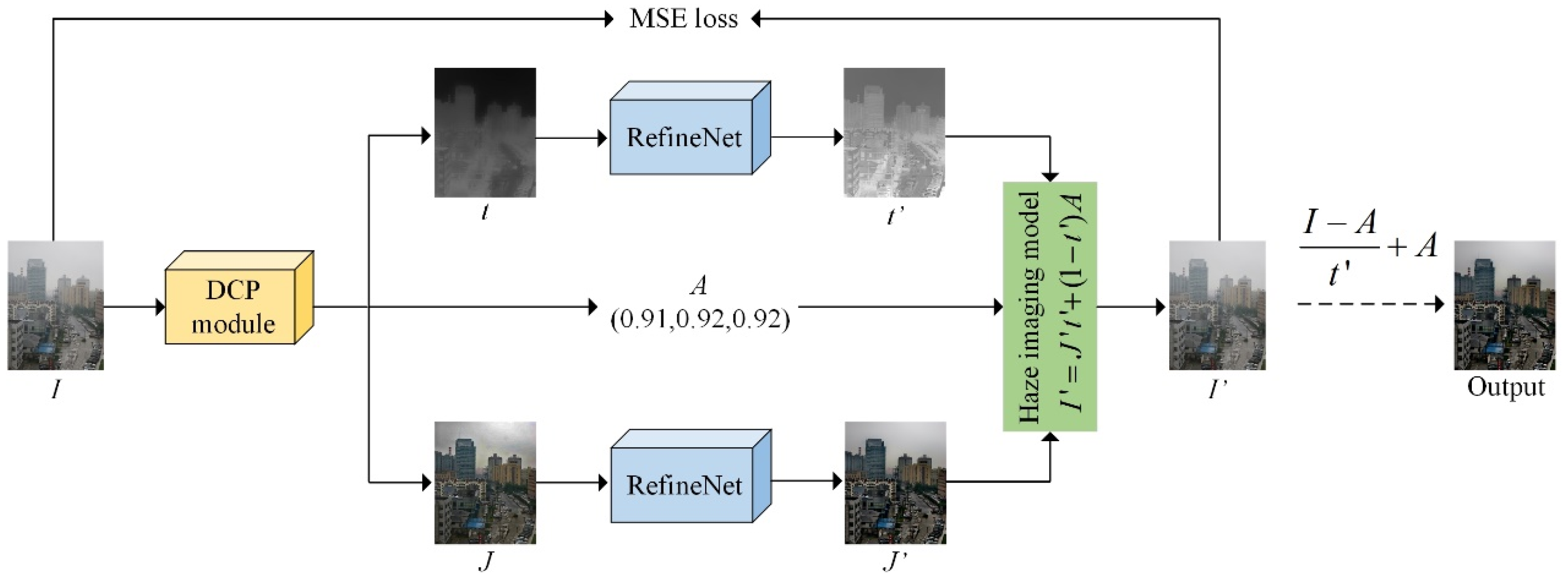
Figure 1 illustrates the overall framework of the proposed zero-shot dehazing network. The hazy image, , is initially fed into the DCP module to obtain the transmission map, , the atmospheric light, , and the initial dehazed result, . Subsequently, and are further refined by two CNN-based refinement networks to obtain and . Using the haze imaging model [37], we regenerate a hazy image using , , and . We ensure that and are consistent using the mean square error (MSE) loss function, allowing the entire network to be trained in a zero-shot manner. Once and are obtained, the haze-free image can be output by reversing the haze imaging model. Overall, the zero-shot learning strategy guarantees the network’s generalizability without requiring dense training data, while the CNN-based RefineNets compensate for the flaws of prior-based dehazing methods.
3.2. The DCP Module
The degradation of images under hazy conditions can be represented by the haze imaging model [37], which is expressed as follows:
where and denote the observed hazy image and its corresponding clean image at pixel location , respectively. represents the atmospheric transmission, which is the fraction of light that reaches the camera after passing through the atmosphere at the same location. represents the global atmospheric light, which refers to the color and intensity of the light scattered by the atmosphere.
In accordance with Equation (1), the estimation of and is essential to derive from . However, this is an ill-posed problem. To address this, the DCP has proven to be one of the most effective image-dehazing priors, as it is observed from the statistics of a large number of hazy and clean images. The dark channel of can be formulated by calculating the minimum intensity in each local region as follows:
where is a local window of size centered at pixel , and denotes the -th color channel intensity at pixel . The DCP implies that the dark channel value in a hazy image is a reliable estimate of the haze intensity. Typically, the dark channel of a clean image tends to be zero, i.e.:
Therefore, by applying the DCP to both sides of Equation (1), we can obtain:
where denotes , i.e., the dark channel of the hazy image . Thus, we can reformate Equation (4) by incorporating Equations (2) and (3) as follows:
Consequently, once is obtained, can be estimated. Typically, is located in the haziest and brightest region of a hazy image. Therefore, we select the top 0.1 percent of the brightest pixels in the dark channel and calculate their average pixel value as . Once and are determined, the clean image can be inferred by inverting Equation (1) as follows:
While the DCP offers a simple and effective way for image dehazing, it may fail in the sky region of an image. Therefore, we use the CNN to refine and for further improvement. Moreover, to compute the dark channel more efficiently and integrate the DCP module into the entire network, we implement the DCP using the max pooling operation [17] with a kernel size of as follows:
By doing so, we separate the input hazy image into three components, , , and , for subsequent refinement.
3.3. RefineNet
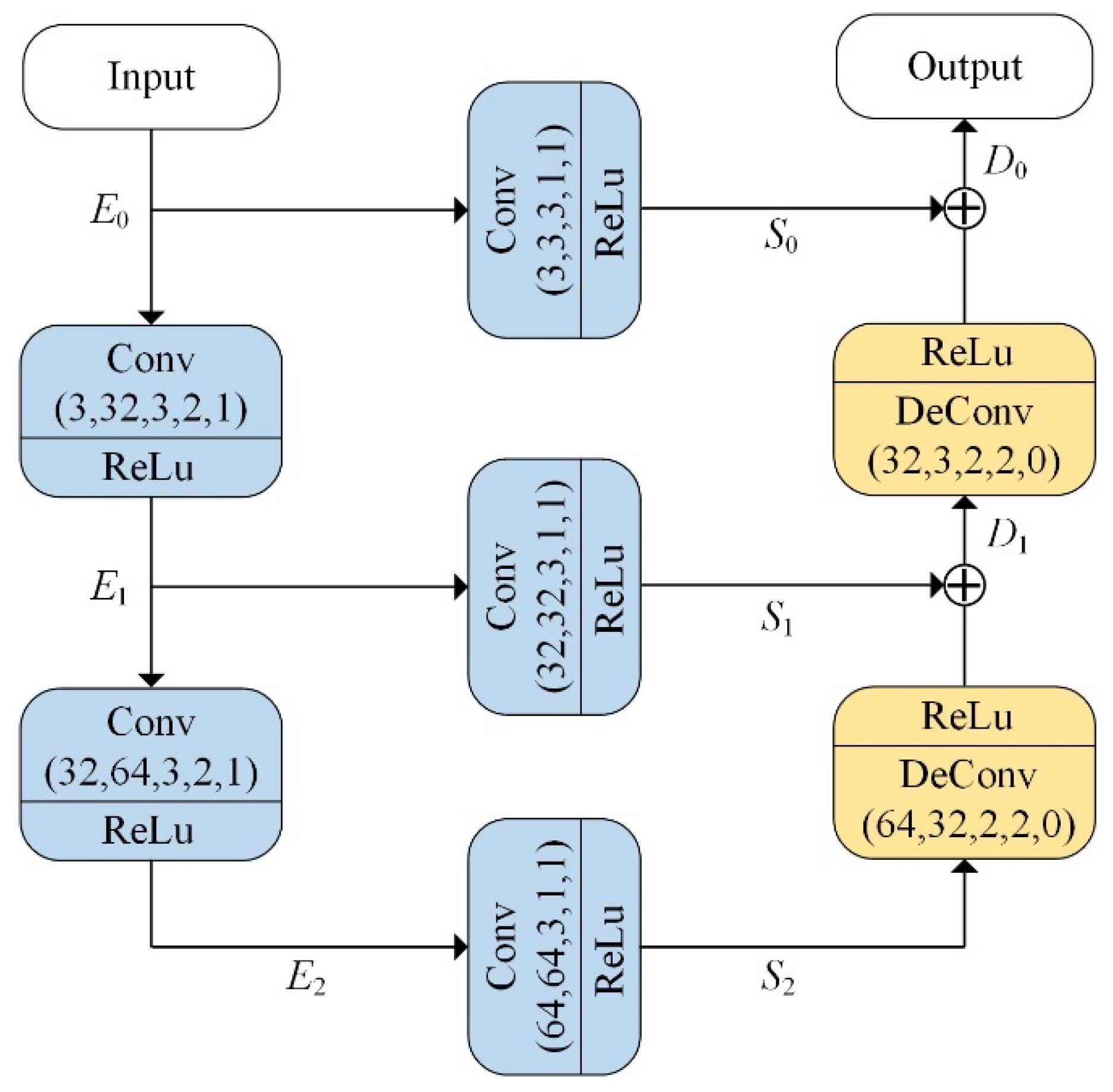
As illustrated in Figure 2, the proposed RefineNet model shown in Figure 1 is a shallow UNet with encoder and decoder architecture. Let , , and denote a convolution layer, a ReLu activation function, and a transposed convolution layer, respectively. The encoder part consists of two layers of , while the decoder part has two layers of . To better preserve the feature information, the encoder and decoder are connected by three layers. In Figure 2, the input channels, output channels, convolution kernel size, strides, and zero-paddings are denoted in brackets below the and layers.
To provide a clearer description of the RefineNet model, we denote the and layers as and , respectively. Therefore, given an input image , the outputs of different layers in the encoder can be expressed as follows:
where . According to the parameters labelled in the layer, the input image is gradually downsampled using strided convolution, while the feature channels are increased. Subsequently, each is passed through a layer to connect with the decoder, as follows:
In contrast to the encoder, the decoder restores the details of the image by adding the feature maps from the encoder and the upsampled feature maps using transposed convolutions, which can be expressed as:
where . Therefore, in the decoder part, the feature maps are gradually upsampled using transposed convolution, while the feature channels are decreased.
To be more specific, consider an input image with a resolution of . The image’s size is gradually downscaled from to , while the feature channels are expanded from 3 to 64. Following this, in the decoder part, the image’s size is upsampled from to , while the feature channels are reduced back to the original 3. Finally, the output of the refine network, denoted by , has the same image size as the input image .
3.4. Loss Function Design
In this section, we provide a detailed description of the loss function. The elaborated loss function, , comprises four terms:
where represents the reconstruction loss, denotes the total variance (TV) loss, is the DCP loss, and represents the minimum pixel intensity loss. and are balancing factors that weigh the contributions of each term in the loss function.
Reconstruction loss. As shown in Figure 1, if the transmission map, atmospheric light, and scene radiance are accurately estimated, the input hazy image, , and the regenerated hazy image, , should be identical. Therefore, we propose the reconstruction loss to minimize the difference between and , as follows:
where indicate loss. The ensures that and are cycle consistent, thereby allowing the entire network to be optimized in a zero-shot learning strategy.
TV loss. The TV loss is incorporated to prevent the model from generating images with high-frequency artifacts or noise and to produce visually pleasing results. It is computed as the sum of the absolute differences between neighboring pixel values in the image. Mathematically, the TV loss can be expressed as:
where and represent the differential operations in the horizontal and vertical dimensions, respectively. Accordingly, the TV loss encourages smoothness in the output images.
DCP loss. As discussed in Section 3.2, the dark channel of a clean image is typically close to zero. Therefore, we use the loss to minimize the dark channel of the recovered , as follows:
where can be computed using Equation (7). By leveraging the DCP loss , the model is optimized to remove haze more effectively.
Minimum pixel intensity loss. Although the DCP loss can effectively remove haze, the dehazed result may have a dark color. Furthermore, if the model is overfitted, the intensity of some image pixels may be clipped to zero, causing the loss of dark details. Therefore, we propose the minimum pixel intensity loss to prevent the image pixels from being over-saturated due to the minimization of . The is defined as follows:
where represents the image pixel, and denotes the total number of image pixels. The ensures that the pixel intensity of and is not lower than 0.1, compensating for the over-clipping of pixel intensity caused by .
3.5. Functionality of Modules in the Dehazing Framework
In this section, we describe the functionality of the proposed dehazing framework’s various modules. The dehazing network consists primarily of two components: a DCP module and two RefineNets. The RS hazy image is initially preprocessed by the DCP module, and its outputs are then refined by the RefineNets module.
The DCP module is implemented with two advantages: (1) The DCP module separates the hazy input into three components (dehazed image, transmission map, and atmospheric light) based on the haze imaging model [37], which guarantees the design of the reconstruction loss function. (2) The initial dehazed image contributes to the design of the lightweight RefineNet architecture and improves the efficiency of subsequent zero-shot training.
Although the DCP is effective at removing haze, it is inapplicable to white regions and produces undesirable artifacts. To rectify the defects, the CNN-based RefineNets is implemented. The well-designed loss function facilitates the network’s zero-shot learning. Ultimately, the proposed dehazing framework offers three benefits: (1) effective haze removal, (2) excellent generalizability, and (3) rapid zero-shot training speed.
4. Experiments and Discussions
4.1. Experimental Settings
In this section, we provide details about the experimental settings, including the datasets, training procedures, and baselines.
Datasets. We evaluate our proposed method on both real-world and synthetic hazy image datasets. For real-world hazy images, we use the aerial RS hazy images from Zhang et al.’s work [38] and Flickr for qualitative analysis. For quantitative evaluation, we synthesize uniform and non-uniform RS hazy images. We select 90 non-uniform RS hazy images with different haze densities from the SateHaze1k dataset [39]. To generate the uniform RS hazy dataset, we use images from the DeepGlobe road extraction dataset [40] and apply the haze imaging model in Equation (1), with the atmospheric light, , and transmission map, , uniformly defined between and , respectively. Eventually, we have 90 images as the uniform RS hazy datasets, which are also chosen for the high-level vision task analysis in Section 4.5.
Training details. We train the proposed model using the PyTorch toolbox on the Ubuntu 20.04 LTS operating system. We use the Adam optimizer with a fixed learning rate of 0.0001. As a zero-shot dehazing method, we train the model for each image for approximately 500 iterations to obtain the final result. We empirically set the balancing parameters and in Equation (11) to and , respectively. The training is performed on a PC with an i7-9700F processor @3.00 GHz, 24 GB RAM, and a NVIDIA RTX 3080 GPU. We present the training details of each iteration in Algorithm 1.
| Algorithm 1: Zero-shot training details at each iteration, where indicates the DCP module for preliminary dehazing, and refer to the RefineNets for transmission map and initial dehazed image . | |
| Input: Initialized RefineNet , hazy image , max training iterations , balancing parameters and . | |
| Output: Dehazed image . | |
| 1: | while do |
| 2: | obtain initial dehazed image, , transmission map, , atmospheric light, , by |
| 3: | obtain refined dehazed image, , by |
| 4: | obtain refined transmission map, , by |
| 5: | obtain reconstructed hazy image, , by Equation (1), |
| 6: | obtain reconstruction loss, , by Equation (12) |
| 7: | obtain TV loss, , by Equation (13) |
| 8: | obtain DCP loss, , by Equation (14) |
| 9: | obtain minimum pixel intensity loss, , by Equation (15) |
| 10: | back propagate loss function, , by |
| 11: | |
| 12: | end while |
| 13: | obtain final dehazed output by |
Baselines. In order to verify the performance of our proposed method, we compared it to various state-of-the-art (SOTA) dehazing methods, including traditional, learning-based, and zero-shot dehazing methods. Table 1 presents a classification of each method according to its dehazing type and a brief explanation for better comprehension. The traditional dehazing methods encompass a prior-based method (DCP [8]) and enhancement-based methods (CEEF [6] and FADE [41]). The learning-based methods include supervised learning-based methods (DehazeFlow [42], SRKTDN [43], and DWGAN [44]), a semi-supervised learning-based method (RefineDNet [17]), and an unsupervised learning-based method (USIDNet [45]). The zero-shot dehazing methods evaluated are ZID [14], DDIP [35], YOLY [13], ZIR [16], and our proposed method. As there is no ground truth image available for a real-world RS hazy image, we use the result obtained from the dehazing tool of Photoshop 2021 as a reference. To assure a fair comparison, all methods were tested using MATLAB or PyCharm in the same software and hardware environment. For learning-based methods, we chose the default configurations from the literature and used their pre-trained models for a more accurate generalizability comparison. For zero-shot dehazing techniques, the models were trained with their default parameters. For ZID [14], DDIP [35], YOLY [13], and ZIR [16], the training iterations are 500, 4000, 500, and 10,000, respectively. We quantitatively analyzed the dehazing performance using three metrics, namely, peak signal-to-noise ratio (PSNR), structural similarity (SSIM), and learned perceptual image patch similarity (LPIPS) [46]. The PSNR and SSIM metrics are commonly used to evaluate image quality, while LPIPS is a metric based on a deep neural network for assessing the perceptual similarity between two images.
4.2. Results for Real-World RS Hazy Images
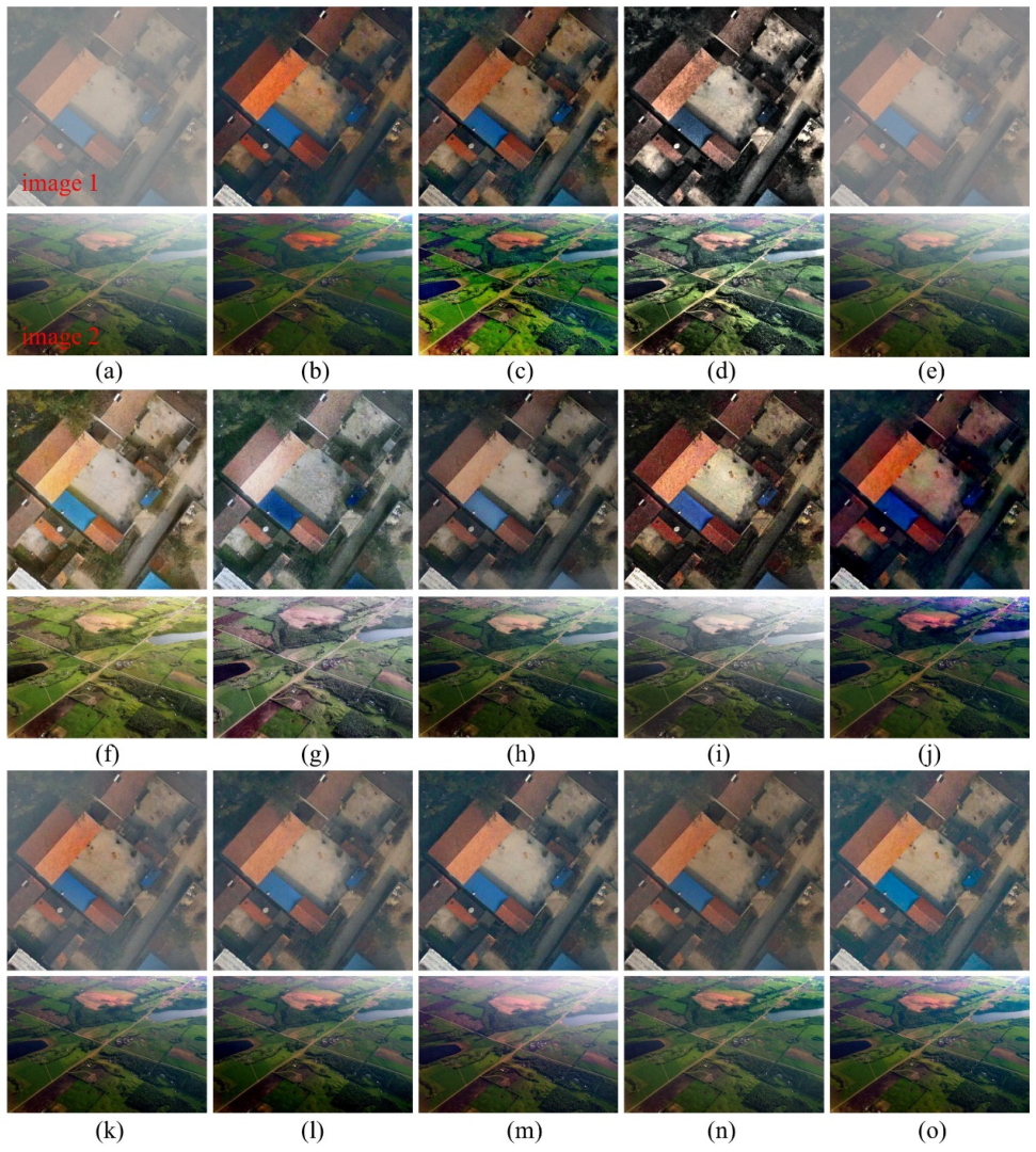
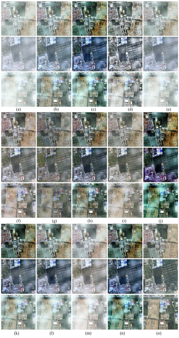
In this section, we present a qualitative comparison of the dehazing performance of different methods using real-world RS hazy images. The results are depicted in Figure 3. Figure 3a shows two aerial hazy images labeled as “image 1” and “image 2,”, respectively. These images were selected from Zhang et al.’s work [38] and Flickr. Figure 3b–o show the dehazed results obtained using various methods. The original hazy images appear blurry and have low contrast. However, after applying the dehazing process, the image quality improves significantly. Nonetheless, different methods remove haze to varying extents. DehazeFlow, as a supervised learning-based method, fails to remove haze properly in Figure 3e, suggesting poor generalizability to real-world RS image dehazing. The result obtained by ZID in Figure 3j exhibits an apparent color shift on the roof of “image 1.” FADE and USIDNet have over-enhancement issues, as can be seen in “image 1” of Figure 3d,i, respectively. In Figure 3f,g, SRKTDN and DWGAN produce unnatural-looking dehazed images with color saturation loss. DCP and RefineDNet show good dehazing performance, but the results in Figure 3b,h display a slight dark color. CEEF delivers a well-dehazed image with full detailed information in Figure 3c, although “image 1” suffers from slight color distortion. All zero-shot dehazing methods, except for ZID, generate natural and pleasing dehazed images. However, in Figure 3k,j,m, DDIP, YOLY, and ZIR exhibit undesired bright flares on the top right of “image 2.” Our proposed method, as shown in Figure 3n, outperforms the other dehazing methods in terms of dehazing and color consistency when compared to the reference result by Photoshop in Figure 3o. Therefore, the embedded DCP module assures that our network has effective haze removal ability, while the RefineNet corrects the DCP’s shortcomings. Moreover, the zero-shot learning manner guarantees the good generalizability of our model while processing the complex real-world RS hazy images.
4.3. Results on Synthetic Uniform RS Hazy Images
Figure 4 shows the dehazed results obtained on synthetic uniform RS hazy images. Figure 4a presents the hazy image, Figure 4b–n show the dehazed results using different methods, and Figure 4o displays the ground truth image. Among the evaluated methods, ZID produces the worst results with severe color shift (Figure 4j), while FADE and USIDNet exhibit obvious over-enhancement problems (Figure 4d,i). DehazeFlow, DDIP, and YOLY fail to remove haze adequately, as shown in Figure 4e,k,l, respectively. Although DCP and RefineDNet can thoroughly remove haze, the results in Figure 4b,h display a slightly uneven dark color. SRKTDN, DWGAN, and ZIR show good haze removal ability, but the recovered images in Figure 4f,g,m exhibit slight color distortion with saturation loss. Using the ground truth image in Figure 4o as a reference, CEEF and our proposed method produce better results. Therefore, our method is superior to most other methods when processing RS images with uniform haze.
To evaluate the dehazing performance quantitatively, we calculated the PSNR, SSIM, and LPIPS values using the dehazed image and the ground truth. Higher PSNR and SSIM values indicate better results, while lower LPIPS values signify better perceptual similarity. Table 2 presents the quantitative dehazing evaluation results for RS images with uniform haze. The dehazing methods are categorized, and the best result for each category and each metric is marked in bold. As shown in Table 2, for the traditional dehazing category, DCP obtains the best score for SSIM and LPIPS metrics, while the CEEF obtains the best value for the PSNR metric. DehazeFlow obtains the best results for all three metrics in the learning-based category.
Our proposed method exhibits outstanding performance in the zero-shot dehazing category, ranking first in both SSIM and the LPIPS metrics, and second in the PSNR. Notably, our approach outperforms all dehazing methods in both traditional and learning-based categories for all three evaluation metrics. Compared to the existing DCP approach, our proposed method achieves an improvement of 2.04 dB and 0.11 for PSNR and SSIM, respectively. Moreover, our method surpasses RefineDNet, which has a similar network architecture, by gaining an increase of 2.93 dB and 0.14 for PSNR and SSIM, respectively. These results confirm that our approach represents a significant improvement over the SOTA methods in uniform dehazing.
4.4. Results for Synthetic Non-Uniform RS Hazy Images
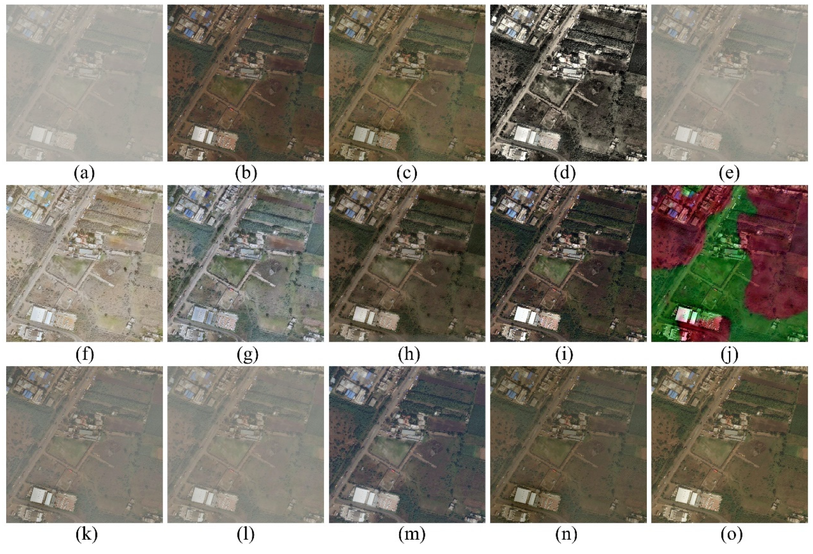
We used the SateHaze1k [39] dataset, a synthetic non-uniform hazy dataset containing 1200 pairs of hazy/clean RS images with three haze densities—thin, moderate, and thick—for non-uniform dehazing evaluation. We randomly selected 30 hazy images from each haze density, resulting in a total of 90 hazy images as our test dataset. Figure 5 presents the comparative dehazing results for SateHaze1k. Figure 5a displays the input hazy images with different haze densities labeled by red fonts. Figure 5b–n show the dehazed results using different methods, and Figure 5o provides the ground truth for reference. As shown in Figure 5, most dehazing methods can effectively remove thin haze, except for DehazeFlow (Figure 5e) and ZIR (Figure 5m). However, ZID produces over-enhancement and color distortion. Among traditional dehazing methods, DCP, CEEF, and FADE show similar performance in processing images with different haze densities, but FADE exhibits over-enhancement in Figure 5d. For thick hazy images, learning-based methods (except DehazeFlow) provide visually better results than other dehazing methods. In the zero-shot dehazing category, our proposed method outperforms other methods in terms of haze removal and color preservation.
Table 3 displays the results of the quantitative evaluation on the SateHaze1k [39] dataset. We calculated the PSNR, SSIM, and LPIPS metrics for each haze density, and the average value is provided. As shown in Table 3, DCP obtains the best results in the traditional dehazing category, while the performance of different learning-based dehazing methods varies significantly. In the zero-shot dehazing category, our proposed method obtains the best results in all metrics and all haze densities, except for thin haze density, for which it achieved the second-best PSNR value. Furthermore, the average performance of our proposed method across the three evaluation metrics exceeds that of all dehazing methods in the traditional category and outperforms most methods in the learning-based category. These results highlight the competitive non-uniform haze removal ability of our proposed dehazing approach.
4.5. Application to a High-Level Vision Task
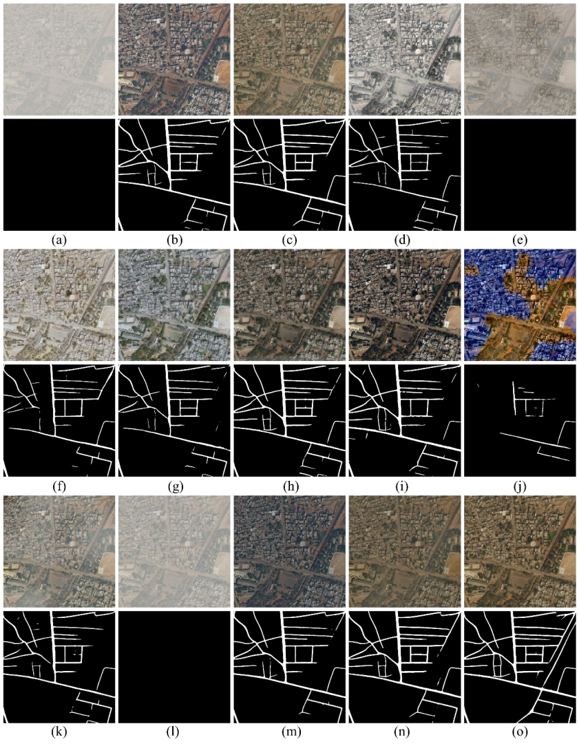
Dehazing is a crucial image preprocessing step for high-level computer vision tasks. In this regard, we compared the road extraction results of D-LinkNet [47] using dehazed images generated by different dehazing methods, as presented in Figure 6. The first and second rows of Figure 6 are the input and corresponding output images of the D-LinkNet road extraction algorithm, respectively. Figure 6a shows the original hazy image, while Figure 6b–n present the results obtained using different dehazing methods. Figure 6o is provided as the ground truth for reference. As demonstrated in Figure 6a, the D-LinkNet algorithm fails to work effectively due to the interference of haze in the original hazy image. Although DehazeFlow and YOLY have removed some haze, the dehazed results are not sufficient for D-LinkNet to extract any road information, as presented in Figure 6e,l, respectively. The dehazed image generated by ZID has severe color distortion, resulting in D-LinkNet extracting only a few roads. In comparison to other dehazing methods, our proposed method generates more continuous road lines, and the extracted road masks are closer to the reference ground truth. Therefore, our proposed method demonstrates superior performance as an image preprocessing step for D-LinkNet.
To quantitatively evaluate road extraction accuracy, we calculated four commonly used evaluation metrics in object detection and segmentation tasks: Precision, Recall, IoU, and F1-score. The four metrics are defined as follows:
Here, , , and denote true positives, false positives, and false negatives, respectively. The F1-score is a weighted harmonic mean of Precision and Recall, which accounts for both false positives and false negatives. To evaluate the road extraction accuracy, we used a synthetic uniform hazy dataset consisting of 90 images as the input for different dehazing methods. The dehazed images were processed using D-LinkNet to extract roads, and the road extraction accuracy was calculated using the extracted results and the ground truth road masks.
Table 4 shows that the road extraction accuracy of D-LinkNet using clear images as the input is significantly better than that using hazy images, indicating that haze has a severe negative impact on D-LinkNet’s performance. Table 5 presents the road extraction accuracy comparison for different dehazing methods. It is evident that the DCP, SRKTDN, and our proposed method achieved the best results for the four metrics in the traditional, learning-based, and zero-shot dehazing categories, respectively. Moreover, our proposed method outperforms the other methods in traditional and learning-based categories for the four metrics, demonstrating its superior performance.
4.6. Discussion
In this section, we discuss the efficacy of the proposed dehazing framework through an ablation study, a convergency test, network size comparison, and a training time complexity analysis.
Ablation study. The effectiveness of our proposed loss function is demonstrated through an ablation study, where we remove part of the loss function in Equation (11) and compare the dehazed results. The results of the ablation study are illustrated in Figure 7. As shown, the dehazed result using our proposed loss function (see Figure 7f) is superior to that of removing any part of the loss function. Removing the reconstruction loss causes the entire dehazing framework not to be cycle-inconsistent, resulting in over-enhancement. The TV loss encourages the model to smooth out the details in an image. Therefore, removing the TV loss leads to undesired noise in the sky region in Figure 7c. The DCP loss helps the model remove haze properly, but may result in a dark color. The model without the DCP loss has poor dehazing performance, as shown in Figure 7d. On the other hand, the minimum pixel intensity loss prevents the image pixels from being oversaturated. Thus, removing the minimum pixel intensity loss results in most of the dark details being lost, as shown in Figure 7e. Therefore, the proposed loss function is effective in producing pleasing results for the dehazing framework.
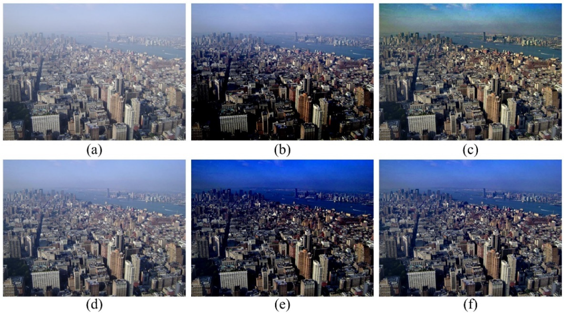
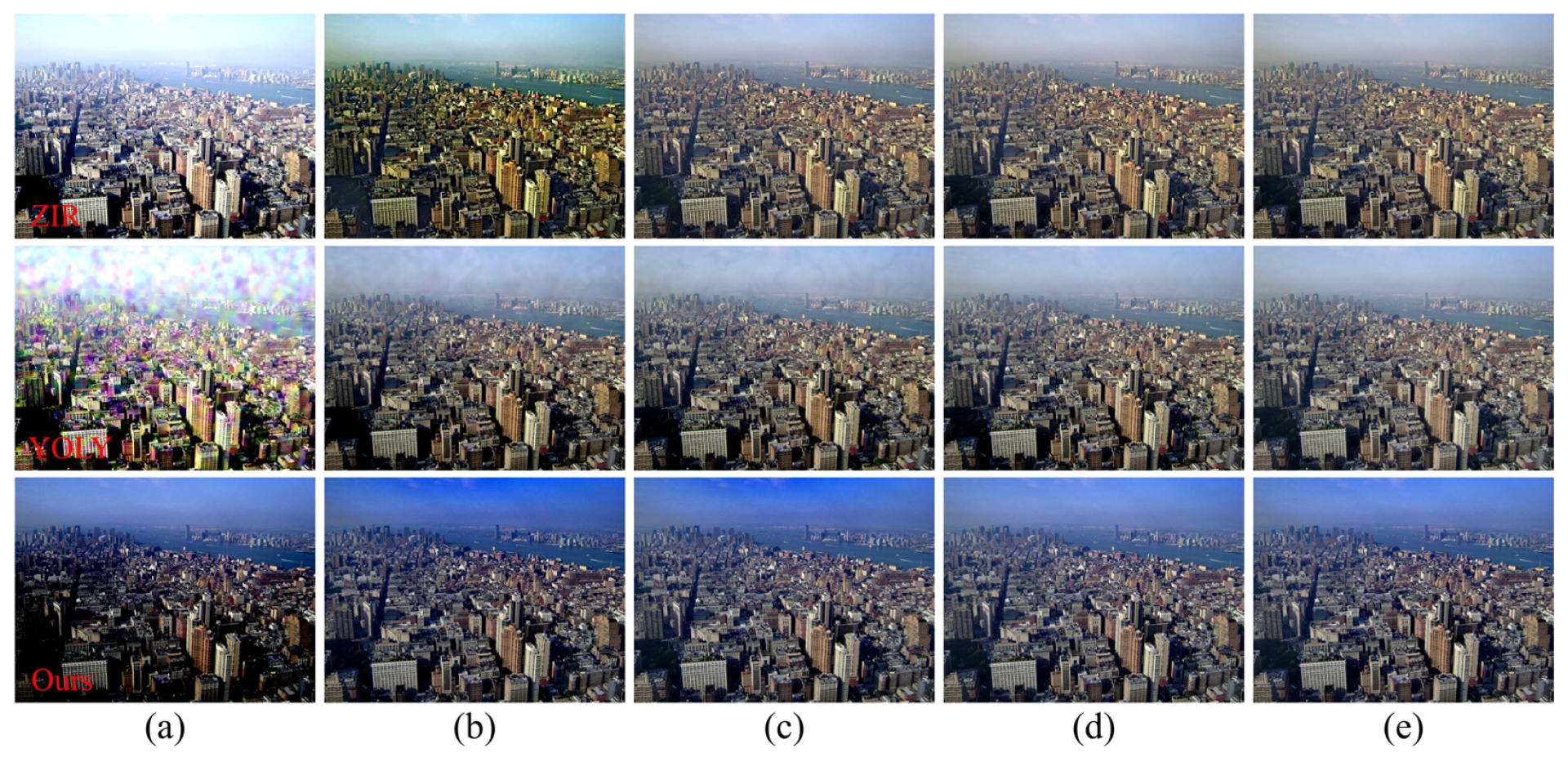
Convergency test. During the training process of a zero-shot dehazing technique, an optimally designed network generates output by minimizing the loss function. However, distinct methods require varying numbers of training steps to produce satisfactory haze-free images, leading to differences in training efficiency. For instance, YOLY [13] necessitates 500 steps, while ZIR [16] demands 10,000 steps to reach the final output. Consequently, we compare the dehazed outcomes produced by various zero-shot approaches during the different training steps to demonstrate the network’s convergency. The results are illustrated in Figure 8. At the start of the training process (step 1 in Figure 8a), YOLY’s output exhibits significant unwanted flares, which complicates the network convergence for generating superior dehazed results in subsequent training phases. In the case of ZIR, the network produces dehazed outcomes with substantial color shifts until step 100, and the output quality improves at a slow rate, indicating suboptimal convergence efficiency. In contrast, the proposed method benefits from the integrated DCP pre-dehazing module, which eliminates most haze in the initial step 1, despite the image appearing darker due to the DCP’s influence. By step 100, our model rectifies the dark color issues through the RefineNet model, and the model converges with minimal enhancements to the dehazed image’s quality. As a result, our zero-shot dehazing technique outperforms others in terms of convergence efficiency.
Network size comparison. Since zero-shot dehazing methods train the model for each degraded image, the training time complexity is important when evaluating the performance of the algorithm. A complex network architecture is not suitable for zero-shot image dehazing because it will significantly increase the training time complexity. Therefore, we compared the network size of different zero-shot dehazing methods to show the superiority of our method. As shown in Table 6, since the ZID and YOLY have similar network architecture, they have comparable network sizes and are substantially larger than those of the other methods. The DDIP, ZIR, and our method all possess a relatively lightweight network, but our method is the lightest.
Training time complexity analysis. In order to further evaluate the training efficiency of a zero-shot dehazing method, we compared the execution time of various methods for processing a 512 × 512 pixel RS hazy image. According to Table 7, the ZIR has the lowest training efficacy, requiring more than five minutes to infer a haze-free image. Due to their similar network structures, the ZID and YOLY have a comparable training time complexity. As described in Section 3.5, thanks to the pre-dehazing DCP module and a lightweight network design, our proposed method has the highest training efficiency and outperforms all other methods by a significant margin.
5. Conclusions
This paper presents a zero-shot dehazing network that combines the strengths of prior-based dehazing and CNN. Initially, the RS hazy image undergoes processing via the DCP based module to obtain the transmission map, atmospheric light, and initial dehazed image. Two shallow UNet-based CNNs are then proposed to refine the transmission map and the initial dehazed image, compensating for the DCP’s failure cases. Another hazy image is generated using the atmospheric light, refined transmission map, and the refined dehazed image based on the haze imaging model. The proposed loss function ensures that the network regenerates a hazy image that is similar to the input one, allowing the whole dehazing network to be trained in a zero-shot manner. Overall, the proposed dehazing network has two advantages: (1) the DCP is embedded within the CNN to enhance dehazing performance, mitigate the inherent limitations of DCP, and improve overall training efficacy; and (2) the zero-shot learning process improves the network’s generalizability without the need for large-scale training data collections. In the experiments, real-world and synthetic RS hazy images were selected to verify the effectiveness of the proposed method. The qualitative and quantitative evaluation results indicate that our method outperforms many other dehazing methods in processing both uniform and non-uniform RS hazy images. Furthermore, the proposed method’s superiority is demonstrated in a high-level vision task (road extraction).
Author Contributions
Conceptualization, J.W. and Y.W.; methodology, J.W. and K.Y.; software, J.W. and Y.C.; validation, Y.W. and K.Y.; data curation, J.W. and Y.C.; funding acquisition, J.W. and Y.W.; writing—original draft preparation, J.W.; writing—review and editing, J.W., Y.C., K.Y., Y.W. and L.C.; supervision, Y.W., L.C. and K.Y. All authors have read and agreed to the published version of the manuscript.
Funding
This research is supported by the National Natural Science Foundation of China (U1805262, 61901117, 62201152); the special Funds of the Central Government Guiding Local Science and Technology Development (2021L3010); Key provincial scientific and technological innovation projects (2021G02006); the Natural Science Foundation of Fujian Province, China (2022J01169, 2020J01157); the Scientific Research Project of Fujian Jiangxia University (JXZ2021013); and the Education and Scientific Research Project for Middle-aged and Young Teachers in Fujian Province (JAT200370).
Data Availability Statement
The data that support the findings of this study are available on request from the corresponding author.
Conflicts of Interest
All authors declare no conflict of interest.
References
- Zhang, L.; Zhang, L. Artificial intelligence for remote sensing data analysis: A review of challenges and opportunities. IEEE Geosci. Remote Sens. Mag. 2022, 10, 2–27. [Google Scholar] [CrossRef]
- Yang, F.; Guo, J.; Tan, H.; Wang, J. Automated extraction of urban water bodies from ZY-3 multi-spectral imagery. Water 2017, 9, 144. [Google Scholar] [CrossRef]
- Lian, R.; Zhang, Z.; Zou, C.; Huang, L. An Effective Road Centerline Extraction Method From VHR. IEEE Geosci. Remote Sens. Lett. 2022, 19, 69052025. [Google Scholar] [CrossRef]
- Yang, K.; Xia, G.-S.; Liu, Z.; Du, B.; Yang, W.; Pelillo, M.; Zhang, L. Asymmetric siamese networks for semantic change detection in aerial images. IEEE Trans. Geosci. Remote Sens. 2021, 60, 5609818. [Google Scholar] [CrossRef]
- Zhu, D.; Wang, B.; Zhang, L. Airport target detection in remote sensing images: A new method based on two-way saliency. IEEE Geosci. Remote Sens. Lett. 2015, 12, 1096–1100. [Google Scholar]
- Liu, X.; Li, H.; Zhu, C. Joint contrast enhancement and exposure fusion for real-world image dehazing. IEEE Trans. Multimed. 2021, 24, 3934–3946. [Google Scholar] [CrossRef]
- Khan, H.; Sharif, M.; Bibi, N.; Usman, M.; Haider, S.A.; Zainab, S.; Shah, J.H.; Bashir, Y.; Muhammad, N. Localization of radiance transformation for image dehazing in wavelet domain. Neurocomputing 2020, 381, 141–151. [Google Scholar] [CrossRef]
- He, K.; Sun, J.; Tang, X. Single image haze removal using dark channel prior. IEEE Trans. Pattern Anal. Mach. Intell. 2010, 33, 2341–2353. [Google Scholar]
- Zhu, Q.; Mai, J.; Shao, L. A fast single image haze removal algorithm using color attenuation prior. IEEE Trans. Image Process. 2015, 24, 3522–3533. [Google Scholar]
- Berman, D.; Treibitz, T.; Avidan, S. Single image dehazing using haze-lines. IEEE Trans. Pattern Anal. Mach. Intell. 2018, 42, 720–734. [Google Scholar] [CrossRef] [PubMed]
- Qin, X.; Wang, Z.; Bai, Y.; Xie, X.; Jia, H. FFA-Net: Feature fusion attention network for single image dehazing. In Proceedings of the AAAI Conference on Artificial Intelligence, New York, NY, USA, 7–12 February 2020; Volume 34, pp. 11908–11915. [Google Scholar]
- Chen, W.-T.; Fang, H.-Y.; Ding, J.-J.; Kuo, S.-Y. PMHLD: Patch map-based hybrid learning DehazeNet for single image haze removal. IEEE Trans. Image Process. 2020, 29, 6773–6788. [Google Scholar] [CrossRef]
- Li, B.; Gou, Y.; Gu, S.; Liu, J.Z.; Zhou, J.T.; Peng, X. You only look yourself: Unsupervised and untrained single image dehazing neural network. Int. J. Comput. Vis. 2021, 129, 1754–1767. [Google Scholar] [CrossRef]
- Li, B.; Gou, Y.; Liu, J.Z.; Zhu, H.; Zhou, J.T.; Peng, X. Zero-shot image dehazing. IEEE Trans. Image Process. 2020, 29, 8457–8466. [Google Scholar] [CrossRef] [PubMed]
- Wei, J.; Wu, Y.; Chen, L.; Yang, K.; Lian, R. Zero-Shot Remote Sensing Image Dehazing Based on a Re-Degradation Haze Imaging Model. Remote Sens. 2022, 14, 5737. [Google Scholar] [CrossRef]
- Kar, A.; Dhara, S.K.; Sen, D.; Biswas, P.K. Zero-Shot Single Image Restoration Through Controlled Perturbation of Koschmieder’s Model. In Proceedings of the IEEE/CVF Conference on Computer Vision and Pattern Recognition, Nashville, TN, USA, 20–25 June 2021; pp. 16205–16215. [Google Scholar]
- Zhao, S.; Zhang, L.; Shen, Y.; Zhou, Y. RefineDNet: A weakly supervised refinement framework for single image dehazing. IEEE Trans. Image Process. 2021, 30, 3391–3404. [Google Scholar] [CrossRef]
- Wang, W.; Yuan, X.; Wu, X.; Liu, Y. Fast image dehazing method based on linear transformation. IEEE Trans. Multimed. 2017, 19, 1142–1155. [Google Scholar] [CrossRef]
- Ni, W.; Gao, X.; Wang, Y. Single satellite image dehazing via linear intensity transformation and local property analysis. Neurocomputing 2016, 175, 25–39. [Google Scholar] [CrossRef]
- Cho, Y.; Jeong, J.; Kim, A. Model-assisted multiband fusion for single image enhancement and applications to robot vision. IEEE Robot. Autom. Lett. 2018, 3, 2822–2829. [Google Scholar]
- Han, Y.; Yin, M.; Duan, P.; Ghamisi, P. Edge-preserving filtering-based dehazing for remote sensing images. IEEE Geosci. Remote Sens. Lett. 2021, 19, 8019105. [Google Scholar] [CrossRef]
- Singh, D.; Kumar, V.; Kaur, M. Single image dehazing using gradient channel prior. Appl. Intell. 2019, 49, 4276–4293. [Google Scholar] [CrossRef]
- Han, J.; Zhang, S.; Fan, N.; Ye, Z. Local patchwise minimal and maximal values prior for single optical remote sensing image dehazing. Inf. Sci. 2022, 606, 173–193. [Google Scholar] [CrossRef]
- Chen, T.; Liu, M.; Gao, T.; Cheng, P.; Mei, S.; Li, Y. A Fusion-Based Defogging Algorithm. Remote Sens. 2022, 14, 425. [Google Scholar] [CrossRef]
- Dharejo, F.A.; Zhou, Y.; Deeba, F.; Jatoi, M.A.; Du, Y.; Wang, X. A remote-sensing image enhancement algorithm based on patch-wise dark channel prior and histogram equalisation with colour correction. IET Image Process. 2021, 15, 47–56. [Google Scholar] [CrossRef]
- Huang, Y.; Chen, X. Single Remote Sensing Image Dehazing Using a Dual-Step Cascaded Residual Dense Network. In Proceedings of the 2021 IEEE International Conference on Image Processing (ICIP), Anchorage, AK, USA, 19–22 September 2021; pp. 3852–3856. [Google Scholar]
- Shi, Z.; Shao, S.; Zhou, Z. A saliency guided remote sensing image dehazing network model. IET Image Process. 2022, 16, 2483–2494. [Google Scholar] [CrossRef]
- Jiang, B.; Chen, G.; Wang, J.; Ma, H.; Wang, L.; Wang, Y.; Chen, X. Deep Dehazing Network for Remote Sensing Image with Non-Uniform Haze. Remote Sens. 2021, 13, 4443. [Google Scholar] [CrossRef]
- Engin, D.; Genç, A.; Ekenel, H.K. Cycle-dehaze: Enhanced cyclegan for single image dehazing. In Proceedings of the IEEE Conference on Computer Vision and Pattern Recognition Workshops, Salt Lake City, UT, USA, 18–22 June 2018; pp. 825–833. [Google Scholar]
- Zheng, Y.; Su, J.; Zhang, S.; Tao, M.; Wang, L. Dehaze-AGGAN: Unpaired Remote Sensing Image Dehazing Using Enhanced Attention-Guide Generative Adversarial Networks. IEEE Trans. Geosci. Remote Sens. 2022, 60, 5630413. [Google Scholar] [CrossRef]
- Chen, X.; Huang, Y. Memory-Oriented Unpaired Learning for Single Remote Sensing Image Dehazing. IEEE Geosci. Remote Sens. Lett. 2022, 19, 3511705. [Google Scholar] [CrossRef]
- Li, L.; Dong, Y.; Ren, W.; Pan, J.; Gao, C.; Sang, N.; Yang, M.H. Semi-supervised image dehazing. IEEE Trans. Image Process. 2019, 29, 2766–2779. [Google Scholar] [CrossRef]
- Bie, Y.; Yang, S.; Huang, Y. Single Remote Sensing Image Dehazing using Gaussian and Physics-Guided Process. IEEE Geosci. Remote Sens. Lett. 2022, 19, 3512405. [Google Scholar] [CrossRef]
- Li, Y.; Chen, H.; Miao, Q.; Ge, D.; Liang, S.; Ma, Z.; Zhao, B. Image Hazing and Dehazing: From the Viewpoint of Two-Way Image Translation With a Weakly Supervised Framework. IEEE Trans. Multimed. 2022. [Google Scholar] [CrossRef]
- Gandelsman, Y.; Shocher, A.; Irani, M. “double-dip”: Unsupervised image decomposition via coupled deep-image-priors. In Proceedings of the IEEE/CVF Conference on Computer Vision and Pattern Recognition, Long Beach, CA, USA, 15–20 June 2019; pp. 11026–11035. [Google Scholar]
- Ulyanov, D.; Vedaldi, A.; Lempitsky, V. Deep image prior. In Proceedings of the IEEE Conference on Computer Vision and Pattern Recognition, Salt Lake City, UT, USA, 18–22 June 2018; pp. 9446–9454. [Google Scholar]
- Singh, D.; Kumar, V. A comprehensive review of computational dehazing techniques. Arch. Comput. Methods Eng. 2019, 26, 1395–1413. [Google Scholar] [CrossRef]
- Zhang, K.; Ma, S.; Zheng, R.; Zhang, L. UAV Remote Sensing Image Dehazing Based on Double-Scale Transmission Optimization Strategy. IEEE Geosci. Remote Sens. Lett. 2022, 19, 6516305. [Google Scholar] [CrossRef]
- Huang, B.; Zhi, L.; Yang, C.; Sun, F.; Song, Y. Single satellite optical imagery dehazing using SAR image prior based on conditional generative adversarial networks. In Proceedings of the IEEE/CVF Winter Conference on Applications of Computer Vision, Snowmass Village, CO, USA, 1–5 March 2020; pp. 1806–1813. [Google Scholar]
- Demir, I.; Koperski, K.; Lindenbaum, D.; Pang, G.; Huang, J.; Basu, S.; Hughes, F.; Tuia, D.; Raskar, R. Deepglobe 2018: A challenge to parse the earth through satellite images. In Proceedings of the IEEE Conference on Computer Vision and Pattern Recognition Workshops, Salt Lake City, UT, USA, 18–22 June 2018; pp. 172–181. [Google Scholar]
- Li, Z.; Zheng, X.; Bhanu, B.; Long, S.; Zhang, Q.; Huang, Z. Fast region-adaptive defogging and enhancement for outdoor images containing sky. In Proceedings of the 2020 25th International Conference on Pattern Recognition (ICPR), Milan, Italy, 10–15 January 2021; pp. 8267–8274. [Google Scholar]
- Li, H.; Li, J.; Zhao, D.; Xu, L. DehazeFlow: Multi-scale Conditional Flow Network for Single Image Dehazing. In Proceedings of the 29th ACM International Conference on Multimedia, Virtual Event China, 20–24 October 2021; pp. 2577–2585. [Google Scholar]
- Chen, T.; Fu, J.; Jiang, W.; Gao, C.; Liu, S. SRKTDN: Applying super resolution method to dehazing task. In Proceedings of the IEEE/CVF Conference on Computer Vision and Pattern Recognition, Nashville, TN, USA, 20–25 June 2021; pp. 487–496. [Google Scholar]
- Fu, M.; Liu, H.; Yu, Y.; Chen, J.; Wang, K. DW-GAN: A discrete wavelet transform GAN for nonhomogeneous dehazing. In Proceedings of the IEEE/CVF Conference on Computer Vision and Pattern Recognition, Nashville, TN, USA, 20–25 June 2021; pp. 203–212. [Google Scholar]
- Li, J.; Li, Y.; Zhuo, L.; Kuang, L.; Yu, T. USID-Net: Unsupervised Single Image Dehazing Network via Disentangled Representations. IEEE Trans. Multimed. 2022. [Google Scholar] [CrossRef]
- Zhang, R.; Isola, P.; Efros, A.A.; Shechtman, E.; Wang, O. The unreasonable effectiveness of deep features as a perceptual metric. In Proceedings of the IEEE Conference on Computer Vision and Pattern Recognition Workshops, Salt Lake City, UT, USA, 18–22 June 2018; pp. 586–595. [Google Scholar]
- Zhou, L.; Zhang, C.; Wu, M. D-LinkNet: LinkNet with pretrained encoder and dilated convolution for high resolution satellite imagery road extraction. In Proceedings of the IEEE Conference on Computer Vision and Pattern Recognition Workshops, Salt Lake City, UT, USA, 18–22 June 2018; pp. 182–186. [Google Scholar]
Figure 1.
The overall framework of the proposed zero-shot dehazing network. Initial outputs and from the DCP module are deemed insufficient. Yet, after refining them using two RefineNets, a more detailed version of , i.e., , is generated, and the issue of over-enhancement in the sky region of is resolved, resulting in the enhanced output .

Figure 2.
The architecture of the RefineNet model.

Figure 3.
The results on real-world aerial RS hazy images. (a) Hazy image; (b) DCP [8]; (c) CEEF [6]; (d) FADE [41]; (e) DehazeFlow [42]; (f) SRKTDN [43]; (g) DWGAN [44]; (h) RefineDNet [17]; (i) USIDNet [45]; (j) ZID [14]; (k) DDIP [35]; (l) YOLY [13]; (m) ZIR [16]; (n) Ours; (o) Photoshop.

Figure 4.
Comparisons of synthetic RS hazy images with uniform haze. (a) Hazy image; (b) DCP [8]; (c) CEEF [6]; (d) FADE [41]; (e) DehazeFlow [42]; (f) SRKTDN [43]; (g) DWGAN [44]; (h) RefineDNet [17]; (i) USIDNet [45]; (j) ZID [14]; (k) DDIP [35]; (l) YOLY [13]; (m) ZIR [16]; (n) Ours; (o) ground truth.

Figure 5.
Comparisons of images from the synthetic non-uniform RS hazy dataset (SateHaze1k [39]). (a) Hazy image; (b) DCP [8]; (c) CEEF [6]; (d) FADE [41]; (e) DehazeFlow [42]; (f) SRKTDN [43]; (g) DWGAN [44]; (h) RefineDNet [17]; (i) USIDNet [45]; (j) ZID [14]; (k) DDIP [35]; (l) YOLY [13]; (m) ZIR [16]; (n) Ours; (o) ground truth.

Figure 6.
The D-LinkNet [47] road extraction results using the dehazed images by different dehazing methods. (a) Hazy image; (b) DCP [8]; (c) CEEF [6]; (d) FADE [41]; (e) DehazeFlow [42]; (f) SRKTDN [43]; (g) DWGAN [44]; (h) RefineDNet [17]; (i) USIDNet [45]; (j) ZID [14]; (k) DDIP [35]; (l) YOLY [13]; (m) ZIR [16]; (n) Ours; (o) ground truth.

Figure 7.
An ablation study for the loss function. (a) Hazy image; (b) w/o reconstruction loss; (c) w/o TV loss; (d) w/o DCP loss; (e) w/o minimum pixel intensity loss; (f) Ours.
Figure 7.
An ablation study for the loss function. (a) Hazy image; (b) w/o reconstruction loss; (c) w/o TV loss; (d) w/o DCP loss; (e) w/o minimum pixel intensity loss; (f) Ours.

Figure 8.
Comparisons of images from the dehazed results using different zero-shot methods during the training process, where the first row to third row are the results via ZIR, YOLY, and Ours. (a)–(e) are the dehazed results of training steps 1, 100, 200, 300, and 500, respectively, all of which were different.


Table 1.
A comparison of various dehazing methods.
| Type | Method | Short Explanation |
|---|---|---|
| Traditional | DCP [8] | Dark channel prior |
| CEEF [6] | Joint contrast enhancement and exposure fusion | |
| FADE [41] | Fast region-adaptive defogging and enhancement | |
| Learning-based | DehazeFlow [42] | Multi-scale conditional flow dehazing network |
| SRKTDN [43] | Dehazing network with super-resolution method and knowledge transfer method | |
| DWGAN [44] | Discrete wavelet-transform GAN | |
| RefineDNet [17] | Weakly supervised refinement dehazing framework | |
| USIDNet [45] | Unsupervised single-image dehazing network via disentangled representations | |
| Zero-shot | ZID [14] | Zero-shot dehazing |
| DDIP [35] | Coupled deep image prior | |
| YOLY [13] | You only look yourself | |
| ZIR [16] | Zero-shot single-image restoration | |
| Ours | Our proposed dehazing method |
Table 2.
Quantitative dehazing evaluation results for RS images with uniform haze. The best value for the specific metric in each category is marked in bold.
Table 2.
Quantitative dehazing evaluation results for RS images with uniform haze. The best value for the specific metric in each category is marked in bold.
| Category | Methods | PSNR | SSIM | LPIPS |
|---|---|---|---|---|
| Traditional | DCP | 19.62 | 0.77 | 0.154 |
| CEEF | 20.26 | 0.75 | 0.163 | |
| FADE | 18.24 | 0.73 | 0.193 | |
| Learning-based | DehazeFlow | 19.41 | 0.78 | 0.151 |
| SRKTDN | 18.26 | 0.74 | 0.186 | |
| DWGAN | 18.89 | 0.77 | 0.163 | |
| RefineD-Net | 18.73 | 0.74 | 0.184 | |
| USIDNet | 18.44 | 0.74 | 0.191 | |
| Zero-shot | ZID | 18.16 | 0.74 | 0.189 |
| DDIP | 19.93 | 0.77 | 0.148 | |
| YOLY | 18.45 | 0.75 | 0.185 | |
| ZIR | 22.04 | 0.86 | 0.1 | |
| Ours | 21.66 | 0.88 | 0.098 |
Table 3.
The quantitative dehazing evaluation results for the non-uniform RS hazy dataset (SateHaze1k [39]). The best value for the specific metric in each category is marked in bold.
Table 3.
The quantitative dehazing evaluation results for the non-uniform RS hazy dataset (SateHaze1k [39]). The best value for the specific metric in each category is marked in bold.
| Category | Density | Thin | Moderate | Thick | Average | ||||||||
|---|---|---|---|---|---|---|---|---|---|---|---|---|---|
| Methods | PSNR | SSIM | LPIPS | PSNR | SSIM | LPIPS | PSNR | SSIM | LPIPS | PSNR | SSIM | LPIPS | |
| Traditional | DCP | 17.07 | 0.82 | 0.123 | 16.93 | 0.81 | 0.130 | 15.81 | 0.76 | 0.159 | 16.61 | 0.80 | 0.137 |
| CEEF | 15.20 | 0.75 | 0.154 | 15.27 | 0.74 | 0.164 | 15.00 | 0.74 | 0.175 | 15.16 | 0.74 | 0.164 | |
| FADE | 15.97 | 0.76 | 0.149 | 14.92 | 0.72 | 0.179 | 14.28 | 0.72 | 0.185 | 15.05 | 0.73 | 0.171 | |
| Learning-based | DehazeFlow | 14.09 | 0.77 | 0.136 | 14.44 | 0.79 | 0.132 | 12.73 | 0.68 | 0.216 | 13.75 | 0.75 | 0.162 |
| SRKTDN | 14.36 | 0.77 | 0.191 | 14.20 | 0.80 | 0.178 | 13.42 | 0.73 | 0.233 | 14.00 | 0.77 | 0.201 | |
| DWGAN | 16.73 | 0.84 | 0.116 | 18.26 | 0.86 | 0.106 | 17.34 | 0.82 | 0.138 | 17.44 | 0.84 | 0.120 | |
| RefineDNet | 16.68 | 0.83 | 0.091 | 17.00 | 0.84 | 0.092 | 16.98 | 0.82 | 0.109 | 16.89 | 0.83 | 0.097 | |
| USIDNet | 18.99 | 0.78 | 0.170 | 18.51 | 0.76 | 0.185 | 17.39 | 0.73 | 0.207 | 18.30 | 0.76 | 0.187 | |
| Zero-shot | ZID | 11.32 | 0.57 | 0.218 | 12.02 | 0.60 | 0.202 | 12.20 | 0.61 | 0.212 | 11.85 | 0.59 | 0.211 |
| DDIP | 15.56 | 0.79 | 0.108 | 16.41 | 0.81 | 0.099 | 15.91 | 0.79 | 0.122 | 15.96 | 0.80 | 0.110 | |
| YOLY | 18.14 | 0.84 | 0.088 | 17.66 | 0.84 | 0.091 | 15.96 | 0.78 | 0.138 | 17.25 | 0.82 | 0.104 | |
| ZIR | 14.79 | 0.80 | 0.118 | 15.31 | 0.83 | 0.113 | 13.64 | 0.74 | 0.179 | 14.58 | 0.79 | 0.137 | |
| Ours | 17.54 | 0.84 | 0.084 | 17.91 | 0.86 | 0.086 | 16.85 | 0.81 | 0.120 | 17.43 | 0.84 | 0.098 | |
Table 4.
Quantitative comparisons of the D-LinkNet [46] road extraction accuracy using hazy images and clear ground truth images.
Table 4.
Quantitative comparisons of the D-LinkNet [46] road extraction accuracy using hazy images and clear ground truth images.
| Input | Precision | Recall | F1-Score | IoU |
|---|---|---|---|---|
| Hazy | 0.367 | 0.379 | 0.373 | 0.229 |
| Clear | 0.949 | 0.931 | 0.940 | 0.887 |
Table 5.
Quantitative comparisons of the D-LinkNet [47] road extraction accuracy using the dehazed images and different dehazing methods. The best value for the specific metric in each category is marked in bold.
Table 5.
Quantitative comparisons of the D-LinkNet [47] road extraction accuracy using the dehazed images and different dehazing methods. The best value for the specific metric in each category is marked in bold.
| Category | Method | Precision | Recall | F1-Score | IoU |
|---|---|---|---|---|---|
| Traditional | DCP | 0.854 | 0.853 | 0.854 | 0.745 |
| CEEF | 0.810 | 0.802 | 0.806 | 0.675 | |
| FADE | 0.646 | 0.665 | 0.655 | 0.487 | |
| Learning-based | DehazeFlow | 0.652 | 0.652 | 0.652 | 0.484 |
| SRKTDN | 0.860 | 0.862 | 0.861 | 0.756 | |
| DWGAN | 0.847 | 0.852 | 0.850 | 0.738 | |
| RefineDNet | 0.789 | 0.801 | 0.795 | 0.659 | |
| USIDNet | 0.732 | 0.750 | 0.741 | 0.589 | |
| Zero-shot | ZID | 0.614 | 0.636 | 0.625 | 0.455 |
| DDIP | 0.790 | 0.793 | 0.791 | 0.655 | |
| YOLY | 0.711 | 0.720 | 0.715 | 0.557 | |
| ZIR | 0.819 | 0.823 | 0.821 | 0.697 | |
| Ours | 0.863 | 0.862 | 0.862 | 0.758 |
Table 6.
Network size comparison of different zero-shot dehazing methods. The best result is marked in bold.
Table 6.
Network size comparison of different zero-shot dehazing methods. The best result is marked in bold.
| Method | ZID [14] | DDIP [35] | YOLY [13] | ZIR [16] | Ours |
|---|---|---|---|---|---|
| Params size (MB) | 39.49 | 1.64 | 38.14 | 0.51 | 0.12 |
Table 7.
Training time (seconds) comparison of different zero-shot dehazing methods. The best result is marked in bold.
Disclaimer/Publisher’s Note: The statements, opinions and data contained in all publications are solely those of the individual author(s) and contributor(s) and not of MDPI and/or the editor(s). MDPI and/or the editor(s) disclaim responsibility for any injury to people or property resulting from any ideas, methods, instructions or products referred to in the content. |
© 2023 by the authors. Licensee MDPI, Basel, Switzerland. This article is an open access article distributed under the terms and conditions of the Creative Commons Attribution (CC BY) license (https://creativecommons.org/licenses/by/4.0/).
Share and Cite
MDPI and ACS Style
Wei, J.; Cao, Y.; Yang, K.; Chen, L.; Wu, Y. Self-Supervised Remote Sensing Image Dehazing Network Based on Zero-Shot Learning. Remote Sens. 2023, 15, 2732. https://doi.org/10.3390/rs15112732
AMA Style
Wei J, Cao Y, Yang K, Chen L, Wu Y. Self-Supervised Remote Sensing Image Dehazing Network Based on Zero-Shot Learning. Remote Sensing. 2023; 15(11):2732. https://doi.org/10.3390/rs15112732
Chicago/Turabian StyleWei, Jianchong, Yan Cao, Kunping Yang, Liang Chen, and Yi Wu. 2023. "Self-Supervised Remote Sensing Image Dehazing Network Based on Zero-Shot Learning" Remote Sensing 15, no. 11: 2732. https://doi.org/10.3390/rs15112732
Note that from the first issue of 2016, this journal uses article numbers instead of page numbers. See further details here.