

Raw Data Simulation of Spaceborne Synthetic Aperture Radar with Accurate Range Model


1
Key Laboratory of Electronics and Information Technology for Space Systems, National Space Science Center, Chinese Academy of Sciences, Beijing 100190, China
2
University of Chinese Academy of Sciences, Beijing 100049, China
*
Author to whom correspondence should be addressed.
Remote Sens. 2023, 15(11), 2705; https://doi.org/10.3390/rs15112705
Submission received: 14 April 2023
/
Revised: 19 May 2023
/
Accepted: 19 May 2023
/
Published: 23 May 2023
(This article belongs to the Topic Radar Signal and Data Processing with Applications)
Abstract
:Simulated raw data have become an essential tool for testing and assessing system parameters and imaging performance due to the high cost and limited availability of real raw data from spaceborne synthetic aperture radar (SAR). However, with increasing resolution and higher orbit altitudes, existing simulation methods fail to generate SAR simulated raw data that closely resemble real raw data. This is due to approximations such as curved orbits, “stop-and-go” assumption, and Earth’s rotation, among other factors. To overcome these challenges, this paper presents an accurate range model with a “nonstop-and-go” configuration for raw data simulation based on existing time-domain simulation methods. We model the SAR echo signal and establish a precise space geometry for spaceborne SAR. Additionally, we precisely identify the target illumination area based on elliptical beams through space coordinate transformation. Finally, the SAR raw data were accurately simulated using high-precision time-domain simulation methods. The accuracy of the proposed model was validated by comparing it with the traditional hyperbolic model and the curved orbit model with “stop-and-go” assumption through image processing of the generated raw data. Through the analysis of point target quality parameters, the errors of various parameters in our distance model compared with the other two models are within 1%. Furthermore, this simulation method can be adapted to simulate raw data of other modes and satellite orbits by adjusting beam control and satellite orbit parameters, respectively. The proposed simulation method demonstrated high accuracy and versatility, thereby providing a valuable contribution to the development of remote sensing technology.
1. Introduction
Synthetic Aperture Radar (SAR) is a high-resolution, two-dimensional imaging technology that is not affected by adverse weather conditions such as clouds, rain, and fog, enabling it to image all day long. It does not depend on external light sources, providing all-weather imaging that covers a larger area and offering higher resolution and shorter revisit periods [1]. As SAR systems continue to advance in functionality and performance, SAR has been broadly applied to various fields, including topographic mapping, geological exploration, marine applications, agricultural and forestry monitoring, disaster assessment, military reconnaissance, etc. [2,3,4].
High resolution is one of the most crucial indicators of radar imaging quality, which can significantly enhance the ability to recognize and extract target features. Compared to airborne SAR, spaceborne SAR is relatively more complex and the technology is somewhat lagging [3]. However, spaceborne SAR has gradually improved its resolution, achieving sub-meter resolution. The United States’ Lacrosse [5] and Future Imagery Architecture (FIA) [6] satellites have achieved 0.3 m imaging resolution, while Germany’s TerraSAR-X works in spotlight mode to achieve 0.16 m azimuth resolution imaging [7], with its highest azimuth resolution up to 8.3 cm [8] in wrapped staring spotlight (WSS) experimental mode.
To test and evaluate the system parameters and imaging performance of spaceborne SAR, it is necessary to validate and test the raw data in system design and high-resolution imaging algorithm research. However, real data acquisition is often challenging due to the high launch cost of spaceborne SAR systems [9,10]. Therefore, generating simulated raw data that closely resemble actual data is a crucial issue in SAR simulation [11].
The fundamental parameters involved in observing the earth’s surface using SAR systems are the backscattering coefficient of the observed area. It depends on the electrical and physical characteristics (e.g., conductivity, permittivity, geometry, and roughness) of the illuminated terrain, as well as the frequency, polarization, and incidence angle of the selected electromagnetic wave [4]. The raw echo data from SAR contain valuable information about the target, with the two main components being phase and amplitude [4]. Amplitude focuses on the study of target electromagnetic scattering characteristics [12], while this paper focuses primarily on the phase aspect. Current SAR raw data simulation methods mainly consider the processing domain, which can be categorized into time-domain methods and frequency-domain methods.
Time-domain methods [9,13] have been proposed to simulate the raw data of SAR systems in each azimuth and target through coherent stacking, resulting in high accuracy. However, they have relatively low computational efficiency due to the large amount of computation required.
In contrast, frequency-domain methods can be categorized into three groups, namely, one-dimensional frequency-domain methods, two-dimensional frequency-domain methods, and inverse imaging processing methods. The one-dimensional frequency-domain method [14,15] implements the convolution of the original azimuth signal and the transmitting signal in the range frequency domain, and the echoes of the scatter points are coherently stacked in the frequency domain. It improves the simulation efficiency compared to time-domain methods and generates raw data by coherently stacking the echoes of each pulse from the radar. The two-dimensional frequency-domain method [16,17] uses the principle that the echo signal is the two-dimensional convolution of the target scattering coefficient and SAR system impulse function to accelerate the implementation of the signal convolution in the two-dimensional frequency domain, greatly improving the efficiency. The inverse imaging processing method [10,18] uses any SAR image as a reflectivity map and uses the inverse processing of the imaging algorithm to obtain SAR raw data. The computation required in such methods is almost similar to that of SAR imaging algorithms; however, inverse processing methods, such as SAR imaging algorithms, will introduce similar hypotheses and approximations.
As the resolution of spaceborne SAR continues to increase, traditional simulation methods are no longer suitable for curved orbits, “stop-and-go” assumptions, the Earth’s rotation, atmospheric and ionospheric effects on signal propagation [7,19]. Current raw data simulation methods for airborne SAR and low-resolution spaceborne SAR will also become invalid, particularly frequency-domain methods. Although such methods have high efficiency, they have limitations such as an inability to consider actual system errors, spatial variation of echo signals, spectrum approximation introduced by hypotheses, and the inability to simulate motion errors and terrain changes [9]. In contrast, time-domain methods that consider the underlying principles of SAR can precisely simulate spaceborne SAR primitive echo data [13].
This paper focuses on addressing the numerous approximations in existing spaceborne SAR raw data simulation by examining two key parameters in the SAR echo signal model: the echo signal delay and antenna beam pattern in azimuth direction. As aforementioned, our contributions can be concluded as the following:
- We establish a precise spatial geometric model based on the two-body orbit model and Earth ellipsoid model for spaceborne SAR.
- A range model with a “nonstop-and-go” configuration is established through satellite and ground target motion state vector analysis.
- The target illumination area under elliptical beams is determined based on space coordinate transformation.
Finally, we accurately simulate raw data in strip mode based on low earth orbit (LEO) using time-domain simulation methods. Additionally, the raw data are processed through chirp scaling algorithm (CSA). Through comparison with the traditional hyperbolic range model and the curved orbit model under the “stop-and-go” assumption, the accuracy of the proposed model was verified through image processing of the generated raw data and analysis of point target quality parameters. It should be noted that the simulation method is adaptable for simulating raw data of other modes and satellite orbits by adjusting the antenna beam control and satellite orbit parameters, respectively. Although an increase in the number of simulation points for distributed scenarios may pose a computational challenge, advanced high-performance computing technology and parallel technology can be used to accelerate simulation time [20,21,22,23].
The paper is organized as follows: Section 2 introduces the SAR echo signal model, while Section 3 models spaceborne SAR spatial geometry. Section 4 outlines the key components of spaceborne SAR raw data simulation. Section 5 analyzes the satellite’s critical parameters and slant range error through simulation, processes raw data to verify their correctness, and discusses point target quality parameters. Finally, the conclusion is presented in Section 6.
2. SAR Echo Signal Model
The mathematical model of the SAR echo signal is the foundation for understanding the working principle of SAR and the basic mathematical basis for simulating raw data. This section introduces the mathematical model of echo signals for SAR [24].
SAR utilizes the motion of the platform to continuously emit large-time and wide-bandwidth signals, such as pulse linear frequency modulation (LFM) signals, and then receives the echo signals reflected by ground targets for processing. Pulse compression is used in the range direction to obtain high-resolution range, while coherent accumulation of echo signals is used in the azimuth direction to achieve high-resolution azimuth [25].
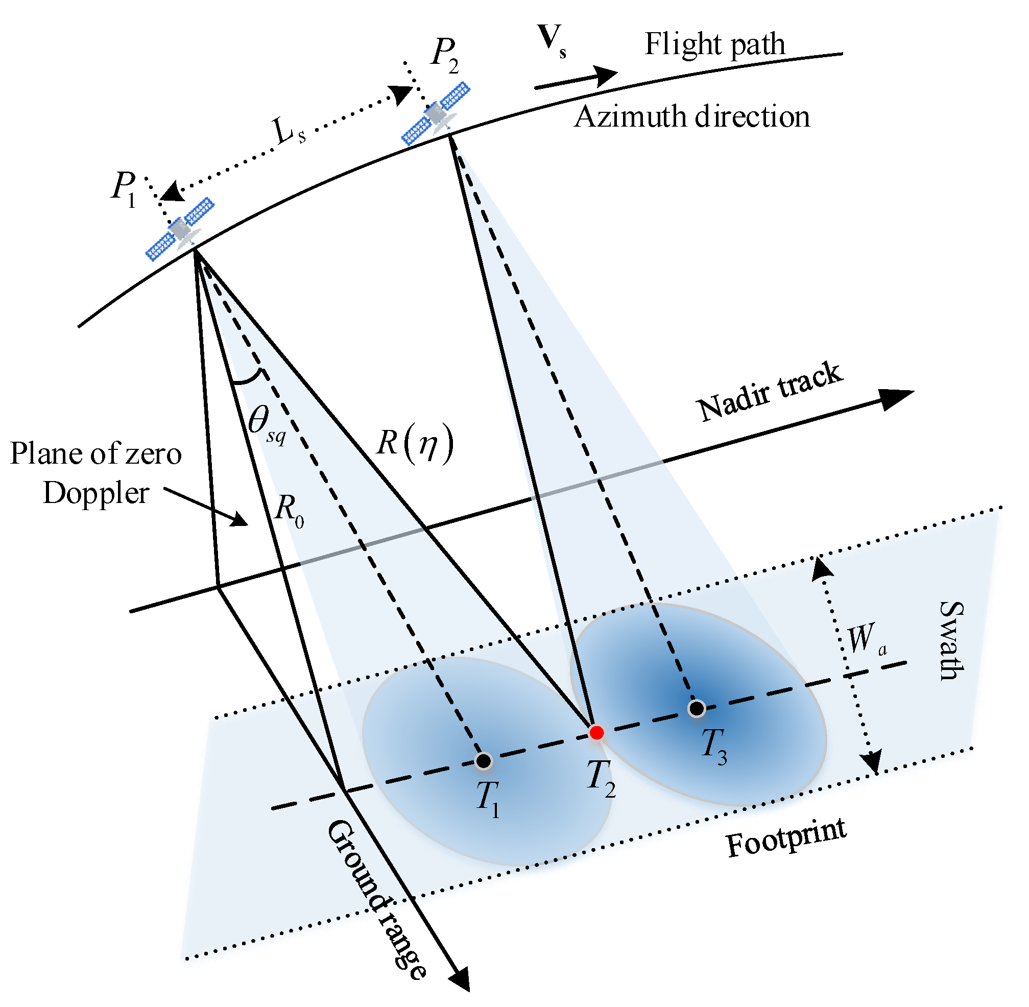
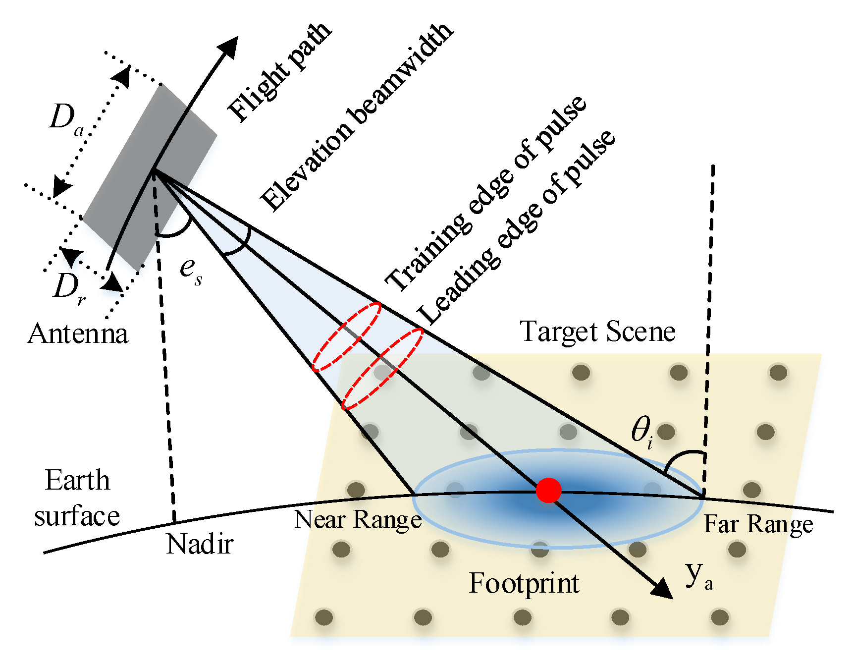
Figure 1 illustrates the geometric schematic diagram of SAR data acquisition. In this paper, we assume a monostatic radar system, in which the same antenna is used for both transmission and reception. As the radar moves along the flight path at a velocity of , the figure depicts a simplified geometric relationship between the radar’s position and the resulting beam footprint on the Earth’s surface in strip mode. The radar is located at point , as the target (marked by the red dot) enters the radar beam footprint, and leaves it at point . The length from to represents the synthetic aperture length of the target . Here, denotes the slant range between the radar system and the target. The slant range changes over time as the radar moves, until it reaches the minimum value known as the range of closest approach, . Furthermore, denotes the squint angle and describes the angle between the slant range vector and the zero Doppler plane.
In the range direction, the linear frequency modulation pulse emitted by the radar is
where represents the range time, is the carrier frequency of the radar, represents the frequency modulation (FM) rate of transmitted pulse chirp, and the pulse envelope can generally be approximated as a rectangle using , where is the pulse duration.
SAR receives the backscattered echoes after transmitting the LFM signal, and the baseband echo signal of a single point target after demodulation is as follows [26]:
where the complex constant A includes the amplitude of the backscatter coefficient of the point target and the phase change of the radar signal caused by scattering process. is the azimuth time, is the azimuth time when the beam center crosses, is the speed of light, is the radar carrier wavelength, is the two-way slant range of the received signal of the target at different azimuth times, and is the azimuth antenna pattern. The first exponential term in Equation (2) represents the phase history of the received signal, which effectively represents the distance change between the radar and the target.
When there are multiple point targets on the ground, the echo signal is the superposition of the echoes of each target, and Equation (2) can be used to obtain the echo signal under multiple point targets [18]:
where i and are the discrete azimuth time and the number of azimuth time sampling points, respectively. n is the distribution point in the scene scattering matrix, M is the number of point targets, and is the beam center crossing time of the nth target. is the round-trip distance between the radar and the nth target at azimuth time .
Equation (3) represents the demodulated baseband SAR signal received from all targets in the scene, with coefficient . It is the signal that is usually recorded or downlinked in a SAR system and referred to as the “raw data”, “SAR signal data”, or “SAR phase history” [26].
In the mathematical model of SAR echo signals, the key parameters are the solutions of and . The former is related to the position of the radar beam and the target, determining the azimuth time when the target is illuminated by the radar. The latter is related to the range model and determines the accuracy of range positioning and azimuth coherent accumulation. The range is the sum of transmission range and reception range, which are different in the “nonstop-and-go” configuration, similar to the range in the bistatic SAR [15].
For spaceborne SAR, calculating these two parameters is relatively complex because of factors such as the shape of the Earth, the orbit of the satellite, the spatial position of the radar, the random variation of satellite attitude errors, and the Earth’s rotation. In order to simulate SAR raw data that closely resemble actual data, it is crucial to establish a precise space geometry model between the satellite and the Earth to solve these parameters correctly.
3. Space Geometric Model of Spaceborne SAR
In spaceborne SAR, high azimuth resolution is achieved by accumulating coherent pulses in the azimuth direction through the motion of the satellite platform. The trajectory of the platform significantly impacts the SAR echo signal model, particularly the coherence of the azimuth pulse. Therefore, an accurate model of satellite–ground motion geometry is crucial for the signal model. This section mainly analyzes and introduces the spatial geometric relationship between the satellite, Earth, SAR antenna, and ground target from the perspective of the satellite–ground space geometry model.
3.1. Two-Body Orbit Model
The motion of a satellite around the Earth is primarily governed by the mutual gravitational attraction between the satellite and the Earth. The effects of other celestial bodies such as the Sun, Moon, and planets on the orbit of the satellite are typically insignificant and can be disregarded. As a result, a simplified two-body orbital model can be employed to describe the orbit of the satellite [2,27]. The satellite’s orbital period can be calculated using Kepler’s third law:
where the gravitational constant is .
After neglecting various perturbation forces, the satellite’s orbit can be calculated using Kepler’s three laws, and the satellite orbit equation [27] is
where a is the semi-major axis, f is the true anomaly, and e is the eccentricity.
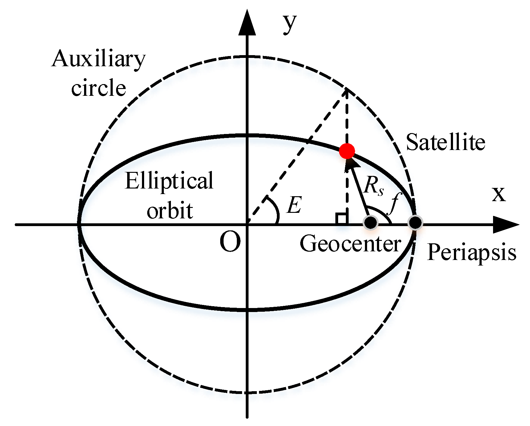
For SAR observation of the Earth, the satellite’s orbit is elliptical, with the eccentricity usually between 0 and 1. Figure 2 illustrates the elliptical orbit model with the Earth located at the focus of the elliptical orbit.
To solve the relationship between the position and time of the orbit, we introduce the eccentric anomaly E, which can be determined through constructing an auxiliary circle outside the ellipse. The eccentric anomaly can be calculated using Kepler’s equation [2,27]:
where the time of perigee passage is when the true anomaly f is 0.
The relationship between the true anomaly f and time can be established using Equations (6) and (7). The mean angular rate of the true anomaly, , and the mean anomaly, , change linearly with time. When the satellite completes one orbit, M changes from 0 to . Therefore, Kepler’s equation can be simplified as
However, Equation (8) cannot directly solve the analytical function relationship between position and time. An iterative method can be used to solve it, but its efficiency is low. In cases where the eccentricity , the Fourier series expansion can be used to approximate the analytical expression of the eccentric anomaly by ignoring the higher-order terms above [28]:
At any time on the orbit, the true anomaly f, the eccentric anomaly E, and the mean anomaly M have one-to-one correspondence.
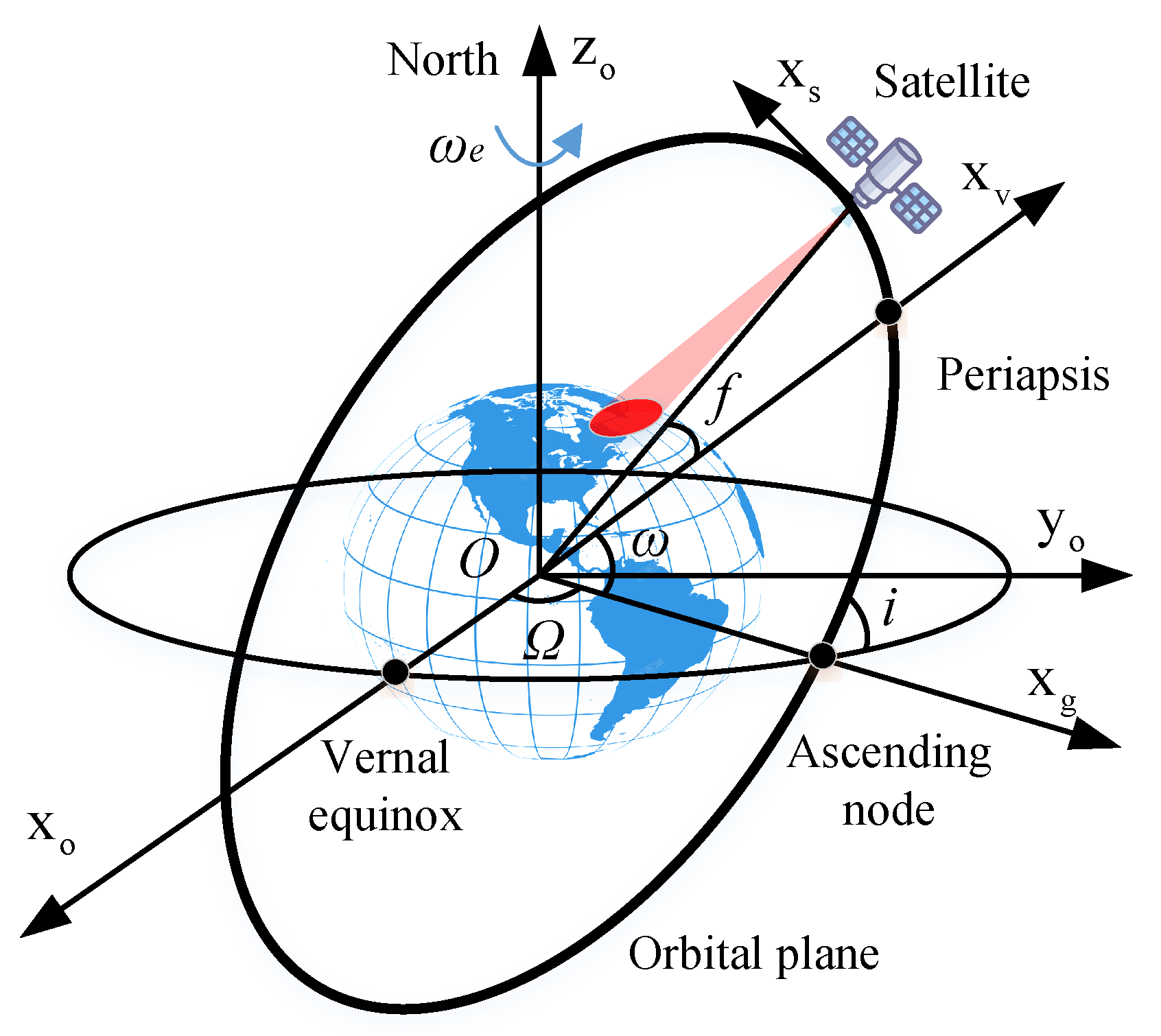
The position of the satellite on its elliptical orbit can be determined by the six orbital elements: semi-major axis a, eccentricity e, inclination i, right ascension of the ascending node , argument of perigee , and true anomaly f. The semi-major axis and eccentricity determine the size and shape of the satellite’s orbit. Meanwhile, the inclination, argument of perigee, and right ascension of ascending node (RANN) determine the orientation of the elliptical orbit in the orbital plane, while the true anomaly determines the instantaneous position of the satellite on the orbit [2].
The satellite’s orbital reference frame is established within the Earth-centered inertial coordinate system (ECI), as depicted in Figure 3, which illustrates the spatial configuration of the spaceborne SAR. The x-axis represents the direction towards the vernal equinox, while the xy-plane corresponds to the Earth’s equatorial plane. Furthermore, the z-axis is oriented towards the North Pole.
3.2. Earth Model
Since the Earth is not a perfect ellipsoid, the WGS-84 model is commonly used to describe the Earth’s shape and position in geodesy and satellite navigation. The WGS-84 model uses an ellipsoidal model with a semi-major axis of 6378.137 km and a semi-minor axis of 6356.752 km, which accurately describes the position on the Earth. The position of target on the Earth can be determined using
3.3. Spatial Coordinate Systems and Transformation Relationships
In order to model the operational process of a spaceborne SAR, determining the motion state of both the satellite and ground target is a critical step. However, this task can be challenging due to the intricacies involved in managing numerous coordinates and conversions between various coordinate systems [2]. Therefore, precise and efficient geometric modeling is essential.
The following eight coordinate systems are primarily involved in SAR geometric modeling: Earth-centered rotating coordinate system (ECR) , Earth-centered inertial coordinate system (ECI) , orbital plane coordinate system , satellite platform coordinate system , satellite body coordinate system , antenna coordinate system , satellite scene coordinate system , and ground coordinate system [2,27,28]. The specific definitions of these coordinate systems can be found in Table 1.
The transformation between various coordinate systems is essential in spaceborne SAR geometry modeling. The conversion of the space coordinate system mainly involves coordinate system translation and rotation.
Coordinate system translation occurs when two coordinate systems have different origins but have their coordinate axes pointing in the same direction. For example, given a point in space , after a coordinate system translation with a pointing vector of , the new coordinate of the point in the translated coordinate system becomes
Coordinate system rotation is the transformation of a coordinate system with the same origin through a rotation matrix . Similarly, suppose the coordinate of a point in space is , and it is rotated counterclockwise by angles of , , and around the x-axis, y-axis, and z-axis, respectively. The coordinates of the points in the new coordinate system are, respectively,
If the rotation is clockwise around the coordinate axis, the inverse of the rotation matrix can be used. Since the rotation matrix is an orthogonal matrix, its inverse matrix is equal to its transpose matrix.
The above eight coordinate systems in Table 1 can be interconverted through rotation and translation. Figure 4 shows the transformation relationships and transformation matrices between the coordinate systems. Note that the translation transformation is not included in the transformation matrix. The transformation from the orbital plane coordinate system to the satellite platform coordinate system requires translation along the satellite position vector, while the transformation from the satellite body coordinate system to the antenna coordinate system requires translation along the antenna position vector. Additionally, the transformation from the ground coordinate system to the ECR coordinate system requires translation along the scene center position vector [2,27,28].
The rotation matrix for transforming from the ECI coordinate system to the ECR coordinate system is
which involves a counterclockwise rotation around the z-axis by a Greenwich Mean Sidereal Time angle , where e is the angular velocity of the Earth’s rotation and is any reference time.
Similarly, the rotation matrix for converting from the ECI coordinate system to the orbital plane coordinate system is given by
where i is the inclination, is the RAAN, and is the argument of perigee.
To transform the orbital plane coordinate system to the satellite platform coordinate system , the rotation matrix is defined as
where is the track angle, which is the angle between the position vector and the orbit normal vector.
The rotation matrix for converting from the satellite platform coordinate system to the satellite body coordinate system is defined as
where , , and are the satellite’s pitch angle, roll angle, and yaw angle, respectively.
The rotation matrix for transforming from the satellite body coordinate system to the antenna coordinate system is defined as
where is the antenna’s off-nadir angle, with a positive value indicating left viewing and a negative value indicating right viewing.
To convert from the satellite scene coordinate system to the ground coordinate system , the rotation matrix is defined as
where represents the satellite heading angle, defined as the angle between the satellite’s flight direction and the North Pole, with the clockwise direction as positive.
Finally, the rotation matrix for converting from the ground coordinate system to the ECR coordinate system is defined as
where and are the geodetic longitude and latitude of the ground scene center, respectively.
These rotation matrices play a significant role in SAR geometric modeling for generating high-quality SAR raw data. Moreover, in the analysis and parameter solving of the spaceborne SAR geometry model, it is vital to select appropriate coordinate systems according to various scenes, which can effectively reduce the complexity of the analysis.
3.4. Solution of the State Vector of Space-Earth Motion
To simulate the SAR raw data and solve the imaging parameters of the spaceborne SAR, the motion state vector of the satellite and the target on the Earth during the synthetic aperture time must be used.
The solution for the satellite’s motion vector is more conveniently obtained in the orbital plane coordinate system . The true anomaly f and the orbital radius , both varying with time, can be calculated by Equation (5) and Equation (7), respectively. Then, the position vector and velocity vector of the satellite in are obtained as follows [2,28]:
When a satellite travels along an elliptical orbit, the beam of SAR scans over a larger area on the Earth, known as the beam’s footprint. The beam intersects the ellipsoidal surface of the Earth at a set of points, with each point being referred to as an “aiming point” of the beam. In SAR imaging, the imaging swath’s center is determined by the aiming points, which represent the intersection between the SAR beam’s centerline and the Earth’s surface.
Assuming that the aiming point of the beam in the antenna coordinate system has coordinates , where is the distance from the satellite to the aiming point, which is the parameter to be solved. Through the utilization of the two-body elliptical orbit model and coordinate system transformation, the coordinates of the aiming point can be converted into the ECR coordinate system . Thereafter, by substituting the coordinates of the aiming point within the into the smooth ellipsoidal Earth model, an analytical value can be determined [2,13]. Let the position vector of the antenna phase center in the satellite body coordinate system be ; then, the position vector of the aiming point in the antenna coordinate system [13] is
By solving Equation (10) with the obtained position vector , the value of should be the minimum of the two solutions. If the solution is a complex number, it indicates that the centerline of the beam has deviated from the Earth.
The motion vector of the target on the Earth is more convenient to solve in the ECR coordinate system . In SAR raw data simulation, the position of the target point is generally represented in the satellite scene coordinate system , whose origin is the scene center. To simulate the SAR imaging process and generate realistic raw data, it is necessary to determine the position of the scene center.
Typically, SAR systems will consider the aiming point of the beam at the imaging center time as the scene center, which is also the center of the imaging swath. This point serves as the reference point for the scene coordinate system. After obtaining the coordinates of the center in the ECR coordinate system by Equation (24), the coordinates of other targets in the scene can be transformed into using the transformation matrices and . The transformation relationship is
where is the position vector of other targets in the satellite scene coordinate system and is the position vector of the beam’s aiming point in the ECR coordinate system at the imaging center time.
In the ECR coordinate system , the position vector of all targets on the ground remains unchanged and their velocity vector is .
4. Spaceborne SAR Raw Data Simulation
Spaceborne SAR systems can operate in different modes, including stripmap mode, spotlight mode, sliding spotlight mode, scanning mode, etc. The main difference among these modes is the variation in beam control, while the echo models are fundamentally similar. This paper mainly focuses on the stripmap mode to introduce raw data simulation.
4.1. Accurate Range Model with “Nonstop-and-Go” Configuration
The “stop-and-go” assumption is the foundation of the SAR signal theoretical model, which assumes that the radar platform remains stationary during the transmission and reception of the backscattered echoes. Consequently, the echo delay is simplified as twice the slant range at the time of signal transmission. However, this assumption neglects the motion of the radar platform during signal transmission, propagation, and reception, resulting in two types of errors: one related to the slant range caused by the motion of the radar platform during transmission and reception, and the other relating to the slant range caused by the motion of the radar platform during signal transmission [7,29].
The first type of error can generally be ignored in SAR systems. For the second type of error, it can be ignored in airborne SAR and low-resolution spaceborne SAR; however, for high-resolution spaceborne SAR, medium-to-high orbit SAR, and geosynchronous orbit SAR, the error will seriously affect the focusing effect [30].
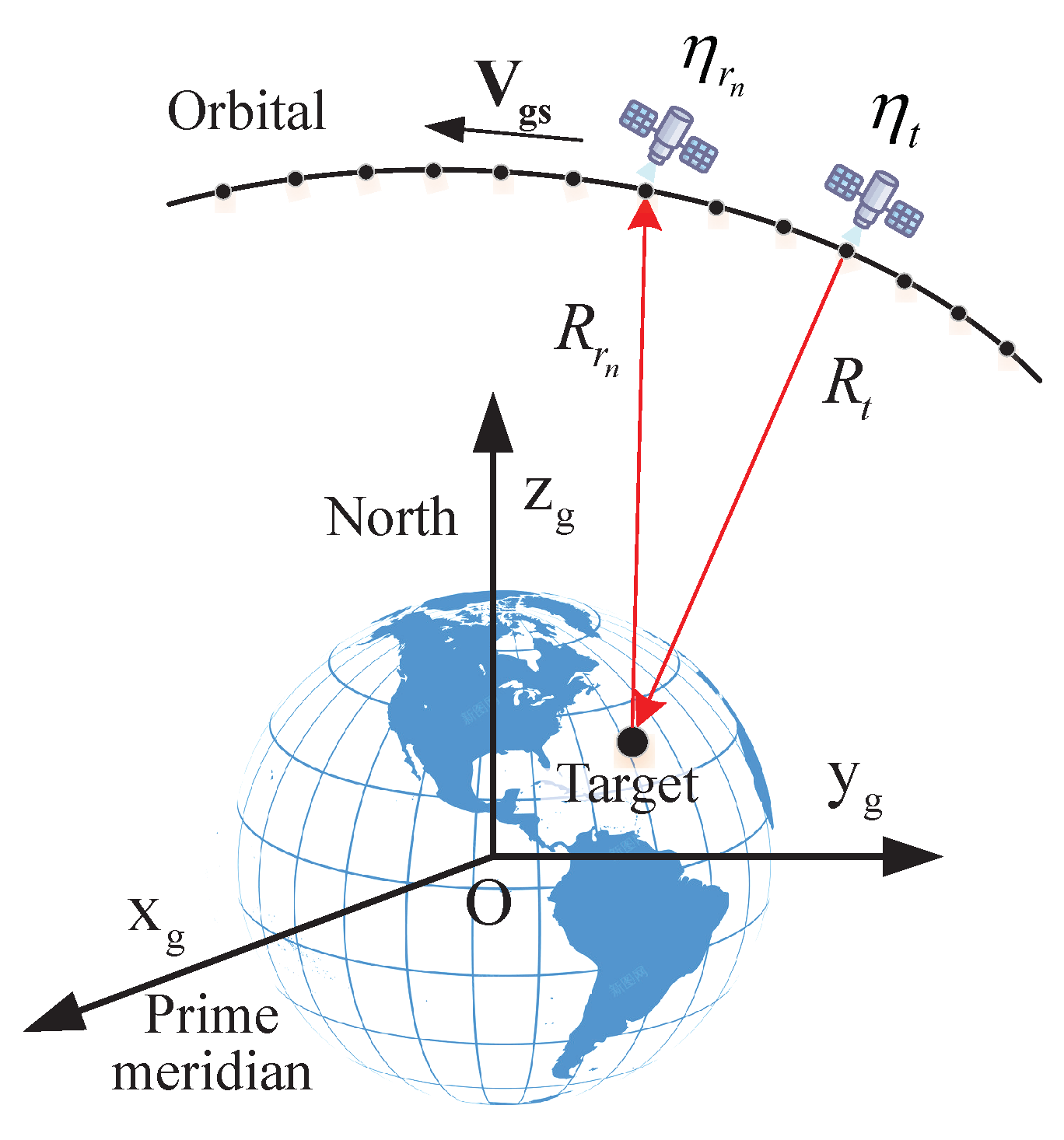
Therefore, in spaceborne SAR raw data simulation, it is necessary to establish a real motion model with the configuration of “nonstop-and-go” according to the geometric relationship between the satellite and the target, and calculate the true slant range of each scattering point. By choosing to analyze in the ECR coordinate system, the calculation complexity can be simplified. In this coordinate system, only the satellite is in motion, while the target is relatively stationary.
With the configuration of “nonstop-and-go”, the spatial geometry between the satellite and the target can be shown as in Figure 5. The radar travels along the orbit at a velocity of , constantly emitting electromagnetic waves and receiving echoes from the target. Assuming that the radar emits electromagnetic waves at time , the distance between the target and the radar at this moment is . When the electromagnetic wave reaches the target and reflects back to be received by the radar, the radar has moved to time , corresponding to a distance of . In the configuration of “nonstop-and-go”, and are different.
The actual slant range of the echo signal consists of two parts: the transmission range and the reception range. At a certain azimuth moment, the radar first sends a pulse signal to the target and the transmission range can be obtained by calculating the distance between the satellite and the target at this time. Then, while the radar platform is moving, it waits for the echo signal reflected by the target. However, the reception time cannot be directly solved because of the relative motion between the two. This means that the position of the satellite cannot be obtained and, therefore, the reception range cannot be determined. Since there is no analytic solution for the echo delay calculation, an iterative method is needed to solve it [31]. The process of the iterative solution is as follows:
- At a certain azimuth moment , the radar transmits a pulse signal towards the target and calculates the position of the satellite and the transmission range ;
- By iterating to solve the azimuth moment of receiving the echo signal from the target , let , and set its initial value to ;
- After n iterations, calculate the position of the satellite when the echo signal is received at the azimuth time . Then, calculate the reception range of the echo signal at this time;
- Calculate the iteration error . If it is less than the preset accuracy, the iteration is completed, and the final reception range of the target echo signal is . Otherwise, set , , and continue to iterate in step 3 until the required accuracy is met. Generally, the error tolerance can be set to one-quarter of the wavelength to meet the precision requirements.
The slant range obtained by iterative solution has high accuracy and eliminates the slant range error caused by the traditional “stop-and-go” assumption. It can be used for modeling the distance of any spaceborne SAR at any orbit altitude.
4.2. Determination of Beam Illumination Area
The positions of target objects in simulated terrain scenes are located in the satellite scene coordinate system, with the scene center as the origin. During SAR raw data simulation, the scene plane coordinate system is assumed to align with the local horizontal plane of the ground point where the scene center is located. As the satellite moves, the SAR beam scans the ground and only those scattering units within the beam illumination area are considered. The schematic diagram of the target scene area illuminated by spaceborne SAR is shown in Figure 6.
As the radar beam moves, the scattering units of a scene reflect radar echoes that undergo continuous changes. Therefore, it is important to determine whether each target point within the scene falls within the beam illumination area at each moment in azimuth. When the length of the antenna in both the azimuth and elevation directions are equal, the angle formed between the target and the radar line-of-sight vector can be compared with the beam width during each azimuth moment to determine whether a particular target falls within the beam illumination range [9].
However, in practical applications of SAR, such as strip mode, the shorter the length of the elevation antenna, the wider the beam illumination area, and the shorter the length of the azimuth antenna, the higher the azimuth resolution. Furthermore, due to constraints on the antenna’s minimum area, weight, and volume, the azimuth dimension of spaceborne SAR antennas is generally larger than that of the elevation dimension. Therefore, the above judgment method may not be applicable.
This paper proposes an effective method for judging the elliptical beam illumination area when the widths of the antenna’s azimuth and elevation beams differ. The specific steps are as follows:
First, the target’s position vector in the antenna coordinate system is calculated for each azimuth moment using
where represents the target’s position vector in the . Equation (26) mainly completes the transformation of the target position vector from the ECR coordinate system to the antenna coordinate system . More detailed information on coordinate transformation can be found in Section 3.3. Since the y-axis of the antenna coordinate system coincides with the centerline of the beam, its coordinate value represents the distance from the target to the center of the antenna.
Then, the projection of the 3 dB beamwidth [26] of the radar on the azimuth and elevation directions is calculated separately for the corresponding distance :
where and correspond to the lengths of the antenna’s azimuth and elevation directions, respectively, and and correspond to the widths of the beam coverage area in the azimuth and elevation directions, respectively, which correspond to the major and minor axes of elliptical beam cross section.
Finally, whether the target will reflect echo signals at the current azimuth moment is determined by judging whether the target is within the elliptical beam region determined by and . The judgment criteria are as follows:
With this method, the elliptical beam illumination range can be determined accurately even when the antenna’s azimuth and elevation widths differ.
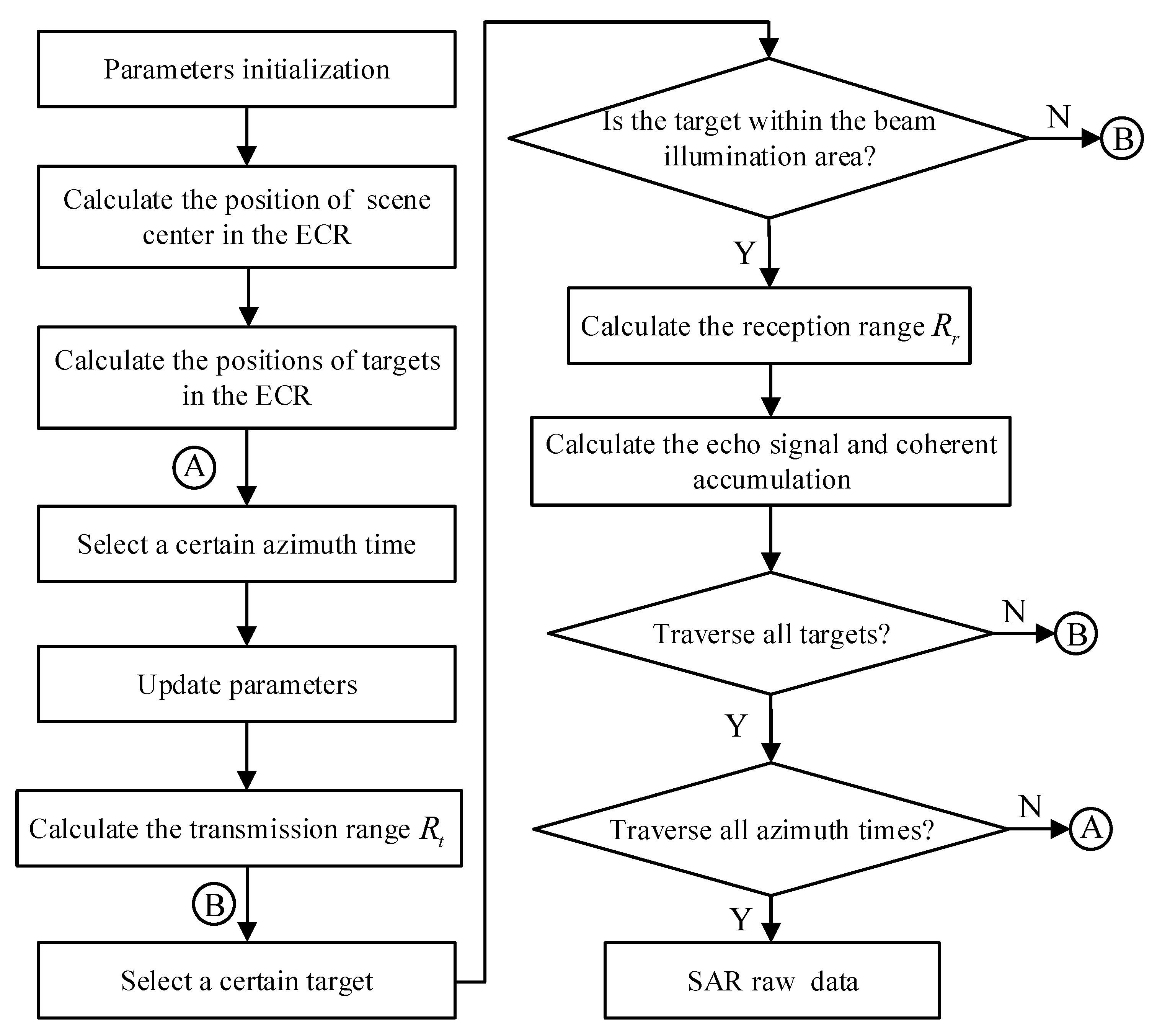
4.3. Raw Data Simulation Based on Time-Domain Method
Time-domain raw data simulation is considered the most classical and precise method for generating SAR raw data. The process involves the transmission of LFM pulse signals during the motion of the radar platform, followed by the reception of echoes from targets located within the beam illumination area. The raw echo data are obtained through recursive coherent summing [13]. In this paper, we present the specific steps for conducting time-domain raw data simulation:
- Initialize the system parameters, including satellite orbit and attitude parameters, Earth model parameters, SAR working parameters, simulation scene parameters, coordinate transformation matrices, etc.
- Calculate the position coordinates of the scene center in the ECR coordinate system based on the space geometry model of the spaceborne SAR and calculate the coordinates of other targets in the scene based on the scene coordinate transformation.
- Compute the orbital parameters, coordinate transformation matrices, and satellite position at a certain azimuth moment.
- Transform the coordinates of each target in the scene to the antenna coordinate system and judge whether they are within the beam illumination area according to the theory introduced in Section 4.2.
- Compute the transmission distance and reception range for each target within the beam illumination area, sum them up as the propagation distance of the signal, and calculate the target’s echo signal.
- Coherently accumulate the echoes of all targets at this azimuth moment, calculate the next azimuth moment, and continue until all azimuth moments have been traversed.
- Finally, simulated echo data of the targets are obtained; details of the echo simulation flow are illustrated in the Figure 7.
In general, this method of raw data simulation provides high-precision spaceborne SAR data that can be used for a variety of working modes and even for SAR at a higher orbit altitude.
5. Simulation Results and Analysis
In this section, the raw data of SAR in strip mode based on a low earth orbit (LEO) satellite are generated and analyzed through focusing imaging. Firstly, the key parameter analysis results of satellite spatial geometry modeling based on the two-body orbit model are presented. Then, point target scene simulation analysis is carried out by setting system simulation input parameters as shown in Table 2.
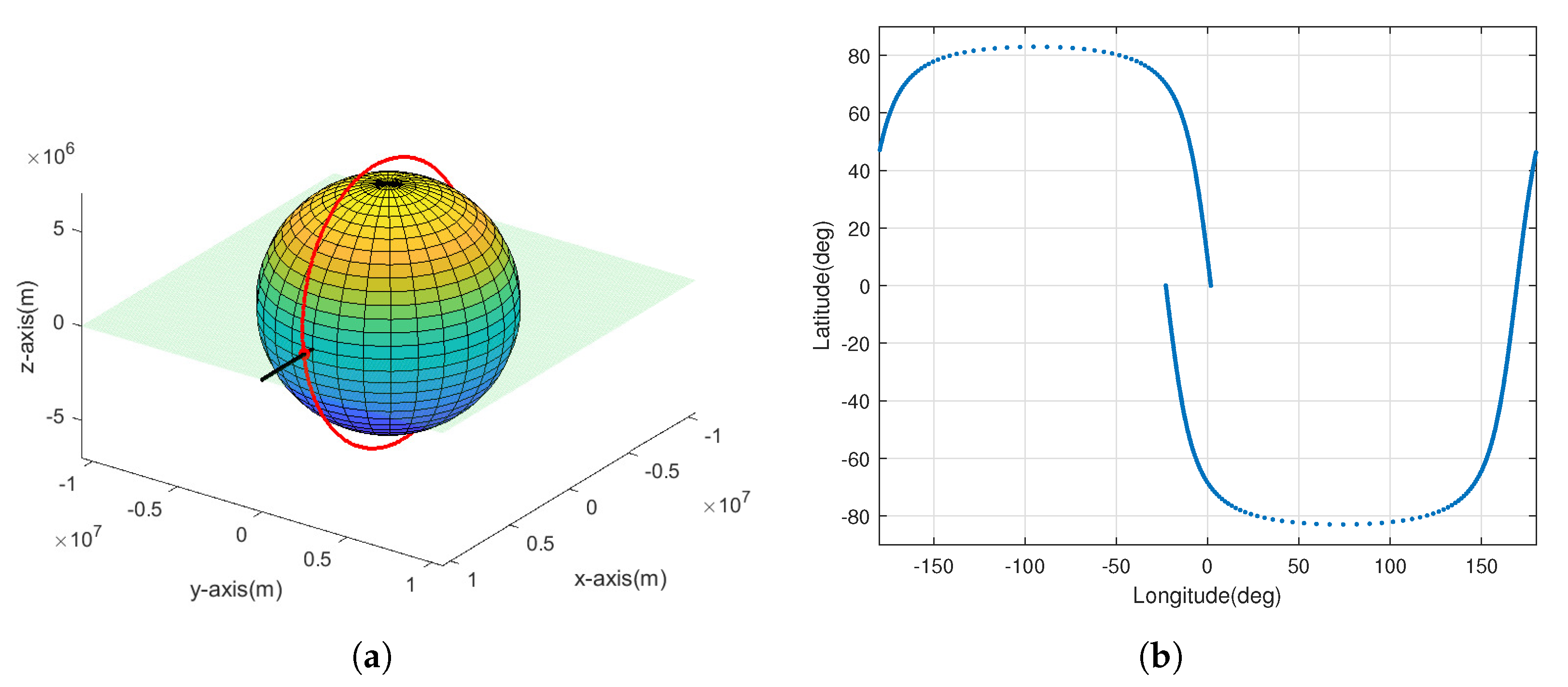
5.1. Simulation of Satellite Key Parameters
According to the two-body orbit model introduced in Section 3.1, the satellite’s motion trajectory for one orbit period was simulated first. The satellite’s motion trajectory in the ECI coordinate system is shown in Figure 8a, where the red curve represents the satellite’s motion trajectory, the black line represents the direction of the vernal equinox, and the green plane represents the equatorial plane. It can be seen that due to the small eccentricity of the elliptical orbit, the orbit is approximately circular. As shown in Figure 8b, the shape of the nadir track is influenced by various factors, including satellite orbit height, orbit inclination, and the Earth’s rotation. The discontinuities presented in the figure are caused by the Earth’s rotation. While the satellite is moving, the Earth is also rotating around its axis and the interaction between these two movements affects the shape of the nadir track, resulting in the discontinuities observed in the middle part of the figure.
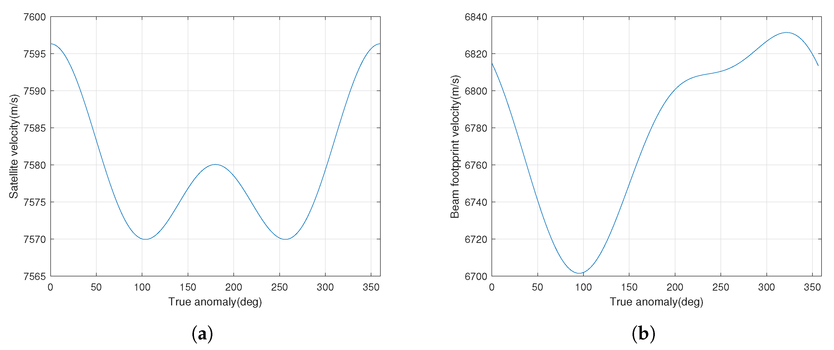
For the spaceborne SAR, the geometric relationship is more complex than that of the airborne SAR since both the orbit and the Earth’s surface are curved, and the Earth rotates independently of the satellite’s orbit. The platform velocity of the satellite and the ground forward speed of the beam coverage area differ significantly and vary with the orbit position. The variations of and with true anomaly angle f within one orbit period are shown in Figure 9a and Figure 9b, respectively. It can be seen that both velocities change differently at different positions within the orbit, which means that they are range-variant in the azimuth direction.
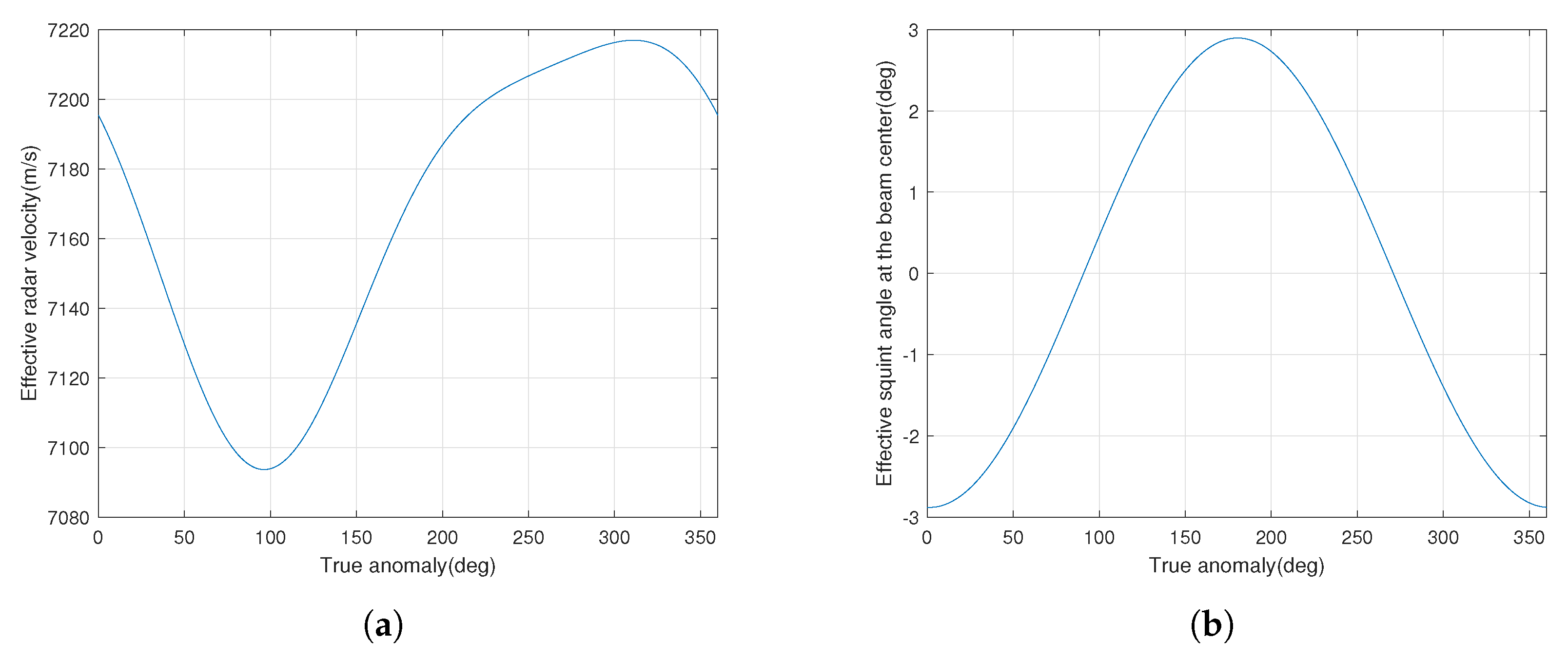
In the case of the airborne SAR, because the platform velocity and the ground speed along the beam coverage area are consistent, and the flight path can be equivalent to a straight line, the range equation in the SAR model is a hyperbolic model. However, for the spaceborne SAR, due to the difference in spatial geometry, it is generally necessary to assume that the orbit is locally linear and the Earth is locally flat without rotation to make the range equation equivalent to the hyperbolic model. To achieve this, the effective radar velocity and the effective squint angle at the scene center moment are introduced. We provide an investigation of the variations of and with the true anomaly within one orbit, which are presented in Figure 10a and Figure 10b, respectively.
The effective radar velocity and the effective squint angle are analyzed based on the accurate geometric model of the spaceborne SAR and obtained by solving the Doppler parameters. It can be seen that even in the case of broadside, the squint angle of the spaceborne SAR is not zero due to the Earth’s curvature and rotation. The maximum squint angle occurs near the equator while the minimum occurs at the poles. It is evident that simulating raw data for spaceborne SAR is more complex than for airborne SAR. Establishing an accurate space geometry model for spaceborne SAR is crucial to develop an accurate range model.
5.2. Simulation of Slant Range with “Nonstop-and-Go” Configuration
Simulating spaceborne SAR presents a challenge due to the significant signal propagation time and high satellite speed. Therefore, we perform simulations using both “stop-and-go” assumption and “nonstop-and-go” configuration with the geometric model and iterative solution method introduced in Section 4.1.
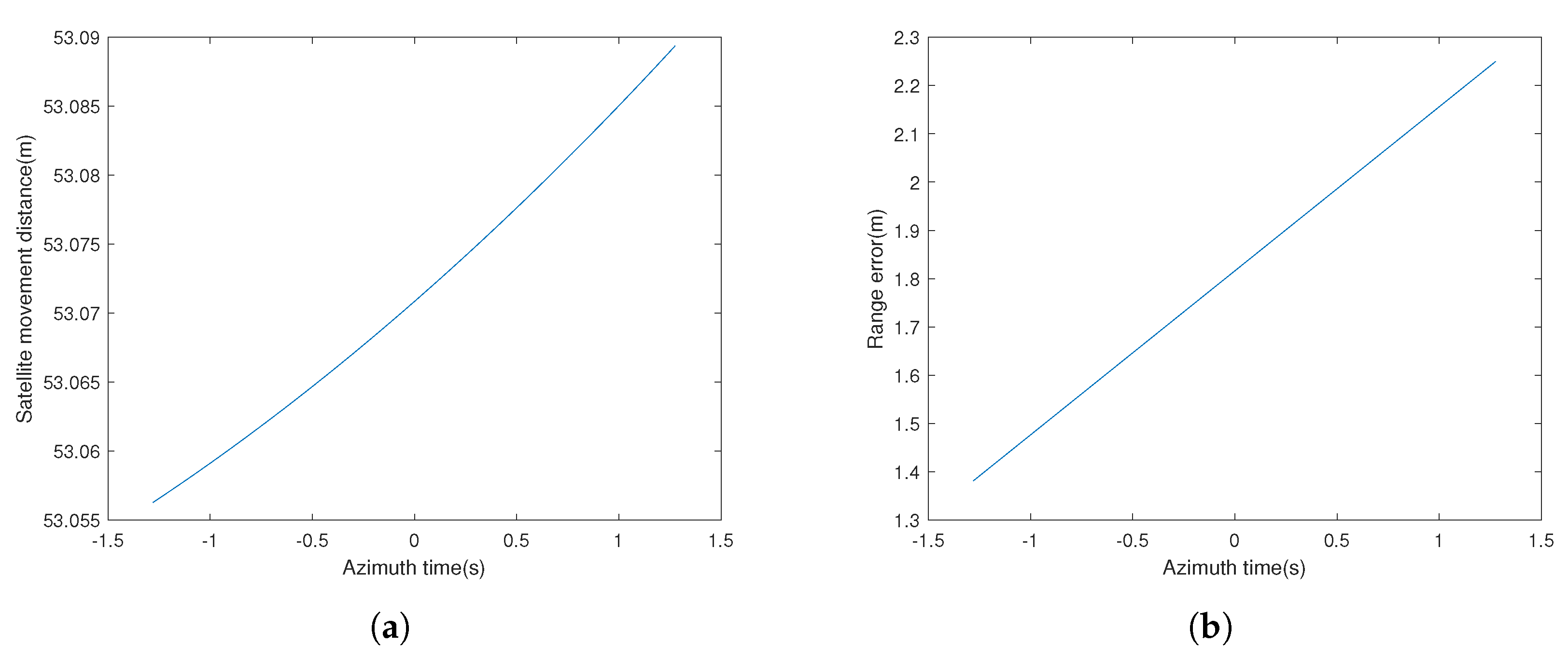
The distance that the satellite platform moves during signal transmission, propagation, and reception is shown in Figure 11a. It can be seen that if we adopt the “stop-and-go” assumption and assume that the position of the radar platform during the signal transmission, propagation, and reception is stationary, a position deviation of more than 50 meters will occur. The slant range errors with both “stop-and-go” assumption and “nonstop-and-go” configuration are shown in Figure 11b. The results highlight that the slant range error produced by the “stop-and-go” assumption exceeds one-quarter of the signal wavelength, leading to considerable errors in the raw data simulation of spaceborne SAR.
The findings emphasize the vital role of considering the motion of the satellite during signal transmission when conducting simulations for spaceborne SAR. Establishing a precise space geometry model is crucial in developing an accurate range model for simulating raw data in spaceborne SAR. These insights are essential for researchers working towards developing reliable SAR models, highlighting the need to account for the effects of satellite motion in simulations.
5.3. Raw Data Simulation and Imaging Analysis
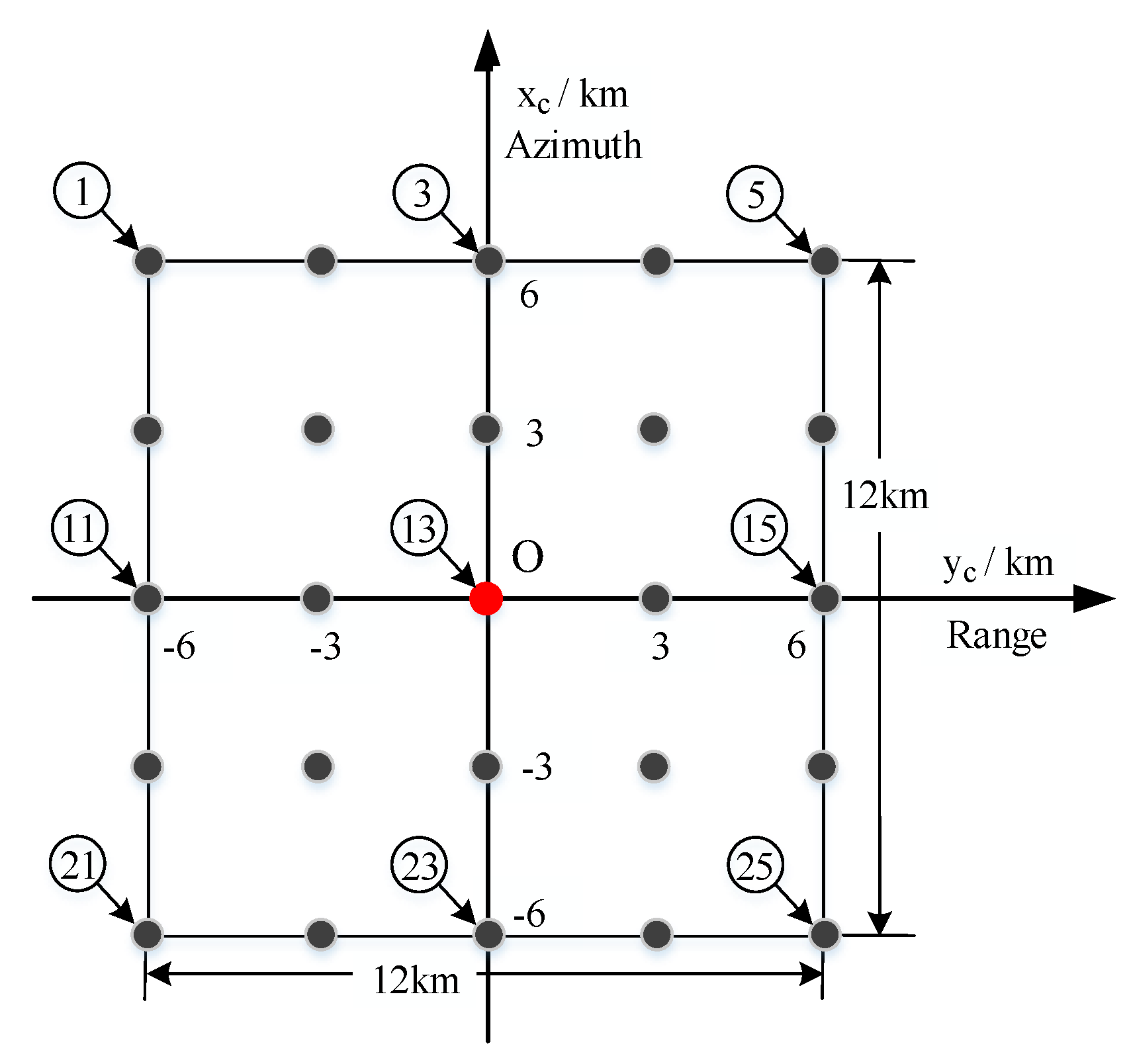
In this subsection, the time-domain raw data simulation method is used to simulate and generate point target raw data, which are then focused on and analyzed. The position distribution of the point targets in the scene is given in the satellite scene coordinate system, as shown in Figure 12. There were 25 targets in total, and target 13 was located at the center of the scene. The vertical and horizontal intervals between each target were both 3 km.
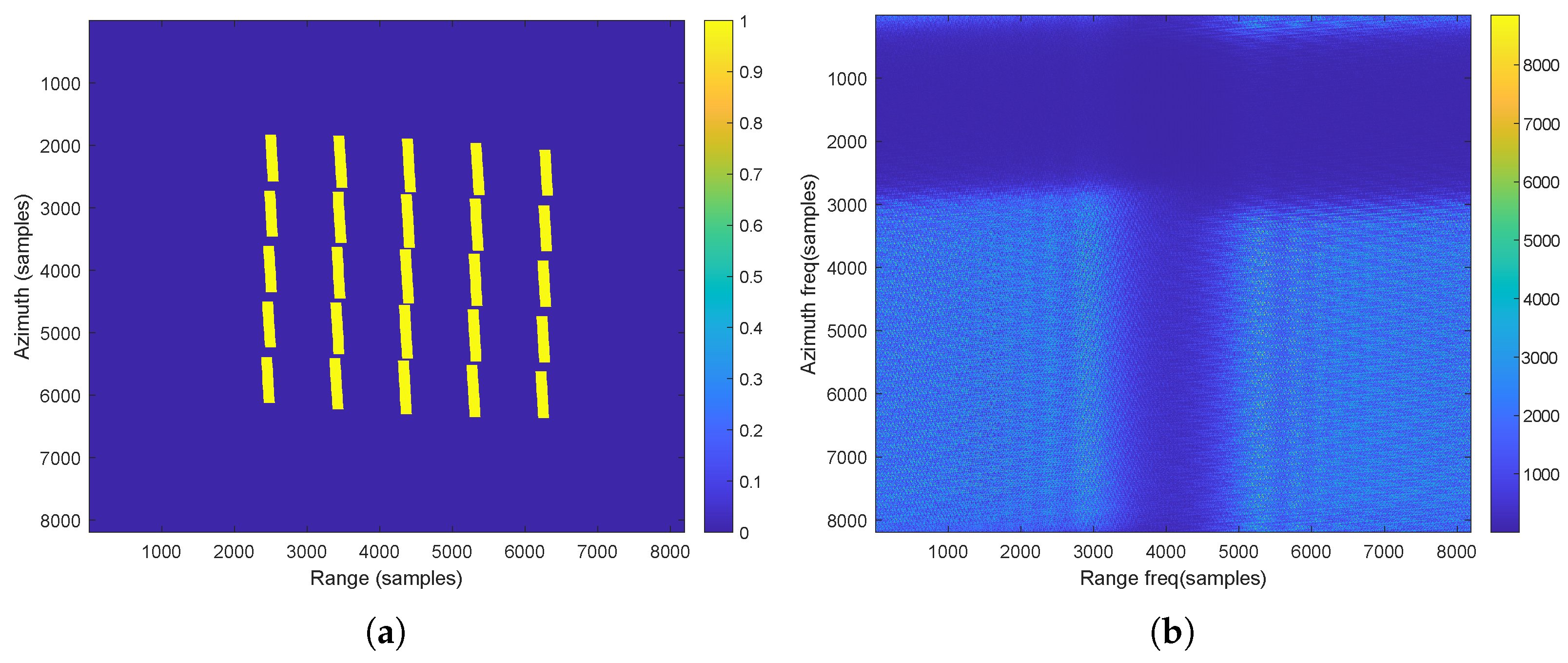
Figure 13a and Figure 13b, respectively, show the amplitude values of the two-dimensional time-domain and frequency-domain of the acquired raw data from the simulated point target scene. These figures were obtained by setting parameters according to Table 2.
In Figure 13a, it can be seen that the targets at the edge of the scene have shorter azimuth echo durations relative to the central target due to the antenna’s elliptical beam. This is because the targets deviated from the beam center are illuminated for a shorter time, resulting in a shorter synthetic aperture length of the target. The simulation of a target scene was performed with the assumption that all targets have identical reflectivity, and factors such as propagation attenuation were not considered. Therefore, the amplitude of the echo signal (yellow area) at each azimuthal moment for all targets is the same. In Figure 13b, there are gaps (dark blue areas) in both the azimuth and range directions in the two-dimensional frequency domain due to oversampling. The squint angle causes the azimuth spectrum gap to be not in the middle and there is a frequency tilt.
The chirp scaling algorithm (CSA) [26,32] was employed to process the raw data, which is an accurate imaging algorithm with high precision and can meet the imaging requirements of SAR systems with large squint angle. CSA utilizes the LFM characteristics of the transmitted signal for accurate range cell migration correction (RCMC), completely avoiding interpolation operation. Imaging can be achieved through complex multiplication, fast Fourier transform (FFT), and inverse FFT (IFFT). Furthermore, the CSA algorithm can maintain good phase accuracy.
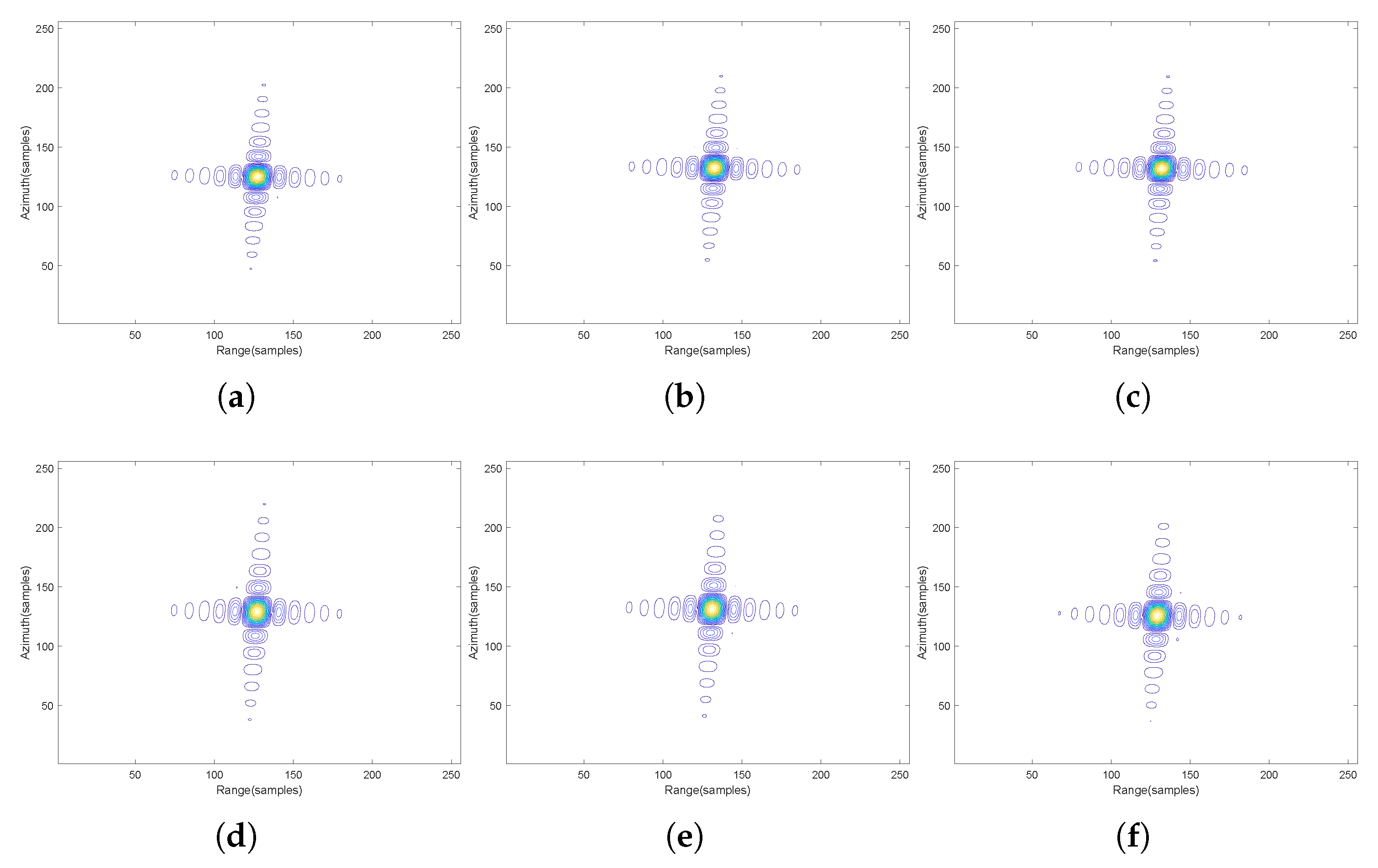
The contour images of typical targets 3, 5, 13, 15, 23, and 25 are shown in Figure 14. Each target was sliced into a image with peak value as the center and upsampled by 8 times.
From Figure 14, it can be seen that each target had symmetrical sidelobes, indicating that the targets were well focused and the sidelobe tilt was caused by non-zero squint angle.
With the same simulation parameters, we conducted a comparative study on the imaging positions of selected targets under different models that simulate raw data of the LEO SAR. Specifically, we compared the traditional hyperbolic range model, which assumes constant-speed linear motion of the radar platform and is based on the “stop-and-go” assumption (the simulation parameters for the equivalent radar velocity and equivalent squint angle are selected at the azimuth center moment in Section 5.1), with a curved orbit model, which considers the Earth’s elliptical shape and rotation, and with the accurate range model with “nonstop-and-go” configuration presented in this paper. Table 3 provides the imaging positions of selected targets under the above models.
From Table 3, it is evident that the imaging position of the target is more consistent with the theoretical value for the traditional hyperbolic range model. However, the other two models showed deviations from the range direction (except for the scene center) and azimuth direction due to the inclusion of additional factors such as curved orbits, the elliptical shape of the Earth, and the Earth’s rotation. These deviations often require subsequent geocoding processing [1]. Because the synthetic aperture time is short and the imaging resolution is relatively low, the “stop-and-go” assumption-based model only causes offset variation in the azimuth direction; there are seven sample points with azimuth offset observed from Table 3.
To more accurately measure the imaging quality of the raw data, the quality parameters of the point targets were measured, including impulse response width (IRW), peak sidelobe ratio (PSLR), and integrated sidelobe ratio (ISLR) [26]. Firstly, the point target imaging result was rotated so that most of the sidelobes aligned with the horizontal or vertical axis; then, the range and azimuth envelopes at the target peak were extracted separately; finally, the three quality parameters were measured. No weighting processing was used in the azimuth and range directions during imaging. Based on the processed raw data generated by the three models presented in Table 3, the quality parameters of the selected target points were measured and the results are shown in Table 4.
The IRW refers to the 3 dB main lobe width of the impulse response, which is also known as the image resolution in SAR processing. The theoretical range resolution is [26]. It can be observed from Table 4 that the results obtained from all three models are generally consistent with the theoretical values. For the traditional hyperbolic model, the theoretical azimuth resolution is . However, for the model based on elliptical orbit, the azimuth resolution should be calculated as [26]. Due to the antenna elliptical beam, the time for far targets from the beam center to be illuminated is relatively shortened, resulting in a shorter synthetic aperture length, thus reducing the azimuth resolution. Therefore, targets 5, 15, and 25 have lower azimuth resolutions than those of targets 3, 13, and 23.
The PSLR determines the resolution of the SAR and the ISLR is related to the image contrast. Since no windowing function was used during imaging, the PSLR and ISLR of the sinc function were both ideal values, which were −13.26 dB and −10.16 dB, respectively. Due to the relatively low resolution, CSA can be used to perform good focus processing. As shown in Table 4, the measurement results of the three models for the targets are generally close to the theoretical values, indicating that the point targets are well focused and the precision of the raw data simulation.
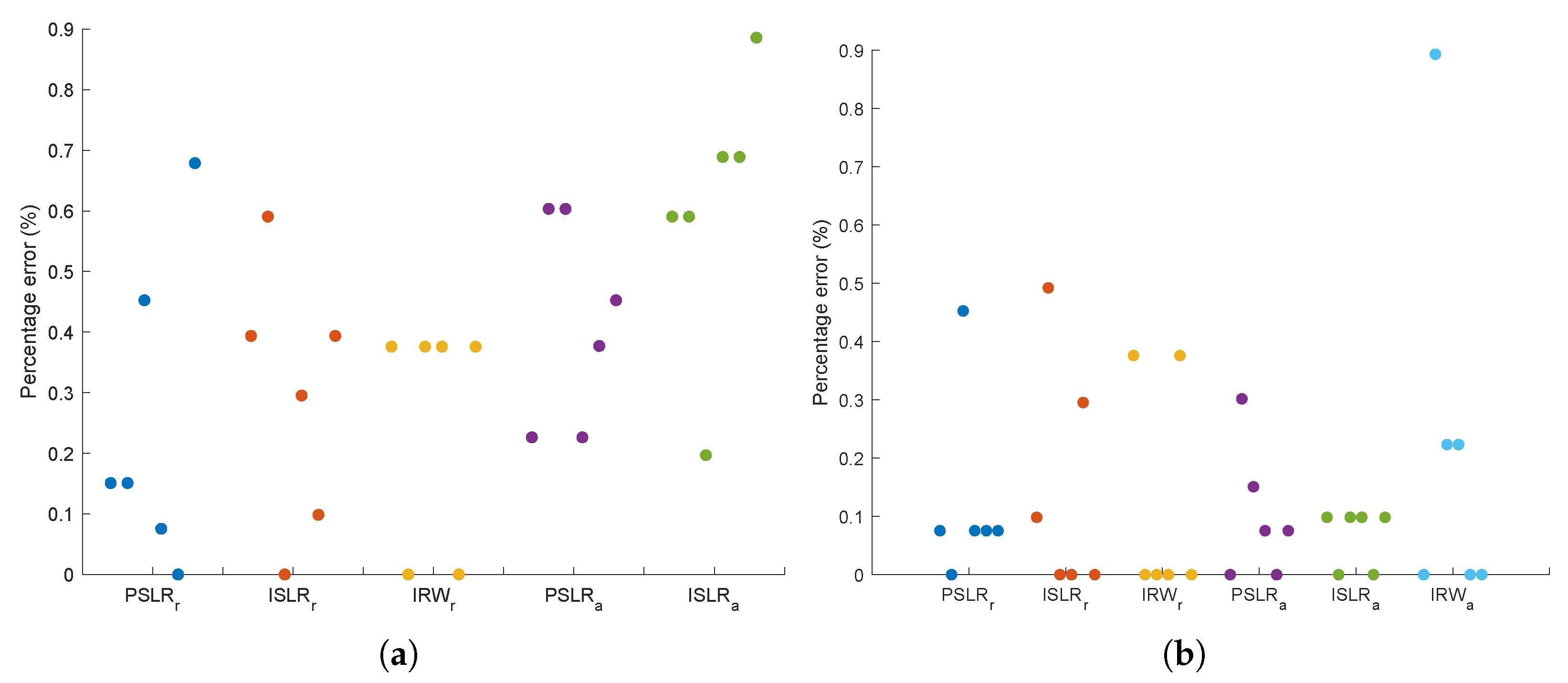
The point target imaging quality parameters obtained from the raw data using our proposed accurate model were compared with those obtained from two commonly used models, namely, the hyperbolic range model and the “stop-and-go” assumption-based model. The percentage errors for each parameter are presented in Figure 15a and Figure 15b, where the subscripts ‘r’ and ‘a’ indicate range and azimuth parameters, respectively. It is worth noting that the azimuth resolution of the traditional hyperbolic range model is not compared in Figure 15a, as its formula is not applicable to spaceborne SAR. The results demonstrate that our proposed method has an imaging error of less than 1% compared to the other two ideal models, indicating its high accuracy. Moreover, our model performs better in representing realistic spaceborne SAR scenarios than the other two models, thus showing its superiority.
After analyzing the imaging processing of SAR raw data generated by three models, we concluded that utilizing a precise slant range model based on the space geometry of satellite-borne SAR, as implemented in this study, produces raw data that more closely resembles real SAR data than the other two models. Without considering the effects of atmospheric and ionospheric influences as well as perturbations caused by other celestial bodies, our model remains accurate and can serve as a reference benchmark for other methods. Currently limited to simulating strip mode with low resolution, future simulations using beam mode can be conducted to validate high-resolution and ultra-high-resolution imaging algorithms.
6. Conclusions
After identifying the many approximation problems in the existing simulation of raw data for spaceborne SAR, this paper has successfully proposed a more accurate method for simulating raw data. By analyzing the motion state vectors of the satellite and ground targets, we were able to model the space geometry of spaceborne SAR. Based on the two-body orbit model and the Earth ellipsoid model, we established a precise slant range model with a “nonstop-and-go” configuration and determined the target illumination area under the elliptical beam through spatial coordinate transformation. The raw data of the LEO SAR with strip mode were accurately simulated using the time-domain simulation method, and the data were imaged processed using the CSA. To evaluate the accuracy of the SAR raw data simulation method using our proposed accurate range model, we compared its imaging results with raw data generated by the hyperbolic range model and the curved orbit model based on the “stop-and-go” assumption. By analyzing the point target quality parameters, we found that the errors in our range model were within 1% when compared with the other two ideal models. Our proposed model demonstrated higher effectiveness in simulating SAR raw data, yielding simulated data that more closely approximates real SAR data than the other models. Furthermore, this method can be used to simulate raw data with other modes of SAR by using antenna beam control. It is also universal for spaceborne SAR raw data simulation at higher orbits. However, it is important to note that the influence of atmospheric transmission delay and dispersion caused by the ionosphere on the echo signals must be considered in future work. Additionally, as the number of targets in the simulation scene increases, improving the simulation speed while ensuring accuracy will be a challenging problem. Overall, this paper has significantly improved the accuracy of raw data simulation for spaceborne SAR and provides a valuable contribution to the development of remote sensing technology.
Author Contributions
Conceptualization, H.L. and J.A.; methodology, H.L.; software, H.L.; validation, H.L. and J.A.; formal analysis, H.L. and X.J.; investigation, H.L.; resources, H.L.; writing—original draft preparation, H.L. and M.L.; writing—review and editing, H.L., J.A., X.J., and M.L.; visualization, H.L. and M.L.; supervision, J.A. and X.J.; project administration, J.A. and X.J. All authors have read and agreed to the published version of the manuscript.
Funding
This research was supported by the National Key R&D Program of China under grant 2022YFF0503900 and Teaching Reform and Innovation Projects of Changzhi University under grant JC202105.
Institutional Review Board Statement
Not applicable.
Informed Consent Statement
Not applicable.
Data Availability Statement
The study did not report any data.
Conflicts of Interest
The authors declare no conflict of interest.
Abbreviations
The following abbreviations are used in this manuscript:
| CSA | chirp scaling algorithm |
| ECI | ECI (coordinate system) |
| ECR | ECR (coordinate system) |
| FFT | fast Fourier transform |
| FM | frequency modulation |
| IFFT | inverse FFT |
| IRW | impulse response width (resolution) |
| ISLR | integrated sidelobe ratio |
| LEO | low earth orbit |
| LFM | linear frequency modulation |
| PRF | pulse repetition frequency |
| PSLR | peak sidelobe ratio (ratio to main lobe) |
| RAAN | right ascension of the ascending node |
| RCMC | range cell migration correction |
| SAR | synthetic aperture radar |
| WGS-84 | World Geodetic System defined in 1984 |
| WSS | wrapped staring spotlight |
References
- Curlander, J.C.; Mcdonough, R.N. Synthetic Aperture Radar: Systems and Signal Processing; John Wiley & Sons: Hoboken, NJ, USA, 1991. [Google Scholar]
- Deng, Y. High-Resolution Wide-Swath SAR Imaging Technology for Spaceborne Platforms; Science Press: Beijing, China, 2020. [Google Scholar]
- Reigber, A.; Scheiber, R.; Jaeger, M.; Prats-Iraola, P.; Hajnsek, I.; Jagdhuber, T.; Papathanassiou, K.P.; Nannini, M.; Aguilera, E.; Baumgartner, S.; et al. Very-High-Resolution Airborne Synthetic Aperture Radar Imaging: Signal Processing and Applications. Proc. IEEE 2013, 101, 759–783. [Google Scholar] [CrossRef]
- Moreira, A.; Prats-Iraola, P.; Younis, M.; Krieger, G.; Hajnsek, I.; Papathanassiou, K.P. A Tutorial on Synthetic Aperture Radar. IEEE Geosci. Remote Sens. Mag. 2013, 1, 6–43. [Google Scholar] [CrossRef]
- Chen, J.; Yang, W.; Wang, P.; Zeng, H.; Men, Z.; Li, C. Review of Novel Azimuthal Multi-Angle Observation Spaceborne SAR Technique. J. Radars 2020, 9, 205–220. [Google Scholar]
- Bayir, I. A Glimpse to Future Commercial Spy Satellite Systems. In Proceedings of the 2009 4th International Conference on Recent Advances in Space Technologies, Istanbul, Turkey, 11–13 June 2009; pp. 370–375. [Google Scholar] [CrossRef]
- Prats-Iraola, P.; Scheiber, R.; Rodriguez-Cassola, M.; Mittermayer, J.; Wollstadt, S.; De Zan, F.; Brautigam, B.; Schwerdt, M.; Reigber, A.; Moreira, A. On the Processing of Very High Resolution Spaceborne SAR Data. IEEE Trans. Geosci. Remote Sens. 2014, 52, 6003–6016. [Google Scholar] [CrossRef]
- Mittermayer, J.; Kraus, T.; López-Dekker, P.; Prats-Iraola, P.; Krieger, G.; Moreira, A. Wrapped Staring Spotlight SAR. IEEE Trans. Geosci. Remote Sens. 2016, 54, 5745–5764. [Google Scholar] [CrossRef]
- Chen, Z.; Zeng, Z.; Huang, Y.; Wan, J.; Tan, X. SAR Raw Data Simulation for Fluctuant Terrain: A New Shadow Judgment Method and Simulation Result Evaluation Framework. IEEE Trans. Geosci. Remote Sens. 2022, 60, 1–18. [Google Scholar] [CrossRef]
- Kim, S.; Ka, M.H. SAR Raw Data Simulation for Multiple-Input Multiple-Output Video Synthetic Aperture Radar Using Beat Frequency Division Frequency Modulated Continuous Wave. Microw. Opt. Technol. Lett. 2019, 61, 1411–1418. [Google Scholar] [CrossRef]
- Lee, H.; Kim, K.W. An Integrated Raw Data Simulator for Airborne Spotlight ECCM SAR. Remote Sens. 2022, 14, 3897. [Google Scholar] [CrossRef]
- Sofiani, R.; Heidar, H.; Kazerooni, M. An Efficient Raw Data Simulation Algorithm for Large Complex Marine Targets and Extended Sea Clutter in Spotlight SAR. Microw. Opt. Technol. Lett. 2018, 60, 1223–1230. [Google Scholar] [CrossRef]
- Zhang, M.; Zhou, P.; Zhang, X.; Dai, Y.; Sun, W. Space-Variant Analysis and Target Echo Simulation of Geosynchronous SAR. J. Eng. 2019, 2019, 5652–5656. [Google Scholar] [CrossRef]
- Zhang, H.; Deng, Y.; Wang, R.; Wang, W.; Jia, X.; Liu, D.; Li, C. End-to-End Bistatic Insar Raw Data Simulation for Twinsar-L Mission. In Proceedings of the IEEE International Geoscience and Remote Sensing Symposium (IGARSS 2019), Yokohama, Japan, 28 July–2 August 2019; pp. 3519–3522. [Google Scholar] [CrossRef]
- Chen, T.; Zhang, J.; Li, W.; Wu, J.; Li, Z.; Huang, Y.; Yang, J.; IEEE. Efficient Time Domain Echo Simulation of Bistatic SAR Considering Topography Variation. In Proceedings of the IEEE International Geoscience and Remote Sensing Symposium (IGARSS 2020), Waikoloa, HI, USA, 26 September–2 October 2020; pp. 2153–2156. [Google Scholar] [CrossRef]
- Yang, L.; Zeng, D.; Yan, J.; Sai, Y. Efficient Strip-Mode SAR Raw-Data Simulator of Extended Scenes Included Moving Targets Based on Reversion of Series. CMC-Comput. Mater. Contin. 2020, 64, 313–323. [Google Scholar] [CrossRef]
- Guo, Z.; Fu, Z.; Chang, J.; Wu, L.; Li, N. A Novel High-Squint Spotlight SAR Raw Data Simulation Scheme in 2-D Frequency Domain. Remote Sens. 2022, 14, 651. [Google Scholar] [CrossRef]
- Liu, B.; He, Y. SAR Raw Data Simulation for Ocean Scenes Using Inverse Omega-K Algorithm. IEEE Trans. Geosci. Remote Sens. 2016, 54, 6151–6169. [Google Scholar] [CrossRef]
- Ji, Y.; Dong, Z.; Zhang, Y.; Zhang, Q.; Sun, Z.; Li, D.; Yu, L. Geosynchronous SAR Raw Data Simulator in Presence of Ionospheric Scintillation Using Reverse Backprojection. Electron. Lett. 2020, 56, 512–514. [Google Scholar] [CrossRef]
- Zhang, F.; Yao, X.; Tang, H.; Yin, Q.; Hu, Y.; Lei, B. Multiple Mode SAR Raw Data Simulation and Parallel Acceleration for Gaofen-3 Mission. IEEE J. Sel. Top. Appl. Earth Observ. Remote Sens. 2018, 11, 2115–2126. [Google Scholar] [CrossRef]
- Zhang, F.; Tang, H.; Yin, Q.; Liu, J.; Qiu, X.; Hu, Y.; IEEE. Multiple Mode SAR Raw Data Simulation for GaoFen-3 Mission Evaluation. In Proceedings of the IEEE International Geoscience and Remote Sensing Symposium (IGARSS), Fort Worth, TX, USA, 23–28 July 2017; pp. 2097–2100. [Google Scholar]
- Zhang, F.; Hu, C.; Li, W.; Hu, W.; Wang, P.; Li, H.C. A Deep Collaborative Computing Based SAR Raw Data Simulation on Multiple CPU/GPU Platform. IEEE J. Sel. Top. Appl. Earth Observ. Remote Sens. 2017, 10, 387–399. [Google Scholar] [CrossRef]
- Zhang, F.; Hu, C.; Li, W.; Hu, W.; Li, H.C. Accelerating Time-Domain SAR Raw Data Simulation for Large Areas Using Multi-GPUs. IEEE J. Sel. Top. Appl. Earth Observ. Remote Sens. 2014, 7, 3956–3966. [Google Scholar] [CrossRef]
- Cruz, H.; Véstias, M.; Monteiro, J.; Neto, H.; Duarte, R.P. A Review of Synthetic-Aperture Radar Image Formation Algorithms and Implementations: A Computational Perspective. Remote Sens. 2022, 14, 1258. [Google Scholar] [CrossRef]
- Sun, G.C.; Liu, Y.; Xiang, j.; Liu, W.; Xing, m.; Chen, J. Spaceborne Synthetic Aperture Radar Imaging Algorithms: An Overview. IEEE Geosci. Remote Sens. Mag. 2022, 10, 161–184. [Google Scholar] [CrossRef]
- Cumming, I.G.; Wong, F.H. Digital Processing of Synthetic Aperture Radar Data: Algorithms and Implementation; Artech House: New York, NY, USA, 2005. [Google Scholar]
- Zhang, R. Satellite Orbit Attitude Dynamics and Control; Beihang University Press: Beijing, China, 1998; pp. 39–71. [Google Scholar]
- Hu, X.; Wang, P.; Chen, J.; Yang, W.; Guo, Y. An Antenna Beam Steering Strategy for Sar Echo Simulation in Highly Elliptical Orbit. In Proceedings of the IEEE International Geoscience and Remote Sensing Symposium (IGARSS 2020), Waikoloa, HI, USA, 26 September–2 October 2020; pp. 2149–2152. [Google Scholar] [CrossRef]
- Lorusso, R.; Milillo, G. Stop-and-Go Approximation Effects on COSMO-SkyMed Spotlight SAR Data. In Proceedings of the IEEE International Geoscience and Remote Sensing Symposium (IGARSS 2015), Milan, Italy, 26–31 July 2015; pp. 1797–1800. [Google Scholar] [CrossRef]
- Liu, Y.; Xing, M.; Sun, G.; Lv, X.; Bao, Z.; Hong, W.; Wu, Y. Echo Model Analyses and Imaging Algorithm for High-Resolution SAR on High-Speed Platform. IEEE Trans. Geosci. Remote Sens. 2012, 50, 933–950. [Google Scholar] [CrossRef]
- Liu, J.; Li, C.; Tan, X.; Shi, P. Characteristics Analysis of “Stop Go Stop” Hypothesis of GEO SAR. Mod. Radar 2014, 36, 38–42. [Google Scholar]
- Raney, R.K.; Runge, H.; Bamler, R.; Cumming, I.G.; Wong, F.H. Precision SAR Processing Using Chirp Scaling. IEEE Trans. Geosci. Remote Sens. 1994, 32, 786–799. [Google Scholar] [CrossRef]
Figure 1.
SAR data acquisition geometry in strip mode.

Figure 2.
Satellite elliptical orbit model.

Figure 3.
Spatial geometry of spaceborne SAR in the ECI coordinate system.

Figure 4.
Transformation relationships and transformation matrix of spatial coordinate systems.

Figure 5.
The spatial geometry between the satellite and the target in the ECR coordinate system.

Figure 6.
The target scene illuminated by the beam of spaceborne SAR.

Figure 7.
Flowchart of SAR raw data simulation. (![Remotesensing 15 02705 i001]() represents the execution node position corresponding to the program’s conditional branch, and
represents the execution node position corresponding to the program’s conditional branch, and ![Remotesensing 15 02705 i002]() is the same).
is the same).
 represents the execution node position corresponding to the program’s conditional branch, and
  is the same).
Figure 7.
Flowchart of SAR raw data simulation. (![Remotesensing 15 02705 i001]() represents the execution node position corresponding to the program’s conditional branch, and
represents the execution node position corresponding to the program’s conditional branch, and ![Remotesensing 15 02705 i002]() is the same).
is the same).
represents the execution node position corresponding to the program’s conditional branch, and is the same).
Figure 8.
(a) Satellite motion trajectory in the ECI coordinate system. (b) Nadir track of the satellite.
Figure 8.
(a) Satellite motion trajectory in the ECI coordinate system. (b) Nadir track of the satellite.

Figure 9.
(a) Platform velocity of the satellite. (b) Ground forward velocity of the beam coverage area.
Figure 9.
(a) Platform velocity of the satellite. (b) Ground forward velocity of the beam coverage area.

Figure 10.
(a) Effective radar velocity . (b) Effective squint angle .

Figure 11.
(a) The distance that the satellite platform moves during signal transmission, propagation, and reception. (b) Slant range errors with “stop-and-go” assumption and “nonstop-and-go” configuration.
Figure 11.
(a) The distance that the satellite platform moves during signal transmission, propagation, and reception. (b) Slant range errors with “stop-and-go” assumption and “nonstop-and-go” configuration.

Figure 12.
Target distribution in the satellite scene coordinate system.

Figure 13.
Simulated radar signal (raw) data with 25 targets in Figure 12. (a) Two-dimensional time-domain magnitude of the raw data and (b) two-dimensional frequency-domain magnitude of the raw data.
Figure 13.
Simulated radar signal (raw) data with 25 targets in Figure 12. (a) Two-dimensional time-domain magnitude of the raw data and (b) two-dimensional frequency-domain magnitude of the raw data.

Figure 14.
Contour images of point target imaging results focused by CSA. (a–f) Correspond to targets 3, 13, 23, 5, 15, and 25, respectively.
Figure 14.
Contour images of point target imaging results focused by CSA. (a–f) Correspond to targets 3, 13, 23, 5, 15, and 25, respectively.

Figure 15.
The percentage error of point target quality parameters. (a) Comparison between our model and the hyperbolic range model. (b) Comparison between our model and the “stop-and-go” assumption-based model. (The different colors in the figure represent grouping of different parameters).
Figure 15.
The percentage error of point target quality parameters. (a) Comparison between our model and the hyperbolic range model. (b) Comparison between our model and the “stop-and-go” assumption-based model. (The different colors in the figure represent grouping of different parameters).


Table 1.
Definition of space coordinate systems of spaceborne SAR.
| Coordinate | Origin | x-Axis | y-Axis | z-Axis |
|---|---|---|---|---|
| Earth’s center of mass | Prime meridian | Form right-handed system | Same angular momentum as the Earth | |
| Earth’s center of mass | Vernal equinox | Form right-handed system | Same angular momentum as the Earth | |
| Earth’s center of mass | Perigee | Form right-handed system | Same angular momentum as the Earth | |
| Satellite’s center of mass | Direction of satellite velocity | Form right-handed system | Same angular momentum as the Earth | |
| In zero attitude, the same as the . | ||||
| Phase center of the antenna | Same as the x-axis of | Direction of the antenna beam | Form a right-handed coordinate | |
| Scene center | Form a right-handed coordinate | Flight direction | Normal vector points towards the sky | |
| Scene center | East | North | Normal vector points towards the sky | |
Table 2.
Input parameters of spaceborne SAR echo data simulation.
| Item | Parameters | Value | Unit |
|---|---|---|---|
| Satellite orbit | Semimajor axis | 7071.004 | km |
| Inclination | 97 | deg | |
| Eccentricity | 0.0011 | ||
| Longitude ascending node | 0 | deg | |
| Argument of perigee | 0 | deg | |
| Center time location | s | ||
| Earth | Earth Model | WGS-84 | |
| Radar | Antenna’s azimuth diameter | 10 | m |
| Antenna’s elevation diameter | 2 | m | |
| Looking angle (right-looking) | −45 | deg | |
| Azimuth angle | 0 | deg | |
| Carrier frequency | 9.6 | GHz | |
| Waveform | Pulse duration | 40 | μs |
| Chirp bandwidth | 50 | MHz | |
| Sampling frequency | 60 | MHz | |
| Pulse repetition frequency | 2000 | Hz |
Table 3.
The imaging location of selected targets based on raw data generated from different models.
Table 3.
The imaging location of selected targets based on raw data generated from different models.
| Target 3 | Target 13 | Target 23 | Target 5 | Target 15 | Target 25 | |
|---|---|---|---|---|---|---|
| Traditional hyperbolic range model | ||||||
| Location (samples) (range/azimuth) | 2415/4374 | 4097/4374 | 5778/4374 | 2415/6077 | 4097/6077 | 5778/6077 |
| Curved orbit with “stop-and-go” assumption | ||||||
| Location (samples) (range/azimuth) | 2922/4401 | 4709/4374 | 6496/4346 | 2956/6289 | 4743/6262 | 6530/6234 |
| Proposed accurate range model | ||||||
| Location (samples) (range/azimuth) | 2915/4401 | 4702/4374 | 6489/4346 | 2949/6289 | 4736/6262 | 6523/6234 |
Table 4.
Measured parameters of the selected targets based on raw data generated from different models.
Table 4.
Measured parameters of the selected targets based on raw data generated from different models.
| Target 3 | Target 13 | Target 23 | Target 5 | Target 15 | Target 25 | |
|---|---|---|---|---|---|---|
| Traditional hyperbolic range model | ||||||
| PSLR (dB) (range/azimuth) | −13.19/−13.23 | −13.18/−13.33 | −13.19/−13.24 | −13.18/−13.23 | −13.16/−13.31 | −13.18/−13.23 |
| ISLR (dB) (range/azimuth) | −10.20/−10.39 | −10.17/−10.43 | −10.20/−10.39 | −10.23/−10.38 | −10.21/−10.42 | −10.23/−10.38 |
| IRW (m) (range/azimuth) | 2.67/5.01 | 2.67/ 4.97 | 2.67/ 5.01 | 2.66/ 4.99 | 2.66/4.95 | 2.66/4.99 |
| Curved orbit with “stop-and-go” assumption | ||||||
| PSLR (dB) (range/azimuth) | −13.20/−13.26 | −13.20/−13.29 | −13.19/−13.34 | −13.20/−13.27 | −13.17/−13.26 | −13.08/−13.30 |
| ISLR (dB) (range/azimuth) | −10.23/−10.34 | −10.18/−10.37 | −10.20/−10.38 | −10.20/−10.46 | −10.23 /−10.49 | −10.19/−10.46 |
| IRW (m) (range/azimuth) | 2.67/4.47 | 2.67/4.46 | 2.66/4.45 | 2.67/ 5.21 | 2.67/5.22 | 2.67/ 5.17 |
| Proposed accurate range model | ||||||
| PSLR (dB) (range/azimuth) | −13.21/−13.26 | −13.20/−13.25 | −13.25/−13.32 | −13.19/−13.26 | −13.16/−13.26 | −13.09/−13.29 |
| ISLR (dB) (range/azimuth) | −10.24/−10.33 | −10.23/−10.37 | −10.20/−10.37 | −10.20/−10.45 | −10.20/−10.49 | −10.19/−10.47 |
| IRW (m) (range/azimuth) | 2.66/4.47 | 2.67/4.50 | 2.66/4.46 | 2.67/ 5.22 | 2.66/5.22 | 2.67/ 5.17 |
Disclaimer/Publisher’s Note: The statements, opinions and data contained in all publications are solely those of the individual author(s) and contributor(s) and not of MDPI and/or the editor(s). MDPI and/or the editor(s) disclaim responsibility for any injury to people or property resulting from any ideas, methods, instructions or products referred to in the content. |
© 2023 by the authors. Licensee MDPI, Basel, Switzerland. This article is an open access article distributed under the terms and conditions of the Creative Commons Attribution (CC BY) license (https://creativecommons.org/licenses/by/4.0/).
Share and Cite
MDPI and ACS Style
Li, H.; An, J.; Jiang, X.; Lin, M. Raw Data Simulation of Spaceborne Synthetic Aperture Radar with Accurate Range Model. Remote Sens. 2023, 15, 2705. https://doi.org/10.3390/rs15112705
AMA Style
Li H, An J, Jiang X, Lin M. Raw Data Simulation of Spaceborne Synthetic Aperture Radar with Accurate Range Model. Remote Sensing. 2023; 15(11):2705. https://doi.org/10.3390/rs15112705
Chicago/Turabian StyleLi, Haisheng, Junshe An, Xiujie Jiang, and Meiyan Lin. 2023. "Raw Data Simulation of Spaceborne Synthetic Aperture Radar with Accurate Range Model" Remote Sensing 15, no. 11: 2705. https://doi.org/10.3390/rs15112705
Note that from the first issue of 2016, this journal uses article numbers instead of page numbers. See further details here.