

Mountain Glacier Flow Velocity Retrieval from Ascending and Descending Sentinel-1 Data Using the Offset Tracking and MSBAS Technique: A Case Study of the Siachen Glacier in Karakoram from 2017 to 2021

Abstract
:1. Introduction
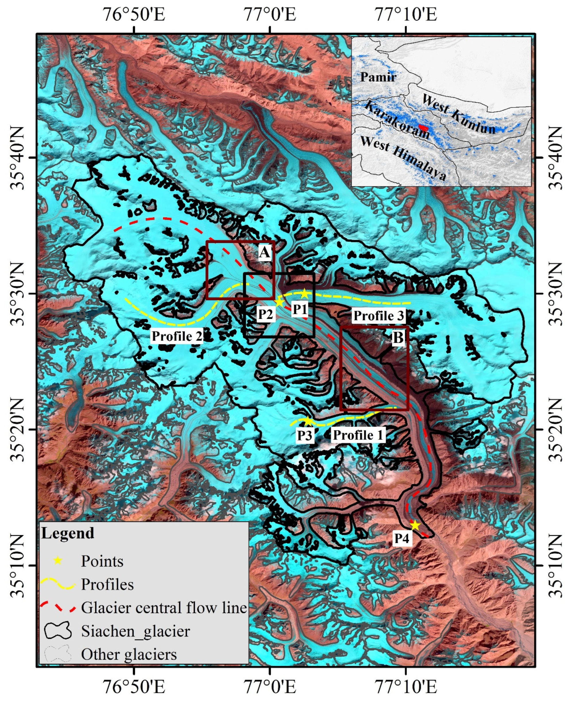
2. Study Region
3. Materials
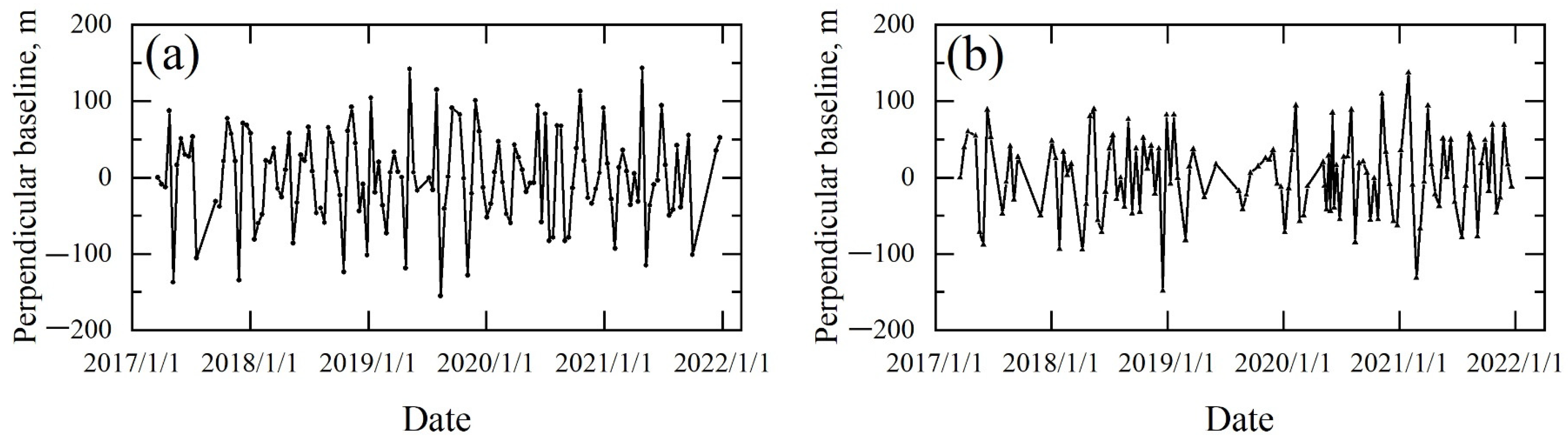
3.1. Sentinel-1 Data
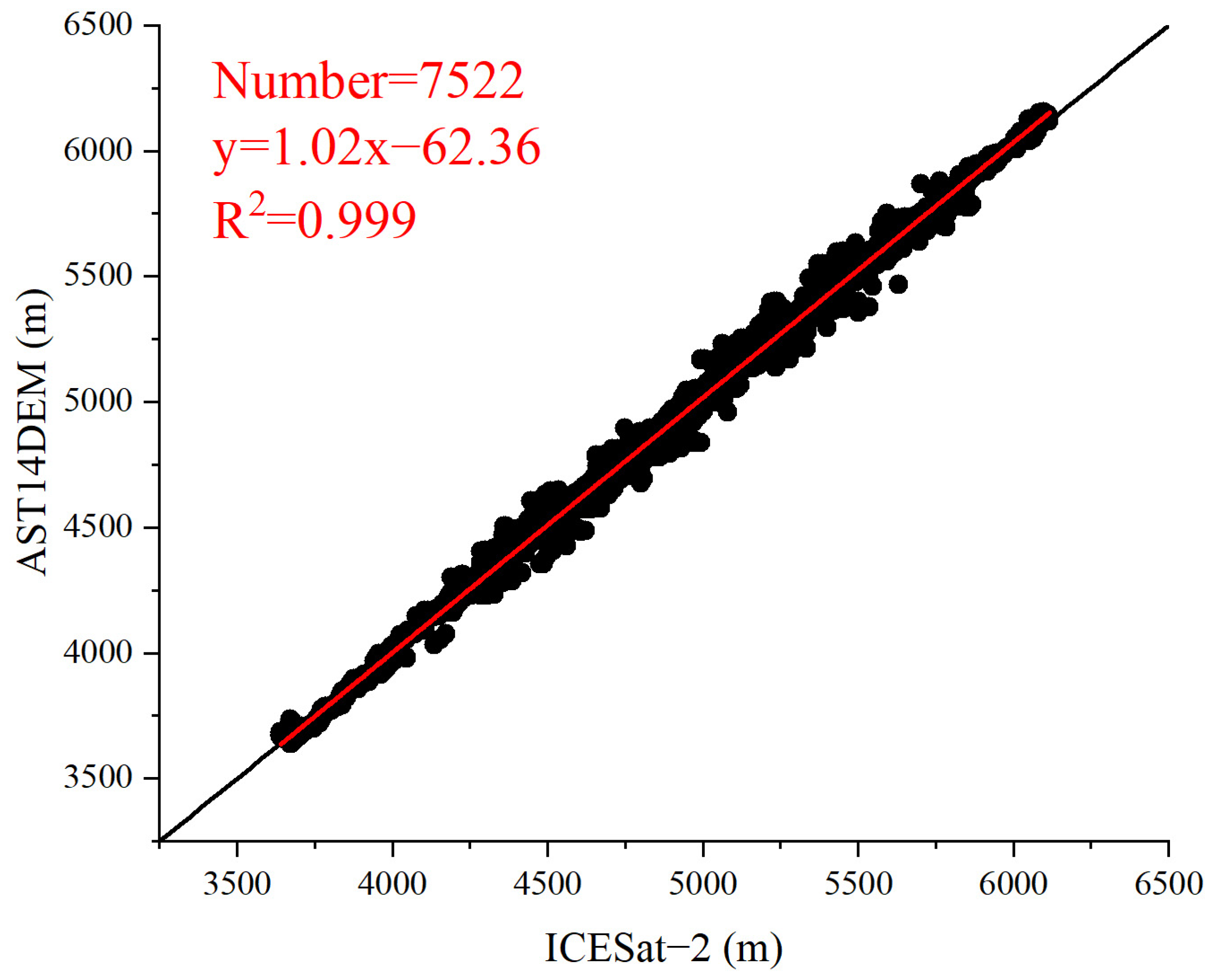
3.2. Digital Elevation Model
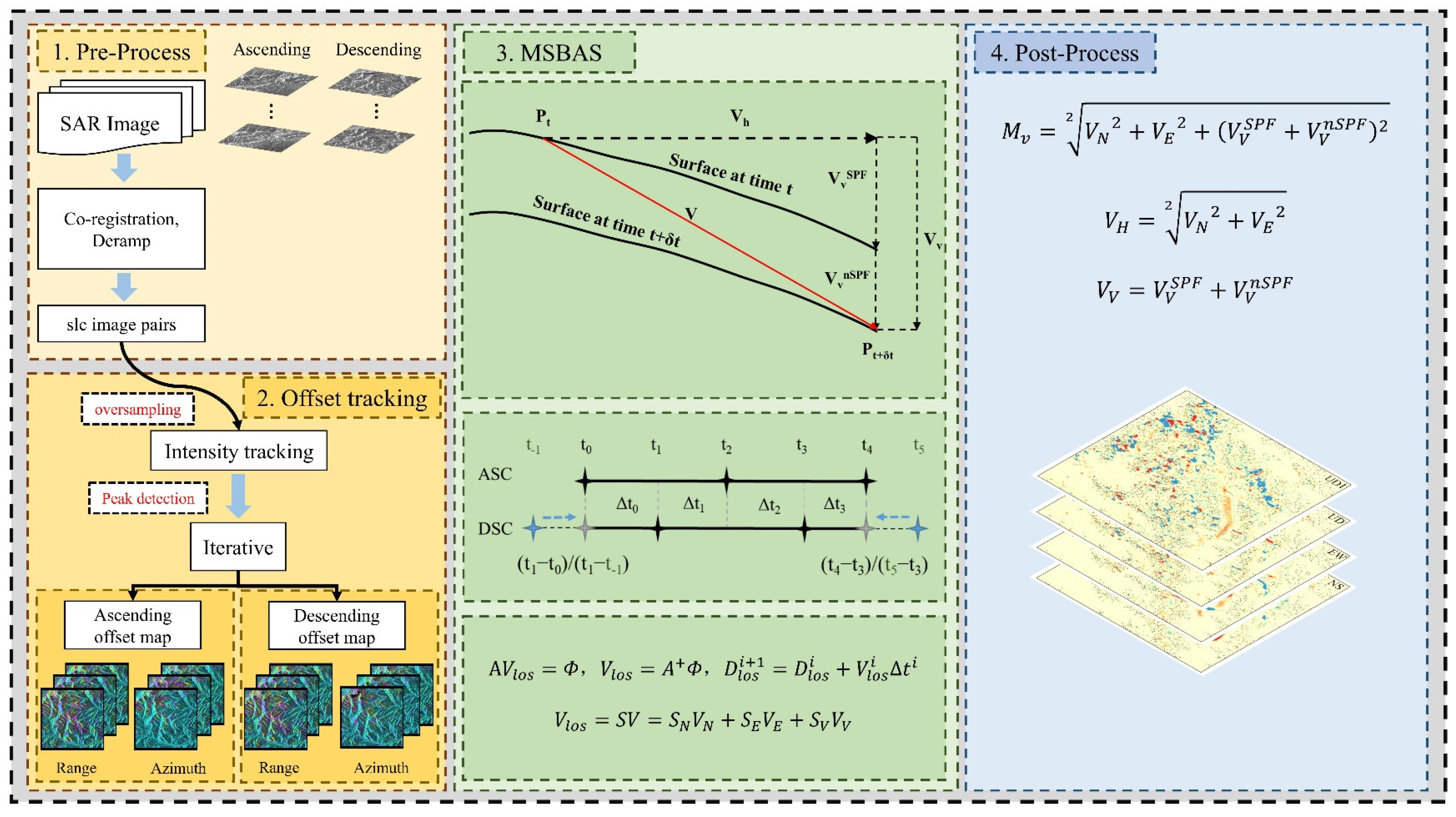
4. Methodology
4.1. Glacier Outlines Delineation
4.2. Glacier Velocity Retrieval
4.2.1. Offset Tracking
4.2.2. Multidimensional Small Baselines Subset (MSBAS)
4.3. Estimation of Glacier Mass Balance
4.4. Accuracy Assessment
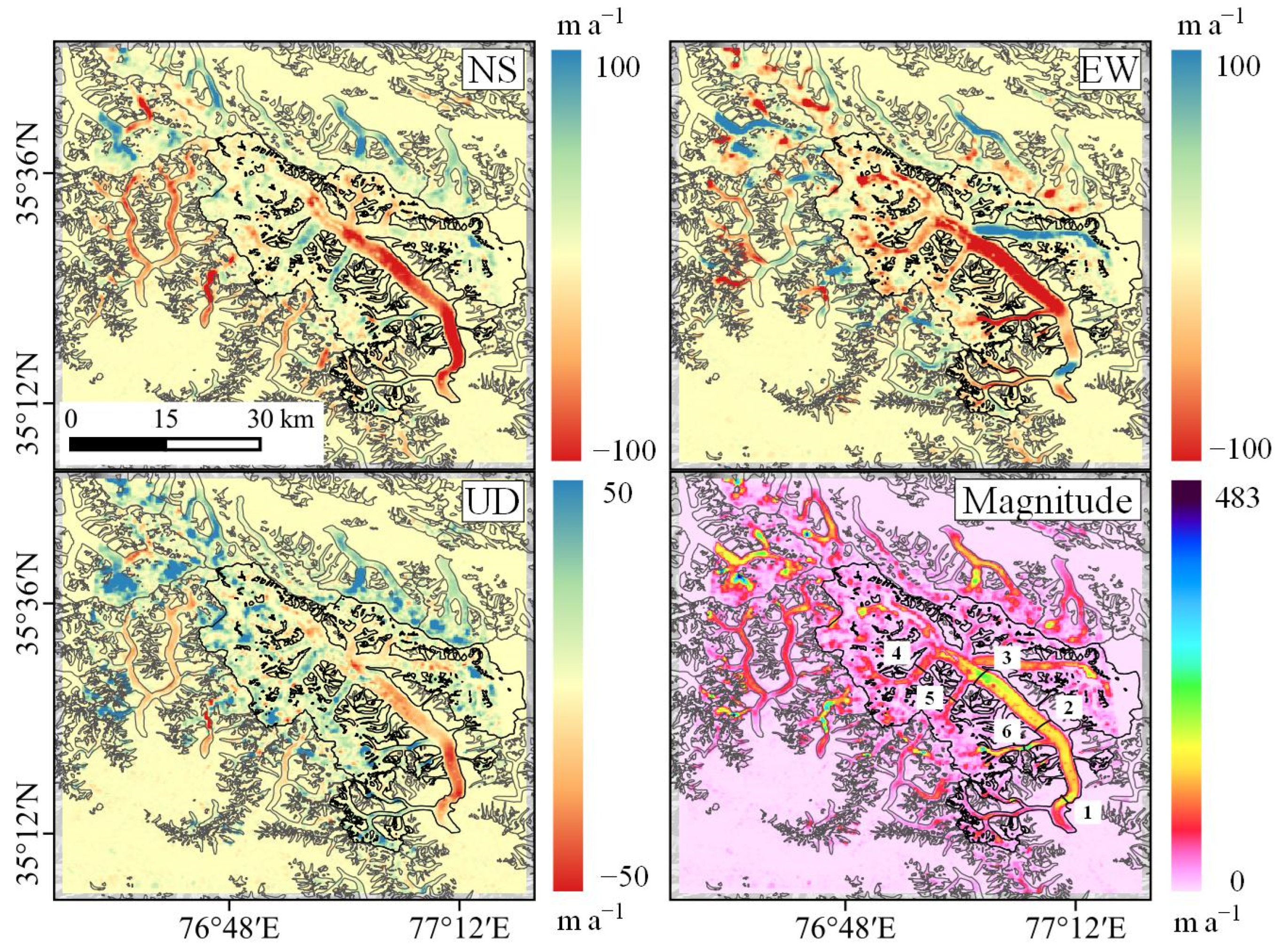
4.4.1. Accuracy Assessment of the Flow Velocity Components
4.4.2. Accuracy Assessment of the Magnitude of Linear Flow Velocity and Surface Elevation Change
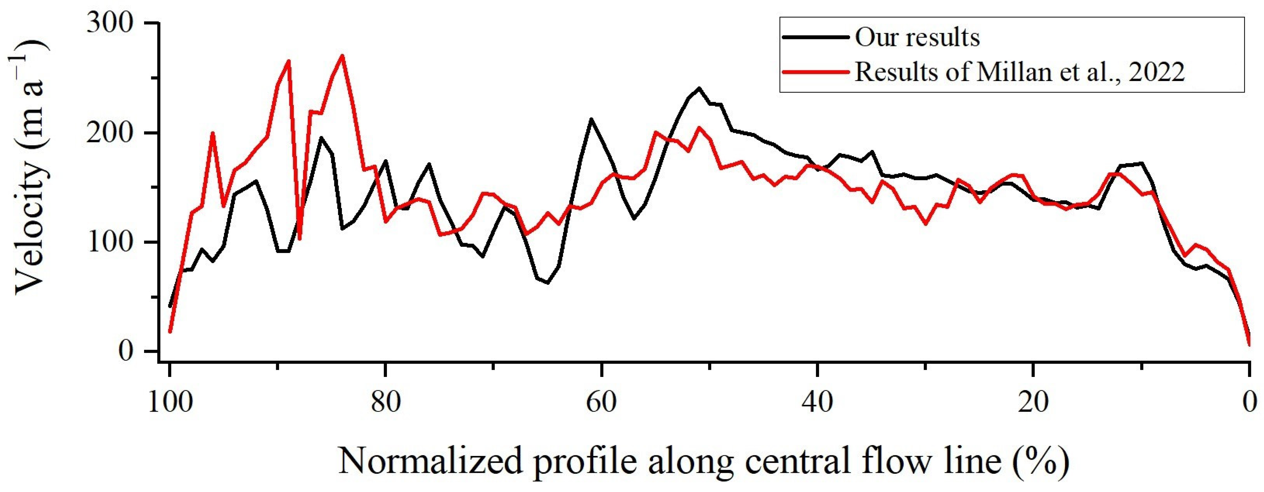
5. Results and Discussion
6. Conclusions
Author Contributions
Funding
Data Availability Statement
Acknowledgments
Conflicts of Interest
References
- Vaughan, D.G.; Comiso, J.; Allison, I.; Carrasco, J.; Kaser, G.; Kwok, R.; Holland, D. Observations: Cryosphere. In Climate Change 2013: The Physical Science Basis. Contribution of Working Group I to the Fifth Assessment Report of the Intergovernmental Panel on Climate Change; Stocker, T.F., Qin, D., Plattner, G.K., Tignor, M., Allen, S.K., Boschung, J., Nauels, A., Eds.; Cambridge University Press: Cambridge, UK; New York, NY, USA, 2013. [Google Scholar]
- Jiang, Z.; Liu, S.; Peters, J.; Lin, J.; Long, S.; Han, Y.; Wang, X. Analyzing Yengisogat Glacier Surface Velocities with ALOS PALSAR Data Feature Tracking, Karakoram, China. Environ. Earth Sci. 2012, 67, 1033–1043. [Google Scholar] [CrossRef]
- Bhattacharya, A.; Bolch, T.; Mukherjee, K.; King, O.; Menounos, B.; Kapitsa, V.; Neckel, N.; Yang, W.; Yao, T. High Mountain Asian Glacier Response to Climate Revealed by Multi-Temporal Satellite Observations since the 1960s. Nat. Commun. 2021, 12, 4133. [Google Scholar] [CrossRef] [PubMed]
- Immerzeel, W.W.; Pellicciotti, F.; Bierkens, M.F.P. Rising River Flows throughout the Twenty-First Century in Two Himalayan Glacierized Watersheds. Nat. Geosci. 2013, 6, 742–745. [Google Scholar] [CrossRef]
- Brun, F.; Berthier, E.; Wagnon, P.; Kääb, A.; Treichler, D. A Spatially Resolved Estimate of High Mountain Asia Glacier Mass Balances from 2000 to 2016. Nat. Geosci. 2017, 10, 668–673. [Google Scholar] [CrossRef] [PubMed]
- Dehecq, A.; Gourmelen, N.; Gardner, A.S.; Brun, F.; Goldberg, D.; Nienow, P.W.; Berthier, E.; Vincent, C.; Wagnon, P.; Trouvé, E. Twenty-First Century Glacier Slowdown Driven by Mass Loss in High Mountain Asia. Nat. Geosci. 2019, 12, 22–27. [Google Scholar] [CrossRef]
- Goldstein, R.M.; Engelhardt, H.; Kamb, B.; Frolich, R.M. Satellite Radar Interferometry for Monitoring Ice Sheet Motion: Application to an Antarctic Ice Stream. Science 1993, 262, 1525–1530. [Google Scholar] [CrossRef]
- Joughin, I.R.; Kwok, R.; Fahnestock, M.A. Interferometric Estimation of Three-Dimensional Ice-Flow Using Ascending and Descending Passes. IEEE Trans. Geosci. Remote Sens. 1998, 36, 25–37. [Google Scholar] [CrossRef]
- Strozzi, T.; Luckman, A.; Murray, T.; Wegmuller, U.; Werner, C.L. Glacier Motion Estimation Using SAR Offset-Tracking Procedures. IEEE Trans. Geosci. Remote Sens. 2002, 40, 2384–2391. [Google Scholar] [CrossRef]
- Usman, M.; Furuya, M. Interannual Modulation of Seasonal Glacial Velocity Variations in the Eastern Karakoram Detected by ALOS-1/2 Data. J. Glaciol. 2018, 64, 465–476. [Google Scholar] [CrossRef]
- Guo, L.; Li, J.; Li, Z.; Wu, L.; Li, X.; Hu, J.; Li, H.; Li, H.; Miao, Z.; Li, Z. The Surge of the Hispar Glacier, Central Karakoram: SAR 3-D Flow Velocity Time Series and Thickness Changes. J. Geophys. Res. Solid Earth 2020, 125, e2019JB018945. [Google Scholar] [CrossRef]
- Guan, W.; Cao, B.; Pan, B.; Chen, R.; Shi, M.; Li, K.; Zhao, X.; Sun, X. Updated Surge-Type Glacier Inventory in the West Kunlun Mountains, Tibetan Plateau, and Implications for Glacier Change. J. Geophys. Res. Earth Surf. 2022, 127, e2021JF006369. [Google Scholar] [CrossRef]
- Wang, Q.; Fan, J.; Zhou, W.; Tong, L.; Guo, Z.; Liu, G.; Yuan, W.; Sousa, J.J.; Perski, Z. 3D Surface Velocity Retrieval of Mountain Glacier Using an Offset Tracking Technique Applied to Ascending and Descending SAR Constellation Data: A Case Study of the Yiga Glacier. Int. J. Digit. Earth 2019, 12, 614–624. [Google Scholar] [CrossRef]
- Horgan, H.J.; Anderson, B.; Alley, R.B.; Chamberlain, C.J.; Dykes, R.; Kehrl, L.M.; Townend, J. Glacier Velocity Variability Due to Rain-Induced Sliding and Cavity Formation. Earth Planet. Sci. Lett. 2015, 432, 273–282. [Google Scholar] [CrossRef]
- Fey, C.; Krainer, K. Analyses of UAV and GNSS Based Flow Velocity Variations of the Rock Glacier Lazaun (Ötztal Alps, South Tyrol, Italy). Geomorphology 2020, 365, 107261. [Google Scholar] [CrossRef]
- Bearzot, F.; Garzonio, R.; Di Mauro, B.; Colombo, R.; Cremonese, E.; Crosta, G.B.; Delaloye, R.; Hauck, C.; Morra Di Cella, U.; Pogliotti, P.; et al. Kinematics of an Alpine Rock Glacier from Multi-Temporal UAV Surveys and GNSS Data. Geomorphology 2022, 402, 108116. [Google Scholar] [CrossRef]
- Copland, L.; Pope, S.; Bishop, M.P.; Shroder, J.F.; Clendon, P.; Bush, A.; Kamp, U.; Seong, Y.B.; Owen, L.A. Glacier Velocities across the Central Karakoram. Ann. Glaciol. 2009, 50, 41–49. [Google Scholar] [CrossRef]
- Nobakht, M.; Motagh, M.; Wetzel, H.-U.; Roessner, S.; Kaufmann, H. The Inylchek Glacier in Kyrgyzstan, Central Asia: Insight on Surface Kinematics from Optical Remote Sensing Imagery. Remote Sens. 2014, 6, 841–856. [Google Scholar] [CrossRef]
- Kääb, A.; Strozzi, T.; Bolch, T.; Caduff, R.; Trefall, H.; Stoffel, M.; Kokarev, A. Inventory and Changes of Rock Glacier Creep Speeds in Ile Alatau and Kungöy Ala-Too, Northern Tien Shan, since the 1950s. Cryosphere 2021, 15, 927–949. [Google Scholar] [CrossRef]
- Immerzeel, W.W.; Kraaijenbrink, P.D.A.; Shea, J.M.; Shrestha, A.B.; Pellicciotti, F.; Bierkens, M.F.P.; de Jong, S.M. High-Resolution Monitoring of Himalayan Glacier Dynamics Using Unmanned Aerial Vehicles. Remote Sens. Environ. 2014, 150, 93–103. [Google Scholar] [CrossRef]
- Wang, P.; Li, H.; Li, Z.; Liu, Y.; Xu, C.; Mu, J.; Zhang, H. Seasonal Surface Change of Urumqi Glacier No. 1, Eastern Tien Shan, China, Revealed by Repeated High-Resolution UAV Photogrammetry. Remote Sens. 2021, 13, 3398. [Google Scholar] [CrossRef]
- Samsonov, S.; Tiampo, K.; Cassotto, R. SAR-Derived Flow Velocity and Its Link to Glacier Surface Elevation Change and Mass Balance. Remote Sens. Environ. 2021, 258, 112343. [Google Scholar] [CrossRef]
- Łukosz, M.A.; Hejmanowski, R.; Witkowski, W.T. Evaluation of ICEYE Microsatellites Sensor for Surface Motion Detection—Jakobshavn Glacier Case Study. Energies 2021, 14, 3424. [Google Scholar] [CrossRef]
- Michel, R.; Avouac, J.-P.; Taboury, J. Measuring Ground Displacements from SAR Amplitude Images: Application to the Landers Earthquake. Geophys. Res. Lett. 1999, 26, 875–878. [Google Scholar] [CrossRef]
- Leprince, S.; Barbot, S.; Ayoub, F.; Avouac, J.P. Automatic and Precise Orthorectification, Coregistration, and Subpixel Correlation of Satellite Images, Application to Ground Deformation Measurements. IEEE Trans. Geosci. Remote Sens. 2007, 45, 1529–1558. [Google Scholar] [CrossRef]
- Pattyn, F.; Derauw, D. Ice-Dynamic Conditions of Shirase Glacier, Antarctica, Inferred from ERS SAR Interferometry. J. Glaciol. 2002, 48, 559–565. [Google Scholar] [CrossRef]
- Pathier, E.; Fielding, E.J.; Wright, T.J.; Walker, R.; Parsons, B.E.; Hensley, S. Displacement Field and Slip Distribution of the 2005 Kashmir Earthquake from SAR Imagery. Geophys. Res. Lett. 2006, 33. [Google Scholar] [CrossRef]
- Sansosti, E.; Berardino, P.; Bonano, M.; Calò, F.; Castaldo, R.; Casu, F.; Manunta, M.; Manzo, M.; Pepe, A.; Pepe, S.; et al. How Second Generation SAR Systems Are Impacting the Analysis of Ground Deformation. Int. J. Appl. Earth Obs. Geoinf. 2014, 28, 1–11. [Google Scholar] [CrossRef]
- Wegmüller, U.; Werner, C. Gamma SAR Processor and Interferometry Software. In Proceedings of the 3rd ERS Symposium, Florence, Italy, 17–21 March 1997. [Google Scholar]
- Pepe, A.; Solaro, G.; Calò, F.; Dema, C. A Minimum Acceleration Approach for the Retrieval of Multiplatform InSAR Deformation Time Series. IEEE J. Sel. Top. Appl. Earth Obs. Remote Sens. 2016, 9, 3883–3898. [Google Scholar] [CrossRef]
- Samsonov, S.; d’Oreye, N. Multidimensional Time-Series Analysis of Ground Deformation from Multiple InSAR Data Sets Applied to Virunga Volcanic Province. Geophys. J. Int. 2012, 191, 1095–1108. [Google Scholar] [CrossRef]
- Millan, R.; Mouginot, J.; Rabatel, A.; Morlighem, M. Ice Velocity and Thickness of the World’s Glaciers. Nat. Geosci. 2022, 15, 124–129. [Google Scholar] [CrossRef]
- Agarwal, V.; Bolch, T.; Syed, T.H.; Pieczonka, T.; Strozzi, T.; Nagaich, R. Area and Mass Changes of Siachen Glacier (East Karakoram). J. Glaciol. 2017, 63, 148–163. [Google Scholar] [CrossRef]
- Kumar, A.; Negi, H.S.; Kumar, K. Long-Term Mass Balance Modelling (1986–2018) and Climate Sensitivity of Siachen Glacier, East Karakoram. Environ. Monit. Assess. 2020, 192, 368. [Google Scholar] [CrossRef] [PubMed]
- Negi, H.S.; Kumar, A.; Kanda, N.; Thakur, N.K.; Singh, K.K. Status of Glaciers and Climate Change of East Karakoram in Early Twenty-First Century. Sci. Total Environ. 2021, 753, 141914. [Google Scholar] [CrossRef]
- Shean, D.E.; Alexandrov, O.; Moratto, Z.M.; Smith, B.E.; Joughin, I.R.; Porter, C.; Morin, P. An Automated, Open-Source Pipeline for Mass Production of Digital Elevation Models (DEMs) from Very-High-Resolution Commercial Stereo Satellite Imagery. ISPRS J. Photogramm. Remote Sens. 2016, 116, 101–117. [Google Scholar] [CrossRef]
- Paul, F.; Bolch, T.; Briggs, K.; Kääb, A.; McMillan, M.; McNabb, R.; Nagler, T.; Nuth, C.; Rastner, P.; Strozzi, T.; et al. Error Sources and Guidelines for Quality Assessment of Glacier Area, Elevation Change, and Velocity Products Derived from Satellite Data in the Glaciers_cci Project. Remote Sens. Environ. 2017, 203, 256–275. [Google Scholar] [CrossRef]
- Kääb, A.; Bolch, T.; Casey, K.; Heid, T.; Kargel, J.S.; Leonard, G.J.; Paul, F.; Raup, B.H. Glacier Mapping and Monitoring Using Multispectral Data. In Global Land Ice Measurements from Space; Kargel, J.S., Leonard, G.J., Bishop, M.P., Kääb, A., Raup, B.H., Eds.; Springer Praxis Books; Springer: Berlin/Heidelberg, Germany, 2014; pp. 75–112. ISBN 978-3-540-79818-7. [Google Scholar]
- Kaufmann, V.; Ladstaedter, R. Quantitative Analysis of Rock Glacier Creep by Means of Digital Photogrammetry Using Multi-Temporal Aerial Photographs: Two Case Studies in the Austrian Alps. In Proceedings of the 8th International Conference on Permafrost, Zürich, Switzerland, 21–25 July 2003. [Google Scholar]
- Scherler, D.; Leprince, S.; Strecker, M.R. Glacier-Surface Velocities in Alpine Terrain from Optical Satellite Imagery—Accuracy Improvement and Quality Assessment. Remote Sens. Environ. 2008, 112, 3806–3819. [Google Scholar] [CrossRef]
- Skvarca, P.; Kääb, A.; Haug, T. Monitoring Ice Shelf Velocities from Repeat MODIS and Landsat Data—A Method Study on the Larsen C Ice Shelf, Antarctic Peninsula, and 10 Other Ice Shelves around Antarctica. Cryosphere 2010, 4, 161–178. [Google Scholar] [CrossRef]
- Goldstein, R.M.; Zebker, H.A.; Werner, C.L. Satellite Radar Interferometry—Two-Dimensional Phase Unwrapping. Radio Sci. 1988, 23, 713–720. [Google Scholar] [CrossRef]
- Samsonov, S.V.; d’Oreye, N. Multidimensional Small Baseline Subset (MSBAS) for Two-Dimensional Deformation Analysis: Case Study Mexico City. Can. J. Remote Sens. 2017, 43, 318–329. [Google Scholar] [CrossRef]
- Kumar, V.; Venkataramana, G.; Høgda, K.A. Glacier Surface Velocity Estimation Using SAR Interferometry Technique Applying Ascending and Descending Passes in Himalayas. Int. J. Appl. Earth Obs. Geoinf. 2011, 13, 545–551. [Google Scholar] [CrossRef]
- Fialko, Y.; Simons, M.; Agnew, D. The Complete (3-D) Surface Displacement Field in the Epicentral Area of the 1999 MW7.1 Hector Mine Earthquake, California, from Space Geodetic Observations. Geophys. Res. Lett. 2001, 28, 3063–3066. [Google Scholar] [CrossRef]
- Samsonov, S. Topographic Correction for ALOS PALSAR Interferometry. IEEE Trans. Geosci. Remote Sens. 2010, 48, 3020–3027. [Google Scholar] [CrossRef]
- Reeh, N.; Madsen, S.N.; Mohr, J.J. Combining SAR Interferometry and the Equation of Continuity to Estimate the Three-Dimensional Glacier Surface-Velocity Vector. J. Glaciol. 1999, 45, 533–538. [Google Scholar] [CrossRef]
- Beedle, M.J.; Menounos, B.; Wheate, R. An Evaluation of Mass-Balance Methods Applied to Castle Creek Glacier, British Columbia, Canada. J. Glaciol. 2014, 60, 262–276. [Google Scholar] [CrossRef]
- Hansen, P.C.; O’Leary, D.P. The Use of the L-Curve in the Regularization of Discrete Ill-Posed Problems. SIAM J. Sci. Comput. 1993, 14, 1487–1503. [Google Scholar] [CrossRef]
- Zemp, M.; Huss, M.; Thibert, E.; Eckert, N.; McNabb, R.; Huber, J.; Barandun, M.; Machguth, H.; Nussbaumer, S.U.; Gärtner-Roer, I.; et al. Global Glacier Mass Changes and Their Contributions to Sea-Level Rise from 1961 to 2016. Nature 2019, 568, 382–386. [Google Scholar] [CrossRef]
- Huss, M. Density Assumptions for Converting Geodetic Glacier Volume Change to Mass Change. Cryosphere 2013, 7, 877–887. [Google Scholar] [CrossRef]
- Nuth, C.; Kääb, A. Co-Registration and Bias Corrections of Satellite Elevation Data Sets for Quantifying Glacier Thickness Change. Cryosphere 2011, 5, 271–290. [Google Scholar] [CrossRef]
- Gudmundsson, G.H.; Bauder, A. Towards an Indirect Determination of the Mass-Balance Distribution of Glaciers Using the Kinematic Boundary Condition. Geogr. Ann. Ser. A Phys. Geogr. 1999, 81, 575–583. [Google Scholar] [CrossRef]
- Millan, R.; Mouginot, J.; Rabatel, A.; Jeong, S.; Cusicanqui, D.; Derkacheva, A.; Chekki, M. Mapping Surface Flow Velocity of Glaciers at Regional Scale Using a Multiple Sensors Approach. Remote Sens. 2019, 11, 2498. [Google Scholar] [CrossRef]
- Cogley, J.G.; Arendt, A.A.; Bauder, A.; Braithwaite, R.J.; Hock, R.; Jansson, P.; Kaser, G.; Moller, M.; Nicholson, L.; Rasmussen, L.A.; et al. Glossary of Glacier Mass Balance and Related Terms; UNESCO/IHP: Paris, France, 2010. [Google Scholar]


| Track and Period | θ° | φ° | Image Pairs | |
|---|---|---|---|---|
| Ascending | 20170320~20211224 | 34 | 193 | 66 |
| Descending | 20170321~20211219 | 44 | 347 | 60 |
| Normalized Central Flow Line (%) | Correlation Coefficient * |
|---|---|
| 100 | 0.52 |
| 80 | 0.81 |
| 60 | 0.88 |
| 40 | 0.91 |
| 20 | 0.97 |
Disclaimer/Publisher’s Note: The statements, opinions and data contained in all publications are solely those of the individual author(s) and contributor(s) and not of MDPI and/or the editor(s). MDPI and/or the editor(s) disclaim responsibility for any injury to people or property resulting from any ideas, methods, instructions or products referred to in the content. |
© 2023 by the authors. Licensee MDPI, Basel, Switzerland. This article is an open access article distributed under the terms and conditions of the Creative Commons Attribution (CC BY) license (https://creativecommons.org/licenses/by/4.0/).
Share and Cite
Liang, Q.; Wang, N. Mountain Glacier Flow Velocity Retrieval from Ascending and Descending Sentinel-1 Data Using the Offset Tracking and MSBAS Technique: A Case Study of the Siachen Glacier in Karakoram from 2017 to 2021. Remote Sens. 2023, 15, 2594. https://doi.org/10.3390/rs15102594
Liang Q, Wang N. Mountain Glacier Flow Velocity Retrieval from Ascending and Descending Sentinel-1 Data Using the Offset Tracking and MSBAS Technique: A Case Study of the Siachen Glacier in Karakoram from 2017 to 2021. Remote Sensing. 2023; 15(10):2594. https://doi.org/10.3390/rs15102594
Chicago/Turabian StyleLiang, Qian, and Ninglian Wang. 2023. "Mountain Glacier Flow Velocity Retrieval from Ascending and Descending Sentinel-1 Data Using the Offset Tracking and MSBAS Technique: A Case Study of the Siachen Glacier in Karakoram from 2017 to 2021" Remote Sensing 15, no. 10: 2594. https://doi.org/10.3390/rs15102594