The Estimation of Maize Grain Protein Content and Yield by Assimilating LAI and LNA, Retrieved from Canopy Remote Sensing Data, into the DSSAT Model

Abstract

The assimilation of remote sensing data into mechanistic models of crop growth has become an available method for estimating yield. The objective of this study was to explore an effective assimilation approach for estimating maize grain protein content and yield using a canopy remote sensing data and crop growth model. Based on two years of field experiment data, the remote sensing inversion model using assimilation intermediate variables, namely leaf area index (LAI) and leaf nitrogen accumulation (LNA), was constructed with an R² greater than 0.80 and a low root-mean-square error (RMSE). The different data assimilation approaches showed that when the LAI and LNA variables were used together in the assimilation process (V_LAI+LNA), better accuracy was achieved for LNA estimations than the assimilation process using single variables of LAI or LNA (V_LAI or V_LNA). Similar differences in estimation accuracy were found in the maize yield and grain protein content (GPC) simulations. When the LAI and LNA were both intermediate variables in the assimilation process, the estimation accuracy of the yield and GPC were better than that of the assimilation process with only one variable. In summary, these results indicate that two physiological and biochemical parameters of maize retrieved from hyperspectral data can be combined with the crop growth model through the assimilation method, which provides a feasible method for improving the estimation accuracy of maize LAI, LNA, GPC and yield.

1. Introduction

Maize is one of the major food crops around world, providing energy for humans and animals, as well as being an important industrial raw material [1]. The accurate and timely assessment of real-time information on maize growth, yield and grain quality before harvest is critical for managing supply chains, food security, industrial development and farmers’ incomes [2,3,4,5]. Therefore, it is urgent to develop advanced prediction methods for maize growth, yield and grain quality. Remote sensing has been widely used in large-area crop yield estimation due to its advantages of non-contact data acquisition [6,7,8]. The use of assimilation methods to combine crop growth models with remote sensing data has become one of the more commonly used methods for estimating regional crop yields [9].

Crop models use mathematical formulas to express the relationship between crop growth status and environmental factors (soil nutrients, water, temperature and field management, etc.) [4,10,11,12,13,14]. They simulate changes in growth parameters and yields of crops from sowing to harvesting. The results of the model simulation are influenced by the initial conditions as well as the genetic and cultivar parameters, water and soil characteristics, meteorological data and human factors, which can bias crop growth models when applied to estimating yield over a large area [15]. With the improvement of sensor technology, the spatial and temporal resolution of remote sensing images can obtain more accurate crop growth information [16,17,18,19], which provides useful information for calibrating the variable simulation in crop models. Researchers have demonstrated that the assimilation of remote sensing data into crop models can improve the accuracy of crop yield simulation [7,12,20,21,22,23].

The combination of remote sensing data and crop models has achieved excellent results in increasing crop yields in a variety of crops [12,13,14,23,24,25,26,27]. Maas verified the initialization and parameterization model, which can make the simulated crop growth variables and yields closer to the actual observed values [28,29]. The researchers combined varieties of crop growth model, e.g., SUCROS [30] the Rotask [31], the World Food Research crop model [32], and remote sensing data to optimize crop and soil parameters for accurate estimation of crop yield and other physiological and biochemical parameters. The leaf area index (LAI) extracted from remote sensing data was the most commonly used intermediate variable in past studies. Through the observation system simulation experiment, the assimilation potential of LAI into the WOFOST crop growth model [33] and the CERES-Wheat model [34] were also verified, and this method usually improved the simulation accuracy of the LAI and further achieved more accurate crop yield estimation results. In addition, this kind of process was used with different kinds of remote sensing data. Jiang et al. applied the four-dimensional variational algorithm to the assimilation process of HJ-1A/B satellite images and the Decision Support System for Agrotechnology Transfer (DSSAT) model, and successfully estimated wheat yield at the regional level [35]. Furthermore, Huang et al. assimilated a time series of a 30 m resolution leaf area index (LAI) with a Kalman filter algorithm into the WOFOST model using the EnKF strategy, which provides a reliable and promising method for improving regional estimates of winter wheat yield with combing different kinds of satellite images [36]. In previous studies, LAI was an assimilation variable frequently used to improve the estimation accuracy of LAI and crop yield, but the accuracy of other output parameter variables of the model was not considered [37,38].

Previous studies have found that the assimilation process using two state variables can improve the estimation accuracy of crop state variables and final crop yield. Thorp et al. combined the crop growth model with the radiation transport model by using plant nitrogen accumulation and LAI as state variables, and improved the accuracy in estimation of nitrogen content, LAI, biomass and yield [39]. By considering prior information about expected climatic conditions during the growing season, the yield prediction performance was significantly improved by using both soil moisture and LAI as state variables for assimilation [12]. Jin et al. obtained reliable estimation results of biomass yield by using hyperspectral-retrieved biomass and canopy cover variables as assimilated state variables in the AquaCrop crop growth model [4]. Li et al. also verified a similar conclusion that when the LAI and N content parameters were used as state variables, grain N content and yield could be improved simultaneously, compared with a single state variable assimilation [40].

A large number of studies have focused on the assimilation of remote sensing data and crop models, screening sensitive variables and combinations to improve the accuracy of crop yield estimation, but few studies have focused on crop quality based on bivariate data assimilation methods. Thus, the targets of this study were: (i) to determine the appropriate vegetation indices for predicting the maize LAI and leaf nitrogen accumulation (LNA); (ii) to explore and compare the accuracy differences between the LAI and LNA estimations obtained from the remote sensing data and from the assimilation process, which involved the use of either the single variable, LAI or LNA (V_LAI or V_LNA), or the double variable, LAI and LNA (V_LAI+LNA); and (iii) to evaluate the accuracy of the assimilation method with different variables for estimating maize grain protein content (GPC) and yield.

2. Materials and Methods

2.1. Study Site

The crop growth experiments were conducted during the 2019 and 2020 maize growing season at the agricultural experimental base of Jilin University (43°56′41″N, 125°14′19″E), Changchun, China. Changchun belongs to the temperate continental semi-humid monsoon climate, with four distinct seasons. Warm and rainy summers are suitable for corn growth; winters are long and cold, and corn ripens once a year. Specific climate information can be obtained from similar previous studies [5].

2.2. Experimental Section

The spring maize planting management information, including the cultivars used, planting date and fertilizer levels, are presented in

Table 1. Spring maize cultivars and planting management information during 2019 and 2020.

Spring Maize Cultivars	Planting Date	Nitrogen Level (kg/ha)	Phosphorus Level (kg/ha)	Potassic Level (kg/ha)	Plant Densities (Plants/ha)
XianYu335	29 May 2019	0, 110, 220, 330, 440	100	100	potted test
XianYu335	29 May 2019	220	0, 50, 100, 150, 200	100	potted test
XianYu335	29 May 2019	220	100	0, 50, 100, 150, 200	potted test
Meilian158	8 May 2020	0, 110, 220, 330	100	100	62,500
Meilian158	8 May 2020	220	0, 50, 100, 150	100	62,500
Meilian158	8 May 2020	220	100	0, 50, 100, 150	62,500

. Five nitrogen levels, five phosphorus levels and five potassic levels were employed in both 2019 and 2020. The nitrogen fertilizer was urea (N, kg/ha), the phosphorus fertilizer was calcium superphosphate (P₂O₅, kg/ha) and the potassic fertilizer was potassium sulfate (K₂O, kg/ha). In order to obtain different LAI and LNA levels, the experiment in 2019 was a randomized complete block design with 30 replications of each treatment and the experiment in 2020 was a randomized complete block design with two replications. Pest and weed management were conducted according to the local practical standards for maize.

2.3. Field Data Acquisition

2.3.1. Canopy Hyperspectral Reflectance Data

Maize canopy hyperspectral reflectance data were observed at different growth periods of the maize. The data collection dates for 2019 were 19 July, 19 August, 28 August, 4 September, 12 September and 31 September, and the data collection dates for 2020 were 28 June, 9 July, 25 July, 7 August, 22 August and 27 September. Each treatment was observed twice in the same period. The hyperspectral reflectance was measured at a height of 1.0 m above the canopy with a nadir orientation under clear sky conditions at 10:00–14:00 local time using an ASD FieldSpec Pro (Analytical Spectral Devices, Boulder, CO, USA). This instrument detects electromagnetic radiation in the wavelength range of 350–2500 nm; a sampling interval of 1.4 nm between 350 and 1000 nm and 2 nm between 1000 and 2500 nm; and a spectral resolution of 3 nm (350–1000 nm), 8.5 nm 1000–1900 nm) and 6.5 nm (1900–2500 nm). The reflectance spectra for each canopy were calculated from the plant canopy radiance values divided by the white Spectralon panel radiance value. The ASD was configured to average 10 consecutively acquired spectra for each record. Three repeated measurements of the canopy spectral reflectance were performed for each experimental plot, and the average value of 30 records was calculated to represent the canopy reflectance of each plot in order to reduce the possible influence of the changing microclimate and soil conditions in the field.

2.3.2. Plant Measurements

The hyperspectral reflectance of the maize and the leaf area were recorded simultaneously. Leaf length (L) and leaf width (W) from every reflectance-measured plant were assessed using a ruler [41]. The total leaf area for the maize leaves was calculated as follows:

$$LAI=0.759{\sum }_{i=1}^m{L}_i\times W_i$$

(1)

where m is the total number of maize leaves in a certain ground area and i is a single maize leaf. The LAI was obtained by the ratio of total leaf area to per unit ground area.

Furthermore, the plant leaf corresponding to the spectral sampling position was collected and dried for calculating leaf dry weight (LDW) for per unit ground area. Leaf nitrogen content was determined via a micro-Keldjahl analysis. The LNA was expressed as:

$$LNA=LNC\times LDW$$

(2)

The grain yield was measured at the maturity of maize. Five 1 m² replicate plots were obtained from each plot, and five plants were sampled from each 1 m² plot to collect maize kernels. The collected grain was dried and weighed (±0.01 g) and uniformly converted into a weight with 14% moisture (kg/ha). The grain protein content (GPC, %) was obtained by multiplying the grain nitrogen content by 6.5 [42]. Overall, 30 and 24 samples were collected in 2019 and 2020, respectively.

2.3.3. Fundamental Data

The fundamental data related to the crop growth model included meteorological data, soil information and field management records. We directly used the meteorological data recorded at the stations around the study site. The data were retrieved from the National Information Center of the China Meteorological Administration (http://data.cma.cn/, accessed on 1 March 2021) and included the daily minimal temperature, maximal temperature, hours of sunshine and rainfall. The solar radiation was calculated from the hours of sunshine with the Angstrom formula.

The soil measurements were: soil texture, permanent wilting point, field capacity, volumetric water content at saturation, soil organic carbon, inorganic N, pH and bulk density [40]. Information on the crop management including sowing, irrigation and fertilizer application was also recorded.

2.3.4. LAI and LNA Estimation with Canopy Hyperspectral Data

Overall, 15 relevant hyperspectral vegetation indices from previous studies were selected to construct the LAI and LNA estimation models for the whole growth stage of maize in 2019 and 2020.

Table 2. Indices calculated for the LAI and LNA.

Vegetation Index	Name	Formula	Reference
REPvalue	REPvalue	dRREP/dλ	[43]
RVI	Ratio Vegetation Index	$R_{800}/R_{670}$	[44]
MSR	Modified Simple Ratio index	$(R_{800}/R_{670}-1)/\sqrt{(R_{800}/R_{670}+1)}$	[45]
WDRVI	Wide Dynamic Range Vegetation Index	$(0.1R_{890}-R_{670})/(0.1R_{890}+R_{670})$	[46]
NDCI	Normalized difference chlorophyll index	$\left(R_{708}-R_{665}\right)/\left(R_{708}+R_{665}\right)$	[47]
SIPI	Structure insensitive pigment index	$\left(R_{800}-R_{445}\right)/\left(R_{800}-R_{680}\right)$	[48]
PSDNa	Pigment-specific normalized difference-a	$\left(R_{800}-R_{680}\right)/\left(R_{800}+R_{680}\right)$	[49]
PSDNb	Pigment-specific normalized difference-b	$\left(R_{800}-R_{635}\right)/\left(R_{800}+R_{635}\right)$	[49]
PSDNc	Pigment-specific normalized difference-c	$\left(R_{800}-R_{470}\right)/\left(R_{800}+R_{470}\right)$	[49]
NDII	Normalized difference infrared index	$\left(R_{850}-R_{1650}\right)/\left(R_{850}+R_{1650}\right)$	[50]
NDMI	Normalized difference matter index	$\left(R_{1649}-R_{1722}\right)/\left(R_{1649}+R_{1722}\right)$	[51]
mSR705	Modified simple ratio 705	$\left(R_{750}-R_{445}\right)/\left(R_{705}-R_{445}\right)$	[52]
mND705	Modified normalized difference 705	$\left(R_{750}-R_{705}\right)/\left(R_{750}+2R_{445}\right)$	[53]
OSAVI	Optimized soil-adjusted vegetation index	$1.16\times \left(R_{800}-R_{670}\right)/\left(R_{800}+R_{670}+0.16\right)$	[54]
NDVI	Normalized difference vegetation index	$\left(R_{890}-R_{670}\right)/\left(R_{890}+R_{670}\right)$	[55]

Note: R represents the reflectance value for the specified band; dR_REP/dλ represents the first derivative of the red-edged band.

describes the information of indices details. In 2019, 144 samples were collected, and in 2020, 168 samples were collected. The linear or nonlinear relationships between the vegetation index and the LAI or LNA were established. We used randperm function of MATLAB to randomly extract 50% samples from the 2019 and 2020 data as calibration data sets (n = 156) and the rest were labeled as validation data sets (n = 156). The calibration data sets were used to analyze the relationships between the LAI, LNA, and each of the vegetation indices, and the validation data sets were used to evaluate the estimation accuracy of the calibration models.

2.4. Description of the DSSAT CERES-Maize Model

The DSSAT model (https://dssat.net/, accessed on 31 May 2018) has been in use for 40 years, and is used globally to solve complex crop-relevant scientific problems, such as global climate change, water and nutrient cycling and risk assessment for crop production [56]. The contained Cropping System Model integrates the genetic conditions, environmental conditions and management conditions to simulate the daily variation of a crop’s physiological and biochemical parameters such as the LAI, accumulated biomass, grain nitrogen content and yield [56,57].

In the DSSAT-CERES model, there are nine different stages according to the growth characteristics of spring maize [58,59]. The growth and senescence of leaf area were simulated per plant as single units. The growth of leaf area is determined by the growing degree days of each stage. The biomass accumulation was calculated by the leaf area, solar radiation and extinction coefficient. The biomass is distributed proportionally to different plant organs at different growth stages. The crop nitrogen requirement was affected by the biomass and critical nitrogen concentration. The process of plant nitrogen accumulation was simulated according to the crop’s nitrogen demand and potential soil nitrogen supply. The uptake of available soil nitrogen depends on soil moisture and soil nitrogen concentrations. The nitrogen content of maize grains is mainly determined by the accumulation of nitrogen and the proportion of dry matter in the grain filling stage. The grain dry matter is produced and migrated by photosynthesis in each stage, and the nitrogen comes mainly from direct root absorption at the grain filling stage and the re-transport of the stored nitrogen uptake. These two variables are constrained by maize variety, soil moisture and meteorological conditions.

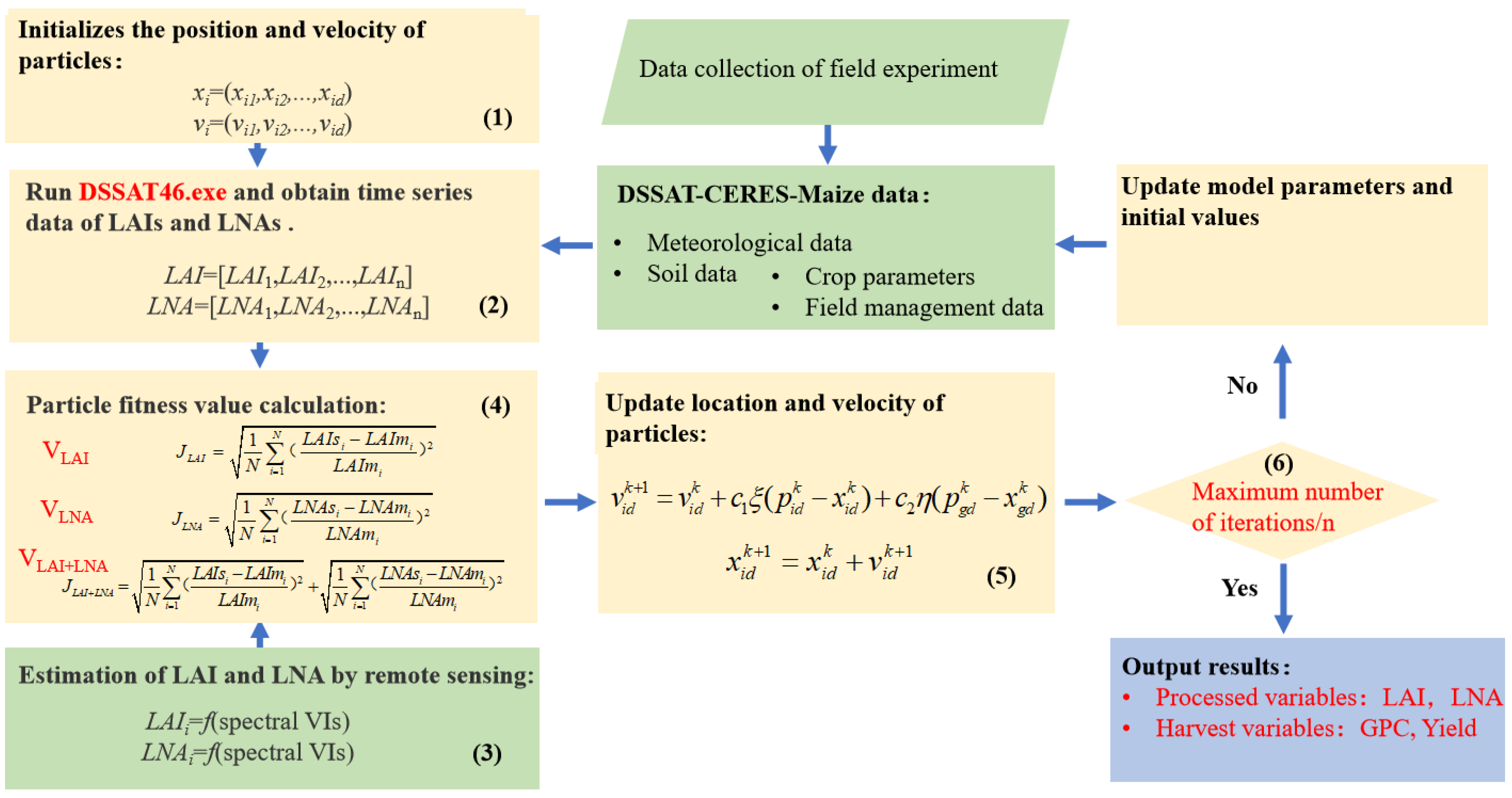
2.5. The Data Assimilation Method

Particle swarm optimization (PSO) is an evolutionary computation technique proposed by Eberhart and Kennedy based on bird-feeding studies [60]. It is based on a group cooperative stochastic search algorithm, which has the advantages of rapid convergence and high accuracy, and is often used in crop model optimization. PSO starts from a random solution and follows the current search to find the optimal value and the iteration to find the global optimal.

PSO takes a kind of massless particle (the number of study settings is 25) as an object, and endows the particle with two attributes—speed and position. Subsequently, it presents the speed and direction of movement, and each particle has a fitness value determined by the objective function to determine its own best position (P_obest), which can be seen as the particle’s own flight experience. Additionally, the particle also knows the best position (P_best) of all particles found so far (P_best is the best value in P_obest), which can be called the particle companion experience. The particle combines its own and its peer’s experience to determine the next movement, until the global optimal solution is determined. Figure 1 depicts the workflow of assimilating the canopy hyperspectral remote sensing data into the DSSAT models to estimate the maize LAI, LNA, yield and GPC. In order to evaluate the effect of different process variables involved in the assimilation process, three assimilation strategies were adopted: (i) with the LAI as the only process variable (V_LAI), (ii) with the LNA as the only process variable (V_LNA), and (iii) with both the LAI and LNA as process variables (V_LAI+LNA). The specific assimilation strategies were as follows:

(1)

Assign the initial values to the position and velocity of the particle. The initial conditions sowing density (PPOP), the fertilization amount (FAMN) and the results of the parameter sensitivity analysis of the DSSAT-CERES-Maize model (

Table 3. Initial value and tuning range of model parameters to be optimized.

Parameters	Initial Value	Range
PPOP (population of plant/m2)	6.5	5.5–9.5
FAMN (kg/ha)	200	0–400
P1 (°C)	200.9	170–280
P2	0.75	0.5–0.9
P5 (°C)	850.1	600–1100
G2	850.2	400–1100
G3 (mg/d)	10.97	4–11.5
PHINT (°C)	44.58	30–90
GDDE (day)	6	4–9
DSGFT (°C)	110	85–225
RUE	4.92	2–5
KCAN	0.45	0.45–0.9
SALB	0.18	0.088–0.132
SLUI (mm)	6	3–12
SLDR	0.9	0.01–0.95
SLRO	66	61–94
SLNF	1	0.72–1.08
SLPF	0.96	0.72–1.08

) were used as parameters to be optimized;

(2)

Run the DSSAT executable using the Rstudio software and retrieve the Time series simulation values for the LAI and LNA;

(3)

Perform the remote sensing inversion of the LAI and LNA. The spectral parameter models of the LAI and LNA are constructed;

(4)

Construct the fitness function. The fitness function is established by the LAIs and LNAs simulated by the DSSAT model and the LAIm and LNAm retrieved by the vegetation index. This function is used to determine the optimal input parameters of the model. In the assimilation strategy with only one process variable (V_LAI or V_LNA), the cost function is constructed based on only one variable (LAI or LNA). In addition, the two variables are both considered for building the fitness function in the assimilation strategy, V_LAI+LNA;

(5)

At each iteration, the P_obest and P_best are updated by changing the speed and position of each particle. C₁ and C₂ are equal to 2, and ρ and η are set to a random number between 0 and 1 [61];

(6)

The iteration terminates or continues the loop. The position of each particle is updated, and if the number of iterations (100) is not reached, redo step (2). If the last iteration is reached, the maize LAI, LNA, yield and GPC results are output. Figure S1 showed the final distribution range of each optimization parameter.

3. Results

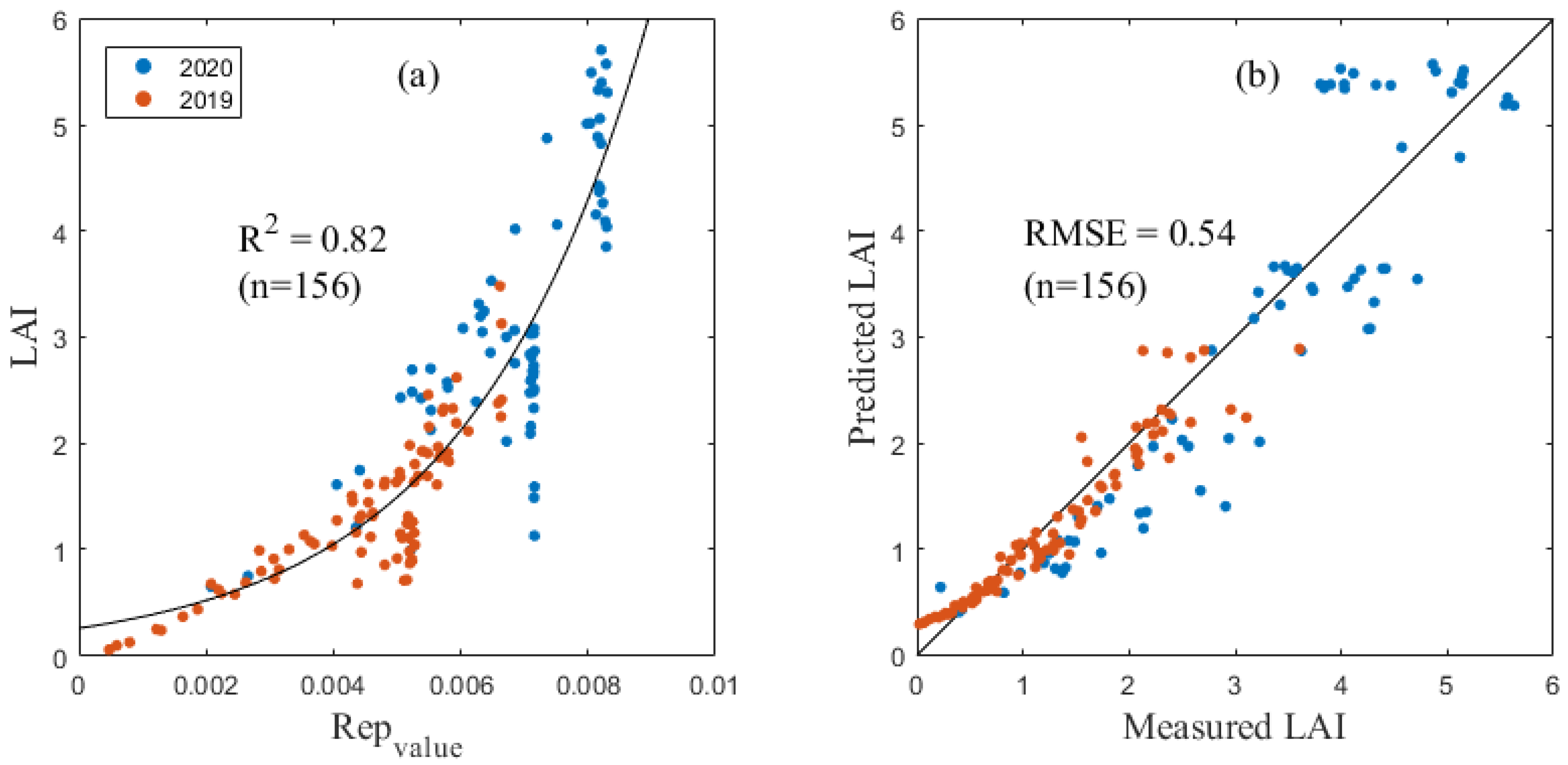
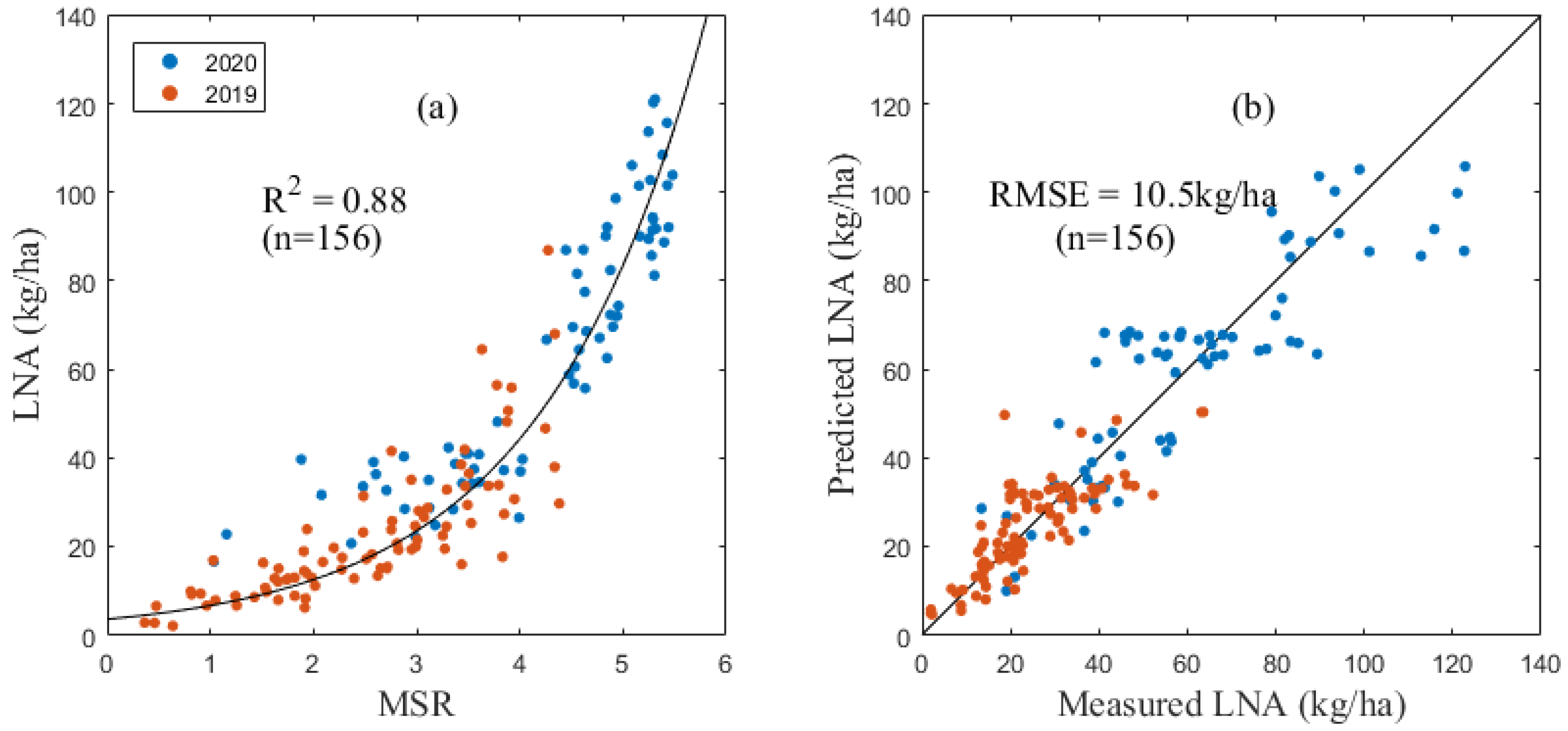
3.1. Estimating LAI and LNA Using Spectral Indices

The linear, exponential, logarithmic and power function models of each index and the respective target parameters were constructed, and the best estimation model was selected by the order of R² and the root-mean-square error (RMSE).

Table 4. The results of the spectral indices model for predicting the LAI.

Spectral Indices	LAI Model	R2	RMSE
REPvalue	y = 0.255e352.9x	0.82 **	0.54
NDII	y = 1.07e2.245x	0.80 **	0.59
NDCI	y = 75.96x + 9.12	0.79 **	0.63
OSAVI	y = 0.015e7.07x	0.77 **	0.76
NDMI	y = 0.1324e76.21x	0.72 **	0.81
MSR	y = 0.28e0.52x	0.72 **	0.81
SIPI	y = 10.99x + 13.91	0.71 **	0.8
WDRVI	y = 1.11e2.69x	0.70 **	0.82
RVI	y = 0.15x − 0.29	0.70 **	0.82

Note: x represents the value of spectral indices; y represents the value of the LAI (or LNA); ** represents p < 0.01.

and

Table 5. The results of the spectral indices model for predicting the LNA.

Spectral Indices	LNA Model	R2	RMSE (kg/ha)
MSR	y = 3.488e0.64x	0.85 **	10.71
OSAVI	y = 0.118e8.26x	0.83 **	11.01
WDRVI	y = 16.79e3.36x	0.82 **	11.25
PSDNc	y = 363.7x20.09	0.79 **	11.52
PSDNa	y = 228.7e13.47x	0.78 **	11.67
TVI	y = 2.86e0.144x	0.76 **	11.59
mSR705	y = 5.195x2.038	0.75 **	11.68
mND705	y = 330.4x4.575	0.74 **	11.83
PSDNb	y = 173.3x8.02	0.71 **	12.03

Note: x represents the value of spectral indices; y represents the value of the LAI (or LNA); ** represents p < 0.01.

introduce the optimal models for the prediction of the LAI and LNA.

The prediction model showed that the LAI or LNA was significantly correlated with the selected spectral index. Table 4 and Table 5, respectively, show correlation index models with R² values greater than 0.7 in the LAI and LNA estimation. Among them, the REP_value (Figure 2) and NDII had the best estimation effects on the maize LAI with an RMSE of 0.54 and 0.59, respectively.

There was also a good correlation between the LNA and various spectral indices. Among them, the MSR (Figure 3), OSAVI and WDRVI had the closest relationships with the LNA and were very sensitive to the change of the LNA value (R² equal 0.85, 0.83 and 0.82, respectively). The corresponding RMSE values of the model were 10.71 kg/ha, 11.01 kg/ha and 11.25 kg/ha, respectively. The MSR was selected to estimate the LNA of maize in this study.

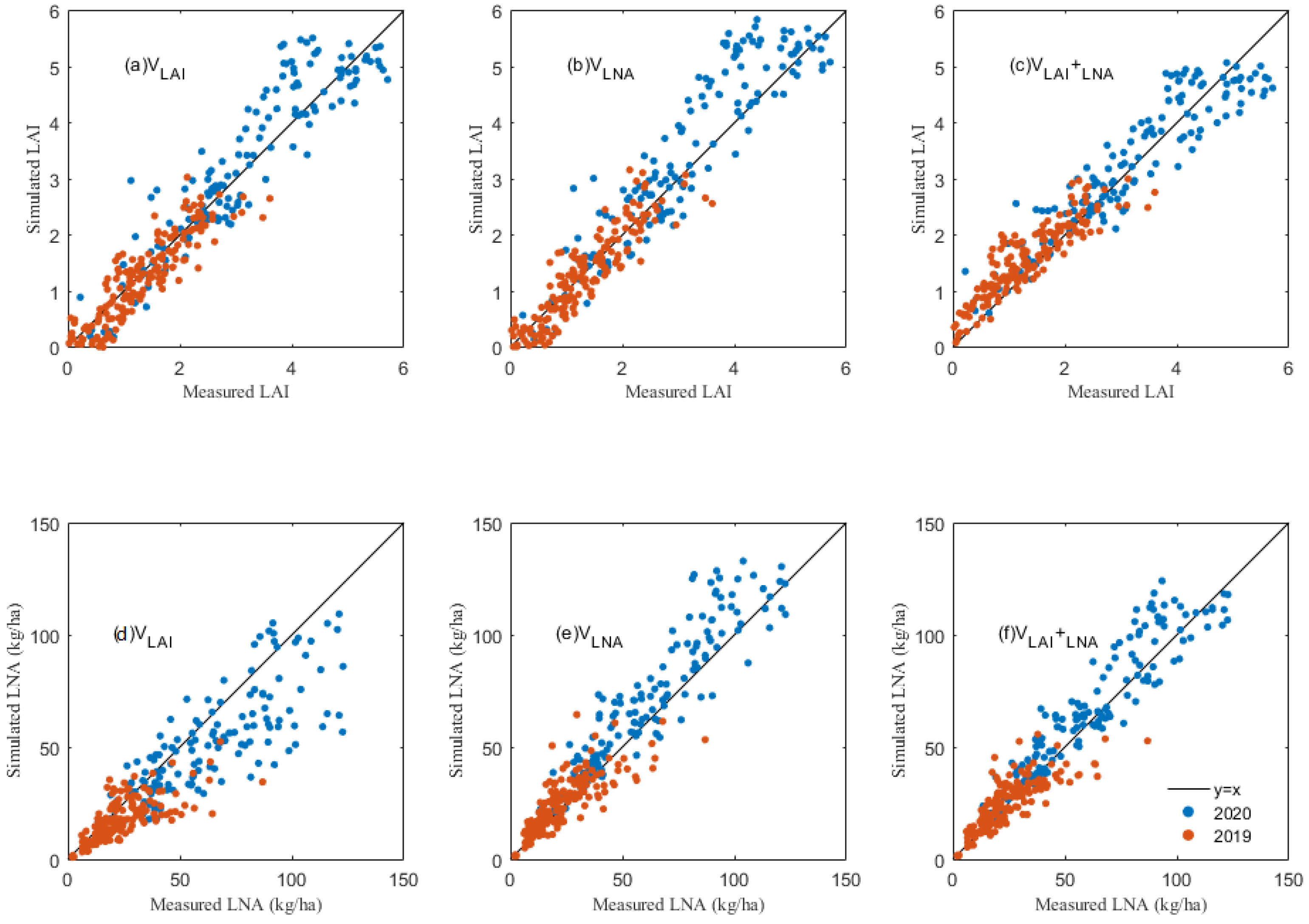
3.2. The LAI and LNA Simulation through Data Assimilating

The LAI and LNA values obtained from hyperspectral inversion were set as the intermediate variables in the assimilation process of the DSSAT model, and the PSO algorithm was used to optimize the model. The results showed that the LAI estimated by the data assimilation method was close to the actual measured value (Figure 4 and

Table 6. The relationships between the simulated and measured values of LAI.

	Year	n	R2	RMSE
VLAI	2020	144	0.811	0.582
	2019	168	0.761	0.363
VLNA	2020	144	0.738	0.685
	2019	168	0.787	0.343
VLAI+LNA	2020	144	0.853	0.513
	2019	168	0.699	0.408

). When the LAI was used as the only process variable (V_LAI), the simulated LAI after the model optimization was very consistent with the measured value (Figure 4a and Table 6), with R² values of 0.811 and 0.761 and RMSE values of 0.363 and 0.582, for 2019 and 2020, respectively. However, the estimated LAI obviously deviates from the measured LAI when the LNA was used as the only state variable (V_LNA) in 2020 (Figure 4b and Table 6), the R² values were 0.738 and 0.787 and the RMSE values were 0.343 and 0.685, in 2019 and 2020, respectively. When the LAI and LNA were combined as common intermediate variables, an excellent correlation between the estimated LAI and measured LAI was found in 2020 (Figure 4c), with R² and RMSE values of 0.853 and 0.531 (Table 6).

Additionally, the effects of the three assimilation methods (V_LAI, V_LNA and V_LAI+LNA) on the LNA simulation were compared. The LNA simulated by the V_LAI method had a poor correlation with the measured value (Figure 4d and

Table 7. The relationships between the simulated and measured values of LNA.

	Year	n	R2	RMSE (kg/ha)
VLAI	2020	144	0.455	20.442
	2019	168	0.343	11.482
VLNA	2020	144	0.720	14.646
	2019	168	0.615	8.787
VLAI+LNA	2020	144	0.824	11.618
	2019	168	0.661	8.253

), with R² values of 0.455 and 0.343 and RMSE values of 20.442 kg/ha and 11.482 kg/ha for 2020 and 2019, respectively. The simulated LNA in the V_LNA method had a better agreement with the measured value than the V_LAI (Figure 4e and Table 7), with R² values of 0.72 and 0.615 and RMSE values of 14.646 kg/ha and 8.787 kg/ha in 2020 and 2019, respectively. The best estimates of the LNA were found in the V_LAI+LNA approach, with R² values of 0.824 and 0.661 and RMSE values at 2.71 ton/ha and 2.81 ton/ha in 2019 and 2020, respectively (Figure 4f and Table 7).

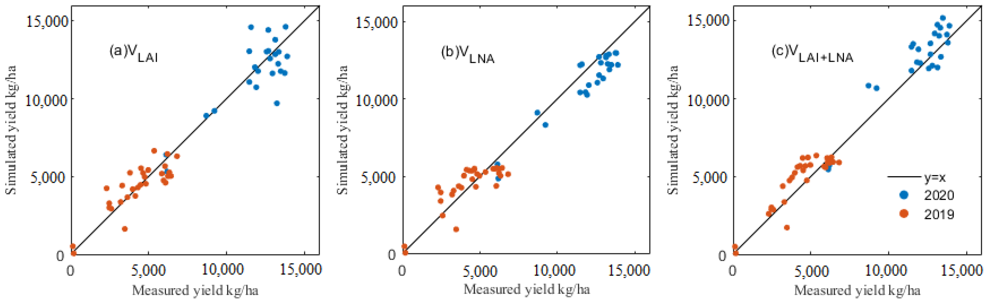
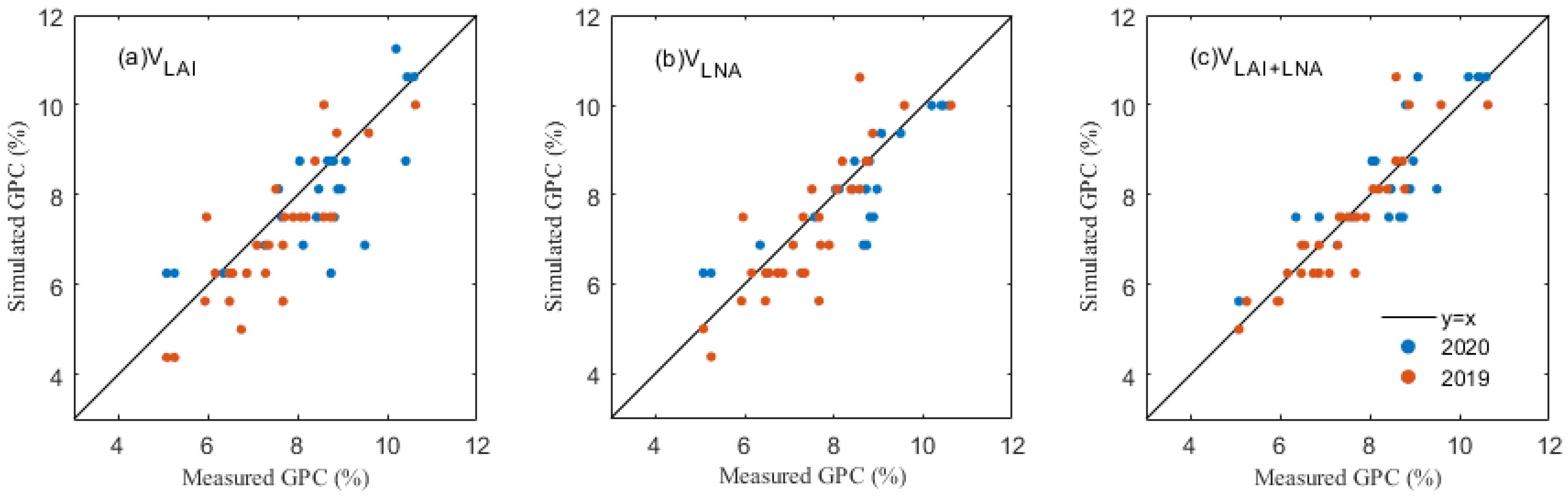
3.3. The Estimation of Yield and GPC

Based on the remote sensing data of each period of maize growth, the PSO algorithm was used to optimize the maize growth model (DSSAT-CERES-MAIZE), and thus, an effective simulation of the maize GPC and yield was obtained. Figure 5 and Figure 6 show the simulated and true values of the maize GPC and yield under various assimilation methods. The potting sand experiment in 2019 showed a relatively low yield. Field trials with fertile soils in 2020 harvested higher yields. In two years of experiments, the simulated results and ground-measured values of the maize GPC and yield data showed consistency under various assimilation methods. The results described that the V_LNA for 2020 (R², 0.754; RMSE, 1061.378 kg/ha) and the V_LAI for 2019 (R², 0.721; RMSE, 903.091 kg/ha) were better able to estimate maize yield than the V_LAI method for 2020 (R², 0.609; RMSE, 1339.339 kg/ha) and the V_LNA for 2019 (R², 0.674; RMSE, 976.681 kg/ha) (Figure 5,

Table 8. Simulation results of grain protein and yield under different assimilation processes.

			Yield		Protein Content
Methods	Year	n	R2	RMSE (kg/ha)	R2	RMSE (%)
VLAI	2020	24	0.609	1339.339	0.466	1.048
	2019	30	0.721	903.091	0.493	0.878
VLNA	2020	24	0.754	1061.378	0.665	0.830
	2019	30	0.674	976.681	0.577	0.802
VLAI+LNA	2020	24	0.726	1120.934	0.711	0.771
	2019	30	0.735	879.648	0.759	0.605

). V_LAI+LNA contributed the RMSE of 879.648 kg/ha for 2019 and 1120.934 kg/ha for 2020, with an R² of 0.735 for 2019 and 0.726 for 2020. By contrast, the data assimilation method using multiple state variables more accurately estimated maize yield than the single-state variable method.

In the simulation of maize grain protein content, the simulation results of the three assimilation methods were similar to the results of the yield simulation, and the simulated values were well correlated with the ground measurements (Figure 6, Table 8). A comparison of the assimilation methods involving the different state variables shows different assimilation strategies, and shows the accuracy of V_LAI for 2019 (R², 0.493 and RMSE, 0.878%) and 2020 (R², 0.466 and RMSE, 1.048%). The results of the bivariate assimilation strategy show that the simulated values obtained by the V_LAI+LNA method are similar to the measured values with 2019 (R², 0.759 and RMSE, 0.605%) and 2020 (R², 0.711 and RMSE, 0.771%), and significantly better than the simulated values obtained by univariate assimilation strategy. This further illustrates the simulated advantage of the LAI and LNA binding as an intermediate variable in the assimilation process for the maize GPC.

4. Discussion

The spectral indices, LAI and LNA, were measured during the 2019 and 2020 spring maize experiment. The selected spectral indices have their own characteristics to retrieve the LAI and LNA (Table 4 and Table 5). All the spectral indices were calculated with the characteristic bands of the canopy hyperspectral of the maize, which can represent the maize plants’ physiological structures and provide nutritional information about them. The regression between the Rep_value and the LAI (Figure 3) was more accurate than with the other indices. The Rep_value was sensitive to the change of chlorophyll content in the plants’ leaves. The chlorophyll content of the plants was closely related to the change in the LAI. The study tried to construct the regression relationship between the Rep_value and the LAI of the maize plants (R², RMSE = 0.82, 0.54). Meanwhile, the estimation accuracy of the LNA based on the MSR (R², RMSE = 0.85, 10.71 kg/ha) was better than the other indices. According to the construction formula of the MSR, the ratio between the reflectance of the near-infrared band and the red band can reduce the noise caused by the synchronous increase and decrease in reflectance of these two bands [61], and alleviate the influence of the saturation effect of the gradually increasing LAI on the cumulative amount of leaf nitrogen [45]. We compared the accuracy of the model with multiple data sets, and the prediction accuracy was similar. The model built using 50% sample data has the lowest accuracy, so we choose this proportion to complete the model description, so as to represent more situations (Tables S1 and S2).

Additionally, two years of experiments can show that the prediction results are applicable to different fertilizer rates and maize varieties. While the hyperspectral data of the maize in the experimental area were obtained, the LAI and LNA were collected accordingly. Previous studies have shown that by using satellite spectral response functions, the hyperspectral data can be calculated as satellite data vegetation indices for subsequent regional applications [62]. Therefore, future regional applications of this study also need to consider the influence of factors such as the atmospheric radiation transfer effects on the acquisition of satellite data. In this study, there were differences in the hyperspectral data of maize between the 2019 and 2020 experiments, which were not specifically introduced. The differences may be due to the influence of the soil type and maize planting density over the two-year experiment, which brings uncertainty to the generalization of the LAI and LNA estimation models. In future studies, we will further combine the different soil types and maize planting interval conditions to explore a better inversion method for the crop biochemical parameters.

The three methods used in this study to assimilate remote sensing data into the DSSAT model show that no matter whether the LAI and LNA appear as univariate or combined variables, the involved variables can be accurately estimated, which was also found in previous studies [4,30,40]. However, the simulation accuracy of the variable not involved in the assimilation process (LNA or LAI) is poor under the univariate assimilation methods (V_LAI or V_LNA) upon most occasions (Figure 4, Table 6 and Table 7). For example, the RMSE of the LNA in the V_LAI assimilation method were 20.442 kg/ha and 11.482 kg/ha in 2020 and 2019, much higher than that of the V_LNA (RMSE = 14.646 kg/ha and 8.787 kg/ha). Similarly, the error (RMSE = 0.685) between the simulated LAI values and the measured LAI values during the V_LNA assimilation was also greater than that of V_LAI (RMSE = 0.582) in 2020. Therefore, when only one intermediate variable is used for the DSSAT model optimization, the simulation accuracy of variable not involved in the assimilation is likely to decline. When the LAI and LNA take bivariate cooperation as the assimilation variable in the assimilation process of the DSSAT model, the simulation results of these two variables achieve quite a high accuracy, especially in 2020 (Figure 4, Table 6 and Table 7). In the process of V_LAI+LNA assimilation, the simulation accuracy of the LNA was surprisingly higher than the best effect of the V_LAI and V_LNA process variables’ simulation in both two years. The leaf area index is an important parameter for evaluating crop growth status and yield [63,64], and it is a characteristic parameter reflecting the nutritional status of crops and the photosynthesis of crops, and it is related to crop yield and quality [65]. The biochemical variables involved in the process of crop growth do not exist independently, and they all interact with each other. Therefore, in the bivariate V_LAI+LNA assimilation process, the crop growth model can perform well in the LAI and LNA synthesis simulation of maize at various growth stages. However, the cost function in the assimilation method was obtained by the sum of the error of the simulated and measured LAI and LNA (Figure 1), without considering the weight allocation problem caused by the interaction between the dependent variables. Therefore, future studies should determine the optimal weight of the cost function when multi-variables are involved in the assimilation process.

The simulation results of the maize yield and GPC showed that the V_LNA was better than the V_LAI in estimating the maize yield and GPC (Figure 5 and Figure 6 and Table 8). This is because the LNA not only contains data on the N concentration, but also on the biomass, which is closely related to the yield [66]. The combination of the LAI and LNA as assimilation variables contributed the smallest RMSE values in the maize yield and GPC estimates (Figure 5 and Figure 6 and Table 8). These findings in are in line with the trend of current research methods [4,40]. The study verified the feasibility of combining remote sensing data with the maize growth model to estimate the two-year LAI and LNA, yield and grain protein content for different nitrogen fertilizer treatments and varieties. In addition, the application of the particle swarm optimization algorithm helped the assimilation method achieve better LAI and LNA estimation results than the traditional vegetation index estimation method (Table 4, Table 5, Table 6 and Table 7). Compared with the traditional methods, the maize yield and GPC estimation methods, pertaining to the DSSAT model, have the following advantages: (1) the maize growth module of the DSSAT model can simulate the trend of carbon and nitrogen uptake and consumption of crops by considering the maize physiological processes, the field management methods and the climate changes. Therefore, the use of the crop growth model can help researchers and field operators to better understand the growth status of maize, so as to increase the accuracy of crop management decisions, and (2) the data assimilation method can gradually reduce the difference between the parameters of spectral inversion and the crop growth model simulation, and make the simulation results closer to the measured values. A better simulation of the dynamic change of maize nitrogen content in this study supports crop nutrition decision making in the field. The results of our study are good based on the experimental data, but the soil, climate and field management of real farmland are more complex, the usability of the theoretical methods in this study needs to be further verified. In order to improve the applicability of this research method on a regional scale, hyperspectral satellite images and DSSAT model assimilation should be further used to verify the accuracy and stability of estimating the LAI, LNA, yield and protein content of maize on a regional scale. In addition, the interference of crop model parameter ranges on the LAI, LNA, crop yield and grain protein content estimation in more complex climate models and regional geographic environments should be further explored for the successful use of the method in regional scale applications.

5. Conclusions

On the basis of two years of field experiments, we constructed remote sensing inversion equations for LAI and LNA, which were used as the intermediate variables in three crop growth model assimilation approaches to predict maize yield and GPC. These three approaches involve V_LAI, V_LNA and V_LAI+LNA. Compared with the field experiment data, we found that the bivariate (V_LAI+LNA) data assimilation method achieved better results than the univariate (V_LAI and V_LNA) assimilation for estimating the maize LNA, yield and GPC. The co-regulation of LAI and LNA can make crop growth model simulate more realistic crop growth process. This study provides a robust approach to integrate remote sensing data and crop growth model to predict maize yield and protein content, and this method is designed to be applicable to other crops.

References

1. Erenstein, O.; Jaleta, M.; Sonder, K.; Mottaleb, K.; Prasanna, B.M. Global maize production, consumption and trade: Trends and R&D implications. Food Secur. 2022, 14, 1295–1319. [Google Scholar]
2. Jin, Z.; Azzari, G.; You, C.; Di Tommaso, S.; Aston, S.; Burke, M.; Lobell, D.B. Smallholder maize area and yield mapping at national scales with Google Earth Engine. Remote Sens. Environ. 2019, 228, 115–128. [Google Scholar] [CrossRef]
3. Weiss, M.; Jacob, F.; Duveiller, G. Remote sensing for agricultural applications: A meta-review. Remote Sens. Environ. 2020, 236, 111402. [Google Scholar] [CrossRef]
4. Jin, X.; Li, Z.; Feng, H.; Ren, Z.; Li, S. Estimation of maize yield by assimilating biomass and canopy cover derived from hyperspectral data into the AquaCrop model. Agric. Water Manag. 2020, 227, 105846. [Google Scholar] [CrossRef]
5. Zhu, B.; Chen, S.; Cao, Y.; Xu, Z.; Yu, Y.; Han, C. A regional maize yield hierarchical linear model combining landsat 8 vegetative indices and meteorological data: Case study in Jilin Province. Remote Sens. 2021, 13, 356. [Google Scholar] [CrossRef]
6. Belgiu, M.; Drăgu, L. Random forest in remote sensing: A review of applications and future directions. ISPRS J. Photogramm. Remote Sens. 2016, 114, 24–31. [Google Scholar] [CrossRef]
7. Karthikeyan, L.; Chawla, I.; Mishra, A.K. A review of remote sensing applications in agriculture for food security: Crop growth and yield, irrigation, and crop losses. J. Hydrol. 2020, 586, 124905. [Google Scholar] [CrossRef]
8. van Klompenburg, T.; Kassahun, A.; Catal, C. Crop yield prediction using machine learning: A systematic literature review. Comput. Electron. Agric. 2020, 177, 105709. [Google Scholar] [CrossRef]
9. Jin, X.; Kumar, L.; Li, Z.; Feng, H.; Xu, X.; Yang, G.; Wang, J. A review of data assimilation of remote sensing and crop models. Eur. J. Agron. 2018, 92, 141–152. [Google Scholar] [CrossRef]
10. Huang, J.; Ma, H.; Su, W.; Zhang, X.; Huang, Y.; Fan, J.; Wu, W. Jointly Assimilating MODIS LAI and et Products into the SWAP Model for Winter Wheat Yield Estimation. IEEE J. Sel. Top. Appl. Earth Obs. Remote Sens. 2015, 8, 4060–4071. [Google Scholar] [CrossRef]
11. Ban, H.Y.; Ahn, J.B.; Lee, B.W. Assimilating MODIS data-derived minimum input data set and water stress factors into CERES-Maize model improves regional corn yield predictions. PLoS ONE 2019, 14, e0211874. [Google Scholar] [CrossRef] [PubMed]
12. Ines, A.V.M.; Das, N.N.; Hansen, J.W.; Njoku, E.G. Assimilation of remotely sensed soil moisture and vegetation with a crop simulation model for maize yield prediction. Remote Sens. Environ. 2013, 138, 149–164. [Google Scholar] [CrossRef]
13. Chen, Y.; Zhang, Z.; Tao, F. Improving regional winter wheat yield estimation through assimilation of phenology and leaf area index from remote sensing data. Eur. J. Agron. 2018, 101, 163–173. [Google Scholar] [CrossRef]
14. Hu, S.; Shi, L.; Huang, K.; Zha, Y.; Hu, X.; Ye, H.; Yang, Q. Field Crops Research Improvement of sugarcane crop simulation by SWAP-WOFOST model via data assimilation. Field Crop. Res. 2019, 232, 49–61. [Google Scholar] [CrossRef]
15. Hansen, J.W.; Jones, J.W. Short Survey: Scaling-up crop models for climate variability. Agric. Syst. 2000, 65, 43–72. [Google Scholar] [CrossRef]
16. Jiang, N.; Zha, L.; Hu, W.; Yang, C.; Meng, Y.; Chen, B.; Zhou, Z. Trade-offs between residue incorporation and K fertilizer on seed cotton yield and yield-scaled nitrous oxide emissions. Field Crop. Res. 2019, 244, 107630. [Google Scholar] [CrossRef]
17. Fernandez, J.A.; DeBruin, J.; Messina, C.D.; Ciampitti, I.A. Late-season nitrogen fertilization on maize yield: A meta-analysis. Field Crop. Res. 2020, 247, 107586. [Google Scholar] [CrossRef]
18. Ning, T.; Zheng, Y.; Han, H.; Jiang, G.; Li, Z. Nitrogen uptake, biomass yield and quality of intercropped spring- and summer-sown maize at different nitrogen levels in the North China Plain. Biomass Bioenergy 2012, 47, 91–98. [Google Scholar] [CrossRef]
19. Serrano, L.; Filella, I.; Peñuelas, J. Remote sensing of biomass and yield of winter wheat under different nitrogen supplies. Crop. Sci. 2000, 40, 723–731. [Google Scholar] [CrossRef]
20. Fang, H.; Liang, S.; Hoogenboom, G.; Teasdale, J.; Cavigelli, M. Corn-yield estimation through assimilation of remotely sensed data into the CSM-CERES-Maize model. Int. J. Remote Sens. 2008, 29, 3011–3032. [Google Scholar] [CrossRef]
21. Dorigo, W.A.; Zurita-Milla, R.; de Wit, A.J.W.; Brazile, J.; Singh, R.; Schaepman, M.E. A review on reflective remote sensing and data assimilation techniques for enhanced agroecosystem modeling. Int. J. Appl. Earth Obs. Geoinf. 2007, 9, 165–193. [Google Scholar] [CrossRef]
22. Wu, S.; Yang, P.; Chen, Z.; Ren, J.; Li, H.; Sun, L. Estimating winter wheat yield by assimilation of remote sensing data with a four-dimensional variation algorithm considering anisotropic background error and time window. Agric. For. Meteorol. 2021, 301–302, 108345. [Google Scholar] [CrossRef]
23. Chen, Y.; Tao, F. Improving the practicability of remote sensing data-assimilation-based crop yield estimations over a large area using a spatial assimilation algorithm and ensemble assimilation strategies. Agric. For. Meteorol. 2020, 291, 108082. [Google Scholar] [CrossRef]
24. Ma, G.; Huang, J.; Wu, W.; Fan, J.; Zou, J.; Wu, S. Assimilation of MODIS-LAI into the WOFOST model for forecasting regional winter wheat yield. Math. Comput. Model. 2013, 58, 634–643. [Google Scholar] [CrossRef]
25. Gumma, M.K.; Kadiyala, M.D.M.; Panjala, P.; Ray, S.S.; Akuraju, V.R.; Dubey, S.; Smith, A.P.; Das, R.; Whitbread, A.M. Assimilation of Remote Sensing Data into Crop Growth Model for Yield Estimation: A Case Study from India. J. Indian Soc. Remote Sens. 2022, 50, 257–270. [Google Scholar] [CrossRef]
26. Huang, J.; Gómez-Dans, J.L.; Huang, H.; Ma, H.; Wu, Q.; Lewis, P.E.; Liang, S.; Chen, Z.; Xue, J.H.; Wu, Y.; et al. Assimilation of remote sensing into crop growth models: Current status and perspectives. Agric. For. Meteorol. 2019, 276–277, 107609. [Google Scholar] [CrossRef]
27. Wu, S.; Yang, P.; Ren, J.; Chen, Z.; Li, H. Regional winter wheat yield estimation based on the WOFOST model and a novel VW-4DEnSRF assimilation algorithm. Remote Sens. Environ. 2021, 255, 112276. [Google Scholar] [CrossRef]
28. Maas, S.J. Using Satellite Data to Improve Model Estimates of Crop Yield. Agron. J. 1988, 80, 655–662. [Google Scholar] [CrossRef]
29. Maas, S.J. Use of remotely-sensed information in agricultural crop growth models. Ecol. Modell. 1988, 41, 247–268. [Google Scholar] [CrossRef]
30. Guérif, M.; Duke, C.L. Adjustment procedures of a crop model to the site specific characteristics of soil and crop using remote sensing data assimilation. Agric. Ecosyst. Environ. 2000, 81, 57–69. [Google Scholar] [CrossRef]
31. Jongschaap, R.E.E. Run-time calibration of simulation models by integrating remote sensing estimates of leaf area index and canopy nitrogen. Eur. J. Agron. 2006, 24, 316–324. [Google Scholar] [CrossRef]
32. de Wit, A.J.W.; van Diepen, C.A. Crop model data assimilation with the Ensemble Kalman filter for improving regional crop yield forecasts. Agric. For. Meteorol. 2007, 146, 38–56. [Google Scholar] [CrossRef]
33. Curnel, Y.; de Wit, A.J.W.; Duveiller, G.; Defourny, P. Potential performances of remotely sensed LAI assimilation in WOFOST model based on an OSS Experiment. Agric. For. Meteorol. 2011, 151, 1843–1855. [Google Scholar] [CrossRef]
34. Dente, L.; Satalino, G.; Mattia, F.; Rinaldi, M. Assimilation of leaf area index derived from ASAR and MERIS data into CERES-Wheat model to map wheat yield. Remote Sens. Environ. 2008, 112, 1395–1407. [Google Scholar] [CrossRef]
35. Jiang, Z.; Chen, Z.; Chen, J.; Ren, J.; Li, Z.; Sun, L. The estimation of regional crop yield using ensemble-based four-dimensional variational data assimilation. Remote Sens. 2014, 6, 2664–2681. [Google Scholar] [CrossRef]
36. Huang, J.; Sedano, F.; Huang, Y.; Ma, H.; Li, X.; Liang, S.; Tian, L.; Zhang, X.; Fan, J.; Wu, W. Assimilating a synthetic Kalman filter leaf area index series into the WOFOST model to improve regional winter wheat yield estimation. Agric. For. Meteorol. 2016, 216, 188–202. [Google Scholar] [CrossRef]
37. Fang, H.; Liang, S.; Hoogenboom, G. Integration of MODIS LAI and vegetation index products with the CSM-CERES-Maize model for corn yield estimation. Int. J. Remote Sens. 2011, 32, 1039–1065. [Google Scholar] [CrossRef]
38. Ren, J.; Yu, F.; Qin, J.; Chen, Z.; Tang, H. Integrating remotely sensed LAI with EPIC model based on global optimization algorithm for regional crop yield assessment. In Proceedings of the 2010 IEEE International Geoscience and Remote Sensing Symposium, Honolulu, HI, USA, 25–30 July 2010; pp. 2147–2150. [Google Scholar] [CrossRef]
39. Thorp, K.R.; Wang, G.; West, A.L.; Moran, M.S.; Bronson, K.F.; White, J.W.; Mon, J. Estimating crop biophysical properties from remote sensing data by inverting linked radiative transfer and ecophysiological models. Remote Sens. Environ. 2012, 124, 224–233. [Google Scholar] [CrossRef]
40. Li, Z.; Wang, J.; Xu, X.; Zhao, C.; Jin, X.; Yang, G.; Feng, H. Assimilation of two variables derived from hyperspectral data into the DSSAT-CERES model for grain yield and quality estimation. Remote Sens. 2015, 7, 12400–12418. [Google Scholar] [CrossRef]
41. Qi, D.; Hu, T.; Liu, T. Biomass accumulation and distribution, yield formation and water use efficiency responses of maize (Zea mays L.) to nitrogen supply methods under partial root-zone irrigation. Agric. Water Manag. 2020, 230, 105981. [Google Scholar] [CrossRef]
42. Silva, P.R.F.; Strieder, M.L.; Coser, R.P.S.; Rambo, L.; Sangoi, L.; Argenta, G.; Forsthofer, E.L.; Silva, A.A. Grain yield and kernel crude protein content increases of maize hybrids with late nitrogen side-dressing. Sci. Agric. 2005, 62, 487–492. [Google Scholar] [CrossRef]
43. Horler, D.N.H.; Dockray, M.; Barber, J. The red edge of plant leaf reflectance. Int. J. Remote Sens. 1983, 4, 273–288. [Google Scholar] [CrossRef]
44. Jordan, C.F. Derivation of Leaf-Area Index from Quality of Light on the Forest Floor. Ecol. Soc. Am. 1969, 50, 663–666. [Google Scholar] [CrossRef]
45. Chen, J.M. Evaluation of vegetation indices and a modified simple ratio for boreal applications. Can. J. Remote Sens. 1996, 22, 229–242. [Google Scholar] [CrossRef]
46. Gitelson, A.A. Wide Dynamic Range Vegetation Index for Remote Quantification of Biophysical Characteristics of Vegetation. J. Plant Physiol. 2004, 161, 165–173. [Google Scholar] [CrossRef]
47. Mishra, S.; Mishra, D.R. Normalized difference chlorophyll index: A novel model for remote estimation of chlorophyll-a concentration in turbid productive waters. Remote Sens. Environ. 2012, 117, 394–406. [Google Scholar] [CrossRef]
48. Penuelas, J.; Baret, F.; Filella, I. Semi-empirical indices to assess carotenoids/chlorophyll a ratio from leaf spectral reflectance. Photosynthetica 1995, 31, 221–230. [Google Scholar]
49. Blackburn, G.A. Quantifying chlorophylls and carotenoids at leaf and canopy scales: An evaluation of some hyperspectral approaches. Remote Sens. Environ. 1998, 66, 273–285. [Google Scholar] [CrossRef]
50. Hunt, E.R.; Rock, B.N. Detection of changes in leaf water content using Near- and Middle-Infrared reflectances. Remote Sens. Environ. 1989, 30, 43–54. [Google Scholar] [CrossRef]
51. Wang, L.; Qu, J.J.; Hao, X.; Hunt, E.R. Estimating dry matter content from spectral reflectance for green leaves of different species. Int. J. Remote Sens. 2011, 32, 7097–7109. [Google Scholar] [CrossRef]
52. Daniel, A.; Sims, J.A.G. Relationships between leaf pigment content and spectral reflectance across a wide range of species, leaf structures and developmental stages. Int. J. Remote Sens. 2002, 39, 4640–4662. [Google Scholar] [CrossRef]
53. Datt, B. Visible/near infrared reflectance and chlorophyll content in eucalyptus leaves. Int. J. Remote Sens. 1999, 20, 2741–2759. [Google Scholar] [CrossRef]
54. Rondeaux, G.; Steven, M.; Baret, F. Optimization of soil-adjusted vegetation indices. Remote Sens. Environ. 1996, 55, 95–107. [Google Scholar] [CrossRef]
55. Pearson, R.L.; Miller, L.D. Remote mapping of standing crop biomass for estimation of the productivity of the short grass prairie. In Proceedings of the 8th International Symposium on Remote Sensing of the Environment, Ann Arbor, MI, USA, 2–6 October 1972; pp. 1355–1379. [Google Scholar]
56. Jones, J.W.; Hoogenboom, G.; Porter, C.H.; Boote, K.J.; Batchelor, W.D.; Hunt, L.A.; Wilkens, P.W.; Singh, U.; Gijsman, A.J.; Ritchie, J.T. The DSSAT Cropping System Model. Eur. J. Agron. 2003, 18, 235–265. [Google Scholar] [CrossRef]
57. Thorp, K.R.; White, J.W.; Porter, C.H.; Hoogenboom, G.; Nearing, G.S.; French, A.N. Methodology to evaluate the performance of simulation models for alternative compiler and operating system configurations. Comput. Electron. Agric. 2012, 81, 62–71. [Google Scholar] [CrossRef]
58. Jones, C.A.; Kiniry, J.R. CERES-Maize A Simulation Model; TEXAS A&M University Press: College Station, TX, USA, 1986. [Google Scholar]
59. Ritchie, J.T.; Singh, U.; Godwin, D.C.; Bowen, W.T. Cereal Growth, Development and Yield. Underst. Opin. Agric. Prod. 1998, 7, 79–98. [Google Scholar] [CrossRef]
60. Eberhart, R.; Kennedy, J. A New optimizer using particle swarm theory. In Proceedings of the MHS’95, the Sixth International Symposium on Micro Machine and Human Science, Nagoya, Japan, 4–6 October 1995; pp. 39–43. [Google Scholar] [CrossRef]
61. Wang, H.; Zhu, Y.; Li, W.; Cao, W.; Tian, Y. Integrating remotely sensed leaf area index and leaf nitrogen accumulation with RiceGrow model based on particle swarm optimization algorithm for rice grain yield assessment. J. Appl. Remote Sens. 2014, 8, 083674. [Google Scholar] [CrossRef]
62. Jin, X.; Li, Z.; Feng, H.; Ren, Z.; Li, S. Deep neural network algorithm for estimating maize biomass based on simulated Sentinel 2A vegetation indices and leaf area index. Crop. J. 2020, 8, 87–97. [Google Scholar] [CrossRef]
63. Nguy-Robertson, A.; Gitelson, A.; Peng, Y.; Viña, A.; Arkebauer, T.; Rundquist, D. Green leaf area index estimation in maize and soybean: Combining vegetation indices to achieve maximal sensitivity. Agron. J. 2012, 104, 1336–1347. [Google Scholar] [CrossRef]
64. Su, W.; Sun, Z.; Chen, W.H.; Zhang, X.; Yao, C.; Wu, J.; Huang, J.; Zhu, D. Joint retrieval of growing season corn canopy LAI and leaf chlorophyll content by fusing Sentinel-2 and MODIS images. Remote Sens. 2019, 11, 2409. [Google Scholar] [CrossRef]
65. Wang, Z.; Chen, J.; Zhang, J.; Fan, Y.; Cheng, Y.; Wang, B.; Wu, X.; Tan, X.; Tan, T.; Li, S.; et al. Predicting grain yield and protein content using canopy reflectance in maize grown under different water and nitrogen levels. Field Crop. Res. 2021, 260, 107988. [Google Scholar] [CrossRef]
66. Liu, H.L.; Yang, J.Y.; Drury, C.F.; Reynolds, W.D.; Tan, C.S.; Bai, Y.L.; He, P.; Jin, J.; Hoogenboom, G. Using the DSSAT-CERES-Maize model to simulate crop yield and nitrogen cycling in fields under long-term continuous maize production. Nutr. Cycl. Agroecosystems 2011, 89, 313–328. [Google Scholar] [CrossRef]
Figure 1. Data assimilation strategies.
Remotesensing 15 02576 g001
Figure 2. The LAI inversion model as based on the Repvalue (a) and verification results (b).
Remotesensing 15 02576 g002
Figure 3. LNA inversion model based on MSR (a) and verification results (b).
Remotesensing 15 02576 g003
Figure 4. The relationships between the simulated and measured values of the leaf area index (LAI) with (a) LAI as the state variable (VLAI), (b) LNA as the state variable (VLNA), (c) LAI and LNA both as the state variable (VLAI+LNA), and relationships between the simulated and measured values of the leaf nitrogen accumulation (LNA) with (d) LAI as the state variable (VLAI), (e) LNA as the state variable (VLNA), and (f) LAI and LNA both as the state variable (VLAI+LNA).
Remotesensing 15 02576 g004
Figure 5. A comparison of simulated and true values of maize yield under different assimilation methods: (a) yield under VLAI, (b) yield under VLNA and (c) yield under VLAI+LNA.
Remotesensing 15 02576 g005
Figure 6. A comparison of simulated and true values of the maize GPC under different assimilation methods: (a) GPC under VLAI, (b) GPC under VLNA and (c) GPC under VLAI+LNA.
Remotesensing 15 02576 g006