Agreement and Disagreement-Based Co-Learning with Dual Network for Hyperspectral Image Classification with Noisy Labels

Abstract

Deep learning-based label noise learning methods provide promising solutions for hyperspectral image (HSI) classification with noisy labels. Currently, label noise learning methods based on deep learning improve their performance by modifying one aspect, such as designing a robust loss function, revamping the network structure, or adding a noise adaptation layer. However, these methods face difficulties in coping with relatively high noise situations. To address this issue, this paper proposes a unified label noise learning framework with a dual-network structure. The goal is to enhance the model’s robustness to label noise by utilizing two networks to guide each other. Specifically, to avoid the degeneration of the dual-network training into self-training, the “disagreement” strategy is incorporated with co-learning. Then, the “agreement” strategy is introduced into the model to ensure that the model iterates in the right direction under high noise conditions. To this end, an agreement and disagreement-based co-learning (ADCL) framework is proposed for HSI classification with noisy labels. In addition, a joint loss function consisting of a supervision loss of two networks and a relative loss between two networks is designed for the dual-network structure. Extensive experiments are conducted on three public HSI datasets to demonstrate the robustness of the proposed method to label noise. Specifically, our method obtains the highest overall accuracy of 98.62%, 90.89%, and 99.02% on the three datasets, respectively, which represents an improvement of 2.58%, 2.27%, and 0.86% compared to the second-best method. In future research, the authors suggest using more networks as backbones to implement the ADCL framework.

1. Introduction

With the development of spectral imaging technology, hyperspectral image (HSI) has been widely used in various fields such as agricultural monitoring [1], food quality inspection [2], urban ground object recognition and classification [3], post-disaster change detection [4], and soil heavy metal detection [5]. The classification task is essential for these hyperspectral remote sensing applications. In the past few years, traditional machine learning methods such as support vector machine [6], random forests [7], extreme learning machine [8], and sparse representation classifier [9] have played an important role in HSI classification. Recently, deep learning has brought new prosperity to HSI classification with its powerful representation learning ability [10,11]. In general, both traditional and deep learning-based methods use a certain number of accurately labeled samples to train reliable models. However, in real situations, the training sets that are available for training usually contain mislabeled or wrong samples, which is called the label noise problem. Label noise is not conducive to training effective models.

Many attempts have been made to address the label noise problem in HSI classification. Representative works of traditional methods include the following. Given that noisy labels are usually located in low-density regions, Refs. [12,13,14] investigated a series of density peak-based noisy label detection methods. To increase the detection accuracy of noisy labels, Ref. [15] proposed a random label propagation algorithm (RLPA) to detect label noise. The main idea of RLPA is to randomly divide the data and perform label propagation several times, and then ensemble the outcomes of multiple label propagations for noisy label detection. To overcome the shortcoming that RLPA is sensitive to superpixel segmentation scale, a multi-scale superpixel segmentation method and a new similarity graph construction approach were proposed [16]. In order to overcome the influence of random noise and edge noise on label information, the spectral–spatial sparse graph was introduced into RLPA to construct an adaptive label propagation algorithm [17]. Since ensemble learning can enhance the robustness of the model, Ref. [18] proposed an adapted random forest that can consider mislabeled training labels.

Compared to traditional label noise learning methods, deep learning-based label noise learning methods have more advantages owing to the powerful discriminative feature representation learning abilities of deep neural networks. Recently, researchers have investigated deep learning methods for HSI classification in the presence of label noise. For instance, an entropic optimal transport loss was designed for end-to-end style deep neural networks to improve their robustness to label noise [19]. In order to enhance the robustness of the classification model, Ref. [20] investigated a novel dual-channel network structure and a noise-robust loss function. Ref. [21] designed a superpixel-guided sample network framework with end-to-end training style for handling label noise, comprising two stages: sample selection and sample correction. Ref. [22] proposed a lightweight heterogeneous kernel convolution (HetConv3D) to improve the robustness of the network to label noise. HetConv3D used two different types of convolutional kernels. Ref. [23] employed both labeled and unlabeled data to build a unified deep learning network, which was shown to be robust to noisy labels. To handle label noise and limited samples simultaneously, Ref. [24] presented a novel dual-level deep spatial manifold representation (SMR) network for HSI classification, embedding SMR-based feature extraction and classifier blocks into one framework. Ref. [25] investigated the robustness of several loss functions to convolutional neural networks and proposed an HSI pixel-to-image sampling method to prevent overfitting on label noise. To address the inaccurate supervision caused by label noise, selective complementary learning was introduced into convolutional neural networks for HSI classification with noisy labels [26].

The above methods have made positive contributions to HSI classification in the presence of label noise. Traditional methods typically detect and remove mislabeled samples before constructing classification models, while deep learning-based methods do not require this step. Instead, deep learning-based methods consider the effect of label noise on model construction and design robust loss functions or specific network structures to improve the learning ability of label noise. However, current deep learning-based methods for HSI classification with noisy labels still have limitations. For example, they often focus on improving one aspect, such as designing a robust loss function, revamping the network structure, or adding a noise adaptation layer, which may not be sufficient to handle relatively high noise rates. This issue deserves further study.

To address the above issue, we propose a unified label noise learning framework that can be adapted to various deep neural networks. Inspired by collaborative learning, we design a disagreement-based co-learning (DCL) framework with a dual-network structure, in which the “disagreement” strategy is incorporated with co-learning. In DCL, the two networks attempt to cross-propagate their own losses to the peer network through the “disagreement” strategy, which can avoid the dual-network training degenerating into self-training. However, the “disagreement” strategy can only select a subset of training samples, which are not guaranteed to have real labels especially with high label noise. Therefore, we introduce the idea of “agreement” in co-training into DCL and propose an agreement and disagreement-based co-learning (ADCL) framework for HSI classification with noisy labels. Additionally, a joint loss function is designed for our dual-network framework. The designed loss consists of a supervision loss of two networks and a relative loss between two networks.

The remainder of this paper is organized as follows. Related work and contributions are described in Section 2. The detailed description of ADCL is shown in Section 3. Experimental results and analysis are reported in Section 4. Section 5 shows the discussion. The conclusions of this work are shown in Section 6.

2. Related Work and Contributions

2.1. Label Noise Learning Based on Deep Learning

Deep learning-based label noise learning has been extensively studied in the fields of machine learning and computer vision. Some surveys on this topic can be found in [27,28,29]. Deep learning-based label noise learning approaches can be roughly divided into five categories:

(1)

Robust network architecture: Adding a noise adaptation layer [30] or designing a specific architecture [31] to improve the reliability of estimating label transition probabilities and to mimic the label transition behavior in deep network learning. The goal of the specific architecture is to improve the reliability of estimating label transition probabilities.

(2)

Robust loss function: Developing a loss function that is robust to label noise [32,33]. Generally, robust loss functions attempt to achieve a small risk on the training set with label noise. Current studies of robust loss function mainly rely on the basis of mean absolute error loss and cross entropy loss.

(3)

Robust regularization: Adding a regularization term into optimization objective to alleviate the overfitting of deep learning on training samples with label noise. Regularization techniques include explicit regularization (such as weight decay [34] and dropout [35]) and implicit regularization (such as mini-batch stochastic gradient descent [36] and data augmentation [37]).

(4)

Loss adjustment: Adjusting the loss of all training samples to reduce the effects of label noise. Unlike robust loss functions, loss adjustment adjusts update rules to minimize the negative effects of label noise. Loss adjustment includes loss correction [38], loss reweighting [39], and label refurbishment [40].

(5)

Sample selection: Selecting true-labeled samples from the training set with noisy labels. The aim of sample selection is to update deep neural networks for the selected clean samples. Sample selection generally includes multi-network collaborative learning [21,41], multi-round iterative learning [42], and the combination with other learning paradigms [43].

2.2. Deep Neural Network-Based Label Noise Learning in Remote Sensing

In the remote sensing (RS) field, various deep neural network-based label noise learning methods have been investigated, including:

(1)

Specific network architecture [20,22,23,24,44,45,46,47]. For synthetic aperture radar images, Ref. [44] designed a noise-tolerant network based on layer attention. The developed layer attention module adaptively weights the features of different convolution layers. To handle the noisy label data for building extraction, Ref. [46] proposed a general deep neural network model that is adaptive to label noise, which consists of a base network and an additional probability transition module. To suppress the impact of label noise on the semantic segmentation of RS images, Ref. [47] constructed a general network framework by combining an attention mechanism and a noise robust loss function.

(2)

Robust loss function [19,20,25,47,48,49,50]. Ref. [47] added two hyperparameters into the symmetric cross-entropy loss function for label noise learning. Refs. [48,49] proposed two novel loss functions for deep learning, the first being the robust normalized softmax loss used for the characterization of RS images based on deep metric learning, and the second being the noise-tolerant deep neighborhood embedding, which accurately encodes the semantic relationships among RS scenes. Ref. [50] constructed a joint loss consisting of a cross-entropy loss with the updated label and a cross-entropy loss with the original noisy label.

(3)

Label correction [45,50,51,52,53,54]. For road extraction from RS images, Ref. [45] introduced label probability sequence into sequence deep learning framework for correcting error labels. Ref. [50] utilized the information entropy to measure the uncertainty of the prediction, which served as a basis for label correction. Ref. [51] adopted unsupervised clustering to recognize the sample’s label, and the network trained on augmented samples with clean labels was used to correct noisy labels further. Similarly, for object detection in aerial images, Ref. [52] designed a new noise filter named probability differential to recognize and correct mislabeled labels. Ref. [53] used the initial pixel-level labels to train an under-trained initial network that was treated as starting training for network updating and initial label correction. In addition, Ref. [54] proposed a novel adaptive multi-feature collaborative representation classifier to correct the labels of uncertain samples.

(4)

Hybrid approach [21,23,26,51,55,56,57,58]. Both [51] and [55] introduced unsupervised method into label noise leaning. In [55], an unsupervised method was combined with domain adaptation for HSI classification. In addition, complementary learning was combined with deep learning for HSI classification [26] and RS scene classification [56]. Recently, Ref. [57] incorporated knowledge distillation with label noise learning to improve building extraction. To obtain datasets containing less noise, Ref. [58] introduced semisupervised learning into the objective learning framework to produce a low-noise dataset.

2.3. Co-Training in Remote Sensing

Co-training, originally proposed by Blum and Mitchell [59], uses two sufficiently redundant and conditionally independent views to improve the generalization performance of the model. In the past few years, researchers have studied the theory of co-training and developed various variations of co-training. Recently, some studies incorporated co-training with deep learning for label noise learning [60,61,62,63].

In the study of the remote sensing field, the idea of co-training has been introduced into several tasks such as land cover mapping, image segmentation, image classification and recognition, and so on [64,65,66,67,68,69]. For example, Ref. [64] proposed an improved co-training method for semisupervised HSI classification, which used spectral features and two-dimensional Gabor features as two different views to train collaboratively. Similarly, Ref. [65] implemented a co-training paradigm with the P-N learning method, in which the P-expert assumes that adjacent pixels in space have the same class label, while the N-expert believes that the pixels with similar spectra have the same class label. Then, co-training was combined with a deep stacked autoencoder for semisupervised HSI classification [66]. In the application of RS, Ref. [67] proposed conditional co-training method and applied it to RS image segmentation in coastal areas. Refs. [68,69] proposed novel co-training methods for land cover mapping and crop mapping, respectively.

2.4. Contributions

Compared to previous work, we improve the label noise robustness of the model by addressing both network structure and loss function. Specifically, we construct a unified dual-network structure that leverages the mutual information between the two networks to guide each other. In addition, we design a more robust loss function for the specific network structure. The main contributions of our work are as follows:

(1)

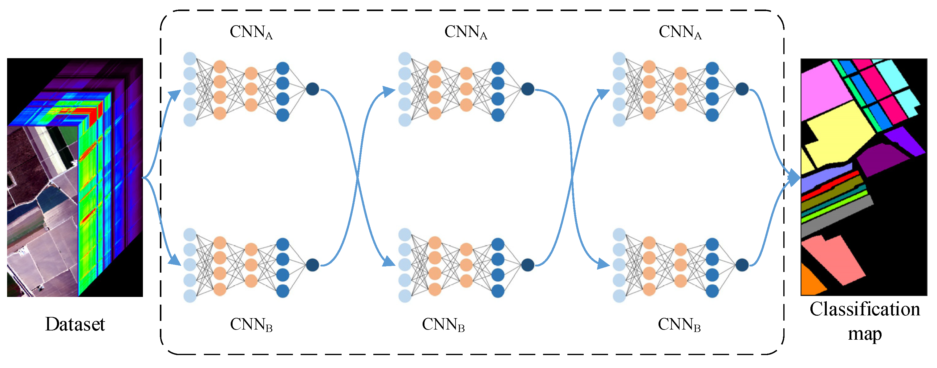
A new framework incorporating “disagreement” strategy into co-learning, named DCL, is proposed for HSI classification with noisy labels.

(2)

A stronger framework that introduces an “agreement” strategy into DCL, termed ADCL, is designed.

(3)

A joint loss function is proposed for the dual-network structure.

(4)

Extensive experiments on public HSI data sets demonstrate the effectiveness of the proposed method.

3. Proposed ADCL Method

The loss function is an essential component of deep neural networks, and a noise robust loss function can significantly improve their performance. In the proposed ADCL framework, two networks with the same structure are used, and a joint loss function is designed to make the framework more robust. The loss function takes into account the supervision information and the mutual guidance information between the two networks.

The main idea of ADCL is to have the two networks guide each other in learning. To achieve this goal, in the training process of ADCL, two networks predict all samples, and the samples with inconsistent predictions constitute the disagreement data. At the end of forward propagation, each deep network selects data with small loss from disagreement data to minimize the loss of the network. In the back propagation process, each network uses the data with small loss from the peer network to update the weight parameters. To make the model more powerful, in addition to selecting its own small loss data from disagreement data, each network also adds the data with the same classification on two networks into the peer network for back propagation. This design makes full use of the mutual information between the two networks, enhancing the noise tolerance of the model.

Taking CNN as the backbone for our ADCL, Figure 1 shows the overall framework of ADCL. Firstly, the training data with noisy labels is fed into two CNNs: $\mathrm{A}$ and $\mathrm{B}$. Secondly, after training one mini-batch, disagreement and consistent data predictions will be generated by the two networks. Thirdly, the two networks select their own small loss data according to the designed loss. Fourthly, each network uses the small loss data from the peer network and consistent data from two networks to update its own convolution kernels. Finally, after multiple epochs of training and updating, the two trained networks are combined to generate the classification map.

In the next subsections, we will introduce the designed joint loss, then detail the proposed ADCL framework, and finally show the formula analysis of the proposed method.

3.1. Joint Loss

In the case of the dual network, the most straightforward way to construct a loss function is to apply independent regularization when training each individual network. Although regularization can improve generalization performance by promoting consistency between two networks, it can still be influenced by the memory effect of label noise [35]. Therefore, we adopt a joint loss function based on regularization techniques in this work.

Let $T={\left\{x_i,y_i\right\}}_{i=1}^N$ be the training set with $N$ samples, where $x_i$ represents the ith sample, and its corresponding observation label is $y_i\in \left\{1,\dots ,C\right\}$. The joint loss function is designed as

$$l\left(x_i\right)=\beta l_S\left(x_i,y_i\right)+\left(1-\beta \right)l_R\left(x_i\right),$$

(1)

where $l_S$ represents the supervision loss under two networks, $l_R$ represents the relative loss, and parameter $\beta$ is utilized to balance the supervision loss and relative loss.

The symmetric cross-entropy (SCE) adds reverse cross-entropy (RCE) to cross-entropy (CE), so as to have a certain robustness to label noise [70]. This paper adopts SCE to construct supervision loss $l_S$. Before introducing SCE, the relationship between CE and Kullback–Leibler (KL) divergence is analyzed first, and then, the definition of SCE is introduced. Based on SCE, the supervision loss $l_S$ is constructed.

For each sample $x_i$, the class predictive distribution predicted by a classifier is denoted as $p(c|x_i)$, and $q\left(c|x_i\right)$ is used to represent the ground-truth distribution of the sample $x_i$ on the observation label. The CE loss is defined as

$$l_{ce}=-{\sum }_{c=1}^{C}q\left(c|x_i\right)\log p\left(c|x_i\right)=H\left(q,p\right),$$

(2)

when $c=y_i$, $q\left(c|x_i\right)=1$; otherwise, $q\left(c|x_i\right)=0$. The relationship between cross-entropy $H\left(q,p\right)$ and KL divergence can be written as

$$KL(q||p)=H\left(q,p\right)-H\left(q\right),$$

(3)

generally, $H\left(q\right)$ is a constant for a given ground-truth distribution, so it can be omitted from Formula (3) to obtain Formula (2). From the perspective of KL divergence, the essence of classification is to learn a prediction distribution $p\left(c|x_i\right)$ that is close to the ground-truth distribution $q\left(c|x_i\right)$, which minimizes the KL divergence between the two distributions. In the case of label noise, $q\left(c|x_i\right)$ as the ground-truth distribution, it does not represent a real class probability distribution. On the contrary,$p\left(c|x_i\right)$ to a certain extent reflects the true distribution. Therefore, in addition to $q\left(c|x_i\right)$ as a ground truth, we also need to consider the KL divergence in the other direction, namely $KL(p||q)$. Thus, the symmetric KL divergence is written as

$$SKL=KL(q||p)+KL(p||q).$$

(4)

According to the relationship between KL divergence and CE, the SCE and its corresponding loss can be written as follows:

$$SCE=CE+RCE=H\left(q,p\right)+H\left(p,q\right).$$

(5)

$$l_{sce}\left(x_i\right)=-{\sum }_{c=1}^{C}q\left(c|x_i\right)\log p\left(c|x_i\right)-{\sum }_{c=1}^{C}p\left(c|x_i\right)\log q\left(c|x_i\right).$$

(6)

For the two networks $\mathrm{A}$ and $\mathrm{B}$, the supervision loss $l_S$ constructed with SCE loss is defined as

$$l_S\left(x_i\right)=l_{sce}^A\left(x_i\right)+l_{sce}^B\left(x_i\right).$$

(7)

Generally speaking, the two networks can filter out the errors caused by noisy labels due to their different learning abilities, enabling the model to iterate forward stably. As can be seen from Formula (7), the supervision loss $l_S$ comes from the loss combinations under two networks, and each individual network uses SCE loss with good noise resistance, which enables $l_S$ to optimize the model in the right direction.

In addition to the supervision loss $l_S$ on the two networks allowing the model to be more stable, the relative loss $l_R$ between the two networks is also useful in identifying noisy labels. According to the principle of consistency maximization, different models will make an agreement on the correct labels for most samples, while it is unlikely to agree on the wrong labels. Suppose the predictive distributions of sample $x_i$ on two networks $\mathrm{A}$ and $\mathrm{B}$ are $p_A$ and $p_B$, respectively; we use R-Drop [71] to regularize the model predictions by minimizing the bidirectional KL divergence between these two predictive distributions for the sample $x_i$. The R-Drop-based relative loss is defined as

$$l_R\left(x_i\right)=\frac{1}{2}\left[D_{\mathrm{KL}}\left(p_A\parallel p_B\right)+D_{\mathrm{KL}}\left(p_B\parallel p_A\right)\right],$$

(8)

where $D_{\mathrm{KL}}\left(p_A\parallel p_B\right)={\sum }_{c=1}^C{p}_A^c\left(x_i\right)\log \frac{p_A^c\left(x_i\right)}{p_B^c\left(x_i\right)}$, $D_{\mathrm{KL}}\left(p_B\parallel p_A\right)={\sum }_{c=1}^C{p}_B^c\left(x_i\right)\log \frac{p_B^c\left(x_i\right)}{p_A^c\left(x_i\right)}$. It can be seen from Formula (8) that the relative loss between the two networks is paired, and the relative loss is only related to the predictive distributions. The relative loss reflects the degree of consistency discrimination of two networks for the same sample.

Through the above analysis, the supervision loss and relative loss are obtained by Formulas (7) and (8), respectively. To this end, the joint loss induced by Formula (1) can be written as

$$l\left(x_i\right)=\beta \left[l_{sce}^A\left(x_i\right)+l_{sce}^B\left(x_i\right)\right]+\frac{\left(1-\beta \right)}{2}\left[D_{\mathrm{KL}}\left(p_A\parallel p_B\right)+D_{\mathrm{KL}}\left(p_B\parallel p_A\right)\right].$$

(9)

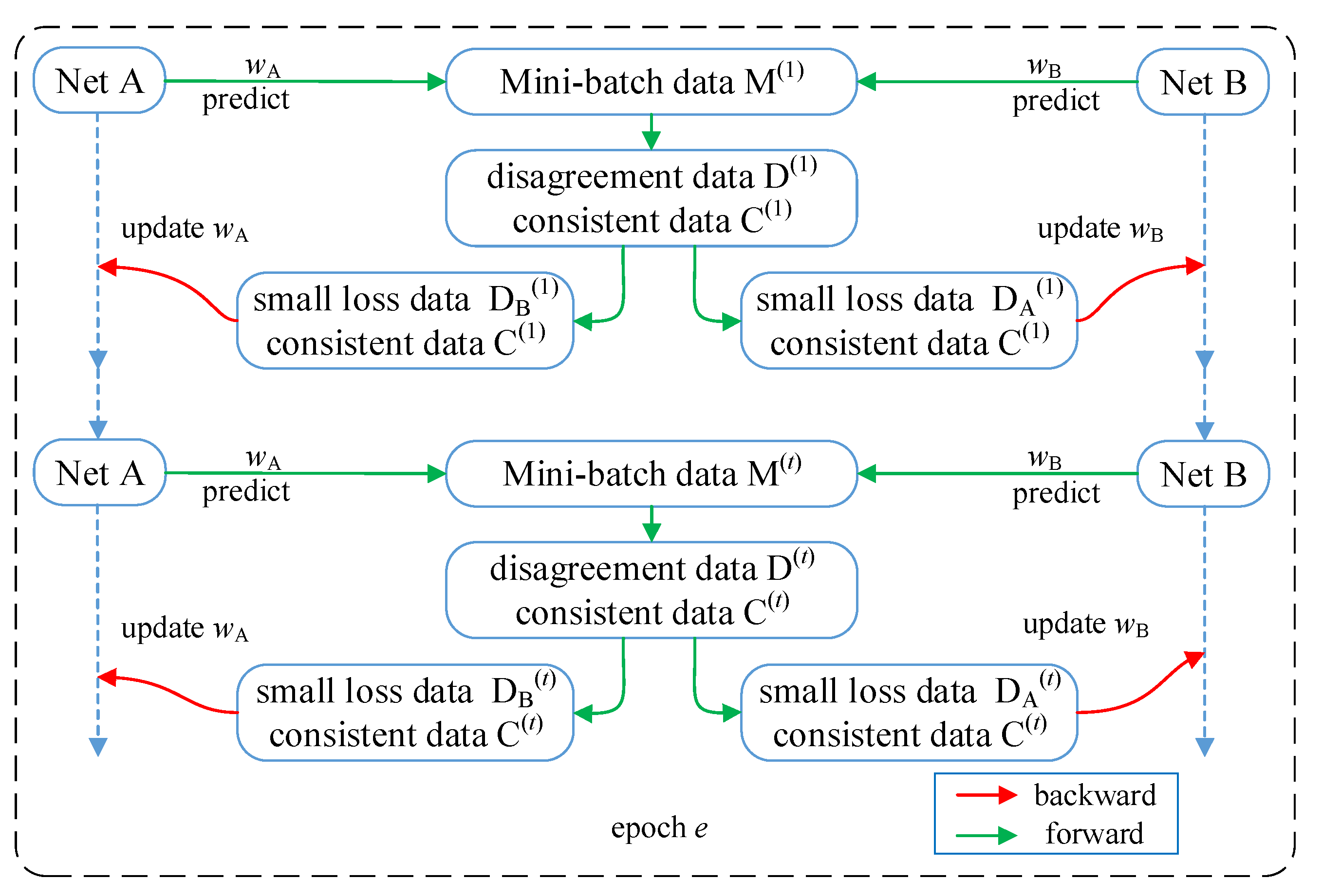
3.2. Agreement and Disagreement-Based Co-Learning Framework

Different learners utilize their own unique structures to learn decision boundaries and thus enjoy distinct learning abilities. Therefore, they are desired to exhibit distinct abilities to filter label noise when learning data with noisy labels. In this work, we propose an HSI classification method based on co-learning with a dual network, so that two networks can exchange and select samples with small losses, that is, update network A (corresponding to B) with mini-batch data selected from B (corresponding to A). If the selected sample is not completely “clean”, the two networks adapt to correct the peer-to-peer training errors. This is similar to cross-validation; since errors from one network are not propagated directly back to itself, it can be expected that the method based on co-learning with a dual network can handle higher noise.

As the number of iterations increases, the two networks reach an agreement, and the co-learning function decays into two self-training networks. To make the learning more robust, we incorporate “disagreement” strategy into the co-learning and put forward a more robust learning paradigm, namely, disagreement-based co-learning (DCL). The training process of DCL includes two update steps: data update and parameter update. First, in the data update stage, the two deep networks predict all samples in mini-batch and retain the data with inconsistent prediction results of the two deep networks, which maintains the divergence of two deep networks trained by the DCL. Then, in the parameter update stage, each deep network chooses data with small loss from the disagreement data to minimize the loss of the deep network and utilize the data with small loss from the peer network to update its own weight parameters. However, the “disagreement” strategy cannot guarantee real supervision information. Therefore, we leverage the “agreement” strategy in co-training to improve the DCL and propose an agreement and disagreement-based co-learning (ADCL) framework for HSI classification. During the parameter update of ADCL, each network selects its own small loss data from the disagreement data and adds the data with the same classification results of the two networks into the peer network for back propagation.

Figure 2 shows detailed procedure of forward propagation and back propagation. For the t-th mini-batch, the two networks $\mathrm{A}$ and $\mathrm{B}$ predict the mini-batch according to the parameters $w_{\mathrm{A}}$ and $w_{\mathrm{B}}$, respectively. The disagreement data ${\mathrm{D}}^{\left(t\right)}$ are determined by Formula (10), i.e., the samples with inconsistent predictions from the two networks.

$${\mathrm{D}}^{\left(t\right)}=\left\{\left(\left(x_i,y_i\right)\right):y_i^{\mathrm{A}}\ne y_i^{\mathrm{B}}\right\},$$

(10)

In the end of forward propagation, ${\mathrm{D}}_{\mathrm{A}}^{\left(t\right)}$ and ${\mathrm{D}}_{\mathrm{B}}^{\left(t\right)}$ are determined by Formula (11) so that the losses of network $\mathrm{A}$ and $\mathrm{B}$ are minimized.

$$\left\{\begin{array}{c}{\mathrm{D}}_{\mathrm{A}}^{\left(t\right)}=\arg mi{n}_{{\mathrm{D}}_{\mathrm{A}}:\left|{\mathrm{D}}_{\mathrm{A}}\right|\ge \lambda \left(e\right)\left|{\mathrm{D}}^{\left(t\right)}\right|}l\left({\mathrm{D}}_{\mathrm{A}},w_{\mathrm{A}}\right)\\ {\mathrm{D}}_{\mathrm{B}}^{\left(t\right)}=\arg mi{n}_{{\mathrm{D}}_{\mathrm{B}}:\left|{\mathrm{D}}_{\mathrm{B}}\right|\ge \lambda \left(e\right)\left|{\mathrm{D}}^{\left(t\right)}\right|}l\left({\mathrm{D}}_{\mathrm{B}},w_{\mathrm{B}}\right)\end{array}\right.,$$

(11)

where $\lambda \left(e\right)$ is used to control how much small loss data should be chosen in every $epoch\left(e\right)$. Because of the memory effect, the deep network will first match data without noise and then gradually fit data with label noise. Formula (12) relates the noise rate $r$ and the parameter $\lambda \left(e\right)$, which controls the amount of small loss data to be chosen in each epoch.

$$\lambda \left(e\right)=1-\left(1+\frac{e-E_k}{E_{max}-E_k}\right)r,$$

(12)

where $E_k$ and $E_{max}$ represent a constant and the biggest $epoch$ value, respectively. As can be seen from Formula (12), $\lambda \left(e\right)$ is large at the beginning of the training phase, which would maintain more data with small loss. As the $epoch$ increase, less data with small loss are retained in each mini-batch. The gradual decrease in $\lambda \left(e\right)$ alleviates the overfitting on noisy data of deep networks to a great extent.

$$\left\{\begin{array}{c}{w}_{\mathrm{A}}=w_{\mathrm{A}}-\eta \nabla l\left({\mathrm{D}}_{\mathrm{B}}^{\left(t\right)}+{\mathrm{C}}^{\left(t\right)},w_{\mathrm{A}}\right)\\ w_{\mathrm{B}}=w_{\mathrm{B}}-\eta \nabla l\left({\mathrm{D}}_{\mathrm{A}}^{\left(t\right)}+{\mathrm{C}}^{\left(t\right)},w_{\mathrm{B}}\right)\end{array}\right.,$$

(13)

In back propagation, we use Formula (13) to update the network weight parameters, which can ensure that there are real distributions playing a role in the training under the condition of high noise rate. It can be seen that when updating the weight parameters of networks $\mathrm{A}$ and $\mathrm{B}$, not only the disagreement data are used, but also the consistent data are added to calculate the loss. The consistent data ${\mathrm{C}}^{\left(t\right)}$ in Formula (13) can be obtained by Formula (14).

$${\mathrm{C}}^{\left(t\right)}=\left\{\left(\left(x_i,y_i\right)\right):y_i^{\mathrm{A}}=y_i,y_i^{\mathrm{B}}=y_i\right\}.$$

(14)

3.3. Formula Analysis

In this subsection, we use formulas to analyze the main procedure of the proposed method. We use the 2D convolutional neural network as the backbone to describe the method.

The symbols A and B represent two convolutional neural networks with initial convolutional kernels w_A and w_B, l represents the l-th layer, and δ means the gradient. Suppose that the data are divided into m mini-batch. For the i-th mini-batch data D, the training process can be described as follows:

Forward Propagation:

1. Assign the input data $x$ to the input neurons $a_A^1$ and $a_B^1$, $a_A^1=x$, $a_B^1=x$.

2. For the second layer to the $L-1$ layer, perform forward propagation calculations according to the following three cases:

2.1. If the current layer is a convolutional layer, then we have $a_A^l=\sigma \left(z_A^l\right)=\sigma \left(w_A*a_A^{l-1}+b_A^l\right)$, $a_B^l=\sigma \left(z_B^l\right)=\sigma \left(w_B*a_B^{l-1}+b_B^l\right)$.

2.2. If the current layer is a pooling layer, then we have $a_A^l=pooling\left(a_A^{l-1}\right)$, $a_B^l=pooling\left(a_B^{l-1}\right)$.

2.3. If the current layer is a fully connected layer, then we have $a_A^l=\sigma \left(z_A^l\right)=\sigma \left(w_A{a}_A^{l-1}+b_A^l\right)$, $a_B^l=\sigma \left(z_B^l\right)=\sigma \left(w_B{a}_B^{l-1}+b_B^l\right)$.

3. Output layer: $a_A^L=softmax\left(z_A^L\right)=softmax\left(w_A{a}_A^{L-1}+b_A^L\right)$, $a_B^L=softmax\left(z_B^L\right)=softmax\left(w_B{a}_B^{L-1}+b_B^L\right)$.

4. Obtain the small loss data ${\mathrm{D}}_A$ and ${\mathrm{D}}_B$ through Formula (11). Obtain the consistent data $\mathrm{C}$ by Formula (14).

Back Propagation:

1. Compute the gradient of output layer ${\delta }_A^L\left({\mathrm{D}}_B+\mathrm{C}\right)$ and ${\delta }_B^L\left({\mathrm{D}}_A+\mathrm{C}\right)$.

2. For the $L-1$ layer to the second layer, perform backward propagation according to the following three cases:

2.1. If the current layer is a fully connected layer, then we have ${\delta }_A^l={\left(w_A^{l+1}\right)}^T{\delta }_A^{l+1}\left({\mathrm{D}}_B+\mathrm{C}\right)\oplus {\sigma }^{\prime }\left(z_A^l\left({\mathrm{D}}_B+\mathrm{C}\right)\right)$, ${\delta }_B^l={\left(w_B^{l+1}\right)}^T{\delta }_B^{l+1}\left({\mathrm{D}}_A+\mathrm{C}\right)\odot {\sigma }^{\prime }\left(z_B^l\left({\mathrm{D}}_A+\mathrm{C}\right)\right)$.

2.2. If the previous layer is a pooling layer, then we have ${\delta }_A^l=upsampling\left({\delta }_A^{l+1}\left({\mathrm{D}}_B+\mathrm{C}\right)\right)$, ${\delta }_B^l=upsampling\left({\delta }_B^{l+1}\left({\mathrm{D}}_A+\mathrm{C}\right)\right)$.

2.3. If previous layer is a convolutional layer, then we have ${\delta }_A^l={\delta }_A^{l+1}*rot180\left(w_A^{l+1}\right)\odot {\sigma }^{\prime }\left(z_A^l\left({\mathrm{D}}_B+\mathrm{C}\right)\right)$, ${\delta }_B^l={\delta }_B^{l+1}*rot180\left(w_B^{l+1}\right)\odot {\sigma }^{\prime }\left(z_B^l\left({\mathrm{D}}_A+\mathrm{C}\right)\right)$.

3. Then, we can update the model parameters:

3.1. If the current layer is a fully connected layer, we have $w_A^l=w_A^l-\frac{\eta }{m}\sum {\delta }_A^l{\left(a_{{\mathrm{D}}_B+\mathrm{C}}^{l-1}\right)}^T$, $w_B^l=w_B^l-\frac{\eta }{m}\sum {\delta }_B^l{\left(a_{{\mathrm{D}}_A+\mathrm{C}}^{l-1}\right)}^T$.

3.2. If the current layer is the convolutional layer, we have $w_A^l=w_A^l-\frac{\eta }{m}\left[\sum {\delta }_B^l*rot90\left(a_{{\mathrm{D}}_B+\mathrm{C}}^{l-1},2\right)\right]$, $w_A^l=w_A^l-\frac{\eta }{m}\left[\sum {\delta }_A^l*rot90\left(a_{{\mathrm{D}}_A+\mathrm{C}}^{l-1},2\right)\right]$.

The above description is the main steps of the proposed method. It can be seen that the dual-network structure uses the information of the peer network to guide each other in the training process, and the network structure is easy to implement.

4. Experimental Results and Analysis

4.1. HSI Data Sets

To demonstrate the effectiveness of our proposed method, we conducted experiments on three publicly available HSI data sets. The detailed descriptions of the three data sets are provided below:

(1)

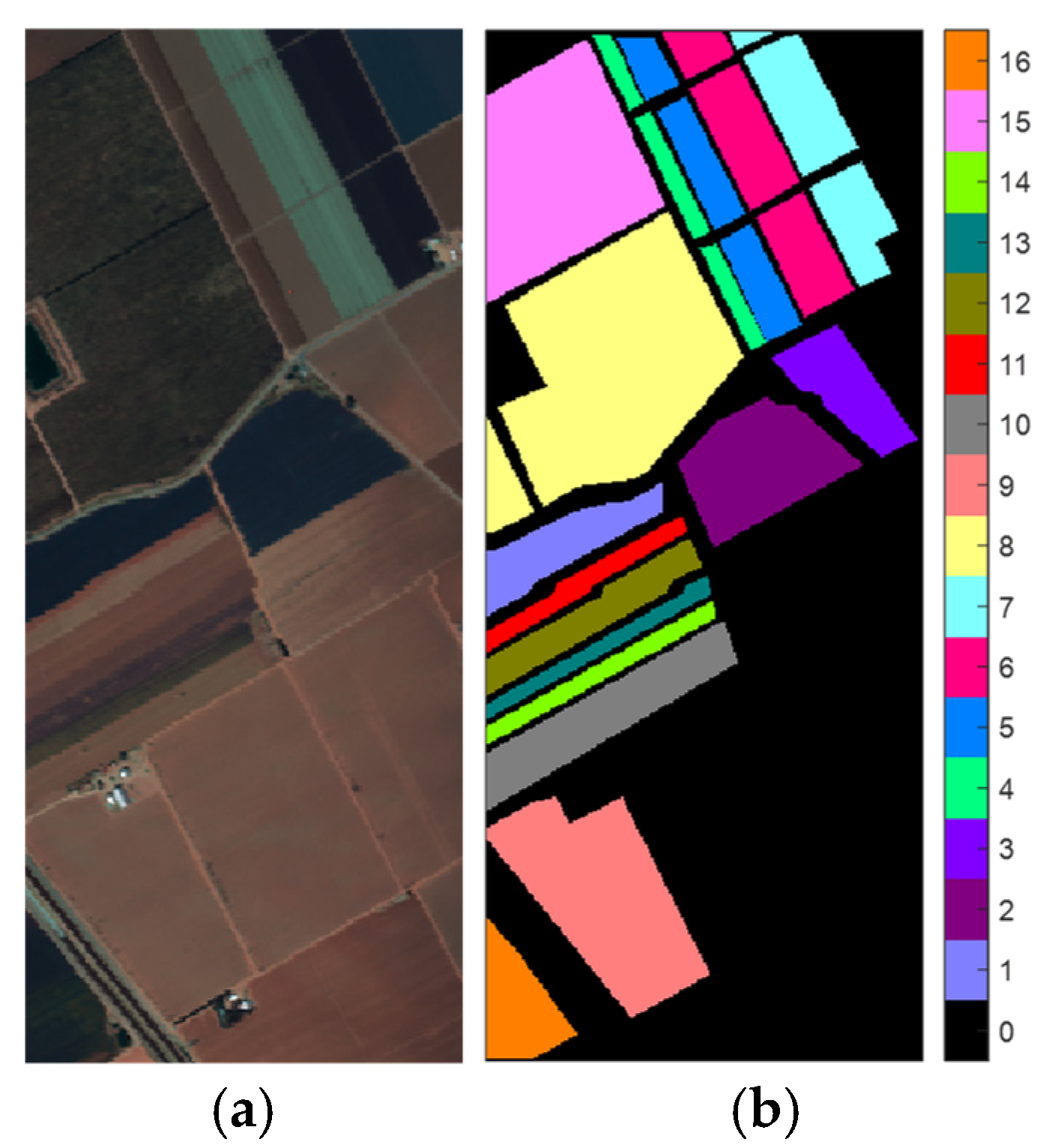
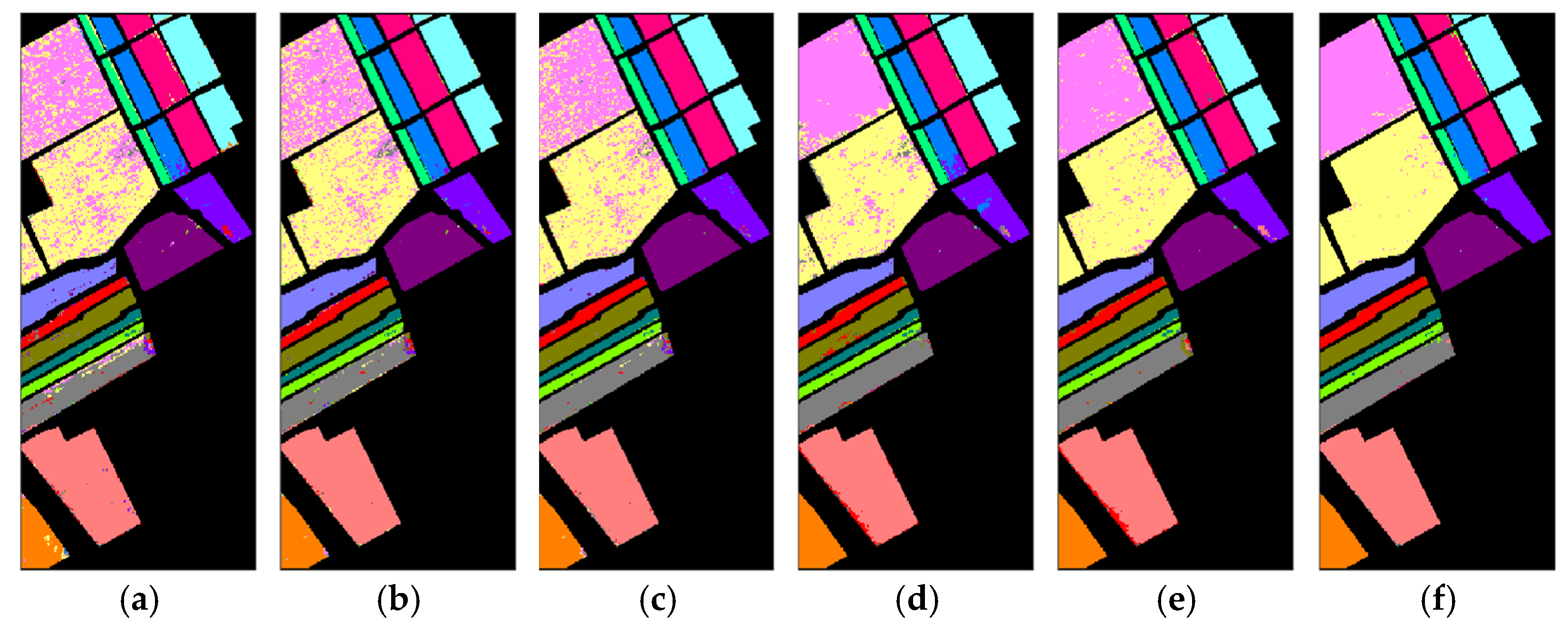
Salinas Valley (SV) [72]: The SV data set was collected by the Airborne Visible/Infrared Imaging Spectrometer (AVIRIS) sensor over the agricultural area described as Salinas Valley in California, USA, in 1998. The data set contains 512 × 217 pixels characterized by 224 spectral bands. A total of 204 bands were used for experiments after removing 20 redundant ones. The spatial resolution of SV is 3.7 m per pixel, and the land cover contains 16 classes. The three-band pseudocolor image of the SV and its corresponding reference map are illustrated in Figure 3.

(2)

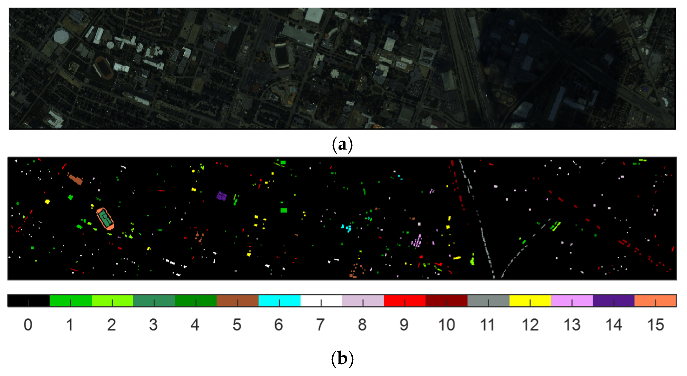
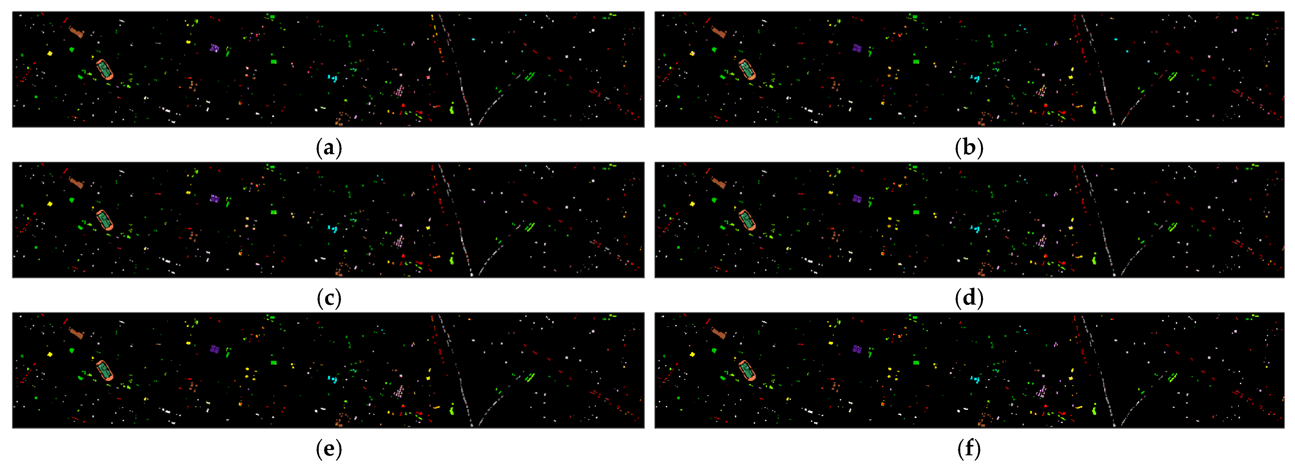
Houston (HOU) [73]: The HOU data set was obtained by the ITRES CASI-1500 sensor and provided by the 2013 IEEE GRSS Data Fusion Competition. The data set contains 349 × 1905 pixels characterized by 144 spectral bands ranging from 364 to 1046 nm. The spatial resolution of HOU is 2.5 m per pixel, and the land cover includes 15 classes. The three-band pseudocolor image of the HOU and its corresponding reference map are shown in Figure 4.

(3)

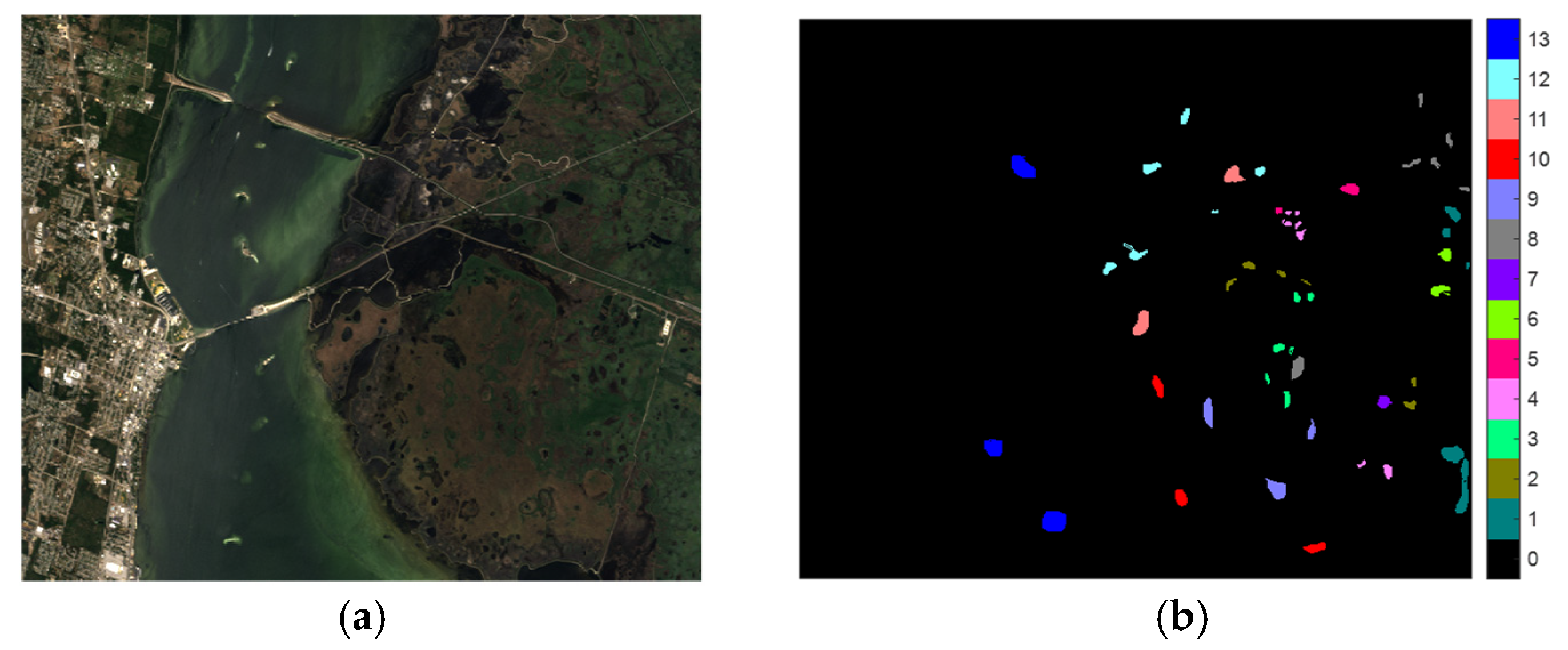
Kennedy Space Center (KSC) [72]: The KSC data set was acquired by the AVIRIS sensor over the KSC, Florida, on 23 March 1996. The data set contains 512 × 614 pixels characterized by 224 spectral bands. A total of 176 bands were retained for our experiment after removing water absorption bands and low signal-to-noise ratio bands. The spatial resolution of KSC is 3.7 m per pixel, and the land cover includes 13 classes. The three-band pseudocolor image of the KSC and its corresponding reference map are illustrated in Figure 5.

For each data set, we randomly selected 10% of the samples as the training set, and the remaining 90% of the samples were treated as the testing set. Detailed descriptions of the three HIS data sets are given in

Table 1. The class information and data partition of SV data set.

Class No.	Class Name	Train	Test	Total
1	Brocoli_green_weeds_1	201	1808	2009
2	Brocoli_green_weeds_2	373	3353	3726
3	Fallow	198	1778	1976
4	Fallow_rough_plow	139	1255	1394
5	Fallow_smooth	268	2410	2678
6	Stubble	396	3563	3959
7	Celery	358	3221	3579
8	Grapes_untrained	1127	10144	11271
9	Soil_vinyard_develop	620	5583	6203
10	Corn_senesced_green_weeds	328	2950	3278
11	Lettuce_romaine_4wk	107	961	1068
12	Lettuce_romaine_5wk	193	1734	1927
13	Lettuce_romaine_6wk	92	824	916
14	Lettuce_romaine_7wk	107	963	1070
15	Vinyard_untrained	727	6541	7268
16	Vinyard_vertical_trellis	181	1626	1807

,

Table 2. The class information and data partition of HOU data set.

Class No.	Class Name	Train	Test	Total
1	Healthy grass	125	1126	1251
2	Stressed grass	125	1129	1254
3	Stressed grass	70	627	697
4	Trees	124	1120	1244
5	Soil	124	1118	1242
6	Water	33	292	325
7	Residential	127	1141	1268
8	Commercial	124	1120	1244
9	Road	125	1127	1252
10	Highway	123	1104	1227
11	Railway	124	1111	1235
12	Parking Lot 1	123	1110	1233
13	Parking Lot 2	47	422	469
14	Tennis Court	43	385	428
15	Running Track	66	594	660

and

Table 3. The class information and data partition of KSC data set.

Class No.	Class Name	Train	Test	Total
1	Scrub	76	685	761
2	Willow swamp	24	219	243
3	Cabbage palm hammock	26	230	256
4	Cabbage palm/oak hammock	25	227	252
5	Slash pine	16	145	161
6	Oak/broadleafhammock	23	206	229
7	Hardwood swamp	11	94	105
8	Graminoid marsh	43	388	431
9	Spartina marsh	52	468	520
10	Cattail marsh	40	364	404
11	Salt marsh	42	377	419
12	Mud flats	50	453	503
13	Water	93	834	927

.

4.2. Experiment Settings

In our experiments, we used a 2D CNN as the backbone to implement our ADCL. For simplicity, we denoted the 2D CNN-based ADCL as 2D-ADCL. In 2D-ADCL, the Adam optimizer was adopted to dominate the training process. We set the learning rate to 0.001 with 150 epochs. We implemented 2D-ADCL in PyTorch 1.8.1, and a single NVIDIA RTX 3070 GPU with CUDA 11.1 was used to boost the training process.

To generate training sets with different label noise levels, we randomly selected a portion of samples from the training set and uniformly assigned any other class labels to them. We set different noise ratios $r$ to obtain training sets with different levels of label noise. We used several metrics, including overall accuracy (OA), average accuracy (AA), and Kappa coefficient (k), to evaluate the classification performance of the proposed method. Detailed calculations of these metrics are given below.

The overall accuracy can be calculated by Formula (15).

$$\mathrm{OA}=\frac{{\sum }_{i=1}^C{M}_i}{M},$$

(15)

where C represents the number of class, and $M_i$ represents the number of correctly classified samples in the i-th class.

The calculation of average accuracy is shown in Formula (16).

$$\mathrm{AA}=\frac{{\sum }_{i=1}^C{\mathrm{UA}}_i}{C},$$

(16)

where ${\mathrm{UA}}_i=M_{ii}/{\sum }_{j=1}^C{M}_{ij}$ is the ratio of the number of correctly classified samples in the i-th class to the total number of samples in the i-th class, and $M_{ij}$ represents the number of samples of the i-th class that are classified as the j-th class.

The kappa coefficient can be obtained by Formula (17).

$$\mathrm{Kappa}=\frac{N{\sum }_{i=1}^C{M}_{ii}-{\sum }_{i=1}^C\left({\sum }_{j=1}^C{M}_{ij}{\sum }_{j=1}^C{M}_{ji}\right)}{N^2-{\sum }_{i=1}^C\left({\sum }_{j=1}^C{M}_{ij}{\sum }_{j=1}^C{M}_{ji}\right)},$$

(17)

4.3. Evaluation of the Joint Loss Function

To evaluate the performance of the designed joint loss function, we set the noise ratio $r$ to 0.3 for the experiments, i.e., 30% of training samples were randomly assigned with wrong labels. The proposed joint loss function has a parameter $\beta$ that is used to balance the supervision loss and relative loss in the joint loss. We conducted experiments with different values of $\beta$ varying from 0.05 to 0.95 with a step of 0.05. The OA curves of 2D-ADCL on the three HSI data sets were illustrated in Figure 6. As can be seen from Figure 6, a relatively small $\beta$ can obtain better performance than a large $\beta$, which means that the relative loss should obtain more attention.

The designed loss is related to CE loss, SCE loss, and R-Drop loss. We compared the proposed joint loss with CE loss, SCE loss and R-Drop loss on three HSI data sets, where $\beta$ was set to 0.15 for the proposed joint loss. The classification accuracies of 2D-ADCL with different loss functions on the three data sets are shown in

Table 4. Classification accuracy of different loss functions on three data sets. The comparison loss functions include CE, SCE, and R-Drop. The Oas, Aas, and kappas of different methods are reported.

Data Sets	SV				HOU				KSC
Loss	CE	SCE	R-Drop	Proposed	CE	SCE	R-Drop	Proposed	CE	SCE	R-Drop	Proposed
OA	93.21	95.26	95.38	98.62	84.75	86.35	87.11	90.89	95.58	97.28	97.45	99.02
AA	92.35	95.14	95.78	98.73	84.54	85.92	86.87	90.94	95.43	96.87	97.14	98.50
k × 100	91.95	95.08	95.46	98.47	84.39	86.11	86.94	90.11	95.17	97.05	97.23	98.91

. The results in Table 4 demonstrate that the proposed joint loss obtains the best performance, R-Drop loss achieves suboptimal performance, and the other two loss functions perform less well.

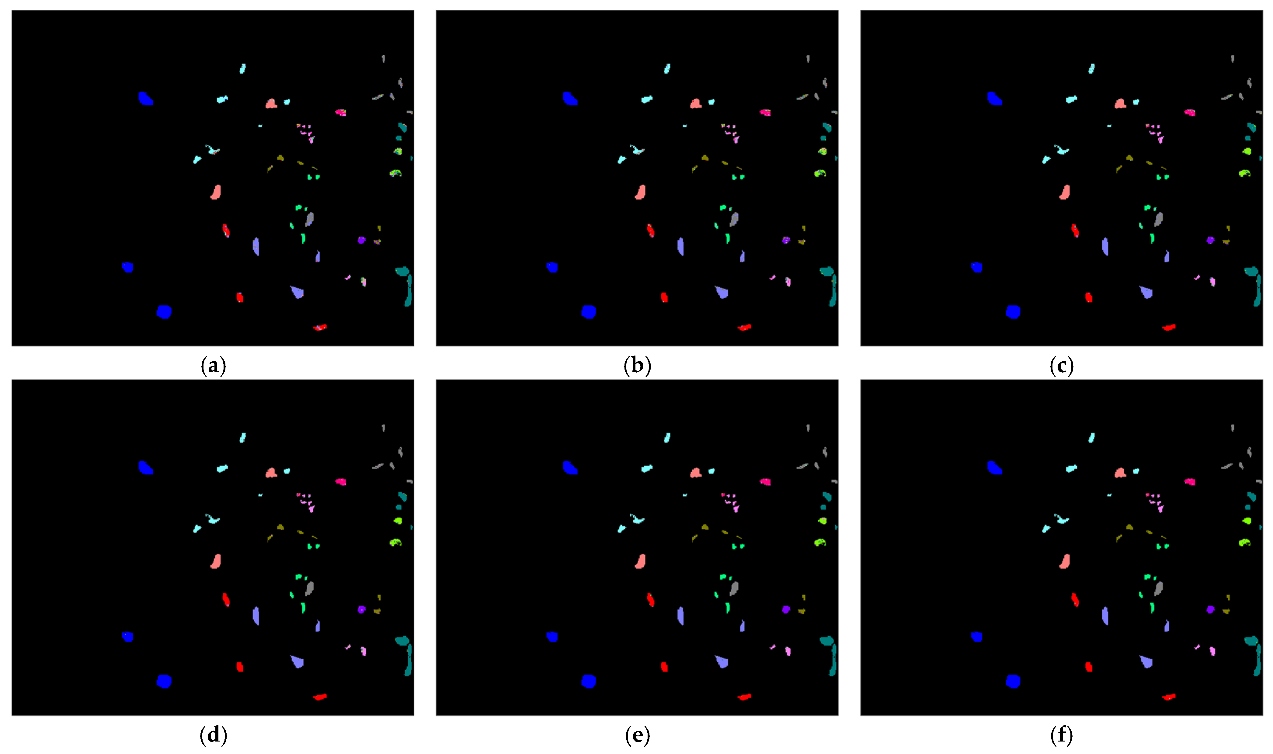
4.4. Comparison with State-of-the-Art Methods

We compared 2D-ADCL with state-of-the-art methods to demonstrate its performance. The comparison methods include RLPA [15], DPNLD [12], SALP [17], DCRN [20], and S3Net [21]. The detailed settings for the above methods were consistent with their corresponding references. It should be noted that the SVM classifier was used as the base classifier for RLPA, DPNLD, and SALP, while 2D-CNN was adopted as the backbone network for S3Net. The noise rate $r$ was set to 0.3. We repeated each algorithm ten times to obtain the average results.

Table 5. Classification accuracy (in %) including class-specific accuracy, OA, AA, and kappa on SV data set. Classification accuracy obtained by RLPA, DPNLD, SALP, DCRN, S3Net, and 2D-ADCL with 30% noisy labels in the training set.

Class	RLPA [15]	DPNLD [12]	SALP [17]	DCRN [20]	S3Net [21]	2D-ADCL
1	97.75	98.48	99.83	99.70	99.50	99.99
2	99.14	99.75	99.80	99.78	99.35	99.86
3	96.56	97.07	99.55	92.73	98.31	99.78
4	89.88	99.69	99.53	99.64	99.64	98.86
5	94.28	96.84	96.61	88.23	96.73	97.18
6	97.47	98.74	97.83	98.94	94.54	97.19
7	98.11	99.20	99.44	99.78	99.80	99.80
8	72.88	79.39	78.50	88.45	94.06	98.20
9	97.35	99.02	98.79	95.32	94.28	99.43
10	78.91	87.22	92.60	96.33	93.28	97.19
11	90.94	91.84	96.81	96.03	95.35	98.34
12	97.43	99.62	99.02	94.62	91.53	99.89
13	97.32	97.43	98.33	97.46	98.88	98.52
14	93.17	94.95	94.17	93.30	96.11	97.36
15	74.99	69.92	77.71	91.76	96.69	98.03
16	94.15	98.30	98.59	99.98	99.39	100
OA	87.77	90.01	91.16	94.31	96.04	98.62
AA	91.90	94.22	94.58	95.76	96.72	98.73
k × 100	86.41	88.87	90.17	93.68	95.59	98.47

,

Table 6. Classification accuracy (in %) including class-specific accuracy, OA, AA, and kappa on HOU data set. Classification accuracy obtained by RLPA, DPNLD, SALP, DCRN, S3Net, and 2D-ADCL with 30% noisy labels in the training set.

Class	RLPA [15]	DPNLD [12]	SALP [17]	DCRN [20]	S3Net [21]	2D-ADCL
1	90.21	93.47	90.66	95.09	95.16	98.05
2	96.99	98.53	91.78	98.54	97.68	98.83
3	92.67	88.42	97.77	98.02	97.24	97.69
4	91.72	92.46	91.80	96.27	96.85	97.16
5	93.76	95.80	95.40	96.53	98.09	98.12
6	83.65	94.44	92.47	95.29	91.59	98.59
7	82.92	76.63	80.75	84.47	85.50	92.22
8	68.36	63.92	68.68	78.68	82.20	86.47
9	73.19	79.95	77.81	77.19	84.87	83.25
10	71.76	78.33	74.35	87.71	85.29	89.84
11	68.79	58.30	70.19	78.18	84.74	81.70
12	27.79	45.45	58.08	71.90	81.59	79.11
13	25.88	23.16	38.30	44.73	36.57	66.27
14	92.05	96.10	89.37	97.62	98.13	98.35
15	82.76	95.16	97.60	96.85	95.55	98.32
OA	76.63	78.69	80.86	86.67	88.62	90.89
AA	76.17	78.68	81.00	86.47	87.40	90.94
k × 100	74.74	76.95	79.30	85.56	87.69	90.11

and

Table 7. Classification accuracy (%) including class-specific accuracy, OA, AA, and kappa on KSC data set. Classification accuracy obtained by RLPA, DPNLD, SALP, DCRN, S3Net, and 2D-ADCL with 30% noisy labels in the training set.

Class	RLPA [15]	DPNLD [12]	SALP [17]	DCRN [20]	S3Net [21]	2D-ADCL
1	97.50	96.98	97.90	98.82	99.47	99.21
2	84.77	91.77	93.42	95.47	97.94	97.94
3	90.33	90.23	94.14	96.88	97.66	100
4	70.24	76.98	87.30	88.10	94.44	97.62
5	59.63	65.22	77.02	86.90	91.30	93.79
6	51.97	64.63	80.35	95.24	88.65	94.76
7	92.38	74.29	95.24	99.07	100	100
8	84.69	90.22	95.13	98.85	98.61	98.84
9	91.92	93.46	97.50	99.01	99.04	99.81
10	86.14	95.43	96.78	98.97	97.77	99.01
11	97.18	98.57	99.28	99.05	99.69	99.76
12	90.66	93.84	96.82	98.41	99.81	99.80
13	99.75	99.76	99.89	99.89	100	100
OA	89.20	91.86	95.53	97.35	98.16	99.02
AA	84.40	87.01	93.14	95.73	97.19	98.50
k × 100	87.95	90.93	95.02	97.05	97.95	98.91

show the OAs, Aas, kappa coefficients, and class-specific accuracies of the comparison methods on the SV, HOU, and KSC data sets, respectively. The best classification accuracies of different methods are highlighted in bold. The classification result maps of different methods on the SV, HOU, and KSC data sets are illustrated in Figure 7, Figure 8 and Figure 9, respectively.

Several results can be observed from Table 5, Table 6 and Table 7 and Figure 7, Figure 8 and Figure 9. Firstly, 2D-ADCL achieves higher class-specific accuracy than other methods in most cases. Specifically, 2D-ADCL attains 13, 11, and 10 best class-specific accuracies on SV, BOT, and KSC data sets, respectively. Secondly, 2D-ADCL achieves the best OAs, AAs, and kappa coefficients on all data sets. The average OA of 2D-ADCL is more than two percentage points higher than the second-place and more than 10 percentage points higher than the last place. Thirdly, the accuracies of deep learning-based methods (DCRN, S3Net, and 2D-ADCL) are significantly higher than those of traditional methods (RLPA, DPNLD, and SALP). Fourthly, the classification maps of different methods on the three data sets demonstrate that 2D-ADCL achieves satisfactory classification results.

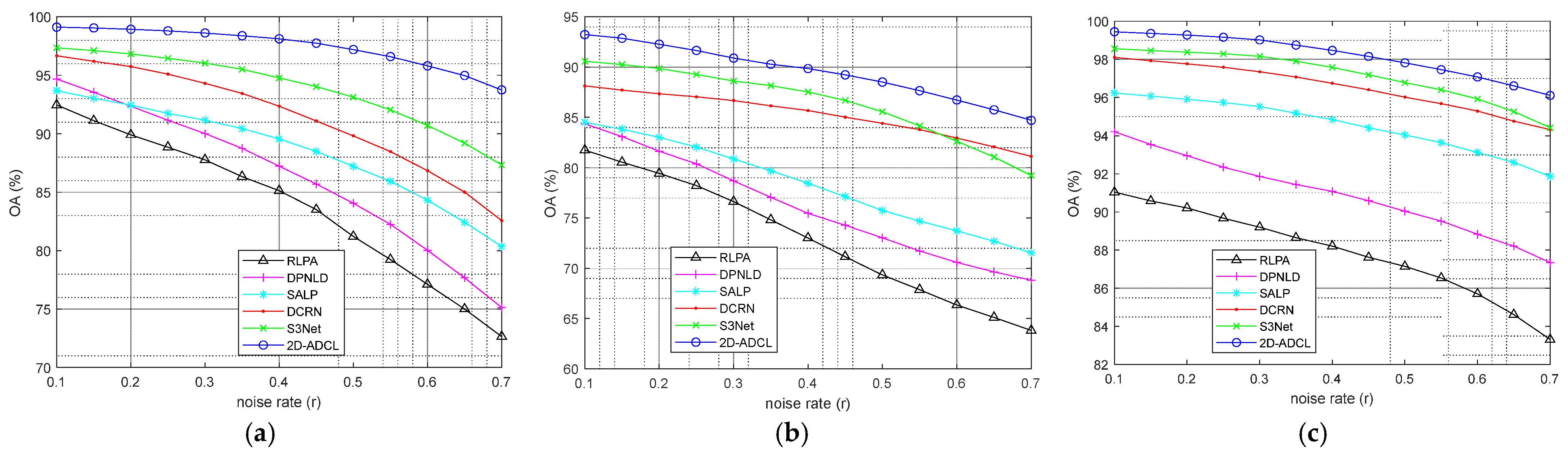
4.5. Performance Evaluation under Different Noise Rates

In order to study the effect of noise rate on classification performance, we set different noise rates for experiments, in which the noise rate ranged from 0.1 to 0.7 with a step of 0.05. First, when the noise rate was equal to 0.1, the training set contained only 10% of noisy samples. Then, the number of noisy samples in the training set increased gradually with the increase in noise rate. Finally, when the noise rate was equal to 0.7, the number of noisy samples in the training set reached 70%. We ran all methods ten times to obtain average results. The OA curves of different methods on SV, HOU, and KSC data sets are plotted in Figure 10.

As seen from Figure 10, for each data set, the classification result of 2D-ADCL is consistently better than that of the other methods in terms of OA. The average OA of all comparison methods decreases with the increase in noise rate. It can be seen that the deep learning-based methods (DCRN, S3Net, and 2D-ADCL) show a lower attenuation speed on OA than the traditional methods (RLPA, DPNLD, and SALP). When the noise rate increases from 0.1 to 0.7, the OA attenuation values of 2D-ADCL on SV, HOU, and KSC data sets are approximately within 5%, 8% and 4%, respectively. This indicates that ADCL is robust to high noise rates.

4.6. Computational Cost

Computational cost is also an important metric to evaluate classification algorithms. We set the noise rate to 0.5 to compare the running times of different methods, including training time and test time.

Table 8. Running times (s) on three data sets. Running time for RLPA, DPNLD, SALP, DCRN, S3Net, and 2D-ADCL, where the running time consists of training time and testing time.

Time (s)	SV	HOU	KSC
RLPA [15]	85.8	55.3	19.5
DPNLD [12]	65.5	41.3	26.5
SALP [17]	113.6	46.5	28.5
DCRN [20]	148.8	91.4	45.3
S3Net [21]	161.7	116.8	48.7
2D-ADCL	178.1	130.4	55.4

displays the running times of different methods on SV, HOU, and KSC data sets.

The results from Table 8 show that the running times for comparison methods range from tens of seconds to hundreds of seconds, and none of them require too much running time. Another finding is that the running times of deep learning-based methods are longer than those of traditional methods, since deep learning methods need more time for training models. For the three deep learning methods (DCRN, S3Net, 2D-ADCL), the running time of 2D-ADCL is slightly longer than that of the other two methods, which is still within the acceptable range.

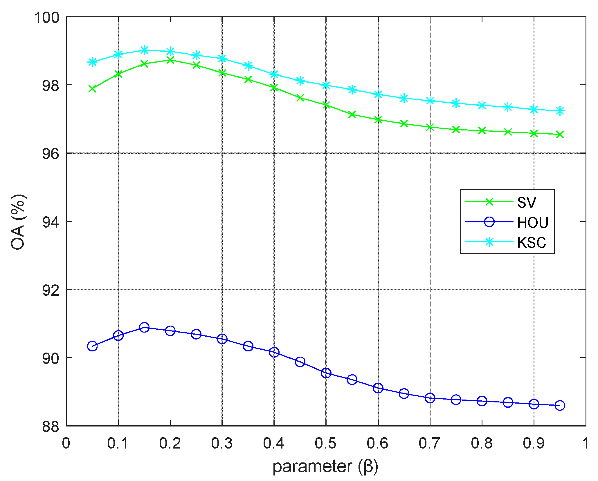
4.7. Further Analysis

In order to investigate the role of the “agreement” strategy in ADCL, we took ADCL and DCL for comparison, where DCL only adopted the data with a small loss from the peer network to update the weight parameters. The other settings for DCL are the same as ADCL.

Table 9. Classification results in terms of OA, AA, and kappa on three data sets. Classification accuracy obtained by 2D-DCL and 2D-ADCL with 50% noisy labels in the training set.

Data Sets	SV		HOU		KSC
Method	2D-DCL	2D-ADCL	2D-DCL	2D-ADCL	2D-DCL	2D-ADCL
OA	95.64	97.20	86.15	88.51	96.25	97.82
AA	95.82	97.34	86.44	88.43	95.74	97.14
k × 100	95.23	97.11	86.29	88.31	95.82	97.25

shows the classification results of the two methods when the noise rate was 0.5.

As seen from the results in Table 9, the average OAs, AAs, and kappa coefficients of 2D-ADCL on the three data sets are higher than those of 2D-DCL, indicating that the “agreement” strategy plays an important role in learning from label noise.

5. Discussion

Previous experiments revealed some important findings that require further discussion.

As demonstrated in Section 4.3, compared with related loss functions, the proposed joint loss function has better performance because it makes full use of both networks’ own supervision information and mutual information between the two networks. Additionally, the experimental results illustrate that the relative loss in the joint loss plays a more important role, because the supervision information from the peer network is more effective than its own supervision information in the presence of label noise.

As shown in Section 4.4 and Section 4.5, compared with state-of-the-art methods, 2D-ADCL obtains better classification performance in terms of OA, AA, and kappa coefficient. In addition, 2D-ADCL has better robustness to high noise rate. This can be attributed to several factors, including the unified framework with a dual network that leverages the mutual guidance abilities of the two networks, the “disagreement” and “agreement” strategies that enhance the model’s discrimination ability, and the designed loss function that improves the model’s robustness to label noise.

The experimental results from Section 4.6 indicate that the running time of 2D-ADCL is acceptable. The main reason for this result is that the proposed framework is simple, and it does not have complicated network structures. The results in Section 4.7 suggest that the “agreement” strategy is crucial in label noise learning, particularly in the presence of a high noise ratio, as the agreement data playa a significant role.

6. Conclusions

In this paper, we proposed an ADCL framework for HSI classification with noisy labels. The proposed ADCL adopted a unified framework with a dual-network structure for label noise learning. The experimental results demonstrated the effectiveness of the proposed method. Previous results and analysis can be summarized in the following four conclusions:

• The proposed framework, based on a dual-network structure, proved to be robust to label noise, and it can achieve good classification performance even in the case of a high noise rate.
• The designed joint loss function, composed of the supervision loss and relative loss, demonstrated good robustness to label noise. This is because when there is label noise, the self-supervised information of each network may not be completely accurate, but the mutual supervised information from both networks will help to correct and improve the accuracy of the predictions.
• In terms of time efficiency, the proposed method is acceptable because we do not use a complex network except for a dual-network structure.
• The “agreement” strategy plays an important role in improving the classification accuracy, as it helps mitigate the problem of difficult convergence of neural networks when there is a high ratio of label noise.

The limitation of this work is that ADCL requires estimating the noise rate to determine the small loss data, which may not be feasible in some scenarios. Future research could explore small loss data selection methods that are independent of the noise rate. Additionally, this work only used a 2D-CNN as the backbone for ADCL, but other advanced neural networks could be adopted to further improve the performance of the proposed framework.

References

1. Lu, B.; Dao, P.D.; Liu, J.; He, Y.; Shang, J. Recent advances of hyperspectral imaging technology and applications in agriculture. Remote Sens. 2020, 12, 2659. [Google Scholar] [CrossRef]
2. Huang, H.; Liu, L.; Ngadi, M.O. Recent developments in hyperspectral imaging for assessment of food quality and safety. Sensors 2014, 14, 7248–7276. [Google Scholar] [CrossRef] [PubMed]
3. Cruz-Ramos, C.; Garcia-Salgado, B.P.; Reyes-Reyes, R.; Ponomaryov, V.; Sadovnychiy, S. Gabor features extraction and land-cover classification of urban hyperspectral images for remote sensing applications. Remote Sens. 2021, 13, 2914. [Google Scholar] [CrossRef]
4. Ye, C.; Li, Y.; Cui, P.; Liang, L.; Pirasteh, S.; Marcato, J.; Goncalves, W.N.; Li, J. Landslide detection of hyperspectral remote sensing data based on deep learning with constrains. IEEE J. Sel. Top. Appl. Earth Obs. Remote Sens. 2019, 12, 5047–5060. [Google Scholar] [CrossRef]
5. Wang, F.; Gao, J.; Zha, Y. Hyperspectral sensing of heavy metals in soil and vegetation: Feasibility and challenges. ISPRS J. Photogramm. Remote Sens. 2018, 136, 73–84. [Google Scholar] [CrossRef]
6. Okwuashi, O.; Ndehedehe, C.E. Deep support vector machine for hyperspectral image classification. Pattern Recognit. 2020, 103, 107298. [Google Scholar] [CrossRef]
7. Zhang, Y.; Cao, G.; Li, X.; Wang, B.; Fu, P. Active semi-supervised random forest for hyperspectral image classification. Remote Sens. 2019, 11, 2974. [Google Scholar] [CrossRef]
8. Yu, X.; Feng, Y.; Gao, Y.; Jia, Y.; Mei, S. Dual-weighted kernel extreme learning machine for hyperspectral imagery classification. Remote Sens. 2021, 13, 508. [Google Scholar] [CrossRef]
9. Peng, J.; Sun, W.; Li, H.; Li, W.; Meng, X.; Ge, C.; Du, Q. Low-rank and sparse representation for hyperspectral image processing: A review. IEEE Geosci. Remote Sens. Mag. 2022, 10, 10–43. [Google Scholar] [CrossRef]
10. Li, S.; Song, W.; Fang, L.; Chen, Y.; Ghamisi, P.; Benediktsson, J.A. Deep learning for hyperspectral image classification: An overview. IEEE Trans. Geosci. Remote Sens. 2019, 57, 6690–6709. [Google Scholar] [CrossRef]
11. Vali, A.; Comai, S.; Matteucci, M. Deep learning for land use and land cover classification based on hyperspectral and multispectral earth observation data: A review. Remote Sens. 2020, 12, 2495. [Google Scholar] [CrossRef]
12. Tu, B.; Zhang, X.; Kang, X.; Zhang, G.; Li, S. Density peak-based noisy label detection for hyperspectral image classification. IEEE Trans. Geosci. Remote Sens. 2019, 57, 1573–1584. [Google Scholar] [CrossRef]
13. Tu, B.; Zhang, X.; Kang, X.; Wang, J.; Benediktsson, J.A. Spatial density peak clustering for hyperspectral image classification with noisy labels. IEEE Trans. Geosci. Remote Sens. 2019, 57, 5085–5097. [Google Scholar] [CrossRef]
14. Tu, B.; Zhou, C.; He, D.; Huang, S.; Plaza, A. Hyperspectral classification with noisy label detection via superpixel-to-pixel weighting distance. IEEE Trans. Geosci. Remote Sens. 2020, 58, 4116–4131. [Google Scholar] [CrossRef]
15. Jiang, J.; Ma, J.; Wang, Z.; Chen, C.; Liu, X. Hyperspectral image classification in the presence of noisy labels. IEEE Trans. Geosci. Remote Sens. 2019, 57, 851–865. [Google Scholar] [CrossRef]
16. Jiang, J.; Ma, J.; Liu, X. Multilayer spectral-spatial graphs for label noisy robust hyperspectral image classification. IEEE Trans. Neural Networks Learn. Syst. 2022, 33, 839–852. [Google Scholar] [CrossRef] [PubMed]
17. Leng, Q.; Yang, H.; Jiang, J. Label noise cleansing with sparse graph for hyperspectral image classification. Remote Sens. 2019, 11, 1116. [Google Scholar] [CrossRef]
18. Maas, A.E.; Rottensteiner, F.; Heipke, C. A label noise tolerant random forest for the classification of remote sensing data based on outdated maps for training. Comput. Vis. Image Underst. 2019, 188, 102782. [Google Scholar] [CrossRef]
19. Damodaran, B.B.; Flamary, R.; Seguy, V.; Courty, N. An entropic optimal transport loss for learning deep neural networks under label noise in remote sensing images. Comput. Vis. Image Underst. 2020, 191, 102863. [Google Scholar] [CrossRef]
20. Xu, Y.; Li, Z.; Li, W.; Du, Q.; Liu, C.; Fang, Z.; Zhai, L. Dual-channel residual network for hyperspectral image classification with noisy labels. IEEE Trans. Geosci. Remote Sens. 2022, 60, 5502511. [Google Scholar] [CrossRef]
21. Xu, H.; Zhang, H.; Zhang, L. A superpixel guided sample selection neural network for handling noisy labels in hyperspectral image classification. IEEE Trans. Geosci. Remote Sens. 2021, 59, 9486–9503. [Google Scholar] [CrossRef]
22. Roy, S.K.; Hong, D.; Kar, P.; Wu, X.; Liu, X.; Zhao, D. Lightweight heterogeneous kernel convolution for hyperspectral image classification with noisy labels. IEEE Geosci. Remote Sens. Lett. 2022, 19, 5509705. [Google Scholar] [CrossRef]
23. Wei, W.; Xu, S.; Zhang, L.; Zhang, J.; Zhang, Y. Boosting hyperspectral image classification with unsupervised feature learning. IEEE Trans. Geosci. Remote Sens. 2022, 60, 5502315. [Google Scholar] [CrossRef]
24. Wang, C.; Zhang, L.; Wei, W.; Zhang, Y. Toward effective hyperspectral image classification using dual-level deep spatial manifold representation. IEEE Trans. Geosci. Remote Sens. 2022, 60, 5505614. [Google Scholar] [CrossRef]
25. Ghafari, S.; Ghobadi Tarnik, M.; Sadoghi Yazdi, H. Robustness of convolutional neural network models in hyperspectral noisy datasets with loss functions. Comput. Electr. Eng. 2021, 90, 107009. [Google Scholar] [CrossRef]
26. Huang, L.; Chen, Y.; He, X. Weakly supervised classification of hyperspectral image based on complementary learning. Remote Sens. 2021, 13, 5009. [Google Scholar] [CrossRef]
27. Song, H.; Kim, M.; Park, D.; Shin, Y.; Lee, J.G. Learning from noisy labels with deep neural networks: A survey. IEEE Trans. Neural Networks Learn. Syst. 2022; in press. [Google Scholar] [CrossRef]
28. Algan, G.; Ulusoy, I. Image classification with deep learning in the presence of noisy labels: A survey. Knowledge-Based Syst. 2021, 215, 106771. [Google Scholar] [CrossRef]
29. Karimi, D.; Dou, H.; Warfield, S.K.; Gholipour, A. Deep learning with noisy labels: Exploring techniques and remedies in medical image analysis. Med. Image Anal. 2020, 65, 101759. [Google Scholar] [CrossRef]
30. Goldberger, J.; Ben-Reuven, E. Training deep neural-networks using a noise adaptation layer. In Proceedings of the 5th International Conference on Learning Representations (ICLR), Toulon, France, 24–26 April 2017; pp. 1–9. [Google Scholar]
31. Yao, J.; Wang, J.; Tsang, I.W.; Zhang, Y.; Sun, J.; Zhang, C.; Zhang, R. Deep learning from noisy image labels with quality embedding. IEEE Trans. Image Process. 2019, 28, 1909–1922. [Google Scholar] [CrossRef]
32. Ghosh, A.; Kumar, H.; Sastry, P.S. Robust loss functions under label noise for deep neural networks. In Proceedings of the 31st AAAI Conference on Artificial Intelligence, San Francisco, CA, USA, 4–9 February 2017; pp. 1919–1925. [Google Scholar]
33. Englesson, E.; Azizpour, H. Generalized jensen-shannon divergence loss for learning with noisy labels. In Proceedings of the Advances in Neural Information Processing Systems (NeurIPS), Virtual, Online, 6–14 December 2021; pp. 30284–30297. [Google Scholar]
34. Gupta, A.; Lam, S.M. Weight decay backpropagation for noisy data. Neural Networks 1998, 11, 1127–1138. [Google Scholar] [CrossRef] [PubMed]
35. Arplt, D.; Jastrzȩbskl, S.; Bailas, N.; Krueger, D.; Bengio, E.; Kanwal, M.S.; Maharaj, T.; Fischer, A.; Courville, A.; Bengio, Y.; et al. A closer look at memorization in deep networks. In Proceedings of the 34th International Conference on Machine Learning (ICML), Sydney, NSW, Australia, 6–11 August 2017; pp. 233–242. [Google Scholar]
36. Zhang, H.; Cisse, M.; Dauphin, Y.N.; Lopez-Paz, D. Mixup: Beyond empirical risk minimization. In Proceedings of the 6th International Conference on Learning Representations (ICLR), Vancouver, BC, Canada, 30 April–3 May 2018; pp. 1–13. [Google Scholar]
37. Nishi, K.; Ding, Y.; Rich, A.; Höllerer, T. Augmentation strategies for learning with noisy labels. In Proceedings of the IEEE Conference on Computer Vision and Pattern Recognition (CVPR), Virtual, Online, 19–25 June 2021; pp. 8022–8031. [Google Scholar]
38. Patrini, G.; Rozza, A.; Menon, A.K.; Nock, R.; Qu, L. Making deep neural networks robust to label noise: A loss correction approach. In Proceedings of the IEEE Conference on Computer Vision and Pattern Recognition (CVPR), Honolulu, HI, USA, 21–26 July 2017; pp. 1944–1952. [Google Scholar]
39. Liu, T.; Tao, D. Classification with noisy labels by importance reweighting. IEEE Trans. Pattern Anal. Mach. Intell. 2016, 38, 447–461. [Google Scholar] [CrossRef] [PubMed]
40. Song, H.; Kim, M.; Lee, J.G. SELFIE: Refurbishing unclean samples for robust deep learning. In Proceedings of the 36th International Conference on Machine Learning (ICML), Long Beach, CA, USA, 10–15 June 2019; pp. 5907–5915. [Google Scholar]
41. Ye, M.; Li, H.; Du, B.; Shen, J.; Shao, L.; Hoi, S.C.H. Collaborative refining for person re-identification with label noise. IEEE Trans. Image Process. 2022, 31, 379–391. [Google Scholar] [CrossRef] [PubMed]
42. Shen, Y.; Sanghavi, S. Learning with bad training data via iterative trimmed loss minimization. In Proceedings of the 36th International Conference on Machine Learning (ICML), Long Beach, CA, USA, 10–15 June 2019; pp. 5739–5748. [Google Scholar]
43. Yi, R.; Huang, Y.; Guan, Q.; Pu, M.; Zhang, R. Learning from pixel-level label noise: A new perspective for semi-supervised semantic segmentation. IEEE Trans. Image Process. 2022, 31, 623–635. [Google Scholar] [CrossRef] [PubMed]
44. Meng, D.; Gao, F.; Dong, J.; Du, Q.; Li, H.C. Synthetic aperture radar image change detection via layer attention-based noise-tolerant network. IEEE Geosci. Remote Sens. Lett. 2022, 19, 4026505. [Google Scholar] [CrossRef]
45. Li, P.; He, X.; Qiao, M.; Cheng, X.; Li, J.; Guo, X.; Zhou, T.; Song, D.; Chen, M.; Miao, D.; et al. Exploring label probability sequence to robustly learn deep convolutional neural networks for road extraction with noisy datasets. IEEE Trans. Geosci. Remote Sens. 2022, 60, 5614018. [Google Scholar] [CrossRef]
46. Zhang, Z.; Guo, W.; Li, M.; Yu, W. GIS-supervised building extraction with label noise-adaptive fully convolutional neural network. IEEE Geosci. Remote Sens. Lett. 2020, 17, 2135–2139. [Google Scholar] [CrossRef]
47. Xi, M.; Li, J.; He, Z.; Yu, M.; Qin, F. NRN-RSSEG: A deep neural network model for combating label noise in semantic segmentation of remote sensing images. Remote Sens. 2023, 15, 108. [Google Scholar] [CrossRef]
48. Kang, J.; Fernandez-Beltran, R.; Kang, X.; Ni, J.; Plaza, A. Noise-tolerant deep neighborhood embedding for remotely sensed images with label noise. IEEE J. Sel. Top. Appl. Earth Obs. Remote Sens. 2021, 4, 2551–2562. [Google Scholar] [CrossRef]
49. Kang, J.; Fernandez-Beltran, R.; Duan, P.; Kang, X.; Plaza, A.J. Robust normalized softmax loss for deep metric learning-based characterization of remote sensing images with label noise. IEEE Trans. Geosci. Remote Sens. 2021, 59, 8798–8811. [Google Scholar] [CrossRef]
50. Dong, R.; Fang, W.; Fu, H.; Gan, L.; Wang, J.; Gong, P. High-resolution land cover mapping through learning with noise correction. IEEE Trans. Geosci. Remote Sens. 2022, 60, 4402013. [Google Scholar] [CrossRef]
51. Wang, C.; Shi, J.; Zhou, Y.; Li, L.; Yang, X.; Zhang, T.; Wei, S.; Zhang, X.; Tao, C. Label noise modeling and correction via loss curve fitting for SAR ATR. IEEE Trans. Geosci. Remote Sens. 2022, 60, 5216210. [Google Scholar] [CrossRef]
52. Hu, Z.; Gao, K.; Zhang, X.; Wang, J.; Wang, H.; Han, J. Probability differential-based class label noise purification for object detection in aerial images. IEEE Geosci. Remote Sens. Lett. 2022, 19, 6509705. [Google Scholar] [CrossRef]
53. Cao, Y.; Huang, X. A coarse-to-fine weakly supervised learning method for green plastic cover segmentation using high-resolution remote sensing images. ISPRS J. Photogramm. Remote Sens. 2022, 188, 157–176. [Google Scholar] [CrossRef]
54. Li, Y.; Zhang, Y.; Zhu, Z. Error-tolerant deep Learning for remote sensing image scene classification. IEEE Trans. Cybern. 2021, 51, 1756–1768. [Google Scholar] [CrossRef]
55. Wei, W.; Li, W.; Zhang, L.; Wang, C.; Zhang, P.; Zhang, Y. Robust hyperspectral image domain adaptation with noisy labels. IEEE Geosci. Remote Sens. Lett. 2019, 16, 1135–1139. [Google Scholar] [CrossRef]
56. Li, Q.; Chen, Y.; Ghamisi, P. Complementary learning-based scene classification of remote sensing images with noisy labels. IEEE Geosci. Remote Sens. Lett. 2022, 19, 8021105. [Google Scholar] [CrossRef]
57. Xu, G.; Deng, M.; Sun, G.; Guo, Y.; Chen, J. Improving building extraction by using knowledge distillation to reduce the impact of label noise. Remote Sens. 2022, 14, 5645. [Google Scholar] [CrossRef]
58. Xu, G.; Fang, Y.; Deng, M.; Sun, G.; Chen, J. Remote sensing mapping of build-up land with noisy label via fault-tolerant learning. Remote Sens. 2022, 14, 2263. [Google Scholar] [CrossRef]
59. Blum, A.; Mitchell, T. Combining labeled and unlabeled data with co-training. In Proceedings of the Annual Conference on Computational Learning Theory (COLT), Madison, WI, USA, 24–26 July 1998; pp. 92–100. [Google Scholar]
60. Malach, E.; Shalev-Shwartz, S. Decoupling “when to update” from “how to update”. In Proceedings of the Advances in Neural Information Processing Systems (NeurIPS), Long Beach, CA, USA, 4–9 December 2017; pp. 961–971. [Google Scholar]
61. Han, B.; Yao, Q.; Yu, X.; Niu, G.; Xu, M.; Hu, W.; Tsang, I.W.; Sugiyama, M. Co-teaching: Robust training of deep neural networks with extremely noisy labels. In Proceedings of the Advances in Neural Information Processing Systems (NeurIPS), Montréal, QC, Canada, 3–8 December 2018; pp. 8536–8546. [Google Scholar]
62. Yu, X.; Han, B.; Yao, J.; Niu, G.; Tsang, I.W.; Sugiyama, M. How does disagreement help generalization against label corruption? In Proceedings of the 36th International Conference on Machine Learning (ICML), Long Beach, CA, USA, 10–15 June 2019; pp. 7164–7173. [Google Scholar]
63. Wei, H.; Feng, L.; Chen, X.; An, B. Combating noisy labels by agreement: A joint training method with co-regularization. In Proceedings of the IEEE Conference on Computer Vision and Pattern Recognition (CVPR), Seattle, WA, USA, 14–18 June 2020; pp. 13726–13735. [Google Scholar]
64. Zhang, X.; Song, Q.; Liu, R.; Wang, W.; Jiao, L. Modified co-training with spectral and spatial views for semisupervised hyperspectral image classification. IEEE J. Sel. Top. Appl. Earth Obs. Remote Sens. 2014, 7, 2044–2055. [Google Scholar] [CrossRef]
65. Romaszewski, M.; Głomb, P.; Cholewa, M. Semi-supervised hyperspectral classification from a small number of training samples using a co-training approach. ISPRS J. Photogramm. Remote Sens. 2016, 121, 60–76. [Google Scholar] [CrossRef]
66. Zhou, S.; Xue, Z.; Du, P. Semisupervised stacked autoencoder with cotraining for hyperspectral image classification. IEEE Trans. Geosci. Remote Sens. 2019, 57, 3813–3826. [Google Scholar] [CrossRef]
67. Fang, B.; Chen, G.; Chen, J.; Ouyang, G.; Kou, R.; Wang, L. CCT: Conditional co-training for truly unsupervised remote sensing image segmentation in coastal areas. Remote Sens. 2021, 13, 3521. [Google Scholar] [CrossRef]
68. Hu, T.; Huang, X.; Li, J.; Zhang, L. A novel co-training approach for urban land cover mapping with unclear landsat time series imagery. Remote Sens. Environ. 2018, 217, 144–157. [Google Scholar] [CrossRef]
69. Jia, D.; Gao, P.; Cheng, C.; Ye, S. Multiple-feature-driven co-training method for crop mapping based on remote sensing time series imagery. Int. J. Remote Sens. 2020, 41, 8096–8120. [Google Scholar] [CrossRef]
70. Wang, Y.; Ma, X.; Chen, Z.; Luo, Y.; Yi, J.; Bailey, J. Symmetric cross entropy for robust learning with noisy labels. In Proceedings of the IEEE International Conference on Computer Vision (ICCV), Seoul, Republic of Korea, 27 October–2 November 2019; pp. 322–330. [Google Scholar]
71. Liang, X.; Wu, L.; Li, J.; Wang, Y.; Meng, Q.; Qin, T.; Chen, W.; Zhang, M.; Liu, T.Y. R-Drop: Regularized dropout for neural networks. In Proceedings of the Advances in Neural Information Processing Systems (NeurIPS), Virtual, Online, 6–14 December 2021; pp. 10890–10905. [Google Scholar]
72. Grupo de Inteligencia Computacional (GIC). Available online: https://www.ehu.eus/ccwintco/index.php/Hyperspectral_Remote_Sensing_Scenes (accessed on 28 February 2020).
73. 2013 IEEE GRSS Data Fusion Contestest. Available online: https://hyperspectral.ee.uh.edu/?page_id=459 (accessed on 31 May 2013).
Figure 1. The framework of ADCL. The data set with noisy labels is fed into two convolutional neural networks A and B firstly. Then, each network uses the small loss data from the peer network and consistent data from two networks to update its own parameters. At last, the trained networks A and B are fused to classify the data.
Remotesensing 15 02543 g001
Figure 2. Detailed procedure of forward propagation and back propagation.
Remotesensing 15 02543 g002
Figure 3. Pseudocolor image and reference map of the SV. (a) Three-band pseudocolor image. The image is generated by using bands 180, 27 and 17 as the R, G, and B channels, respectively. (b) Reference map. The number represents the class number, where 0 represents the background.
Remotesensing 15 02543 g003
Figure 4. Pseudocolor image and reference map of the HOU. (a) Three-band pseudocolor image. The image is generated by using bands 70, 50 and 20 as the R, G, and B channels, respectively. (b) Reference map. The number represents the class number, where 0 represents the background.
Remotesensing 15 02543 g004
Figure 5. Pseudocolor image and reference map of the KSC. (a) Three-band pseudocolor image. The image is generated by using bands 28, 19 and 10 as the R, G, and B channels, respectively. (b) Reference map. The number represents the class number, where 0 represents the background.
Remotesensing 15 02543 g005
Figure 6. Classification accuracies (%) of 2D-ADCL on three data sets under different values of β, where β ranges from 0.05 to 0.95 with step size of 0.05.
Remotesensing 15 02543 g006
Figure 7. Classification maps for the SV image with 30% noisy labels in the training set. (a) RLPA: OA = 87.75%. (b) DPNLD: OA = 90.03. (c) SALP: OA = 91.15%. (d) DCRN: OA = 94.33%. (e) S3Net: OA = 96.04%. (f) 2D-ADCL: 98.63%.
Remotesensing 15 02543 g007
Figure 8. Classification maps for the HOU image with 30% noisy labels in the training set. (a) RLPA: OA = 76.65%. (b) DPNLD: OA = 78.68%. (c) SALP: OA = 80.86%. (d) DCRN: OA = 86.66%. (e) S3Net: OA = 88.63%. (f) 2D-ADCL: OA = 90.88%.
Remotesensing 15 02543 g008
Figure 9. Classification maps for the KSC image with 30% noisy labels in the training set. (a) RLPA: OA = 89.22%. (b) DPNLD: OA = 91.86%. (c) SALP: OA = 95.55%. (d) DCRN: OA = 97.36%. (e) S3Net: OA = 98.16%. (f) 2D-ADCL: OA = 99.02%.
Remotesensing 15 02543 g009
Figure 10. The influence of noise rate (r) on the classification accuracy. The horizontal axis represents the noise rate ranging from 0.1 to 0.7, and the vertical axis represents the OA changes of RLPA, DPNLD, SALP, DCRN, S3Net, and 2D-ADCL. (a) SV. (b) HOU. (c) KSC.
Remotesensing 15 02543 g010