
Evaluation of Arctic Sea Ice Thickness from a Parameter-Optimized Arctic Sea Ice–Ocean Model

School of Atmospheric Sciences, Sun Yat-sen University, and Southern Marine Science and Engineering Guangdong Laboratory (Zhuhai), Zhuhai 519082, China
*
Author to whom correspondence should be addressed.
Remote Sens. 2023, 15(10), 2537; https://doi.org/10.3390/rs15102537
Submission received: 10 March 2023
/
Revised: 5 May 2023
/
Accepted: 10 May 2023
/
Published: 12 May 2023
(This article belongs to the Special Issue Big Earth Data for Climate Studies)
Abstract
:Sea ice thickness (SIT) presents comprehensive information on Arctic sea ice changes and their role in the climate system. However, our understanding of SIT is limited by a scarcity of observations and inaccurate model simulations. Based on simultaneous parameter optimization with a micro genetic algorithm, the North Atlantic/Arctic Ocean–Sea Ice Model (NAOSIM) has already demonstrated advantages in Arctic sea ice simulations. However, its performance in simulating pan-Arctic SITs remains unclear. In this study, a further evaluation of Arctic SITs from NAOSIM was conducted based on a comparison with satellite and in situ observations. Generally, NAOSIM can reproduce the annual cycle and downward trend in the sea ice volume. However, deficiencies can still be found in the simulation of SIT spatial patterns. NAOSIM overestimates the SIT of thinner ice (<1.5 m) in the Beaufort Sea, underestimates the SIT of thick ice (>1.5 m) in the central Arctic and is unable to capture the upward trend in the SIT in the north of the Canadian Archipelago as well as to reproduce the intensity of the observed SIT variability. In terms of SIT simulation, NAOSIM performs better as the time approaches the optimization window (2000–2012). Therefore, in the context of rapid changes in Arctic sea ice, how to optimize this model based on limited observations still remains a challenge.
1. Introduction
Arctic sea ice has significantly reduced with climate change during the past several decades. For example, it has undergone a decline in extent in all months, with a maximum magnitude in September [1]. The average sea ice thickness (SIT) over the central Arctic Basin has decreased by 2 m in the melt seasons of 2011–2018 compared to the 1958–1976 period, and the decline in volume is evident in satellite records, dominated by large losses of thick multiyear ice [2]. Changes in the sea ice are causing impacts on the ecosystem and human activities in the Arctic [3]. For example, opportunities for navigation may increase under the opening of Arctic sea routes in summer [4,5,6]. Studies on these changes are of great importance and a clearer understanding of Arctic sea ice should be strengthened.
The SIT is essential for understanding the sea–ice mass balance, and changes in its distribution has implications for ocean–atmosphere heat fluxes and surface energy budgets [2,7], which reflect more information on how sea ice is changing under the impact of climate change. Unfortunately, compared with other sea ice properties such as the sea ice extent or concentration, a long-term pan-Arctic record of the SIT is more difficult to establish owing to a lack of reliable data in the Arctic. Currently, the commonly used data types are in situ and remote sensing observations and numerical model outputs with or without data assimilation. Moreover, each type of data has its own characteristics.
A number of SIT observations based on different measurement methods have been publicly released in recent years. A historical SIT record from 1975 to 2005 is available currently, using upward-looking sonar (ULS) from submarines to measure the ice draft [8,9], which has broad but incomplete spatial coverage and inconsistent temporal sampling. ULS measurements have also been carried out on anchored moorings [10], which give long-term SIT information but only at a local scale. Operation IceBridge uses airborne measurements to retrieve the SIT mainly during March/April [11], and electromagnetic induction methods from helicopters are also used to measure the SIT several times per year [12]. Besides, buoys embedded in multi-year ice measure the sea–ice mass balance and explore how the SIT changes along the trajectories [13]. In situ observations can best indicate the actual changes in sea ice, but cannot combine both continuous, long-term temporal coverage and extensive spatial coverage.
Pan-Arctic SIT data records can be obtained by remote sensing techniques. However, unlike the relatively mature application to ice extent for the past 40 years, the development of satellite observations of the SIT started late. Satellite-based methods using the laser altimeter onboard the Ice, Cloud and Land Elevation Satellites (ICESat and ICESat-2) and the radar altimeter onboard the Earth Resource Satellites (ERS-1 and ERS-2), Envisat and CryoSat-2, can estimate the SIT from the measured ice freeboard with the assumption of hydrostatic equilibrium [14,15,16,17,18]. The SIT can also be derived from the brightness temperature measured by the Soil Moisture Ocean Salinity (SMOS) satellite, but only for thin ice [19]. However, it is difficult for satellite sensors to correctly identify the different signals between meltwater ponds and sea ice during summer. Most data are only available in the freezing seasons. A year-round satellite SIT record from CryoSat-2 was released only recently, using deep learning and numerical simulations to generate the SIT for the Arctic melt period, and this is a bi-weekly pan-Arctic SIT dataset with a spatial resolution of 80 km [20].
In order to obtain a record of the SIT for a sustained, long-term period of time and with wide spatial coverage, numerous models (without data assimilation) have been developed. However, the simulations of these models still produce results that are noticeably different from the actual sea ice changes. For instance, an evaluation of the Massachusetts Institute of Technology general circulation model (MITgcm) indicated that the model underestimates the seasonal growth in the sea ice volume (SIV) and demonstrates great uncertainty in its SIT simulations in different seasons [21]. Although some start-of-the-art models from the Coupled Model Intercomparison Project Phase 6 (CMIP6) can reasonably reproduce the climatological mean SIT, a significant intermodel spread still exists [22].
To improve estimates of Arctic sea ice, sea ice reanalyses are produced by assimilating observed information into the model. For example, the Pan-Arctic Ice–Ocean Modeling and Assimilation System (PIOMAS) is a coupled sea ice–ocean model with sea ice concentration (SIC) and sea surface temperature assimilations, and the SIT from PIOMAS agrees well with satellite retrievals and in situ observations [23]. However, only specific variables can be adjusted during the period of assimilation, which may affect the consistency of the modeled sea ice variables. Moreover, efforts to improve parameterization schemes of physical processes in sea ice models are also ongoing [24]. Numerous approaches have provided effective methods to perform multiple parameter optimization [25,26]. In these studies, a cost function is minimized as a metric of the model–observation misfit to achieve optimization, but problems may exist when faced with nonlinear model responses, resulting in a complex shape of the cost function. Sumata et al. [27] found that the micro genetic algorithm (mGA) has advantages in exploring the global minimum of a structurally complex cost function. In a more recent study, they used the mGA approach to optimize the parameters of a coupled sea ice–ocean model, the North Atlantic/Arctic Ocean–Sea Ice Model (NAOSIM), which strongly improved the estimation of sea ice [28]. NAOSIM SIT simulations have been used in estimations of thermodynamic and dynamic SIV changes to understand the negative thermodynamic ice growth feedback mechanism in the Arctic [29]. It has been found that, without any assimilation, NAOSIM can reproduce the above negative feedback mechanism better than PIOMAS in the North America–Asia marginal seas, eastwards from the Laptev Sea to the Beaufort Sea. The ice datasets given by NAOSIM provide a good opportunity to analyze the Arctic sea ice changes in recent decades. Notably, the SIT observations used for optimization are constructed from multiple observations based on a regression model, the Ice Thickness Regression Procedure (ITRP). The observational sources include ULS instruments mounted on submarines or moorings, electromagnetic sensors on helicopters or aircraft and lidar or radar altimeters on airplanes or satellites. Some of the sea ice properties from NAOSIM have been evaluated previously [28]. The optimized SIT simulations have been improved from an initial assessment comparing them with CryoSat-2 and ITRP, but there may be inaccuracies due to the large uncertainties in thin ice (<1 m) estimates in CryoSat-2 [30] and the errors from different individual measurement systems in ITRP which are not accurately calculated and corrected in homogenizing the observational SIT record [31]. The SIT has also been evaluated in recent studies of sea ice volume export based on NAOSIM [32,33], but these evaluations have mainly focused on the performance of NAOSIM in specific channels. Thus, it is worth further assessing whether NAOSIM can accurately simulate the SIT in the Arctic-wide region if more appropriate SIT observations are available. The annual cycle, linear trends, intensity of variability and frequency distribution of the Arctic SIT from NAOSIM were all evaluated in this work based on comparisons with satellite data and numerous in situ observations. Overall, our evaluation demonstrated the reliability of the NAOSIM SIT and indicated that NAOSIM can be used to analyze changes in Arctic sea ice over time.
The rest of the paper is organized as follows: The SIT data from NAOSIM and observations, as well as the data processing methods, are introduced in Section 2. In Section 3, NAOSIM is evaluated against both satellite products and different in situ observations. Finally, Section 4 presents our conclusions and discussion of this research in the context of current limitations.
2. Data and Methods
2.1. SIT from NAOSIM
NAOSIM is a regional sea ice–ocean model of the Arctic and northern North Atlantic Ocean, developed at the Alfred Wegener Institute. The sea ice part of the model is a two-level dynamic thermodynamic sea ice model [34]. The ocean part of the model is based on the Modular Ocean Model version 2 [35] and is coupled to the sea ice by the formulation of Hibler and Bryan [36]. In addition, the model is driven by atmospheric forcing from the National Centers for Environmental Prediction Climate Forecast System Reanalysis Climate Forecast System version 2 [37]. Considering their impacts on sea ice properties, 15 dynamic and thermodynamic parameters were selected for simultaneous optimization, following the micro genetic algorithm (mGA) approach. This optimization method minimizes the model–observation misfit with basin-wide observations of three sea ice variables: SIC, sea ice drift (SID) and SIT. The SIC observations were obtained from the low-resolution product OSI-409/OSI-409a (version 1.2) [38], while the SID observations were from three products: OSI-405 [39], the sea ice motion estimates by Kimura et al. [40] and the Polar Pathfinder Daily 25 km EASE-Grid Sea Ice Motion Vectors, version 2 [41,42]. Both the SIC and SID observations cover an optimization window of more than two decades (1990–2012). The SIT observations are from the estimations of Lindsay and Schweiger [31]. They provided SIT estimates covering the Arctic basin during 2000–2012 based on the ITRP, a least-squares multiple regression model [9]. The SIT from the ITRP is spatially smoothed and only contains a nonlinear trend without interannual variability. Additionally, this optimization only uses the SIT estimates from October to May to avoid errors in summer. A medium-resolution version of the model was used to assess the optimized parameters, with a horizontal spatial resolution of 28 km × 28 km and a vertical resolution of 30 levels. Year-round daily SIT estimates from NAOSIM are available from 1979 to present day, and 1979–2020 was the period assessed in this study.
2.2. SIT from CS2SMOS
CS2SMOS is a statistically merged product that comprises the complementary characteristics of the SIT from CryoSat-2 and SMOS, based on a weighted mean and an optimal interpolation scheme [43]. CryoSat-2 was basically designed to measure the SIT of thick and perennial ice, and SMOS is sensitive in thin ice (<1 m) retrieval. Using the sensitivity of the individual products to different SITs, the merged products are sensitive to the entire SIT range and provide increased coverage at lower latitudes. Comparisons with airborne SIT measurements have revealed CS2SMOS to have a reduced root mean square deviation of about 0.7 m compared to CryoSat-2 in the Barents Sea. CS2SMOS provides seven-day-averaged SIT estimates updated from mid-October to mid-April, and the dataset that covers the entire Arctic is projected onto the 25 km EASE-Grid 2.0. Recently, on a moving average basis, the temporal resolution of the datasets was improved from 7 days to 1 day in later versions, which means the datasets can be updated daily [44]. Then, the temporal coverage was extended from spring 2020 to 2022 in version 204 (v2.4), covering a 10-year range from 2011 to 2020 [45]. Furthermore, the spatial resolution CS2MOS is closer to NAOSIM, which makes it more appropriate as a reference. Compared with the year-round SIT records from CryoSat-2 [20], the closer temporal and spatial resolution between CS2SMOS and NAOSIM gives a chance to present a more consistent expression of the physical processes and reduce the representative errors. In this study, the CS2SMOS v2.4 SIT product from 2011 to 2020 was used as a reference satellite-derived dataset for comparison.
2.3. SIT from In Situ Observations
Multiple types of in situ Arctic SIT observations involved in this study were obtained from airborne measurements, ice mass balance (IMB) buoys and ULS instruments on bottom-anchored moorings and submarines and used to compensate for the limitations of CS2SMOS.
NASAs IceBridge mission has been performing airborne surveys of polar ice since 2009. Scanning lidar altimeters, snow radars and cameras are carried on aircraft, and then certain methods are used to retrieve the SIT, freeboard and snow depth [11]. In this study, SIT data were obtained from the IceBridge L4 Sea Ice Freeboard, Snow Depth and Thickness dataset version 1 [46], covering the period 2009–2013. The IceBridge campaigns in March and April provide a view of the SIT at the end of freezing period over the year in the western Arctic basin. The data are given along the aircraft track with a length scale of 40 m.
IMB buoys provide a Lagrangian dataset of sea ice changes along the drift trajectories. Acoustic rangefinder sounders are located above and below the ice surface to measure the ice growth and loss [47]. IMB buoys are deployed near the North Pole, some of which drift through the Fram Strait and others to the Beaufort Sea. Although buoys tend to be deployed on thick and level ice floes to achieve long-term data series, the track lengths of available SIT data vary from ten days to more than two years. IMB buoys can measure thermodynamic changes in sea–ice mass balance at individual locations, and therefore these observed datasets were used to assess the model’s ability to simulate thermodynamic changes in sea ice [48]. Sixty-eight buoys from 2002 to 2016 were used in this evaluation.
The Beaufort Gyre Exploration Project (BGEP) from the Woods Hole Oceanographic Institution has deployed ULS instruments at four locations since 2003. These instruments were installed beneath the Arctic ice pack at Beaufort Gyre to measure the ice draft with an error of around 0.1 m [49]. Drafts are converted to thickness with a factor of 1.1, which is approximately the ratio of mean seawater density to sea ice density [26]. In this study, three moorings (BGEP_A, BGEP_B and BGEP_D) were used to give a SIT record over 15 years. The long-term and consistent SIT observations from BGEP ULS provide a year-round reference for comparison. Furthermore, ULS measurements taken onboard U.S. Navy submarines were taken to detect Arctic sea ice drafts from the middle of the last century. The data collected in different forms—analog paper charts and digitally recorded data—are archived from 1975 to 2005 at the National Snow and Ice Data Center [50]. The data have been declassified and released within a data release area, an irregular polygon covering roughly 38% of the Arctic Ocean. Each submarine cruise lasts roughly one month and is divided into short segments of less than 50 km with an average SIT. The draft records reported from the submarines have a likely bias of 0.29 ± 0.25 m, caused by multiple sonar system errors [51]. In this study, data from 34 cruises during 1979–2005 were used, filling the gap between the previous observations before 2000.
2.4. Data Processing and Methods
The multiple types of reference datasets used in this study were capable of covering the temporal and spatial range of NAOSIM. According to the characteristics of sea ice changes, the freezing and melting periods are October–April and May–September, respectively. To avoid the error caused by the mismatch in spatial resolutions between model simulations and observations, data were interpolated accordingly. NAOSIM data were converted using a bilinear interpolation approach to the locations of the observations when compared with satellite and BGEP ULS observations. For detail, when compared with satellite data, NAOSIM data are interpolated to the Equal-Area Scalable Earth Grid (EASE-Grid) with a spatial resolution of 25 km × 25 km. To compare the SIT from the observed trajectories with grid averaging, the SITs from IMB, IceBridge and submarines were averaged to the gridded data within each grid cell of NAOSIM (28 × 28 km) and paired with the closest model grid cell.
The SIV is calculated by multiplying the effective SIT by the total area of the grid where sea ice exists. The annual cycles of SIV and SIT are defined as the multiyear averages of SIV/SIT for each day during the freezing period over the time period from 2011 to 2020, and anomalies are defined as departures from the annual cycle. Bias, regression coefficient, standard deviation (STD), correlation coefficient (CC), skewness (Ske) and kurtosis (Kur) are used as evaluation metrics for comparing the SIT.
Bias is the mean difference between two vectors. In this study, the positive/negative biases between NAOSIM and the reference datasets indicate the overestimation/underestimation of NAOSIM. The bias is calculated as follows:
where n is the number of samples.
The linear trend is the regression coefficient (β) of the linear regression model, which is calculated with the least square method in this study:
where t is the time vector.
The STD measures the dispersion of the data relative to the mean. The STD of SIT anomalies after detrending is used to measure the intensity of SIT variability, and the STD is calculated as follows:
Pearson correlation coefficients are used to describe the correlation between NAOSIM and the observed SIT variability along the buoy trajectories in this study:
where σX and σY are the standard deviations of the vectors X and Y, respectively.
A probability histogram is used to show the distribution of random values of the SIT, with skewness and kurtosis used to show the symmetry and flatness of the distribution. These metrics are calculated as follows:
3. Results
3.1. Comparison to CS2SMOS
As the SIT is characterized by seasonal and interannual variability and has been decreasing in recent decades [1,9], NAOSIM was evaluated against CS2SMOS in terms of the annual cycle, linear trends and intensity of the SIT variability to determine how well NAOSIM can replicate these characteristics. Figure 1 shows the annual cycle of SIV and the spatial distribution of the annual mean SIT bias between NAOSIM and CS2SMOS in the freezing period (October–April). NAOSIM can basically reproduce the increase in SIV during the freezing period (Figure 1a). Negative bias in SIV can be found in NAOSIM from October to December, while there is general agreement between NAOSIM and satellite observations from January to April, with only a slight positive bias occurring in February and a more pronounced positive bias from mid-March to April. The uncertainties of CS2SMOS become progressively greater from October to April, and the bias for all months is within the uncertainty. To identify the differences in these two periods shown above, the spatial patterns of the annual mean SIT bias in October–December and January–April are shown in Figure 1b,c. During October–December, NAOSIM significantly overestimates the SIT of thinner ice (<1.5 m) compared with CS2SMOS in the Beaufort Sea and underestimates the SIT of thick ice (>1.5 m) in the southern Chukchi Sea and Central Arctic (Figure 1b). A negative SIT bias of NAOSIM can be found in most of Baffin Bay and along the Eurasian coast. The extensive underestimation of the SIT in October–December leads to an underestimation of the SIV. During January–April, the area of SIT overestimation in the Beaufort Sea expands, with the SIT bias turning positive in most of Baffin Bay and along the Eurasian coast (Figure 1c). The counteracting positive and negative SIT biases in January–April lead to a smaller SIV bias. For both periods, a significant SIT bias exists in most of the Arctic region, exceeding the uncertainty of satellite observations. Although the good performance of NAOSIM is clear when simulating the annual cycle of SIV in the Arctic, an obvious mismatch can still be found in the spatial distribution of the SIT, with biases varying with the seasons.
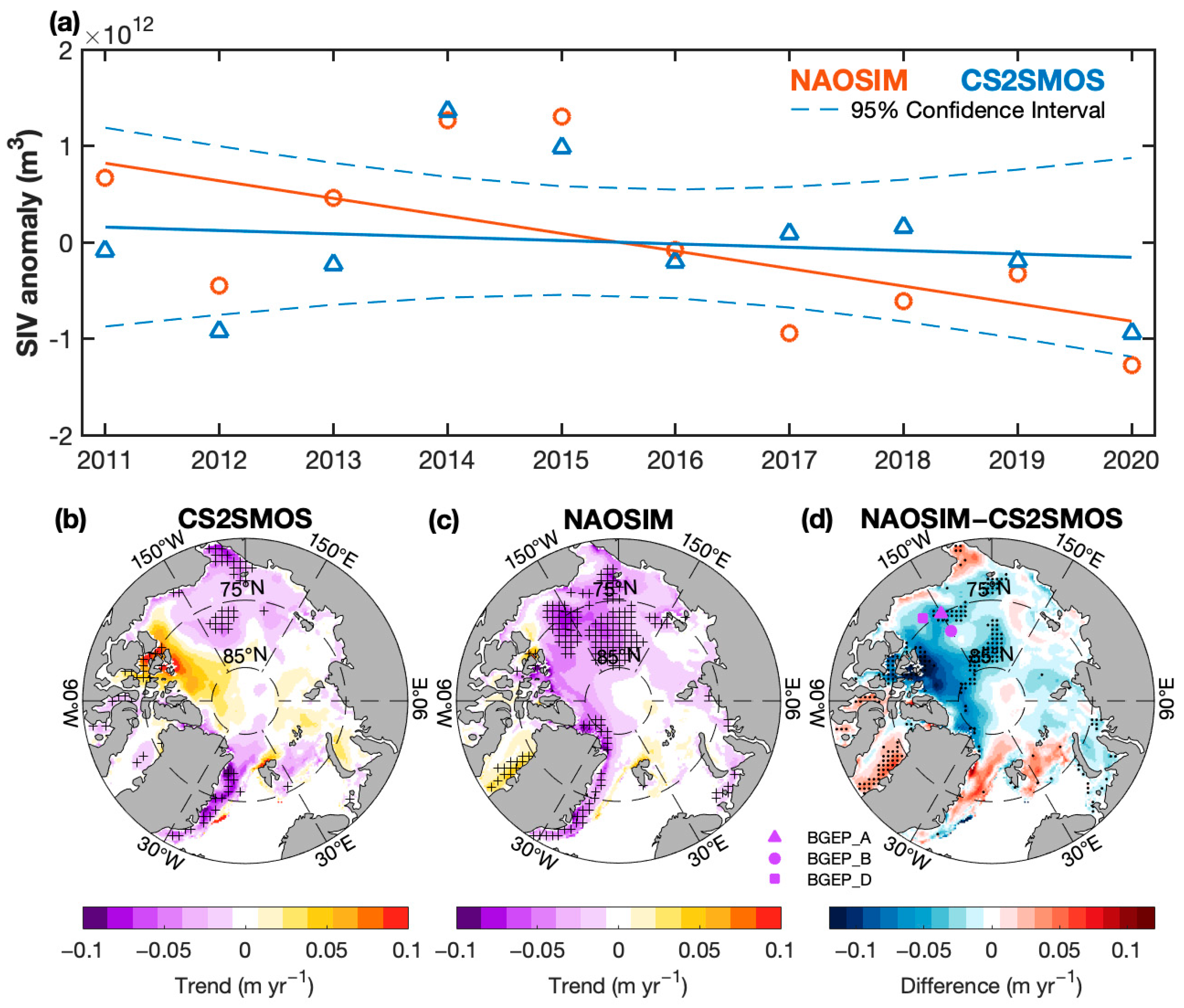
Daily averaged SIV and SIT anomalies from NAOSIM and CS2SMOS were processed into freezing period averages for obtaining a linear trend in response to the low-frequency variations in SIT. The linear trend of the freezing period average SIV anomalies and the spatial distribution of the trend in SIT anomalies of NAOSIM and CS2SMOS and their differences from 2011 to 2020 are shown in Figure 2. As Figure 2a shows, the observed SIV anomalies decrease at a slow rate (−35 km3 yr−1), a small value similar to the insignificant trend in the CryoSat-2 records from 2011 to 2018 [2]. Although the trend of NAOSIM SIV (−182 km3 yr−1) shows a more significant decline than that of the observations, it is still within the 95% confidence interval of the observations (−228 to 158 km3 yr−1). A further analysis of the spatial distribution of the SIT trends was then carried out to investigate the details of the difference in SIV trends between NAOSIM and CS2SMOS. Satellite observations of SIT anomalies show a decreasing trend in the Pacific sector and off the coast of Greenland (Figure 2b), particularly in areas near the Bering Strait and east of Greenland, where the trends passed the 95% significance test. However, there is a clear upward trend in areas around the north of the Canadian Archipelago, which has coverage of thicker ice due to regional ice convergence [52]. A generally consistent downward spatial trend in SIT anomalies from NAOSIM is shown in Figure 2c, with the fastest declines concentrated in the Beaufort Sea and along the Greenland coast, both of which passed the significance test, and only an upward trend in eastern Baffin Bay. As shown in Figure 2d, compared to the satellite results, a slower rate of decline in SIT anomalies from NAOSIM simulations is shown near the sea ice outflow passages, a faster speed is observed in the rest of the decreasing region and the upward trend in the north of the Canadian Archipelago cannot be captured by NAOSIM. Only in some regions are the differences beyond the uncertainties of the observed trends (95% confidence interval), indicating that NAOSIM can reproduce the decreasing trend in most of the Arctic. Note, however, because of the small sample sizes of the SIV and SIT anomalies, the results of the linear trend are subject to interannual variability. The SIT observations used for the optimized parameters have less interannual variability, which may lead to some spatial mismatching between NAOSIM and CS2SMOS. However, validation using higher temporal resolution data showed that although the number of samples increases from 10 to 1770, the changing trend rate is less than 2% for NAOSIM and 3% for CS2SMOS. The relative relations between NAOSIM and CS2SMOS were stable regardless of which temporal resolution of data was used, i.e., the trend of decreasing SIV was more pronounced for NAOSIM compared to CS2SMOS.
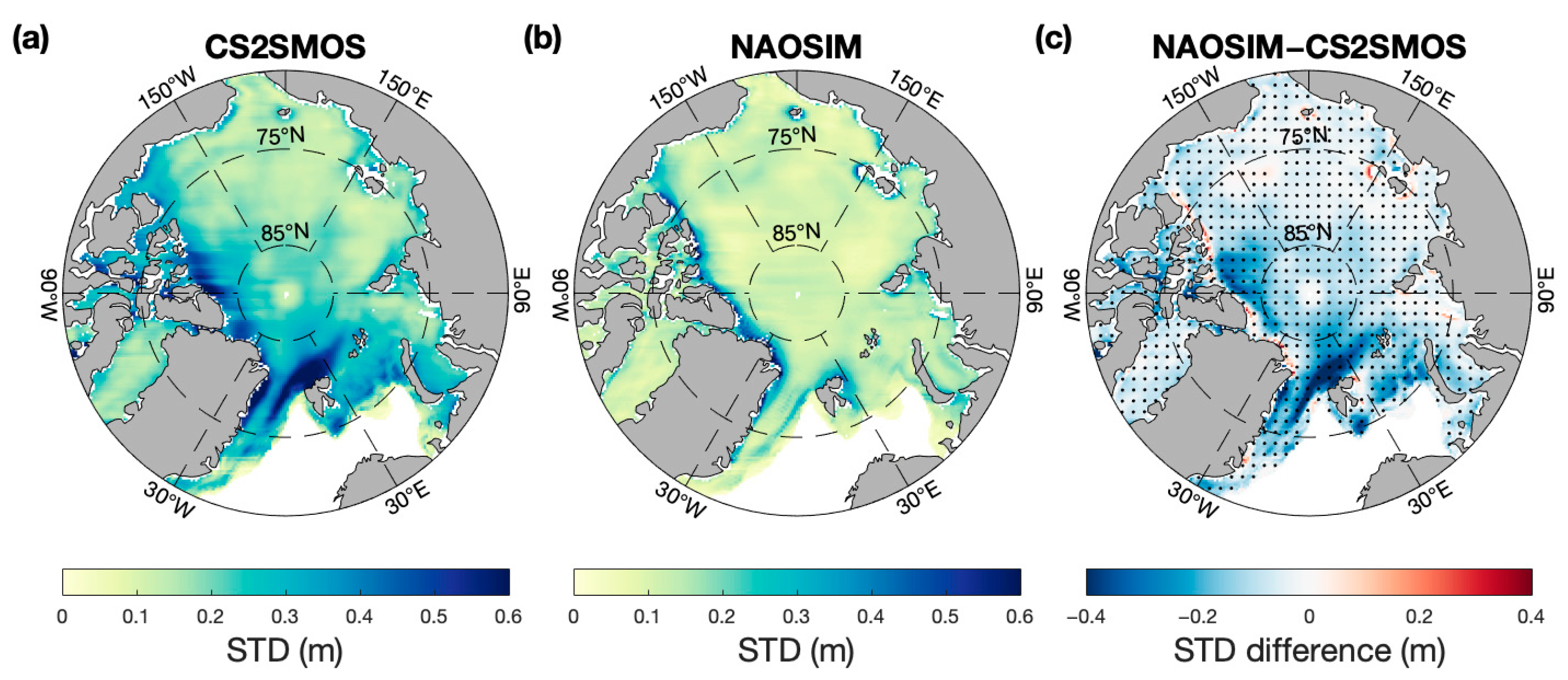
Figure 3 displays the spatial distribution and difference in the intensity of the SIT anomaly variability after detrending between NAOSIM and CS2SMOS. The trend estimates for the detrending process are based on daily averaged SIT anomaly sequences. As shown in Figure 3a, the intensity of the SIT variability in satellite observations varies widely in terms of its spatial distribution, with greater intensities in the Central Arctic and Canada–Novaya Zemlya sector compared to other areas. Especially in the north of the Canadian Archipelago and the Svalbard Islands, a large intensity SIT variability is apparent, reaching up to 0.77 m, due to the intense sea ice deformation and a large amount of sea ice outflow [53]. The intensity of the SIT variability simulated by the model is spatially consistent, with only a small area of large variability intensity off the coast of the Canadian Archipelago and Greenland, and an intensity of about 0.1 m in other areas. Compared with CS2SMOS, NAOSIM underestimates the intensity of the SIT variability in most regions, especially in the north of the Canadian Archipelago and Svalbard Islands, where sea ice changes are severe. Only a slight overestimation in the middle of the Beaufort Sea and Chukchi Sea exists. The spatial distribution of the differences in intensity of the SIT variability between NAOSIM and CS2SMOS is significant in most regions. Compared with the simulation of SIT trends, a wider spatial range of significant differences is found in the simulated intensity of SIT variability, and a uniform underestimation is shown by NAOSIM. However, the spatial distribution of intensity of SIT variability does not appear to be consistent with the SIT bias in Figure 1.
3.2. Comparison to In Situ Observations
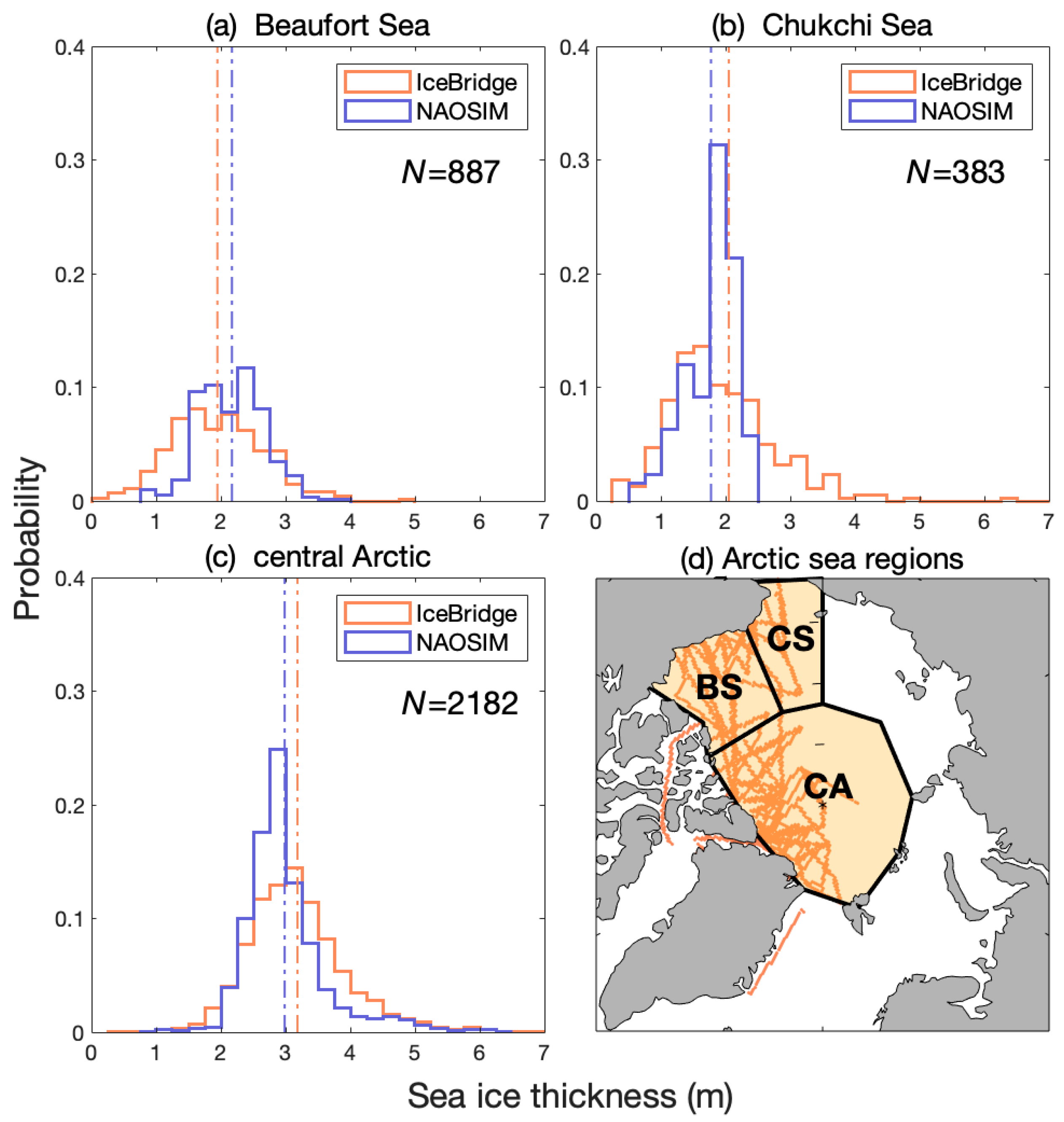
Considering the uncertainties and limited temporal coverage of satellite datasets, in situ observations were used to provide a more accurate evaluation with a broader temporal coverage. Figure 4 displays the SIT frequency distribution of NAOSIM and IceBridge observations. Compared with the mean SIT of IceBridge, it can be seen that a larger mean SIT was simulated by NAOSIM in the Beaufort Sea but a smaller mean was simulated in the Chukchi Sea and the Central Arctic, with all the biases passing the significance test (t-test with alpha = 0.05). In addition, in the Beaufort Sea, NAOSIM has a lower frequency in sea ice below 1.5 m and a higher frequency within 1.5–3 m (Figure 4a). However, a data processing bias should be noted in the IceBridge observations; IceBridge shows insufficient sensitivity to thin ice with freeboard under 0.5 m, which results in the possible underestimation of NAOSIM in the assessment [54]. SITs over 4 m and below 0.75 m cannot be clearly simulated by NAOSIM. In the Chukchi Sea, NAOSIM has a significantly higher frequency in the SIT range of 1.75–2.5 m and is unable to show ice above 2.5 m (Figure 4b). Combined with the results in Figure 1c, we can see that the model underestimates the SIT in areas close to the Bering Strait. In the central Arctic, the agreement between NAOSIM and the observed SIT is better than in the other two regions, albeit the model still has a higher frequency in the 2.5–3 m range and a lower frequency within 3–4.5 m (Figure 4c). The spatial differences in the SIT bias obtained here are close to the conclusions from CS2SMOS, confirming the results from the satellite-based analysis (Figure 1). In addition, a more concentrated SIT distribution is exhibited by NAOSIM, with larger errors in the extreme values of SIT compared to IceBridge.
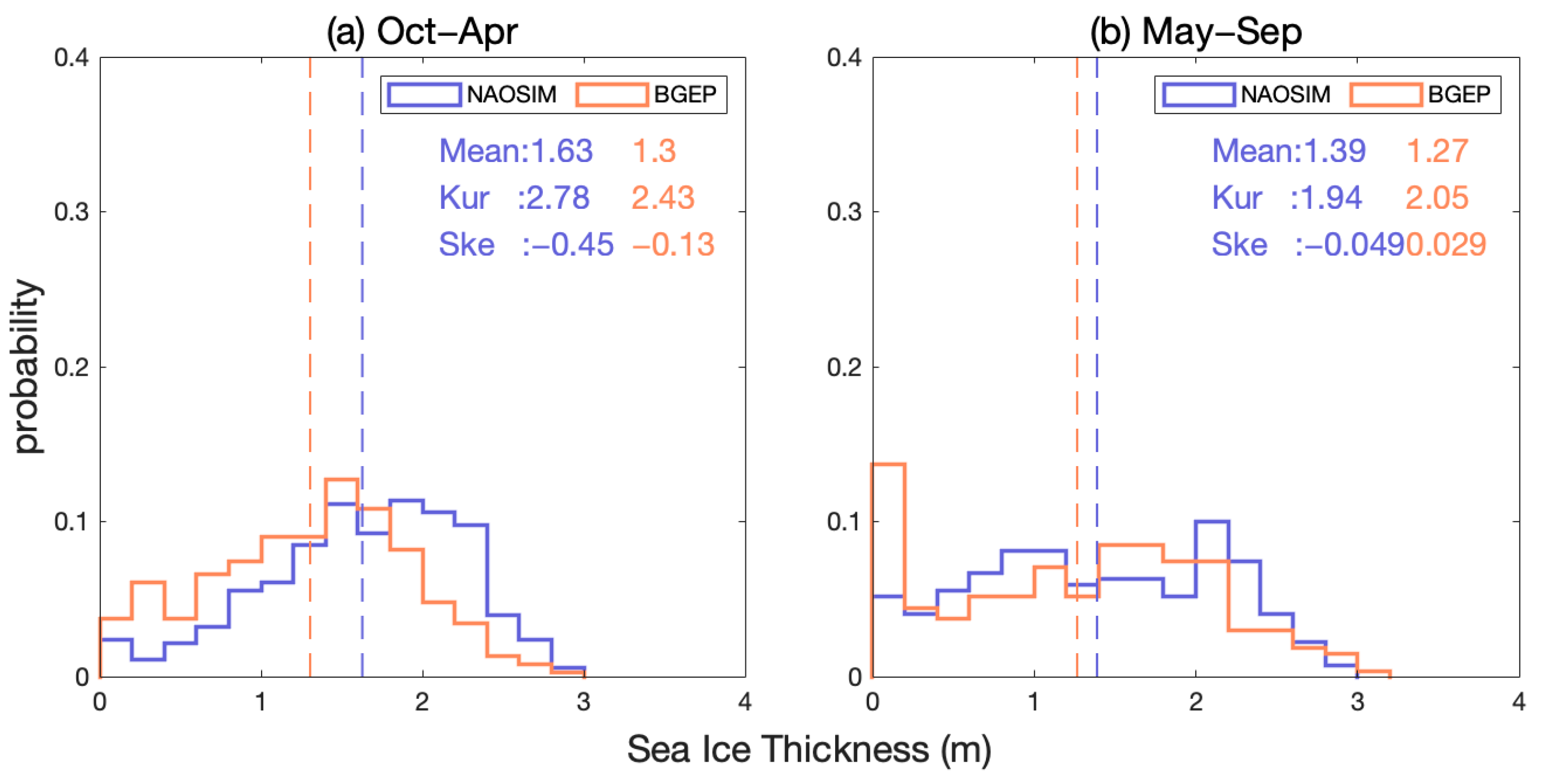
Figure 5 presents the frequency distributions of the SIT for NAOSIM and BGEP ULS in the Beaufort Sea for the freezing period (October–April) and melting period (May–September) separately. NAOSIM has a positive bias compared to the observed mean, which is consistent over both periods. The bias reaches 0.33 m during the freezing period and only 0.12 m during the melting period. In the freezing period, a left-skewed SIT distribution can be found both in NAOSIM and the observations. The asymmetric distribution of the NAOSIM SIT is more significant, showing a higher frequency of SITs greater than 1.8 m and a lower frequency of thin ice less than 1.6 m (Figure 5a). By comparing the kurtosis of NAOSIM and the observations, it can be seen that the kurtosis of NAOSIM is greater than that of the observations, which demonstrates the more concentrated distribution of the model’s SIT. In the melting period, a small positive skewness exists in the observed SIT distribution towards the minimal value zone for SIT, while an insignificant negatively skewed distribution is shown by NAOSIM (Figure 5b). The kurtosis of NAOSIM is smaller than that of the observations. It is difficult for the model to simulate the minimum SIT observed in the range of 0–0.2 m. NAOSIM consistently overestimates the SIT in the Beaufort Sea, showing more pronounced errors during the freezing period and inadequate simulations of minimum SIT values during the melting period. This analysis presents the SIT distribution difference between NAOSIM and the in situ observations in the Beaufort Sea and complements the SIT data during the melting period in this region that is lacking in CS2SMOS. Additionally, the overestimation of NAOSIM in the mean SIT in the Beaufort Sea compared with BEGP ULS confirms the conclusion from CS2SMOS.
BGEP ULS data were also used to evaluate the yearly SIT trend (Table 1). The time period chosen for the trend analysis was firstly consistent with that of CS2SMOS. During the CS2SMOS time period, a consistent downward SIT trend can be observed in both CS2SMOS and ULS at the locations of three moorings (BGEP_A, BGEP_B and BGEP_D). The decreasing rates in CS2SMOS are within the 95% confidence interval of ULS trends at BGEP_A and BGEP_B. Therefore, the SIT trends in the Beaufort Sea can be characterized by both satellite and in situ observations. NAOSIM can reproduce the decreasing trend of the SIT at all locations. A faster rate of decrease at BGEP_A is found in NAOSIM compared to the CS2SMOS- and ULS-observed trends, which slightly exceeds the 95% confidence interval of the observed trend. However, the decreasing rates in NAOSIM at BGEP_B and BGEP_D are within the 95% confidence interval of the observed trends. In terms of the rate of decline at BGEP_B and BGEP_D, however, there are more moderate decreasing rates in NAOSIM than the ULS observations, but faster than that of CS2SMOS. During the ULS period, the observed SIT also shows year-round negative trends at these three moorings. Over longer timespans, the decreasing trends of NAOSIM at all mooring locations are within the 95% confidence interval. However, the simulated rate of decline is slower than observed at all locations. In addition to validating the analysis by CS2SMOS, BGEP provides a comparison of the yearly trend and extends the temporal coverage to 2003. Analyses of both periods indicates NAOSIM can reproduce the decreasing trend of the SIT in the Beaufort Sea.
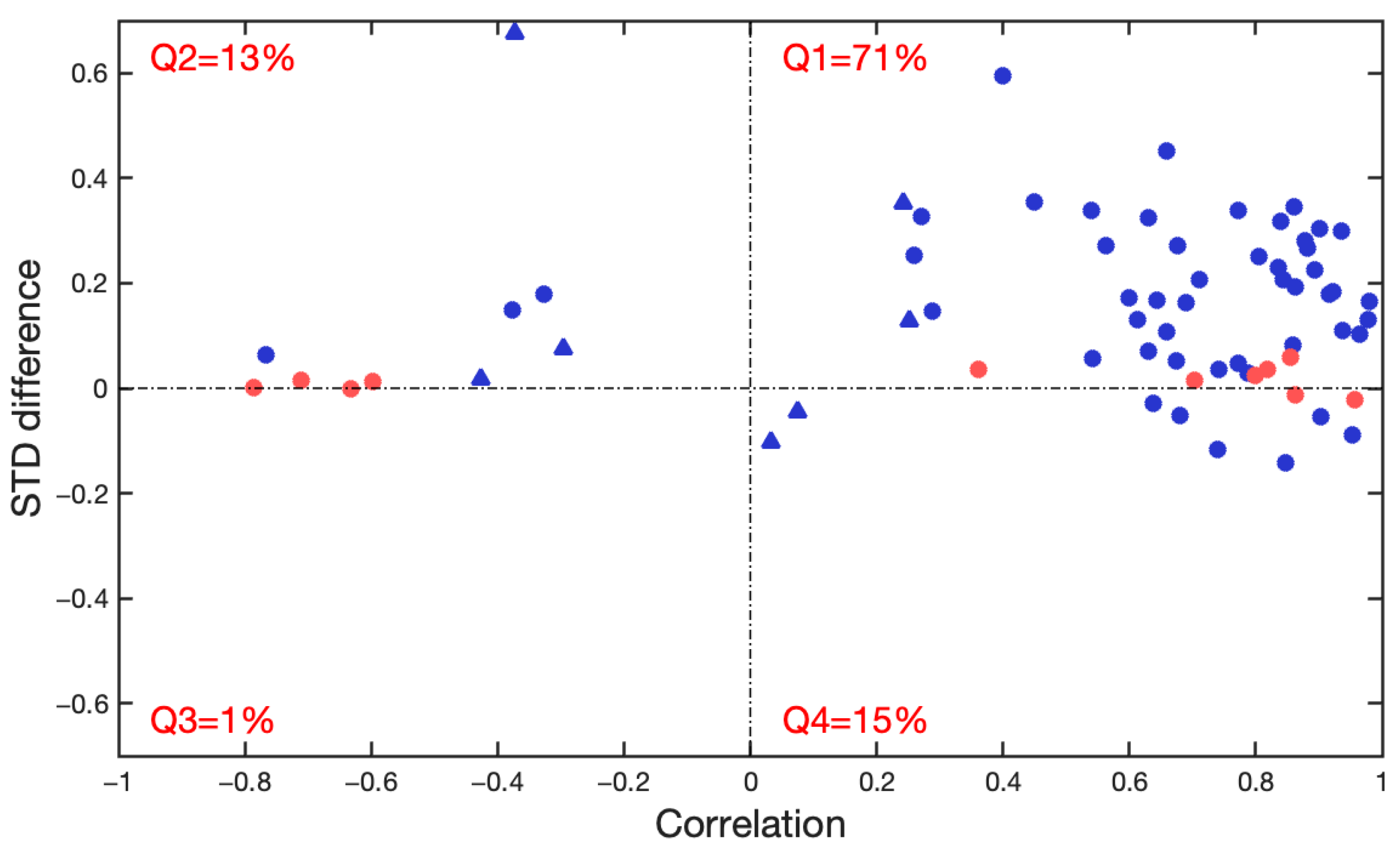
The correlation and standard deviation (STD) difference between NAOSIM and the IMB-observed SIT along 68 buoy trajectories are shown in Figure 6. By testing the correlation coefficient for 95% significance, the NAOSIM SIT for 90% of the buoys was found to be significantly correlated with the observed SIT. The NAOSIM SIT for 86% of the buoys is positively correlated with the observed SIT, and most are highly correlated. In addition, 84% of the points fall within the positive interval of the STD difference and most passed the significance test. These comparisons indicate that NAOSIM can basically simulate the thermodynamic growth in the SIT, but shows a greater intensity of variability than observed along most buoy trajectories.
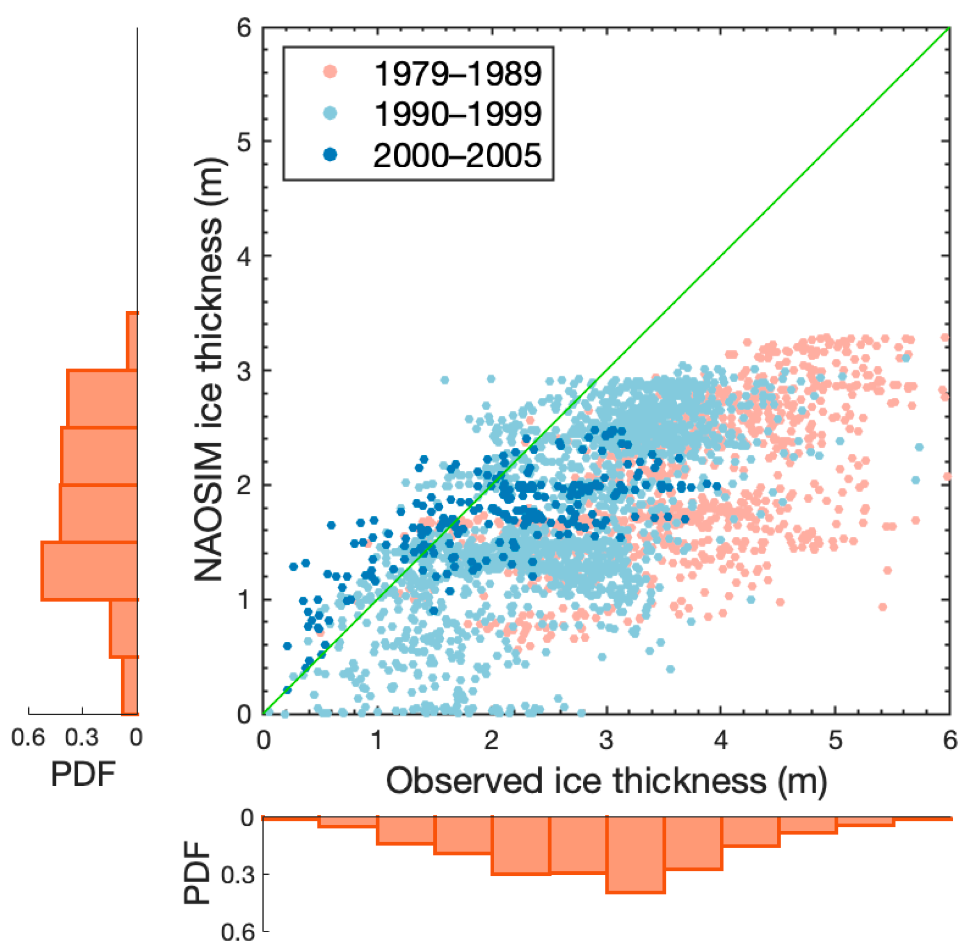
As sea ice has changed rapidly in recent years, in order to see how NAOSIM performs from 1980 to the present, submarine observations with the most overlap in time with NAOSIM were selected for analysis (Figure 7). As shown in the frequency histogram, the SIT observed by the submarines is distributed within 0–6 m and its peak is located in the interval of 3–3.5 m, basically following a Gaussian distribution. Meanwhile, the NAOSIM SIT is distributed within 0–3.5 m and the peak is located in the range of 1–1.5 m, with an obvious negative skew. The model has a low frequency in thick ice over 3 m, with a particularly insufficient simulation ability for sea ice thicker than 3.5 m. NAOSIM significantly underestimates the SIT during 1979–2005. Considering the rapid change in SIT, the results were divided into three groups by decade (shown in Figure 7) to explore whether the underestimation of the model differs in different decades. It can be seen from the scatterplot that a thinner sea ice is simulated by NAOSIM overall, and this is more pronounced before 2000. In the years closer to 2000, the scatter moves close to the 1:1 line and the underestimation of the model gradually decreases. After 2000, although the amplitude of underestimation decreases, NAOSIM still overestimates the SIT for thin ice (>1.5 m) and underestimates it for thick ice (<1.5 m). It can be seen that the model performs better with time closer to the optimization window of the SIT (2000–2012), indicating parameter optimization that is dependent on the choice of optimization window.
4. Conclusions
A long-term daily NAOSIM SIT was produced from simulations with simultaneous parameter optimization. In this study, the NAOSIM SIT data were evaluated against satellite and in situ observations. Although multiple types of observations are used as reference datasets in this study, these observations both complement and validate each other in terms of spatial and temporal distribution and the physical processes of concern. The present results show that the multi-source observations are self-consistent with each other, which makes it possible to evaluate the NAOSIM SIT from several perspectives based on the above data, and the conclusions are consistent. In general, NAOSIM can basically reproduce the annual cycle and downward trend in SIV. In detail, NAOSIM can reproduce the annual growth in the Arctic SIV during the freezing period and can qualitatively estimate the downward trend in the SIV and SIT measured by the observations in most regions of the Arctic. Although the trend differs from the observed values, it is within the 95% confidence interval. Additionally, in terms of SIT thermodynamics, the thermodynamic growth in the SIT in NAOSIM is highly correlated with that of the IMB observations. These results suggest that NAOSIM can be used to study the variation in Arctic sea ice over time.
However, deficiencies can still be found in NAOSIMs simulation of SIT spatial patterns compared with satellite and in situ observations. This is mainly reflected in the SIT overestimation of thin ice (<1.5 m) in the Beaufort Sea and the underestimation of thick ice (>1.5 m) in the central Arctic during the freezing period. In addition, the sea ice distribution of NAOSIM is more concentrated and errors appear especially at extreme SITs. Compared to the BGEP ULS observations, although NAOSIM always presents a thicker ice in the Beaufort Sea, the error during the melting period is smaller than that in the freezing period. Furthermore, a mismatch in the trend and intensity of variability can still be found between NAOSIM and the observations. NAOSIM is unable to capture the upward trend in the SIT in the north of the Canadian Archipelago and the spatial difference in the intensity of the SIT variability. Additionally, it underestimates the intensity of the SIT variability in most regions, especially in the areas with severe sea ice changes. Using smoothed SIT observations without interannual variability for optimization may affect these simulations. Notably, compared to submarine observations over a longer time span, although NAOSIM produces an overall underestimation of the SIT before 2000, it performs better at times closer to the optimization window (2000–2012), suggesting parameter optimization that is dependent on the choice of optimization window. In the context of global warming, the nature of Arctic sea ice properties is changing rapidly [55]. The limited temporal coverage of SIT observations chosen for parameter optimization makes it difficult for the model to accurately simulate the different sea ice variability over different decades. Therefore, it is important to know how to better optimize the parameters used in model simulations of sea ice based on limited observations under this rapid change, which may help to improve the accuracy of estimated Arctic SIT and provide support to further research related to Arctic sea ice.
In addition, the limited temporal sampling of Arctic SIT observations used in this study for evaluation cannot be ignored. Although the temporal resolution of CS2SMOS is better compared to the other satellite datasets, the seven day averaged product cannot be completely consistent with the daily SIT from NAOSIM. The observations are unevenly distributed over time, with all datasets concentrated after 2000 except for the data from submarines. All these limitations will affect the accuracy of the assessment. Therefore, with the development of observational datasets, more accurate estimations of Arctic SIT can be expected to improve the reliability of such evaluations.
Author Contributions
Q.Y. and H.L. conceptualized this study; Q.Z., H.L. and C.M. carried out the study, performed the calculations and drafted the paper; Y.X. and Q.S. helped with data processing; H.L., C.M. and Q.Y. reviewed and edited the paper. All authors have read and agreed to the published version of the manuscript.
Funding
This study was funded by Southern Marine Science and Engineering Guangdong Laboratory (Zhuhai) (No. SML2021SP312), the National Key R&D Program of China (no. 2022YFE0106300), the Guangdong Basic and Applied Basic Research Foundation (no. 2020B1515020025), the Program of Marine Economy Development Special Fund under Department of Natural Resources of Guangdong Province (no. GDNRC [2022]18) and the fundamental research funds for the Norges Forskningsråd (no. 328886).
Data Availability Statement
The CS2SMOS sea ice thickness data can be downloaded from https://data.seaiceportal.de/data/cs2smos_awi/ (accessed on 13 December 2021). The in situ observational datasets including IceBridge, BGEP ULS and submarines can be downloaded from http://psc.apl.washington.edu/sea_ice_cdr/data_tables.html (accessed on 3 November 2021). The IMB dataset can be downloaded from http://imb-crrel-dartmouth.org/archived-data/ (accessed on 3 November 2021).
Acknowledgments
This is a contribution to the Year of Polar Prediction (YOPP), a flagship activity of the Polar Prediction Project (PPP), initiated by the World Weather Research Program (WWRP) of the World Meteorological Organization (WMO). We acknowledge the WMO WWRP for its role in coordinating this International Research activity. We also gratefully thank Frank Kauker from the Alfred Wegener Institute for providing the NAOSIM model data. The merging of the CryoSat–SMOS sea ice thickness data was funded by the ESA project SMOS& CryoSat-2 Sea Ice Data Product Processing and Dissemination Service, and data from DATE to DATE were obtained from AWI.
Conflicts of Interest
The authors declare no conflict of interest.
References
- Serreze, M.C.; Meier, W.N. The Arctic’s sea ice cover: Trends, variability, predictability, and comparisons to the Antarctic. Ann. N. Y. Acad. Sci. 2019, 1436, 36–53. [Google Scholar] [CrossRef] [PubMed]
- Kwok, R. Arctic sea ice thickness, volume, and multiyear ice coverage: Losses and coupled variability (1958–2018). Environ. Res. Lett. 2018, 13, 105005. [Google Scholar] [CrossRef]
- Meier, W.N.; Hovelsrud, G.K.; van Oort, B.E.H.; Key, J.R.; Kovacs, K.M.; Michel, C.; Haas, C.; Granskog, M.A.; Gerland, S.; Perovich, D.K.; et al. Arctic sea ice in transformation: A review of recent observed changes and impacts on biology and human activity. Rev. Geophys. 2014, 52, 185–217. [Google Scholar] [CrossRef]
- Melia, N.; Haines, K.; Hawkins, E.; Day, J.J. Towards seasonal Arctic shipping route predictions. Environ. Res. Lett. 2017, 12, 084005. [Google Scholar] [CrossRef]
- Min, C.; Yang, Q.; Chen, D.; Yang, Y.; Zhou, X.; Shu, Q.; Liu, J. The Emerging Arctic Shipping Corridors. Geophys. Res. Lett. 2022, 49, e2022GL099157. [Google Scholar] [CrossRef]
- Min, C.; Zhou, X.; Luo, H.; Yang, Y.; Wang, Y.; Zhang, J.; Yang, Q. Toward Quantifying the Increasing Accessibility of the Arctic Northeast Passage in the Past Four Decades. Adv. Atmos. Sci. 2023. [Google Scholar] [CrossRef]
- Kurtz, N.T.; Markus, T.; Farrell, S.L.; Worthen, D.L.; Boisvert, L.N. Observations of recent Arctic sea ice volume loss and its impact on ocean-atmosphere energy exchange and ice production. J. Geophys. Res. Ocean. 2011, 116, C04015. [Google Scholar] [CrossRef]
- Rothrock, D.A.; Yu, Y.; Maykut, G.A. Thinning of the Arctic sea-ice cover. Geophys. Res. Lett. 1999, 26, 3469–3472. [Google Scholar] [CrossRef]
- Rothrock, D.A.; Percival, D.B.; Wensnahan, M. The decline in arctic sea-ice thickness: Separating the spatial, annual, and interannual variability in a quarter century of submarine data. J. Geophys. Res. 2008, 113, C05003. [Google Scholar] [CrossRef]
- Melling, H.; Riedel, D.A.; Gedalof, Z.E. Trends in the draft and extent of seasonal pack ice, Canadian Beaufort Sea. Geophys. Res. Lett. 2005, 32, L24501. [Google Scholar] [CrossRef]
- Kurtz, N.T.; Farrell, S.L.; Studinger, M.; Galin, N.; Harbeck, J.P.; Lindsay, R.; Onana, V.D.; Panzer, B.; Sonntag, J.G. Sea ice thickness, freeboard, and snow depth products from Operation IceBridge airborne data. Cryosphere 2013, 7, 1035–1056. [Google Scholar] [CrossRef]
- Haas, C.; Lobach, J.; Hendricks, S.; Rabenstein, L.; Pfaffling, A. Helicopter-borne measurements of sea ice thickness, using a small and lightweight, digital EM system. J. Appl. Geophys. 2009, 67, 234–241. [Google Scholar] [CrossRef]
- Polashenski, C.; Perovich, D.; Richter-Menge, J.; Elder, B. Seasonal ice mass-balance buoys: Adapting tools to the changing Arctic. Ann. Glaciol. 2011, 52, 18–26. [Google Scholar] [CrossRef]
- Kwok, R.; Cunningham, G.F. ICESat over Arctic sea ice: Estimation of snow depth and ice thickness. J. Geophys. Res. Ocean. 2008, 113, C08010. [Google Scholar] [CrossRef]
- Laxon, S.W.; Giles, K.A.; Ridout, A.L.; Wingham, D.J.; Willatt, R.; Cullen, R.; Kwok, R.; Schweiger, A.; Zhang, J.; Haas, C.; et al. CryoSat-2 estimates of Arctic sea ice thickness and volume. Geophys. Res. Lett. 2013, 40, 732–737. [Google Scholar] [CrossRef]
- Markus, T.; Neumann, T.; Martino, A.; Abdalati, W.; Brunt, K.; Csatho, B.; Farrell, S.; Fricker, H.; Gardner, A.; Harding, D.; et al. The Ice, Cloud, and land Elevation Satellite-2 (ICESat-2): Science requirements, concept, and implementation. Remote Sens. Environ. 2017, 190, 260–273. [Google Scholar] [CrossRef]
- Zhang, S.; Xuan, Y.; Li, J.; Geng, T.; Li, X.; Xiao, F. Arctic Sea Ice Freeboard Retrieval from Envisat Altimetry Data. Remote Sens. 2021, 13, 1414. [Google Scholar] [CrossRef]
- Laxon, S.; Peacock, N.; Smith, D. High interannual variability of sea ice thickness in the Arctic region. Nature 2003, 425, 947–950. [Google Scholar] [CrossRef] [PubMed]
- Tian-Kunze, X.; Kaleschke, L.; Maaß, N.; Mäkynen, M.; Serra, N.; Drusch, M.; Krumpen, T. SMOS-derived thin sea ice thickness: Algorithm baseline, product specifications and initial verification. Cryosphere 2014, 8, 997–1018. [Google Scholar] [CrossRef]
- Landy, J.C.; Dawson, G.J.; Tsamados, M.; Bushuk, M.; Stroeve, J.C.; Howell, S.E.L.; Krumpen, T.; Babb, D.G.; Komarov, A.S.; Heorton, H.; et al. A year-round satellite sea-ice thickness record from CryoSat-2. Nature 2022, 609, 517–522. [Google Scholar] [CrossRef]
- Zheng, F.; Sun, Y.; Yang, Q.; Mu, L. Evaluation of Arctic Sea-ice Cover and Thickness Simulated by MITgcm. Adv. Atmos. Sci. 2021, 38, 29–48. [Google Scholar] [CrossRef]
- Chen, L.; Wu, R.; Shu, Q.; Min, C.; Yang, Q.; Han, B. The Arctic Sea Ice Thickness Change in CMIP6′s Historical Simulations. Adv. Atmos. Sci. 2023, 1–3. [Google Scholar] [CrossRef]
- Schweiger, A.; Lindsay, R.; Zhang, J.; Steele, M.; Stern, H.; Kwok, R. Uncertainty in modeled Arctic sea ice volume. J. Geophys. Res. 2011, 116, C00D06. [Google Scholar] [CrossRef]
- Sumata, H.; Kauker, F.; Karcher, M.; Gerdes, R. Covariance of Optimal Parameters of an Arctic Sea Ice–Ocean Model. Mon. Weather. Rev. 2019, 147, 2579–2602. [Google Scholar] [CrossRef]
- Kim, J.G.; Hunke, E.C.; Lipscomb, W.H. Sensitivity analysis and parameter tuning scheme for global sea-ice modeling. Ocean. Model. 2006, 14, 61–80. [Google Scholar] [CrossRef]
- Nguyen, A.T.; Menemenlis, D.; Kwok, R. Arctic ice-ocean simulation with optimized model parameters: Approach and assessment. J. Geophys. Res. Ocean. 2011, 116, C04025. [Google Scholar] [CrossRef]
- Sumata, H.; Kauker, F.; Gerdes, R.; Köberle, C.; Karcher, M. A comparison between gradient descent and stochastic approaches for parameter optimization of a sea ice model. Ocean. Sci. 2013, 9, 609–630. [Google Scholar] [CrossRef]
- Sumata, H.; Kauker, F.; Karcher, M.; Gerdes, R. Simultaneous Parameter Optimization of an Arctic Sea Ice–Ocean Model by a Genetic Algorithm. Mon. Weather. Rev. 2019, 147, 1899–1926. [Google Scholar] [CrossRef]
- Ricker, R.; Kauker, F.; Schweiger, A.; Hendricks, S.; Zhang, J.; Paul, S. Evidence for an increasing role of ocean heat in Arctic winter sea ice growth. J. Clim. 2021, 34, 5215–5227. [Google Scholar] [CrossRef]
- Wingham, D.J.; Francis, C.R.; Baker, S.; Bouzinac, C.; Brockley, D.; Cullen, R.; de Chateau-Thierry, P.; Laxon, S.W.; Mallow, U.; Mavrocordatos, C.; et al. CryoSat: A mission to determine the fluctuations in Earth’s land and marine ice fields. Adv. Space Res. 2006, 37, 841–871. [Google Scholar] [CrossRef]
- Lindsay, R.; Schweiger, A. Arctic sea ice thickness loss determined using subsurface, aircraft, and satellite observations. Cryosphere 2015, 9, 269–283. [Google Scholar] [CrossRef]
- Min, C.; Yang, Q.; Mu, L.; Kauker, F.; Ricker, R. Ensemble-based estimation of sea-ice volume variations in the Baffin Bay. Cryosphere 2021, 15, 169–181. [Google Scholar] [CrossRef]
- Yang, Y.; Min, C.; Luo, H.; Kauker, F.; Ricker, R.; Yang, Q. The evolution of the Fram Strait sea ice volume export decomposed by age: Estimating with parameter-optimized sea ice-ocean model outputs. Environ. Res. Lett. 2022, 18, 014029. [Google Scholar] [CrossRef]
- Hibler, W.D. A Dynamic Thermodynamic Sea Ice Model. J. Phys. Oceanogr. 1979, 9, 815–846. [Google Scholar] [CrossRef]
- Pacanowski, R.C. Documentation user’s guide and reference manual (MOM2, Version 2). GFDL Ocean. Tech. Rep. 1996, 329. [Google Scholar]
- Hibler, W.D.; Bryan, K. A Diagnostic Ice–Ocean Model. J. Phys. Oceanogr. 1987, 17, 987–1015. [Google Scholar] [CrossRef]
- Saha, S.; Moorthi, S.; Wu, X.; Wang, J.; Nadiga, S.; Tripp, P.; Behringer, D.; Hou, Y.-T.; Chuang, H.-Y.; Iredell, M.; et al. The NCEP Climate Forecast System Version 2. J. Clim. 2014, 27, 2185–2208. [Google Scholar] [CrossRef]
- Eastwood, S.; Jenssen, M.; Lavergne, T.; Sørensen, A.M.; Tonboe, R. Global Sea Ice Concentration Reprocessing: Product User Manual. Product OSI-409, OSI-409-a, OSI-430. Available online: http://osisaf.met.no/docs/osisaf_cdop3_ss2_pum_sea-ice-conc-reproc_v2p5.pdf (accessed on 15 February 2023).
- Lavergne, T.; Eastwood, S.; Teffah, Z.; Schyberg, H.; Breivik, L.-A. Sea ice motion from low-resolution satellite sensors: An alternative method and its validation in the Arctic. J. Geophys. Res. Ocean. 2010, 115, C10032. [Google Scholar] [CrossRef]
- Kimura, N.; Nishimura, A.; Tanaka, Y.; Yamaguchi, H. Influence of winter sea-ice motion on summer ice cover in the Arctic. Polar Res. 2013, 32, 20193. [Google Scholar] [CrossRef]
- Fowler, C.; Maslanik, J.; Emery, W.; Tschudi, M. Polar Pathfinder Daily 25 km EASE-Grid Sea Ice Motion Vectors, Version 2; National Snow and Ice Data Center: Boulder, CL, USA, 2013. [Google Scholar] [CrossRef]
- Tschudi, M.; Fowler, C.; Maslanik, J.; Stroeve, J. Tracking the Movement and Changing Surface Characteristics of Arctic Sea Ice. IEEE J. Sel. Top. Appl. Earth Obs. Remote Sens. 2010, 3, 536–540. [Google Scholar] [CrossRef]
- Ricker, R.; Hendricks, S.; Kaleschke, L.; Tian-Kunze, X.; King, J.; Haas, C. A weekly Arctic sea-ice thickness data record from merged CryoSat-2 and SMOS satellite data. Cryosphere 2017, 11, 1607–1623. [Google Scholar] [CrossRef]
- Ricker, R. CryoSat-2/SMOS Merged Product Description Document (PDD). Available online: https://spaces.awi.de/download/attachments/297634429/AWI_ESA_CS2SMOS_PDD_v1.2.pdf (accessed on 15 February 2023).
- Hendricks, S. CryoSat-2/SMOS Merged Product Description Document (PDD). Available online: https://earth.esa.int/eogateway/documents/20142/37627/CryoSat-2-SMOS-Merged-Product-Description-Document-PDD.pdf (accessed on 15 February 2023).
- Kurtz, N.; Studinger, M.; Harbeck, J.; Onana, V.; Yi, D. IceBridge L4 Sea Ice Freeboard, Snow Depth, and Thickness, Version 1; NASA DAAC at the National Snow and Ice Data Center: Boulder, CL, USA, 2015. [CrossRef]
- Richter-Menge, J.A.; Perovich, D.K.; Elder, B.C.; Claffey, K.; Rigor, I.; Ortmeyer, M. Ice mass-balance buoys: A tool for measuring and attributing changes in the thickness of the Arctic sea-ice cover. Ann. Glaciol. 2006, 44, 205–210. [Google Scholar] [CrossRef]
- Perovich, D.; Richter-Menge, J.A. From points to Poles: Extrapolating point measurements of sea-ice mass balance. Ann. Glaciol. 2017, 44, 188–192. [Google Scholar] [CrossRef]
- Melling, H.; Johnston, P.H.; Riedel, D.A. Measurements of the Underside Topography of Sea Ice by Moored Subsea Sonar. J. Atmos. Ocean. Technol. 1995, 12, 589–602. [Google Scholar] [CrossRef]
- Wensnahan, M.; Rothrock, D.A. Sea-ice draft from submarine-based sonar: Establishing a consistent record from analog and digitally recorded data. Geophys. Res. Lett. 2005, 32, L11502. [Google Scholar] [CrossRef]
- Wensnahan, M.; Rothrock, D.A. The Accuracy of Sea Ice Drafts Measured from U.S. Navy Submarines. J. Atmos. Ocean. Technol. 2007, 24, 1936–1949. [Google Scholar] [CrossRef]
- Kwok, R. Sea ice convergence along the Arctic coasts of Greenland and the Canadian Arctic Archipelago: Variability and extremes (1992–2014). Geophys. Res. Lett. 2015, 42, 7598–7605. [Google Scholar] [CrossRef]
- Kwok, R. Outflow of Arctic Ocean Sea Ice into the Greenland and Barents Seas: 1979–2007. J. Clim. 2009, 22, 2438–2457. [Google Scholar] [CrossRef]
- Zhang, S.; Geng, T.; Zhu, C.; Li, J.; Li, X.; Zhu, B.; Liu, L.; Xiao, F. Arctic Sea Ice Freeboard Estimation and Variations from Operation IceBridge. IEEE Trans. Geosci. Remote Sens. 2022, 60, 1–10. [Google Scholar] [CrossRef]
- Ogawa, F.; Keenlyside, N.; Gao, Y.; Koenigk, T.; Yang, S.; Suo, L.; Wang, T.; Gastineau, G.; Nakamura, T.; Cheung, H.N.; et al. Evaluating Impacts of Recent Arctic Sea Ice Loss on the Northern Hemisphere Winter Climate Change. Geophys. Res. Lett. 2018, 45, 3255–3263. [Google Scholar] [CrossRef]
Figure 1.
The annual cycle of sea ice volume (SIV) and the annual mean sea ice thickness (SIT) bias of the North Atlantic/Arctic Ocean–Sea Ice Model (NAOSIM) against CS2SMOS (merged CryoSat-2 and SMOS (Soil Moisture Ocean Salinity satellite) SIT product)] in the freezing period. In (a), the orange and blue lines denote the SIV related to NAOSIM and CS2SMOS, respectively. The shaded areas denote the uncertainty of the satellite SIV. (b) SIT Bias (2011–2020) from October to December between NAOSIM and CS2SMOS. The black contours indicate the average SIT of NAOSIM, while the dotted areas denote where the bias is beyond the uncertainties of CS2SMOS. (c) As in (b) but from January to April.

Figure 2.
The (a) linear trend of freezing period average SIV anomalies, spatial distribution of the trend in SIT anomalies of (b) CS2SMOS and (c) NAOSIM and (d) difference in the trend between NAOSIM and CS2SMOS from 2011 to 2020. The orange and blue solid lines denote the SIV trend lines related to NAOSIM and CS2SMOS, respectively, and the blue dotted lines denote the 95% confidence interval of CS2SMOS. The plus signs in (b,c) indicate areas where the trends pass the 95% significance test. The dotted areas in (d) are where the difference is beyond the 95% confidence intervals for the satellite trends.

Figure 3.
Spatial distribution of the standard deviation (STD) of daily SIT anomalies of (a) CS2SMOS and (b) NAOSIM, and (c) the STD difference between them. The dotted areas in (c) are where the STD difference passes the significance test (F-test with alpha = 0.1).
Figure 3.
Spatial distribution of the standard deviation (STD) of daily SIT anomalies of (a) CS2SMOS and (b) NAOSIM, and (c) the STD difference between them. The dotted areas in (c) are where the STD difference passes the significance test (F-test with alpha = 0.1).

Figure 4.
Probability histogram of the NAOSIM SIT and the IceBridge SIT in (a) the Beaufort Sea (BS), (b) the Chukchi Sea (CS) and (c) the central Arctic (CA), along with (d) a schematic map of the observational trajectories and three individual Arctic sea regions. The blue (red) stair-shaped plots represent the NAOSIM (IceBridge) ice thickness. The dashed lines indicate the mean SIT of the datasets. The bin size is 0.25 m and the probability distribution is normalized. N refers to the number of grids in which observations are located.

Figure 5.
Probability histograms of the SIT for NAOSIM and Beaufort Gyre Exploration Project (BGEP) upward-looking sonar (ULS) observations in (a) October–April (freezing period) and (b) May–September (melting period). The blue (red) stair-shaped plots represent the SIT of NAOSIM (BGEP ULS). The dashed lines indicate the mean SIT of the datasets. The bin size is 0.2 m and the probability distribution is normalized. N refers to the number of samples, and Mean, Kur and Ske refer to the mean value, kurtosis and skewness of the SIT probability distribution, respectively.

Figure 6.
The correlation and STD difference between NAOSIM SIT and IMB (ice mass balance) observations along 68 buoy trajectories. Circles (triangles) indicate that the correlation coefficient passed (failed) the 95% significance test. Blue (red) points indicate that the STD difference passed (failed) the significance test (F-test with alpha = 0.1). The red text indicates the percentage of circles located in different quadrants.

Figure 7.
Probability density histogram (PDF) and scatterplot comparing NAOSIM and submarine observations. The years are divided into three decades (1979–1989, 1990–1999 and 2000–2005).
Figure 7.
Probability density histogram (PDF) and scatterplot comparing NAOSIM and submarine observations. The years are divided into three decades (1979–1989, 1990–1999 and 2000–2005).


Table 1.
Linear trends (m yr−1) of NAOSIM, CS2SMOS and observed SIT anomalies at different mooring locations and periods with corresponding 95% confidence intervals for observed trends. The CS2SMOS period is October–April 2011 to 2020 and the ULS period is 2003–2020.
Table 1.
Linear trends (m yr−1) of NAOSIM, CS2SMOS and observed SIT anomalies at different mooring locations and periods with corresponding 95% confidence intervals for observed trends. The CS2SMOS period is October–April 2011 to 2020 and the ULS period is 2003–2020.
| Mooring | Trend in CS2SMOS Period | Trend in ULS Period |
|---|---|---|
| BGEP_A | −0.043 ± 0.030 | −0.045 ± 0.018 |
| CS2SMOS_A | −0.016 | |
| NAOSIM_A | −0.075 | −0.044 |
| BGEP_B | −0.051 ± 0.034 | −0.062 ± 0.018 |
| CS2SMOS_B | −0.029 | |
| NAOSIM_B | −0.046 | −0.047 |
| BGEP_D | −0.076 ± 0.044 | −0.059 ± 0.028 |
| CS2SMOS_D | −0.017 | |
| NAOSIM_D | −0.050 | −0.040 |
Disclaimer/Publisher’s Note: The statements, opinions and data contained in all publications are solely those of the individual author(s) and contributor(s) and not of MDPI and/or the editor(s). MDPI and/or the editor(s) disclaim responsibility for any injury to people or property resulting from any ideas, methods, instructions or products referred to in the content. |
© 2023 by the authors. Licensee MDPI, Basel, Switzerland. This article is an open access article distributed under the terms and conditions of the Creative Commons Attribution (CC BY) license (https://creativecommons.org/licenses/by/4.0/).
Share and Cite
MDPI and ACS Style
Zhang, Q.; Luo, H.; Min, C.; Xiu, Y.; Shi, Q.; Yang, Q. Evaluation of Arctic Sea Ice Thickness from a Parameter-Optimized Arctic Sea Ice–Ocean Model. Remote Sens. 2023, 15, 2537. https://doi.org/10.3390/rs15102537
AMA Style
Zhang Q, Luo H, Min C, Xiu Y, Shi Q, Yang Q. Evaluation of Arctic Sea Ice Thickness from a Parameter-Optimized Arctic Sea Ice–Ocean Model. Remote Sensing. 2023; 15(10):2537. https://doi.org/10.3390/rs15102537
Chicago/Turabian StyleZhang, Qiaoqiao, Hao Luo, Chao Min, Yongwu Xiu, Qian Shi, and Qinghua Yang. 2023. "Evaluation of Arctic Sea Ice Thickness from a Parameter-Optimized Arctic Sea Ice–Ocean Model" Remote Sensing 15, no. 10: 2537. https://doi.org/10.3390/rs15102537
Note that from the first issue of 2016, this journal uses article numbers instead of page numbers. See further details here.