

Comparing Thermal Regime Stages along a Small Yakutian Fluvial Valley with Point Scale Measurements, Thermal Modeling, and Near Surface Geophysics
 , , , , , , , , , , ,
Abstract
:1. Introduction
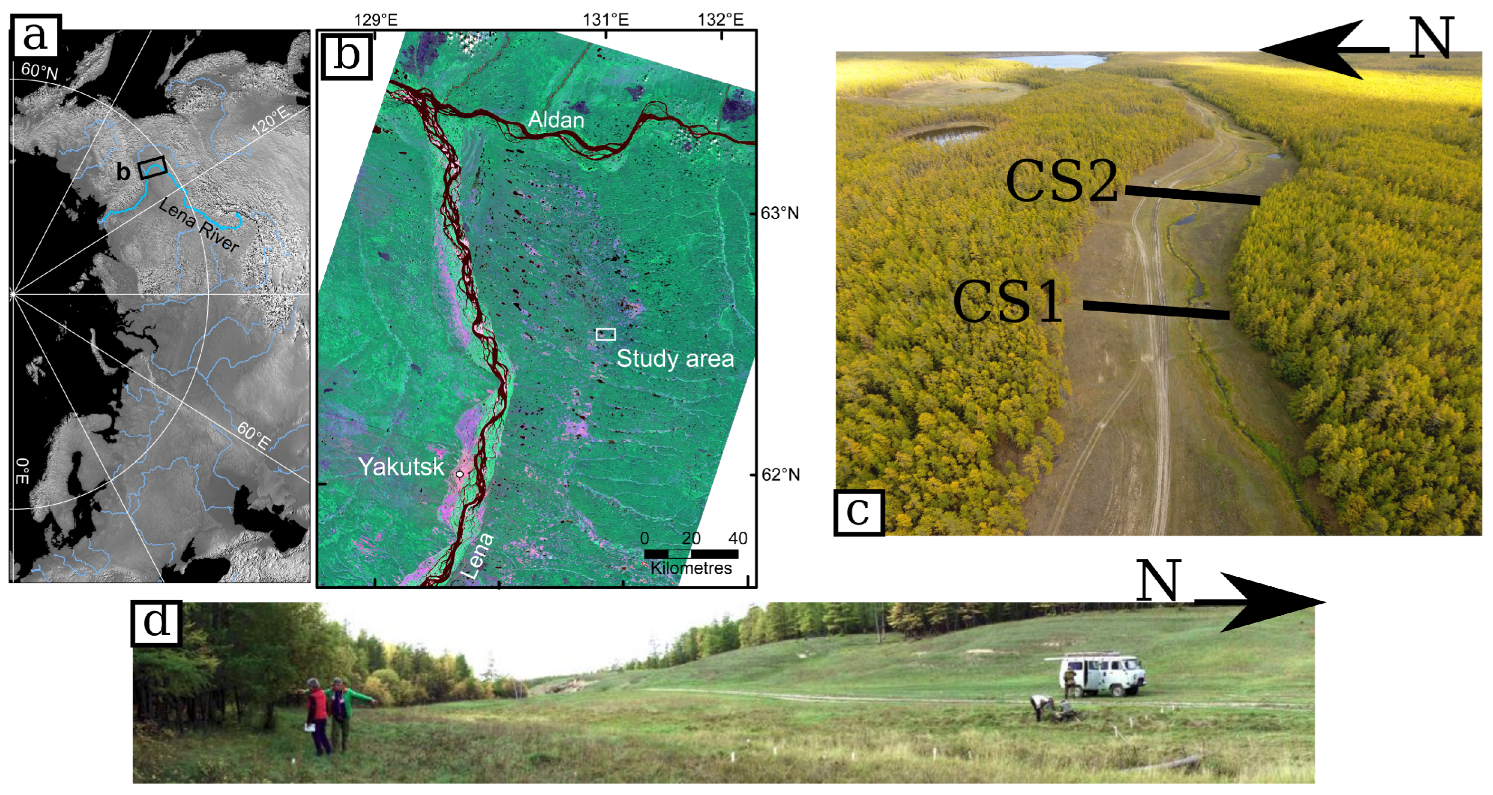
2. Area and Site Descriptions
3. Materials and Methods
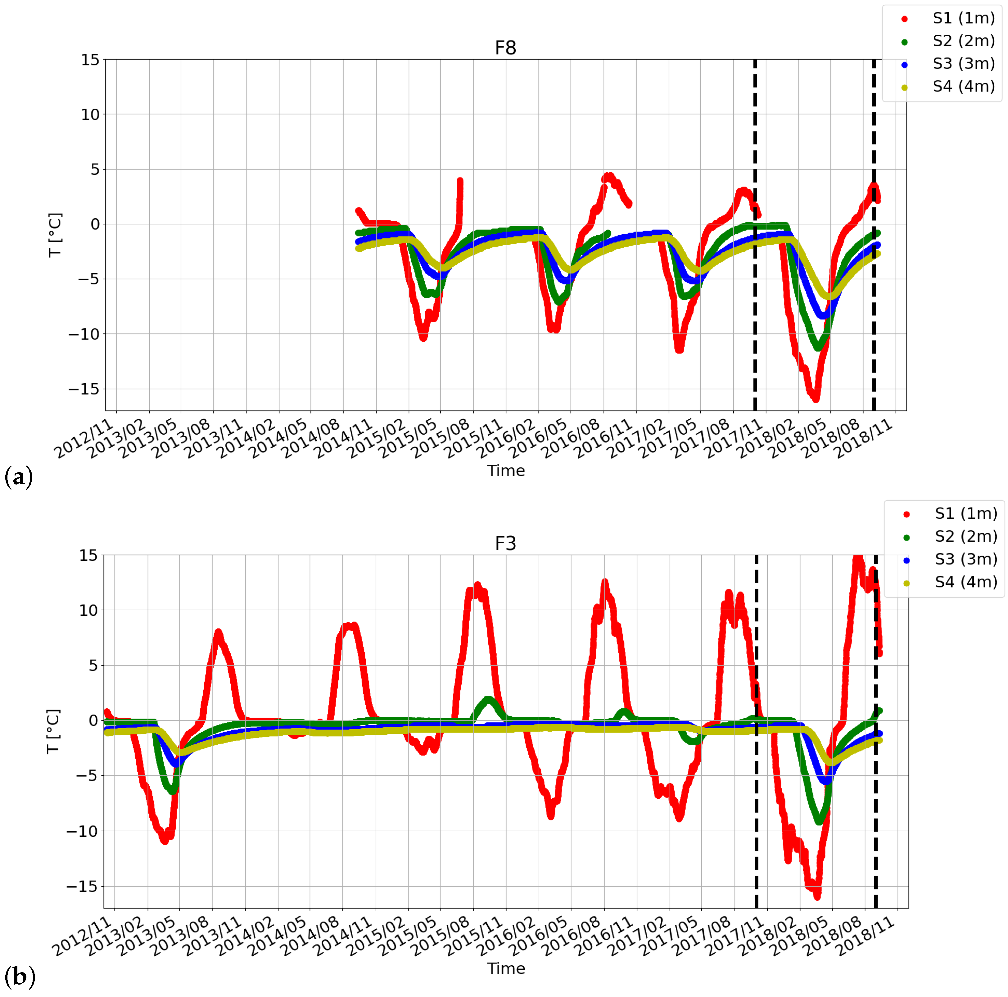
3.1. Long-Term Monitoring Temperature and Point-Scale Subsurface Measurements
3.2. UAV Imagery Acquisitions and Reconstructions
3.3. Heat Transfer Numerical Experiments
3.4. Ground-Penetrating Radar
3.5. Electrical Resistivity Tomography
4. Results
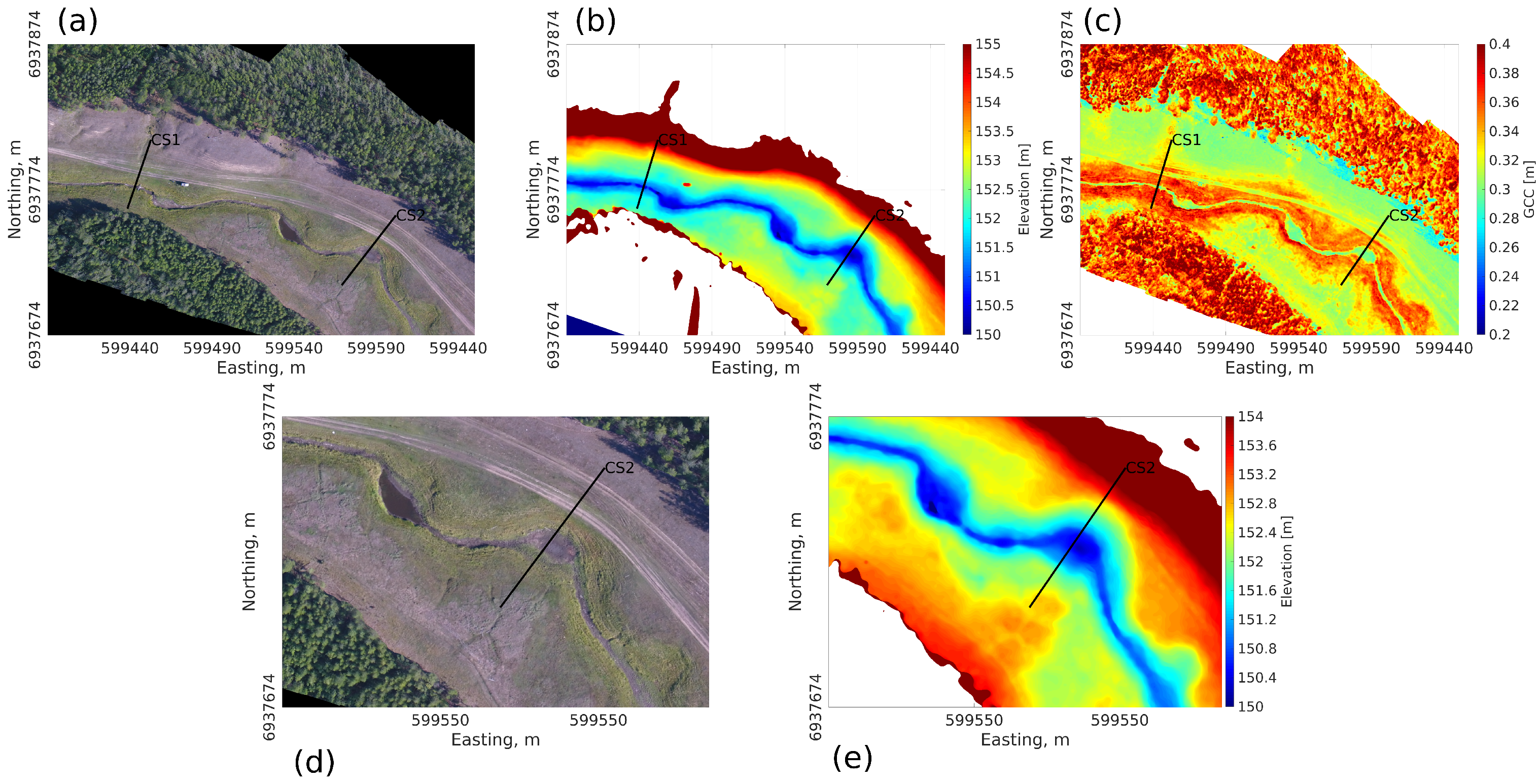
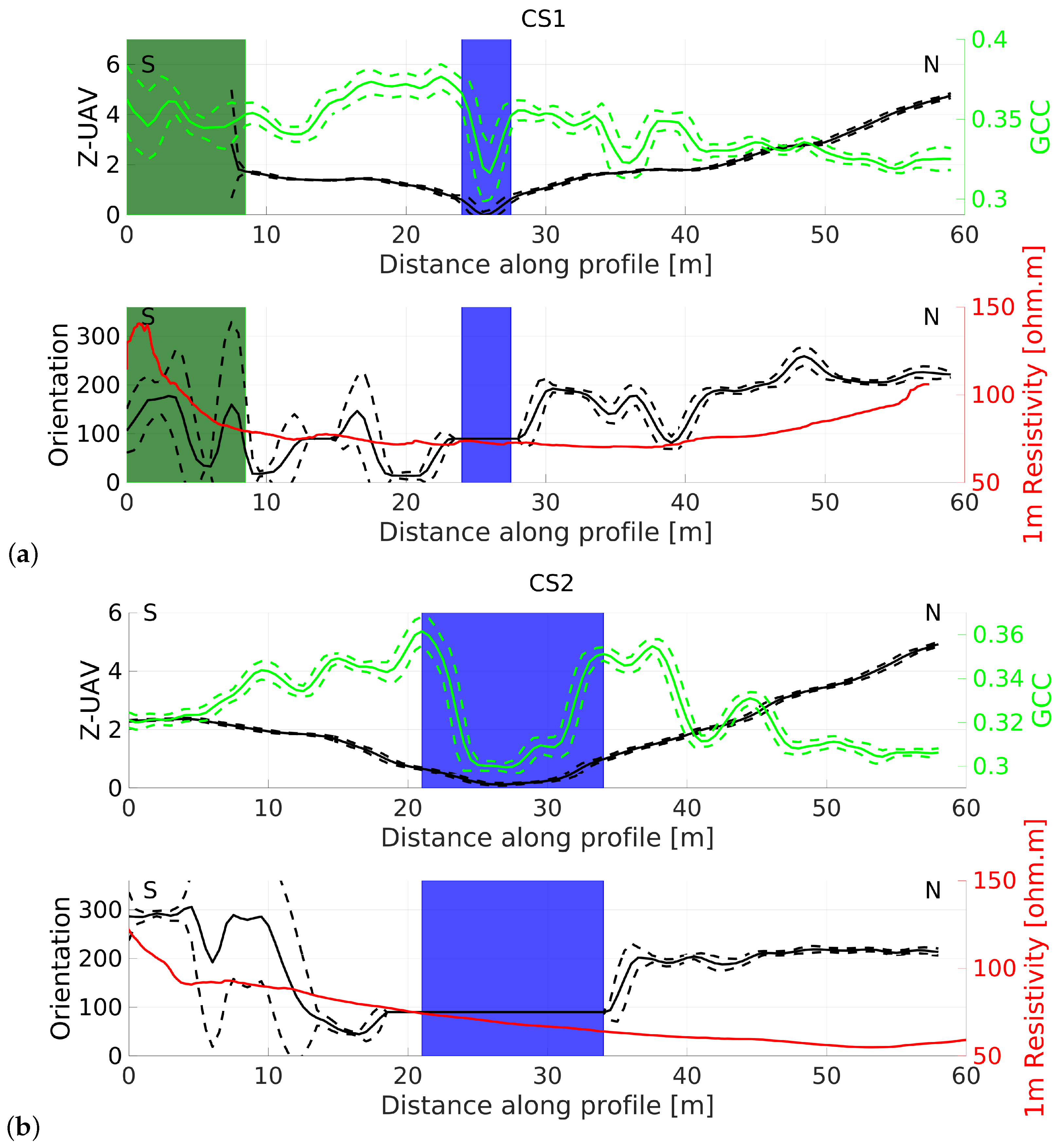
4.1. Topographic and Surface Information
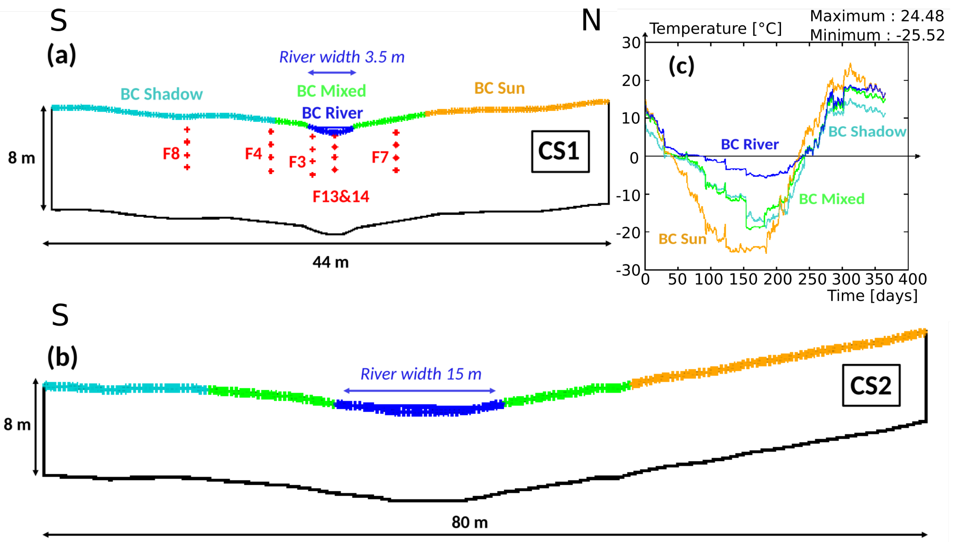
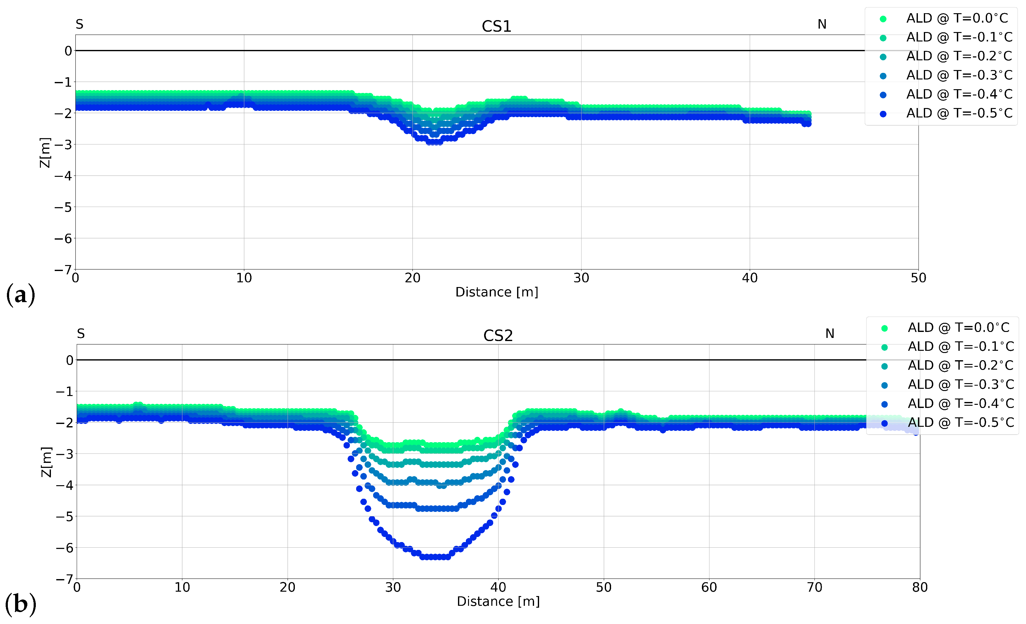
4.2. Numerical Thermal Modeling
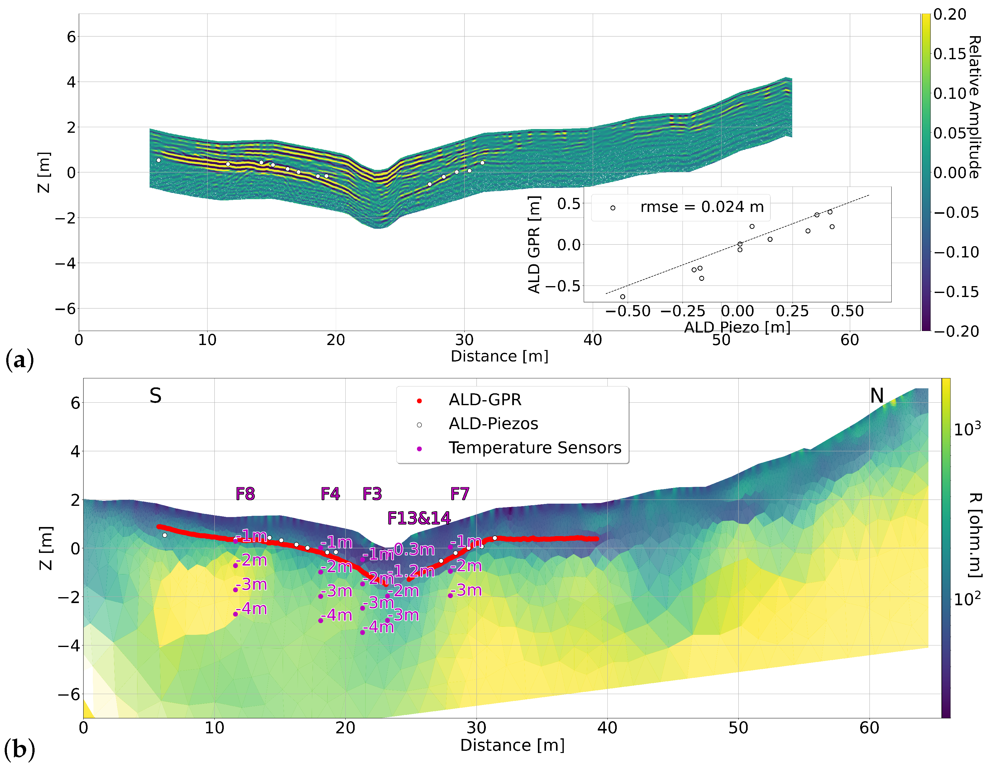
4.3. GPR Field Data on CS1 Transect
4.4. Electrical Resistivity Tomography
4.4.1. Transect CS1
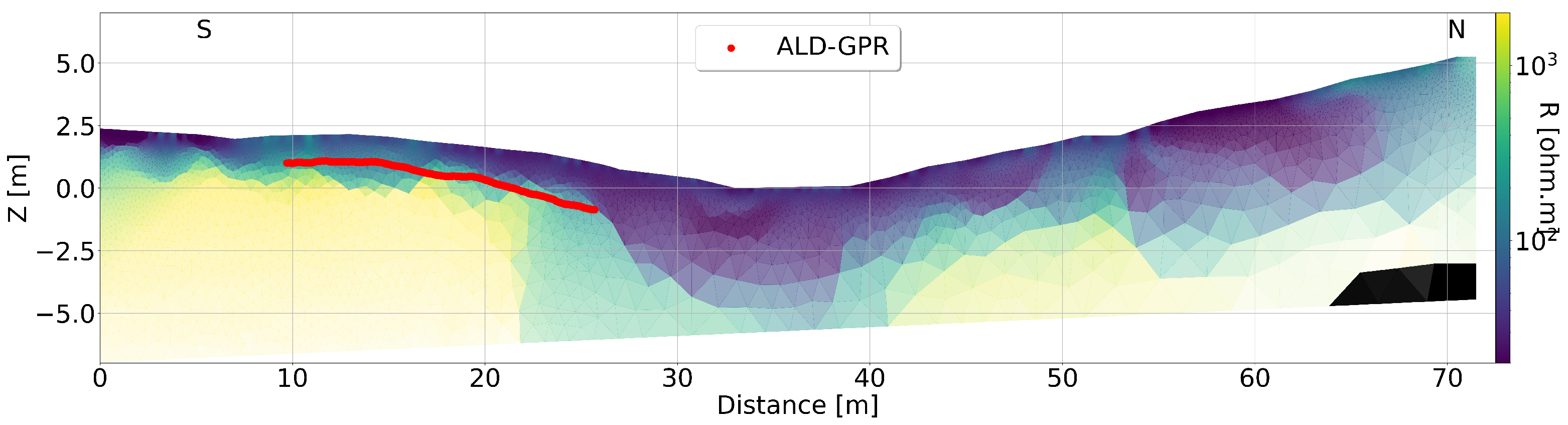
4.4.2. Transect CS2
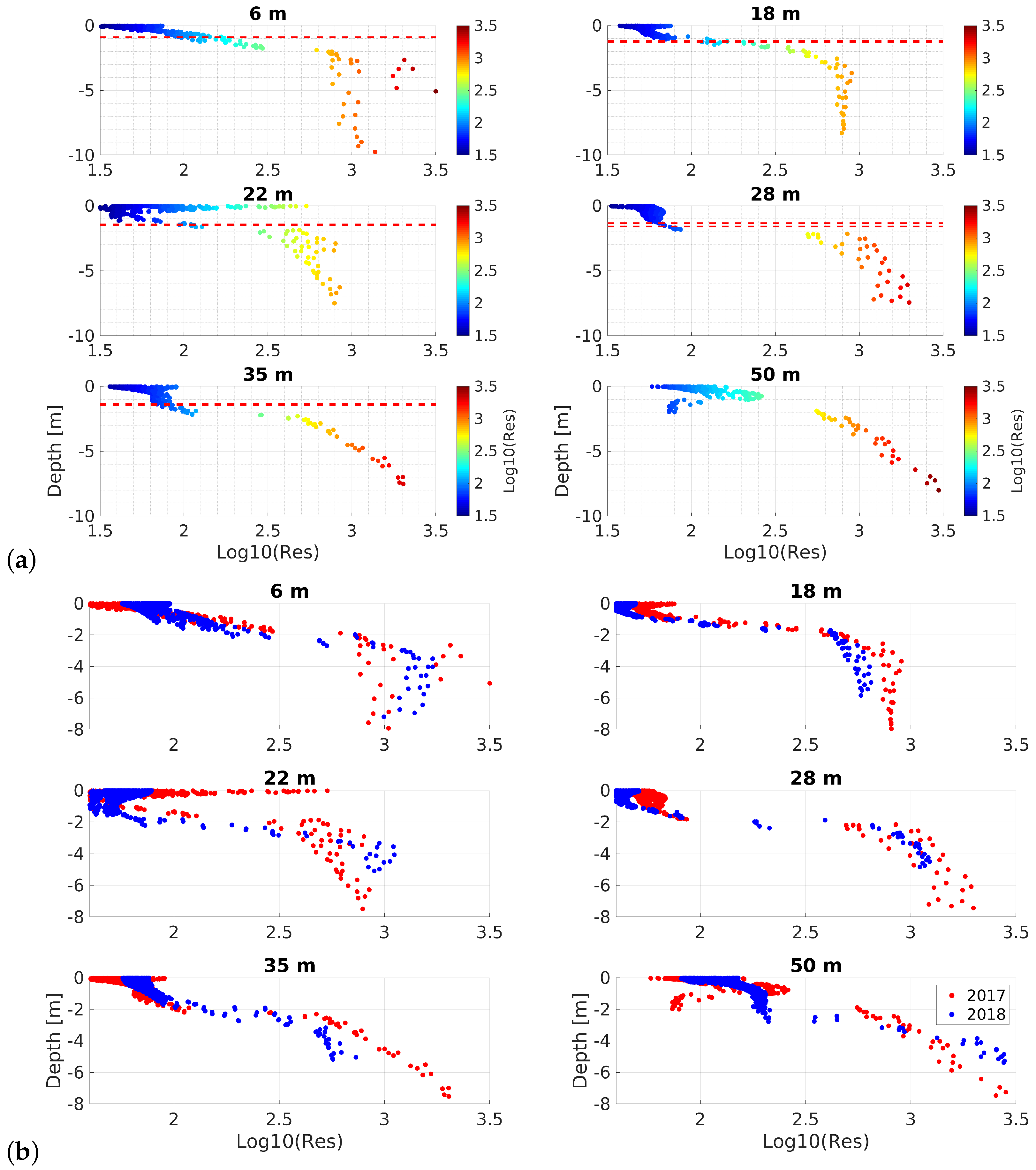
4.5. GPR and Electrical Resistivity Vertical Profile Variations
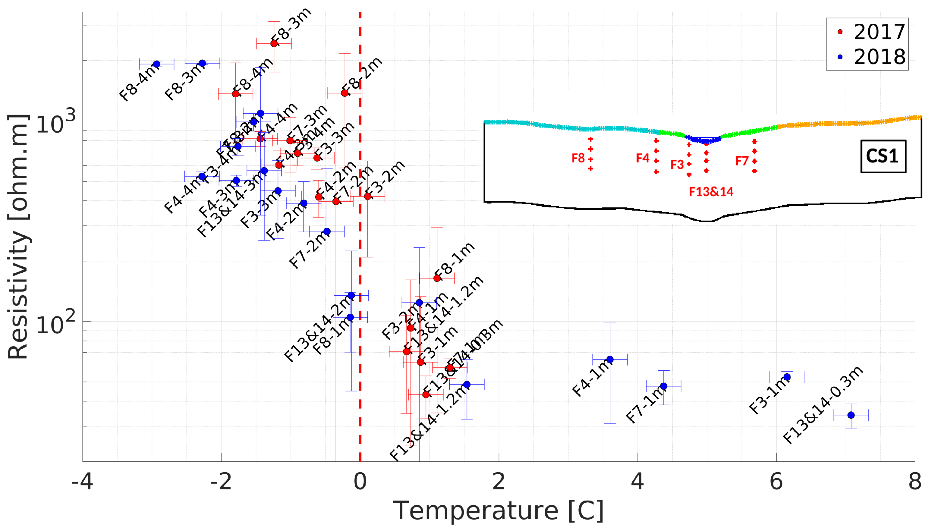
4.6. Relationship between Electrical Resistivity and Temperature
5. Discussion
5.1. Geophysical Derived Information
5.2. Thermal Modeling versus Geophysical Information
5.3. Extending CS1 Interpretation Framework to Valley Characterization
6. Conclusions
Author Contributions
Funding
Data Availability Statement
Acknowledgments
Conflicts of Interest
References
- Working Group I. Climate Change: The IPCC Scientific Assessment; Houghton, J.T., Jenkins, G., Ephraums, J.J., Eds.; Cambridge University Press: Cambridge, UK, 1990; Volume 1, p. 990. [Google Scholar]
- Overland, J.; Dunlea, E.; Box, J.E.; Corell, R.; Forsius, M.; Kattsov, V.; Olsen, M.S.; Pawlak, J.; Reiersen, L.O.; Wang, M. The urgency of Arctic change. Polar Sci. 2019, 21, 6–13. [Google Scholar] [CrossRef]
- Previdi, M.; Smith, K.L.; Polvani, L.M. Arctic amplification of climate change: A review of underlying mechanisms. Environ. Res. Lett. 2021, 16, 093003. [Google Scholar] [CrossRef]
- Serreze, M.; Barrett, A.; Stroeve, J.; Kindig, D.; Holland, M. The emergence of surface-based Arctic amplification. Cryosphere 2009, 3, 11–19. [Google Scholar] [CrossRef]
- Pörtner, H.O.; Roberts, D.C.; Masson-Delmotte, V.; Zhai, P.; Tignor, M.; Poloczanska, E.; Weyer, N. The ocean and cryosphere in a changing climate. In IPCC Special Report on the Ocean and Cryosphere in a Changing Climate; Intergovernmental Panel on Climate Change: Geneva, Switzerland, 2019. [Google Scholar]
- Hjort, J.; Karjalainen, O.; Aalto, J.; Westermann, S.; Romanovsky, V.E.; Nelson, F.E.; Etzelmüller, B.; Luoto, M. Degrading permafrost puts Arctic infrastructure at risk by mid-century. Nat. Commun. 2018, 9, 5147. [Google Scholar] [CrossRef]
- Jorgenson, M.T.; Romanovsky, V.; Harden, J.; Shur, Y.; O’Donnell, J.; Schuur, E.A.; Kanevskiy, M.; Marchenko, S. Resilience and vulnerability of permafrost to climate change. Can. J. For. Res. 2010, 40, 1219–1236. [Google Scholar] [CrossRef]
- Petrone, K.; Hinzman, L.; Shibata, H.; Jones, J.; Boone, R. The influence of fire and permafrost on sub-arctic stream chemistry during storms. Hydrol. Process. Int. J. 2007, 21, 423–434. [Google Scholar] [CrossRef]
- Pithan, F.; Mauritsen, T. Arctic amplification dominated by temperature feedbacks in contemporary climate models. Nat. Geosci. 2014, 7, 181–184. [Google Scholar] [CrossRef]
- Throop, J.; Lewkowicz, A.G.; Smith, S.L. Climate and ground temperature relations at sites across the continuous and discontinuous permafrost zones, northern Canada. Can. J. Earth Sci. 2012, 49, 865–876. [Google Scholar] [CrossRef]
- Romanovsky, V.; Osterkamp, T. Effects of unfrozen water on heat and mass transport processes in the active layer and permafrost. Permafr. Periglac. Process. 2000, 11, 219–239. [Google Scholar] [CrossRef]
- Shiklomanov, N.; Nelson, F.; Streletskiy, D.; Hinkel, K.; Brown, J. The circumpolar active layer monitoring (CALM) program: Data collection, management, and dissemination strategies. In Proceedings of the Ninth International Conference on Permafrost, Fairbanks, AK, USA, 29 June–3 July 2008; Institute of Northern Engineering Fairbanks Alaska: Fairbanks, AK, USA, 2008; Volume 29, pp. 1647–1652. [Google Scholar]
- Biskaborn, B.K.; Lanckman, J.P.; Lantuit, H.; Elger, K.; Streletskiy, D.; Cable, W.; Romanovsky, V.E. The new database of the Global Terrestrial Network for Permafrost (GTN-P). Earth Syst. Sci. Data 2015, 7, 245–259. [Google Scholar] [CrossRef]
- Riseborough, D. Soil latent heat as a filter of the climate signal in permafrost. In Proceedings of the Fifth Canadian Permafrost Conference, Collection Nordicana, Quebec City, QC, Canada, 5–9 June 1990; Citeseer: Princeton, NJ, USA, 1990; Volume 54, pp. 199–205. [Google Scholar]
- Walvoord, M.A.; Kurylyk, B.L. Hydrologic Impacts of Thawing Permafrost–A Review. Vadose Zone J. 2016, 15, 1–20. [Google Scholar] [CrossRef]
- Hughes-Allen, L.; Bouchard, F.; Séjourné, A.; Fougeron, G.; Léger, E. Automated Identification of Thermokarst Lakes Using Machine Learning in the Ice-Rich Permafrost Landscape of Central Yakutia (Eastern Siberia). Remote Sens. 2023, 15, 1226. [Google Scholar] [CrossRef]
- Mackay, J.; Burn, C. The first 20 years (1978–1979 to 1998–1999) of ice-wedge growth at the Illisarvik experimental drained lake site, western Arctic coast, Canada. Can. J. Earth Sci. 2002, 39, 95–111. [Google Scholar] [CrossRef]
- Yoshikawa, K.; Hinzman, L.D. Shrinking thermokarst ponds and groundwater dynamics in discontinuous permafrost near Council, Alaska. Permafr. Periglac. Process. 2003, 14, 151–160. [Google Scholar] [CrossRef]
- Jorgenson, M.T.; Shur, Y. Evolution of lakes and basins in northern Alaska and discussion of the thaw lake cycle. J. Geophys. Res. Earth Surf. 2007, 112. [Google Scholar] [CrossRef]
- Plug, L.J.; West, J. Thaw lake expansion in a two-dimensional coupled model of heat transfer, thaw subsidence, and mass movement. J. Geophys. Res. Earth Surf. 2009, 114. [Google Scholar] [CrossRef]
- Rowland, J.C.; Travis, B.J.; Wilson, C.J. The role of advective heat transport in talik development beneath lakes and ponds in discontinuous permafrost. Geophys. Res. Lett. 2011, 38. [Google Scholar] [CrossRef]
- Kurylyk, B.L.; MacQuarrie, K.T.; McKenzie, J.M. Climate change impacts on groundwater and soil temperatures in cold and temperate regions: Implications, mathematical theory, and emerging simulation tools. Earth Sci. Rev. 2014, 138, 313–334. [Google Scholar] [CrossRef]
- Johansson, E.; Gustafsson, L.G.; Berglund, S.; Lindborg, T.; Selroos, J.O.; Liljedahl, L.C.; Destouni, G. Data evaluation and numerical modeling of hydrological interactions between active layer, lake and talik in a permafrost catchment, Western Greenland. J. Hydrol. 2015, 527, 688–703. [Google Scholar] [CrossRef]
- Lemieux, J.M.; Fortier, R.; Talbot-Poulin, M.C.; Molson, J.; Therrien, R.; Ouellet, M.; Banville, D.; Cochand, M.; Murray, R. Groundwater occurrence in cold environments: Examples from Nunavik, Canada. Hydrogeol. J. 2016, 24, 1497–1513. [Google Scholar] [CrossRef]
- Woo, M.k. Permafrost Hydrology; Springer Science & Business Media: Berlin/Heidelberg, Germany, 2012. [Google Scholar]
- Costard, F.; Dupeyrat, L.; Gautier, E.; Carey-Gailhardis, E. Fluvial thermal erosion investigations along a rapidly eroding river bank: Application to the Lena River (central Siberia). Earth Surf. Process. Landforms J. Br. Geomorphol. Res. Group 2003, 28, 1349–1359. [Google Scholar] [CrossRef]
- Costard, F.; Gautier, E.; Konstantinov, P.; Bouchard, F.; Séjourné, A.; Dupeyrat, L.; Fedorov, A. Thermal regime variability of islands in the Lena River near Yakutsk, eastern Siberia. Permafr. Periglac. Process. 2022, 33, 18–31. [Google Scholar] [CrossRef]
- Gautier, E.; Dépret, T.; Costard, F.; Virmoux, C.; Fedorov, A.; Grancher, D.; Konstantinov, P.; Brunstein, D. Going with the flow: Hydrologic response of middle Lena River (Siberia) to the climate variability and change. J. Hydrol. 2018, 557, 475–488. [Google Scholar] [CrossRef]
- Schuur, E.A.; McGuire, A.D.; Schädel, C.; Grosse, G.; Harden, J.W.; Hayes, D.J.; Hugelius, G.; Koven, C.D.; Kuhry, P.; Lawrence, D.M.; et al. Climate change and the permafrost carbon feedback. Nature 2015, 520, 171–179. [Google Scholar] [CrossRef]
- Vonk, J.E.; Gustafsson, Ö. Permafrost-carbon complexities. Nat. Geosci. 2013, 6, 675–676. [Google Scholar] [CrossRef]
- Crampton, C. Changes in permafrost distribution produced by a migrating river meander in the northern Yukon, Canada. Arctic 1979, 32, 148–151. [Google Scholar] [CrossRef]
- Arcone, S.A.; Chacho, E.F.; Delaney, A.J. Seasonal structure of taliks beneath arctic streams determined with ground-penetrating radar. In Proceedings of the seventh International Permafrost Conference, Yellowknife, NT, Canada, 23–27 June 1998; International Permafrost Association, Canadian National Committee: Ottawa ON, Canada, 1998; pp. 19–24. [Google Scholar]
- Mikhailov, V. Convective heat exchange between rivers and floodplain taliks. In Proceedings of the Ninth International Conference on Permafrost, Institute of Northern Engineering, University of Alaska, Fairbanks, AK, USA, 29 June–3July 2008; pp. 1215–1220. [Google Scholar]
- Brosten, T.R.; Bradford, J.H.; McNamara, J.P.; Gooseff, M.N.; Zarnetske, J.P.; Bowden, W.B.; Johnston, M.E. Estimating 3D variation in active-layer thickness beneath arctic streams using ground-penetrating radar. J. Hydrol. 2009, 373, 479–486. [Google Scholar] [CrossRef]
- Minsley, B.; Abraham, J.; Smith, B.; Cannia, J.; Voss, C.; Jorgenson, M.; Walvoord, M.; Wylie, B.; Anderson, L.; Ball, L.; et al. Airborne electromagnetic imaging of discontinuous permafrost. Geophys. Res. Lett. 2012, 39. [Google Scholar] [CrossRef]
- Liu, W.; Fortier, R.; Molson, J.; Lemieux, J.M. A conceptual model for talik dynamics and icing formation in a river floodplain in the continuous permafrost zone at Salluit, Nunavik (Quebec), Canada. Permafr. Periglac. Process. 2021, 32, 468–483. [Google Scholar] [CrossRef]
- Malenfant-Lepage, J.; Doré, G.; Ingeman-Nielsen, T.; Daniel, F. Using resistivity method to characterize water flow patterns in permafrost environment (Ilulissat, Greenland). In Proceedings of the XI. International Conference on Permafrost, Potsdam, Germany, 20–24 June 2016; p. 966. [Google Scholar]
- Roux, N.; Costard, F.; Grenier, C. Laboratory and Numerical Simulation of the Evolution of a River’s Talik. Permafr. Periglac. Process. 2017, 28, 460–469. [Google Scholar] [CrossRef]
- Grenier, C.; Anbergen, H.; Bense, V.; Chanzy, Q.; Coon, E.; Collier, N.; Costard, F.; Ferry, M.; Frampton, A.; Frederick, J.; et al. Groundwater flow and heat transport for systems undergoing freeze-thaw: Intercomparison of numerical simulators for 2D test cases. Adv. Water Resour. 2018, 114, 196–218. [Google Scholar] [CrossRef]
- Uhlemann, S.; Dafflon, B.; Peterson, J.; Ulrich, C.; Shirley, I.; Michail, S.; Hubbard, S. Geophysical Monitoring Shows that Spatial Heterogeneity in Thermohydrological Dynamics Reshapes a Transitional Permafrost System. Geophys. Res. Lett. 2021, 48, e2020GL091149. [Google Scholar] [CrossRef]
- Jafarov, E.E.; Harp, D.R.; Coon, E.T.; Dafflon, B.; Tran, A.P.; Atchley, A.L.; Lin, Y.; Wilson, C.J. Estimation of subsurface porosities and thermal conductivities of polygonal tundra by coupled inversion of electrical resistivity, temperature, and moisture content data. Cryosphere 2020, 14, 77–91. [Google Scholar] [CrossRef]
- Tran, A.P.; Dafflon, B.; Bisht, G.; Hubbard, S.S. Spatial and temporal variations of thaw layer thickness and its controlling factors identified using time-lapse electrical resistivity tomography and hydro-thermal modeling. J. Hydrol. 2018, 561, 751–763. [Google Scholar] [CrossRef]
- Léger, E.; Dafflon, B.; Robert, Y.; Ulrich, C.; Peterson, J.; Biraud, S.; Romanovsky, V.; Hubbard, S. A distributed temperature profiling method for assessing spatial variability of ground temperatures in a discontinuous permafrost region of Alaska. Cryosphere 2019, 13, 2853–2867. [Google Scholar] [CrossRef]
- Léger, E.; Saintenoy, A.; Serhir, M.; Costard, F.; Grenier, C. Brief Communication: Monitoring active layer dynamic using a lightweight nimble Ground-Penetrating Radar system. A laboratory analog test case. Cryosphere Discuss. 2022, 17, 1271–1277. [Google Scholar] [CrossRef]
- Wielandt, S.; Uhlemann, S.; Fiolleau, S.; Dafflon, B. Low-Power, Flexible Sensor Arrays with Solderless Board-to-Board Connectors for Monitoring Soil Deformation and Temperature. Sensors 2022, 22, 2814. [Google Scholar] [CrossRef]
- Dafflon, B.; Wielandt, S.; Lamb, J.; McClure, P.; Shirley, I.; Uhlemann, S.; Wang, C.; Fiolleau, S.; Brunetti, C.; Akins, F.H.; et al. A Distributed Temperature Profiling System for Vertically and Laterally Dense Acquisition of Soil and Snow Temperature. Cryosphere 2022, 16, 719–736. [Google Scholar] [CrossRef]
- Majdański, M.; Dobiński, W.; Marciniak, A.; Owoc, B.; Glazer, M.; Osuch, M.; Wawrzyniak, T. Variations of permafrost under freezing and thawing conditions in the coastal catchment Fuglebekken (Hornsund, Spitsbergen, Svalbard). Permafr. Periglac. Process. 2022, 33, 264–276. [Google Scholar] [CrossRef]
- McClymont, A.F.; Hayashi, M.; Bentley, L.R.; Christensen, B.S. Geophysical imaging and thermal modeling of subsurface morphology and thaw evolution of discontinuous permafrost. J. Geophys. Res. Earth Surf. 2013, 118, 1826–1837. [Google Scholar] [CrossRef]
- Jepsen, S.; Voss, C.; Walvoord, M.; Rose, J.; Minsley, B.; Smith, B. Sensitivity analysis of lake mass balance in discontinuous permafrost: The example of disappearing Twelvemile Lake, Yukon Flats, Alaska (USA). Hydrogeol. J. 2012, 21, 185–200. [Google Scholar] [CrossRef]
- Fedorov, A.; Gavriliev, P.; Konstantinov, P.Y.; Hiyama, T.; Iijima, Y.; Iwahana, G. Estimating the water balance of a thermokarst lake in the middle of the Lena River basin, eastern Siberia. Ecohydrology 2014, 7, 188–196. [Google Scholar] [CrossRef]
- Soloviev, P. Alass thermokarst relief of Central Yakutia. In Proceedings of the International Permafrost Conference, Yakutsk, Russia, 13–28 July 1973; Volume 2. [Google Scholar]
- Desyatkin, R.; Filippov, N.; Desyatkin, A.; Konyushkov, D.; Goryachkin, S. Degradation of arable soils in central Yakutia: Negative consequences of global warming for yedoma landscapes. Front. Earth Sci. 2021, 9, 683730. [Google Scholar] [CrossRef]
- Hughes-Allen, L.; Bouchard, F.; Laurion, I.; Séjourné, A.; Marlin, C.; Hatté, C.; Costard, F.; Fedorov, A.; Desyatkin, A. Seasonal patterns in greenhouse gas emissions from thermokarst lakes in Central Yakutia (Eastern Siberia). Limnol. Oceanogr. 2021, 66, S98–S116. [Google Scholar] [CrossRef]
- Hughes-Allen, L.; Bouchard, F.; Hatté, C.; Meyer, H.; Pestryakova, L.A.; Diekmann, B.; Subetto, D.A.; Biskaborn, B.K. 14,000-year Carbon Accumulation Dynamics in a Siberian Lake Reveal Catchment and Lake Productivity Changes. Front. Earth Sci. 2021, 9, 949116. [Google Scholar] [CrossRef]
- Gidrometeoizdat. Handbook on the USSR Climate. Series 3 Long-Term Data. Part 1–6; Book 1; Technical Report; Gidrometeoizdat: Leningrad, Russia, 1989; Volume 24. [Google Scholar]
- Gavrilova, M. Climate of Central Yakutia; Yakutknogoizdat: Yakutsk, Russia, 1973; p. 120. (In Russian) [Google Scholar]
- Schirrmeister, L.; Froese, D.; Tumskoy, V.; Grosse, G.; Wetterich, S. Yedoma: Late Pleistocene ice-rich syngenetic permafrost of Beringia. In Encyclopedia of Quaternary Science, 2nd ed.; Elsevier: Amsterdam, The Netherlands, 2013; pp. 542–552. [Google Scholar]
- Hugelius, G.; Strauss, J.; Zubrzycki, S.; Harden, J.W.; Schuur, E.; Ping, C.L.; Schirrmeister, L.; Grosse, G.; Michaelson, G.J.; Koven, C.D.; et al. Estimated stocks of circumpolar permafrost carbon with quantified uncertainty ranges and identified data gaps. Biogeosciences 2014, 11, 6573–6593. [Google Scholar] [CrossRef]
- Ulrich, M.; Wetterich, S.; Rudaya, N.; Frolova, L.; Schmidt, J.; Siegert, C.; Fedorov, A.N.; Zielhofer, C. Rapid thermokarst evolution during the mid-Holocene in Central Yakutia, Russia. Holocene 2017, 27, 1899–1913. [Google Scholar] [CrossRef]
- Konstantinov, P.; Fedorov, A.; Machimura, T.; Iwahana, G.; Yabuki, H.; Iijima, Y.; Costard, F. Use of automated recorders (data loggers) in permafrost temperature monitoring. Earth Cryosphere 2011, 15, 23–32. [Google Scholar]
- Chen, C.; Jia, Y.; Chen, Y.; Mehmood, I.; Fang, Y.; Wang, G. Nitrogen isotopic composition of plants and soil in an arid mountainous terrain: South slope versus north slope. Biogeosciences 2018, 15, 369–377. [Google Scholar] [CrossRef]
- Gindraux, S.; Boesch, R.; Farinotti, D. Accuracy Assessment of Digital Surface Models from Unmanned Aerial Vehicles’ Imagery on Glaciers. Remote Sens. 2017, 9, 186. [Google Scholar] [CrossRef]
- Dafflon, B.; Oktem, R.; Peterson, J.; Ulrich, C.; Tran, A.P.; Romanovsky, V.; Hubbard, S.S. Coincident aboveground and belowground autonomous monitoring to quantify covariability in permafrost, soil, and vegetation properties in Arctic tundra. J. Geophys. Res. Biogeosciences 2017, 122, 1321–1342. [Google Scholar] [CrossRef]
- Barnes, R. RichDEM: Terrain Analysis Software; RichDEM: Yorkshire, UK, 2016. [Google Scholar]
- Huete, A. Huete, AR A soil-adjusted vegetation index (SAVI). Remote Sensing of Environment. Remote Sens. Environ. 1988, 25, 295–309. [Google Scholar] [CrossRef]
- Falco, N.; Wainwright, H.M.; Dafflon, B.; Ulrich, C.; Soom, F.; Peterson, J.E.; Brown, J.B.; Schaettle, K.B.; Williamson, M.; Cothren, J.D.; et al. Influence of soil heterogeneity on soybean plant development and crop yield evaluated using time-series of UAV and ground-based geophysical imagery. Sci. Rep. 2021, 11, 7046. [Google Scholar] [CrossRef]
- Stolt, R.H. Migration by Fourier transform. Geophysics 1978, 43, 23–48. [Google Scholar] [CrossRef]
- Stockwell, J.W., Jr. The CWP/SU: Seismic Un * x package. Comput. Geosci. 1999, 25, 415–419. [Google Scholar] [CrossRef]
- Rücker, T.G.C.; Spitzer, K. 3-d modeling and inversion of DC resistivity data incorporating topography–Part II: Inversion. Geophys. J. Int. 2006, 166, 506–517. [Google Scholar] [CrossRef]
- Rücker, C.; Günther, T.; Spitzer, K. 3-D modeling and inversion of DC resistivity data incorporating topography–Part I: Modeling. Geophys. J. Int. 2006, 166, 495–505. [Google Scholar] [CrossRef]
- Geuzaine, C.; Remacle, J.F. Gmsh: A 3-D finite element mesh generator with built-in pre-and post-processing facilities. Int. J. Numer. Methods Eng. 2009, 79, 1309–1331. [Google Scholar] [CrossRef]
- Windirsch, T.; Grosse, G.; Ulrich, M.; Schirrmeister, L.; Fedorov, A.N.; Konstantinov, P.Y.; Fuchs, M.; Jongejans, L.L.; Wolter, J.; Opel, T.; et al. Organic carbon characteristics in ice-rich permafrost in alas and Yedoma deposits, central Yakutia, Siberia. Biogeosciences 2020, 17, 3797–3814. [Google Scholar] [CrossRef]
- Archie, G. The electrical resistivity log as an aid in determining some reservoir characteristics. Trans. Am. Inst. Min. Mettallurgical Eng. 1942, 146, 54–61. [Google Scholar] [CrossRef]
- Hauck, C. Frozen ground monitoring using DC resistivity tomography. Geophys. Res. Lett. 2002, 29, 12-1–12-4. [Google Scholar] [CrossRef]
- Nakao, K.; McGinnis, L.; Clark, C. Geophysical identification of frozen and unfrozen ground, Antarctica. In Proceedings of the Permafrost: North American Contribution [to The] Second International Conference, Yakutsk, Russia, 13–28 July 1973; National Academies: Washington, DC, USA, 1973; Volume 2, p. 136. [Google Scholar]
- Clément, R.; Descloitres, M.; Günther, T.; Ribolzi, O.; Legchenko, A. Influence of shallow infiltration on time-lapse ERT: Experience of advanced interpretation. Comptes Rendus Geosci. 2009, 341, 886–898. [Google Scholar] [CrossRef]
- Costard, F.; Dupeyrat, L.; Séjourné, A.; Bouchard, F.; Fedorov, A.; Saint-Bézar, B. Retrogressive Thaw Slumps on Ice-Rich Permafrost Under Degradation: Results From a Large-Scale Laboratory Simulation. Geophys. Res. Lett. 2021, 48, e2020GL091070. [Google Scholar] [CrossRef]


Disclaimer/Publisher’s Note: The statements, opinions and data contained in all publications are solely those of the individual author(s) and contributor(s) and not of MDPI and/or the editor(s). MDPI and/or the editor(s) disclaim responsibility for any injury to people or property resulting from any ideas, methods, instructions or products referred to in the content. |
© 2023 by the authors. Licensee MDPI, Basel, Switzerland. This article is an open access article distributed under the terms and conditions of the Creative Commons Attribution (CC BY) license (https://creativecommons.org/licenses/by/4.0/).
Share and Cite
Léger, E.; Saintenoy, A.; Grenier, C.; Séjourné, A.; Pohl, E.; Bouchard, F.; Pessel, M.; Bazhin, K.; Danilov, K.; Costard, F.; et al. Comparing Thermal Regime Stages along a Small Yakutian Fluvial Valley with Point Scale Measurements, Thermal Modeling, and Near Surface Geophysics. Remote Sens. 2023, 15, 2524. https://doi.org/10.3390/rs15102524
Léger E, Saintenoy A, Grenier C, Séjourné A, Pohl E, Bouchard F, Pessel M, Bazhin K, Danilov K, Costard F, et al. Comparing Thermal Regime Stages along a Small Yakutian Fluvial Valley with Point Scale Measurements, Thermal Modeling, and Near Surface Geophysics. Remote Sensing. 2023; 15(10):2524. https://doi.org/10.3390/rs15102524
Chicago/Turabian StyleLéger, Emmanuel, Albane Saintenoy, Christophe Grenier, Antoine Séjourné, Eric Pohl, Frédéric Bouchard, Marc Pessel, Kirill Bazhin, Kencheeri Danilov, François Costard, and et al. 2023. "Comparing Thermal Regime Stages along a Small Yakutian Fluvial Valley with Point Scale Measurements, Thermal Modeling, and Near Surface Geophysics" Remote Sensing 15, no. 10: 2524. https://doi.org/10.3390/rs15102524