Article

Investigating Foliar Macro- and Micronutrient Variation with Chlorophyll Fluorescence and Reflectance Measurements at the Leaf and Canopy Scales in Potato

1
Optics of Photosynthesis Laboratory, Institute for Atmospheric and Earth System Research/Forest Sciences and Viikki Plant Science Center, University of Helsinki, 00014 Helsinki, Finland
2
Plant Phenomics Research Centre, Academy for Advanced Interdisciplinary Studies, Nanjing Agricultural University, No. 1 Weigang, Xuanwu District, Nanjing 210095, China
3
Department of Remote Sensing and Photogrammetry, Finnish Geospatial Research Institute, National Land Survey of Finland, Vuorimiehentie 5, 02150 Espoo, Finland
*
Author to whom correspondence should be addressed.
Remote Sens. 2023, 15(10), 2498; https://doi.org/10.3390/rs15102498
Submission received: 15 March 2023 / Revised: 21 April 2023 / Accepted: 3 May 2023 / Published: 9 May 2023
(This article belongs to the Special Issue Remote Sensing for Crop Nutrients and Related Traits)

Abstract

:
Vegetation indices (VIs) related to plant greenness have been studied extensively for the remote detection of foliar nitrogen content. Yet, the potential of chlorophyll fluorescence (ChlF) and photoprotection-based indices such as the photochemical reflectance index (PRI) or the chlorophyll/carotenoid index (CCI) for the detection of a wide range of nutrients remains elusive. We measured the dynamics of foliar macro- and micronutrient contents in potato plants as affected by fertilization and water stress, along with leaf and canopy level observations of spectral reflectance and ChlF (or solar-induced fluorescence). ChlF and photoprotection-related indices were more strongly related to a wide range of foliar nutrient contents compared to greenness-based indices. At the leaf level, relationships were largely mediated by foliar chlorophyll contents (Cab) and leaf morphology, which resulted in two contrasting groupings: a group dominated by macronutrients N, P, K, and Mg that decreased during canopy development and was positively correlated with Cab, and a group including Cu, Mn, Zn, and S that increased and was negatively related to Cab. At the canopy-level, spectral indices were additionally influenced by canopy structure, and so their capacity to detect foliar nutrient contents depends on the spatiotemporal covariation between foliar Cab, morphology, and canopy structure within the observations.

1. Introduction

Population growth over the last century has resulted in increased agricultural activity and the use of chemical fertilizers. While fertilization of food crops brings with it larger yields, excess fertilization not only costs the farmer money, but also carries considerable environmental risks caused by eutrophication through the leaching of nutrients into groundwater and waterways [1]. Precision agriculture methods, including the gathering of near-real-time optical data from crops, answer the need for farmers to optimize the application of fertilizers [2,3]. However, the applicability of optical methods to detect plant nutrient contents has mostly concentrated on the use of simple vegetation indices (VIs) related to chlorophyll contents and therefore canopy greenness to track nitrogen contents [4]. The potential of emerging optical signals, related to plant photoprotection strategies or chlorophyll fluorescence, for tracking a wider range of nutrients remains poorly understood.
The essential nutrients needed by plants are divided into macro- and micronutrients, depending on the amount of nutrient that is required by a plant. Nitrogen (N) is the most common plant growth-limiting macronutrient and an estimated 1–5% of above-ground plant dry matter is N, making it the second most needed element after carbon (C) [5]. In plants, N is used, for example, to produce chlorophyll, nucleic acids, and proteins, such as ribulose-1,5-bisphosphate carboxylase/oxygenase (RuBisCO) [6], which is used by plants in carbon fixation. Other macronutrients include phosphorus (P), sulfur (S), calcium (Ca), magnesium (Mg), and potassium (K). Micronutrients, such as copper (Cu), iron (Fe), manganese (Mn), and zinc (Zn) play varying important roles in plant protein formation and plant stress response [5] (Table 1).
Plants require a balanced amount of macro- and micronutrients to function optimally. A deficiency of mineral nutrients can lead to a decrease in the overall photosynthetic activity of foliage [7,8] and reduced plant growth [9], affecting canopy development by reducing the leaf area index (LAI) of the canopy [10]. Accordingly, nutrient deficiencies are expected to express themselves through optical signatures both at the leaf, e.g., via pigment contents and radiation absorption, and at canopy levels, via structural effects such as a decrease in leaf area, offering opportunities for the remote detection of plant nutrient dynamics using optical remote sensing techniques.
Vegetation indices (VIs) derived from leaf reflectance have been used in remote sensing since at least the 1960s, the most well-known of which is the normalized difference vegetation index (NDVI) [11], based on the red, which is absorbed by the vegetation, and near-infrared, which is strongly reflected by the vegetation, reflectance difference. Originally used for differentiating vegetated areas from non-vegetated areas in satellite data [12], it has since seen use in both commercial and scientific applications [4] and has been used to detect N from crops [13,14]. It does, however, suffer from limitations due to saturation under high canopy cover conditions [12,15,16].
Additional vegetation greenness-based indices (henceforth referred to as greenness indices in this study together with NDVI) have been developed to refine the original NDVI formulation, such as the MERIS terrestrial chlorophyll index (MTCI) [17]. The MTCI is a proxy for the position of the red edge, which is the sharp increase in vegetation reflectance between the red and near-infrared that shifts towards longer wavelengths with increasing chlorophyll contents. While susceptible to soil background effects at early growth stages [18], MTCI has been used for canopy chlorophyll [17] and N [18,19,20] estimation on various plant species, while other related red edge indices have been shown to correlate with canopy N status in grasslands and potato fields [21]. These approaches are complementary to studies that make use of absorption features in the short-wave infrared (SWIR) region of the spectrum that relate to N containing proteins [22,23].
Recent technological advances in both uncrewed aerial vehicles (UAVs) and field spectroscopy offer new opportunities for optical remote sensing in precision agriculture at increased spectral, spatial, and temporal resolution [24,25]. A range of spectral indices are available that do not only relate to plant greenness, but also capture plant photoprotective dynamics and are thus potentially sensitive to both long-term and short-term impacts of nutrient deficits. In contrast to indices based solely on plant greenness which are not sensitive to rapid physiological adjustments in plants, the emission of chlorophyll fluorescence (ChlF), measurable at the canopy level in terms of solar induced fluorescence, SIF [26,27,28], is directly and instantaneously related to both photosynthetic light absorption and photoprotection [29]. Likewise, the photoprotection-sensitive and carotenoid-dependent indices photochemical reflectance index (PRI) [30] and chlorophyll/carotenoid index (CCI) [31] (which in this study are referred to as photoprotection indices), could also provide new opportunities to capture the optical expression of plant stress (e.g., nutrient deficiency) across scales [32].
ChlF is electromagnetic radiation emitted by chlorophyll molecules when exposed to photosynthetically active radiation (PAR). The intensity of the ChlF signal is dependent on the fraction of absorbed PAR (fAPAR) absorbed by the leaf and related to its chlorophyll content, as well as the fluorescence quantum yield, which is connected to the regulation of the photosynthetic machinery [27,29,33]. ChlF is emitted from the leaf between 650 nm and 850 nm, and it has two peaks, at around 685 nm (the red peak) and 740 nm (far-red peak). In turn, the shape of the ChlF spectra has been shown to be strongly dependent on the leaf chlorophyll (Cab) content, which mediates the predominant reabsorption of red ChlF relative to far-red ChlF photons both at the leaf and canopy scales [34,35,36,37], affecting the ratio of the red to far-red peaks. At the canopy scale, the SIF signal is influenced by both scattering and re-absorption from the canopy [37]. Since ChlF is one of the three alternative pathways for the utilization of absorbed excitation energy in the leaf, ChlF carries information on the dynamics of the other two pathways: photochemistry leading to photosynthesis and non-photochemical quenching (NPQ) related to photoprotection. The dual role of ChlF, tracking both PAR absorption (related to plant greenness) but also photoprotection and photosynthesis dynamics, makes ChlF a valuable tool in non-invasive plant stress detection [38,39] and has been shown to track canopy Gross Primary Production (GPP) [27,40].
Since the SIF signal is relatively weak compared to canopy reflected radiation, its retrieval is accomplished within Fraunhofer or Telluric absorption bands, such as the oxygen O2B and O2A-bands, located near the fluorescence peaks at circa 687 nm and 760 nm, respectively, using the Fraunhofer Line Discriminator (FLD) principle and its more advanced variants [41]. Furthermore, since the SIF-signal is only emitted by chlorophyll molecules, the signal is potentially less susceptible to non-photosynthetic background, than e.g., soil reflectance-based vegetation indices [42]. In terms of plant nutrient research, the capacity of SIF to detect foliar nutrient contents remains unclear and, to the best of our knowledge, has been limited to studies focusing on N. As such, SIF has been successfully used to estimate foliar N contents in winter wheat (Triticum aestivum) at the leaf and canopy scales [43,44], as well as in almond (Prunus dulcis) on the canopy scale [25]. However, the potential of SIF to detect a wider range of plant nutrients remains to be elucidated.
The PRI and CCI indices are optical proxies of plant carotenoid pigment contents, which are closely related to photosynthetic light use efficiency and plant photoprotection. Originally, PRI was found to correlate with the epoxidation state of the xanthophyll cycle pigments as well as photosynthetic efficiency in plants, and CCI was developed as an adaptation of PRI to measure evergreen photosynthesis at various scales [31]. PRI has been found to correlate with leaf level N dynamics in sunflower plants (Helianthus annuus) [45] and conifer seedlings [46], as well as canopy level N dynamics in several annual and perennial species [47,48].
With these photoprotection indices, N dynamics are expectedly mediated through indirect means, since N deficient plants that would suffer from lower photosynthetic rates would tend to have increased photoprotection [47], which would then be reflected by PRI and CCI. Research by Kawamura et al. [49] also showed that canopy level PRI was correlated with P contents in several pasture species. Yet, despite the intrinsic potential, the capacity of photoprotection-related indices such as PRI and CCI to investigate a wider range of foliar nutrients is yet to be explored, as are the factors underlying the relationship at the leaf and canopy scales.
The goal of this paper is to characterize the relationship between greenness and photoprotection-based vegetation indices, SIF, and the dynamics of foliar macro- and micronutrients in potato plants using both leaf- and canopy-scale observations. We hypothesize that SIF and photoprotection-related indices such as PRI and CCI will be more strongly correlated with foliar micro and macronutrient dynamics compared to vegetation indices such as the NDVI, MTCI, or red-edge, given their more direct coupling to nutrient-related physiological and PAR absorption dynamics. We test this hypothesis by combining observations across fertilization and water stress experiments in order to generate variability in terms of foliar nutrient contents, canopy development, and physiological stress. Finally, using UAV-based measurements, we investigate how the correlations between foliar nutrient contents and leaf spectral indices scale from the leaf to the canopy level, identifying the indices with stronger potential for remote sensing applications.

2. Materials and Methods

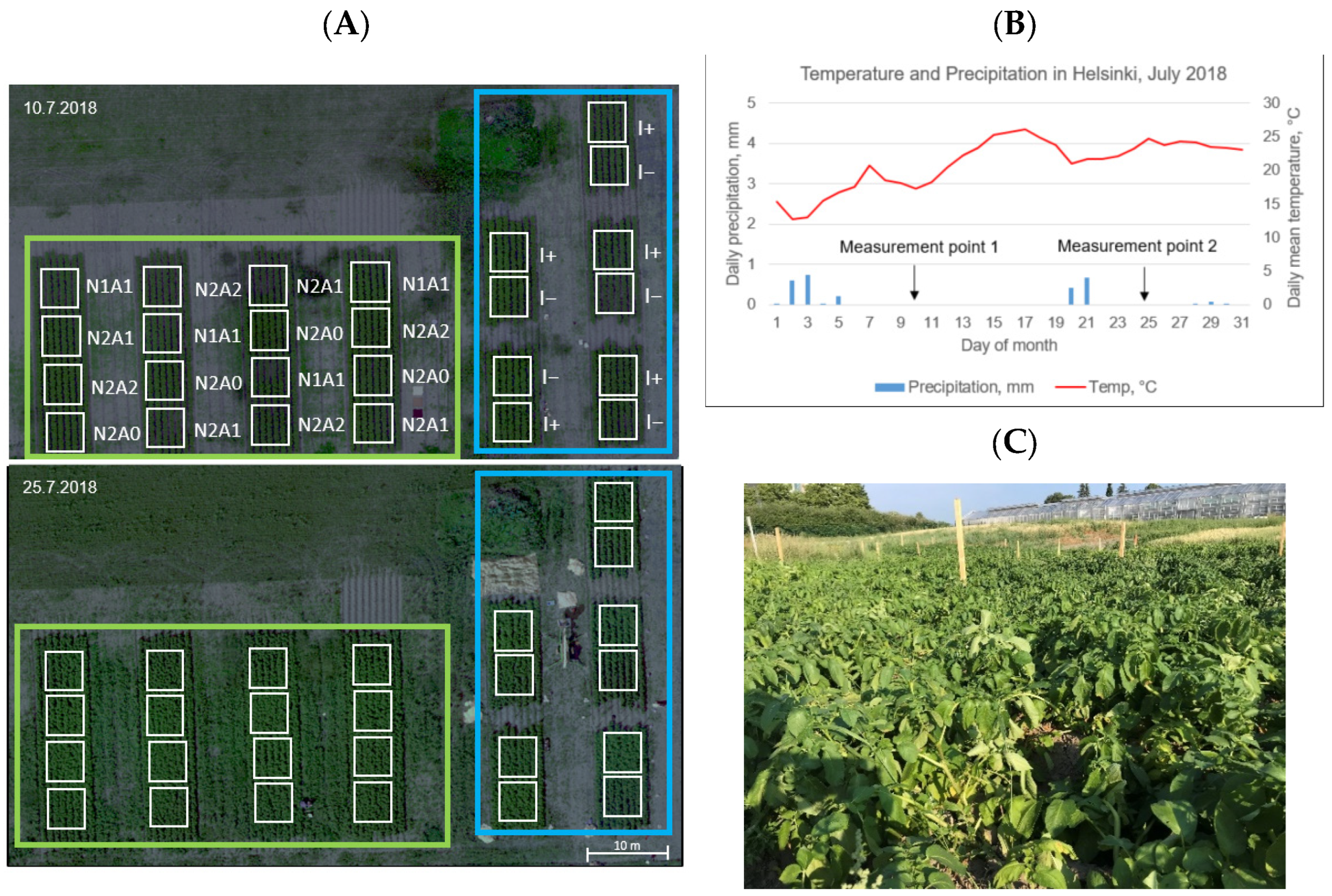
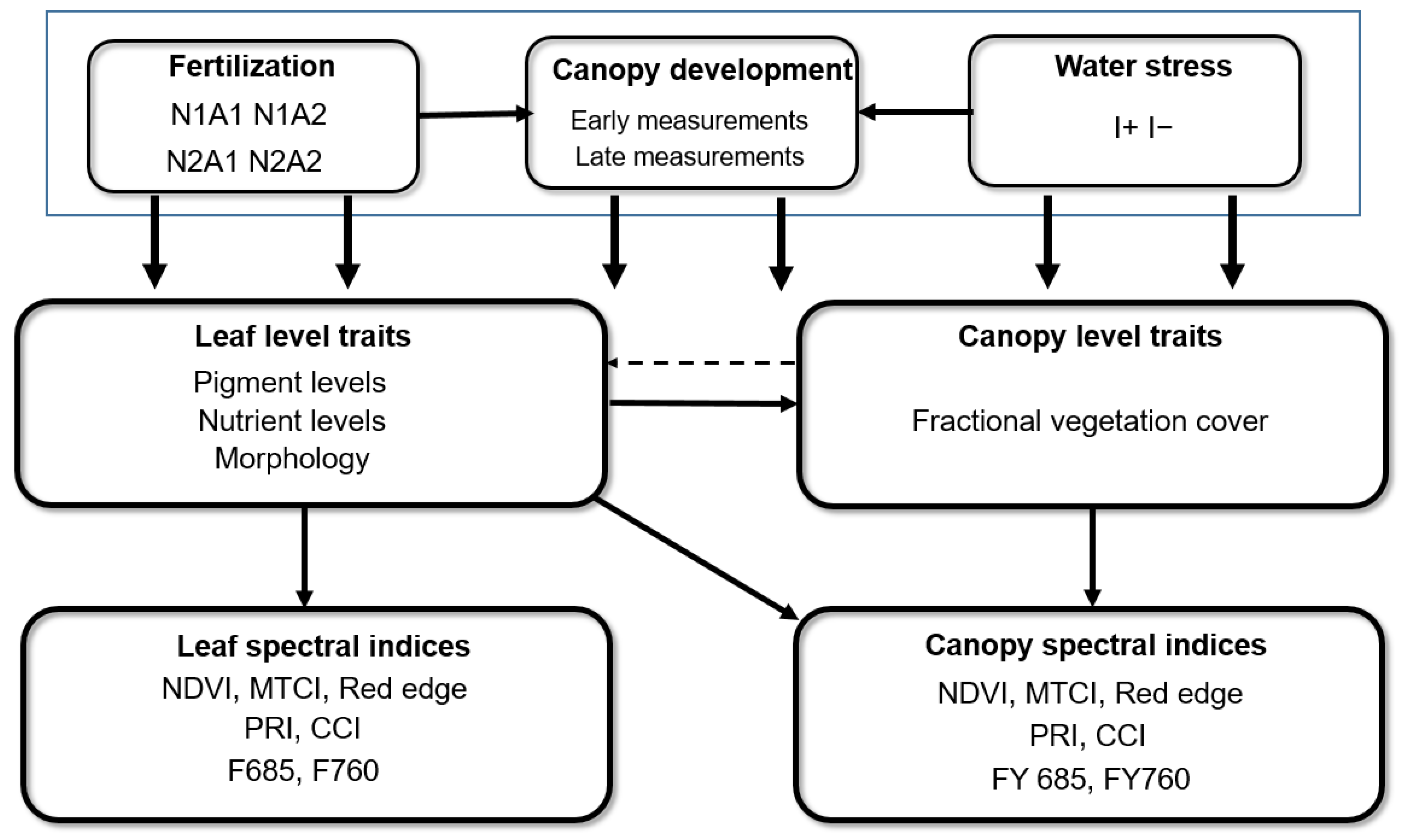
2.1. Experiment Design

Experiments were conducted during May–September of 2018 in Helsinki, Finland, on the University of Helsinki Viikki Campus (60.2269°N, 25.0186°E). Potatoes of the variety ‘Lady Felicia’ were planted at the end of May in 5 m × 5 m (see Figure 1) plots with a distance between plants of 30 cm (within row) and 70 cm (between row), with an overall density of 4000 kg/ha. The potato is an important food plant and was selected for this study for its fast growth, broad leaves, and suitability to the northern climate. For the nutrient treatments, plots were supplied with different combinations of two types of commercial fertilizer (Yara, Finland; see details in Appendix A, Table A1): a nitrogen-rich (N) fertilizer lacking other essential nutrients and a more general fertilizer containing all (A) essential nutrients. By doing so, we could adjust the amount of supplied nitrogen independently of the rest, allowing us to better investigate the optical expression of other, less studied nutrients. This resulted in four nutrient treatment levels: a control treatment (N2A2), which represented the typical fertilization levels supplied by potato farmers; a treatment with half the recommended amount of both nitrogen (N) and all (A) nutrients (N1A1); and two more treatments with the recommended amount of nitrogen but only half (N2A1) or only minimal amount of additional nutrients added (N2A0), resulting in the nutrient doses per treatment reported in Table 2. Measurement plots were randomized so that each experimental row contained one plot from each nutrient treatment (Figure 1). Fertilization was applied by hand on June 5 prior to the plants sprouting (June 11). On July 4 and 12, plants were sprayed with Revus-fungicide spray (Sygenta, United Kingdom) containing 250 g of mandipropamid per litre to combat ‘potato blight’, a serious disease affecting potato plants caused by Phytophthora infestans.
In parallel with our nutrient treatments, we also conducted a water stress experiment by adjusting the irrigation (I) levels (I− and I+ in Figure 1). Plants in the water stress experiment were supplied with the control level of nutrients (N2A2). The water stress experiment had a paired design, with each pair having an I+ and an I− plot.
Since the natural rainfall of the 2018 summer in Helsinki was only ca. 10 mm (Figure 1), all the nutrient treatment plots were irrigated two times per week, starting with the planting of the potato seedlings. The irrigation in the nutrient plots was done with sprinklers covering the whole nutrient treatment area. For the separate water stress experiment, the irrigated plots (I+ in Figure 1) were irrigated by furrow irrigation using a hose. Overall, there were 16 plots in the nutrient treatments (with n = 4) and 10 plots in the water stress treatment (with n = 5).
Different levels of nutrient and water availability were generated to study spatial differences in plant nutrient uptake as well as the interaction between water stress, leaf nutrient contents, and canopy development (Figure 2). The interaction between leaf nutrient contents and canopy development was further investigated by conducting measurements at two different stages of canopy development: early measurements on the 10–11.7. and late measurements on the 24–25.7. Leaf spectral measurements were done on the 10 and 25 of July around noon (11:00–13:00), while canopy spectral measurements were done on the 10, 11, and 25 between 9:30 and 13:00. Samples for the nutrient measurements were collected around noon on July 11, as well as on July 24, while the specific leaf area (SLA) samples were collected on July 11 and 25.

2.2. Leaf Level Measurements

Leaf level measurements were conducted by sampling fully developed top canopy foliage for a better match with the drone-based spectral data. For leaf fluorescence and reflectance measurements, three small shoots from each plot were sampled in randomized patches from top canopy foliage around noon (11:00–13:00). Shoots were rapidly re-cut under water and kept in water indoors at 20 °C for subsequent spectral measurements within 1 h. In parallel, three top canopy leaves were collected around noon time from each plot for measuring SLA, and four top canopy leaves were sampled, directly frozen in liquid N, and stored at −80 °C awaiting pigment quantification.

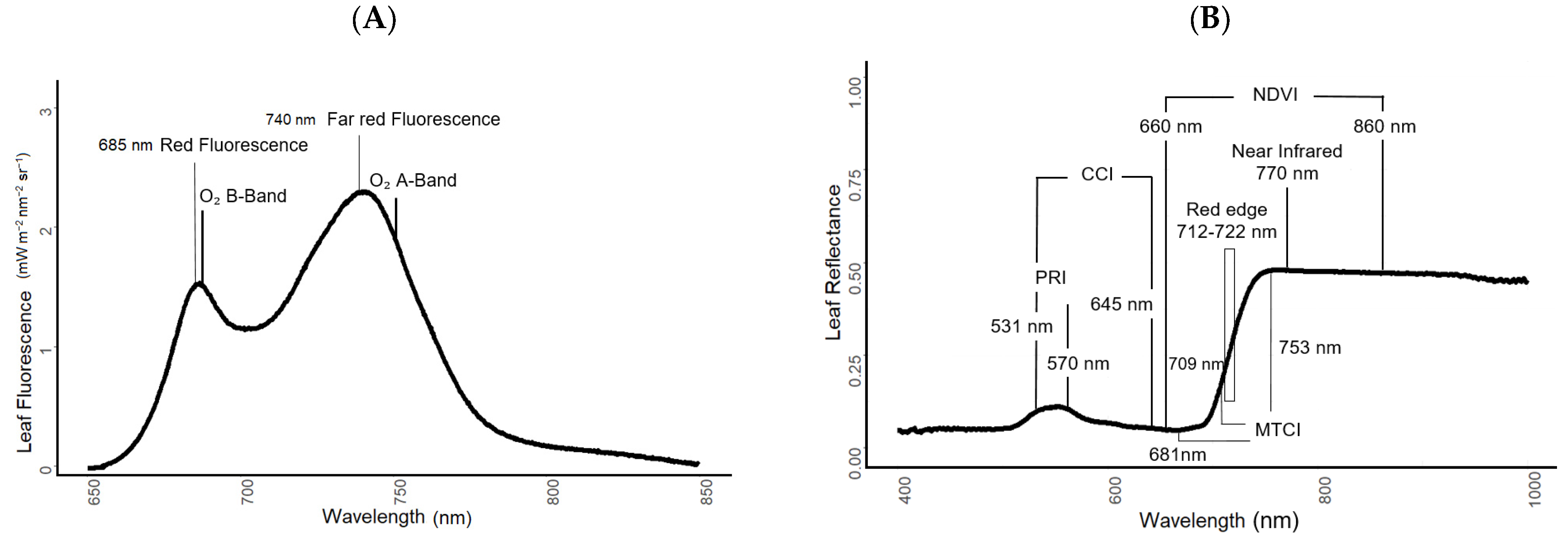
2.2.1. Fluorescence and Reflectance Measurements

The fluorescence and reflectance spectra of the leaves were measured under standardized conditions in the laboratory to facilitate intercomparability of results. These measurements were conducted using two separate spectrometers: a USB2000+ (Ocean Optics Inc., Orlando, FL, USA) for spectral fluorescence measurements and an ASD Hand-Held (ASD Inc., Boulder, CO, USA) for reflectance measurements with an integrating sphere. Note that canopy-level spectral measurements were conducted using two additional spectrometers coupled to a UAV (see below).
Spectral fluorescence measurements were conducted with a USB-2000+ spectrometer (range (R): 300–1100 nm, sampling interval (SI): 0.5 nm, full width at half maximum (FWHM): 1.5–1.8 nm). Attached to the spectrometer was a bifurcated reflectance probe (R600-7-VIS-125F, Ocean Optics Inc., Orlando, FL, USA) and fiber holder (RPH-1, Ocean Optics Inc., Orlando, FL, USA) used to conduct spectral measurements in the nadir position in order to maximize the fluorescence signal. The probe was connected to a filter carrier housing an OD4 short-pass 650 nm filter (Edmund Optics, Barrington, NJ, USA) to remove 99.99% of radiation above 650 nm and facilitate the measurement of spectral fluorescence. Finally, the filter carrier is connected to a halogen light source (HL-2000, Ocean Optics Inc., Orlando, FL, USA) through a fiber optic bundle.
Prior to spectral measurements, leaves were cut from shoots and dark acclimated for 20 min at room temperature. Spectral measurements were conducted at an integration time of 300 ms, and a dark current (DC) measurement was conducted prior to ChlF measurements and subtracted from the subsequent spectra. While this measurement technique allowed us to record the whole fluorescence spectra of the leaf, we only used the average of three measurements in the range from 685.110 nm to 685.780 nm and from 759.700 nm to 760.350 nm to represent F685 and F760, respectively (Figure 3A). For better comparability between leaf and canopy scale results, the 760 nm region was used for analysis instead of the 740 nm peak region. Further details on the measurement setup and protocol can be found in Rajewicz et al. [50].
Separately, a different subset of leaves was used to measure leaf directional-hemispherical reflectance spectra and estimate a range of reflectance indices (Table 3). Measurements were conducted using a RTS-3ZC Integrating Sphere (ASD Inc., Boulder, CO, USA) equipped with a halogen light (10 W, 6 V, Model 64225, Osram, Munich, Germany) coupled to an ASD Hand-Held Spectrometer (R: 325–1075 nm, SI: 1.6 nm, FWHM: 3.5 nm). Measurements were conducted at an integration time of 540 ms, and 10 spectra were averaged. A DC measurement was recorded before and after the measurements and subtracted from the spectra. Leaf directional-hemispherical reflectance factors were obtained by factoring the DC-corrected spectra obtained with the sample by those obtained using a Spectralon® panel (Labsphere, North Sutton, NH, USA) after Olascoaga et al. [51].

2.2.2. Specific Leaf Area

Specific Leaf Area (SLA) is calculated as projected leaf area (cm2) divided by leaf dry weight (g). Fresh leaf samples were scanned on white paper with a ruler for scale, allowing us to calculate the leaf area using the GNU image manipulation program (GIMP development team, 2021). The dry weight was measured after drying the leaves at 50 °C until no further weight decrease was observed.

2.3. Nutrient and Pigment Analysis

For nutrient analysis (all except N and C), samples were thawed and dried at 50 °C prior to analysis. Afterwards, the samples were homogenized, and 200–300 mg (dry weight) of each sample was taken for nutrient content analysis. Each sample was then mixed with 10 mL of HNO3 and 1 mL of H2O2. The samples were inserted into a MARS 5—microwave digestion system (CEM Corporation, Matthews, NC, USA), and digested for 10 min at 175 °C. After cooling, the resulting extract was filtered and analysed with the ICP-MS—mass spectrometer (Thermo Fisher Scientific, Waltham, MA, USA), using the method by Thomas [54]. The N and C concentrations of the leaves were analysed separately using a Variomax CN Analyzer (Elementar Analysensysteme, Hanau, Germany). To achieve dry weight, the thawed samples were dried for eight hours at 50 °C and homogenized with a mortar and pestle, after which 250 mg (dry weight) of each sample was analysed using the dry combustion method, where the samples are burned at 1000 °C in pure oxygen [55].
For leaf Cab and carotenoid pigment sampling, samples were thawed and 70 mg (fresh weight) of each sample was transferred into new tubes along with a pair of homogenization pellets and 1.8 mL of dimethyl sulfoxide (DMSO), after Wellburn [56]. Following a two-minute homogenization at 25 Hz, the samples were extracted for four hours in 50 °C. After extraction, the samples were centrifuged for 10 min at 3600 rpm (5810-R, Eppendorf, Hamburg, Germany) and the extracts analysed with a Shimadzu UV-1800 photometer (Shimadzu Corporation, Kyoto, Japan). Chlorophyll a and b and carotenoid values were estimated from absorbance measurements using equations by Wellburn [56] for DMSO:
Chlorophyll a = 12.47 × A665.1 − 3.62 × A649.1
Chlorophyll b = 25.06 × A649.1 − 6.5 × A665.1
Carotenoids = (1000 × A480.0 − 1.29 × Chl a − 53.78 × Chl b)/220
where A denotes the absorbance at a given wavelength in nm.

2.4. Canopy Measurements

2.4.1. SIF and Canopy Reflectance Measurements

For canopy reflectance and SIF measurements, we used a UAV-mounted dual field-of-view spectrometer system, a Piccolo Doppio [57,58,59]. This system houses two spectrometers: a QE Pro (Ocean Optics Inc., Orlando, FL, USA) (R: 639–805 nm, SI: 0.18 nm, FWHM: 0.31–0.35 nm) that was used for SIF measurements and a Flame spectrometer (Ocean Optics Inc., Orlando, FL, USA) (R: 344–1019 nm, SI: 0.39 nm, FWHM: 1.33 nm) that was used to measure canopy spectral reflectance. Irradiance and radiance were collected with a 25° field-of-view bifurcated fibre using a cosine-corrected fore optic.
While measuring, the UAV hovered for approximately 1 min above each measurement plot at around 8 m height, resulting in an approximately 1.77 m radius footprint on the plot. The flights were conducted on three separate days in 2018, July 10 (two flights), July 11 (three flights), and July 25 (four flights), between 09:30 and 13:00. The UAV also housed a nadir-looking GoPro—camera to be able to later control that the measurements were all done in appropriate positions. In addition to the measurement plots, a bare soil plot was also measured as a “zero plot” to provide validation for our SIF measurements. 25 spectra were averaged together and used to calculate plot-wise radiometric SIF and spectral reflectance factors as the ratio of upwelling radiance to downwelling irradiance using Matlab (The Mathworks Inc., Massachusetts). Integration times were algorithmically optimized, depending on the sky conditions. SIF was retrieved using the Spectral Fitting Method (SFM) [60] at spectral range 685.93–691.17 nm for oxygen B–band (hereinafter, and for better comparison with leaf level data, addressed as FY685 (C), where C stands for canopy) and 756.57–768.84 nm for oxygen A—band (hereinafter addressed as FY760 (C)). Further details about the flight plan and SIF retrieval methods can be found in Xu et al. [28].
For logistical reasons, it was not always possible to time the canopy spectral measurements with perfect clear sky conditions. Accordingly, some of the spectra data, especially during the early measurements, was collected under a variable cover of thin clouds (see Appendix D, Figure A14). In order to account for the potential impact of variable irradiance on the analysis of red and far-red SIF, we estimated and used the SIF yield instead, as follows:
F Y   685   C = F 685   C E P A R
F Y   760   C = F 760   C E P A R
where EPAR is the irradiance (W/m2, Appendix D, Figure A14) integrated for the PAR region between 400 and 700 nm.

2.4.2. Fractional Vegetation Cover Estimation

Fractional vegetation cover (FVC), defined as the projected vegetated percentage of the total study area [61], was here used to track the development of the potato crop canopy between early and late measurements as well as between treatments. FVC was estimated from multispectral images collected from two separate flights on July 10 and 25, 2018, with a MicaSense RedEdge M (AgEagle Sensor Systems Inc., Wichita, KS, USA) sensor. The flight height was approximately 54 m above ground level, providing a ground sample distance of 3.55 cm. The images were processed to orthomosaics with a GSD of 3.5 cm using Agisoft PhotoScan Professional commercial software (AgiSoft LLC, St. Petersburg, Russia). From the multispectral data collected by the camera on board the UAV, we chose to use the NIR band (centre wavelength 842 nm, bandwidth 57 nm) to classify each point in each plot into two categories, 0 s and 1 s, based on the reflectance of each pixel, using histogram-based segmentation with the QGIS-program (QGIS Geographic Information System. QGIS Association. http://www.qgis.org (accessed on 1 September 2022)). On each plot, the ground consisted of 0 pixels and the vegetation consisted of 1 pixels. This segmentation from histogram data allowed us to estimate the fractional vegetation cover for each plot as the ratio of the number of canopy pixels to the total (canopy + ground) pixels. More sophisticated approaches to estimating FVC are commonly applied, as NIR may be problematic under full canopy development [61]. However, due to the uncertainty of the data captured by the Micasense RedEge M—sensor in the visible wavelength in our study, we selected the NIR—band only.

2.5. Statistics and Linear Modelling Approach

To compare differences in leaf nutrient levels between the early and late measurements, we used the Wilcoxon signed rank test to determine whether the amount of nutrients had increased or decreased significantly. To detect differences between treatments within each measurement point, we used the Kruskal-Wallis one-way analysis of variance (ANOVA) to test for significance at p ≤ 0.05.
Multiple linear regression was used in the R-programming environment (R Core Team, 2021) to model leaf nutrient results as the dependent variables, using optical parameters as the independent variables. In the multiple linear regression model approach, a dichotomous “dummy” variable was added to the calculation to account for the subgroups of data, in this case the different measurement points. For each optical variable, the models for both individual measurement points were then checked for significance against the data from both measurement points with an ANOVA (p ≤ 0.05) test. In addition to the ANOVA-test, we plotted the pigments and nutrients against the spectral indices (Figures 8 and 9, Figure A1, Figure A2, Figure A3, Figure A4, Figure A5, Figure A6, Figure A7, Figure A8, Figure A9, Figure A10 and Figure A11 in Appendix B), and if the models were not significantly different, a red line was used to denote the linear model including both the early and late measurements, and the corresponding R2-value was added to the plot.

3. Results

The goal of our study was to characterize the relationship between greenness- and photoprotection-based vegetation indices, SIF, and the dynamics of foliar micro- and macronutrients using observations at the leaf and canopy scales. Changes in foliar nutrient contents, along with other leaf and canopy-level traits, were induced by four different fertilization treatments, two different water stress treatments, and their interaction with canopy development (Figure 2). We investigate the relationship between foliar nutrient contents and leaf spectral indices and how these relationships propagate to canopy level observations under the action of a dynamic canopy structure.

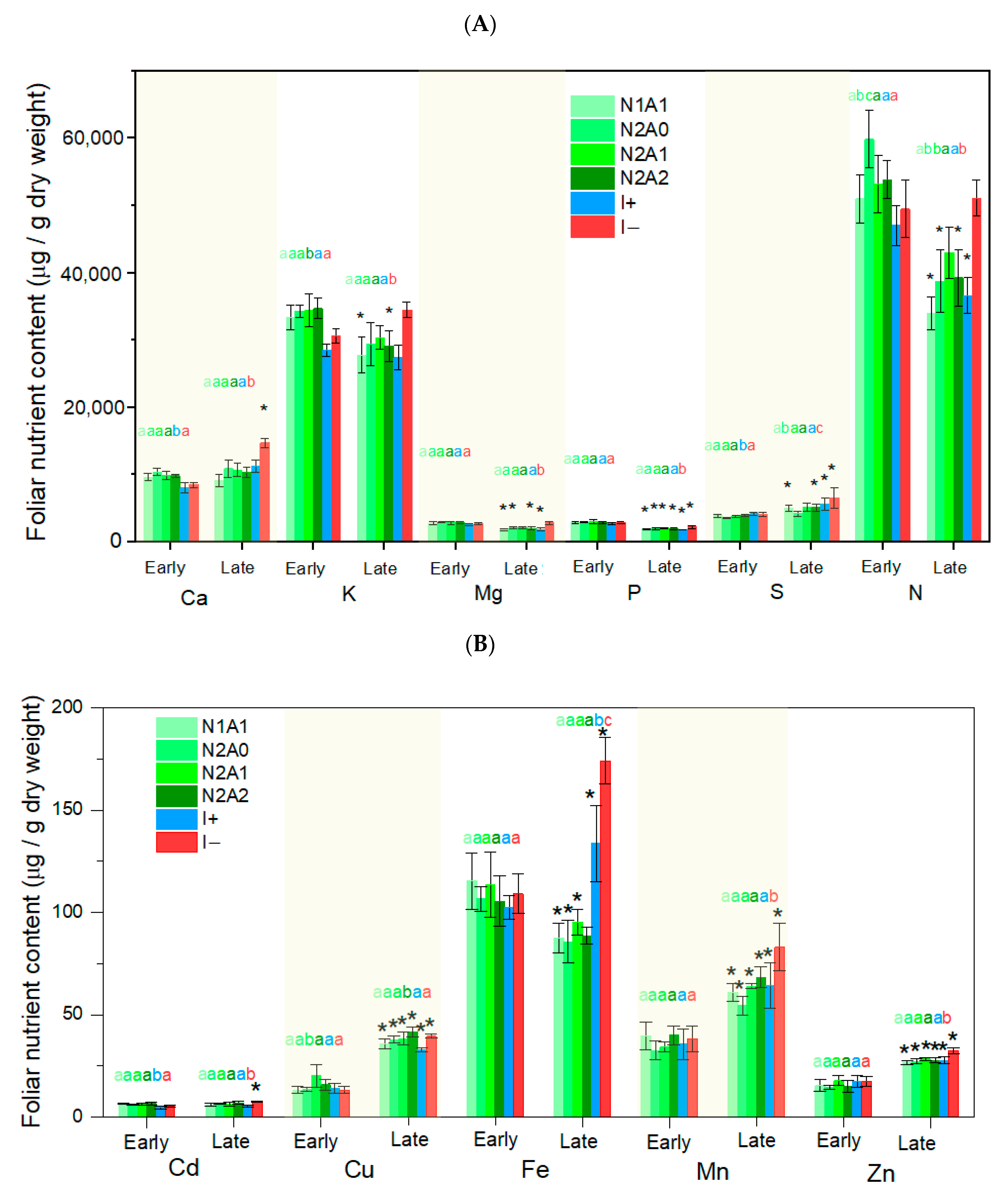
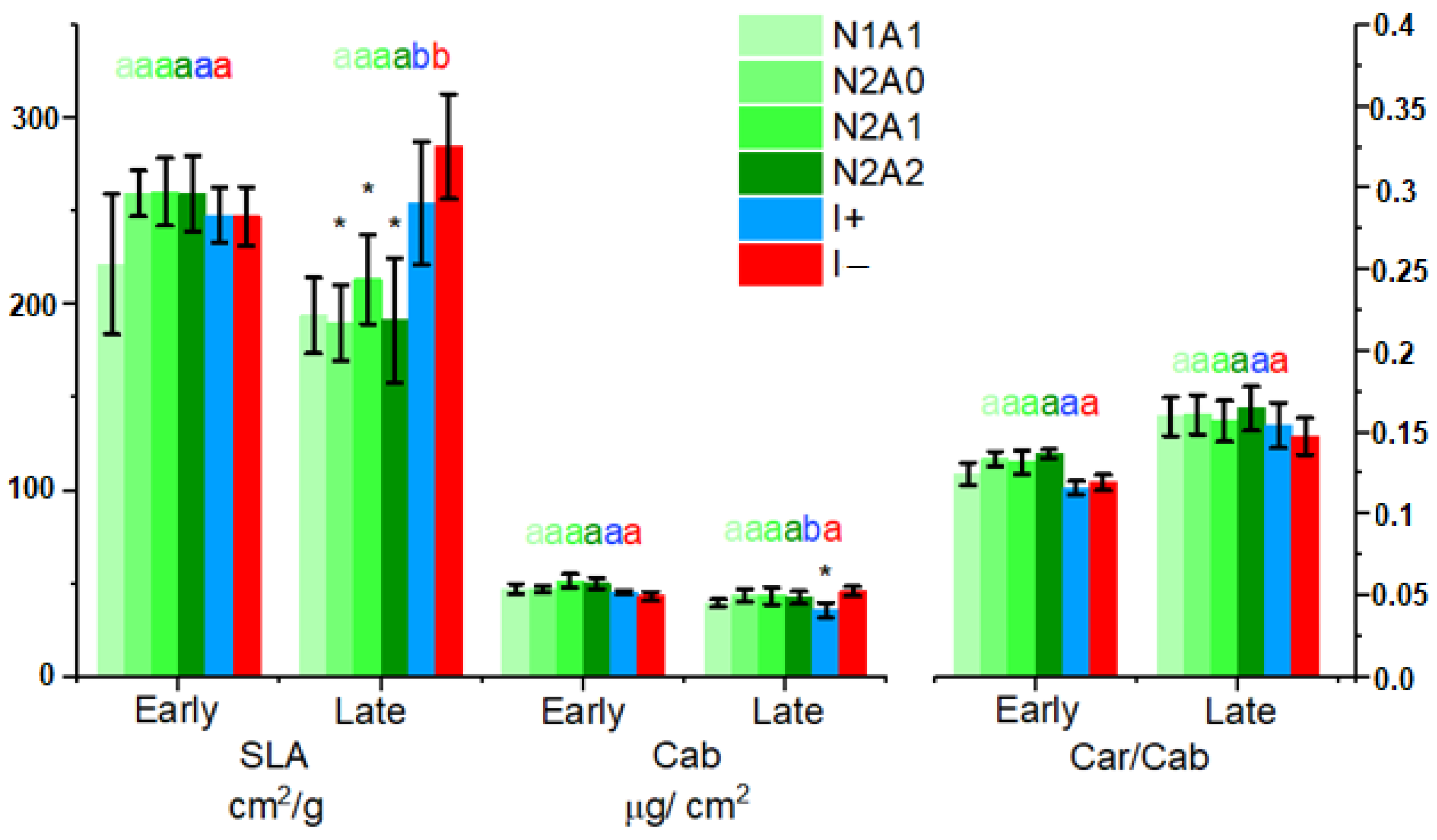
3.1. Leaf Level Nutrients

Variation in leaf-level nutrient contents were largely dominated by the variation between early and late measurements as canopy development interacted with nutrient and water stress treatments. Interestingly, foliar nutrient contents were not fully consistent with our applied range of fertilization treatments (Figure 4, Table 2), which could be related to the history of our experimental research site, which may have contained heterogeneous levels of background nutrients. However, significant differences in both foliar micro and macronutrient contents were observed both between treatments (small letters in Figure 4) and especially between early and late measurements (asterisk signs in Figure 4), allowing us to investigate their connection with the spectral indices.
Contrasting trends in the accumulation of foliar nutrients could be observed between the early and late measurements as the potato crop canopy was developing under the action of the nutrient and water stress treatments.
A group of nutrients (hereinafter Group 1), including the macronutrients K, Mg, P, and N, had a tendency to decrease across all treatments between early and late measurements (Figure 4A), whereas a second group of nutrients (hereinafter Group 2), including S, as well as the micronutrients Cu, Mn, and Zn, displayed a general tendency to increase with canopy development. The amounts of Fe decreased during the measurement period for the nutrient treatments, while in the water-stressed treatments, a strong accumulation could be noted. Finally, no temporal variation was registered in the foliar contents of Ca and cadmium (Cd), with the exception of the water stress treatment (I−) where all nutrient contents, excluding those of Group 1, significantly increased in concentration in response to the water stress treatment.
In terms of leaf morphological properties, no significant differences could be noticed in SLA between nutrient treatments during the early measurements (Figure 5) in response to our fertilization, and differences appeared only towards the late measurements, where SLA had significantly decreased in all treatments with full nitrogen load (N2A0, N2A1, and N2A2) denoting thicker leaves but remained unchanged or even increased in response to the water stress treatment (I−). Interestingly, despite the fact that the control water stress treatment (I+) was supplied with a full dose of fertilizer (N2A2), its SLA did not decrease between early and late measurements. These observations suggest a lower effectivity of the furrow irrigation when compared to the irrigation done by sprinklers. Furrow irrigation was used in the water-stressed control treatment (I+), which may have limited growth in the treatment.
In foliar pigment contents, we observed no significant differences in total chlorophyll a and b levels (Cab) between the nutrient treatments or between early and late measurements, with the exception of the control irrigation treatment (I+), where Cab levels had decreased relative to the first measuring point and the other treatments. Likewise, no significant differences could be observed in terms of carotenoid contents relative to chlorophyll (Car/Cab) between treatments or early and late measurements, although Car/Cab levels presented a non-significant increase as the canopy developed.

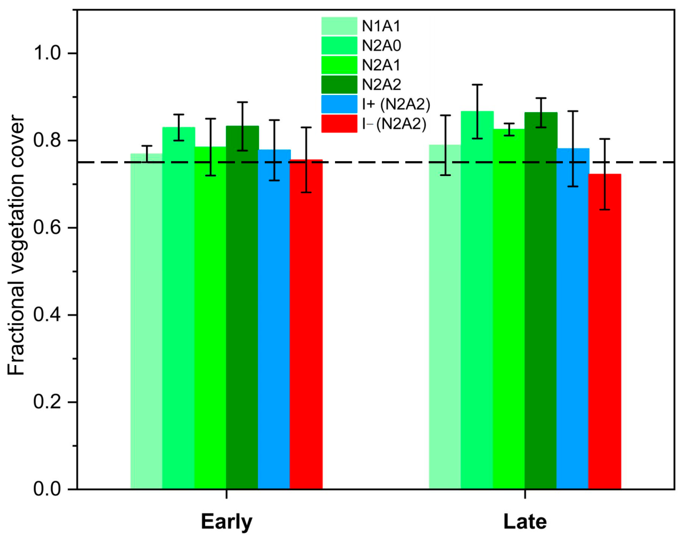
3.2. Fractional Vegetation Cover

We estimated FVC from multispectral canopy data to investigate how different treatments affected canopy development. We did not detect any statistical differences between the treatments or between early and late measurements (Figure 6). There was a slight tendency to increase in canopy fractional vegetation cover in the nutrient treatments with full N content, which could also be appreciated from our drone RGB imagery (Figure 1A) as a decrease in row gaps during the measurement period.

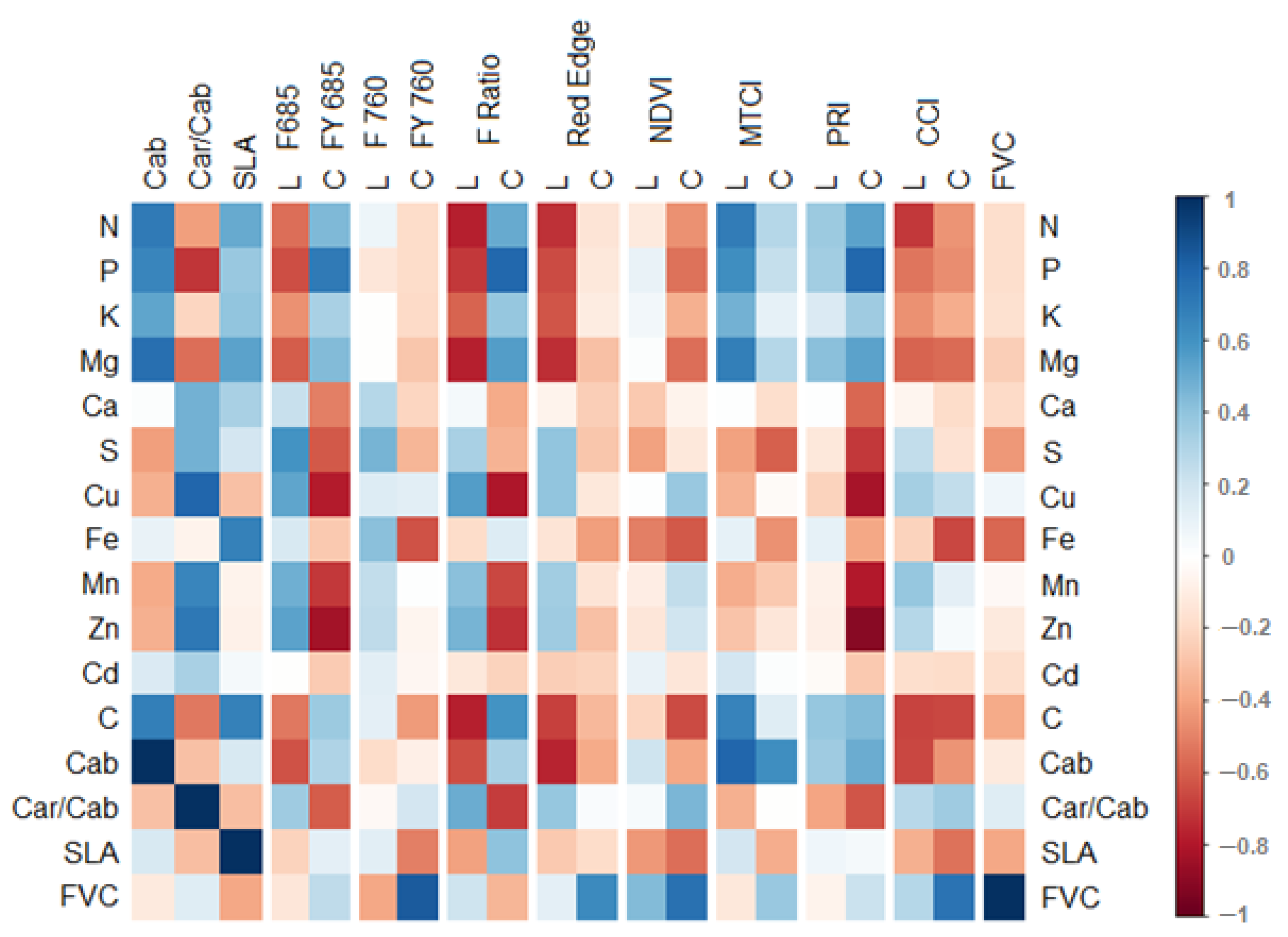
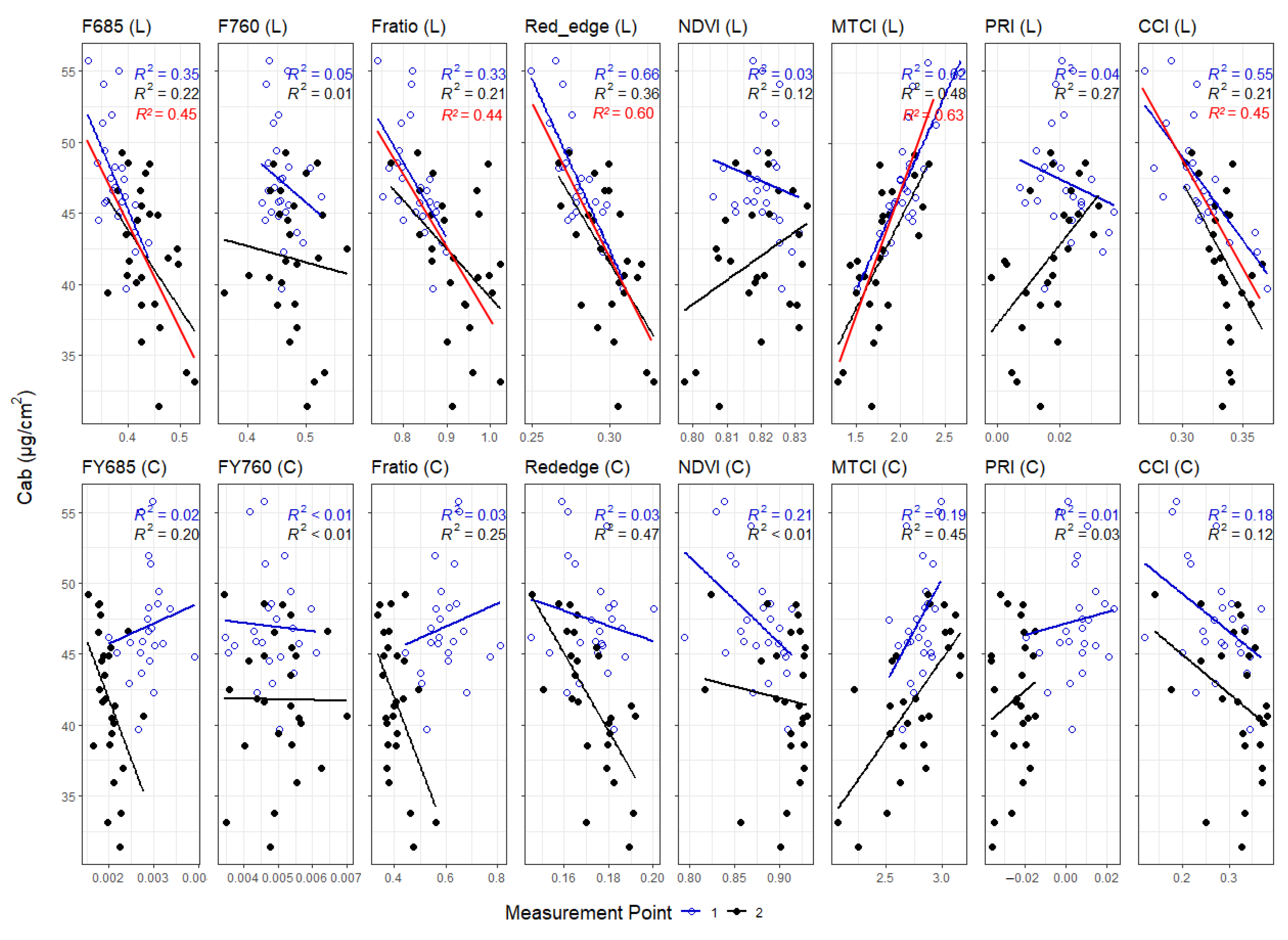
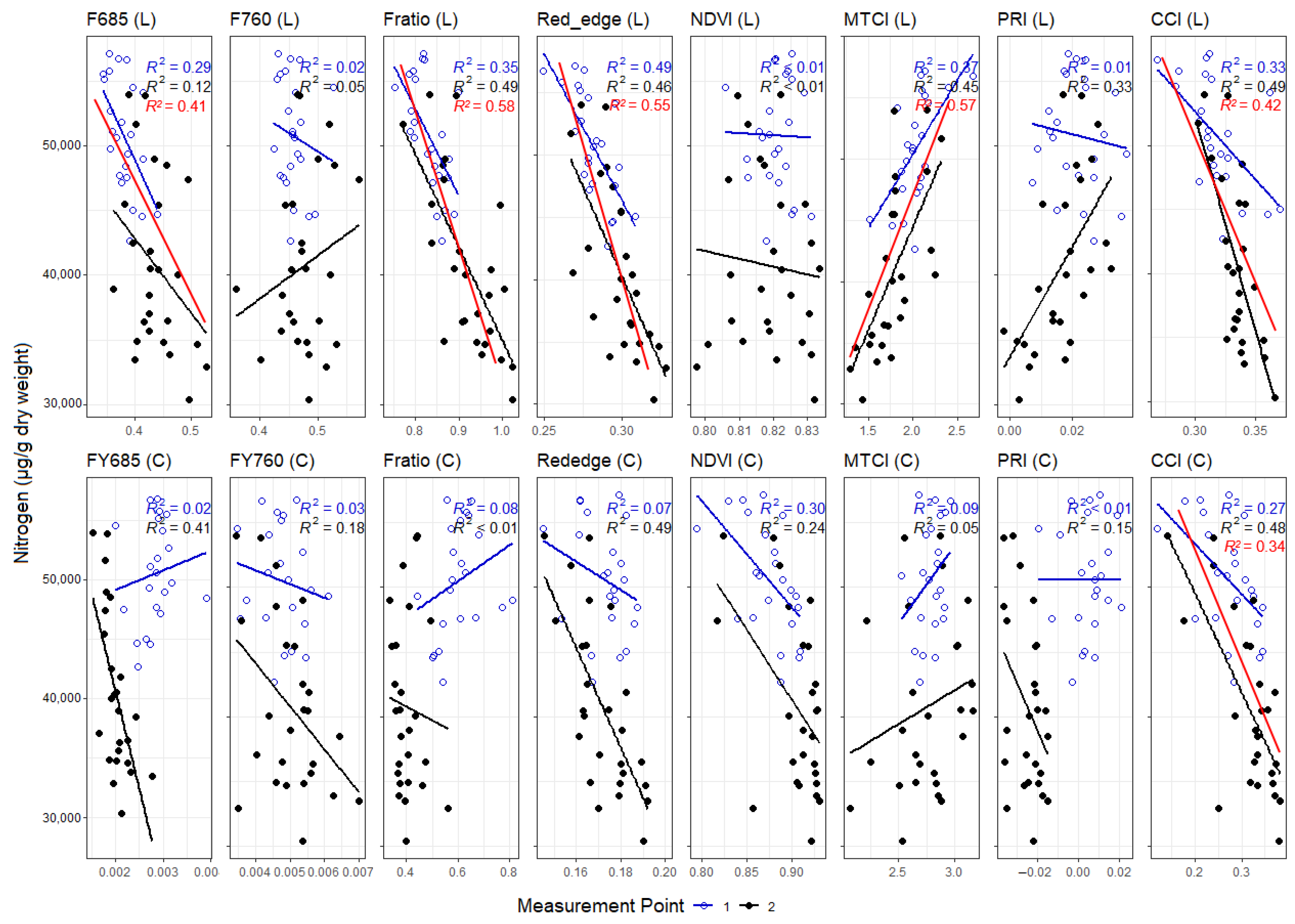
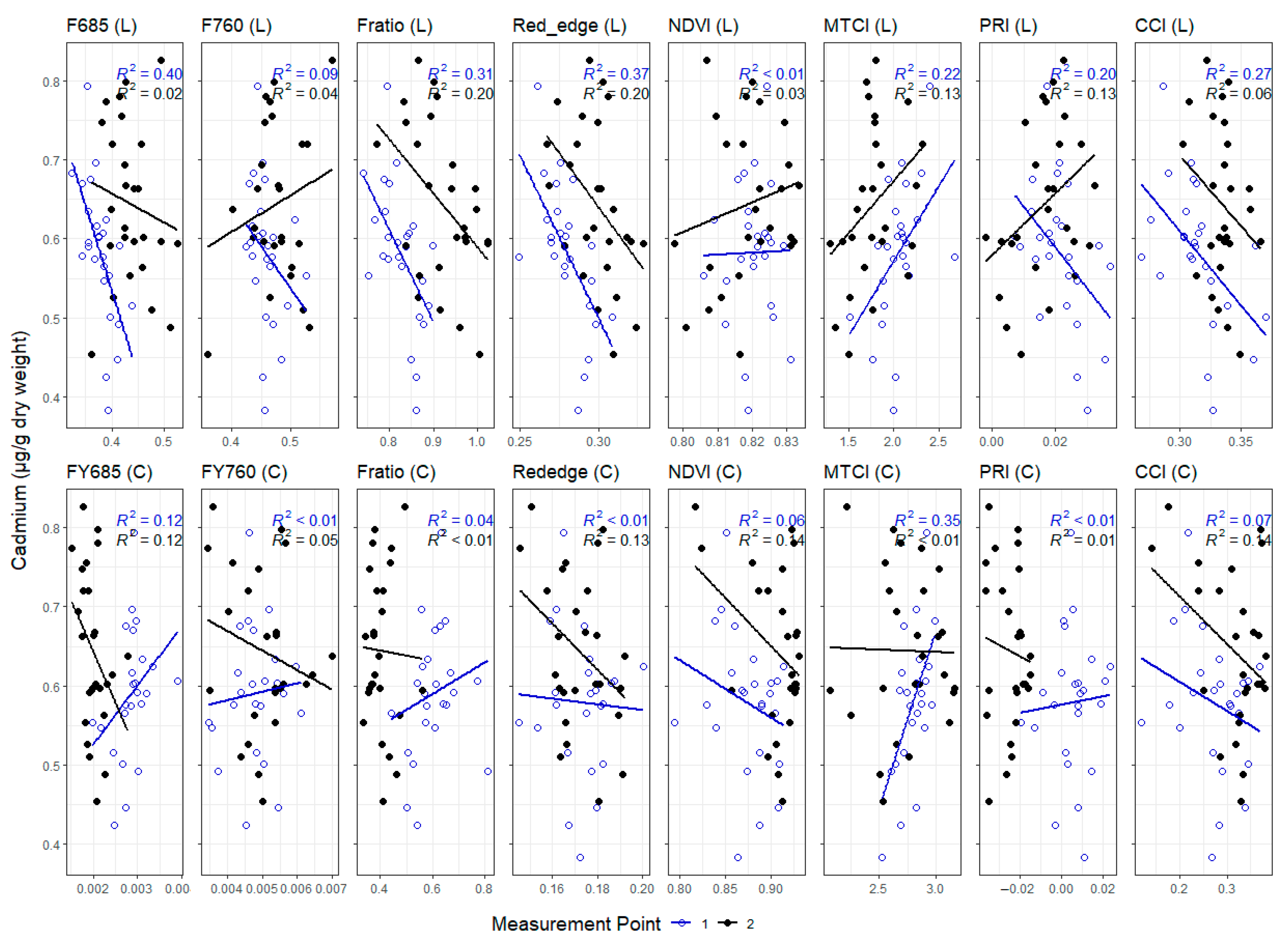
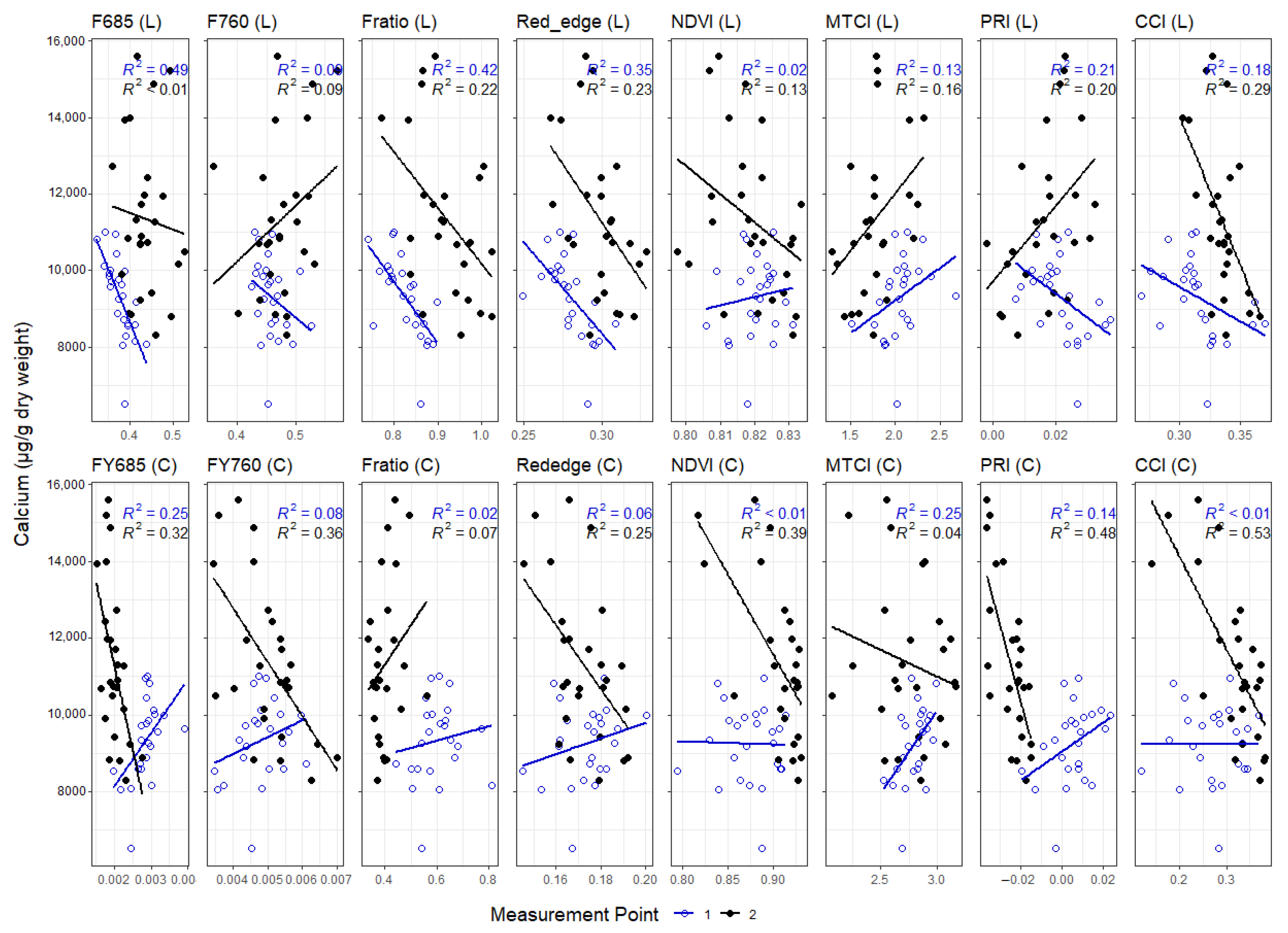
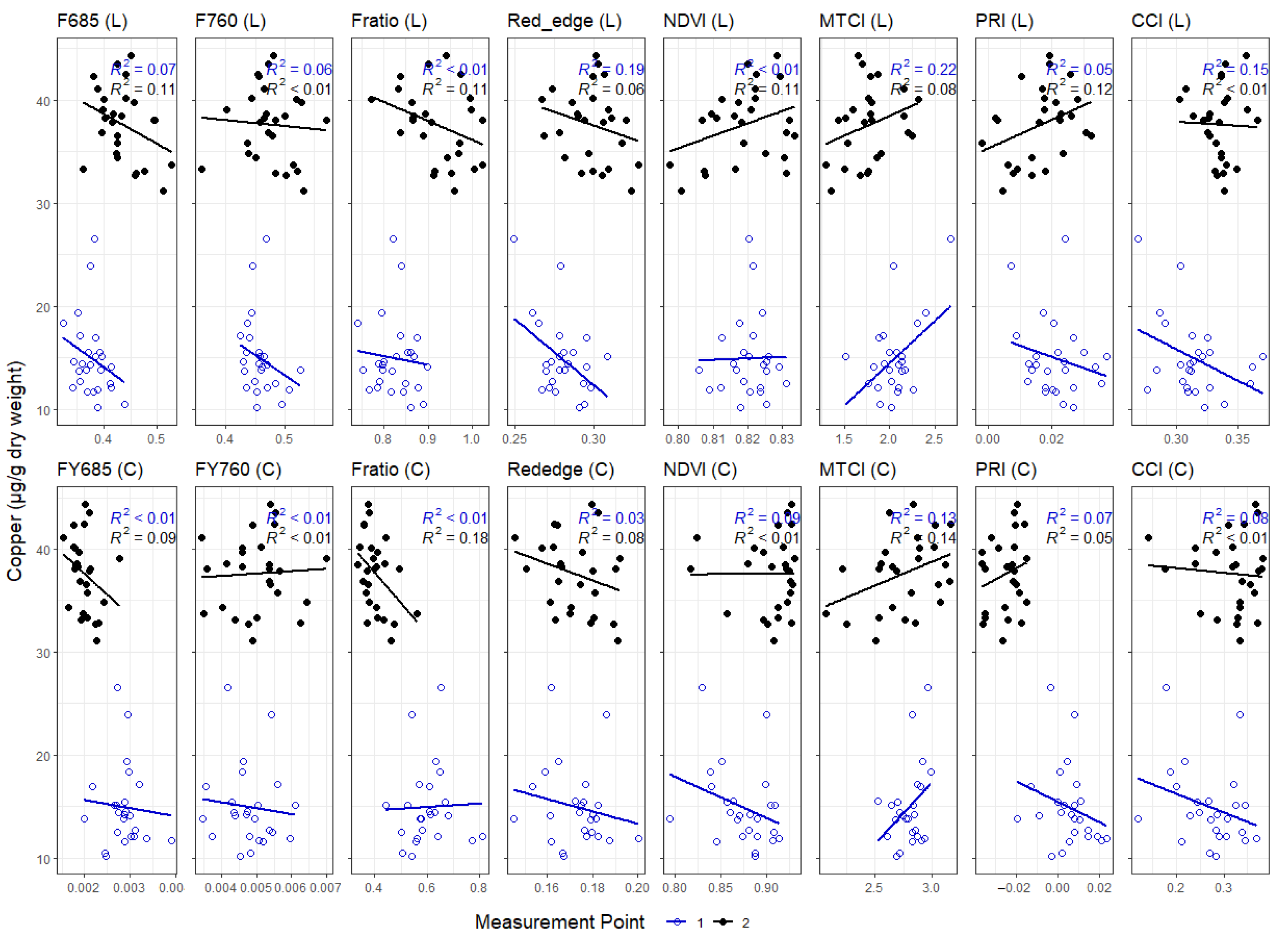
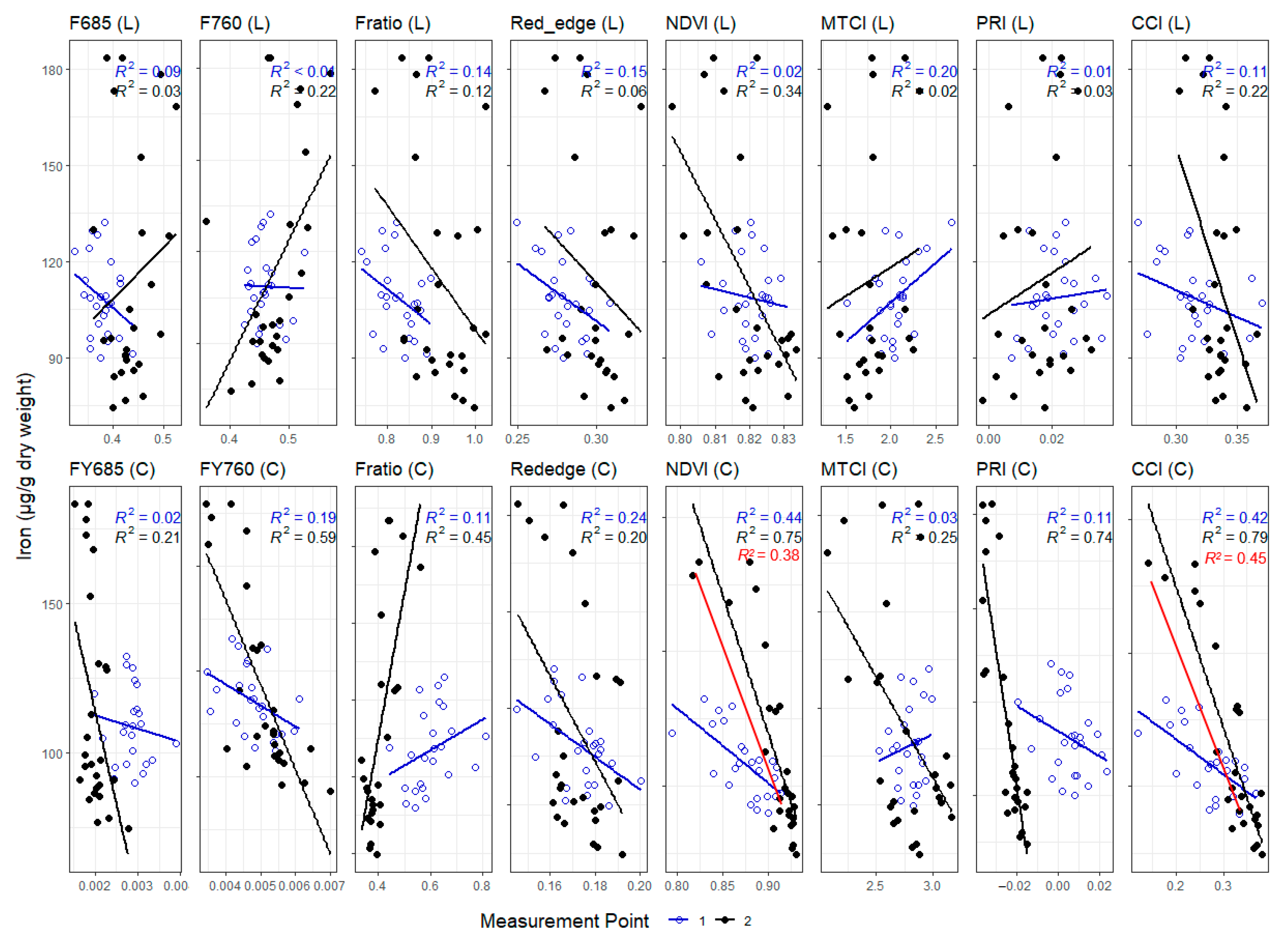
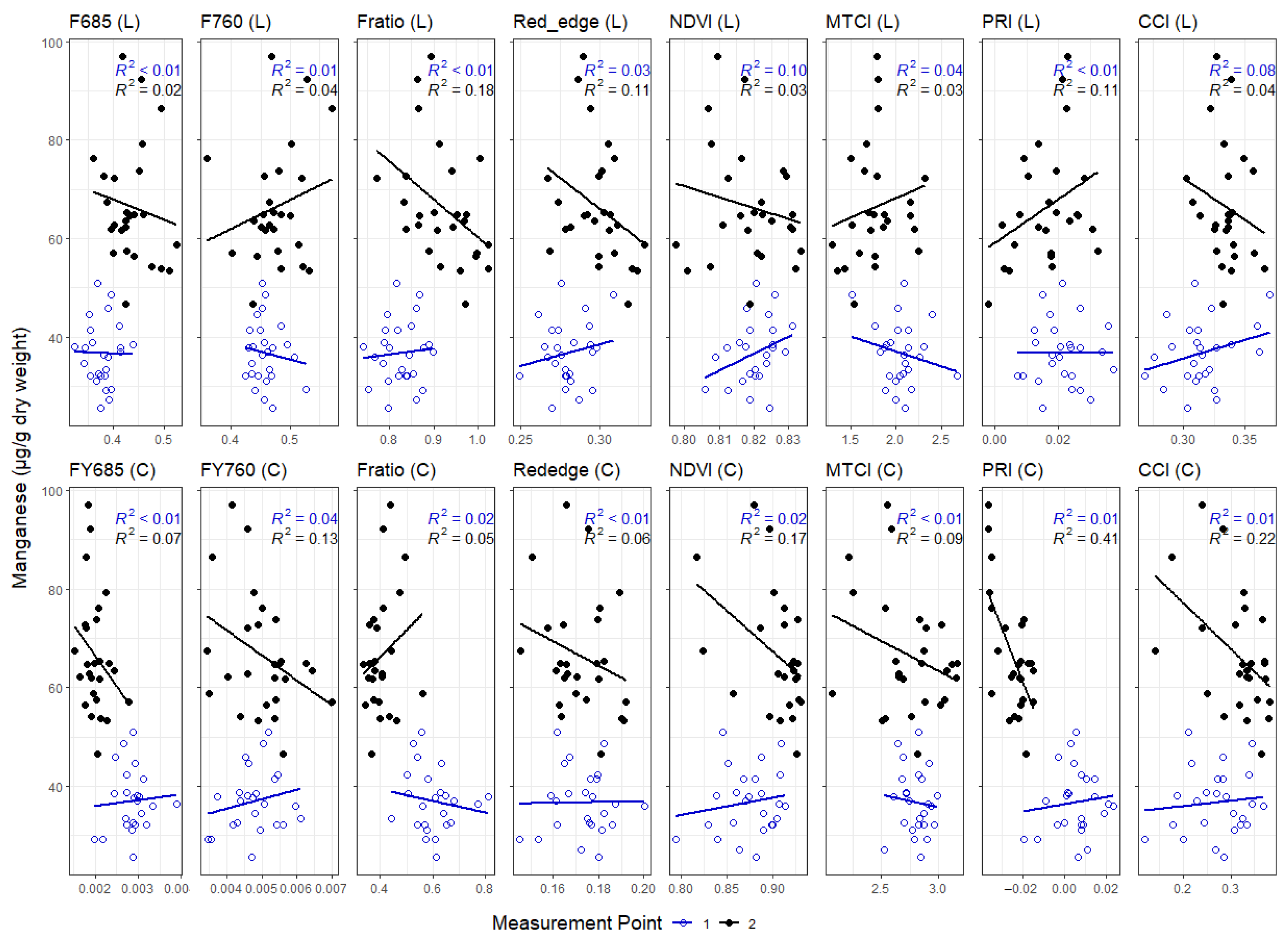
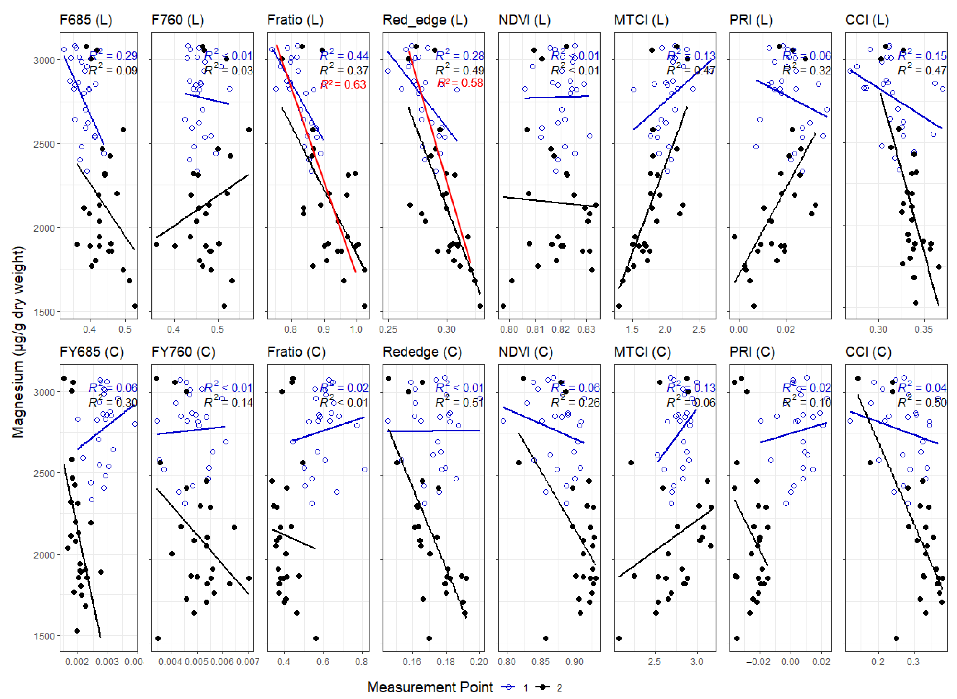
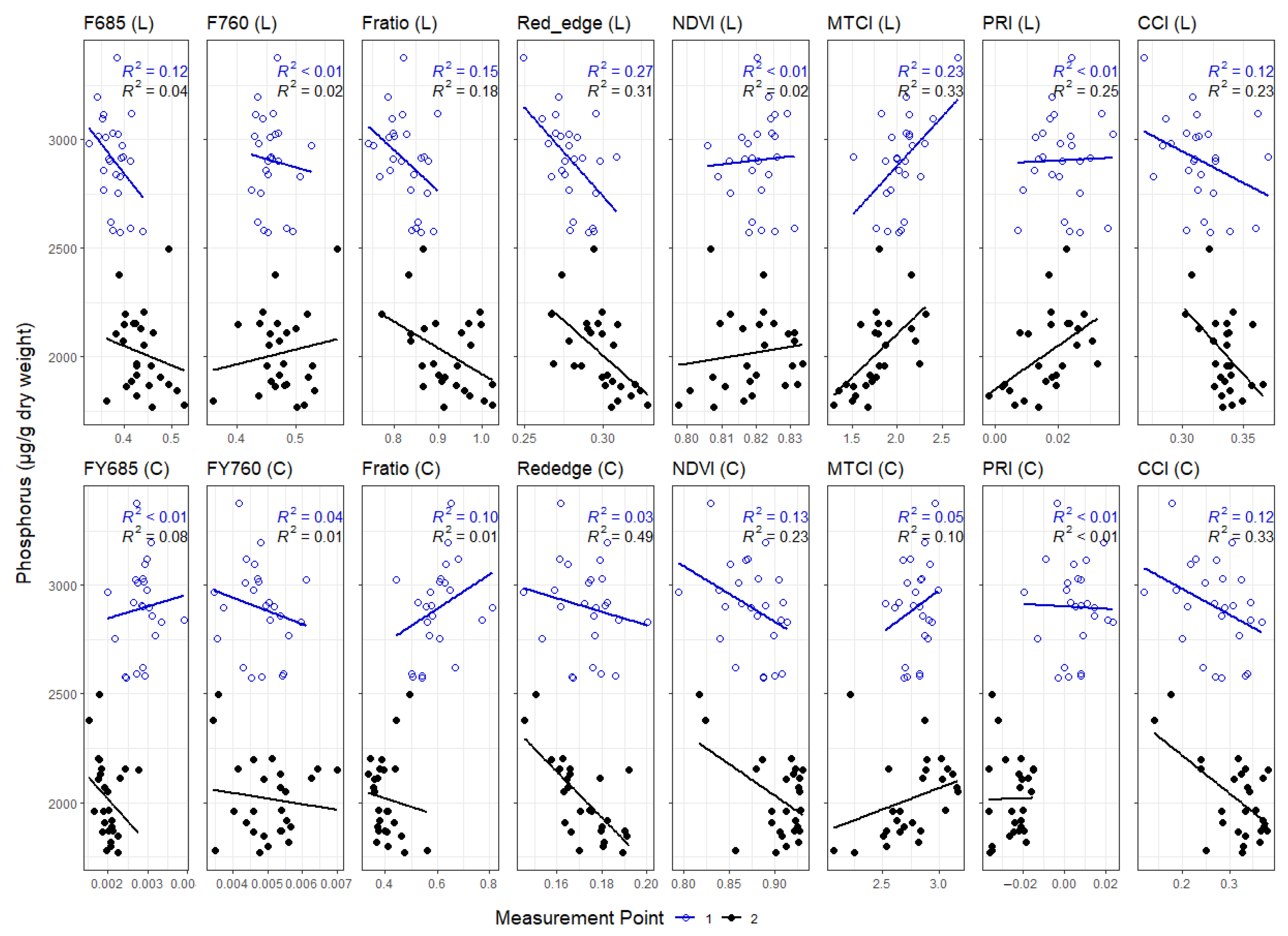
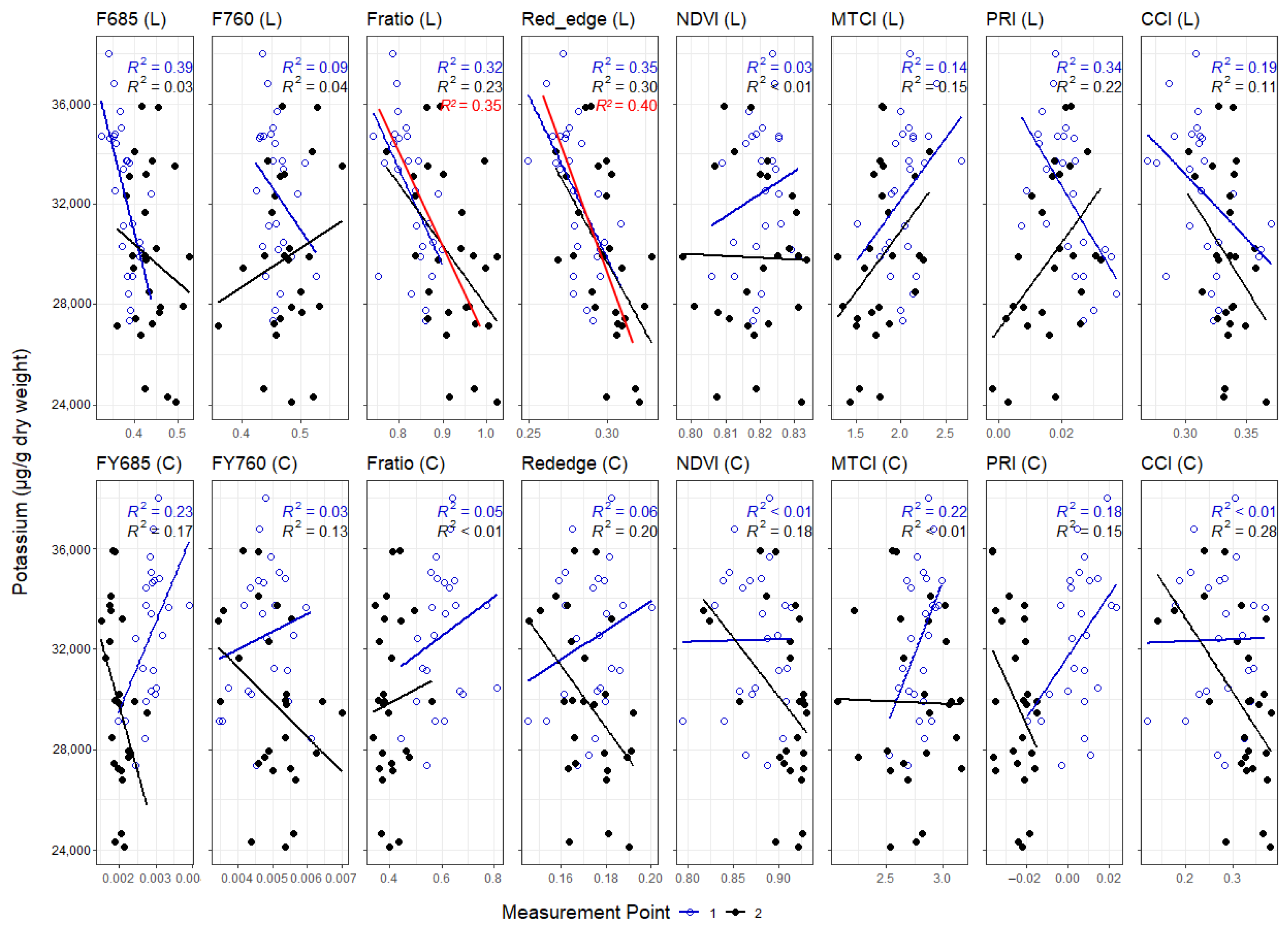
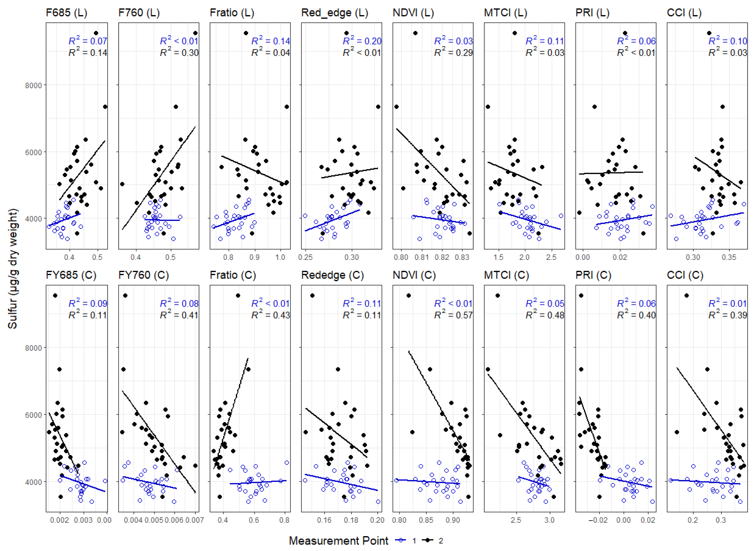
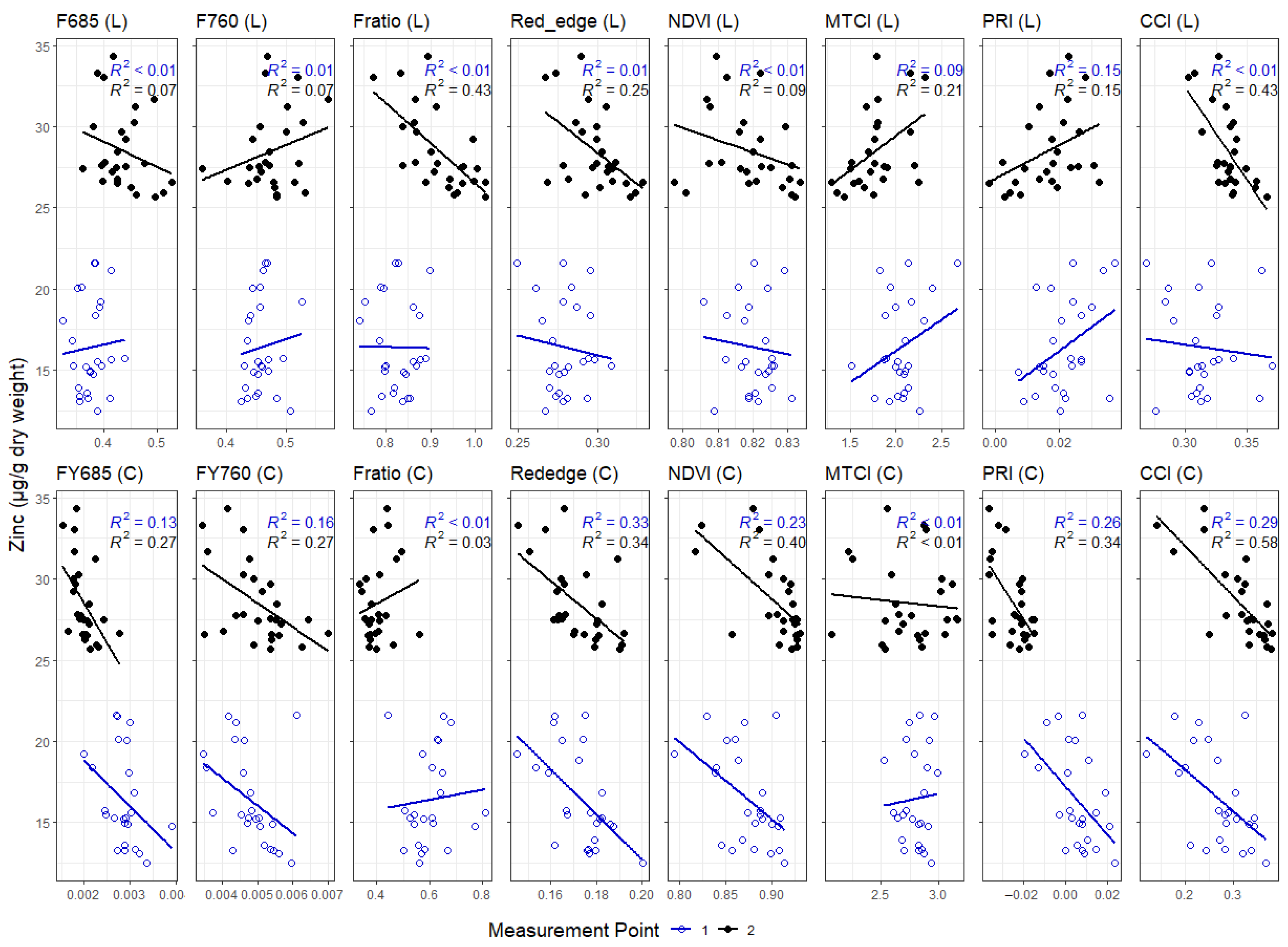
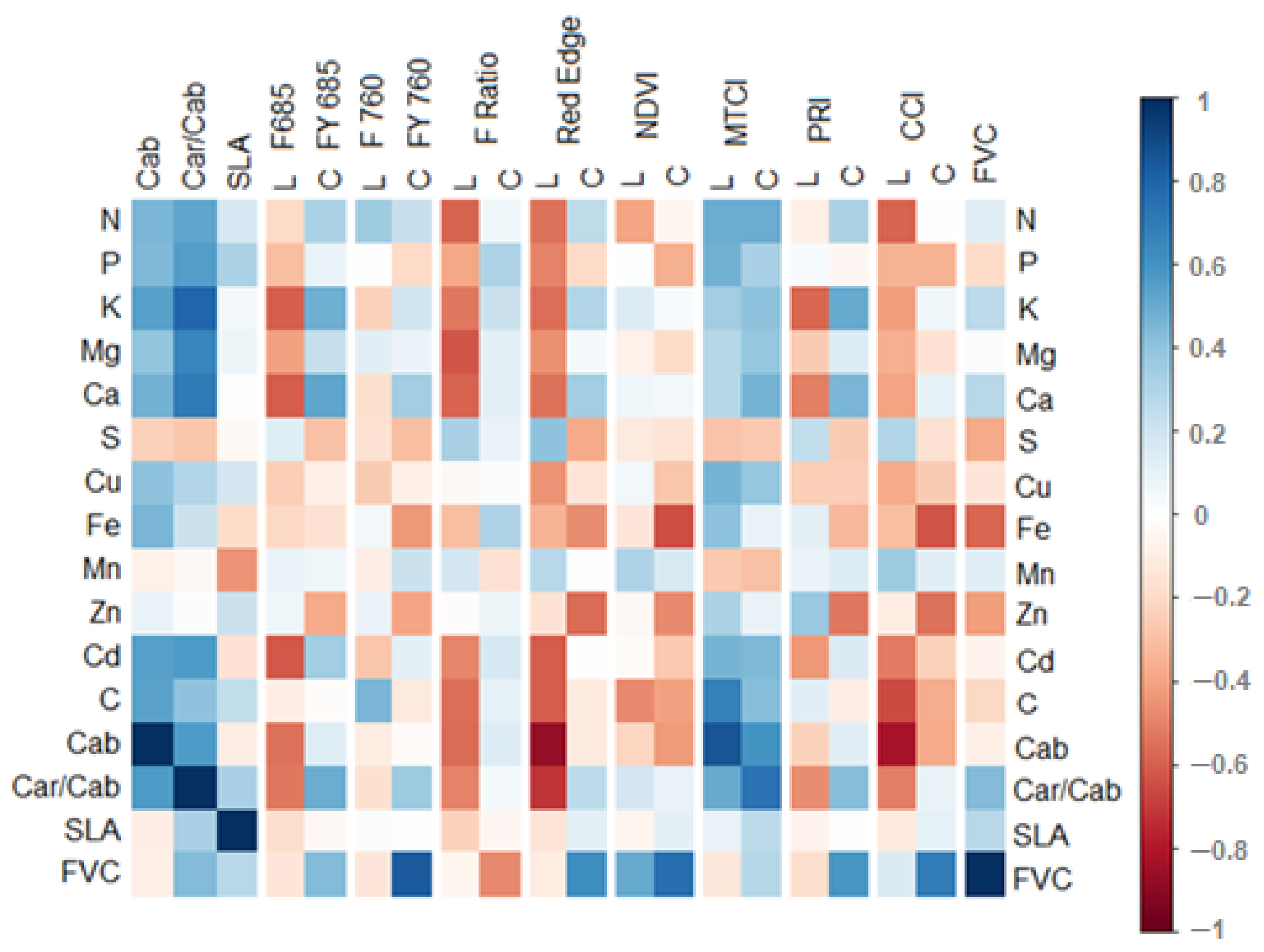
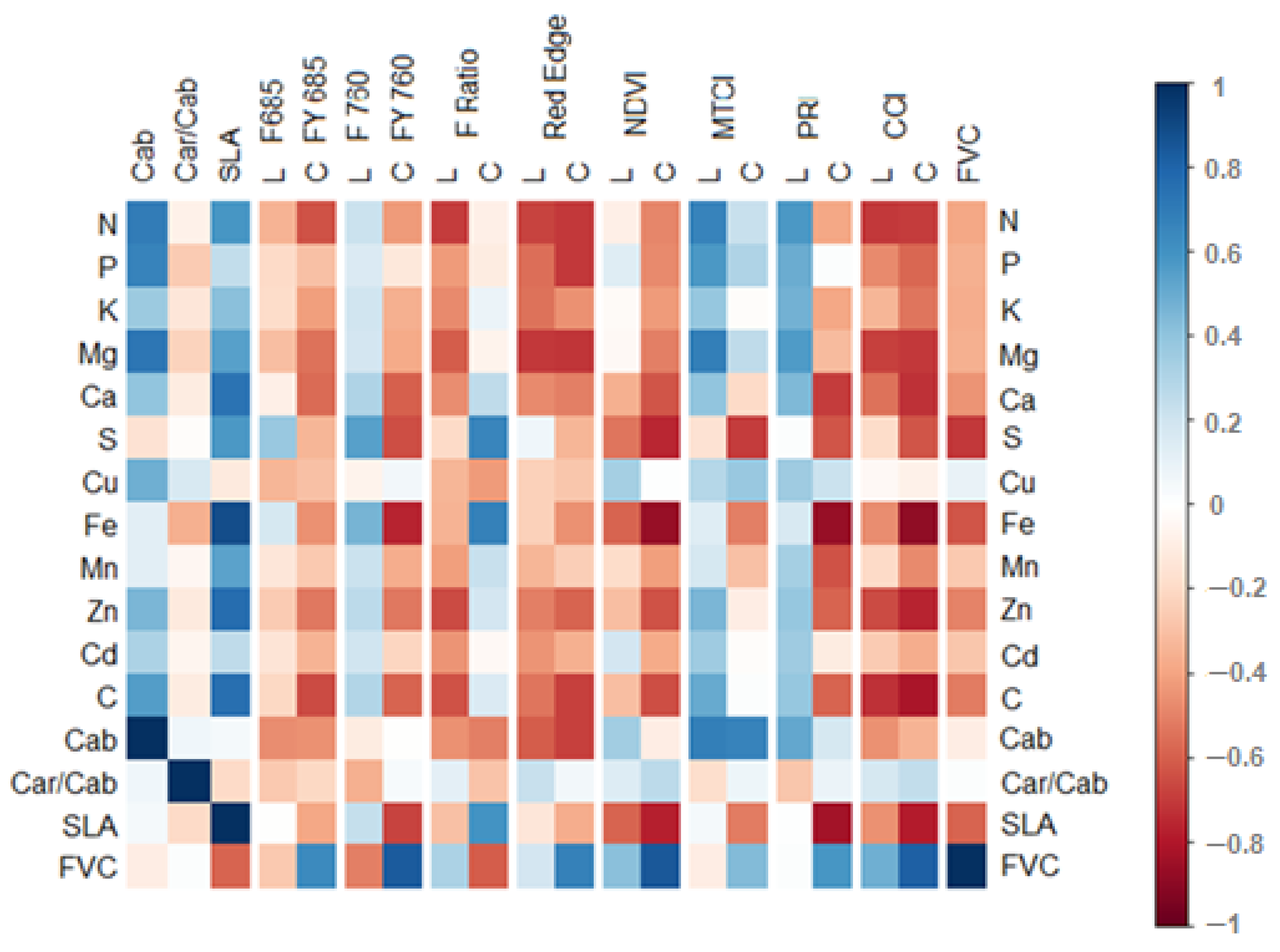
3.3. Correlations between Leaf and Canopy Spectral Indices and Foliar Nutrient Contents

Given that most of the observed variability in foliar nutrient contents took place over time between the early and late measurements (Figure 4A,B), we pooled together the results from both measurements in order to assess how the observed dynamics in foliar nutrient contents correlated with different spectral indices at the leaf level and how these relationships scaled up to the canopy level (Figure 7). In addition, correlations between different spectral indices and SLA, foliar pigment contents, and canopy FVC were used to investigate the factors underlying the correlations. A similar analysis was conducted separately for each of the measuring points (Figure A12 and Figure A13).
Correlations were clearly reflecting the grouping of nutrients introduced earlier, with Group 1 nutrients (macronutrients N, P, K, and Mg) being positively correlated to Cab and negatively correlated to Car/Cab, and Group 2 nutrients (including S and micronutrients Cu, Mn, and Zn) being negatively correlated to Cab and positively correlated to Car/Cab (see also Appendix E, Figure A15). When variability in foliar nutrient contents was reduced, such as in the case of Ca and Cd, or when examining the early and late measurements separately (Figure A12 and Figure A13), correlations with spectral measurements weakened or disappeared.
At the leaf level, the strongest correlations between VIs and nutrients were observed using the red-edge reflectance, which was negatively correlated with Group 1 macronutrients and Cab and positively correlated, albeit only slightly, with Group 2 nutrients. NDVI had only a weak negative correlation with Ca, Fe, and S, while MTCI was positively correlated with Group 1 nutrients and Cab and negatively but only slightly correlated with Group 2 nutrients. For fluorescence indices, F685 and the fluorescence peak ratio (F685/F760), Fratio, presented a similar pattern of correlation to those of red edge reflectance. In contrast, no correlations between nutrients and F760 were observed, other than minor positive correlations with Group 2 nutrients. For photoprotection-related indices, the CCI displayed again a similar pattern of correlation with Group 1, comparable to F685, Fratio, and red edge reflectance, whereas correlations with PRI were very weak and of inverted sign. In terms of carotenoids, the correlation between Car/Cab and PRI was slightly negative, as expected, but CCI was only negatively correlated to Car/Cab during the first measuring point (Appendix C, Figure A12). Overall, the strongest correlations between foliar nutrients and spectral indices were found for Group 1 macronutrients N, P, K and Mg.
At the canopy level, when pooling data over both early and late measurements, correlations between the red-edge and MTCI and foliar Group 1 macronutrient contents were drastically reduced compared to the leaf level, but a slight negative correlation between Group 1 nutrients and the NDVI appeared, which, at this scale, was positively correlated to FVC. In contrast, the canopy-level correlation between F685 or Fratio and foliar nutrient contents remained, but its sign inverted when moving from the leaf to the canopy scale. Interestingly, the correlation trends between FY760 (C) and foliar nutrient contents remained very weak, albeit with a reversed sign, despite the fact that FY760 (C) was positively and strongly correlated with FVC. In fact, the only nutrient that correlated with FY760 (C) was Fe, which turned out to be the nutrient with the strongest relationship to FVC (Figure 7). Similarly, strong correlations emerged also at the canopy level between foliar nutrient contents and PRI, here with positive correlations along with Group 1 nutrients and Cab and negative correlations with Group 2 nutrients and Car/Cab. For CCI, correlations with Group 1 macronutrients remained moderate and negative. Similarly, to FY760 (C), the strongest correlation was found between CCI and Fe. At this scale, CCI was also positively related to FVC and Car/Cab.
We also analyzed the correlations between spectral indices and leaf nutrients separately for each of the measuring dates (see Appendix B and Appendix C and examples in Figure 8 and Figure 9 for the cases of Cab and N, respectively). By separating the correlations between the early and late measurement we could visualize how the temporal development of leaf and canopy properties, in response to the nutrient and water stress treatments, influenced the relationship between spectral indices and leaf nutrient contents, allowing us to identify correlations that remained consistent over time as well as those that presented contrasting patterns, denoting changes in the mechanisms underlying the relationships.
In terms of Cab, the correlations in Figure 8 indicate that the relationship between leaf level F685, Fratio, MTCI, the red edge reflectance, and the CCI-index, and foliar Cab remained consistent over time despite potential variations in leaf thickness and morphology (Figure 5) between early and late measurements. Similar results were obtained for N in Figure 9. These results suggest that the leaf-level relationship between these spectral indices and Cab or N remains largely undisturbed by other factors. In fact, the relationship between Cab and N or Mg remained constant across early and late measurements, suggesting that the foliar partitioning of N and Mg into Cab synthesis would have remained constant (Figure A15). Yet, leaf-level correlations between spectral indices and foliar nutrients were not always consistent over time. For example, although the correlation between leaf level red edge and Ca (Appendix B, Figure A2) or between leaf level F685 and Mg (Appendix B, Figure A6) presented a similar slope, their intercepts were different, indicating that at least a third factor had changed between the early and late measurements affecting the relationship. Likewise, we also observed reversed correlation patterns between early and late measurements, such as in leaf level PRI and Cab (Figure 8) or leaf level F760 and K (Appendix B, Figure A8), suggesting that different factors mediate the relationships at different points in time. These patterns lead also to correlations that were of opposite sign within a single measuring point relative to the pooled dataset, such as for Fratio and Cu (Appendix B, Figure A3). Finally, we also identified situations where correlations were absent within a measuring day but appeared only when pooling data from the two measuring points, such as the relationship between F685 and Mn (Appendix B, Figure A5), suggesting that indirect interaction mediates the relationship between nutrients and spectral indices. For example, with nutrient contents influencing the leaf morphology instead of or above the stoichiometry of the photosynthetic apparatus.
At the canopy scale, we could also identify correlations that remained more consistent between early and late measurements, such as CCI and N (Figure 9), albeit many less than at the leaf level, which was expected due to the impact of a varying canopy structure not present in the leaf level correlations. For example, in the correlation between N, NDVI, and MTCI (Figure 9), the slopes remained similar between early and late measurements, but the intercept was different.
In addition, reversed correlation patterns could be found at the canopy scale, such as between Ca and Fratio (Appendix B, Figure A8). Similarly, as at the leaf level, these patterns lead to correlations that have an opposite sign within measuring points relative to the temporally pooled dataset; an example of this can be seen in the correlation between Zn and CCI (Appendix B, Figure A10) and Cu and CCI (Appendix B, Figure A3). Stronger correlations were found in the latter measurements between canopy optical properties and nutrients and pigments relative to the earlier measurements. For example, there were stronger correlations between Cab and canopy red edge reflectance, MTCI, and FY685 (C) in the later measurements, which were not evident in the earlier or pooled measurements (Appendix C, Figure A13), possibly due to the enhanced variability during the second measuring point once nutrient and especially water stress treatments had time to impact leaf and canopy development.
There were also some correlations between canopy spectral measurements and foliar nutrient and pigment contents that were weak within measuring point data, but emerged when pooling both early and late measurements together, such as, for example, between P and Fratio (Appendix B, Figure A7), emphasizing the influence of canopy development in mediating the relationships between foliar nutrient contents and spectral indices at this scale, which is discussed further in the next section.

4. Discussion

We investigated how the relationship between spectral indices and foliar macro- and micronutrient contents in potato plants was affected by canopy development under the action of different fertilization and water stress treatments, combining observations at the leaf and canopy scales. By doing so, we could compare the performance of different indices and elucidate possible mechanisms that underpin the relationships at the leaf and canopy levels (Figure 2). We measured foliar nutrient contents, pigments, SLA, and FVC as well as leaf and canopy spectral indices from four nutrient treatments and two water stress treatments at two different points in time, representing different states of canopy development and stress conditions. Our hypothesis was that through their more direct coupling to PAR absorption and photoprotection, ChlF and photoprotection-related indices would be more strongly correlated with foliar nutrient contents compared to vegetation indices related to plant greenness or chlorophyll content.
Results indicated that photoprotection-related indices such as the PRI and CCI, as well as F685 and the fluorescence Fratio, were more strongly correlated to foliar nutrient content dynamics compared to greenness-based indices when observed at the canopy scale and when observations across different stages of canopy development were pooled together (Figure 7). Furthermore, spectral indices, and in particular ChlF and photoprotection indices, had the potential to track variation across a wider range of foliar nutrients beyond the widely characterized N. These relationships were mediated by the dynamics in foliar pigment contents and leaf morphology (when observed at the leaf scale), as well as canopy structure (when observed at the canopy scale). In the following sections, we discuss the possible mechanisms underlying the observed relationships at the leaf and canopy scales, as well as possible steps towards future research.

4.1. Temporal Changes in Foliar Nutrient Contents Lead to Two Distinct Nutrient Groupings

Most of the observed variation in foliar nutrient contents during our study was caused by the temporal variation between our early and late measurements. We found that top canopy foliar contents of macronutrients N, P, K, and Mg tended to decrease over time in response to the combined effects of canopy development, fertilization, and water stress treatments (Figure 4). When considering all the data together, these macronutrients (Group 1) were positively correlated to foliar Cab (Figure 7 and Figure A15). In turn, the contents of micronutrients Cu, Mn, and Zn, as well as macronutrient S (Group 2), tended to increase over time (Figure 4) and were inversely related to Cab (Figure 7 and Figure A15). The patterns of variation in Group 1 and Group 2 nutrients, as well as their covariation with leaf level Cab and canopy level FVC, emphasized the observed relationship between spectral indices and foliar nutrient contents at the leaf and canopy scales, which we discuss in the following sections.
It is worthwhile noting the special increase in foliar nutrients observed in the water-stressed I− treatment, where in addition to Group 2 nutrients, Fe, Ca and Cd also accumulated in the top canopy leaves. These patterns could reflect the impact of the water stress in the I− plots, which, combined with the high temperatures during our experimental period (Figure 1B), would have interfered with overall canopy development, promoting the accumulation of nutrients in the new leaves at the top of the canopy. In fact, low canopy leaves in I− started to senesce a few days after our measurements, which would be compatible with a relocation of nutrients to top canopy (younger) foliage under drought stress [62]. The observed increase in SLA in I− (Figure 5) as well as the decreasing trend in FVC observed in the I− treatment compared to other treatments (Figure 6) suggest that canopy development in I− treatment was water-limited.
The contrasting temporal dynamics observed between the macronutrient-dominated (Group 1) and Group 2 nutrients could be partly explained by the increased biomass of the plants. This increase leads to a so-called dilution phenomenon [63] caused by an increasing demand for macronutrients in e.g., cell-wall formation, which decreases macronutrient concentrations in the leaves [64] and has also been noted in earlier research on potato plants for N, P, and K [63,65]. In micronutrients, there was a noticeable pattern of accumulation on the top leaves during the measurement period, with the exception of Fe. This could in part be caused by the relatively high background amount of micronutrients in our experimental fields [66].
The photosynthetic role of Group 1 nutrients K, Mg, N, and P is well documented across species [67,68,69], being essential constituents of proteins and chlorophyll (N, Mg), energy transfer and ATP synthesis (P), as well as stomatal movement and chloroplast structure (K). Notably, we found a highly consistent and positive relationship between N, Mg, and Cab throughout the study (Figure A15) indicating that the allocation of these nutrients into chlorophyll synthesis remained stable over time. Positive, albeit less consistent, correlations were also found between Cab, P, and K. It is therefore reasonable to state that Cab dynamics played a central role in mediating the leaf level correlations between spectral indices and Group 1 nutrients, either directly, as in N and Mg, or indirectly.
In terms of Group 2 nutrients, previous research by Pätsikkä et al. [70] showed that increasing leaf Cu in bean plants (Vicia faba L.) leads to a lowered Cab concentration in leaves. Additionally, it has been demonstrated that higher S levels in wheat have a negative effect on leaf Cab contents [71] and that Zn deficiency decreases leaf Cab amounts in pecan (Carya illinoensis) [72] by limiting C fixation and protein synthesis. Earlier research on tomato plants has also shown that too low or high concentrations of Mn in leaves decrease leaf Cab concentrations [73]. Overall, these studies support the negative correlations found here between Group 2 nutrients and Cab (Figure 7), which again would support the indirect role of Cab, in addition to leaf morphology, in mediating the correlation between Group 2 nutrients and our spectral indices.

4.2. Foliar Pigment Contents and Leaf Morphology Mediating the Leaf-Level Relationship between Nutrients and Spectral Indices

Nutrients from Group 1 were found to be negatively correlated with leaf level F685, Fratio, red edge reflectance, and CCI (Figure 7), while MTCI was positively correlated with the same macronutrients. Opposite patterns, albeit much weaker, were observed between these indices and Group 2 nutrients, which also presented weaker correlations with Cab. Likewise, nutrients that did not correlate with Cab, such as Ca, Fe, and Cd, presented the weakest correlations with spectral indices at the leaf level, further emphasizing the role of Cab in mediating these leaf-level correlations.
The NDVI was poorly related to foliar nutrient content dynamics, which is consistent with previously reported limitations of the NDVI to track foliar N contents due to signal saturation at moderately low foliar Cab contents [74,75]. Unlike the NDVI, the MTCI, which has been formulated to track Cab contents [52], was positively correlated with foliar Cab and therefore directly related to the nutrients from Group 1 (Figure 7). In turn, the negative correlation between Cab and red edge reflectance is consistent with the effect of increased Cab amounts shifting the red edge feature towards higher wavelengths [76], thus decreasing the reflectance in the measured red edge region (Table 3), making it less susceptible to Cab saturation compared to the red reflectance bands [77]. Leaf-level reflectance indices using the red edge reflectance region have been previously shown to correlate well with foliar N [78] and Cab [76] amounts in potato plants or with foliar Cab and Mg contents in different wheat genotypes [79], which is in line with our results that expand these observations to other macro and micronutrients.
In turn, the negative correlation between leaf-level F685 and Fratio, and nutrients from Group 1 and Cab (and the opposite for Group 2 nutrients) (Figure 7) could be explained in terms of the re-absorption of red fluorescence photons by chlorophyll inside the leaf [36]. Specifically, at low Cab contents, where reabsorption is minimal, a marginal increase in Cab leads to an increase in PAR absorption and therefore an increase in fluorescence across all wavelengths (F685 and F760). In contrast, at higher Cab contents, like the ones observed in our leaves (Figure 5), a marginal increase in Cab has a very small effect on PAR absorption due to self-shading inside the leaf but can further increase the reabsorption of fluorescence in the red fluorescence bands that overlap with the chlorophyll absorption spectrum [28,36,37]. This phenomenon would explain the poor correlation between F760 and Cab (and, by extension, nutrients) observed in our study (Figure 7), as well as the negative correlation between F685 or the Fratio and Cab and their subsequent relationship with the nutrient groups.
Wang et al. [25] recently reported how steady state PAM fluorescence (Ft), integrated from 697–750 nm as measured with a FluorPen FP110 (PSI, Brno, Czech Republic), was strongly correlated to foliar N contents. This contrasting observation could be due to the lower foliar Cab contents in their almond experiment relative to our potato leaves, where far-red fluorescence would be less saturated, or to the different spectral coverage between studies. Foliar N has also been known to be detectable by red fluorescence and the red to far-red ratio, for example, in wheat [43] and turf grasses [80]. However, as Ač et al. [81] point out, the relationship between fluorescence and foliar N can be either positive or negative, changing with how re-absorption and various leaf level processes affect it, which may be an important consideration when observations are conducted in developing or senescing leaves. Here, we extend these results showing that not only N but also macronutrients P, K, Mg and S, and micronutrients Cu, Mn and Zn coexist with F685 as well as Fratio.
In terms of photoprotective pigment related indices, the CCI-index was found to be negatively correlated with nutrients from Group 1 as well as foliar Cab (Figure 7), while PRI was positively correlated with the same nutrients and Cab, albeit weakly. As expected, PRI was negatively correlated with Car/Cab (Figure 7), while CCI had a weak positive correlation with it. At the leaf level, both CCI and PRI are expected to be inversely related to photoprotection via their sensitivity to the carotenoid/chlorophyll ratio [30,82]. In other words, when leaves present increased levels of photoprotective carotenoid pigments relative to chlorophyll, the PRI and CCI values should decrease. The difference between these two indices is that CCI uses 645 nm as a reference band, which is near the peak Cab absorption wavelengths and is thus expected to more accurately reflect changes in Cab amounts relative to the PRI, which uses the 570 nm band as reference instead [30].
Gitelson et al. [83] found a strong relationship between PRI and Car/Cab in maize and soybean (Glycine max) and noted that in a period of water limitation where Cab decreases, PRI did not follow foliar Cab contents. Our results would indicate that, unlike PRI, CCI was mostly driven by changes in Cab levels rather than Car or Car/Cab. When comparing our results to previous work, positive relationships between PRI and foliar Cab and N contents have been observed on top leaves of a variety of annual, deciduous and evergreen perennial species [47] and on Engelmann spruce (Picea engelmannii Parry ex Engelm.) with different N fertilization regimes [46]. Our results here are aligned with these observations, suggesting that the connection between carotenoid-based indices and foliar nutrient contents, via foliar pigment dynamics, can be expanded to other macro- and micronutrients.
It is important to note that when pooling all our results together as in Figure 7, although the mechanisms discussed in this section provide a direct (i.e., first order) explanation to the relationships between foliar nutrients, pigments and spectral indices, this does not imply that this is the only mechanism by which spectral indices are connected to foliar nutrient contents. As shown in our Appendix B, Appendix C and Appendix E, other factors, possibly related to indirect effects of our nutrient and water stress treatments or the development and morphology of leaves, also influenced the relationships and should be kept in mind when developing quantitative methods for data interpretation.

4.3. Impact of Canopy Structure on the Capacity of Spectral Indices to Track Foliar Nutrient Contents

At the canopy scale we also found evidence of a dichotomous split in correlations between optical indices and foliar nutrient contents (Figure 7). The nutrient groupings (Group 1/Group 2) remained consistent with the leaf level correlations, but the correlations displayed either an inverted pattern (FY685 (C) and Fratio), had strongly decreased (Red edge and MTCI), increased (NDVI but especially PRI) or remained similar (CCI). Clearly, these contrasting patterns were influenced by the dynamics in canopy structure that took place between measuring points in response to the fertilization and water stress treatments. It is important to note that we are here comparing canopy-level spectral data to leaf level nutrients, instead of canopy level nutrients. Canopy-level spectral data is often compared to scaled canopy nutrient contents using LAI or total leaf area [44,84,85]. Unfortunately, the indirect estimation of total LAI in our potato crop was highly challenging due to highly dynamic variation in leaf angle found in the same experiment [28]. In turn, direct estimation of LAI using destructive methods was not practical in the context of this experiment. Accordingly, we here focus our analysis on the correlations with leaf foliar contents, which remains a key parameter for crop modelling and management [25], avoiding adding an additional source of uncertainty. The implications of this point on the correlations between variables are discussed below.
In contrast to the leaf level results, greenness-based indices were largely uncorrelated with Group 1 nutrients, although a weak negative relationship appeared between Group 1 and NDVI. It is important to note however that all these indices, especially the NDVI, were positively related to FVC, suggesting that their correlation with nutrients would have probably improved if they would have been scaled to total canopy nutrient contents using LAI or total leaf area. In previous research, Nigon et al. [86] showed that MTCI was able to capture differences in leaf N concentrations, however, as reported earlier by Li et al. [18], vegetation indices based on the red edge region are susceptible to the impact of bare soil to the signal. This could in our case affect the signal and explain why the high correlation between N concentrations seen at the leaf scale can no longer be detected at the canopy scale.
The lack of a stronger correlation between NDVI and N at the canopy scale could possibly be due to the NDVI signal saturating even in moderate LAI conditions. In fact, the negative relationship between NDVI, Group 1 nutrients and Cab observed at this scale (Figure 7) would point to a causal relationship caused by the contrasting patterns observed here between Group 1 and Cab (tendency to decrease over time), and canopy development (tendency to increase over time). When correlations are analyzed separately within each sampling point, where variation in canopy structure remains smaller, the positive correlation between MTCI and Group 1 nutrients (Figure A12) or the negative correlation between red edge reflectance and foliar Cab and Group 1 nutrients (Figure A13) is maintained, as noted also in a previous study for N [87].
Overall, since canopy greenness indices are affected by FVC, their capacity to track foliar nutrient contents seems to be dependent on the covariation between FVC and foliar Cab, which was here very limited. In addition, soil reflectance effects may have also influenced our results as canopy closure tended to increase over the experimental site. The weaker correlations between greenness indices and foliar nutrients during the first measuring day (Figure A12), when FVC tended to be lower, could support such an effect. Likewise, variability in incoming illumination during the first measuring point could have also contributed with some uncertainty (Figure A14).
In terms of ChlF, canopy FY685 (C) and Fratio presented inverted patterns of correlation with foliar nutrients relative to leaf scale measurements, whereas canopy FY760 (C) remained largely uncorrelated to foliar nutrient contents. The strong relationship between FY760 (C) and FVC across the dataset (Figure 7, Figure A12 and Figure A13) points to the importance of canopy structure and cover fraction in determining chlorophyll fluorescence variation at the canopy scale.
As with leaf scale, canopy ChlF is also driven by APAR (modulating both FY685 (C) and FY760 (C)) and reabsorption (influencing FY685 (C)). However, in contrast to the leaf level, where these mechanisms are mediated by foliar Cab amounts, at the canopy scale they are additionally mediated by the amount, arrangement, and dynamics of leaves and their angles [28,37,88], here pooled together into a fractional vegetation cover (FVC) parameter, which influences canopy APAR and by extension, ChlF emission. The fact that FY760 (C) was positively correlated with FVC across the study would indicate that the effect of LAI on canopy APAR was not yet saturated. In other words, increasing the number of leaves would result in higher canopy absorption and FY760 (C). Increasing FVC did also increase reabsorption of red fluorescence photons as seen by the negative correlation between FVC and Fratio (Figure 7, Figure A12 and Figure A13). Yet, the fact that red fluorescence remained positively correlated to FVC, (albeit much less than FY760 (C)) would suggest that the APAR effect dominated the variation in FY685 (C) over the reabsorption effect at the canopy. This is in contrast to the leaf level where the APAR effect of Cab had saturated, and reabsorption mediated the connection between ChlF and Cab. These contrasting controls could explain why the patterns of correlation between FY685 (C) and Fratio had reversed at the canopy scale, where FVC (which tended to increase over time), instead of Cab (which tended to decrease over time), was driving the variation in ChlF at this scale. Interestingly, the fact that FY760 (C) did not relate to foliar nutrient contents despite being strongly correlated to FVC further emphasizes the decoupling between FVC dynamics and foliar nutrient contents observed in this study. Likewise, being sensible to both APAR and reabsorption effects, F685 and Fratio would appear to have enhanced capacity to track foliar nutrient dynamics. In a recent study, Wang et al. [25] reported positive and significant correlations between foliar N and far-red SIF in a multiyear experiment in an almond orchard. Again, one possible explanation for the contrasting results between this study and that of Wang et al., is that in addition to differing Cab levels, also the nitrogen concentrations in their leaves were about half compared to those in the present study. Besides, major differences in canopy architecture between an almond and potato crop could have also contributed to these contrasting results due to their impact on SIF [28,88].
As for the greenness indices above, the capacity of FY760 (C) to detect foliar nutrient contents would have most likely increased should we have estimated canopy level nutrients, factoring in the temporal and spatial variation in LAI. In fact, Jia et al. [44] have found a positive relationship between far-red fluorescence and canopy N contents in wheat when upscaling the leaf N measurements to the canopy using destructive leaf area measurements.
In line with our hypothesis, canopy scale spectral measurements of PRI had strong positive and negative correlations with nutrient Groups 1 and 2 respectively (Figure 7, Figure A1, Figure A2, Figure A3, Figure A4, Figure A5, Figure A6, Figure A7, Figure A8, Figure A9, Figure A10 and Figure A11 in Appendix B), while canopy level CCI was negatively correlated with Fe, which is in line with other spectral indices that are positively correlated with FVC amounts. In addition, PRI was weakly positively correlated with Cab, pointing to our results confirming earlier research by Gitelson et al. [89]. This relationship is, however, affected by vegetation growth stage, as well as changes in vegetation cover and foliar Cab amounts [89]. In our study, increasing vegetation cover and changes in foliar Cab would then naturally be the drivers behind the relationships between foliar nutrients and canopy level PRI. The positive relationship found in our results between PRI and N has also been documented in barley [48], as well a wide variety of annual and perennial species [47]. Gamon et al. [47] attributed this relationship to nutrient deficiencies leading to an increase in photoprotection, which is then tracked by PRI. In addition to vegetation cover and foliar Cab, this mechanism could be also driving the relationships between PRI and nutrients found in our results.

5. Conclusions

ChlF and photoprotection-related indices demonstrated improved capacity to track foliar nutrient contents over greenness-based indices (Figure 7) beyond the widely researched nitrogen. The relationships between foliar nutrients and leaf-level spectral measurements were largely mediated by the variation in foliar Cab and leaf morphology. Over the course of the experiment, two groups of nutrient variations emerged. Group 1 nutrients (N, P, K, and Mg) decreased over time and were positively related to Cab. Group 2 nutrients (Cu, Mn, Zn, and S) increased over time and were negatively related to Cab. As a result, relationships between spectral indices and foliar nutrients were of opposite sign between Group 1 and Group 2 nutrients. To summarize, at the leaf scale, although many nutrients were related to chlorophyll and spectral measurements, there was a heterogeneity of responses across the micro and macronutrients. At the canopy scale, spectral indices were also influenced by canopy structure and so their capacity to detect foliar nutrient contents depended on the spatiotemporal covariation between foliar nutrient contents, Cab and canopy structure (e.g., FVC, Figure 7) within the observation. Accounting for this extra factor is critical to scaling leaf-level processes to remote sensing platforms.
Our findings demonstrate that the measurement scale is of critical importance when attempting to use optical data to estimate nutrients. As high resolution hyperspectral and SIF imaging systems become more widespread, the capacity to resolve foliar nutrient contents separately from canopy development should increase the potential of photoprotection-related and SIF indices for plant nutrient detection. Novel imaging and modelling methods that operate between the common scales of leaves and canopies can therefore play a key role in unravelling the complexities found in our study. In particular, the combination of multi-angle high spatial resolution observations [90,91] across a wider range of species and treatments coupled to physically based 3D radiative transfer and machine learning methods for concurrent estimation of LAI, Cab and Car will be critical to develop quantitative methods (e.g., Wang et al. [25]) for the estimation of foliar nutrient contents.

Author Contributions

J.O.: data analysis, writing, methodology, data collection; J.A.: data collection, writing, editing, guidance; S.X.: data collection, data analysis, methdology; A.R.: experiment design, data collection, reviewing; C.Z.: data collection, editing, reviewing; T.H.: data collection, reviewing; E.H.: editing, reviewing; A.P.-C.: experiment design, data collection, writing, guidance. All authors have read and agreed to the published version of the manuscript.

Funding

This work was supported by the University of Helsinki (starting package funds to Porcar-Castell) and the Horizon 2020 project number 820852 (“E-SHAPE” (EuroGEOSS Showcases: Applications Powered by Europe)). Open access funding provided by University of Helsinki.

Data Availability Statement

Inquiries regarding the source data can be directed to the corresponding author and will be provided upon reasonable request.

Acknowledgments

The authors want to thank Markku Yli-Halla for sharing his knowledge on nutrient dynamics and Niko Koivumäki for processing the UAV datasets. Additionally, we want to thank Luis Alonso for his contribution to the FVC paragraph and his valuable comments on the manuscript.

Conflicts of Interest

The authors declare no conflict of interest.

Appendix A. Fertilizer Nutrient Contents

Table A1. Nutrient contents of fertilizers.
NutrientYaraMila Hevi3, % of WeightYaraBela Suomensalpietari, % of Weight
N1127
P4.60.0
K181.0
Mg1.61.0
S104.0
B0.050.02
Cu0.030.0
Fe0.080.0
Mn0.250.0
Mo0.0020.0
Zn0.040.0
Se00.0015

Appendix B. Correlation of Nutrients with Spectral Signals, Divided into Early and Late Measurements

Figure A1. Detecting leaf cadmium contents with spectral signals parameters at the leaf level and the canopy scale. Open circles represent measurements from measurement point 1 (n = 26) and closed circles represent measurements from measurement point 2 (n = 26). The top row of data represents the leaf level spectral measurements, the bottom row of data the canopy measurements. The R2 values in blue represent the model from the early July measurements, whereas the R2 values in black represent the model from late July measurements. A red linear correlation line in the plot (together with a R2 value), represents that the models from individual points are not significantly different from the model that includes data from both early and late measurements.
Remotesensing 15 02498 g0a1
Figure A2. Detecting leaf calcium contents with spectral signals at the leaf level and the canopy scale. Open circles represent measurements from measurement point 1 (n = 26), and closed circles represent measurements from measurement point 2 (n = 26). The top row of data represents the leaf level spectral measurements, the bottom row of data the canopy measurements. The R2 values in blue represent the model from the early July measurements, whereas the R2 values in black represent the model from late July measurements. A red linear correlation line in the plot (together with a R2 value), represents that the models from individual points are not significantly different from the model that includes data from both early and late measurements.
Remotesensing 15 02498 g0a2
Figure A3. Detecting leaf copper contents with spectral signals at the leaf level and the canopy scale. Open circles represent measurements from measurement point 1 (n = 26), and closed circles represent measurements from measurement point 2 (n = 26). The top row of data represents the leaf level spectral measurements, the bottom row of data the canopy measurements. The R2 values in blue represent the model from the early July measurements, whereas the R2 values in black represent the model from late July measurements. A red linear correlation line in the plot (together with a R2 value), represents that the models from individual points are not significantly different from the model that includes data from both early and late measurements.
Remotesensing 15 02498 g0a3
Figure A4. Detecting leaf iron contents with spectral signals at the leaf level and the canopy scale. Open circles represent measurements from measurement point 1 (n = 26), and closed circles represent measurements from measurement point 2 (n = 26). The top row of data represents the leaf level spectral measurements, and the bottom row of data the canopy measurements. The R2 values in blue represent the model from the early July measurements, whereas the R2 values in black represent the model from the late July measurements. A red linear correlation line in the plot (together with a R2 value), represents that the models from individual points are not significantly different from the model that includes data from both early and late measurements.
Remotesensing 15 02498 g0a4
Figure A5. Detecting leaf manganese contents with spectral signals at the leaf level and the canopy scale. Open circles represent measurements from measurement point 1 (n = 26), and closed circles represent measurements from measurement point 2 (n = 26). The top row of data represents the leaf level spectral measurements, and the bottom row of data the canopy measurements. The R2 values in blue represent the model from the early July measurements, whereas the R2 values in black represent the model from late July measurements. A red linear correlation line in the plot (together with a R2 value), represents that the models from individual points are not significantly different from the model that includes data from both early and late measurements.
Remotesensing 15 02498 g0a5
Figure A6. Detecting leaf magnesium contents with spectral signals at the leaf level and the canopy scale. Open circles represent measurements from measurement point 1 (n = 26), and closed circles represent measurements from measurement point 2 (n = 26). The top row of data represents the leaf level spectral measurements, the bottom row of data the canopy measurements. The R2 values in blue represent the model from the early July measurements, whereas the R2 values in black represent the model from late July measurements. A red linear correlation line in the plot (together with a R2 value), represents that the models from individual points are not significantly different from the model that includes data from both early and late measurements.
Remotesensing 15 02498 g0a6
Figure A7. Detecting leaf phosphorus contents with spectral signals at the leaf level and the canopy scale. Open circles represent measurements from measurement point 1 (n = 26), and closed circles represent measurements from measurement point 2 (n = 26). The top row of data represents the leaf level spectral measurements, and the bottom row of data represents the canopy measurements. The R2 values in blue represent the model from the early July measurements, whereas the R2 values in black represent the model from late from July measurements. A red linear correlation line in the plot (together with a R2 value), represents that the models from individual points are not significantly different from the model that includes data from both early and late measurements.
Remotesensing 15 02498 g0a7
Figure A8. Detecting leaf potassium contents with spectral signals at the leaf level and the canopy scale. Open circles represent measurements from measurement point 1 (n = 26) and closed circles represent measurements from measurement point 2 (n = 26). The top row of data represents the leaf level spectral measurements, the bottom row of data represents the canopy measurements. The R2 values in blue represent the model from the early July measurements, whereas the R2 values in black represent the model from late July measurements. A red linear correlation line in the plot (together with a R2 value), represents that the models from individual points are not significantly different from the model that includes data from both early and late measurements.
Remotesensing 15 02498 g0a8
Figure A9. Detecting leaf sulfur contents with spectral signals at the leaf level and the canopy scale. Open circles represent measurements from measurement point 1 (n = 26) and closed circles represent measurement from measurement point 2 (n = 26). The top row of data represents the leaf level spectral measurements, and the bottom row of data the canopy measurements. The R2 values in blue represent the model from the early July measurements, whereas the R2 values in black represent the model from late July measurements. A red linear correlation line in the plot (together with a R2 value), represents that the models from individual points are not significantly different from the model that includes data from both early and late measurements.
Remotesensing 15 02498 g0a9
Figure A10. Detecting leaf zinc contents with spectral signals at the leaf level and the canopy scale. Open circles represent measurements from measurement point 1 (n = 26) and closed circles represent measurements from measurement point 2 (n = 26). The top row of data represents the leaf level spectral measurements, and the bottom row of data represents the canopy measurements. The R2 values in blue represent the model from the early July measurements, whereas the R2 values in black represent the model from late July measurements. A red linear correlation line in the plot (together with a R2 value), represents that the models from individual points are not significantly different from the model that includes data from both early and late measurements.
Remotesensing 15 02498 g0a10
Figure A11. Detecting leaf carotenoid/chlorophyll ratio with spectral signals at the leaf level and the canopy scale. Open circles represent measurements from measurement point 1 (n = 26), and closed circles represent measurements from measurement point 2 (n = 26). The top row of data represents the leaf level spectral measurements, and the bottom row of data represents the canopy measurements. The R2 values in blue represent the model from the early July measurements, whereas the R2 values in black represent the model from the late July measurements. A red linear correlation line in the plot (together with a R2 value), represents that the models from individual points are not significantly different from the model that includes data from both early and late measurements.
Remotesensing 15 02498 g0a11

Appendix C. Correlation Matrices Separated by Early and Late Measurements

Figure A12. Correlation matrix comparing leaf and canopy level measurements to leaf level nutrient measurements as well as leaf pigment contents from the early measurements (n = 26). The spectral indices are presented so that the leaf level measurement is on the left (L column), followed by the canopy level measurement (C column). If the color between the two scales stays the same, it indicates that the sign of the correlation scales up. If the color changes between the scales, the correlation is reversed when moving from one scale to another. Color denotes the Pearson correlation coefficient R-value, which is explained in the color chart on the right. All colored (non-white) squares are significant at the p ≤ 0.05 level.
Remotesensing 15 02498 g0a12
Figure A13. Correlation matrix comparing leaf and canopy level measurements to leaf level nutrient measurements, as well as leaf pigment contents from the late measurements (n = 26). The spectral indices are presented so that the leaf level measurement is on the left (L column), followed by the canopy level measurement (C column). If the color between the two scales stays the same, it indicates that the sign of the correlation scales up. If the color changes between the scales, the correlation is reversed when moving from one scale to another. Color denotes the Pearson correlation coefficient R-value, which is explained in the color chart on the right. All colored (non-white) squares are significant at the p ≤ 0.05 level.
Remotesensing 15 02498 g0a13

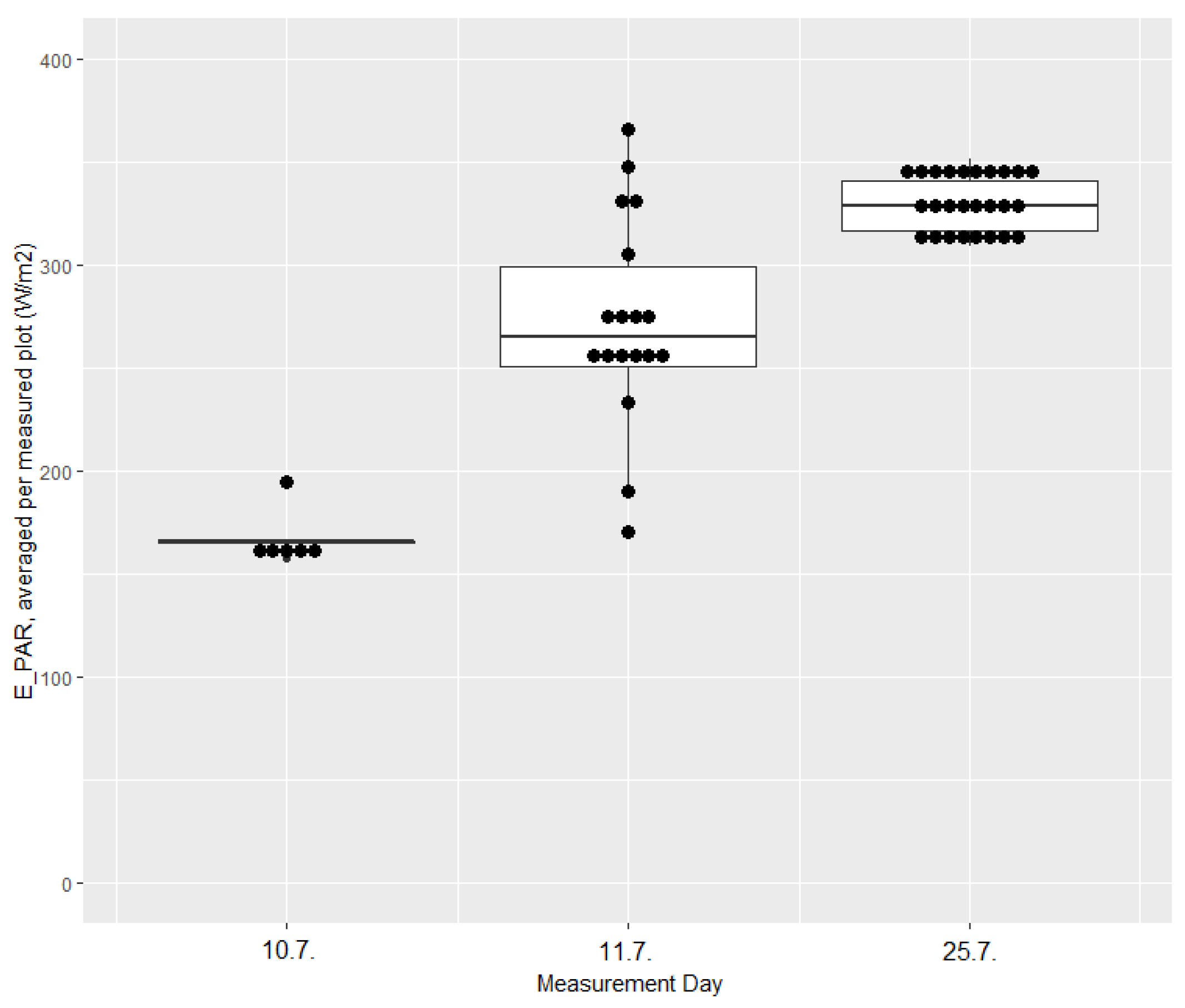
Appendix D. Variation in PAR Values for UAV Measurement Days

Figure A14. Variation in measured E_PAR values for each drone measurement day. Black dots represent individual measuring points.
Remotesensing 15 02498 g0a14

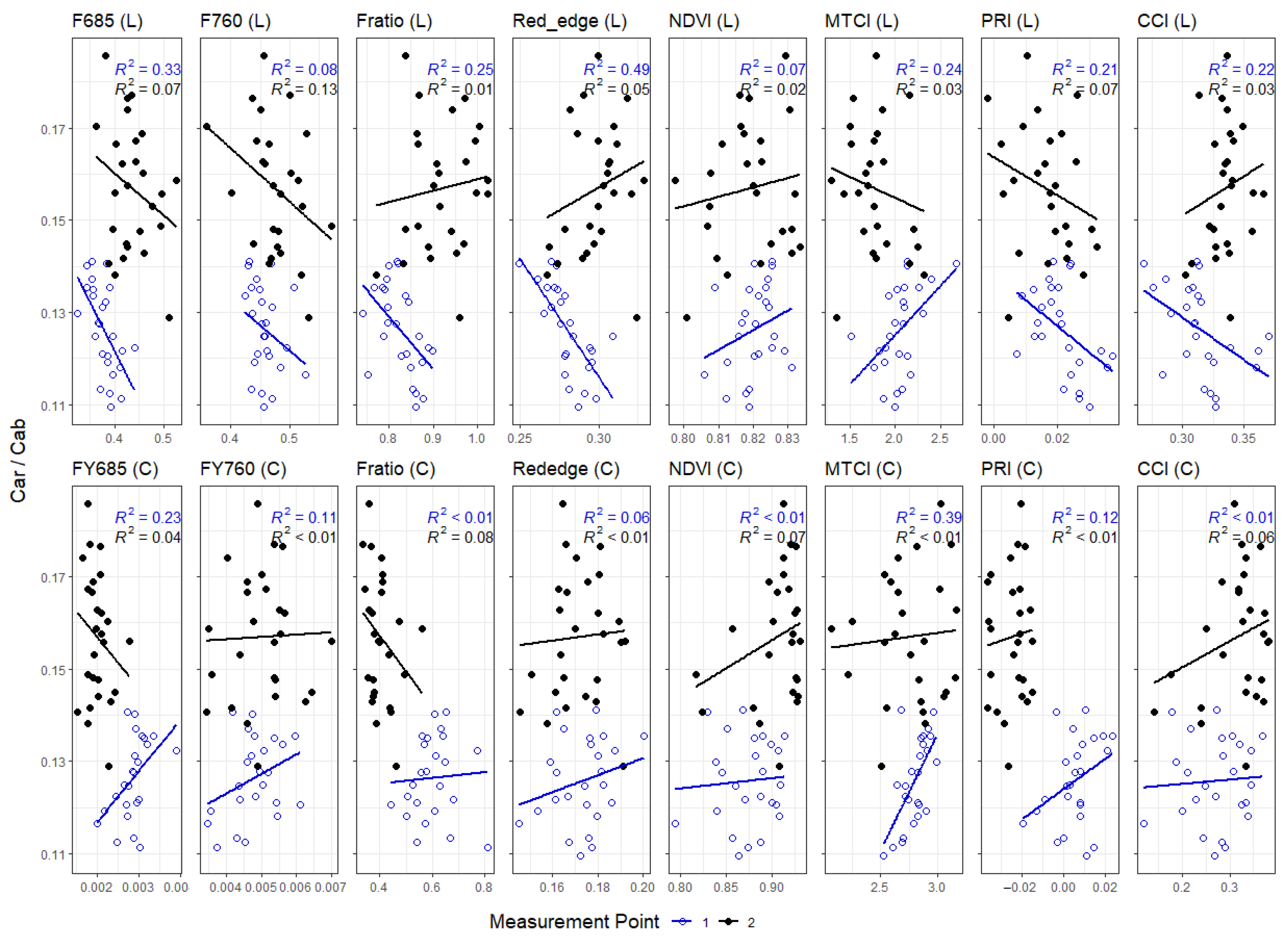
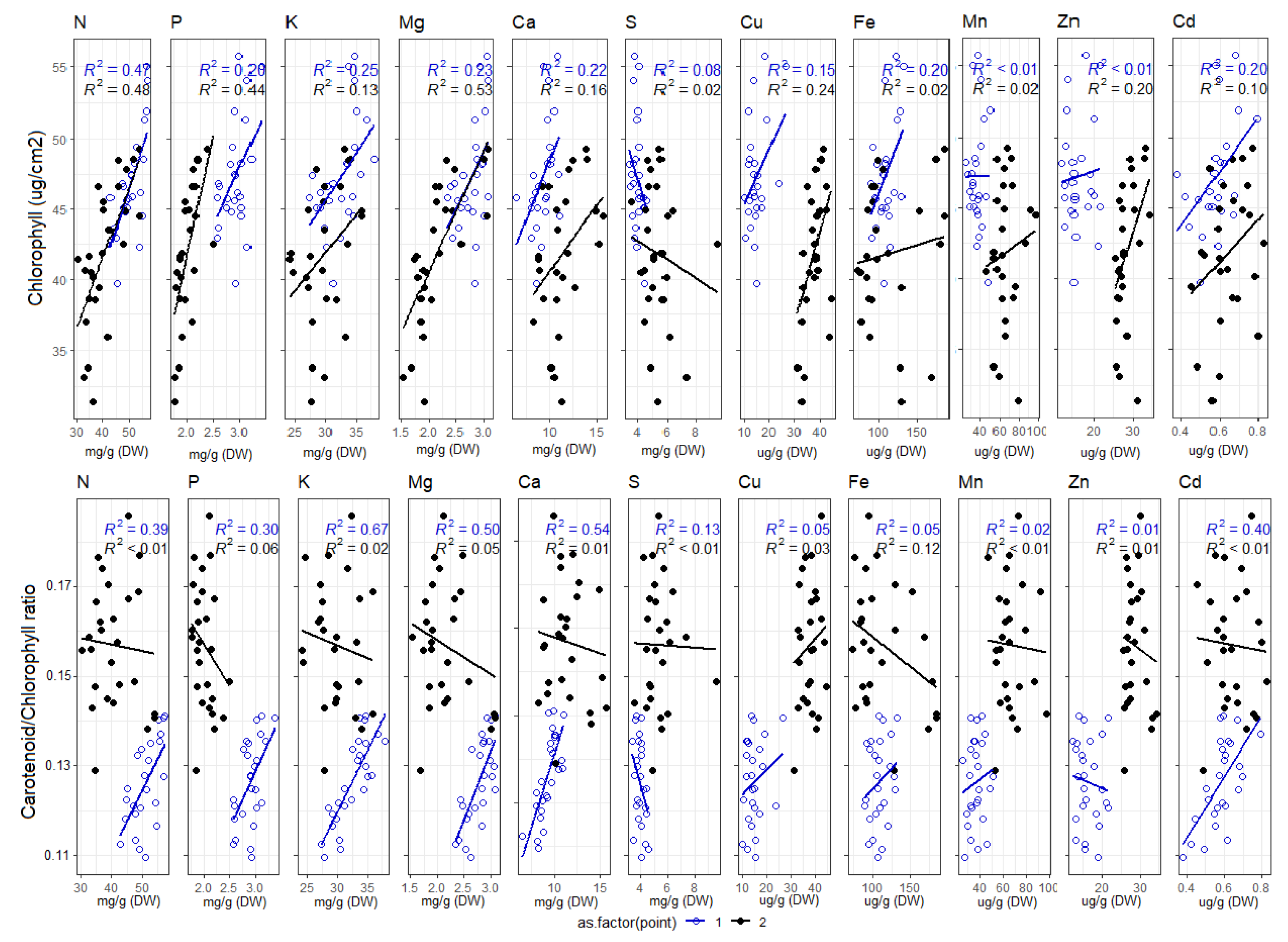
Appendix E. Correlation of Cab and Car/Cab Ratio with Foliar Nutrient Contents, Divided into Early and Late Measurements

Figure A15. Correlation between foliar Cab and nutrients (top row), as well as correlation between the Car/Cab ratio and nutrients (bottom row). Open circles represent measurements from measurement point 1 (n = 26), and closed circles represent measurements from measurement point 2 (n = 26). The R2 values in blue represent the model from the early July measurements, whereas the R2 values in black represent the model from the late July measurements. Some nutrient values are presented as mg/g of dry weight, while others are presented as µg/g dry weight for increased readability.
Remotesensing 15 02498 g0a15

References

  1. Diaz, R.J.; Rosenberg, R. Spreading dead zones and consequences for marine ecosystems. Science 2008, 321, 926–929. [Google Scholar] [CrossRef]
  2. Berry, J.K.; Detgado, J.A.; Khosla, R.; Pierce, F.J. Precision conservation for environmental sustainability. J. Soil Water Conserv. 2003, 58, 332–339. [Google Scholar]
  3. Sishodia, R.P.; Ray, R.L.; Singh, S.K. Applications of remote sensing in precision agriculture: A review. Remote Sens. 2020, 12, 3136. [Google Scholar] [CrossRef]
  4. Muñoz-Huerta, R.F.; Guevara-Gonzalez, R.G.; Contreras-Medina, L.M.; Torres-Pacheco, I.; Prado-Olivarez, J.; Ocampo-Velazquez, R.V. A review of methods for sensing the nitrogen status in plants: Advantages, disadvantages and recent advances. Sensors 2013, 13, 10823–10843. [Google Scholar] [CrossRef] [PubMed] [Green Version]
  5. Hawkesford, M.J.; Cakmak, I.; Coskun, D.; De Kok, L.J.; Lambers, H.; Schjoerring, J.K.; White, P.J. Functions of macronutrients. In Marschner’s Mineral Nutrition of Plants, 2nd ed.; Academic Press: Amsterdam, The Netherlands, 2011; pp. 201–281. [Google Scholar]
  6. Spreitzer, R.J.; Salvucci, M.E. Rubisco: Structure, regulatory interactions, and possibilities for a better enzyme. Annu. Rev. Plant Biol. 2002, 53, 449–475. [Google Scholar] [CrossRef] [Green Version]
  7. Natr, L. Influence of mineral nutrients on photosynthesis of higher plants. Photosynthetica 1972, 6, 80–99. [Google Scholar]
  8. Kalaji, H.M.; Oukarroum, A.; Alexandrov, V.; Kouzmanova, M.; Brestic, M.; Zivcak, M.; Samborska, I.A.; Cetner, M.D.; Allakhverdiev, S.I.; Goltsev, V. Identification of nutrient deficiency in maize and tomato plants by in vivo chlorophyll a fluorescence measurements. Plant Physiol. Biochem. 2014, 81, 16–25. [Google Scholar] [CrossRef]
  9. Osman, K.T. Plant nutrients and soil fertility management. In Soils; Springer: Berlin/Heidelberg, Germany, 2013; pp. 129–159. [Google Scholar]
  10. Lovelock, C.E.; Ball, M.C.; Choat, B.; Engelbrecht, B.M.; Holbrook, N.M.; Feller, I.C. Linking physiological processes with mangrove forest structure: Phosphorus deficiency limits canopy development, hydraulic conductivity and photosynthetic carbon gain in dwarf Rhizophora mangle. Plant Cell Environ. 2006, 29, 793–802. [Google Scholar] [CrossRef] [Green Version]
  11. Rouse, J.W.; Haas, R.H.; Schell, J.A.; Deering, D.W. Monitoring vegetation systems in the Great Plains with ERTS. In Proceedings of the Third Earth Resources Technology Satellite-1 Symp, Greenbelt, MD, USA, 10–15 December 1974; NASA: Washington, DC, USA, 1974; Volume 3, pp. 301–317. [Google Scholar]
  12. Tucker, C.J. Spectral estimation of grass canopy variables. Remote Sens. Environ. 1977, 6, 11–26. [Google Scholar] [CrossRef]
  13. Raun, W.R.; Solie, J.B.; Martin, K.L.; Freeman, K.W.; Stone, M.L.; Johnson, G.V.; Mullen, R.W. Growth stage, development, and spatial variability in corn evaluated using optical sensor readings. J. Plant Nutr. 2005, 28, 173–182. [Google Scholar] [CrossRef]
  14. Vega, F.A.; Ramirez, F.C.; Saiz, M.P.; Rosua, F.O. Multi-temporal imaging using an unmanned aerial vehicle for monitoring a sunflower crop. Biosyst. Eng. 2015, 132, 19–27. [Google Scholar] [CrossRef]
  15. Erdle, K.; Mistele, B.; Schmidhalter, U. Comparison of active and passive spectral sensors in discriminating biomass parameters and nitrogen status in wheat cultivars. Field Crops Res. 2011, 124, 74–84. [Google Scholar] [CrossRef]
  16. Nguy-Robertson, A.; Gitelson, A.; Peng, Y.; Viña, A.; Arkebauer, T.; Rundquist, D. Green leaf area index estimation in maize and soybean: Combining vegetation indices to achieve maximal sensitivity. Agron. J. 2012, 104, 1336–1347. [Google Scholar] [CrossRef] [Green Version]
  17. Dash, J.; Curran, P.J. The MERIS terrestrial chlorophyll index. Int. J. Remote Sens. 2004, 25, 5403–5413. [Google Scholar] [CrossRef]
  18. Li, F.; Miao, Y.; Feng, G.; Yuan, F.; Yue, S.; Gao, X.; Liu, Y.; Liu, B.; Ustin, S.L.; Chen, X. Improving estimation of summer maize nitrogen status with red edge-based spectral vegetation indices. Field Crops Res. 2014, 157, 111–123. [Google Scholar] [CrossRef]
  19. Shiratsuchi, L.; Ferguson, R.; Shanahan, J.; Adamchuk, V.; Rundquist, D.; Marx, D.; Slater, G. Water and nitrogen effects on active canopy sensor vegetation indices. Agron. J. 2011, 103, 1815–1826. [Google Scholar] [CrossRef] [Green Version]
  20. Perez-Priego, O.; Guan, J.; Rossini, M.; Fava, F.; Wutzler, T.; Moreno, G.; Carvalhais, N.; Carrara, A.; Kolle, O.; Julitta, T.; et al. Sun-induced chlorophyll fluorescence and photochemical reflectance index improve remote-sensing gross primary production estimates under varying nutrient availability in a typical Mediterranean savanna ecosystem. Biogeosciences 2015, 12, 6351–6367. [Google Scholar] [CrossRef] [Green Version]
  21. Clevers, J.G.; Kooistra, L. Using hyperspectral remote sensing data for retrieving canopy chlorophyll and nitrogen content. IEEE J. Sel. Top. Appl. Earth Obs. Remote Sens. 2011, 5, 574–583. [Google Scholar] [CrossRef]
  22. Féret, J.B.; Berger, K.; de Boissieu, F.; Malenovský, Z. PROSPECT-PRO for estimating content of nitrogen-containing leaf proteins and other carbon-based constituents. Remote Sens. Environ. 2021, 252, 112173. [Google Scholar] [CrossRef]
  23. Camino, C.; González-Dugo, V.; Hernández, P.; Sillero, J.C.; Zarco-Tejada, P.J. Improved nitrogen retrievals with airborne-derived fluorescence and plant traits quantified from VNIR-SWIR hyperspectral imagery in the context of precision agriculture. Int. J. Appl. Earth Obs. Geoinf. 2018, 70, 105–117. [Google Scholar] [CrossRef]
  24. Berger, K.; Verrelst, J.; Feret, J.B.; Wang, Z.; Wocher, M.; Strathmann, M.; Danner, M.; Mauser, W.; Hank, T. Crop nitrogen monitoring: Recent progress and principal developments in the context of imaging spectroscopy missions. Remote Sens. Environ. 2020, 242, 111758. [Google Scholar] [CrossRef] [PubMed]
  25. Wang, Y.; Suarez, L.; Poblete, T.; Gonzalez-Dugo, V.; Ryu, D.; Zarco-Tejada, P.J. Evaluating the role of solar-induced fluorescence (SIF) and plant physiological traits for leaf nitrogen assessment in almond using airborne hyperspectral imagery. Remote Sens. Environ. 2022, 279, 113141. [Google Scholar] [CrossRef]
  26. Meroni, M.; Rossini, M.; Guanter, L.; Alonso, L.; Rascher, U.; Colombo, R.; Moreno, J. Remote sensing of solar-induced chlorophyll fluorescence: Review of methods and applications. Remote Sens. Environ. 2009, 113, 2037–2051. [Google Scholar] [CrossRef]
  27. Magney, T.S.; Frankenberg, C.; Köhler, P.; North, G.; Davis, T.S.; Dold, C.; Dutta, D.; Fisher, J.B.; Grossmann, K.; Harrington, A.; et al. Disentangling changes in the spectral shape of chlorophyll fluorescence: Implications for remote sensing of photosynthesis. J. Geophys. Res. Biogeosci. 2019, 124, 1491–1507. [Google Scholar] [CrossRef] [Green Version]
  28. Xu, S.; Atherton, J.; Riikonen, A.; Zhang, C.; Oivukkamäki, J.; MacArthur, A.; Honkavaara, E.; Hakala, T.; Koivumäki, N.; Liu, Z.; et al. Structural and photosynthetic dynamics mediate the response of SIF to water stress in a potato crop. Remote Sens. Environ. 2021, 263, 112555. [Google Scholar] [CrossRef]
  29. Porcar-Castell, A.; Tyystjärvi, E.; Atherton, J.; Van der Tol, C.; Flexas, J.; Pfündel, E.E.; Moreno, J.; Frankenberg, C.; Berry, J.A. Linking chlorophyll a fluorescence to photosynthesis for remote sensing applications: Mechanisms and challenges. J. Exp. Bot. 2014, 65, 4065–4095. [Google Scholar] [CrossRef] [Green Version]
  30. Gamon, J.A.; Penuelas, J.; Field, C.B. A narrow-waveband spectral index that tracks diurnal changes in photosynthetic efficiency. Remote Sens. Environ. 1992, 41, 35–44. [Google Scholar] [CrossRef]
  31. Gamon, J.A.; Huemmrich, K.F.; Wong, C.Y.; Ensminger, I.; Garrity, S.; Hollinger, D.Y.; Noormets, A.; Peñuelas, J. A remotely sensed pigment index reveals photosynthetic phenology in evergreen conifers. Proc. Natl. Acad. Sci. USA 2016, 113, 13087–13092. [Google Scholar] [CrossRef] [Green Version]
  32. Wong, C.Y.; D’Odorico, P.; Bhathena, Y.; Arain, M.A.; Ensminger, I. Carotenoid based vegetation indices for accurate monitoring of the phenology of photosynthesis at the leaf-scale in deciduous and evergreen trees. Remote Sens. Environ. 2019, 233, 111407. [Google Scholar] [CrossRef]
  33. Porcar-Castell, A.; Malenovský, Z.; Magney, T.; Van Wittenberghe, S.; Fernández-Marín, B.; Maignan, F.; Zhang, Y.; Maseyk, K.; Atherton, J.; Albert, L.; et al. Chlorophyll a fluorescence illuminates a path connecting plant molecular biology to Earth-system science. Nat. Plants 2021, 7, 998–1009. [Google Scholar] [CrossRef]
  34. Fournier, A.; Daumard, F.; Champagne, S.; Ounis, A.; Goulas, Y.; Moya, I. Effect of canopy structure on sun-induced chlorophyll fluorescence. ISPRS J. Photogramm. Remote Sens. 2012, 68, 112–120. [Google Scholar] [CrossRef]
  35. Gitelson, A.A.; Buschmann, C.; Lichtenthaler, H.K. Leaf chlorophyll fluorescence corrected for re-absorption by means of absorption and reflectance measurements. J. Plant Physiol. 1998, 152, 283–296. [Google Scholar] [CrossRef]
  36. Buschmann, C. Variability and application of the chlorophyll fluorescence emission ratio red/far-red of leaves. Photosynth. Res. 2007, 92, 261–271. [Google Scholar] [CrossRef]
  37. Liu, W.; Atherton, J.; Mõttus, M.; Gastellu-Etchegorry, J.P.; Malenovský, Z.; Raumonen, P.; Åkerblom, M.; Mäkipää, R.; Porcar-Castell, A. Simulating solar-induced chlorophyll fluorescence in a boreal forest stand reconstructed from terrestrial laser scanning measurements. Remote Sens. Environ. 2019, 232, 111274. [Google Scholar] [CrossRef]
  38. Zarco-Tejada, P.J.; Berni, J.A.; Suárez, L.; Sepulcre-Cantó, G.; Morales, F.; Miller, J.R. Imaging chlorophyll fluorescence with an airborne narrow-band multispectral camera for vegetation stress detection. Remote Sens. Environ. 2009, 113, 1262–1275. [Google Scholar] [CrossRef]
  39. Rossini, M.; Nedbal, L.; Guanter, L.; Ač, A.; Alonso, L.; Burkart, A.; Cogliati, S.; Colombo, R.; Damm, A.; Drusch, M.; et al. Red and far red Sun-induced chlorophyll fluorescence as a measure of plant photosynthesis. Geophys. Res. Lett. 2015, 42, 1632–1639. [Google Scholar] [CrossRef] [Green Version]
  40. Wood, J.D.; Griffis, T.J.; Baker, J.M.; Frankenberg, C.; Verma, M.; Yuen, K. Multi-scale analyses reveal robust relationships between gross primary production and solar induced fluorescence. Geophys. Res. Lett. 2016, 44, 533–541. [Google Scholar] [CrossRef]
  41. Cendrero-Mateo, M.P.; Wieneke, S.; Damm, A.; Alonso, L.; Pinto, F.; Moreno, J.; Guanter, L.; Celesti, M.; Rossini, M.; Sabater, N.; et al. Sun-induced chlorophyll fluorescence III: Benchmarking retrieval methods and sensor characteristics for proximal sensing. Remote Sens. 2019, 11, 962. [Google Scholar] [CrossRef] [Green Version]
  42. Zeng, Y.; Badgley, G.; Dechant, B.; Ryu, Y.; Chen, M.; Berry, J.A. A practical approach for estimating the escape ratio of near-infrared solar-induced chlorophyll fluorescence. Remote Sens. Environ. 2019, 232, 111209. [Google Scholar] [CrossRef] [Green Version]
  43. Jia, M.; Zhu, J.; Ma, C.; Alonso, L.; Li, D.; Cheng, T.; Tian, Y.; Zhu, Y.; Yao, X.; Cao, W. Difference and potential of the upward and downward sun-induced chlorophyll fluorescence on detecting leaf nitrogen concentration in wheat. Remote Sens. 2018, 10, 1315. [Google Scholar] [CrossRef] [Green Version]
  44. Jia, M.; Colombo, R.; Rossini, M.; Celesti, M.; Zhu, J.; Cogliati, S.; Cheng, T.; Tian, Y.; Zhu, Y.; Cao, W.; et al. Estimation of leaf nitrogen content and photosynthetic nitrogen use efficiency in wheat using sun-induced chlorophyll fluorescence at the leaf and canopy scales. Eur. J. Agron. 2021, 122, 126192. [Google Scholar] [CrossRef]
  45. Peñuelas, J.; Gamon, J.A.; Fredeen, A.L.; Merino, J.; Field, C.B. Reflectance indices associated with physiological changes in nitrogen-and water-limited sunflower leaves. Remote Sens. Environ. 1994, 48, 135–146. [Google Scholar] [CrossRef]
  46. Moran, J.A.; Mitchell, A.K.; Goodmanson, G.; Stockburger, K.A. Differentiation among effects of nitrogen fertilization treatments on conifer seedlings by foliar reflectance: A comparison of methods. Tree Physiol. 2000, 20, 1113–1120. [Google Scholar] [CrossRef] [Green Version]
  47. Gamon, J.; Serrano, L.; Surfus, J.S. The photochemical reflectance index: An optical indicator of photosynthetic radiation use efficiency across species, functional types, and nutrient levels. Oecologia 1997, 112, 492–501. [Google Scholar] [CrossRef] [PubMed]
  48. Xu, X.G.; Zhao, C.J.; Wang, J.H.; Zhang, J.C.; Song, X.Y. Using optimal combination method and in situ hyperspectral measurements to estimate leaf nitrogen concentration in barley. Precis. Agric. 2014, 15, 227–240. [Google Scholar] [CrossRef]
  49. Kawamura, K.; Mackay, A.D.; Tuohy, M.P.; Betteridge, K.; Sanches, I.D.; Inoue, Y. Potential for spectral indices to remotely sense phosphorus and potassium content of legume-based pasture as a means of assessing soil phosphorus and potassium fertility status. Int. J. Remote Sens. 2011, 32, 103–124. [Google Scholar] [CrossRef]
  50. Rajewicz, P.A.; Atherton, J.; Alonso, L.; Porcar-Castell, A. Leaf-level spectral fluorescence measurements: Comparing methodologies for broadleaves and needles. Remote Sens. 2019, 11, 532. [Google Scholar] [CrossRef] [Green Version]
  51. Olascoaga, B.; Mac Arthur, A.; Atherton, J.; Porcar-Castell, A. A comparison of methods to estimate photosynthetic light absorption in leaves with contrasting morphology. Tree Physiol. 2016, 36, 368–379. [Google Scholar] [CrossRef] [Green Version]
  52. Dash, J.; Curran, P.J. Evaluation of the MERIS terrestrial chlorophyll index (MTCI). Adv. Space Res. 2007, 39, 100–104. [Google Scholar] [CrossRef]
  53. Horler, D.N.H.; Dockray, M.; Barber, J. The red edge of plant leaf reflectance. Int. J. Remote Sens. 1983, 4, 273–288. [Google Scholar] [CrossRef]
  54. Thomas, R. Practical Guide to ICP-MS: A Tutorial for Beginners, 2nd ed.; CRC Press: Boca Raton, FL, USA, 2003. [Google Scholar]
  55. Bremner, J.M. Nitrogen-total. In Methods of Soil Analysis: Part 3 Chemical Methods, 5; American Society of Agronomy: Madison, WI, USA, 1996; pp. 1085–1121. [Google Scholar]
  56. Wellburn, A.R. The spectral determination of chlorophylls a and b, as well as total carotenoids, using various solvents with spectrophotometers of different resolution. J. Plant Physiol. 1994, 144, 307–313. [Google Scholar] [CrossRef]
  57. MacArthur, A.; Robinson, I.; Rossini, M.; Davis, N.; MacDonald, K. A dual-field-of-view spectrometer system for reflectance and fluorescence measurements (Piccolo Doppio) and correction of etaloning. In Fifth International Workshop on Remote Sensing of Vegetation Fluorescence; European Space Agenccy: Paris, France, 2014. [Google Scholar]
  58. Atherton, J.; MacArthur, A.; Hakala, T.; Maseyk, K.; Robinson, I.; Liu, W.; Honkavaara, E.; Porcar-Castell, A. Drone measurements of solar-induced chlorophyll fluorescence acquired with a low-weight DFOV spectrometer system. In Proceedings of the IGARSS 2018—2018 IEEE International Geoscience and Remote Sensing Symposium, Valencia, Spain, 22–27 July 2018; pp. 8834–8836. [Google Scholar]
  59. Vargas, J.Q.; Bendig, J.; Mac Arthur, A.; Burkart, A.; Julitta, T.; Maseyk, K.; Thomas, R.; Siegmann, B.; Rossini, M.; Celesti, M.; et al. Unmanned aerial systems (UAS)-based methods for solar induced chlorophyll fluorescence (SIF) retrieval with non-imaging spectrometers: State of the art. Remote Sens. 2020, 12, 1624. [Google Scholar] [CrossRef]
  60. Meroni, M.; Busetto, L.; Colombo, R.; Guanter, L.; Moreno, J.; Verhoef, W. Performance of spectral fitting methods for vegetation fluorescence quantification. Remote Sens. Environ. 2010, 114, 363–374. [Google Scholar] [CrossRef]
  61. Gitelson, A.A.; Kaufman, Y.J.; Stark, R.; Rundquist, D. Novel algorithms for remote estimation of vegetation fraction. Remote Sens. Environ. 2002, 80, 76–87. [Google Scholar] [CrossRef] [Green Version]
  62. Munné-Bosch, S.; Alegre, L. Die and let live: Leaf senescence contributes to plant survival under drought stress. Funct. Plant Biol. 2004, 31, 203–216. [Google Scholar] [CrossRef]
  63. Gómez, M.I.; Magnitskiy, S.; Rodríguez, L.E. Critical dilution curves for nitrogen, phosphorus, and potassium in potato group Andigenum. Agron. J. 2019, 111, 419–427. [Google Scholar] [CrossRef]
  64. Lambers, H.; Oliveira, R.S. Plant Nutrient Use Efficiency. Mineral nutrition. In Plant Physiological Ecology; Springer: Berlin/Heidelberg, Germany, 2019; pp. 301–384. [Google Scholar]
  65. Abukmeil, R.; Al-Mallahi, A.A.; Campelo, F. New approach to estimate macro and micronutrients in potato plants based on foliar spectral reflectance. Comput. Electron. Agric. 2022, 198, 107074. [Google Scholar] [CrossRef]
  66. Lizarazo, C.I.; Yli-Halla, M.; Stoddard, F.L. Pre-crop effects on the nutrient composition and utilization efficiency of faba bean (Vicia faba L.) and narrow-leafed lupin (Lupinus angustifolius L.). Nutr. Cycl. Agroecosyst. 2015, 103, 311–327. [Google Scholar] [CrossRef]
  67. Evans, J.R. Photosynthesis and nitrogen relationships in leaves of C3 plants. Oecologia 1989, 78, 9–19. [Google Scholar] [CrossRef]
  68. Reich, P.B.; Walters, M.B.; Kloeppel, B.D.; Ellsworth, D.S. Different photosynthesis-nitrogen relations in deciduous hardwood and evergreen coniferous tree species. Oecologia 1995, 104, 24–30. [Google Scholar] [CrossRef] [PubMed]
  69. Hawkesford, M.; Horst, W.; Kichey, T.; Lambers, H.; Schjoerring, J.; Møller, I.S.; White, P. Functions of macronutrients. In Marschner’s Mineral Nutrition of Higher Plants; Academic Press: Amsterdam, The Netherlands, 2021; pp. 135–189. [Google Scholar]
  70. Pätsikkä, E.; Kairavuo, M.; Šeršen, F.; Aro, E.M.; Tyystjärvi, E. Excess copper predisposes photosystem II to photoinhibition in vivo by outcompeting iron and causing decrease in leaf chlorophyll. Plant Physiol. 2002, 129, 1359–1367. [Google Scholar] [CrossRef] [PubMed] [Green Version]
  71. Burke, J.J.; Holloway, P.; Dalling, M.J. The effect of sulfur deficiency on the organisation and photosynthetic capability of wheat leaves. J. Plant Physiol. 1986, 125, 371–375. [Google Scholar] [CrossRef]
  72. Hu, H.; Sparks, D. Zinc Deficiency Inhibits Chlorophyll Synthesis and Gas Exchange in Stuart Pecan. Hort. Sci. 1991, 26, 267–268. [Google Scholar] [CrossRef] [Green Version]
  73. Shenker, M.; Plessner, O.E.; Tel-Or, E. Manganese nutrition effects on tomato growth, chlorophyll concentration, and superoxide dismutase activity. J. Plant Physiol. 2004, 161, 197–202. [Google Scholar] [CrossRef]
  74. Gitelson, A.A.; Kaufman, Y.J.; Merzlyak, M.N. Use of a green channel in remote sensing of global vegetation from EOS-MODIS. Remote Sens. Environ. 1996, 58, 289–298. [Google Scholar] [CrossRef]
  75. Satognon, F.; Lelei, J.J.; Owido, S.F. Use of GreenSeeker and CM-100 as manual tools for nitrogen management and yield prediction in irrigated potato (Solanum tuberosum) production. Arch. Agric. Environ. Sci. 2021, 6, 121–128. [Google Scholar] [CrossRef]
  76. Filella, I.; Penuelas, J. The red edge position and shape as indicators of plant chlorophyll content, biomass and hydric status. Int. J. Remote Sens. 1994, 15, 1459–1470. [Google Scholar] [CrossRef]
  77. Kanke, Y.; Raun, W.; Solie, J.; Stone, M.; Taylor, R. Red edge as a potential index for detecting differences in plant nitrogen status in winter wheat. J. Plant Nutr. 2012, 35, 1526–1541. [Google Scholar] [CrossRef]
  78. Fridgen, J.L.; Varco, J.J. Dependency of cotton leaf nitrogen, chlorophyll, and reflectance on nitrogen and potassium availability. Agron. J. 2004, 96, 63–69. [Google Scholar] [CrossRef]
  79. Choudhury, M.R.; Christopher, J.; Das, S.; Apan, A.; Menzies, N.W.; Chapman, S.; Mellro, V.; Dang, Y.P. Detection of calcium, magnesium, and chlorophyll variations of wheat genotypes on sodic soils using hyperspectral red edge parameters. Environ. Technol. Innov. 2022, 27, 102469. [Google Scholar] [CrossRef]
  80. Agati, G.; Foschi, L.; Grossi, N.; Guglielminetti, L.; Cerovic, Z.G.; Volterrani, M. Fluorescence-based versus reflectance proximal sensing of nitrogen content in Paspalum vaginatum and Zoysia matrella turfgrasses. Eur. J. Agron. 2013, 45, 39–51. [Google Scholar] [CrossRef]
  81. Ač, A.; Malenovský, Z.; Olejníčková, J.; Gallé, A.; Rascher, U.; Mohammed, G. Meta-analysis assessing potential of steady-state chlorophyll fluorescence for remote sensing detection of plant water, temperature and nitrogen stress. Remote Sens. Environ. 2015, 168, 420–436. [Google Scholar] [CrossRef] [Green Version]
  82. Filella, I.; Porcar-Castell, A.; Munné-Bosch, S.; Bäck, J.; Garbulsky, M.F.; Peñuelas, J. PRI assessment of long-term changes in carotenoids/chlorophyll ratio and short-term changes in de-epoxidation state of the xanthophyll cycle. Int. J. Remote Sens. 2009, 30, 4443–4455. [Google Scholar] [CrossRef]
  83. Gitelson, A.A.; Gamon, J.A.; Solovchenko, A. Multiple drivers of seasonal change in PRI: Implications for photosynthesis 1. Leaf level. Remote Sens. Environ. 2017, 191, 110–116. [Google Scholar] [CrossRef] [Green Version]
  84. Jongschaap, R.E.; Booij, R. Spectral measurements at different spatial scales in potato: Relating leaf, plant and canopy nitrogen status. Int. J. Appl. Earth Obs. Geoinf. 2004, 5, 205–218. [Google Scholar] [CrossRef]
  85. Gara, T.W.; Skidmore, A.K.; Darvishzadeh, R.; Wang, T. Leaf to canopy upscaling approach affects the estimation of canopy traits. GIScience Remote Sens. 2019, 56, 554–575. [Google Scholar] [CrossRef]
  86. Nigon, T.J.; Mulla, D.J.; Rosen, C.J.; Cohen, Y.; Alchanatis, V.; Knight, J.; Rud, R. Hyperspectral aerial imagery for detecting nitrogen stress in two potato cultivars. Comput. Electron. Agric. 2015, 112, 36–46. [Google Scholar] [CrossRef]
  87. Atherton, J.; Zhang, C.; Oivukkamäki, J.; Kulmala, L.; Xu, S.; Hakala, T.; Honkavaara, E.; MacArthur, A.; Porcar-Castell, A. What does the NDVI really tell us about crops? Insight from proximal spectral field sensors. In Information and Communication Technologies for Agriculture—Theme I: Sensors; Springer: Berlin/Heidelberg, Germany, 2022; pp. 251–265. [Google Scholar]
  88. Verrelst, J.; Rivera, J.P.; van der Tol, C.; Magnani, F.; Mohammed, G.; Moreno, J. Global sensitivity analysis of the SCOPE model: What drives simulated canopy-leaving sun-induced fluorescence? Remote Sens. Environ. 2015, 166, 8–21. [Google Scholar] [CrossRef]
  89. Gitelson, A.A.; Gamon, J.A.; Solovchenko, A. Multiple drivers of seasonal change in PRI: Implications for photosynthesis 2. Stand level. Remote Sens. Environ. 2017, 190, 198–206. [Google Scholar] [CrossRef] [Green Version]
  90. Lu, B.; Dao, P.D.; Liu, J.; He, Y.; Shang, J. Recent advances of hyperspectral imaging technology and applications in agriculture. Remote Sens. 2020, 12, 2659. [Google Scholar] [CrossRef]
  91. Ye, X.; Abe, S.; Zhang, S. Estimation and mapping of nitrogen content in apple trees at leaf and canopy levels using hyperspectral imaging. Precis. Agric. 2020, 21, 198–225. [Google Scholar] [CrossRef]
Figure 1. Experimental setup and meteorological data. Panel (A) shows measurement plots during early (10.7) and late season measurements (25.7) with specific plots marked with white color. Photo taken from a UAV using a MicaSense RedEdge M camera. Nutrient treatments are enclosed in the green box, and water stress treatments are in the blue box. Panel (B) shows micrometeorological conditions during the measurement campaign, showing daily mean temperatures with daily mean precipitation in Helsinki, July 2018. Panel (C) shows a photographic example of the fully developed potato plant canopy.
Remotesensing 15 02498 g001
Figure 2. Experimental setup and underlying logic of the study. The dynamics of leaf and canopy-level traits in response to fertilization, water stress, and canopy development were measured. Subsequently, we characterize the relationships between leaf and canopy-level traits and spectral indices, investigating and discussing the mechanisms that underlie the relationships at each scale.
Remotesensing 15 02498 g002
Figure 3. Examples of measured leaf-level fluorescence and reflectance spectra with selected indices. In (A), a typical example of the spectral fluorescence spectrum is shown with fluorescence peaks and oxygen bands marked. In (B), a typical leaf reflectance spectrum depicts the reflectance indices selected in this study.
Remotesensing 15 02498 g003
Figure 4. Macro- (A) and micronutrient (B) levels in the early and late measurements arranged by treatments. Coloured bars signify different treatments, grouped by measurement point. Black bars signify the standard deviation. Small letters denote significant differences between treatment groups (p < 0.05) for that specific nutrient. For example, the bars with the letter “a” are not significantly different from each other but are significantly different from the bars with the letter “b”. Stars denote significant differences between early and late measurements for each treatment group (p < 0.05) (n = 4 in the fertilization experiment, n = 5 in the water stress experiment).
Remotesensing 15 02498 g004
Figure 5. Specific leaf area (SLA), total chlorophyll (Cab), and carotenoid-chlorophyll ratio (Car/Cab) across treatments and measurement period. Coloured bars signify different treatments, grouped by nutrient and measurement point. Black bars signify the standard deviation. Small letters denote significant differences between treatment groups (p < 0.05). For example, all the bars with the letter “a” are not significantly different from each other but are significantly different from the bars with the letter “b”. Stars denote significant differences between the early and late measurements for each treatment group (p < 0.05) (n = 4 in the fertilization experiment and n = 5 in the water stress experiment).
Remotesensing 15 02498 g005
Figure 6. Fractional vegetation cover (FVC). Spatial and temporal variation in vegetation fraction, calculated from canopy level multispectral UAV data using the NIR-band. Colored bars signify different treatments, grouped by nutrient and measurement point. Black bars signify the standard deviation. Changes in treatments between early and late measurements were not significant. n = 4 in nutrient studies and n = 5 in the water stress experiment. A horizontal line has been added (FVC = 0.75) to facilitate comparison of early and late measurements.
Remotesensing 15 02498 g006
Figure 7. Correlation matrix comparing leaf (L) and canopy (C) level spectral indices to leaf level nutrient and pigment contents. If the color of the correlation between the leaf and canopy stays the same, it indicates that the sign of the correlation scales up. If the color changes between the scales, the correlation is reversed when moving from one scale to another. The data used in the matrix is a combination of early and late measurement points (n = 52). Color denotes the Pearson correlation coefficient R-value, which is explained in the color chart on the right. All colored (non-white) squares are significant at the p ≤ 0.05 level.
Remotesensing 15 02498 g007
Figure 8. Correlation between foliar Cab contents and spectral indices at the leaf level and the canopy scale. Open circles represent measurements from measurement point 1 (n = 26), and closed circles represent measurements from measurement point 2 (n = 26). The top row of data represents the leaf level spectral measurements, and the bottom row of data represents the canopy measurements. The R2 values in blue represent the model from the early July measurements, whereas the R2 values in black represent the model from the late July measurements. A red linear correlation line in the plot (together with a R2 value), indicates that the models from individual measurement points are not significantly different from the model that includes data from both early and late measurements.
Remotesensing 15 02498 g008
Figure 9. Detecting leaf N contents with spectral indices at the leaf level and the canopy scale. Open circles represent measurements from measurement point 1 (n = 26), and closed circles represent measurements from measurement point 2 (n = 26). The top row of data represents the leaf level spectral indices, and the bottom row of data represents the canopy measurements. The R2 values in blue represent the model from the early July measurements, whereas the R2 values in black represent the model from the late July measurements. A red linear correlation line in the plot (together with a R2 value) indicates that the models from individual measurements are not significantly different from the model that includes data from both measurements.
Remotesensing 15 02498 g009
Table 1. Macro- and micronutrients targeted in this study and their primary functions in plants.
NutrientFunction in Plant
NRequired for all proteins, e.g., RuBisCO, chlorophyll synthesis, electron transport
PEssential for cellular energy transfer and metabolism: ATP and NADP
KPhotosynthesis (through ATP synthesis) and stomatal control
MgChlorophyll synthesis, phosphate metabolism, protein (e.g., ATP) activation
CaCell wall synthesis, acts as a messenger in nutrient and stress signaling in plant
SAmino acid (cysteine and methionine) and coenzyme synthesis
CuProtein synthesis (e.g., plastocyanin), nitrogen fixation
FeChlorophyll synthesis and chloroplast maintenance
MnMetabolic processes (glycosylation) and nitrogen assimilation
ZnRegulates plant response to biotic and abiotic stress, protein synthesis
CdNon-essential, hinders nutrient and water uptake
Table 2. Dosification in each of the fertilization treatments (Kg/ha).
Nutrient Doses per Treatment (kg/ha)
N1A1N2A0N2A1CONTROL N2A2
N32.565.065.065.0
P13.60.013.627.2
K53.22.454.4106.4
Mg4.72.45.99.5
S29.59.634.459.1
B0.10.00.20.3
Cu0.10.00.10.2
Fe0.20.00.20.5
Mn0.70.00.71.5
Zn0.10.00.10.2
Table 3. Vegetation indices used in this study. R denotes reflectance, and the number corresponds to the wavelength in nanometers.
Vegetation IndexEquationReference
NDVI N D V I = R 860 R 660 R 860 + R 660 Rouse et al. [11]
MTCI M T C I = R 753 R 709 R 709 R 681 Dash and Curran [52]
Red edge R e d   e d g e = R 712 nm 722 nm Horler et al. [53]
PRI P R I = R 531 R 570 R 531 + R 570 Gamon et al. [30]
CCI C C I = R 531 R 645 R 531 + R 645 Gamon et al. [31]
Disclaimer/Publisher’s Note: The statements, opinions and data contained in all publications are solely those of the individual author(s) and contributor(s) and not of MDPI and/or the editor(s). MDPI and/or the editor(s) disclaim responsibility for any injury to people or property resulting from any ideas, methods, instructions or products referred to in the content.

