Article

A Unified Physically Based Method for Monitoring Grassland Nitrogen Concentration with Landsat 7, Landsat 8, and Sentinel-2 Satellite Data

by
Mohammad Hossain Dehghan-Shoar
1,2,*,
Reddy R. Pullanagari
2,
Gabor Kereszturi
1,
Alvaro A. Orsi
3,
Ian J. Yule
2 and
James Hanly
1
1
School of Agriculture and Environment, Massey University, Tennent Drive, Palmerston North 4414, New Zealand
2
Stoneleigh Consulting Limited, 70a Francis Road, Whakamarama, Western Bay Of Plenty, Bay of Plenty 3172, New Zealand
3
Institute of Environmental Science and Research Limited (ESR), Mt Albert Science Centre, 120 Mt Albert Road, Auckland 1025, New Zealand
*
Author to whom correspondence should be addressed.
Remote Sens. 2023, 15(10), 2491; https://doi.org/10.3390/rs15102491
Submission received: 13 March 2023 / Revised: 20 April 2023 / Accepted: 6 May 2023 / Published: 9 May 2023
(This article belongs to the Special Issue Remote Sensing of Vegetation Biochemical and Biophysical Parameters)

Abstract

:
The increasing number of satellite missions provides vast opportunities for continuous vegetation monitoring, crucial for precision agriculture and environmental sustainability. However, accurately estimating vegetation traits, such as nitrogen concentration (N%), from Landsat 7 (L7), Landsat 8 (L8), and Sentinel-2 (S2) satellite data is challenging due to the diverse sensor configurations and complex atmospheric interactions. To address these limitations, we developed a unified and physically based method that combines a soil–plant–atmosphere radiative transfer (SPART) model with the bottom-of-atmosphere (BOA) spectral bidirectional reflectance distribution function. This approach enables us to assess the effect of rugged terrain, viewing angles, and illumination geometry on the spectral reflectance of multiple sensors. Our methodology involves inverting radiative transfer model variables using numerical optimization to estimate N% and creating a hybrid model. We used Gaussian process regression (GPR) to incorporate the inverted variables into the hybrid model for N% prediction, resulting in a unified approach for N% estimation across different sensors. Our model shows a validation accuracy of 0.35 (RMSE %N), a mean prediction interval width (MPIW) of 0.35, and an R 2 of 0.50, using independent data from multiple sensors collected between 2016 and 2019. Our unified method provides a promising solution for estimating N% in vegetation from L7, L8, and S2 satellite data, overcoming the limitations posed by diverse sensor configurations and complex atmospheric interactions.

1. Introduction

Grassland productivity is critical for the meat and dairy sectors due to the ever-increasing demand for high-quality meat and dairy products [1]. As a significant component of the vegetation photosynthetic apparatus, nitrogen concentration (N%) plays a crucial role in grassland productivity. Nitrogen-based chemical fertilizers are commonly applied to grasslands to increase productivity, which can harm the environment [2,3,4]. Therefore, optimizing the application of nitrogen chemical fertilizers to grasslands is essential. Traditionally, grassland N% is monitored by collecting grass samples and sending them to a chemical lab for wet chemistry analysis. An alternative method of monitoring grassland N% is using spaceborne optical imagery [5,6,7,8]. Spaceborne optical imagery measures the electromagnetic radiation flux reflected by the incident solar radiation of a surface, commonly referred to as reflectance.
Reflectance is the ratio of the amount of light reflected from a surface to the amount of incident light. Vegetation has a unique reflectance profile across different wavelengths of the electromagnetic spectrum, allowing for the identification of specific chemical properties, including N%, which could be detected using the visible (VIS), near infrared (NIR), and short wave infrared (SWIR) regions of the spectrum [9]. Reflectance can be categorized into top of atmosphere (TOA) and top of canopy (TOC) reflectance [10,11]. TOA reflectance represents the measurements of the electromagnetic radiation flux reflected by the earth’s surface and atmosphere. Although it includes atmospheric effects that may distort the actual reflectance profile of the vegetation, TOA reflectance is widely used in remote sensing applications due to its accessibility and global coverage [12]. By applying atmospheric correction techniques, TOA reflectance data can be converted to TOC reflectance, which refers to the measurements of the radiation flux reflected only by the earth’s surface, excluding atmospheric effects [13]. TOC reflectance is considered more relevant for studying vegetation properties, such as N%, because it provides a more accurate representation of the actual reflectance profile of the vegetation by minimizing atmospheric interference [14]. However, the use of TOA reflectance in combination with appropriate atmospheric correction methods can still provide valuable information for monitoring grassland productivity and optimizing nitrogen fertilizer application.
The presence of chlorophyll and protein content, which are closely associated with N%, results in distinct spectral reflection that can be detected by spaceborne optical instruments [9,15,16,17,18]. By analyzing these spectral signatures and the associated reflectance values, it is possible to estimate the N% of vegetation. Advanced algorithms and models are developed to interpret these spectral data and derive accurate N% estimations. This method allows for the non-destructive and continuous monitoring of N% at large spatial scales, making it more efficient than traditional sampling methods [19]. By leveraging the unique reflectance properties of vegetation and advanced data processing techniques, optical remote sensing provides an effective alternative for monitoring grassland N%.
Monitoring N% in grasslands using spaceborne optical imagery faces significant challenges, including cloud coverage and image acquisition frequency. One solution to address these issues is to utilize a combination of multiple optical sensors, such as Landsat 7 (L7), Landsat 8 (L8), and Sentinel-2 (S2), for continuous and comprehensive monitoring. These sensors provide a robust monitoring solution by increasing the data sample size and offering more frequent images. For example, L7 features a 16-day revisit time, L8 has a 16-day revisit time on the same path and a 5-day revisit time on adjacent paths, while S2 has a 5-day revisit time [20,21,22]. Leveraging multiple sensors with varying revisit times minimizes the impact of cloud coverage or poor image quality on any individual image. However, effectively using the interchangeability of these sensors still needs to be improved. First, each sensor has unique spectral and spatial resolutions and radiometric calibration, leading to inconsistencies when merging data from different sources [23]. Preprocessing and normalization are required to ensure accurate and comparable results. Second, the varying revisit times of these sensors can result in temporal mismatches, making it challenging to create a seamless time series of observations [24]. Innovative methodologies and tools to fully exploit the potential of using multiple optical sensors for N% monitoring in grasslands must be developed to overcome these challenges.
A common approach to tackling this issue is through a sensor harmonization process called the bi-directional reflectance distribution function (BRDF) [25,26]. BRDF accounts for the directional dependence of a target’s reflected energy as a function of illumination and viewing geometries, producing cross-sensor consistent surface reflectance products [27,28]. By converting the imagery to the earth’s surface point directly below the satellite and considering factors such as incidence and reflected zenith and azimuth angles, wavelength, and spectral irradiance, BRDF enables the continuous monitoring of grasslands’ biochemical and biophysical properties, including N%. Although BRDF is a powerful solution, it can be computationally demanding due to its wavelength dependence and may pose challenges when used with sensors featuring numerous spectral bands [29]. Despite these hurdles, integrating multiple optical sensors with BRDF presents a promising strategy for overcoming cloud coverage and image acquisition time challenges in grassland N% monitoring [27].
In grassland monitoring, topography presents a significant challenge [30]. Its influence on spectral imagery is often underestimated, yet topography plays a crucial role in the spectral analysis of vegetation in an uneven terrain [31,32,33]. This is because areas with slopes facing the light source receive more significant amounts of down-welling radiation, resulting in increased illumination [34]. Consequently, this hinders the accurate retrieval of biochemical and biophysical properties of vegetation using empirical–statistical- or physically based methods. Moreover, the anisotropic nature of non-Lambertian surfaces adds complexity, as the radiance detected by the observing sensor is further influenced by surface characteristics [35,36].
Many topographical correction methods have been developed for Lambertian and non-Lambertian surfaces [37]. A common method of undertaking topographical correction is by using the cosine method. This method uses the linear relationship between the radiance measured and the viewing incident angle to undertake topographical correction [38,39]. However, this method has certain limitations, such as the fact that it does not consider the impact of diffuse irradiance. To address these limitations of the cosine method, Gu and Gillespie [32] proposed using the sun–canopy–sensor (SCS) topographic correction method, which accounts for some BRDF effects over rugged terrain. This method improves upon the cosine correction method by normalizing the illuminated canopy area of a scene. However, as the SCS method does not consider the impact of diffuse irradiance, this topographic correction technique may result in over-correction for slopes facing away from the sun. To address this limitation of the SCS method, Soenen et al. [40] proposed a moderator variable (C) that simulates the effect of diffuse sky illumination. This variable is derived by calculating the linear relationship between the radiance and cosine of the incidence angle Gu and Gillespie [32], Soenen et al. [40].
Estimating the biochemical and biophysical properties of vegetation can be achieved using physically based RTMs [11,41]. These models monitor the vegetation properties by simulating the interaction between incoming solar radiation and vegetative canopies [10,42,43,44,45]. One approach involves variable inversion, where RTMs simulate the observed reflectance spectrum as a function of several biophysical and biochemical variables, such as leaf area index (LAI), protein content (Cp), and chlorophyll content (Cab) [46,47,48]. Inverting these variables allows RTMs to find the best match between measured and predicted spectra. Accurately and reliably inverting the biochemical and biophysical variables of RTMs is challenging due to the ill-posed nature of RTM problems and our limited understanding of the biophysical processes governing photon scattering, absorption, and transmission when interacting with vegetative canopies [30,49,50,51,52]. Additionally, while the impact of topographical features on spectral reflectance is well-established, the influence of topography on the retrieval of N% using RTM needs further exploration [53]. Constraining all sources of uncertainty and potential error is crucial to improve N% retrieval using optical data. The soil–plant–atmosphere radiative transfer (SPART) is a specialized RTM that simulates the interactions between incoming solar radiation, soil, plants, and the atmosphere [54,55]. It integrates atmospheric, canopy, vegetation, and soil RTMs, inverting the vegetation’s biochemical and biophysical variables using top-of-atmosphere (TOA) reflectance. By accounting for complex processes, such as light absorption, reflection, and transmission through different components of the terrestrial environment, the SPART model offers valuable insights into vegetation characteristics, enhancing remote sensing-based estimations of biophysical and biochemical properties for precision agriculture and environmental monitoring applications. Utilizing TOA reflectance enables the retrieval of grassland characteristics without requiring atmospheric correction, increasing computational efficiency and reducing potential aggregated errors often encountered due to incorrect atmospheric correction procedures.
To estimate grassland N%, we propose using BRDF and topographically corrected (using the SCS+C method) L7, L8, and S2 TOA data in conjunction with the SPART model [54,55]. Given the varying specifications of L7, L8, and S2 sensors, such as their number of bands, unique machine learning models are often developed for each sensor to estimate N% [56,57]. However, this approach imposes considerable computational demands when assessing grassland N% on a large scale. By employing SPART to convert spectra from different sensors into a unified feature space, it becomes feasible to construct a single model that leverages RTM-derived biochemical and biophysical variables for N% prediction. The primary advantage of RTM is its foundation in a physical model that simulates the interaction between electromagnetic radiation and vegetation canopies. This enables precise N% predictions under varying environmental conditions, which can be challenging using machine learning techniques relying solely on sensor-specific data. It is essential to combine RTM and machine learning methods to harness the strengths of both. RTM models the physical processes governing N%, while machine learning integrates supplementary environmental information, resulting in more accurate and efficient models for N% prediction. Machine learning techniques offer greater speed and computational efficiency than RTM, making them valuable for large-scale applications. These models also boast increased flexibility, incorporating diverse input data such as weather, soil moisture, and other environmental factors, which enhances prediction accuracy while maintaining efficiency for large-scale use. However, it is crucial to recognize that machine learning models may yield different scientific understanding than RTM. Combining both methods can result in improved predictions and a deeper comprehension of the underlying physical processes governing N% [17].
In this study, we aimed to develop a unified approach for estimating grassland N% using data from multiple sensors. To harmonize data from different sensors (L7, L8, and S2), we employed the SPART model to invert the grass’s biochemical and biophysical properties through numerical optimization. This process utilized pre-processed, topographically corrected TOA reflectance data, subsequently calibrating the machine learning model. We assessed the model’s performance by validating it with independent data from the same satellite sources. A comprehensive statistical analysis was conducted to evaluate the model’s predictive accuracy and investigate the influence of sensor viewing angles and scene topography variations on the acquired spectra.

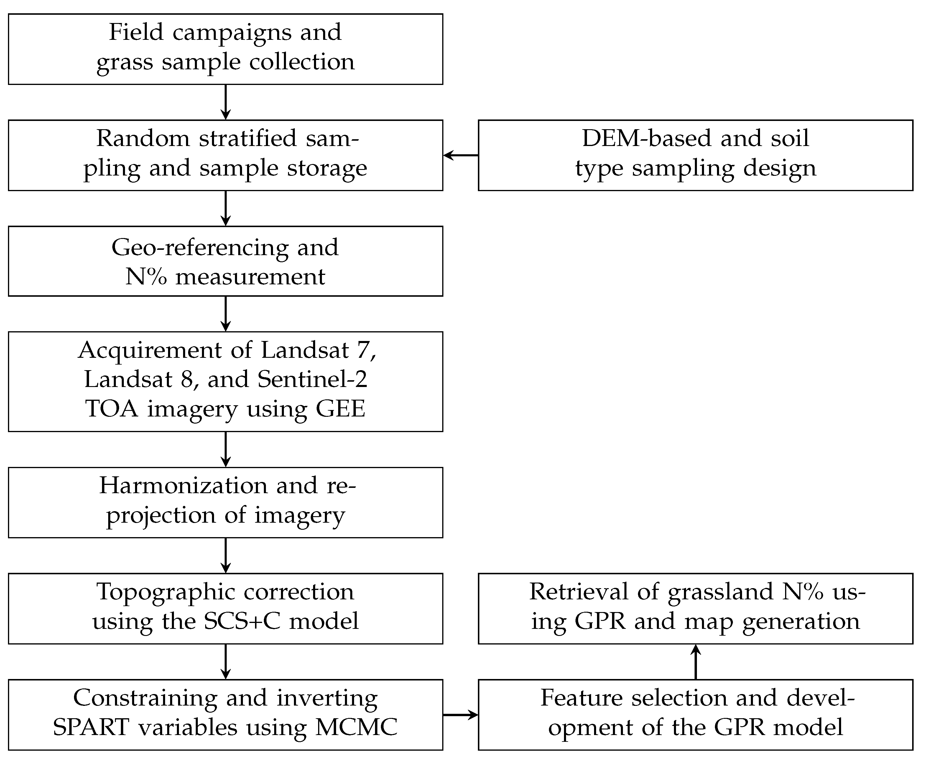
2. Material and Methods

2.1. Field Campaigns and Chemical Analysis

We collected 700 grass samples between 2016 and 2019 from five different hill country and dairy farms across the North and South Islands of New Zealand, ensuring significant variability in our study (Table A1). We employed random stratified sampling based on slope angle, aspect, and soil types. Slope angles were categorized into groups 0–8, 8–16, 16–25, and 25+ degrees. The open-source digital elevation model (DEM) from Land Information in New Zealand (LINZ) was used for our sampling design. At each location, a 0.5 square meter quadrant was placed on the grassland, and the grass was harvested using an electric shearing machine before being stored in a cooling box [58,59,60]. Each site was geo-referenced with an RTK-GPS system, and photographs were taken for visual assessment. Grass samples were sent to Analytical Research Laboratories (ARL) in Napier, New Zealand, for N% measurement using the Kjeldahl method [61]. Samples were dried, ground, and homogenized with a mixer mill [62]. To ensure accurate and reliable measurements, we collected data from grass-covered areas with a leaf area index (LAI) range of one to four. LAI is a dimensionless indicator that quantifies the leaf area per unit of ground area, providing essential information on the vegetation’s structure and density. This LAI range allows for the precise capture of the canopy’s spectral characteristics while minimizing the influence of the surrounding soil background, ensuring proper sensor calibration for vegetation canopy detection and reducing the contribution of soil background to the spectral measurements. By adhering to these sampling guidelines, our data collection was robust and representative of the grassland conditions in the study area. Detailed accounts of our field campaigns and dataset can be found in Dehghan-Shoar et al. [9], Pullanagari et al. [18].

2.2. Spaceborne Optical Imagery Harmonization and Topographical Correction

We identified and downloaded L7, L8, and S2 TOA imagery for dates on which our samples were collected (Table 1). This process was undertaken using the Google Earth Engine (GEE) cloud computing platform and the geo-referenced sampling locations [63]. We used satellite imagery captured within seven days with less than 15 percent cloud coverage. We harmonized the imagery captured by different sensors using BRDF, hence re-projecting the L7, L8, and S2 TOA imagery to Nadir [64]. We utilized the spectrally equivalent MODIS (moderate resolution imaging spectroradiometer) bands L7, L8, and S2, along with the corresponding spectral BRDF model parameters suggested by Roy et al. [28,65]. This method was selected based on its demonstrated high performance and ease of use in calculations when harmonizing both the S2 and L8 TOA data [66].
To ensure that the data from different data sources with varying spectral and radiometric characteristics are comparable and consistent, we implemented the modified sun–canopy–sensor (SCS+C) model for the topographic correction of each image. The SCS+C method enhances the standard sun–canopy–sensor topographic correction by incorporating diffuse atmospheric irradiance [33,40]. To perform topographic correction, we used metadata-based observation and solar angle information, as well as topographic information calculated from the shuttle radar topography mission (SRTM) digital elevation model (DEM), including slope and slope aspect [67]. Additionally, we co-registered the DEM layer and the optical imagery to improve alignment and reduce misregistration errors. Finally, the L7, L8, and S2 TOA reflectance and DEM imagery were spatially resampled to 10-meter (m) spatial resolution using the nearest neighbor algorithm for further analysis.

2.3. RTM Variable Inversion

The spectral signature for each sample was extracted from the pre-processed L7, L8, and S2 imagery. The extracted spectra correspond to values of a single pixel overlapping with the captured GPS locations. Due to the impact of shadow and cloud coverage, some samples were manually removed from the dataset. Using numerical optimization, we used the SPART model with the extracted L7, L8, and S2 TOA data to invert the biochemical and biophysical variables. This model uses a vegetation canopy RTM, commonly referred to as PROSAIL. PROSAIL was developed using the SAIL and PROSPECT models first proposed by Verhoef [10] and Jacquemoud and Baret [41]. In this work, we implemented the latest variation of PROSPECT called PROSPECT-PRO, as it enables the forward and inverse simulation of vegetation protein content [16]. The SPART model also couples the brightness–shape–moisture (BSM) and simplified method for atmospheric correction (SMAC) RTM models; hence, it is capable of simulating the biochemical and biophysical variables of vegetation from TOA data [54,55,68,69].
We used a Markov chain Monte Carlo (MCMC) numerical optimization algorithm with a total sum of error as the loss function to invert each sample’s biophysical and biochemical variables using SPART [70]. We used MCMC, as it can sample from high-dimensional probability distributions associated with RTM problems. In addition, MCMC can calculate the uncertainty associated with each inverted variable. We parametrized the MCMC sampling algorithm using an ensemble sampler with 100 walkers operating for 10,000 simulations per sample. To address the ill-posed nature of RTM, we constrained some of the SPART variables based on prior knowledge and available data, including soil parameters, geographical location, atmospheric parameters, viewing and illumination geometry, and day of year (DOY) required by SPART (Table 2) [50]. We estimated the SPART ozone, aerosol, and water vapor values using the Total Ozone Mapping Spectrometer (TOMS), MODIS/Terra Aerosol Cloud Water Vapor, and the NCEP/NCAR 40-Year Reanalysis Project datasets available from GEE [71,72,73]. After undertaking the simulations using MCMC, we performed thinning to calculate the mean and one-sigma standard deviation for each inverted variable.

2.4. Retrieval of Grassland N%

After retrieving each sample’s biochemical and biophysical variables using the L7, L8, and S2 reflectance, we focused on developing a model to predict grassland N%. We employed a Gaussian process regressor (GPR) algorithm that leverages the inverted biochemical and biophysical variables from TOA imagery for model calibration [74]. GPR is a robust non-parametric method modeling the relationship between input and output variables. It assumes that the function values at any set of input points are jointly Gaussian-distributed, enabling uncertainty estimates for predictions at new, unseen input points [75]. A kernel function, chosen to measure the similarity between input points, is vital for performing GPR. The kernel function influences the model’s behavior and helps learn complex patterns in the data. Various kernel functions exist, including the squared exponential kernel, the Matern kernel, and the radial basis function (RBF) kernel. We optimized our model using the random search optimization (RSO) algorithm, which identified the RBF kernel as the optimal parameter for the GPR [76].
We validated our model using spatially and temporally independent data from L7, L8, and S2 TOA reflectance data to predict grassland N%. The dataset we used in this study consisted of 377 for S2, 277 for L7, and 46 for L8 samples. We used 30% (n = 210) of our total dataset for independent validation, while the remaining samples were used for calibration and cross-validating purposes. Due to the imbalanced nature of our dataset, we used the synthetic minority over-sampling technique for regression with Gaussian noise (SMOGN) on the calibration data. This method performs the synthetic minority over-sampling technique for regression (SMOTER) with traditional interpolation and Gaussian noise (SMOTER-GN) [77]. To achieve the best possible results, we optimized the default parameters for the method, setting the number of neighbors for over-sampling to 6, perturbation or noise percentage to 0.02, and a threshold of 0.5. Furthermore, we identified the most informative biochemical and biophysical variables for predicting grassland N% using the recursive feature elimination algorithm (RFE) and GPR [78,79]. RFE is a commonly used feature selection technique that fits a model and removes the least important variables from a dataset until the existing requirements have been met (specified number of features, in our case, five).
Followed by this procedure, we calculated the mean and standard deviation of the predicted values. These values are then used to measure the performance of our methodology by calculating statistical metrics, including R 2 , root mean squared error (RMSE), and mean prediction interval width (MPIW) [80]. In addition, we investigated the impact of slope angle, slope aspect, viewing, and illumination geometry on the spectra captured by each sensor, by comparing the impact of these variables on the simulated and real harmonized and topographically corrected reflectance. In addition, we investigated the impact of the topographical correction on our model performance using the validation dataset. The flowchart containing the methodology used in this study is illustrated in Figure 1.

3. Results

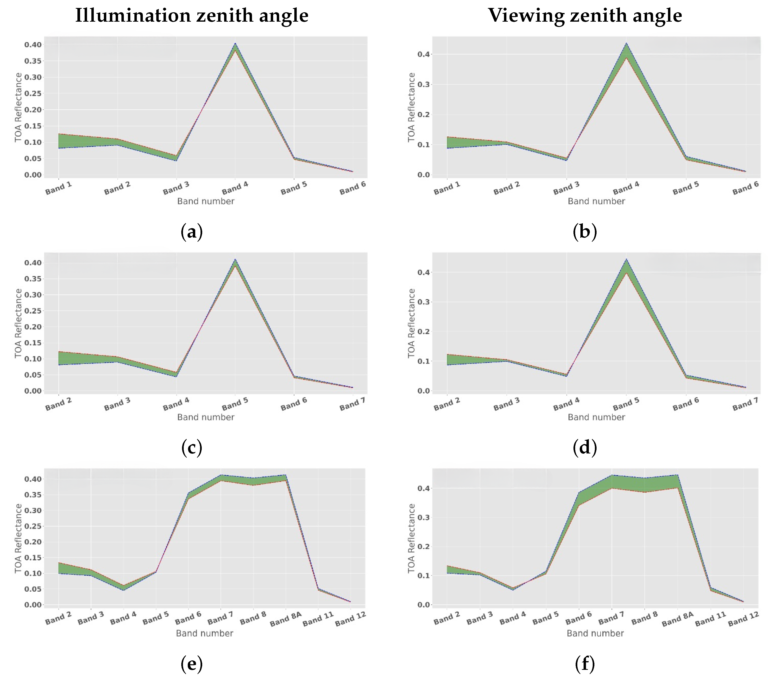
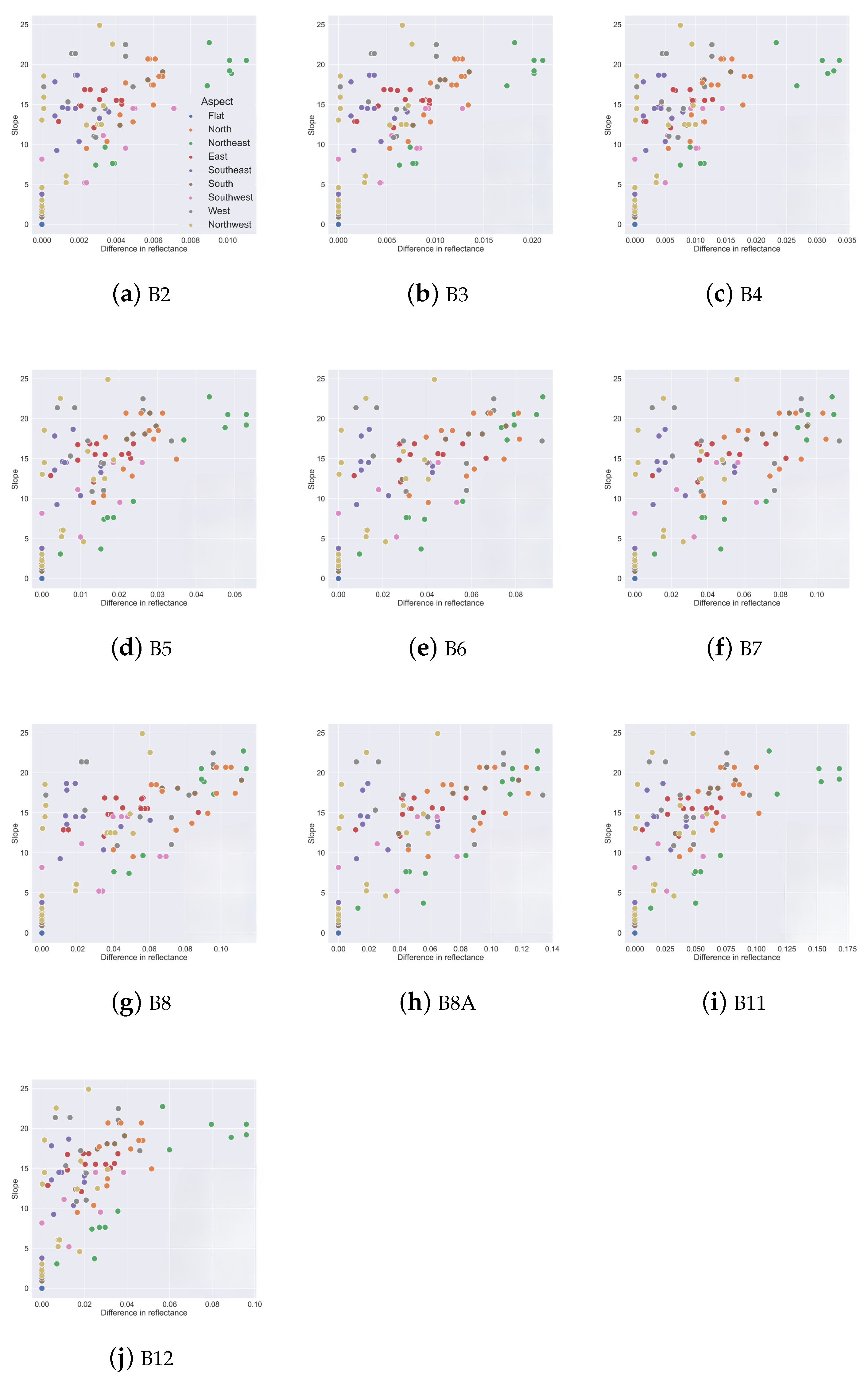
3.1. Impact of Viewing and Illumination Geometry on Simulated TOA Reflectance

By fixing all SPART parameters while changing the viewing and illumination angles of SPART (shaded green area of Figure 2), we estimated the sensitivity of TOA reflectance to viewing geometry. This indicates that the viewing zenith angle impacts the VIS and NIR of TOA reflectance, while the illumination zenith angle has a limited impact. A higher viewing zenith angles result in lower reflectance in the NIR, with a decrease of greater than 10%. Lower illumination zenith angle values increase the TOA reflectance. Similarly, variation of the illumination zenith angle has a limited influence, with a decrease of less than 3%, on other parts of the spectrum, such as the SWIR.
The impact of viewing and illumination geometry on TOA reflectance is noticeably pronounced in rugged terrain, whereas this effect is relatively minimal in flat areas. As illustrated in Figure 3, a considerable visual difference between rugged and flat terrains regarding TOA reflectance highlights the sensitivity of rugged terrain to illumination and viewing geometry. Moreover, the red circles in the same figure further emphasize the limited impact observed in flat regions, which is consistent with the notion that the effect of viewing and illumination geometry on TOA reflectance is generally more pronounced in rugged terrain.

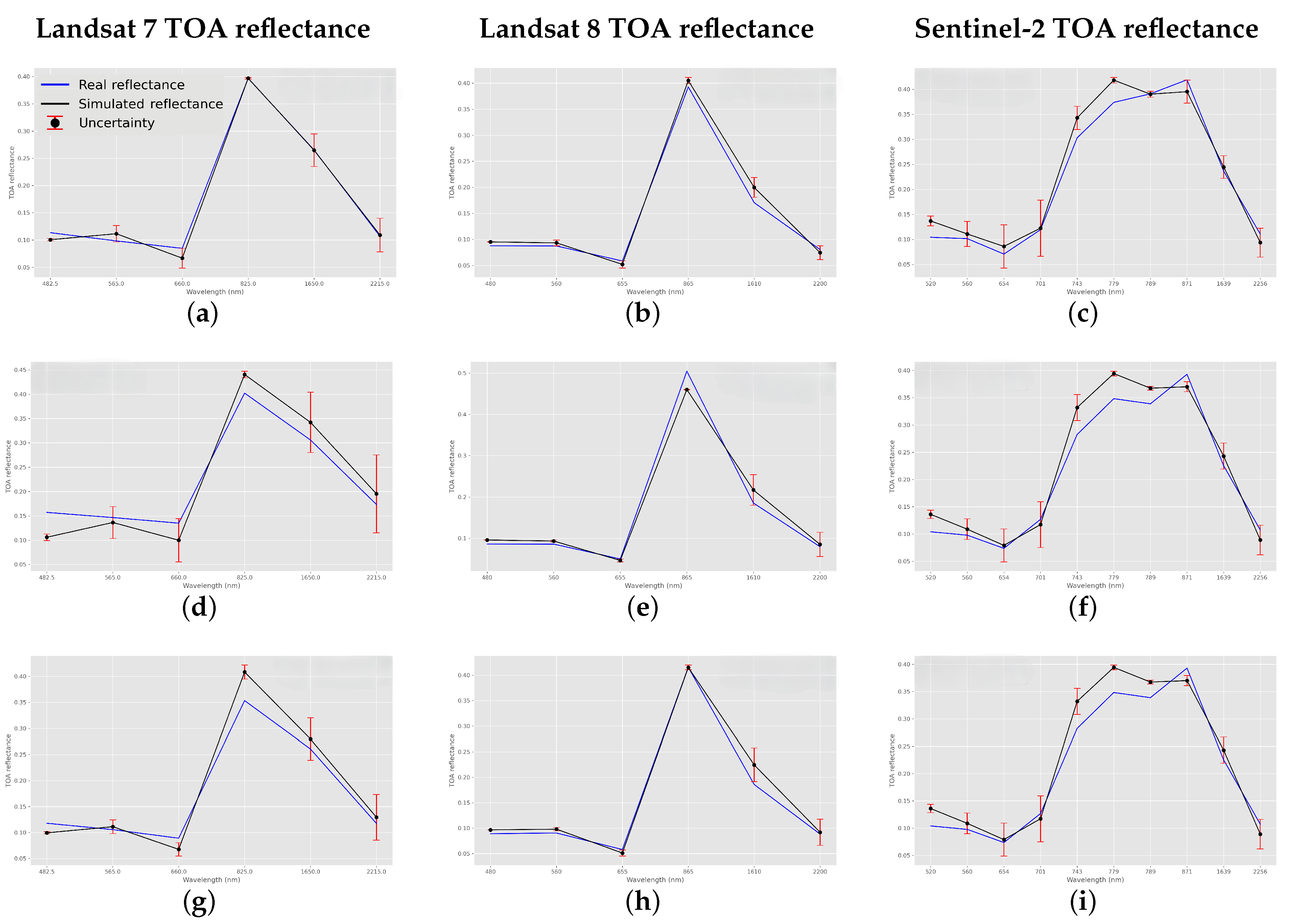
3.2. Inversion of SPART Variables

We used SPART and an MCMC numerical inversion method to simulate spectral data and retrieve the biochemical and biophysical variables. The simulation aimed to minimize the difference between the actual and simulated spectral data as described in [17]. This simulation showed higher uncertainty in the NIR region of the L7, L8, and S2 data sets, as demonstrated in Figure 4.

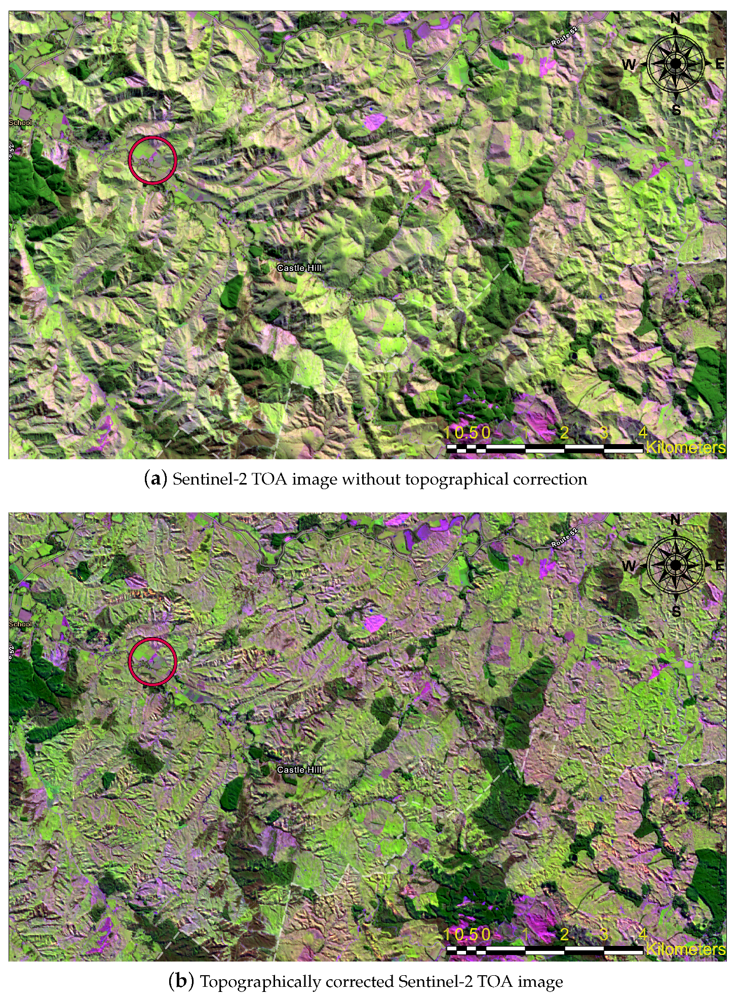
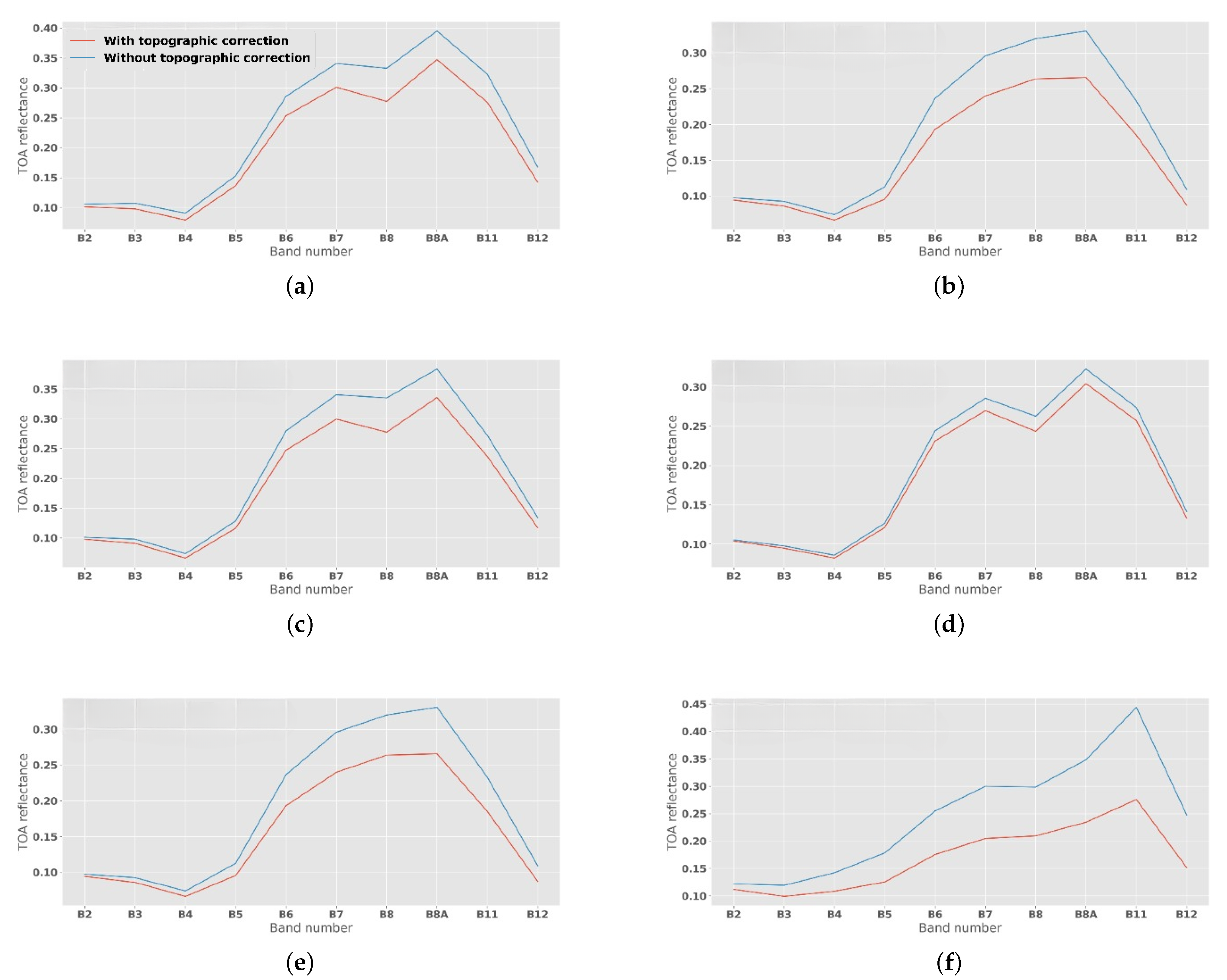
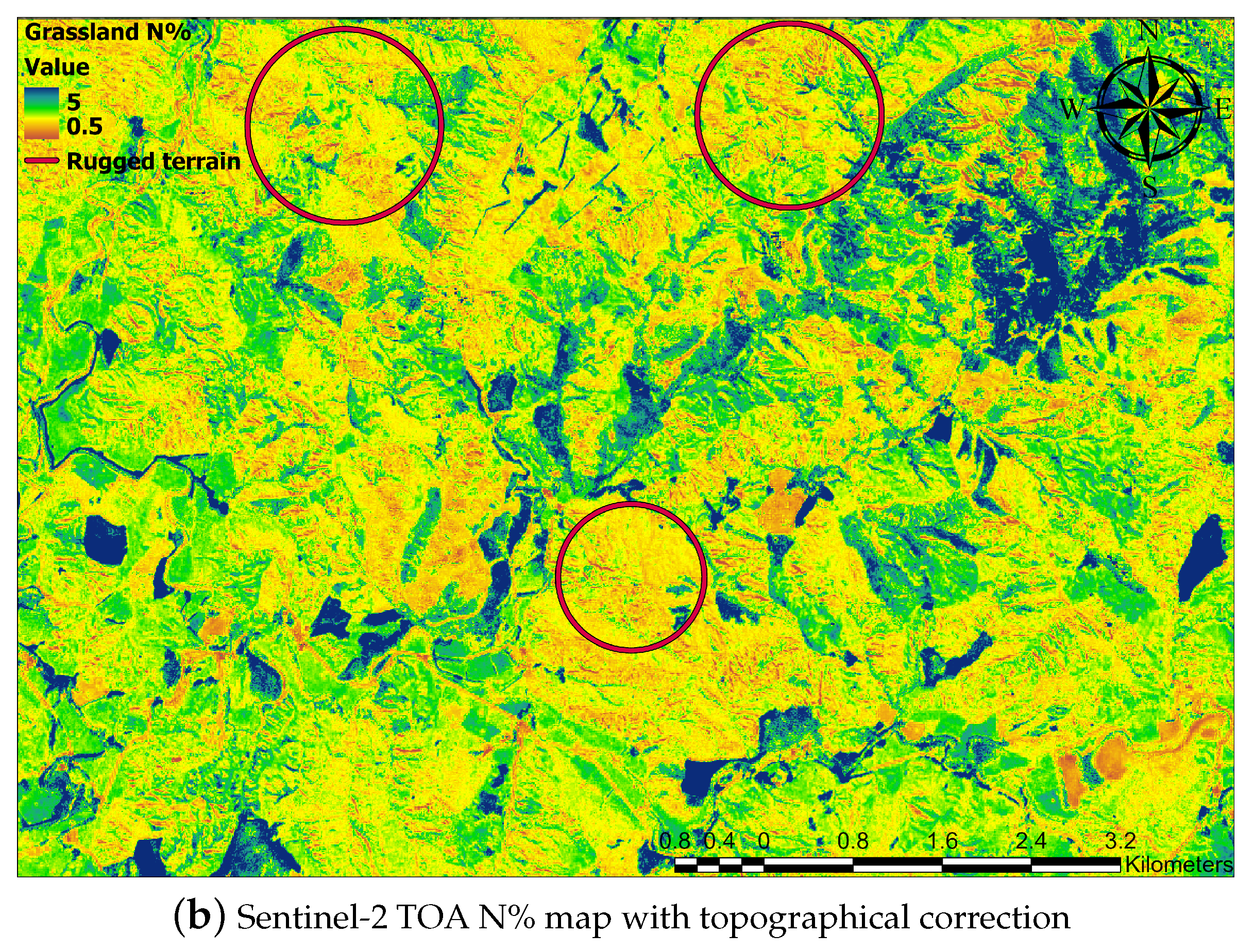
3.3. Impact of Topographic Correction on TOA Reflectance

We applied the SCS+C method for topographic correction after implementing BRDF to harmonize sensor data. Our findings reveal a notable visual contrast in rugged terrain before and after topographic correction. At the same time, minimal differences are observed in flat areas (as emphasized in red in Figure 3). Following topographic correction, the NIR spectral reflectance decreases in rugged terrain, aligning with our observations in Figure 3 and Figure 5. This reduction in NIR spectral reflectance can be due to the variations in surface slope and orientation associated with a rugged terrain. Such variations can influence the amount of sunlight reflected by the surface, and topographic correction compensates for these disparities, yielding a more precise estimate of the surface reflectance.
We investigated the impact of slope angle and slope aspect on each spectral band of S2 TOA reflectance, as illustrated in Figure 6. Our results show that a higher slope value is usually associated with a greater difference (on average, better than 10% in the NIR). In particular, when the aspect is northeast and southwest facing, the difference between the reflectance values is typically higher. This is because the terrain is facing the sun during image acquisition. Furthermore, the NIR (B6, B7 and B8, and B8A) is highly impacted by steep terrain in comparison with the visible region (B2, B3, and B4) and SWIR (B11 and B12).

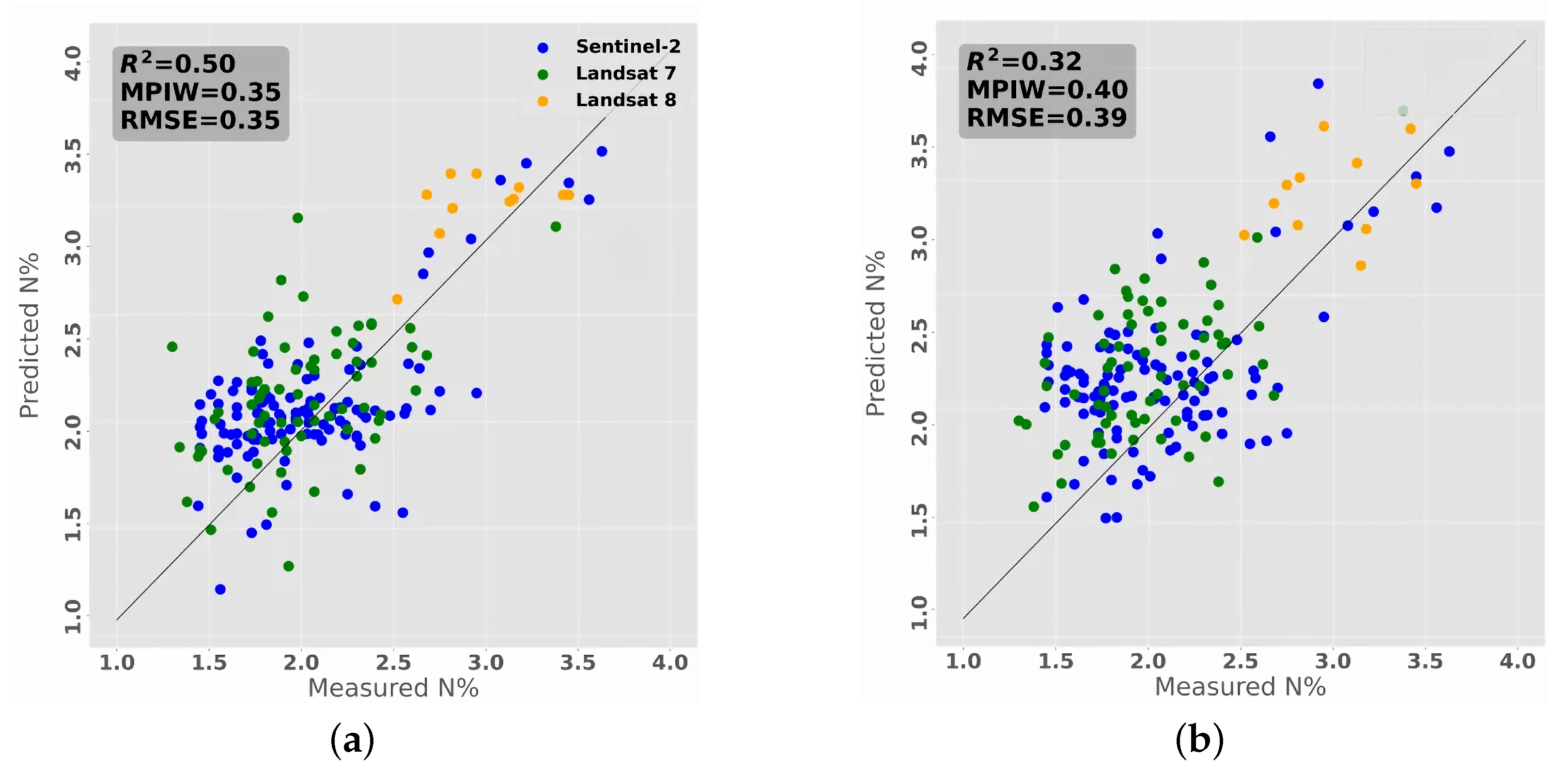
3.4. Validation Results of the Model

Cab, Cw, Cbc, LIDFa, and LAI were identified as the most informative features for predicting N% in vegetation based on the RFE technique. Among these variables, Cab, representing chlorophyll-a concentration, is the most important due to its strong correlation with N%, as both are essential for photosynthesis [17,81]. Cw is related to N% through its role in cellular hydration, while Cbc is indirectly associated with N% through the carbon–nitrogen balance in plants [82]. LIDFa provides insights into canopy structure influenced by nitrogen availability, and LAI indicates vegetation density, which is also affected by nitrogen availability [18]. Using these biochemical and biophysical variables derived from TOA reflectance, we calibrated our model with an optimized GPR algorithm for predicting N% in vegetation.
We evaluated our GPR model’s performance using spatially and temporally independent biochemical and biophysical data from L7, L8, and S2 satellite imagery. Our model demonstrated moderate performance using topographically corrected TOA reflectance data, achieving R 2 values of 0.5, RMSE values of 0.35, and MPIW values of 0.35, as shown in Figure 7a. However, when not using topographically corrected data, the model’s performance declines, resulting in R² values of 0.32, RMSE values of 0.40, and MPIW values of 0.39, as depicted in Figure 7b. The difference in prediction accuracy can be attributed to the importance of accounting for topographic effects on reflectance data, which helps improve the model’s ability to accurately estimate biochemical and biophysical properties. Additionally, combined uncertainties from model inversion, BRDF effects, and topography contribute to the observed discrepancies in model performance, which are also present in N% maps generated (Figure 8). Addressing these sources of uncertainty is essential for enhancing the reliability and accuracy of remote sensing-based models when estimating vegetation properties.

4. Discussion

4.1. Impact of Viewing and Illumination Geometry

Vegetation Cab and Cp are often used as proxies for predicting grassland N% as these two variables are closely linked to vegetation N% [8,83,84]. Since the spectral absorption associated with Cab is present in the VIS of the spectrum, Cab can be used as a robust proxy for monitoring grassland N% without applying BRDF correction. However, despite the promising results achieved for monitoring N using Cab, Cp is the main source of N in vegetation, and the accurate retrieval of Cp is critical for monitoring N% [16]. Key bands for estimating protein are scattered across the electromagnetic spectrum (particularly in the SWIR); as a result, BRDF remains an important step for inverting Cp using RTM. It is important to identify and constrain all sources of uncertainty and error to accurately invert RTM variables using numerical inversion (MCMC) (Figure 4). However, there is uncertainty with inverted variables derived using MCMC uncertainties associated with the NIR and SWIR caused by several factors, including the inversion process of SPART variables. As many factors impact the SWIR (e.g., atmospheric variables and viewing geometry), it is important to identify and isolate different sources of error and uncertainty (including viewing and illumination geometry) for inverting Cp, thus predicting accurate N%. This becomes more critical when developing invariant sensor models due to the differences in the sensor specifications.
Our study aimed to evaluate the impact of viewing and illumination geometry on spectra, particularly in the VIS and NIR regions. The results revealed that geometry significantly affects both regions, consistent with previous research by Mao et al. [85] that reported the sensitivity of the spectral regions between 760 nm to 890 nm and 450 nm to 680 nm with geometric factors. This sensitivity can be attributed to the anisotropy of the vegetative canopy and its interaction with radiation as explained by [86]. Moreover, our study showed that predicted biomass values are more sensitive to geometric factors than biochemical and biophysical variables impacted by the VIS region, consistent with the findings of Buchhorn et al. [87], who investigated the impact of geometry on various variables, including biomass. Ignoring these factors can lead to misleading conclusions, as demonstrated by Mao et al. [85]. Therefore, our results highlight the importance of considering viewing and illumination geometry, particularly in the NIR region, when predicting biomass values. Additionally, neglecting BRDF effects, as highlighted by Buchhorn et al. [87], can result in inaccurate estimations of biochemical and biophysical variables of vegetation.

4.2. Impact of Topography

Topographical correction can significantly impact spectra when the terrain is steep and facing the sun as shown in Figure 6. This is because steep terrain receives more solar irradiance, which affects the measured reflectance [34,88]. Topographical factors significantly impact longer wavelengths (greater than 750 nm), making it difficult to retrieve certain biochemical and biophysical variables, such as LAI, Cw, and Cbc, which have characteristic absorption in these regions. This can lead to inaccurate estimation of N% using SPART. To investigate this issue, we compared the performance of our model with and without topographical correction. Our findings show that topographical correction improves model performance and transferability, particularly in rugged shadow-dominated terrain. de Oliveira et al. [89] investigated the interaction between topographic factors on vegetation indices derived from hyperspectral imagery. They found that most vegetation indices related to biochemical and biophysical variables and plant physiology have some degree of anisotropy with terrain illumination effects, consistent with our findings (Figure 3 and Figure 5). There are significant visual differences before and after topographic correction. This change in reflectance could have a significant impact on the inversion of SPART variables, adding error and uncertainty to our model.
In addition, we observed the “over-correction” of spectra, where the terrain is not facing the sun. The SCS+C proposed by Soenen et al. [40] reduces the over-correction of spectra by introducing the C parameter as an empirical coefficient to calculate diffuse skylight irradiance. Given the simplicity of the SCS+C model and lack of consideration of the anisotropic irradiance and reflectance, this model cannot generalize well to multiscale topographic regions Bishop et al. [88]. Bishop et al. [88] has discovered that it is very challenging to accurately retrieve biophysical variables of a scene by using empirical topographical correction methods. A detailed investigation is required to develop transferable and physically based topographical correction techniques for retrieving grassland spectra in rugged terrain.
A limitation of this work is that the topographical correction procedure used is a low spatial resolution DEM layer. This limitation can lead to errors and uncertainties in the topographically corrected image, impacting the estimation of biophysical and biochemical variables, including LAI and Cab. The implications of inaccurate estimation of these variables can have far-reaching consequences for vegetation monitoring and management (e.g., estimation of N%). Higher-quality data sources, such as light detection and ranging (LiDAR) products, can provide highly accurate and detailed elevation data for topographical correction. This could reduce errors and uncertainties in the corrected image, improving biophysical and biochemical variable estimation accuracy and, therefore, N% retrieval. It is essential to note that using higher-quality data sources, such as LiDAR, can come at a higher cost regarding financial resources and time. Therefore, researchers and practitioners must carefully consider the trade-offs between data quality and cost effectiveness when selecting data sources for topographical correction.

4.3. The Performance of the Model

The proposed model can predict grassland N% using the biochemical and biophysical variables derived from multiple satellite imagery (Figure 7). The independent validation results of our model are promising and show good performance, consistent with results achieved in other work (Figure 4) [17,90]. Furthermore, our results demonstrate that the topographically corrected data perform better in terms of RMSE, MPIW, and R 2 compared to data retrieved without undertaking topographical correction.
Using RFE, we identified Cab, LAI, LIDFa, Cbc, and Cw as the critical variables for predicting N%. The importance of these variables highlights the need for topographical correction and BRDF correction, which can improve the accuracy of the predictions. By inverting the variables and using physical characteristics from the RTM, we can develop transferable models that consider several physical parameters impacting the spectra. This approach allows us to combine physical and empirical information, taking advantage of both methods and improving the robustness of our predictions. The selection of these biophysical and biochemical variables by RFE depicts the importance of above ground biomass (AGB) and chlorophyll for estimating N%. Although there is no direct relationship between N% and AGB, there is an indirect relationship between the two because higher N% positively correlates with AGB for grasslands [91]. Our research found that LAI, Cw, and Cbc are essential for estimating N% proxies for fresh AGB. This aligns with the findings of Wocher et al. [92], which showed that LAI, Cw, Cp, and Cbc could be used to estimate AGB. It is important to note that while models trained using spectra and similar empirical and statistical methods may still provide helpful information, they may not be as transferable as models that combine physical and empirical information. By considering both methods, we aim to improve the accuracy and reliability of our predictions of N%.
Even though Cp is the main N-containing biochemical in grassland, the RFE algorithm has yet to identify this variable as necessary. This is because of the uncertainty and error in the inversion process and limitations of the sensors (e.g., low spectral and spatial resolution and poor signal-to-noise ratio of the SWIR). Alternatively, Cab is selected as an essential variable for estimation N%, as Cab is the second-most N-containing biochemical variable in vegetation [83,84]. The lack of selection of Cp for predicting N% highlights the importance of identifying and addressing different sources of error and uncertainty, including topography and geometry, when monitoring grassland N% in rugged terrain.

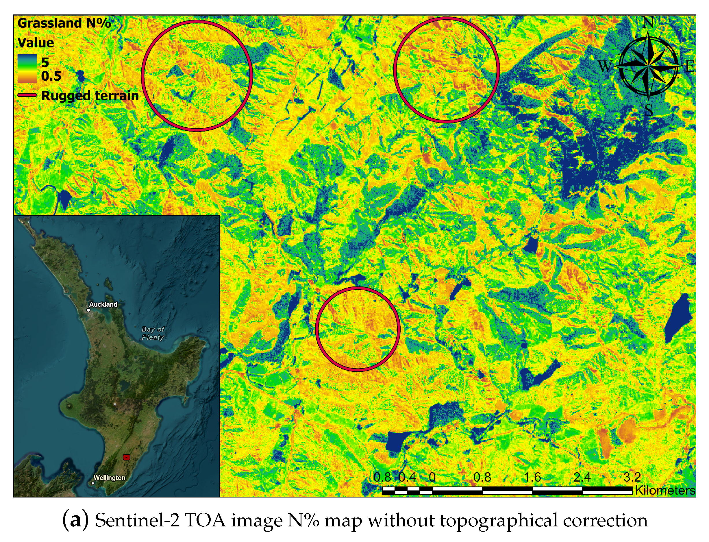
4.4. Enhancing RTM for Monitoring Grassland N% in Rugged Terrain

Enhancing the accuracy of the proposed model for grassland N% prediction requires addressing factors that affect input variable quality and inversion process precision. This can be achieved using higher spectral resolution instruments, such as hyperspectral imagery with a superior signal-to-noise ratio (SNR), to collect high-quality spectral data and enable a more precise inversion process [9]. Improvements to the model’s accuracy can also result from refining the statistical and physically based models used in the inversion process, such as algorithm advancements, data incorporation, or parameter adjustments [93,94]. Moreover, exploring new methods for obtaining RTM variables and enhancing the inversion process may be beneficial. Addressing these factors can improve model accuracy and provide reliable grassland N% monitoring results.
This study demonstrated promising results in monitoring grassland N% using BRDF and topographical correction techniques. Although our approach offers higher temporal resolution through various optical spaceborne instruments, periods with limited optical imagery remain. Therefore, exploring alternative methods for improving temporal resolution in N% monitoring is essential. Further enhancements are required to monitor grassland biophysical and biochemical variables. Our results suggest that integrating BRDF and topographical correction techniques has the potential for grassland N% monitoring. However, limitations exist, including limited temporal resolution and the need to refine statistical and physically based models within the inversion process. Future research could explore physics-informed machine learning algorithms for vegetation N% monitoring, given the strong correlation between N% Cab and Cp [95,96]. Implementing such strategies may enable more accurate and reliable monitoring across different vegetation species.

5. Conclusion

Our study presents a novel physically based sensor workflow for monitoring grassland N% using spaceborne optical imaging. Our approach integrates multiple RTMs with L7, L8, and S2 TOA reflectance data, BRDF for sensor harmonization, and SCS+C for topographical correction. The key findings of our work are as follows:
  • Our approach achieves an independent validation accuracy of 0.35 (RMSE %N), a mean prediction interval width value of 0.35, and an R 2 of 0.50 using independent validation data from multiple sensors between 2016 and 2019, demonstrating the potential for the cost-efficient monitoring of grassland N% using various spaceborne optical instruments in rugged terrain.
  • We investigated the impact of rugged terrain, viewing, and illumination on different sensors’ spectral reflectance for estimating grassland N%, showing that viewing and illumination geometry can significantly impact spectra, particularly in longer wavelengths. Moreover, topographic correction is essential for monitoring grassland characteristics in rugged terrain.
  • To address the ill-posed nature of RTM, it is essential to identify and address sources of uncertainty, including topography and viewing and illumination geometry. Future research should investigate the impact of different BRDF and topographical correction methods on retrieving grassland N%.
  • Although our proposed methodology provides higher temporal resolution for monitoring grassland N%, there are still periods where acquiring optical imagery is challenging. Therefore, it is crucial to investigate alternative methods of continuously monitoring grassland characteristics.
  • Further investigation should be undertaken using physically guided machine learning algorithms to monitor N%. This will enable the development of high-performance sensor models for monitoring vegetation characteristics across different species.
Overall, our study represents a significant step forward in developing an efficient approach for monitoring grassland N%, with important implications for improving the sustainability of agriculture and the environment. Our approach offers a low-cost and continuous monitoring solution for grassland N% that reduces the negative impact of chemical nitrogen fertilizers on the environment. Additionally, our approach is available on cloud services, providing increased accessibility for users.

Author Contributions

Conceptualization, M.H.D.-S. and A.A.O.; Methodology, M.H.D.-S. and R.R.P.; Software, M.H.D.-S.; Validation, M.H.D.-S.; Formal analysis, M.H.D.-S. and A.A.O.; Investigation, M.H.D.-S. and G.K.; Resources, R.R.P.; Writing – original draft, M.H.D.-S., R.R.P., G.K., A.A.O., I.J.Y., and J.H.; Writing – review & editing, M.H.D.-S., R.R.P., G.K., A.A.O., I.J.Y., and J.H.; Visualization, M.H.D.-S.; Supervision, R.R.P., G.K., A.A.O., I.J.Y., and J.H.; Project administration, I.J.Y.; Funding acquisition, R.R.P. and I.J.Y. All authors have read and agreed to the published version of the manuscript.

Funding

This research received no external funding.

Data Availability Statement

The data that has been used is confidential.

Acknowledgments

This work has been supported by Pastoral 21 research programme, The C. Alma Baker Trust, Ministry for Primary Industries and Ravensdown, New Zealand. Furthermore, we would like to acknowledge the contribution of staff and students of Massey University and staff of AgResearch New Zealand for collecting the field samples.

Conflicts of Interest

The authors declare no conflict of interest.

Appendix A

Table A1. Table containing the ID list of the acquired L7, L8 and S2 TOA imagery. The imagery was acquired when the cloud coverage was less than 15 percent.
InstrumentImage ID
Sentinel-2COPERNICUS/S2/20160426T221552_20160426T221553_T60GUA
Sentinel-2COPERNICUS/S2/20190330T222539_20190330T222539_T59GNM
Landsat 8LANDSAT/LC08/C01/T1_TOA/LC08_073087_20181018
Landsat 7LANDSAT/LE07/C01/T1_TOA/LE07_07208_20160420
Landsat 7LANDSAT/LE07/C01/T1_TOA/LE07_072088_20191123

References

  1. Steinfeld, H.; Gerber, P.; Wassenaar, T.D.; Castel, V.; Rosales, M.; Rosales, M.; de Haan, C. Livestock’s Long Shadow: Environmental Issues and Options; Food & Agriculture Organization: Roma, Italy, 2006. [Google Scholar]
  2. Rouse, J.D.; Bishop, C.A.; Struger, J. Nitrogen pollution: An assessment of its threat to amphibian survival. Environ. Health Perspect. 1999, 107, 799–803. [Google Scholar] [CrossRef] [PubMed]
  3. Bassi, D.; Menossi, M.; Mattiello, L. Nitrogen supply influences photosynthesis establishment along the sugarcane leaf. Sci. Rep. 2018, 8, 2327. [Google Scholar] [CrossRef] [PubMed]
  4. Howarth, R.W. Coastal nitrogen pollution: A review of sources and trends globally and regionally. Harmful Algae 2008, 8, 14–20. [Google Scholar] [CrossRef]
  5. Pullanagari, R.; Kereszturi, G.; Yule, I. Mapping of macro and micro nutrients of mixed pastures using airborne AisaFENIX hyperspectral imagery. ISPRS J. Photogramm. Remote Sens. 2016, 117, 1–10. [Google Scholar] [CrossRef]
  6. Frampton, W.J.; Dash, J.; Watmough, G.; Milton, E.J. Evaluating the capabilities of Sentinel-2 for quantitative estimation of biophysical variables in vegetation. ISPRS J. Photogramm. Remote Sens. 2013, 82, 83–92. [Google Scholar] [CrossRef]
  7. Szantoi, Z.; Strobl, P. Copernicus Sentinel-2 calibration and validation. Eur. J. Remote Sens. 2019, 52, 253–255. [Google Scholar] [CrossRef]
  8. Berger, K.; Verrelst, J.; Féret, J.B.; Hank, T.; Wocher, M.; Mauser, W.; Camps-Valls, G. Retrieval of aboveground crop nitrogen content with a hybrid machine learning method. Int. J. Appl. Earth Obs. Geoinf. 2020, 92, 102174. [Google Scholar] [CrossRef]
  9. Dehghan-Shoar, M.H.; Orsi, A.A.; Pullanagari, R.R.; Yule, I.J. A hybrid model to predict nitrogen concentration in heterogeneous grassland using field spectroscopy. Remote Sens. Environ. 2023, 285, 113385. [Google Scholar] [CrossRef]
  10. Verhoef, W. Light scattering by leaf layers with application to canopy reflectance modeling: The SAIL model. Remote Sens. Environ. 1984, 16, 125–141. [Google Scholar] [CrossRef]
  11. Verhoef, W. Theory of radiative Transfer Models Applied in Optical Remote Sensing of Vegetation Canopies; Wageningen University and Research: Wageningen, The Netherlands, 1998. [Google Scholar]
  12. Estévez, J.; Vicent, J.; Rivera-Caicedo, J.P.; Morcillo-Pallarés, P.; Vuolo, F.; Sabater, N.; Camps-Valls, G.; Moreno, J.; Verrelst, J. Gaussian processes retrieval of LAI from Sentinel-2 top-of-atmosphere radiance data. ISPRS J. Photogramm. Remote Sens. 2020, 167, 289–304. [Google Scholar] [CrossRef]
  13. Richter, R.; Schläpfer, D. Atmospheric/topographic correction for airborne imagery. In ATCOR-4 User Guide; ReSe Applications Schläpfer, D., Ed.; IMAGINE Photogrammetry, Remote Sensing, and GIS Software: Graz, Austria, 2011; pp. 565–602. [Google Scholar]
  14. Richter, R.; Schläpfer, D. Atmospheric/topographic correction for satellite imagery. In DLR Report DLR-IB; German Aerospace Center (DLR): Berlin, Germany, 2005; Volume 565. [Google Scholar]
  15. Curran, P.J. Remote sensing of foliar chemistry. Remote Sens. Environ. 1989, 30, 271–278. [Google Scholar] [CrossRef]
  16. Féret, J.B.; Berger, K.; de Boissieu, F.; Malenovskỳ, Z. PROSPECT-PRO for estimating content of nitrogen-containing leaf proteins and other carbon-based constituents. Remote Sens. Environ. 2021, 252, 112173. [Google Scholar] [CrossRef]
  17. Dehghan-Shoar, M.H.; Pullanagari, R.R.; Orsi, A.A.; Yule, I.J. Simulating spaceborne imaging to retrieve grassland nitrogen concentration. Remote Sens. Appl. Soc. Environ. 2022, 29, 100912. [Google Scholar] [CrossRef]
  18. Pullanagari, R.; Dehghan-Shoar, M.; Yule, I.J.; Bhatia, N. Field spectroscopy of canopy nitrogen concentration in temperate grasslands using a convolutional neural network. Remote Sens. Environ. 2021, 257, 112353. [Google Scholar] [CrossRef]
  19. Fernández-Habas, J.; Moreno, A.M.G.; Hidalgo-Fernández, M.T.; Leal-Murillo, J.R.; Oar, B.A.; Gómez-Giráldez, P.J.; González-Dugo, M.P.; Fernández-Rebollo, P. Investigating the potential of Sentinel-2 configuration to predict the quality of Mediterranean permanent grasslands in open woodlands. Sci. Total Environ. 2021, 791, 148101. [Google Scholar] [CrossRef] [PubMed]
  20. Main-Knorn, M.; Pflug, B.; Louis, J.; Debaecker, V.; Müller-Wilm, U.; Gascon, F. Sen2Cor for sentinel-2. In Proceedings of the Image and Signal Processing for Remote Sensing XXIII, SPIE, Warsaw, Poland, 11–14 September 2017; Volume 10427, pp. 37–48. [Google Scholar]
  21. Goward, S.N.; Masek, J.G.; Williams, D.L.; Irons, J.R.; Thompson, R. The Landsat 7 mission: Terrestrial research and applications for the 21st century. Remote Sens. Environ. 2001, 78, 3–12. [Google Scholar] [CrossRef]
  22. Roy, D.P.; Wulder, M.A.; Loveland, T.R.; Woodcock, C.E.; Allen, R.G.; Anderson, M.C.; Helder, D.; Irons, J.R.; Johnson, D.M.; Kennedy, R.; et al. Landsat-8: Science and product vision for terrestrial global change research. Remote Sens. Environ. 2014, 145, 154–172. [Google Scholar] [CrossRef]
  23. Useya, J.; Chen, S. Comparative performance evaluation of pixel-level and decision-level data fusion of Landsat 8 OLI, Landsat 7 ETM+ and Sentinel-2 MSI for crop ensemble classification. IEEE J. Sel. Top. Appl. Earth Obs. Remote Sens. 2018, 11, 4441–4451. [Google Scholar] [CrossRef]
  24. Shao, Z.; Cai, J.; Fu, P.; Hu, L.; Liu, T. Deep learning-based fusion of Landsat-8 and Sentinel-2 images for a harmonized surface reflectance product. Remote Sens. Environ. 2019, 235, 111425. [Google Scholar] [CrossRef]
  25. Nguyen, M.D.; Baez-Villanueva, O.M.; Bui, D.D.; Nguyen, P.T.; Ribbe, L. Harmonization of landsat and sentinel 2 for crop monitoring in drought prone areas: Case studies of Ninh Thuan (Vietnam) and Bekaa (Lebanon). Remote Sens. 2020, 12, 281. [Google Scholar] [CrossRef]
  26. Claverie, M.; Ju, J.; Masek, J.G.; Dungan, J.L.; Vermote, E.F.; Roger, J.C.; Skakun, S.V.; Justice, C. The Harmonized Landsat and Sentinel-2 surface reflectance data set. Remote Sens. Environ. 2018, 219, 145–161. [Google Scholar] [CrossRef]
  27. Lucht, W.; Schaaf, C.B.; Strahler, A.H. An algorithm for the retrieval of albedo from space using semiempirical BRDF models. IEEE Trans. Geosci. Remote Sens. 2000, 38, 977–998. [Google Scholar] [CrossRef]
  28. Roy, D.P.; Zhang, H.; Ju, J.; Gomez-Dans, J.L.; Lewis, P.E.; Schaaf, C.; Sun, Q.; Li, J.; Huang, H.; Kovalskyy, V. A general method to normalize Landsat reflectance data to nadir BRDF adjusted reflectance. Remote Sens. Environ. 2016, 176, 255–271. [Google Scholar] [CrossRef]
  29. Queally, N.; Ye, Z.; Zheng, T.; Chlus, A.; Schneider, F.; Pavlick, R.P.; Townsend, P.A. FlexBRDF: A flexible BRDF correction for grouped processing of airborne imaging spectroscopy flightlines. J. Geophys. Res. Biogeosci. 2022, 127, e2021JG006622. [Google Scholar] [CrossRef] [PubMed]
  30. Liang, S. Quantitative Remote Sensing of Land Surfaces; John Wiley & Sons: Hoboken, NJ, USA, 2005. [Google Scholar]
  31. Dymond, J.; Shepherd, J.; Qi, J. A simple physical model of vegetation reflectance for standardising optical satellite imagery. Remote Sens. Environ. 2001, 75, 350–359. [Google Scholar] [CrossRef]
  32. Gu, D.; Gillespie, A. Topographic normalization of Landsat TM images of forest based on subpixel sun–canopy–sensor geometry. Remote Sens. Environ. 1998, 64, 166–175. [Google Scholar] [CrossRef]
  33. Chi, H.; Yan, K.; Yang, K.; Du, S.; Li, H.; Qi, J.; Zhou, W. Evaluation of Topographic Correction Models Based on 3-D Radiative Transfer Simulation. IEEE Geosci. Remote Sens. Lett. 2021, 19, 1–5. [Google Scholar] [CrossRef]
  34. Iqbal, M. An Introduction to Solar Radiation; Elsevier: Amsterdam, The Netherlands, 2012. [Google Scholar]
  35. Ono, A.; Kajiwara, K.; Honda, Y.; Ono, A. Development of vegetation index using radiant spectra normalized by their arithmetic mean. In Proceedings of the 42nd Conference of the Remote Sensing Society of Japan, Tokyo, Japan, 9–14 September 2007. [Google Scholar]
  36. Colby, J.D. Topographic normalization in rugged terrain. Photogramm. Eng. Remote Sens. 1991, 57, 531–537. [Google Scholar]
  37. Dozier, J.; Frew, J. Atmospheric corrections to satellite radiometric data over rugged terrain. Remote Sens. Environ. 1981, 11, 191–205. [Google Scholar] [CrossRef]
  38. Richter, R. Correction of atmospheric and topographic effects for high spatial resolution satellite imagery. Int. J. Remote Sens. 1997, 18, 1099–1111. [Google Scholar] [CrossRef]
  39. Teillet, P.; Guindon, B.; Goodenough, D. On the slope-aspect correction of multispectral scanner data. Can. J. Remote Sens. 1982, 8, 84–106. [Google Scholar] [CrossRef]
  40. Soenen, S.A.; Peddle, D.R.; Coburn, C.A. SCS+ C: A modified sun-canopy-sensor topographic correction in forested terrain. IEEE Trans. Geosci. Remote Sens. 2005, 43, 2148–2159. [Google Scholar] [CrossRef]
  41. Jacquemoud, S.; Baret, F. PROSPECT: A model of leaf optical properties spectra. Remote Sens. Environ. 1990, 34, 75–91. [Google Scholar] [CrossRef]
  42. Atzberger, C.; Darvishzadeh, R.; Schlerf, M.; Le Maire, G. Suitability and adaptation of PROSAIL radiative transfer model for hyperspectral grassland studies. Remote Sens. Lett. 2013, 4, 55–64. [Google Scholar] [CrossRef]
  43. Gastellu-Etchegorry, J.; Martin, E.; Gascon, F. DART: A 3D model for simulating satellite images and studying surface radiation budget. Int. J. Remote Sens. 2004, 25, 73–96. [Google Scholar] [CrossRef]
  44. Estévez, J.; Berger, K.; Vicent, J.; Rivera-Caicedo, J.P.; Wocher, M.; Verrelst, J. Top-of-atmosphere retrieval of multiple crop traits using variational heteroscedastic Gaussian processes within a hybrid workflow. Remote Sens. 2021, 13, 1589. [Google Scholar] [CrossRef] [PubMed]
  45. Pu, J.; Yan, K.; Zhou, G.; Lei, Y.; Zhu, Y.; Guo, D.; Li, H.; Xu, L.; Knyazikhin, Y.; Myneni, R.B. Evaluation of the MODIS LAI/FPAR algorithm based on 3D-RTM simulations: A case study of grassland. Remote Sens. 2020, 12, 3391. [Google Scholar] [CrossRef]
  46. Vohland, M.; Mader, S. Numerical minimisation and artificial neural networks: Two different approaches to retrieve parameters from a canopy reflectance model. In Proceedings of the 5th EARSeL Workshop on Imaging Spectroscopy, Bruges, Belgium, 23–25 April 2007; Volume 1. [Google Scholar]
  47. De Wit, A.J. Application of a genetic algorithm for crop model steering using NOAA-AVHRR data. In Proceedings of the Remote Sensing for Earth Science, Ocean, and Sea Ice Applications, SPIE, Florence, Italy, 13–15 December 1999; Volume 3868, pp. 167–181. [Google Scholar]
  48. Lavergne, T.; Kaminski, T.; Pinty, B.; Taberner, M.; Gobron, N.; Verstraete, M.M.; Vossbeck, M.; Widlowski, J.L.; Giering, R. Application to MISR land products of an RPV model inversion package using adjoint and Hessian codes. Remote Sens. Environ. 2007, 107, 362–375. [Google Scholar] [CrossRef]
  49. Berk, A.; Anderson, G.P.; Acharya, P.K.; Bernstein, L.S.; Muratov, L.; Lee, J.; Fox, M.; Adler-Golden, S.M.; Chetwynd, J.H., Jr.; Hoke, M.L.; et al. MODTRAN5: 2006 update. In Proceedings of the Algorithms and Technologies for Multispectral, Hyperspectral, and Ultraspectral Imagery XII Conference, SPIE, Orlando, FL, USA, 17–21 April 2006; Volume 6233, pp. 508–515. [Google Scholar]
  50. Atzberger, C.; Richter, K. Spatially constrained inversion of radiative transfer models for improved LAI mapping from future Sentinel-2 imagery. Remote Sens. Environ. 2012, 120, 208–218. [Google Scholar] [CrossRef]
  51. Sun, J.; Wang, L.; Shi, S.; Li, Z.; Yang, J.; Gong, W.; Wang, S.; Tagesson, T. Leaf pigment retrieval using the PROSAIL model: Influence of uncertainty in prior canopy-structure information. Crop J. 2022, 10, 1251–1263. [Google Scholar] [CrossRef]
  52. Li, H.; Liu, G.; Liu, Q.; Chen, Z.; Huang, C. Retrieval of winter wheat leaf area index from Chinese GF-1 satellite data using the PROSAIL model. Sensors 2018, 18, 1120. [Google Scholar] [CrossRef] [PubMed]
  53. Li, F.; Jupp, D.L.; Thankappan, M.; Lymburner, L.; Mueller, N.; Lewis, A.; Held, A. A physics-based atmospheric and BRDF correction for Landsat data over mountainous terrain. Remote Sens. Environ. 2012, 124, 756–770. [Google Scholar] [CrossRef]
  54. Yang, P.; Verhoef, W.; Van der Tol, C. Unified four-stream radiative transfer theory in the optical-thermal domain with consideration of fluorescence for multi-layer vegetation canopies. Remote Sens. 2020, 12, 3914. [Google Scholar] [CrossRef]
  55. Yang, P.; van der Tol, C.; Yin, T.; Verhoef, W. The SPART model: A soil-plant-atmosphere radiative transfer model for satellite measurements in the solar spectrum. Remote Sens. Environ. 2020, 247, 111870. [Google Scholar] [CrossRef]
  56. Roy, D.P.; Kovalskyy, V.; Zhang, H.; Vermote, E.F.; Yan, L.; Kumar, S.; Egorov, A. Characterization of Landsat-7 to Landsat-8 reflective wavelength and normalized difference vegetation index continuity. Remote Sens. Environ. 2016, 185, 57–70. [Google Scholar] [CrossRef] [PubMed]
  57. D’Odorico, P.; Gonsamo, A.; Damm, A.; Schaepman, M.E. Experimental evaluation of Sentinel-2 spectral response functions for NDVI time-series continuity. IEEE Trans. Geosci. Remote Sens. 2013, 51, 1336–1348. [Google Scholar] [CrossRef]
  58. Hutchinson, K.; Scobie, D.; Beautrais, J.; Mackay, A.; Rennie, G.; Moss, R.; Dynes, R. A protocol for sampling pastures in hill country. J. N. Z. Grasslands 2016, 78, 203–209. [Google Scholar] [CrossRef]
  59. Cosgrove, G.; Betteridge, K.; Thomas, V.; Corson, D. A sampling strategy for estimating dairy pasture quality. In Proceedings of the New Zealand Society of Animal Production Conference, Dunedin, New Zealand, 28–31 July 1998; Volume 58, pp. 25–28. [Google Scholar]
  60. Pullanagari, R.; Yule, I.; Tuohy, M.; Hedley, M.; Dynes, R.; King, W. In-field hyperspectral proximal sensing for estimating quality parameters of mixed pasture. Precis. Agric. 2012, 13, 351–369. [Google Scholar] [CrossRef]
  61. Lynch, J.M.; Barbano, D.M. Kjeldahl nitrogen analysis as a reference method for protein determination in dairy products. J. AOAC Int. 1999, 82, 1389–1398. [Google Scholar] [CrossRef]
  62. Frommer, J.; Voegelin, A.; Dittmar, J.; Marcus, M.A.; Kretzschmar, R. Biogeochemical processes and arsenic enrichment around rice roots in paddy soil: Results from micro-focused X-ray spectroscopy. Eur. J. Soil Sci. 2011, 62, 305–317. [Google Scholar] [CrossRef]
  63. Gorelick, N.; Hancher, M.; Dixon, M.; Ilyushchenko, S.; Thau, D.; Moore, R. Google Earth Engine: Planetary-scale geospatial analysis for everyone. Remote Sens. Environ. 2017, 202, 18–27. [Google Scholar] [CrossRef]
  64. Schaaf, C.B.; Gao, F.; Strahler, A.H.; Lucht, W.; Li, X.; Tsang, T.; Strugnell, N.C.; Zhang, X.; Jin, Y.; Muller, J.P.; et al. First operational BRDF, albedo nadir reflectance products from MODIS. Remote Sens. Environ. 2002, 83, 135–148. [Google Scholar] [CrossRef]
  65. Roy, D.P.; Li, Z.; Zhang, H.K. Adjustment of Sentinel-2 multi-spectral instrument (MSI) Red-Edge band reflectance to Nadir BRDF adjusted reflectance (NBAR) and quantification of red-edge band BRDF effects. Remote Sens. 2017, 9, 1325. [Google Scholar] [CrossRef]
  66. Zhang, H.K.; Roy, D.P.; Yan, L.; Li, Z.; Huang, H.; Vermote, E.; Skakun, S.; Roger, J.C. Characterization of Sentinel-2A and Landsat-8 top of atmosphere, surface, and nadir BRDF adjusted reflectance and NDVI differences. Remote Sens. Environ. 2018, 215, 482–494. [Google Scholar] [CrossRef]
  67. Van Zyl, J.J. The Shuttle Radar Topography Mission (SRTM): A breakthrough in remote sensing of topography. Acta Astronaut. 2001, 48, 559–565. [Google Scholar] [CrossRef]
  68. Verhoef, W.; Van Der Tol, C.; Middleton, E.M. Hyperspectral radiative transfer modeling to explore the combined retrieval of biophysical parameters and canopy fluorescence from FLEX–Sentinel-3 tandem mission multi-sensor data. Remote Sens. Environ. 2018, 204, 942–963. [Google Scholar] [CrossRef]
  69. Rahman, H.; Dedieu, G. SMAC: A simplified method for the atmospheric correction of satellite measurements in the solar spectrum. Remote Sens. 1994, 15, 123–143. [Google Scholar] [CrossRef]
  70. Foreman-Mackey, D.; Farr, W.M.; Sinha, M.; Archibald, A.M.; Hogg, D.W.; Sanders, J.S.; Zuntz, J.; Williams, P.K.; Nelson, A.R.; de Val-Borro, M.; et al. emcee v3: A Python ensemble sampling toolkit for affine-invariant MCMC. arXiv 2019, arXiv:1911.07688. [Google Scholar] [CrossRef]
  71. Parsons, M.A.; Duerr, R.; Minster, J.B. Data citation and peer review. Eos Trans. Am. Geophys. Union 2010, 91, 297–298. [Google Scholar] [CrossRef]
  72. Kalnay, E.; Kanamitsu, M.; Kistler, R.; Collins, W.; Deaven, D.; Gandin, L.; Iredell, M.; Saha, S.; White, G.; Woollen, J.; et al. The NCEP/NCAR 40-year reanalysis project. Bull. Am. Meteorol. Soc. 1996, 77, 437–472. [Google Scholar] [CrossRef]
  73. Hubanks, P.A.; King, M.D.; Platnick, S.; Pincus, R. MODIS atmosphere L3 gridded product algorithm theoretical basis document. In ATBD Reference Number: ATBD-MOD; NASA Goddard Space Flight Center: Greenbelt, MD, USA, 2008; Volume 30, p. 96. [Google Scholar]
  74. Vovk, V. Kernel ridge regression. In Empirical Inference; Springer: Berlin/Heidelberg, Germany, 2013; pp. 105–116. [Google Scholar]
  75. GPy. GPy: A Gaussian Process Framework in Python. 2012. Available online: http://github.com/SheffieldML/GPy (accessed on 5 May 2023).
  76. Bergstra, J.; Bengio, Y. Random search for hyper-parameter optimization. J. Mach. Learn. Res. 2012, 13, 281–305. [Google Scholar]
  77. Branco, P.; Torgo, L.; Ribeiro, R.P. SMOGN: A pre-processing approach for imbalanced regression. In Proceedings of the First International Workshop on Learning with Imbalanced Domains: Theory and Applications, Larnaca, Cyprus, 13 September 2017; PMLR: Exeter, UK; pp. 36–50. [Google Scholar]
  78. Pullanagari, R.R.; Kereszturi, G.; Yule, I. Integrating airborne hyperspectral, topographic, and soil data for estimating pasture quality using recursive feature elimination with random forest regression. Remote Sens. 2018, 10, 1117. [Google Scholar] [CrossRef]
  79. Guyon, I.; Weston, J.; Barnhill, S.; Vapnik, V. Gene selection for cancer classification using support vector machines. Mach. Learn. 2002, 46, 389–422. [Google Scholar] [CrossRef]
  80. Khosravi, A.; Nahavandi, S.; Creighton, D.; Atiya, A.F. Lower upper bound estimation method for construction of neural network-based prediction intervals. IEEE Trans. Neural Netw. 2010, 22, 337–346. [Google Scholar] [CrossRef] [PubMed]
  81. Wang, Y.; Suárez, L.; Poblete, T.; Gonzalez-Dugo, V.; Ryu, D.; Zarco-Tejada, P.J. Evaluating the role of solar-induced fluorescence (SIF) and plant physiological traits for leaf nitrogen assessment in almond using airborne hyperspectral imagery. Remote Sens. Environ. 2022, 279, 113141. [Google Scholar] [CrossRef]
  82. Gao, J.; Liang, T.; Liu, J.; Yin, J.; Ge, J.; Hou, M.; Feng, Q.; Wu, C.; Xie, H. Potential of hyperspectral data and machine learning algorithms to estimate the forage carbon-nitrogen ratio in an alpine grassland ecosystem of the Tibetan Plateau. ISPRS J. Photogramm. Remote Sens. 2020, 163, 362–374. [Google Scholar] [CrossRef]
  83. Homolova, L.; Malenovskỳ, Z.; Clevers, J.G.; García-Santos, G.; Schaepman, M.E. Review of optical-based remote sensing for plant trait mapping. Ecol. Complex. 2013, 15, 1–16. [Google Scholar] [CrossRef]
  84. Berger, K.; Verrelst, J.; Féret, J.B.; Wang, Z.; Wocher, M.; Strathmann, M.; Danner, M.; Mauser, W.; Hank, T. Crop nitrogen monitoring: Recent progress and principal developments in the context of imaging spectroscopy missions. Remote Sens. Environ. 2020, 242, 111758. [Google Scholar] [CrossRef]
  85. Mao, Z.H.; Deng, L.; Duan, F.Z.; Li, X.J.; Qiao, D.Y. Angle effects of vegetation indices and the influence on prediction of SPAD values in soybean and maize. Int. J. Appl. Earth Obs. Geoinf. 2020, 93, 102198. [Google Scholar] [CrossRef]
  86. Proy, C.; Tanre, D.; Deschamps, P. Evaluation of topographic effects in remotely sensed data. Remote Sens. Environ. 1989, 30, 21–32. [Google Scholar] [CrossRef]
  87. Buchhorn, M.; Raynolds, M.K.; Walker, D.A. Influence of BRDF on NDVI and biomass estimations of Alaska Arctic tundra. Environ. Res. Lett. 2016, 11, 125002. [Google Scholar] [CrossRef]
  88. Bishop, M.P.; Young, B.W.; Colby, J.D.; Furfaro, R.; Schiassi, E.; Chi, Z. Theoretical evaluation of anisotropic reflectance correction approaches for addressing multi-scale topographic effects on the radiation-transfer cascade in mountain environments. Remote Sens. 2019, 11, 2728. [Google Scholar] [CrossRef]
  89. de Oliveira, L.M.; Galvão, L.S.; Ponzoni, F.J. Topographic effects on the determination of hyperspectral vegetation indices: A case study in southeastern Brazil. Geocarto Int. 2021, 36, 2186–2203. [Google Scholar] [CrossRef]
  90. Dusseux, P.; Guyet, T.; Pattier, P.; Barbier, V.; Nicolas, H. Monitoring of grassland productivity using Sentinel-2 remote sensing data. Int. J. Appl. Earth Obs. Geoinf. 2022, 111, 102843. [Google Scholar] [CrossRef]
  91. Chen, J.B.; Dong, C.C.; Yao, X.D.; Wang, W. Effects of nitrogen addition on plant biomass and tissue elemental content in different degradation stages of temperate steppe in northern China. J. Plant Ecol. 2018, 11, 730–739. [Google Scholar] [CrossRef]
  92. Wocher, M.; Berger, K.; Verrelst, J.; Hank, T. Retrieval of carbon content and biomass from hyperspectral imagery over cultivated areas. ISPRS J. Photogramm. Remote Sens. 2022, 193, 104–114. [Google Scholar] [CrossRef] [PubMed]
  93. Rivera, J.P.; Verrelst, J.; Leonenko, G.; Moreno, J. Multiple cost functions and regularization options for improved retrieval of leaf chlorophyll content and LAI through inversion of the PROSAIL model. Remote Sens. 2013, 5, 3280–3304. [Google Scholar] [CrossRef]
  94. Xu, L.; Shi, S.; Gong, W.; Shi, Z.; Qu, F.; Tang, X.; Chen, B.; Sun, J. Improving leaf chlorophyll content estimation through constrained PROSAIL model from airborne hyperspectral and LiDAR data. Int. J. Appl. Earth Obs. Geoinf. 2022, 115, 103128. [Google Scholar] [CrossRef]
  95. Karniadakis, G.E.; Kevrekidis, I.G.; Lu, L.; Perdikaris, P.; Wang, S.; Yang, L. Physics-informed machine learning. Nat. Rev. Phys. 2021, 3, 422–440. [Google Scholar] [CrossRef]
  96. Raissi, M.; Perdikaris, P.; Karniadakis, G.E. Physics informed deep learning (part i): Data-driven solutions of nonlinear partial differential equations. arXiv 2017, arXiv:1711.10561. [Google Scholar]
Figure 1. Flowchart depicting the methodology used for grassland N% retrieval using SPART and GPR.
Remotesensing 15 02491 g001
Figure 2. The impact of viewing and illumination geometry on simulated L7 (a,b), L8 (c,d), and S2 (e,f) TOA reflectance. The dashed red line corresponds to higher viewing and illumination angles, while the dashed blue line corresponds to lower angles.
Remotesensing 15 02491 g002
Figure 3. Impact Impact of topographic correction on S2 TOA imagery in rugged terrain for grassland present in rugged terrain in the north island, New Zealand. The figure is a composite of Band 11, Band 8A, and B4 of an S2 TOA image. The limited impact observed in flat regions is highlighted by the red circles in subfigures (a,b).
Remotesensing 15 02491 g003
Figure 4. Plots depicting the uncertainty associated with the simulated and actual L7 (a,d,g), L8 (b,e,h), and S2 (c,f,i) TOA reflectance. Columns one, two, and three correspond to L7, L8, and S2 TOA reflectance.
Remotesensing 15 02491 g004
Figure 5. Assessment of the influence of topographic correction on S2 TOA Reflectance. Subfigures (af) illustrate the impact of the topographic correction on diverse samples analyzed in this study by comparing the results obtained with and without the application of topographic correction.
Remotesensing 15 02491 g005
Figure 6. The impact of slope angle and slope aspect on S2 TOA reflectance before and after topographic correction. The x-axis of each plot corresponds to the difference in reflectance values between the topographically corrected and non-topographically corrected data.
Remotesensing 15 02491 g006
Figure 7. Performance of our model for monitoring N% using harmonized and topographically corrected L7, L8, and S2 imagery. (a) Independent validation results with corrections. (b) Independent validation results without corrections.
Remotesensing 15 02491 g007
Figure 8. The impact of the topographic correction on S2 TOA-derived N% in grasslands in rugged terrain in the North Island of New Zealand is shown, with the inset map in figure (a) highlighting the study area. Subfigures (a,b) illustrate the discrepancies in grassland N% estimation due to the effects of rugged terrain. The red circles illustrate the impact of topography on the predicted N% values.
Remotesensing 15 02491 g008aRemotesensing 15 02491 g008b
Table 1. Table containing list of dates and locations where the field campaigns were undertaken, and L7, L8, and S2 TOA imagery were acquired.
LatitudeLongitudeField Sampling DateImage Acquisition DateInstrument
−40.7175.818 April 201626 April 2016Sentinel-2
−43.9171.54 April 201930 March 2019Sentinel-2
−39.3174.322 October 201818 October 2018Landsat 8
−40.7175.818 April 201620 April 2016Landsat 7
−40.1175.228 November 201923 November 2019Landsat 7
Table 2. The SPART parameter search space used for inversion of the biophysical and biochemical parameters from L7, L8, and S2.
SPART ParameterParameter IDSearch SpaceRTMUnits
Air pressurePa900–1100SMAChPa
Aerosol optical thicknessaot5500–1SMAC-
Water vaporuh2o0–2.5SMACg/cm 2
Ozone contentuo30–0.4SMACcm-atm
Structure parameterN1.5–2.5PROSPECT-PRO-
Chlorophyll contentCab10–90PROSPECT-PROmicro g/cm 2
Carotenoid contentCar2–9PROSPECT-PROmicro g/cm 2
Brown pigment contentCs0–0.1PROSPECT-PRO-
Equivalent water thicknessCw0–0.2PROSPECT-PROcm
Dry matter contentCdm0–0.1PROSPECT-PROg/cm 2
Protein contentCp0-0.02PROSPECT-PROg/cm 2
Carbon constituentsCBS0–0.02PROSPECT-PROg/cm 2
Anthocyanin contentant0–7PROSPECT-PRO μ g/cm 2
Leaf area indexLAI1–44SAIL-
Leaf angle distribution aLIDFa−0.5–0.54SAILdegree
Leaf angle distribution bLIDFb−0.5–0.54SAILdegree
Soil brightnessB0.5BSM-
Soil moisture percentageSMp50BSMpercentage
Soil moisture carrying capacity of the soilSMC0.25BSM-
Single water film optical thicknessfilm0.0150BSMcm
Disclaimer/Publisher’s Note: The statements, opinions and data contained in all publications are solely those of the individual author(s) and contributor(s) and not of MDPI and/or the editor(s). MDPI and/or the editor(s) disclaim responsibility for any injury to people or property resulting from any ideas, methods, instructions or products referred to in the content.

