Article

Multi-Temporal SamplePair Generation for Building Change Detection Promotion in Optical Remote Sensing Domain Based on Generative Adversarial Network

1
Beijing Key Laboratory of Embedded Real-Time Information Processing Technology, Beijing Institute of Technology, Beijing 100081, China
2
Center on Frontiers of Computing Studies, School of Electronic Engineering and Computer Science, Peking University, Beijing 100087, China
*
Author to whom correspondence should be addressed.
Remote Sens. 2023, 15(9), 2470; https://doi.org/10.3390/rs15092470
Submission received: 23 March 2023 / Revised: 23 April 2023 / Accepted: 27 April 2023 / Published: 8 May 2023

Abstract

:
Change detection is a critical task in remote sensing Earth observation for identifying changes in the Earth’s surface in multi-temporal image pairs. However, due to the time-consuming nature of image collection, labor-intensive pixel-level labeling with the rare occurrence of building changes, and the limitation of the observation location, it is difficult to build a large, class-balanced, and diverse building change detection dataset, which can result in insufficient changed sample pairs for training change detection models, thus degrading their performance. Thus, in this article, given that data scarcity and the class-imbalance issue lead to the insufficient training of building change detection models, a novel multi-temporal sample pair generation method, namely, Image-level Sample Pair Generation (ISPG), is proposed to improve the change detection performance through dataset expansion, which can generate more valid multi-temporal sample pairs to overcome the limitation of the small amount of change information and class-imbalance issue in existing datasets. To achieve this, a Label Translation GAN (LT-GAN) was designed to generate complete remote sensing images with diverse building changes and background pseudo-changes without any of the complex blending steps used in previous works. To obtain more detailed features in image pair generation for building change detection, especially the surrounding context of the buildings, we designed multi-scale adversarial loss (MAL) and feature matching loss (FML) to supervise and improve the quality of the generated bitemporal remote sensing image pairs. On the other hand, we also consider that the distribution of generated buildings should follow the pattern of human-built structures. The proposed approach was evaluated on two building change detection datasets (LEVIR-CD and WHU-CD), and the results proved that the proposed method can achieve state-of-the-art (SOTA) performance, even if using plain models for change detection. In addition, the proposed approach to change detection image pair generation is a plug-and-play solution that can be used to improve the performance of any change detection model.

1. Introduction

Change detection (CD) using remote sensing (RS) technology enables the identification and quantitative analysis of changes that occur in a given geographical area by comparing images captured at different times [1,2,3]. With the advent of very high resolution (VHR) aerial and satellite imagery, we can now acquire intricate spatial information and identify subtle alterations, particularly in urban buildings, which are essential elements of cities. Building change detection is essential for numerous applications, including urban planning, disaster assessment, and the identification of illegal construction [4,5,6,7]. Given the continuous attention it has received, this technology can provide valuable insights into urban expansion and development.
In recent years, there has been a growing trend toward employing neural network techniques and components, typically used for scene segmentation, in change detection tasks. Several prominent methods, such as FC-EF, FC-Siam-conc, and FC-Siam-diff [8], have been proposed using the U-Net architecture to extract powerful change detection representations, establishing a benchmark in the field. The Siamese network structure has gained popularity as a framework for change detection tasks. To further enhance change detection performance, some studies [9,10,11] have concentrated on improving feature extraction to better describe changes and suppress pseudo-changes. In designing more effective change detection representations, various techniques, such as pyramid models, deep supervision, spatial and channel attention, and others, are often considered. These methods aim to boost the feature extraction efficiency and accuracy by employing multi-scale analysis, attention mechanisms, and advanced training strategies. However, these intricate feature extraction structures or methods increase the complexity of change detection models, which rely on the volume of training data [12,13]. Thus, a large, diverse, and class-balanced training dataset can effectively improve the performance of change detection models.
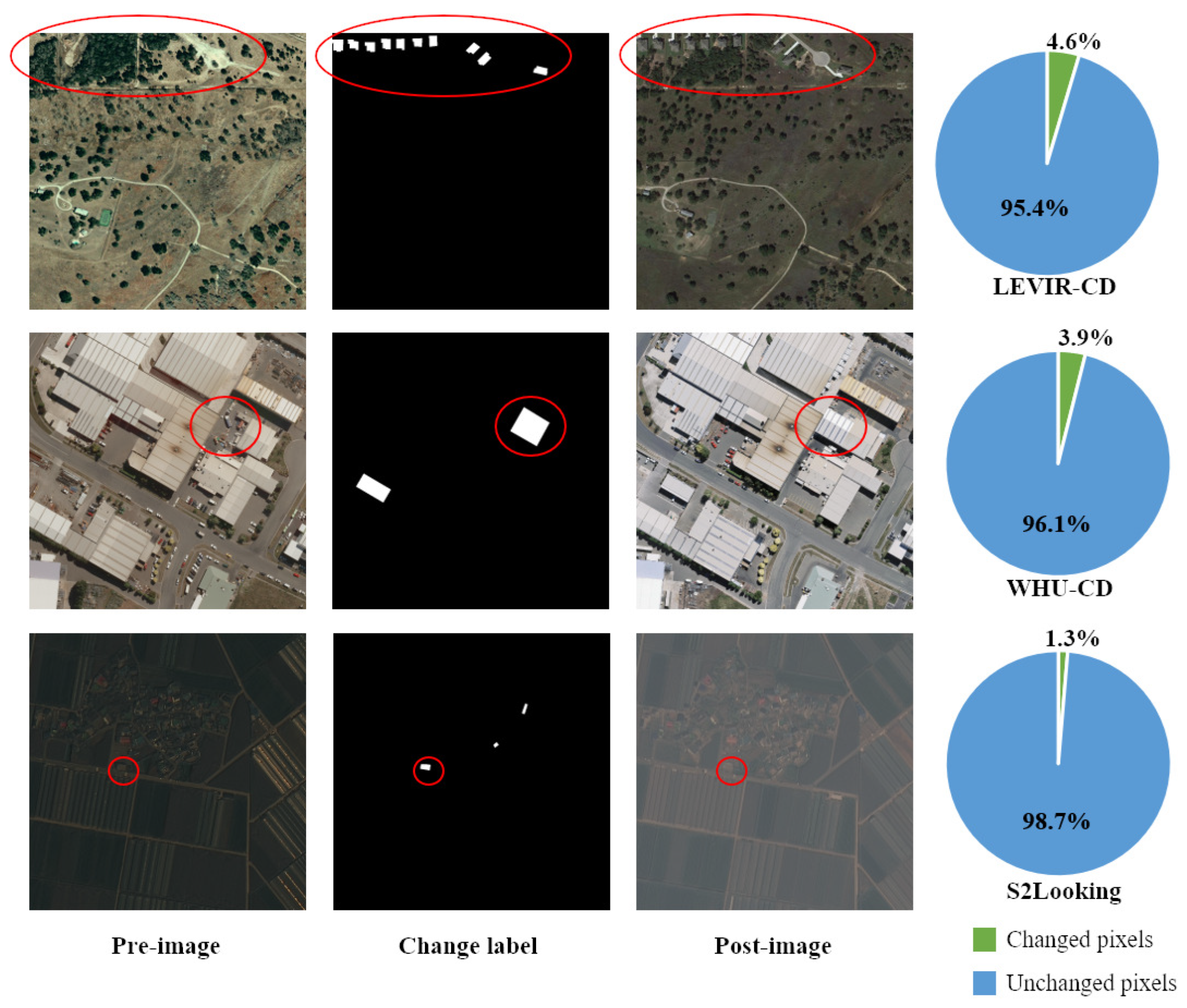
However, obtaining a large dataset of bitemporal remote sensing image pairs containing diverse building changes is challenging. Firstly, it is difficult to collect large-scale bitemporal image pairs due to the inconsistency between the occurrence of building changes and satellite observation periods. Furthermore, high-precision building change detection relies on labor-intensive and time-consuming pixel-level labeling with a limited amount of available data. Secondly, existing change detection datasets typically cover only a small area and limited historical observation time, which result in a lack of diversity in bitemporal image pairs. Thirdly, building changes typically occur at a low frequency. As demonstrated in Figure 1, compared to the unchanged regions, the changed regions generally comprise a significantly smaller number of pixels, resulting in a severe class imbalance between the changed and unchanged classes. Sliding-window-based detectors often encounter a substantial class imbalance between the background and target building changes. In some instances, the number of background windows can be up to 10 7 times higher than the number of target windows [14]. For LEVIR-CD [10], which is commonly used for building change detection, the building change samples are sparsely distributed. After the original images are cut into 256 × 256 patches, it contains 7120 bitemporal image pairs, but only 3167 of them contain change information, and the others are all unchanged images. Moreover, in the 3167 changed bitemporal image pairs, the proportion of changed pixels in the total image pixels is mostly less than 10 % . Such a class imbalance phenomenon will lead to the convergence process of the change detection model being biased toward unchanged samples, resulting in false alarms and missed detections, thereby degrading the performance of change detection.
The challenges of limited training sample pairs and class-imbalanced data are significant obstacles for building change detection models. Directly training a change detection model on such datasets may result in overfitting to specific types of changes and limit the model’s generalization capabilities. Furthermore, the class-imbalance issue renders accuracy an unreliable performance metric, as high training metrics for change detection models may not be applicable to images with different building appearances or image conditions in new geographical areas. One approach to address these issues is to develop a method for generating data that focuses on the fundamental problem: the dataset itself. This method posits that generating additional data may enable the extraction of more information from the original dataset and help mitigate overfitting. Expanding the training data and rebalancing the classes would provide a larger and more diverse set of examples for the model to learn from. This would aid the model in better comprehending the spectrum of potential inputs it may encounter during testing, ultimately resulting in enhanced performance when faced with novel, previously unseen data. In essence, by making the training set more comprehensive, we can reduce the gap between the training set and future testing sets, leading to the improved generalization performance of the model.
Typically, data generation methods can be categorized into two primary approaches: traditional transformation-based techniques [15,16,17] and GAN-based methods [18,19,20,21]. Traditional transformation-based methods include rotation, mirror image, horizontal flipping, random cropping, and the addition of noise to existing training samples [15,16]. This strategy is usually used to perform inpainting and copy and paste on a single temporal image to generate a new, changed temporal image, resulting in a pair of new bitemporal images [17]. Nonetheless, these approaches merely reorganize the original datasets without effectively enhancing their richness. Moreover, various GAN-based methods have been proposed to generate changed samples, such as buildings or cars, within the original image pairs. One approach is to use GAN-generated image patches, as seen in work by Kumdakci et al. [18]. Another method involves unsupervised CycleGAN for style transfer, as demonstrated by Jiang et al. [19]. To address the shortcomings of existing datasets, Rui et al. [20] developed mask-guided image generation models by employing GANs to create disaster remote sensing images featuring various disaster types and distinct building damages. Furthermore, Chen et al. [
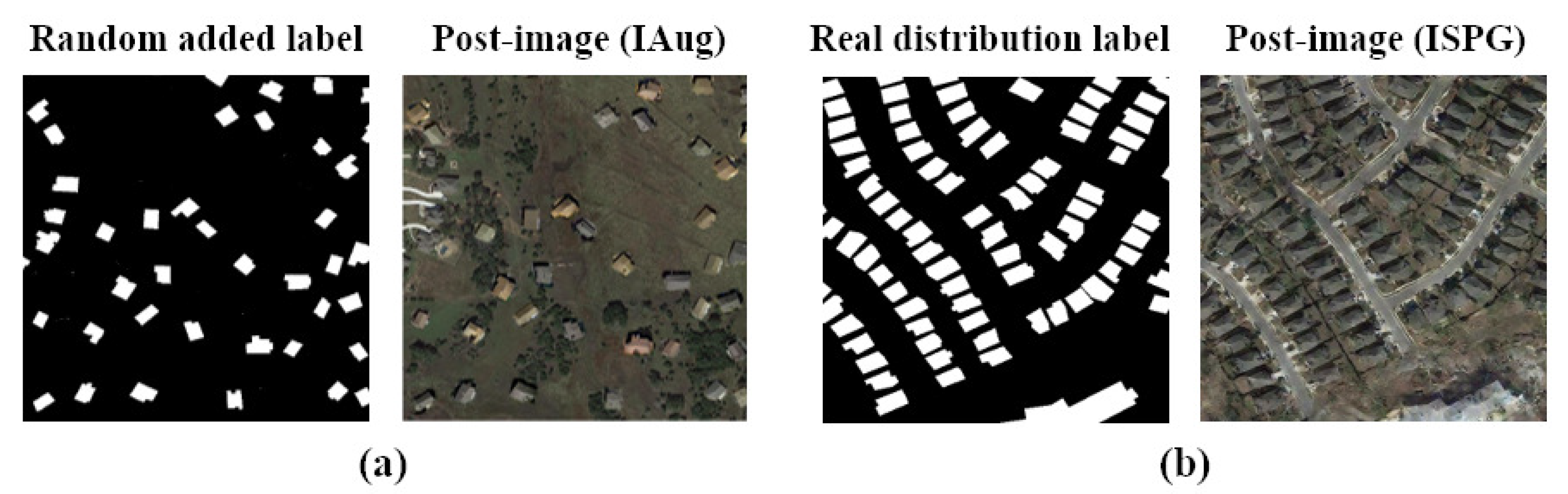
21] introduced an instance-level image generation model, termed instance-level change augmentation (IAug), capable of generating bitemporal images with numerous building changes. Although there are some methods for change detection data generation, these approaches have some limitations. Some involve several independent steps and require significant human intervention, making them less intelligent. Other methods rely solely on style transfer, and the generated sample pairs contain no new building instances, so they cannot address the issue of class imbalance mentioned before. Although some methods can generate entirely new building-instance-level changes, they may not produce building instances that look like real enough, or they may not reflect the actual distribution of buildings in the real world, which can be considered another type of unreality. Furthermore, most methods do not consider the importance of background pseudo-change generation for improving the data diversity.
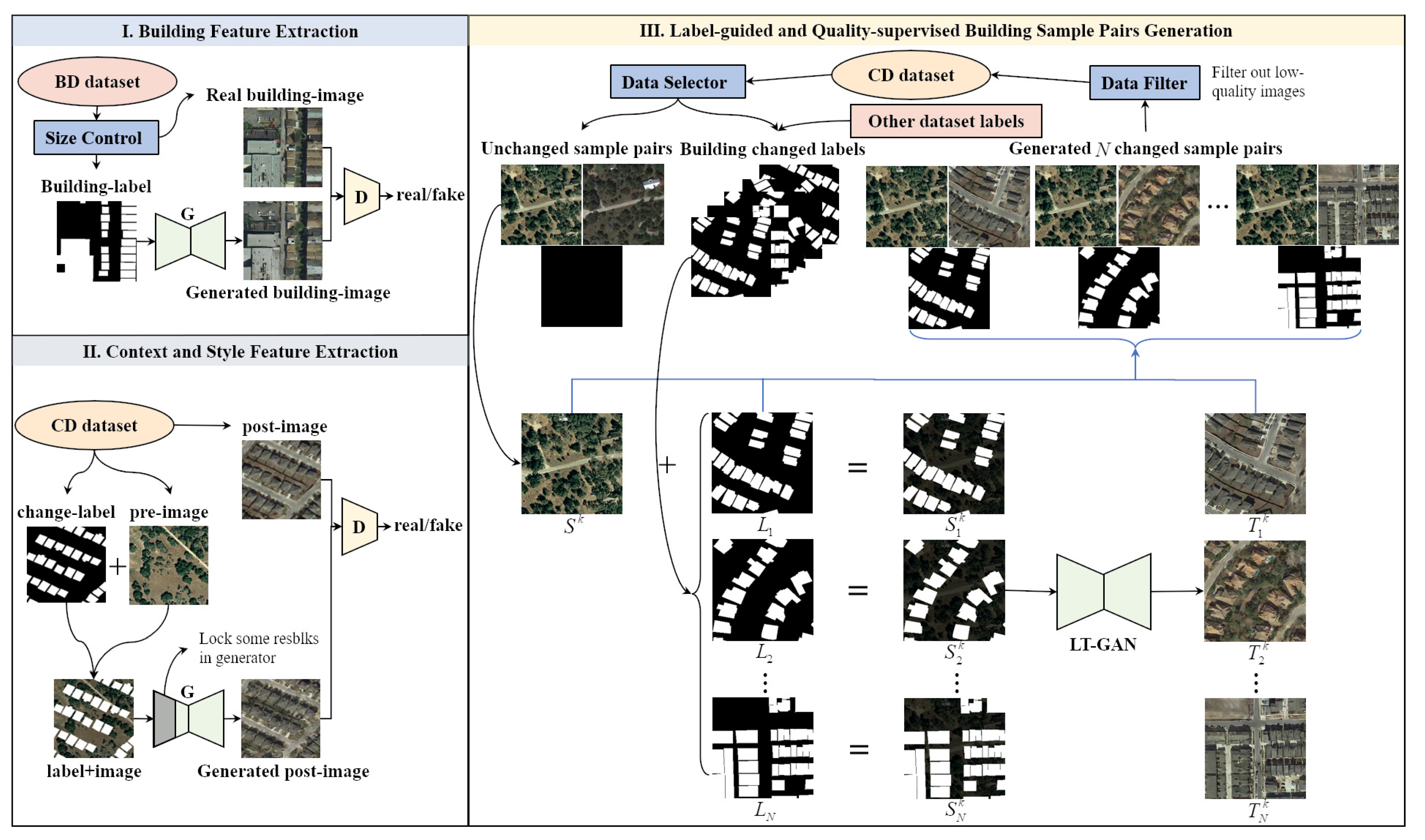
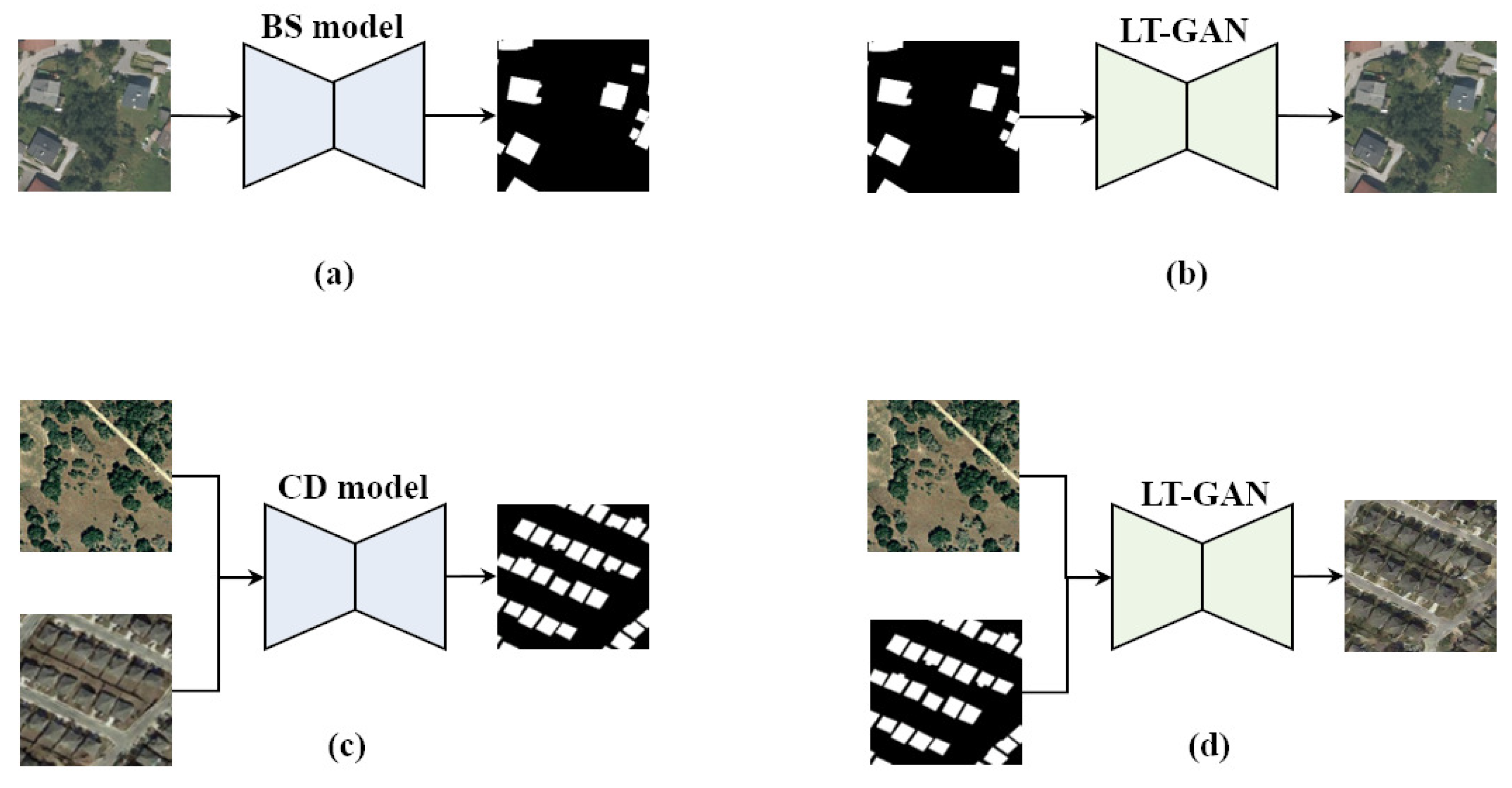
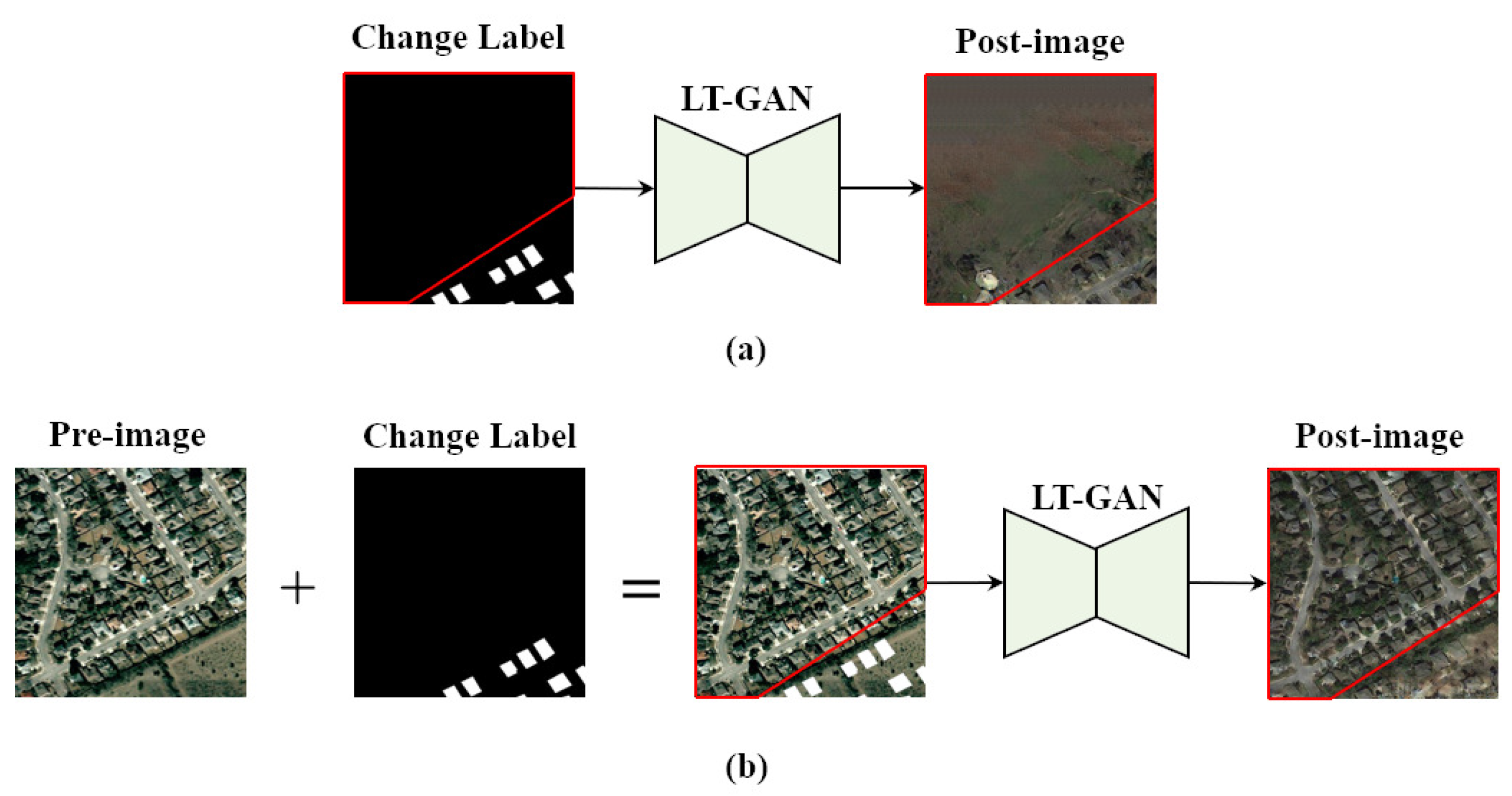
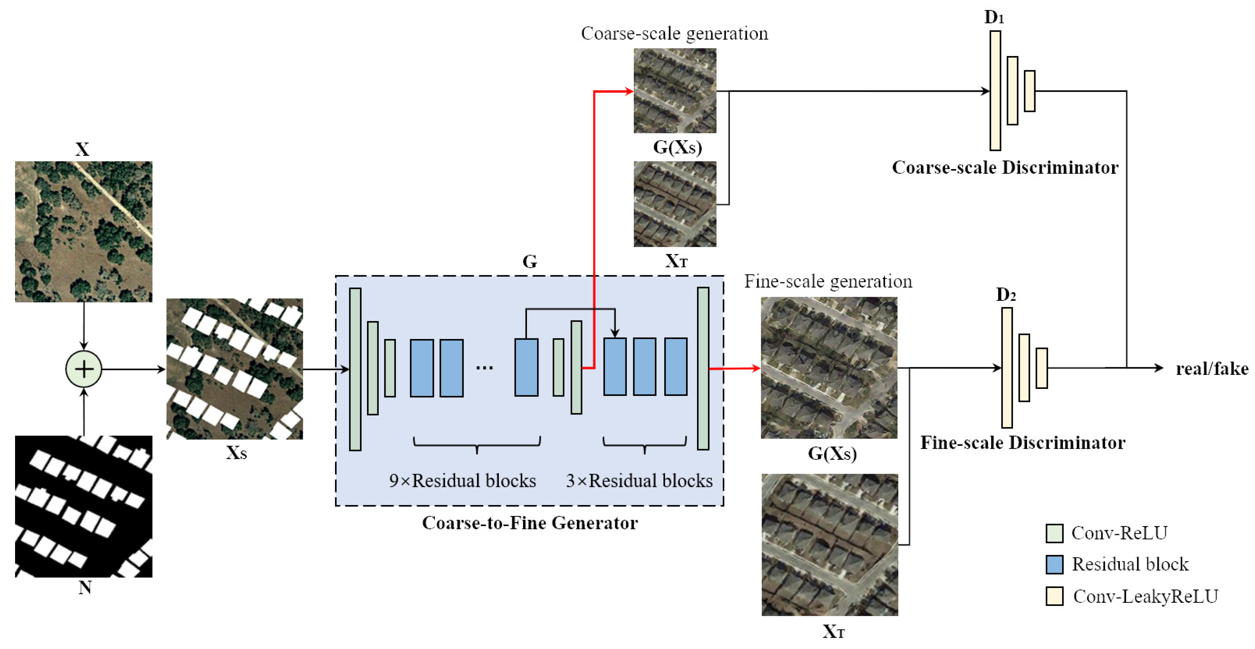
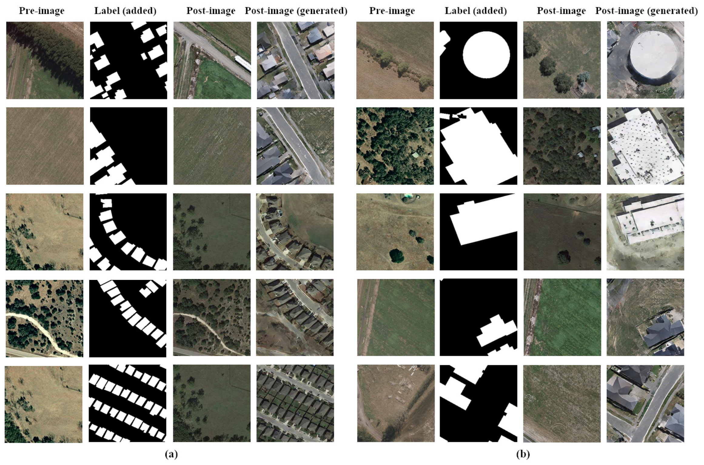
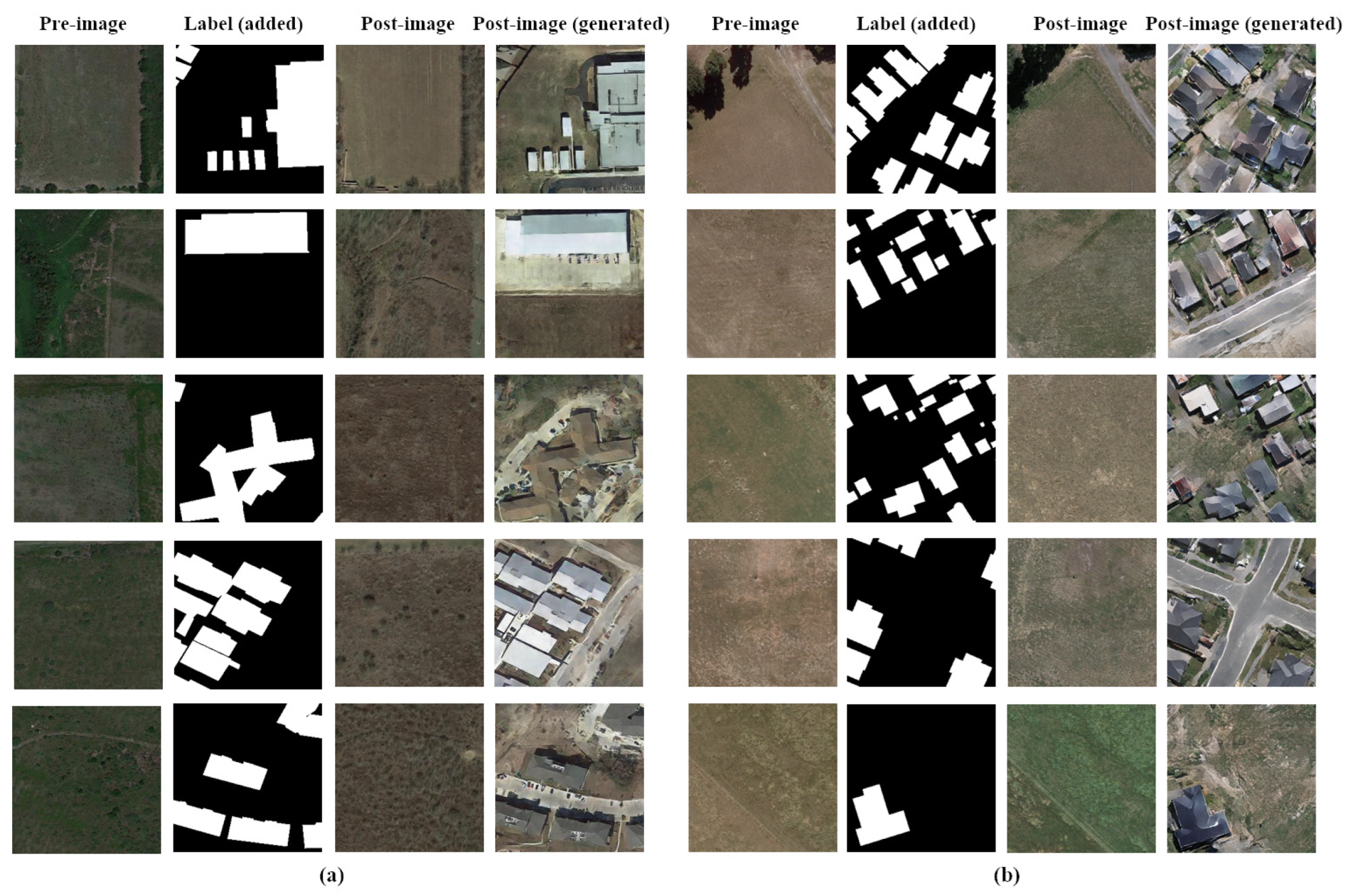
In this paper, we introduce a novel multi-temporal sample pair generation technique called Image-level Sample Pair Generation (ISPG) to enhance the building change detection performance. Our approach focuses on generating bitemporal sample pairs that include new types of building changes and pseudo-changes in the background. This addresses the challenges of limited data volume and severe class-imbalance issues. In order to simplify image generation and make it smarter, we did not design any color transfer or context-blending steps for properly pasting building instances into the original images but chose to design a Label Translation GAN (LT-GAN), which is a kind of Semantic Image Synthesis (SIS) technology, to realize the complete image-to-image translation between the building change labels and one of the bitemporal image pairs.
Since building change detection datasets suffer from limited data volume and class imbalance, these issues also affect the LT-GAN training process. Furthermore, LT-GAN is a data-hungry model that requires more paired data for training, making it unsuitable for direct training on change detection datasets. Fortunately, building segmentation datasets exhibit better class balance compared to building change detection datasets. This is because building changes necessitate time-period accumulation and are relatively low-probability events, whereas all existing buildings are labeled in building segmentation datasets. We can leverage this aspect to pretrain the encoder–decoder of LT-GAN and perform image-to-image translation with a greater number of building instances. With our sample pair generation strategy, LT-GAN extracts not only building detail features but also semantically related context features on other building segmentation datasets and then uses the change detection dataset to generate new sample pairs with abundant and diverse building changes with related pseudo-changes. To be specific, we use building change labels selected from the original dataset with any one of unchanged bitemporal sample pairs in the original dataset to generate other temporal images. On the other hand, LT-GAN can also generate semantically related instance-level pseudo-changes, such as roads and concrete floors, and style-level pseudo-changes, which help to improve the diversity of the generated data. Then, the generated images with more building changes form a series of class-balanced sample pairs. It is worth noting that different combinations of building change labels and unchanged sample pairs in the original dataset result in different new sample pairs with diverse and abundant building changes and pseudo-changes, so ISPG would greatly enrich the number and diversity of the original dataset and reduce the impact of the class-imbalance issue.
Compared with natural-scene images, remote sensing images are more complex, with various shapes and types of objects, different sizes, and various distributions. Therefore, building changes may appear at any scale and in any background. In order to generate various buildings and pseudo-changes and to ensure that the differently scaled objects generated have sufficient details to look realistic, LT-GAN adopts a coarse-to-fine generator with two discriminators at different supervision scales, which are the coarse scale and fine scale, to supervise remote sensing image generation. The coarse-scale discriminator with the largest receptive field would have better control over the global image generated, while the fine-scale discriminator with a smaller receptive field has better control over the image details. Different from the traditional GAN with one pair of a generator and discriminator, we use multi-scale adversarial loss (MAL) to train one generator with two discriminators at two scales of images. Conversely, to stabilize the adversarial generation training process for intricate and detailed building changes and pseudo-changes, we also employ feature matching loss (FML). This loss function helps suppress mode collapse during adversarial training and further enhances the quality of the generated sample pairs. Specifically, we extract feature representations from different layers for the two discriminators and calculate the loss function by comparing the feature differences between generated images and real images.
The primary contributions of this study can be summarized as follows:
(1)
We propose Image-level Sample Pair Generation (ISPG), which is applicable to building change detection datasets. To address the class-imbalance problem and expand the dataset, we leverage other labels with numerous building changes to introduce changes to the abundant unchanged sample pairs. Utilizing LT-GAN, we achieve image-to-image translation between labels and remote sensing images, thereby mitigating the impact of class imbalance.
(2)
We designed a GAN, namely, Label Translation GAN (LT-GAN), to efficiently synthesize new remote sensing images that contain changes involving numerous and diverse building changes and instance-level or style-level pseudo-changes in the background, which can improve the data diversity. Based on MAL and FML, it can generate complete and detailed remote sensing images end-to-end without manually editing or blending buildings into the background.
(3)
The method introduced in this paper offers a simple yet effective solution to the data scarcity problem in change detection. Our method and several existing CD methods were used for data augmentation on LEVIR-CD [10] and WHU-CD [22], obtaining better performance than the original dataset. Even the simplest change detection model with less raw data can achieve a performance better than or equal to state-of-the-art (SOTA) models. This plug-and-play solution has the potential to accelerate the development of the field of change detection by allowing researchers to work with smaller datasets and still achieve high accuracy.

2. Related Work

2.1. Change Detection

Change detection is a technique widely employed in various fields, including the monitoring of vegetation changes and urban expansion and the detection of illegal building construction. Traditional change detection methods, such as image differencing methods, often neglect the surrounding pixel information, resulting in high noise levels in the outcomes. In contrast, deep learning methods have emerged as powerful tools for feature representation in many applications, including object detection and semantic segmentation. As the volume of remote sensing data continues to grow, supervised learning methods are becoming increasingly popular in the field of change detection for remote sensing images. Two primary approaches exist for using deep learning in change detection. One approach is the post-classification method [23,24,25], in which a convolutional neural network (CNN) or fully convolutional network (FCN) is trained to classify each of the bitemporal images separately. The classification results are then compared to determine the change category. For example, Ji et al. [23] utilized an FCN to classify building pixels in each image and subsequently fed the binary building maps into a change detection network to generate a change map. The other approach involves training CNNs directly to produce a change map from the bitemporal images, eliminating the need for separate classification steps and potentially yielding more accurate results. Techniques such as the pixel-level approach [9,10,26,27] use FCNs to generate a high-resolution change map directly from the two input images, which is typically more efficient and reliable than the patch-level approach. From these recent works on deep-learning-based change detection, it can be concluded that advances have mainly focused on training with small labeled datasets, enhancing feature discrimination, and addressing class imbalance. Many works have aimed to improve feature discrimination by designing multilevel feature fusion structures [9,10,26,28,29], introducing self-attention mechanisms and attention modules, and incorporating GAN-based optimization objectives. To tackle the issue of small amounts of labeled data, transfer learning [30], active learning [31], and semi-supervised learning [32] have been adopted in recent work. The class imbalance in change detection is severe due to the intrinsically low frequency of changes in the real world. To address this problem, some researchers have focused on the model’s architecture itself, with weighted cross-entropy loss [33,34], weighted contrastive loss [10,27], and weighted dice loss [35]. In contrast to the techniques mentioned above, data augmentation approaches tackle overfitting from the root of the problem, the training dataset, which is discussed later.

2.2. Data Augmentation

Deep learning has achieved remarkable results in various computer vision tasks, such as image classification, object detection, and image segmentation. The success of these models can be attributed to the development of CNNs, advancements in deep network architectures, and access to large amounts of data. It is commonly believed that larger datasets lead to better deep learning models [12,36]. However, gathering massive datasets can be challenging, particularly for remote sensing images, and limited datasets can impede the generalization ability of deep learning models. Therefore, it is crucial to develop effective data augmentation techniques to address these challenges. Traditional data augmentation techniques typically involve applying geometric transformations or color space modifications to an existing dataset to generate additional samples. A new and exciting approach to data augmentation involves using generative modeling techniques to create artificial instances that closely resemble the original data. This method can help create a more comprehensive dataset, reduce the gap between training and validation data, and improve the performance on future testing sets. GANs, in particular, have been described as powerful tools for uncovering additional information from a given dataset [37].
Zhu et al. [38] expanded the original Facial Expression Recognition Database (FER2013 [39]) by applying CycleGAN. Due to the class imbalance in human emotions, the proportion of emotions such as anger and sadness is very low. It is important to use CycleGAN to generate expressions such as anger and sadness to expand the data and improve the classification model’s effectiveness. Frid-Adar et al. [40] tested the effectiveness of using DCGANs [41] to generate liver lesion medical images. Bowles et al. [37] used PCGAN to expand the brain region segmentation dataset and improved the accuracy of their DSC segmentation model by 1 to 5 percentage points under different conditions. Xuan et al. [42] developed a framework to generate data for change detection in water scenarios, improving the performance of supervised change detection models by using cycle consistency. DisasterGAN [20] employed GANs to synthesize disaster remote sensing images with multiple disaster types and different levels of building damage, addressing the class imbalance of existing datasets and the scarcity of training data. IAug [21] utilized generative adversarial training to produce bitemporal images containing changes in various buildings, enabling the detection of diverse changes. This article is inspired by the data augmentation work mentioned above and presents research on data augmentation in the field of building change detection. We propose the ISPG data generation method to enhance the metrics of building change detection models.

2.3. Generative Adversarial Networks

A Generative Adversarial Network (GAN) is a type of generative model that uses unsupervised learning to learn a probability density function from a training set and then generates new samples that are drawn from the same distribution [43]. GANs and their variants have demonstrated significant success in various computer vision tasks, such as image translation [44,45,46,47], facial attribute manipulation [48,49], scene generation [50], super-resolution [51,52], and semantic segmentation [53,54]. The original intention behind GANs was to develop deep learning from supervised to unsupervised, allowing computers to generate data that do not exist in the real world through imagination and creativity. GANs achieve this by pitting two neural networks against each other through a Min-Max game theory: the generator, which randomly samples from the latent space and generates fake samples through feature extraction and the corresponding encoder–decoder structure, and the discriminator, which is a binary classifier that distinguishes real from fake samples in the dataset [44].
Recently, GAN-based image-to-image translation tasks have attracted considerable attention from the research community [45,47]. Pix2pix [45] is a conditional adversarial network that provides a general-purpose solution to image-to-image translation by learning the mapping from inputs to outputs through paired images, enabling the same generic approach to be applied to problems that traditionally require different loss formulations. However, for some real-world tasks, paired training data may not be readily available or may not exist at all. To address this issue, CycleGAN [47] was proposed, which can perform style transfer between two different image domains, even if the images are unpaired. CycleGAN achieves cycle consistency by learning two mappings: G : X Y (from the source domain to the target domain) and the inverse mapping F : Y x (from the target domain to the source domain); cycle consistency loss ensures that F ( G ( X ) ) X .
Nevertheless, most of the results generated by CycleGAN are often limited to low resolution and are still far from realistic. Therefore, this paper proposes LT-GAN, which is designed to generate high-resolution remote sensing change detection image pairs with detailed information. LT-GAN improves upon existing GAN-based models by incorporating a Laplacian pyramid to capture more detailed information from the input images, resulting in more realistic and higher-quality output images.

2.4. Semantic Image Synthesis

Semantic Image Synthesis (SIS) is a challenging task with numerous practical applications in computer vision. Its goal is to produce photo-realistic images from given semantic maps, and it has become an important problem in various downstream tasks. Similar to how humans use past experiences as references to create new creations, the original idea behind generative adversarial network (GAN) design was to enable machines to have imagination and creativity. Early works on reference-based image synthesis, such as [55,56,57,58,59], studied this topic extensively. However, these methods relied on manual retrieval, stitching, and editing, which were sub-optimally optimized. To improve the quality of reference-based synthesized results, researchers began using deep neural networks such as SIMS [60]. SIMS takes the retrieved image as input, but it is limited in synthesizing complex real-world scenes. With the advancement of GANs, many methods based on GANs have been proposed to tackle SIS. The general framework for image-to-image translation proposed by pix2pix [45] enabled a wide range of applications, including SIS. However, the results were often limited to low-resolution images that were still far from being realistic. To overcome these limitations, pix2pixHD [61] improved the pix2pix framework by using a coarse-to-fine generator, a multi-scale discriminator architecture, and a robust adversarial learning objective function. With these enhancements, pix2pixHD can generate high-resolution photo-realistic images, even up to 2048 × 1024 , from semantic label maps. These developments inspired the creation of LT-GAN, which can generate detailed reference-based images for data generation.

3. Methods

In this section, we first address the necessity of generating image pairs containing numerous building-instance-level changes to tackle the class-imbalance problem in Section 3.1. Then, in Section 3.2, we provide an overview of ISPG, including the sample pair generation strategy and the generation model, LT-GAN. Section 3.3 offers a comprehensive introduction to the three steps involved in the sample pair generation strategy. Finally, Section 3.4 introduces the framework and objective function of LT-GAN, which is utilized in the strategy. Table 1 lists all the abbreviations of specific terms involved in the method. The code is available at https://github.com/MagicTerran0707/ISPG (accessed on 23 May 2023).

3.1. Motivation Clarity

Considering the real-world task of building change detection, one common challenge in this task is the class-imbalance distribution, where the number of unchanged instances significantly overwhelms that of change instances. This imbalance can pose a significant problem, particularly in training change detection models or data generation models, as it can lead to biased performance and reduced accuracy in detecting changes. So, building change detection datasets usually contain a large number of unchanged image pairs whose label maps are all zero, corresponding to the unchanged region in the original image. Therefore, it is necessary to generate building change image pairs containing a large number of instance-level building changes to compensate for the lack of change class samples in the dataset. Previous representative data generation methods such as copy and paste [62], generate and paste [21], style transfer [19], and cut and mix [17] cannot generate sufficiently realistic-looking RS sample pairs with plenty of building changes, and their problems can be summarized as follows:
  • Geographic location of building changes. It is worth noting that the geographical distribution of houses built by humans for production and living is not irregular. Most of them are built along roads, and the buildings are almost parallel to each other. Therefore, it is inadvisable and unrealistic to just randomly and evenly distribute generated buildings in the image. So, it is necessary to add building instances according to the distribution law of buildings in reality.
  • Diverse features of building changes. This question mainly aims to increase the diversity of building instances. This means generating as many new building types as possible, which should include, as much as possible, the validation set, test set, and any future building types that may appear in practical applications. In this manner, the change detection model’s performance can be enhanced, and the likelihood of overfitting can be mitigated to a certain degree.
  • Semantically related instance-level and style-level pseudo-changes in the background. It is essential to focus more on the generation of semantically related pseudo-changes in the background, an aspect that has often been overlooked in recent research. In our method, the pseudo-changes can be simply divided into instance-level and style-level. In normal circumstances, the surrounding context of new buildings built by humans cannot be completely unchanged. There are often roads and other related instance-level changes around several new buildings. This issue is also a situation that a building change detection model often faces in the training process, that is, to select interesting changed regions, which are building change instances, from numerous instance-level pseudo-changes, such as roads, trees, or lakes. In terms of style-level pseudo-changes in generated images, the post-image is also different from the pre-image, which is caused by the lighting, season, and other reasons. These style-level pseudo-changes represent a form of Strong Data Augmentation (SDA) for change detection models, aiding the model in differentiating between building-instance-level changes and building-style-level changes.

3.2. Overview

We propose a novel method called ISPG for generating building change detection sample pairs, including a sample pair generation strategy and Label Translation GAN. The sample pair generation strategy of ISPG, as shown in Figure 2, mainly consists of Building Feature Extraction (BFE), Context and Style Feature Extraction (CSFE) and Label-guided and Quality-supervised Building Sample Pair Generation.
  • Building Feature Extraction: LT-GAN is trained on a building segmentation dataset to extract more building features and semantically related context features. Due to the problem of class imbalance and insufficient data in the change detection dataset, which can also arise in the adversarial training of GANs, it is difficult for GANs to effectively generate building change areas. Instead of using masking or weighting strategies to guide the generation of these sparse change classes, as shown in the top left of Figure 2, we directly perform inverse training on a building segmentation dataset with more diverse building instances and balanced sample classes. Through labeled images, the high-generalization-ability generator can generate a sufficient number of diverse features of building changes.
  • Context and Style Feature Extraction: LT-GAN is fine-tuned on the building change detection dataset to extract background and style features. As there are still different style features between the building segmentation dataset and the change detection dataset, especially in the context of the buildings, merely using labels to generate images often results in generated context areas that lack realistic-looking objects or textures. Therefore, as shown in the bottom left of Figure 2, the change label and pre-image from each change image pair in the dataset are combined as the source domain image for training, and the target domain image is the post-image from the same image pair. This approach aims to train the generator to preserve the geospatial information in the unchanged context area and generate semantically related style-level and instance-level pseudo-changes in the context of the buildings.
  • Label-guided and Quality-supervised Building Sample Pair Generation: The positions of building instances generated need to comply with the distribution laws of the real world, and a reasonable building distribution can guide GANs to generate proper pseudo-change instances around buildings, such as roads, concrete floors, and grassland. Therefore, as shown in the third part of Figure 2, we use a data selector to split the changed sample pairs and unchanged sample pairs in the original building change detection dataset. In the bottom of this part, different combinations of pre-images, which are from unchanged sample pairs, and selected building change labels are used as inputs to the generator to perform the label-guided generation process, thereby constructing new pairs of change detection images. In the end, we further improve the quality of generated data by using a Data Filter based on IS and FID to filter out low-quality samples.
The three steps in the sample pair generation strategy rely on a common generative model, which is the Label Translation GAN (LT-GAN). We also provide a detailed introduction to LT-GAN in Section 3.4. In order to generate detailed and diverse building image sample pairs, LT-GAN consists of a coarse-to-fine generator with different residual blocks and two different scale discriminators to ensure the quality and detailed features of the generated images. Because of the effective sample pair generation strategy and the specialized generative model LT-GAN, ISPG can generate plenty of building change detection sample pairs end-to-end that contain diverse building changes with semantically related instances and style-level pseudo-changes surrounding the buildings.

3.3. Sample Pair Generation Strategy

3.3.1. Building Feature Extraction

For building change detection, the most important tasks are to extract effective building change information, decouple building change features and other pseudo-change features, and then generate corresponding building change labels. For the generation of building change image pairs, the most important tasks are similar, namely, to extract the geometric and style feature information of the building and then generate buildings with sufficient details and clear edges. In essence, the building change image pair generation method introduced in this paper is the inverse process of building change detection, as shown in Figure 3.
The inputs of the building change detection model are two remote sensing images of different time phases, and the output is a change label map, while LT-GAN generates the post-image, with the input being the combination of the pre-image and label. The common point for the two models is that both face the problem of an insufficient building change detection dataset and class imbalance, and compared with other deep learning models, the generation method based on GAN is even more data-hungry. If only the building change detection dataset is used to train LT-GAN, the issues that occur in the change detection model will also be reflected in the LT-GAN’s adversarial training. This can result in the generator being unable to adequately extract building features and generate images with sufficient detail and diverse building types. One approach to solving this problem is to use weight-mask-guided image adversarial training to increase the weight of the loss in the building change region in the image, which encourages the generator to focus more on the sparse building change samples in the dataset. However, our method directly addresses the problem itself, i.e., the class-imbalanced dataset. As depicted in Figure 2 (top left), we pretrained LT-GAN by utilizing another dataset similar to the building change detection dataset, specifically the building segmentation dataset. This dataset does not differentiate between changed and unchanged buildings, but rather labels all existing buildings within the image. This approach assists LT-GAN in extracting more detailed features of various building types and focusing on the distribution characteristics of multiple buildings as well as the semantically related context instances surrounding them. Additionally, the building segmentation label is similar to the binary label of the building change label, which is helpful for the subsequent conversion of LT-GAN between the two datasets. We also took into consideration the issue of varying the size of buildings between the two datasets due to differences in shooting platforms or satellite altitudes. Therefore, as shown in the top left of Figure 2, we use a size-control module to calculate the Average Pixel Area (APA) of the building labels between the two datasets. Based on this, we resized the building segmentation dataset accordingly by either reducing or enlarging the size of the data.

3.3.2. Context and Style Feature Extraction

After BFE, the generator also needs to be trained on the CD dataset to ensure that the context and style features of the generated image correspond to the change detection dataset. Since LT-GAN is based on SIS technology, it can translate the semantic label to the corresponding real-world image. On the other hand, the change detection label is also a kind of semantic label, so by inputting a building change label, the generator can produce the corresponding changed post-image to form a new image pair. However, there is still a big difference between the change label and the semantic label, which is that the change label has a large area of the unlabeled region because of the sparsity of the change class, which means that lots of pixels in the label are zero. If we only input this kind of label to generators directly, the geospatial information will be lost after passing through stacks of convolution, normalization, and nonlinear layers. This means that, in addition to the marked buildings generated in the post-image, other unchanged regions will lack any realistic-looking objects or textures, as shown in Figure 4, not to mention any instance-level pseudo-changes such as generated roads surrounding the buildings.
To address this issue, the change detection label cannot be used alone as an input image to generate complete building change detection sample pairs. In terms of the input–output relationship of the model, as shown in Figure 3, the inverse process of change detection originally requires a labeled image as input to generate two images from two different time phases. However, generating two images with rich details and additional building change instances is too complicated and unrealizable. Therefore, LT-GAN is trained to generate the post-image with the guidance of the labels, which can retain the style features of the dataset and unchanged buildings in the background, as shown in Figure 4. Specifically, as shown in the bottom left of Figure 2, we added a label to the pre-image of each remote sensing image pair in the change detection dataset to guide LT-GAN to generate corresponding building change instances at the corresponding label positions and produce instance-level and style-level pseudo-changes around the change instances. To retain the previously trained building features, we froze some residual blocks in the encoder to enhance the model’s learning of the style and background features in the change detection dataset and, at the same time, preserve the building feature layers previously trained on the building segmentation dataset.
This dataset transfer training makes LT-GAN learn to combine the joint information of the pre-image and label and generate the complete post-image. So, compared to previous methods of only generating buildings and directly pasting them in the post-image, we have more pseudo-changes around the change areas, such as new roads next to the new buildings, to make the generated post-images more realistic. This kind of post-image with instance-level pseudo-changes can be seen as a kind of SDA that assists the building change detection model in not recognizing the pseudo-change samples in the test set as building changes, further improving the accuracy of the CD model.

3.3.3. Label-Guided and Quality-Supervised Building Sample Pair Generation

In the previous two sections, we discussed how LT-GAN can be trained to generate a new remote sensing image of another time phase by inputting a label map and an arbitrary remote sensing image. This can be used to construct new building change detection image pairs to expand the dataset. However, random label maps pasted onto the image may not reflect the actual distribution of buildings in the real world. In reality, the distribution of buildings usually follows human construction habits, such as parallel edges between buildings, consistent building orientations, and consistent spacing between buildings. This distribution pattern of buildings also affects the distribution of semantically related instance-level pseudo-changes generated in the context of buildings. Therefore, generating building instances based on the actual distribution pattern is necessary to further enhance the realism and diversity of the generated sample pairs, as shown in Figure 5.
One approach is to train another GAN to learn the distribution pattern of buildings from the segmentation dataset and generate corresponding building label maps to guide LT-GAN to generate building change instances at the corresponding locations. Nonetheless, we propose a simpler and more effective approach by employing a data selector to segregate the changed and unchanged image pairs within the original dataset, as illustrated in the third part of Figure 2. Unchanged image pairs are the main source of class imbalance and require additional building change instances. Fortunately, the change image pairs contain label maps that follow the actual distribution pattern of buildings and can be used to guide the generation of building instances in the non-change image pairs. Furthermore, to improve the diversity of the generated building instance distribution, we also introduce other label maps from the segmentation dataset and appropriately scale the size of the added label maps to match the scale of the building change detection dataset. During the inference phase of LT-GAN in Figure 2, we only need to add these change label maps to any image of the unchanged image pairs to guide LT-GAN to generate building instances at the corresponding locations, as well as semantically related pseudo-changes around the building instances, and achieve the style transfer of the entire image. Taking LEVIR-CD as an example, 3167 building change labels and 3953 unchanged sample pairs are selected by the data selector from the original training set. The pre-image of unchanged sample pairs can be denoted as { S k , k = 1 , 2 , 3 , . . . , 3953 } , and we add random N label maps { L 1 , L 2 , . . . , L N } on S k . This process can be represented as ( S k , L i ) n o i s e S i k , as illustrated in Figure 2. Then, we input these N label-added pre-images { S i k , i = 1 , 2 , 3 , . . . , N } to LT-GAN to generate the post-images { T i k , i = 1 , 2 , 3 , . . . , N } , which correspond to the added labels { L i , i = 1 , 2 , 3 , . . . , N } . Finally, these N pairs of generated samples are adopted to expand the dataset. Note that different combinations of label maps can produce different change image pairs for each unchanged image pair, greatly enriching the types of building change sample pairs and improving the proportion of change class samples in the dataset. In order to further enhance the quality of the generated images, we employ a Data Filter, as depicted in the top right of Figure 2. This filter quantitatively evaluates the quality of generated images using IS and FID metrics, effectively filtering out image pairs with low generation quality and thereby further improving the image quality.

3.4. Label Translation GAN

In this section, we first provide an overview of the LT-GAN framework architecture, as illustrated in Figure 6. Following that, we delve into the details of LT-GAN’s objective function.
The framework architecture of LT-GAN consists of a generator G · and two discriminators D 1 and D 2 with different scales to discriminate the generated RS images, as shown in Figure 6. X denotes a pre-image from one unchanged image pair in the CD dataset. N denotes a corresponding building change label from the dataset, and X T denotes a corresponding temporal image from the same image pair. X S is formed by adding X and N. X S and X T denote the concept of the source domain image and target domain image in the image-to-image translation task. G ( X S ) refers to the generated post-images, which are discriminated with the real post-image X T by two discriminators at coarse and fine scales. The two groups of differently sized G ( X S ) and X T in Figure 6 represent images generated from a coarse-to-fine generator at different scales. The smaller images represent coarse-scale generation, while the larger images represent fine-scale generation, which contain more detailed texture features.
The generator’s network structure is based on Johnson et al.’s work [63], which has been proven to be an effective approach for style transfer. The generator G · is divided into coarse- and fine-scale generation stages, corresponding to two different numbers of residual block sets. In coarse-scale generation, there is a set of residual blocks and a corresponding convolutional front-end and transposed convolutional back-end. The input source domain image X S is composed of a building change label N and a certain temporal image X, passing through the three components and generating a target domain image at the coarse scale, including building instance generation guided by the building change label and corresponding pseudo-change generation. In fine-scale generation, the feature map of the convolutional front-end and the last feature map of the previous 9 residual blocks are element-wise summed and input into the three residual blocks of the fine stage. So, the coarse-to-fine generator further improves the combination of global and local image features and generates high-quality images.
In the two different generation stages of the generator, there are two discriminators D 1 and D 2 of different scales that discriminate between the generated image G ( X S ) and the real image X T at the corresponding scales to ensure that the features of the images at two scales sufficiently match the features of the real image. The coarse-scale discriminator has better control over the global image generated, while the fine-scale discriminator has better control over the image details. They receive the input of generated images at different layers of G · , which are marked with red lines in Figure 6. In the synthesizing phase, G ( X S ) composes new pairs of bitemporal images with different selected building change labels, which were mentioned before and are used to expand the building change detection dataset.
The objective function of LT-GAN includes three parts of the loss function, which are MAL, FML, and VGG perceptual loss, which have been commonly used before and are introduced below.
Multi-scale Adversarial Loss.
We employ an adversarial learning strategy to train the generator and discriminators simultaneously, making the generated post-images indistinguishable from the real ones. Our generator G · , as shown in Figure 6 and illustrated as a coarse-to-fine generator, aims to translate a mixed image of the pre-image and label into a realistic-looking corresponding post-image during training on the building change detection dataset. On the other hand, the discriminators D 1 and D 2 strive to differentiate the real post-images from the translated fake images. In contrast to unsupervised GANs, such as Cycle-GAN [47], which can be trained on unpaired datasets, our LT-GAN framework is a supervised GAN that requires a paired dataset for training. This means that training necessitates source domain images and target domain images with strictly corresponding semantic information. Fortunately, the building change detection dataset is intrinsically paired, where the pre-images’ semantic information is consistent with the post-images, allowing us to better train LT-GAN. In other words, the training set consists of building change sample pairs ( X S , X T ) , as depicted in Figure 6, with X S being the label-added pre-image. LT-GAN aims to model the conditional distribution of post-images given the input pre-images with change labels via the following minimax game:
min G max D L G A N ( G , D )
in which the objective function L G A N ( G , D ) is given by
L G A N ( G , D ) = E ( X S , X T ) [ log D ( X S , X T ) ] + E X S [ log ( 1 D ( X S , G ( X S ) ) ) ]
This basic objective function is used for image-to-image translation. To generate higher-resolution remote sensing images and enhance the quality of synthesized images, a discriminator with a larger receptive field is necessary. However, this would require deeper networks and larger convolutional kernels, potentially leading to overfitting or increasing the network capacity. Moreover, training such a GAN is challenging in reality, as it demands a larger memory footprint, which is already a scarce resource for remote sensing image generation. To address this issue, LT-GAN improves the discriminators’ objective function by incorporating multi-scale adversarial loss (MAL), which involves discriminating images at different scales. We denote the two different scales of discriminators as D 1 and D 2 , as shown in Figure 6. In practice, they downsample the real post-image X T and the synthesized post-image G ( X S ) to create a two-scale image pyramid. This means that the discriminators D 1 and D 2 are trained to discriminate real and synthesized post-images at two distinct scales, respectively. The coarse-scale discriminator D 1 possesses a larger receptive field, so it operates on images at the coarsest scale. This discriminator, which has a more global view of the image, guides the generator to create a post-image that is more globally consistent with the real post-image. Conversely, the fine-scale discriminator D 2 encourages the generator to produce finer texture features and detailed building instances in the generated post-image. With the improved discriminators mentioned, LT-GAN’s objective function can be considered multi-scale adversarial loss:
k = 1 2 L G A N ( G , D k )
Then, the adversarial training of LT-GAN becomes a multi-task adversarial training process of
min G max D 1 , D 2 k = 1 2 L G A N ( G , D k )
Feature Matching Loss.
In this section, we introduce feature matching loss based on the discriminators to enhance the GAN performance. This GAN discriminator feature matching loss is related to perceptual loss [64,65], which has proven beneficial for image super-resolution and style transfer tasks. In our context, this loss stabilizes the adversarial training process, which is more susceptible to mode collapse in general GAN training, especially during the multi-scale adversarial training process mentioned earlier. Additionally, it helps improve the quality of synthesized remote sensing images. Specifically, features are extracted from multiple layers of the two discriminators. Throughout the training process, LT-GAN learns to match these intermediate feature representations between the real and synthesized post-images. To present the objective function for this part more easily, the ith-layer feature extracted from the discriminator D k can be represented as D k i . Then, the overall feature matching loss L F M ( G , D k ) is given by
L F M ( G , D k ) = E ( X S , X T ) i = 1 T 1 N i [ | | D k i ( X S , X T ) D k i ( X S , G ( X S ) ) | | ]
where T is the total number of layers in the discriminators, and N i denotes the number of elements in each layer.
VGG Perceptual Loss.
We have also explored incorporating the VGG perceptual loss, which is commonly employed in other works. The objective function can be expressed as follows:
L V G G = λ i = 1 N 1 M i [ | | F i ( X T ) F i ( G ( X S ) ) | | ]
where λ = 10 , and F i · represents the ith layer with M i elements in the VGG network. This type of loss can also enhance the quality of the generated remote sensing images.
The full objective function of LT-GAN, which includes the multi-scale adversarial loss, feature matching loss, and VGG perceptual loss, is shown as below:
min G ( ( max D 1 , D 2 k = 1 2 L G A N ( G , D k ) ) + λ k = 1 2 L F M ( G , D k ) + L V G G )

4. Experiments and Results

In this section, we provide an overview of our experiments. Firstly, we introduce the datasets used in the experiments. Next, we describe the implementation details and evaluation metrics used to assess the performance of the change detection model. Secondly, we showcase the sample pairs generated in the building change detection dataset, which demonstrate the diverse building change instances and the instance-level and style-level pseudo-changes generated by ISPG. Thirdly, we present several quantitative experiments, the evaluation metrics of change detection models, and the visualization of the change detection results under different degrees of dataset expansion to validate the effectiveness of ISPG. Finally, we report an ablation study that we conducted to demonstrate the effectiveness of the proposed ISPG.

4.1. Datasets

Our research is based on LEVIR-CD [10] and WHU-CD [22], which are two open-source VHR building change detection datasets, and the Inria building dataset [66] and Aerial Imagery for Roof Segmentation (AIRS) [67], which are two open-source VHR building segmentation datasets.
  • LEVIR-CD [10]: LEVIR-CD is a collection of 637 pairs of large-scale bitemporal images, each with a resolution of 1024 × 1024 pixels and a spatial resolution of 0.5 m. The dataset is designed for building change detection tasks and contains over 31,000 building change samples. To accommodate GPU memory limitations, the dataset was split into three sets: training, validation, and testing. The default split is 445/64/128 for training/validation/testing. Additionally, to further reduce memory usage, the images were cropped into small patches with a size of 256×256 with no overlap. After cropping, the dataset consisted of 7120, 1024, and 2048 pairs of 256×256 patches for training, validation, and testing, respectively.
  • WHU-CD [22]: This dataset consists of one pair of large optical remote sensing (RS) images with a size of 32507 × 15354 and a spatial resolution of 0.075 m. Similar to LEVIR-CD [10], the large image was cropped into small patches with a size of 256 × 256 with no overlap, resulting in 7434 patch pairs. As the dataset did not come with a suggested split, we split it into 6034 / 700 / 700 patch pairs for training, validation, and testing, respectively.
  • Inria [66]: This dataset contains 4500 / 1500 / 2500 pairs of aerial RGB building-labeled images for training/validation/testing, each with a size of 512 × 512 and a spatial resolution of 0.3 m, which is similar to LEVIR-CD [10]. It has more than 210K building instances for training the model.
  • AIRS [67]: This dataset is an aerial image dataset that covers the area of Christchurch city in New Zealand at a resolution of 0.075 m, which is similar to WHU-CD [22]. It has 857 / 94 / 95 pairs of aerial RGB building-labeled images for training/validation/testing, each with a size of 10,000 × 10,000.

4.2. Experimental Implementation Details

LT-GAN was first trained on two public building semantic datasets to extract building instance features. On the other hand, because AIRS [67] is a low-altitude aerial RS image dataset, the sizes of the houses in the images are larger and do not match the sizes of the buildings in WHU-CD [22]. A size-control module was used, as shown in Figure 2, to scale them to match the building sizes in WHU-CD [22]. In the end, we collected 23,632/29,081 training images from Inria [66] and AIRS [67], respectively. Each sample, including a building segmentation label and a corresponding 256 × 256 RS image, was cropped from the provided image and label maps in the existing building datasets. We trained our building generators on these two training sets for 300 epochs, with the last 200 epochs for the linear decay of the learning rate. To match the resolution and building features between the building change detection datasets and the building segmentation datasets, the generator pretrained on Inria [66] was used for LEVIR-CD [10], and the other one that was pretrained on AIRS [67] was used for WHU-CD [22]. After the above phase, we needed to train our generator on the building change detection dataset, as shown in Figure 2. Taking LEVIR-CD [10] as an example, in the GAN training phase, 7120 pairs of bitemporal images in the training set were used to train the generator. The training epoch number was set to 200, with the last 100 epochs for the linear decay of the learning rate. In this phase of LT-GAN training, which is an image-to-image translation process, the source domain images were pre-images with the corresponding labels added, and the target domain images were the real corresponding post-images from LEVIR-CD [10].
LT-GAN, referring to the basic parameters of Pix2pixHD [61], was trained from scratch using the Adam solver with a learning rate of 0.0002 . The learning rate was kept constant for the first 100 epochs and then linearly decayed to zero over the remaining epochs. Weights were initialized using a Gaussian distribution with mean of 0 and a standard deviation of 0.02 . LSGANs [68] were used for stable training, which is a commonly used approach for training GANs. In all experiments, the weight λ was set to 10, and K-means clustering was performed with the value of K set to 10. All experiments were conducted on an NVIDIA TITAN RTX GPU with 24 GB of GPU memory.
In the building change detection experiments, the change detection models discussed in this paper were implemented using the PyTorch Deep Learning framework and trained on a single NVIDIA TITAN RTX GPU. During the training phase, the CD models received images with a size of 256 × 256 pixels as inputs, and Stochastic Gradient Descent (SGD) with momentum was employed for training.

4.3. Evaluation Metrics

To quantitatively evaluate the proposed approach, we first used the F 1 score ( F 1 ), which is a commonly used evaluation metric for measuring the performance of change detection models. In our experiments, F 1 was calculated from the precision and recall of the test set. It can be represented as:
F 1 = 2 r e c a l l 1 + p r e c i s i o n 1
On the other hand, we also used Intersection over Union ( I O U ), which is a common evaluation metric used to measure the accuracy of change detection and segmentation. A higher I O U value indicates a better overlap between the predicted and ground-truth change regions and thus a more accurate prediction. I O U can be represented as:
I O U = 1 r e c a l l 1 + p r e c i s i o n 1 1
Let T P denote the number of true positives, F P represent the number of false positives, and F N indicate the number of false negatives. The definitions of precision and recall in the formula are given as follows:
p r e c i s i o n = T P T P + F P
r e c a l l = T P T P + F N

4.4. Sample Pair Generation Results

In order to verify the effectiveness of ISPG, we visualized the generated results. As shown in Figure 7 and Figure 8, each group consists of four columns of images, which are, respectively, the pre-image, added label, post-image, and generated post-image. In Figure 7a, the generated images contain building change instances that follow the human construction distribution, and there are corresponding instance-level pseudo-changes around the buildings, such as roads and concrete floors, which make the generated change detection images more realistic and diverse. It is worth noting that the context pseudo-changes are logically semantically related to the generated buildings because the building position distribution is realistic. In the fourth row, the pre-image has a dirt road, while the generated post-image still contains some trace of this road. This proves the effectiveness of using the change label and one temporal image as a combined input to LT-GAN. In Figure 7b, we show various types of generated buildings, including different shapes, such as the circle shown in the first row and the large polygon in the second row, and a few generated building instances. As can be seen, even the larger buildings shown in the second and third rows still contain some detailed texture, rather than simply being a big block. The different shadow shapes caused by the different shapes of the buildings also match well. These all help to further increase the diversity of the change detection images, making data augmentation for change detection more effective.
In Figure 8a, we show several special buildings generated in LEVIR-CD [10], including factory buildings and irregular building shapes, such as the snake-like shape shown in the third row. In Figure 8b, we generated buildings with differently colored roofs in WHU-CD [22]. In the first three rows, their added labels are from other datasets, resulting in very small buildings generated in the post-image. Moreover, in both (a) and (b), the generated post-images maintain consistent global style-level pseudo-changes with the post-image in the original dataset. For example, (a) maintains a corresponding desert style, and (b) maintains a grassland style.

4.5. Improvement of Change Detection Model

To evaluate the efficacy of the proposed data generation method, ISPG, and to compare the performance of various CD models under different data conditions, we established several data regimes: 5 % , 20 % , and 100 % . These percentages signify the proportion of training data employed in each data condition, simulating scenarios with very scarce, relatively scarce, and sufficient datasets, respectively. We used ISPG to perform data generation for different CD network structures to test the generality of our data generation method. On the other hand, we also checked the performance of our sample pair generation method by comparing it with some SOTA CD models. The dataset used in this experiment was LEVIR-CD [10], which was expanded by ISPG, in which the hyperparameter N = 5 . We also compared IAug’s [21] improvement to their CDNet [21].
  • FC-EF [8]: This is an image-level fusion method. The bitemporal images are concatenated and input into the FCN.
  • FC-Siam-Conc [8]: This feature-level fusion method employs Siamese encoders, and the fusion of features from the two branches occurs through concatenation.
  • FC-Siam-Diff [8]: This feature-level fusion method also utilizes Siamese encoders, but the fusion of features from the two branches is based on differences.
  • STANet [10]: This metric-based Siamese FCN method incorporates a spatial–temporal attention mechanism to extract highly discriminative features from the input data.
  • SNUNet [11]: This method adopts a densely connected Siamese network to alleviate the loss of localization information and employs the Ensemble Channel Attention Module (ECAM) for deep supervision.
  • CDNet+IAug [21]: This instance-level change augmentation method utilizes a simple yet effective CD model, namely, the CD network (CDNet).
Table 2 and Table 3 show the performance improvement of several typical change detection methods using only original data and data generated by ISPG. We present the improvements in four performance metrics: recall, precision, IOU, and F1, with the highest numbers in black. The first three change detection models, FC-EF [8], FC-Siam-Conc [8], and FC-Siam-Diff [8], are relatively simple and plain change detection frameworks. Furthermore, we also used the simplest resnet18 as the encoder, which results in poor performance with the original datasets. However, after sample pair generation by ISPG in which the hyperparameter N = 5 , even these simple change detection models show good performance, approaching the SOTA level with both LEVIR-CD [10] or WHU-CD [22]. The latter two change detection models, STANet [10] and SNUNet [11], are SOTA-level change detection networks. They can achieve good performance metrics without data augmentation, thanks to their carefully designed model architecture and attention mechanisms. It can be seen that even SOTA change detection methods achieve better performance with ISPG data augmentation, demonstrating the effectiveness and versatility of ISPG as a change detection data generation method. Additionally, we simulated the performance improvement under different data scarcity conditions by using three proportions of raw data, 5%, 20%, and 100%. It can be seen that ISPG can play a greater role in enhancing the performance of CD models when the data are more scarce, particularly at 5% and 20%. Finally, we also list CDNet [21] with the IAug developed by the same authors [21] to add extra data. In Table 3, when using 20% of the original data from LEVIR-CD [10], the first three simple change detection networks we used have poorer performance compared to CDNet [21]. However, after applying our ISPG data augmentation, the performance of these three inferior networks improved to a level comparable to CDNet [21] using IAug [21] for data augmentation, demonstrating the effectiveness of our method. Furthermore, when using 100% of the data, we were able to improve the performance of FC-Siam-Conc [8] to a level exceeding that of CDNet+IAug [21], despite the fact that FC-Siam-Conc’s [8] performance using the original data is lower than CDNet’s [21]. Table 4 lists the number of model parameters (Params.), floating-point operations per second (FLOPs), and the GPU inference time of the compared change detection models. The input to the model has a size of 256 × 256 × 3 . The reported time is the average of the inference time of the model for 100 random inputs. The results show that ISPG can effectively improve the performance of lightweight change detection models. Although they consume less computational resources, they can achieve a performance comparable to more complex change detection models through dataset expansion.
Figure 9, Figure 10, Figure 11 and Figure 12 show the visualized change detection performance improvement of FC-EF [8], FC-Siam-Conc [8], FC-Siam-Diff [8], STANet [10], and SNUNet [11] using 20% of LEVIR-CD [10] and WHU-CD [22] and the ISPG data generation method with the hyperparameter N = 5 . In Figure 9 and Figure 11, the results were obtained by directly training on the original LEVIR-CD [10] and WHU-CD [22], respectively, while Figure 10 and Figure 12 show the results obtained after training with ISPG data augmentation. It can be seen that, in the case of scarce data, three simple change detection models can hardly provide correct change detection results, while STANet [10] and SNUNet [11], due to their complex structural designs, can adapt to such small datasets but still have some issues with detection accuracy.
In particular, on LEVIR-CD [10], as shown in Figure 9, all models exhibited varying degrees of missed detections of changed buildings. The three simple change detection networks demonstrate high rates of missed detections of changed building samples due to the scarcity of the training data and class imbalance. On WHU-CD [22], as shown in Figure 11, the three simple change detection networks continued to exhibit high rates of missed detections of changed samples. However, STANet [10] and SNUNet [11] showed higher rates of false positives and had difficulty accurately delineating the edges of changed buildings. Furthermore, in the fourth row, STANet [10] shows completely missed detections of building changes with larger sizes.
After using ISPG data augmentation, all models showed improved performance, as shown in Figure 10 and Figure 12, with the three underperforming simple change detection models benefiting the most. These models went from almost unable to detect any building change areas to being able to detect almost every building change area, with visual performance approaching that of the SOTA network STANet [10]. The visual performance improvement on LEVIR-CD [10] and WHU-CD [22] can be seen in Figure 10 and Figure 12, respectively. WHU-CD [22] has more complex building changes, so the three simple change detection networks in Figure 11 could hardly detect any complete building change areas, while the simple change detection networks trained with ISPG could detect almost every building change area, as shown in Figure 12. This comparison illustrates the effectiveness of ISPG for improving the performance of basic change detection models.
On the other hand, the two SOTA-level change detection networks, STANet [10] and SNUNet [11], also show some visual performance improvement. On LEVIR-CD [10], in Figure 9, although the SOTA models could detect every building change area, some areas had some defects and missed detections, while the models trained with ISPG data augmentation detected more complete building change areas, as shown in Figure 10, with better edge detail processing. On WHU-CD [10] in Figure 11, both SOTA change detection models have serious false detection areas, while the models after ISPG data augmentation in Figure 12 have significantly fewer false detections and produce more precise change area edges, illustrating the effectiveness of using ISPG data augmentation for improving SOTA change detection models.

4.6. Ablation Study

Finally, we illustrate the effectiveness of the sample pair generation strategy of ISPG, as shown in Table 5. The extra data we added to the original training set are similar (about 4000 pairs of generated bitemporal images). The original training set used for all experiments in Table 5 is 20% of LEVIR-CD [10] (1424 pairs of images). The change detection model used is FC-Siam-Conc [8], and the hyperparameter N = 5 is used for the ISPG data generation strategy.
The first two rows in Table 5 are the comparison experiments. The first row shows the FC-Siam-Conc [8] model trained on the original 1424 pairs of change detection images without any data augmentation. The second row shows the change detection model trained after adding four times the original sample pairs as generated sample pairs. The high amount of redundant data led to overfitting, resulting in high precision but extremely low IOU and F1 score. The third row shows the change detection model trained using IAug [21], in which buildings are pasted at corresponding positions in the images. It is worth noting that for all experiments after this row, the selected labels added to the pre-image or the labels used to paste buildings are the same ones. This can ensure the fairness of the comparison experiments and prevent differences caused by different selected labels.
The following three groups of experiments are ablation experiments that verify the effectiveness of steps in the ISPG data generation strategy. The ISPG sample pair generation strategy includes three parts. The first two steps are the training processes of LT-GAN. The first step, BFE, aims to increase the variety of buildings generated by LT-GAN and address the problems of data scarcity and class imbalance in change detection datasets to improve LT-GAN’s generalization ability and generate higher-quality remote sensing images. Using only BFE improves the metrics compared to pasting buildings. The second step, CSFE, aims to synthesize another temporal RS image by combining the information of the label and the RS image, enabling LT-GAN to better adapt to the change detection dataset for data generation. Using only CSFE resulted in slightly higher metrics than using only BFE, indicating that there are style feature gaps between different building datasets, and using a generator trained on another dataset without considering this could lead to a performance drop on a building change detection dataset. The last row shows the ISPG data generation method using both BFE and CSFE. It achieved a significant improvement in IOU and F1 scores compared to the previous data generation methods, demonstrating the effectiveness of the ISPG image pair generation strategy.

5. Discussion

Based on LEVIR-CD [10] and WHU-CD [22], we constructed several synthesized training sets with varying imbalance ratios by using different hyperparameters N in ISPG. We define the imbalance ratio as the proportion of the number of pixels belonging to the unchanged class to the number of pixels in the changed class. The imbalance ratios of the original training sets and the corresponding synthesized training sets in LEVIR-CD [10] and WHU-CD [22] are listed in Table 6.
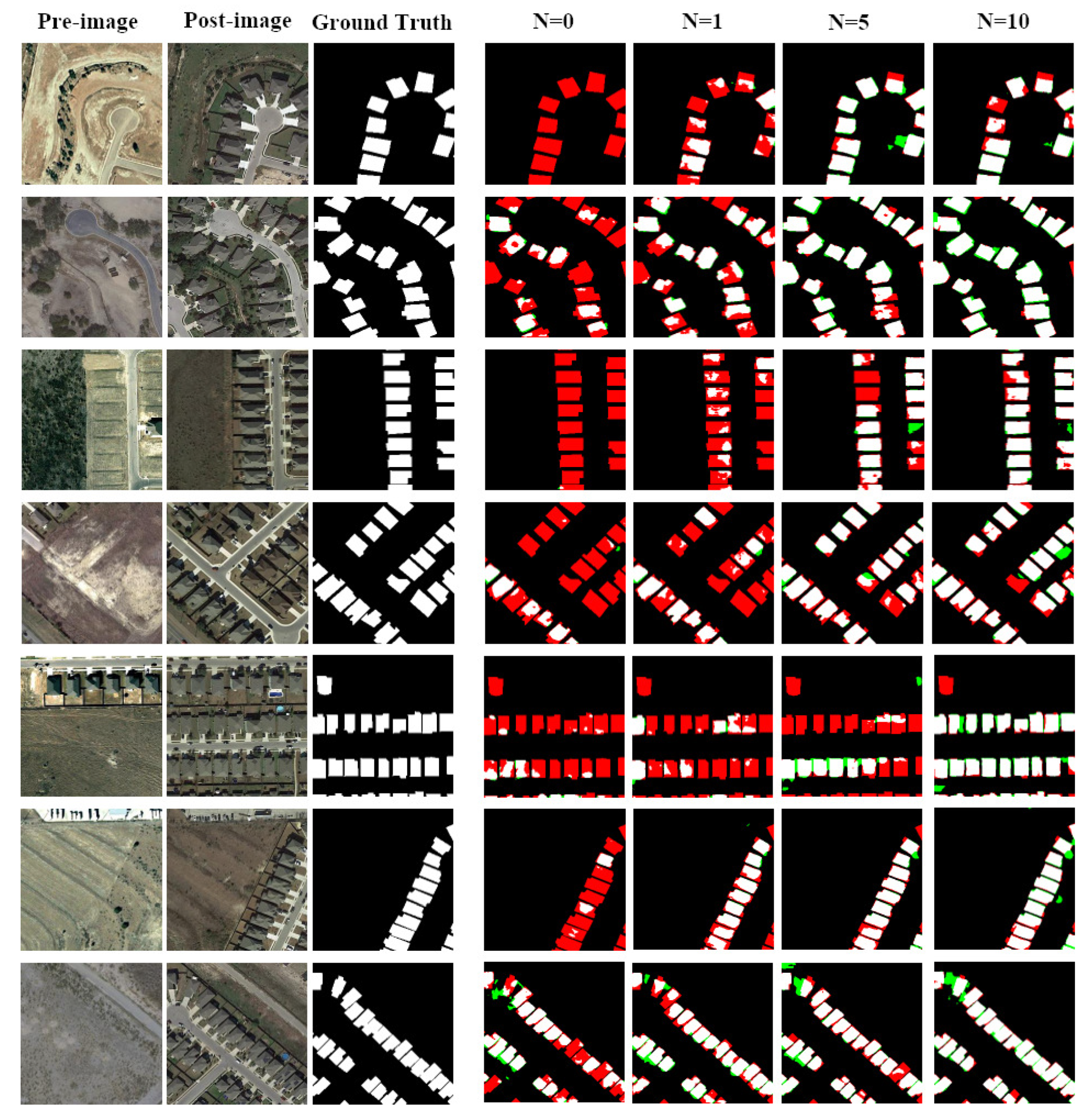
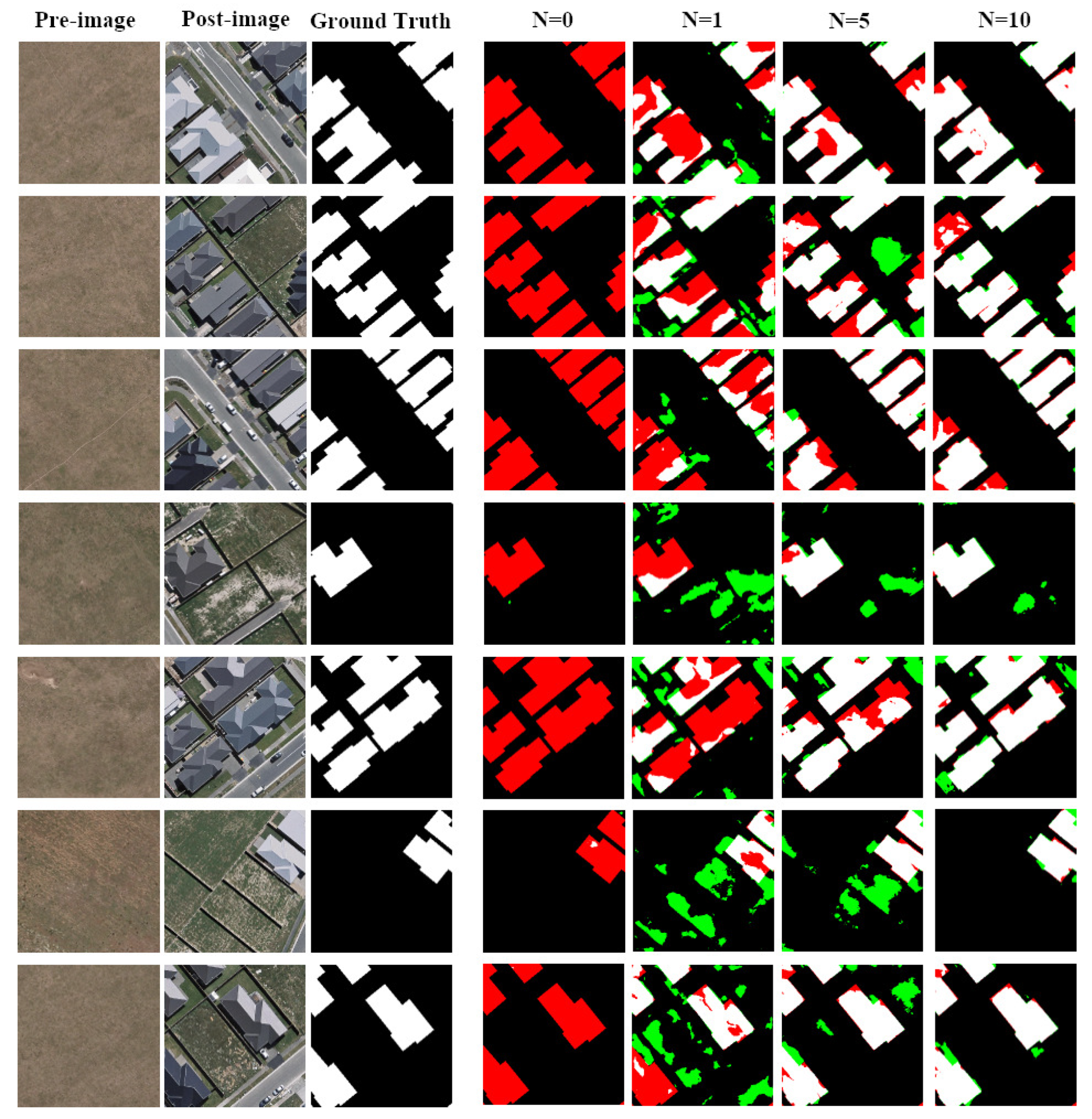
The quantitative results of different hyperparameters N in LEVIR-CD [10] are listed in Table 7, and those in WHU-CD [22] are listed in Table 8. The change detection model used is FC-Siam-Conc [
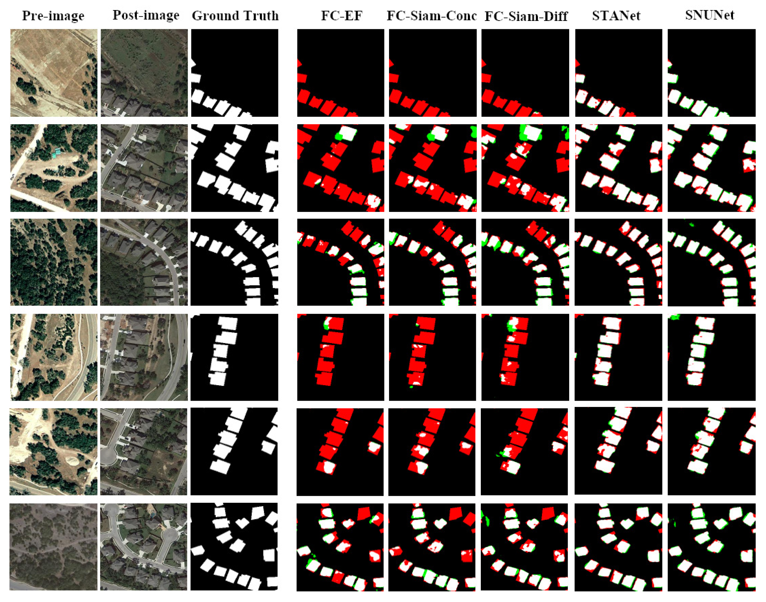
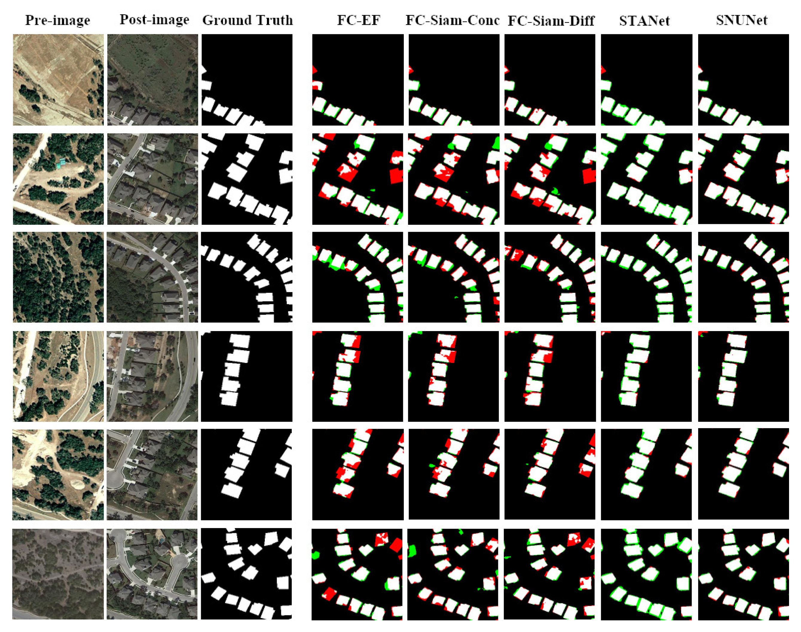
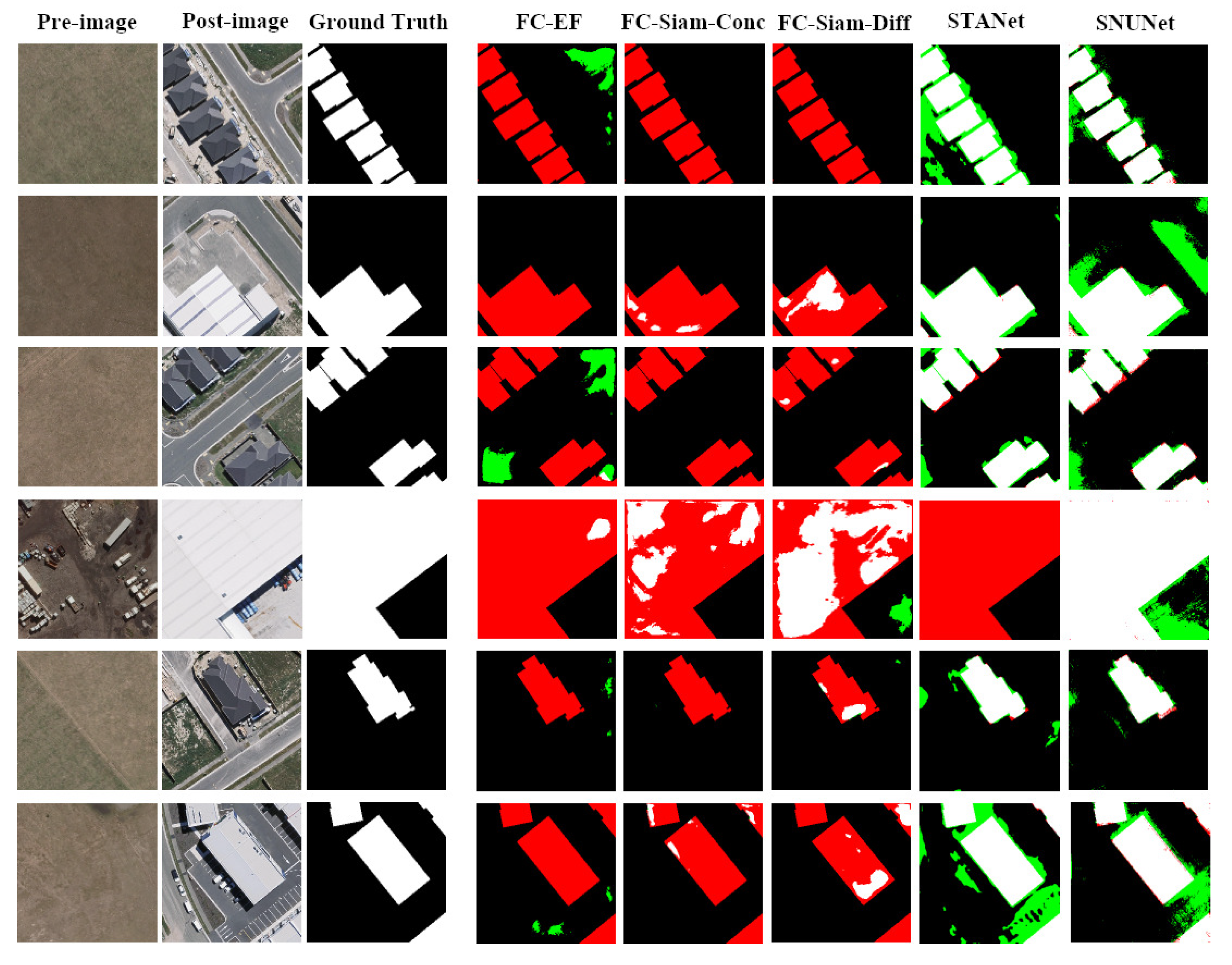
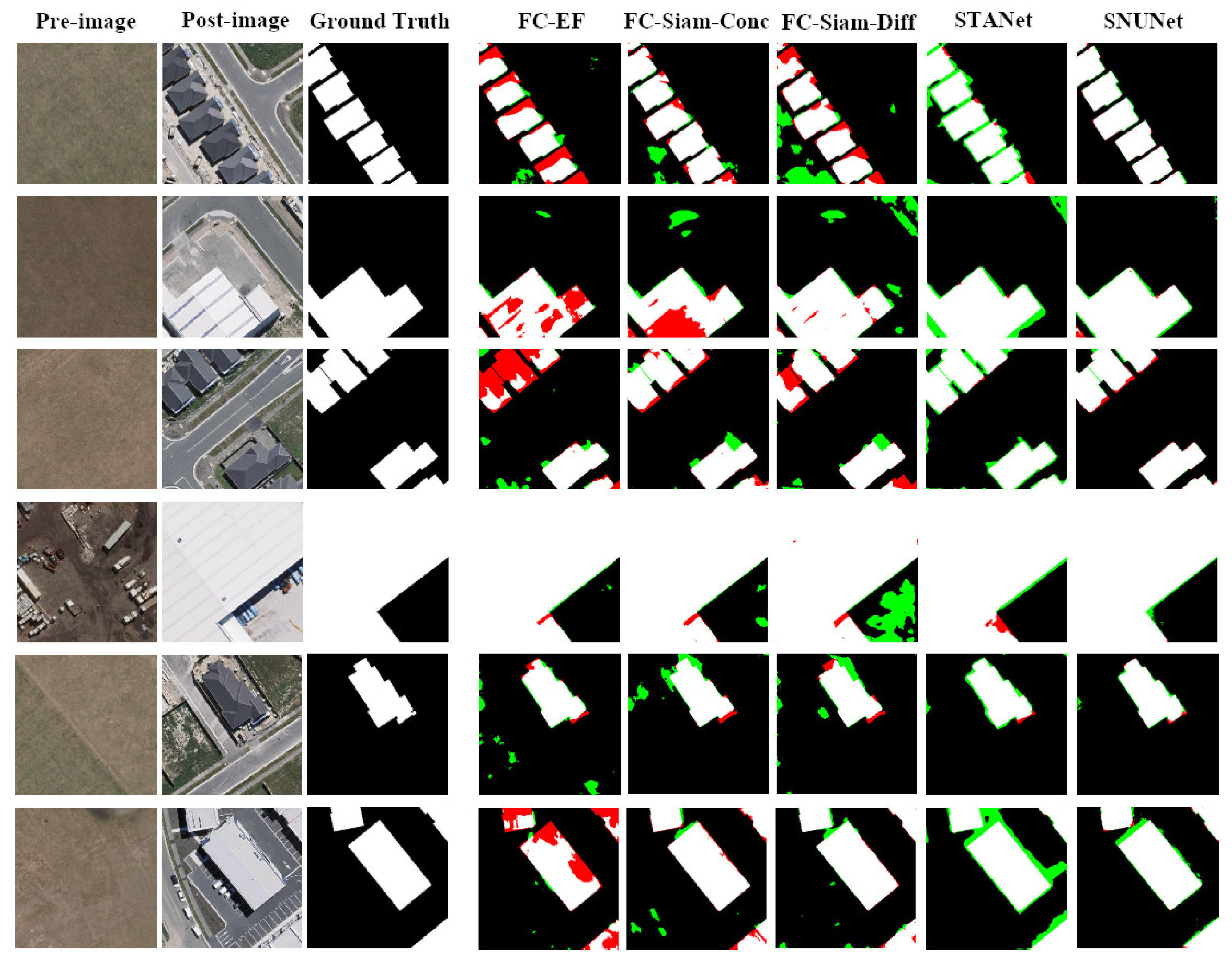
8]. Visual comparisons of LEVIR-CD’s [10] and WHU-CD’s [22] change detection results after using different hyperparameters N of ISPG are shown in Figure 13 and Figure 14, respectively.
From Table 7 and Table 8, it can be seen that by increasing the value of the hyperparameter N in the ISPG method, the imbalance ratio of the training set gradually decreases and the performance of the change detection model improves as the amount of data used varies (5%, 20%, and 100%) in different datasets (LEVIR-CD [10] and WHU-CD [22]). This indicates that ISPG can effectively reduce class imbalance in the dataset and that class imbalance in the dataset greatly affects the performance of the change detection model. When using 5% and 20% of the data, there are fewer imbalanced sample pairs in the dataset, so using ISPG with N = 5 or N = 10 leads to similar performance improvements. However, when using 100% of the data, there is a severe class-imbalance issue, so using ISPG with N = 10 results in a more significant performance improvement compared to using N = 5 . This further demonstrates the effectiveness of ISPG in addressing the problem of imbalanced building change detection datasets.
It should also be noted that when the dataset is very limited, such as when only 5% of the original data are used, the performance of ISPG with the hyperparameter N = 10 is lower than that with N = 5 or N = 1 . This may be due to the limited building change labels used in ISPG, resulting in too many identical distributions of buildings being generated. To further improve the diversity of data augmentation using ISPG in extremely limited datasets, it is suggested to consider introducing change labels from other datasets to generate different distributions of building instances.
Conversely, when the dataset is more sufficient, such as when 100% of the original data are used, the hyperparameter N in ISPG can be increased to fully unleash its data augmentation performance. At this time, the different ways of combining change labels and unchanged image pairs in the third step of ISPG will increase exponentially, and more effective generated image pairs can be obtained to improve the model performance.

6. Conclusions

In this paper, we propose a novel approach, Image-level Sample Pair Generation (ISPG), to tackle the data scarcity and class-imbalance issue in building change detection datasets. The proposed method generates valid multi-temporal sample pairs using a Label Translation GAN (LT-GAN) that generates complete remote sensing images with diverse building changes and background pseudo-changes. To improve the quality of generated image pairs, we designed multi-scale adversarial loss (MAL) and feature matching loss (FML) to supervise the surrounding context of the buildings. We also considered that the distribution of building changes generated should be consistent with building distributions in reality. To evaluate the proposed approach, several experiments were carried out on two building change detection datasets, LEVIR-CD [10] and WHU-CD [22], and state-of-the-art performance was achieved, even when using plain models and limited data for change detection. The experiments also illustrate that ISPG is a plug-and-play solution that can be used to enhance the performance of any change detection model. In conclusion, our proposed approach, ISPG, can overcome the limitation of small amounts of change information and the class-imbalance issue in existing building change detection datasets by generating more valid multi-temporal sample pairs. The generated sample pairs can improve the performance of building change detection models, which is crucial for identifying changes in the Earth’s surface for various applications. Current change detection data generation methods often involve generating instance-level image patches and then pasting and fusing them into the original images, without considering the generation of semantically related pseudo-changes. Semantic Image Synthesis (SIS) can achieve image translation from semantic segmentation maps to real-world remote sensing images. Therefore, we can edit the positions and shapes of different types of ground object targets in the segmentation labels to generate entirely new remote sensing images. In recent years, the diffusion model has shown better generative performance compared to GANs. We plan to further explore new methods and models in the remote sensing image generation field based on these two points in the future.

Author Contributions

Conceptualization, Y.L. and H.C.; data curation, Y.L., S.D. and Y.Z.; software and validation, Y.L.; formal analysis, Y.L. and H.C.; writing—original draft preparation, Y.L. and S.D.; writing—review and editing, Y.L., H.C., S.D., Y.Z. and L.L. All authors have read and agreed to the published version of the manuscript.

Funding

This work was supported by the National Science Foundation for Young Scientists of China under Grant 62101046, in part by the MYHT Program of China under Grant DO4O4O4, and in part by the multi-source satellite data hardware acceleration computing method with low energy consumption under Grant 2021YFA0715204.

Data Availability Statement

All of the datasets mentioned in the paper are freely and openly available. The LEVIR-CD building change detection dataset is available at https://justchenhao.github.io/LEVIR/, accessed on 22 May 2020. The WHU-CD building change detection dataset is available at http://gpcv.whu.edu.cn/data/, accessed on 2 March 2020. The Inria building segmentation dataset is available at https://project.inria.fr/aerialimagelabeling/, accessed on 23 July 2017. The AIRS building segmentation dataset is available at https://www.airs-dataset.com/, accessed on 25 July 2018.

Conflicts of Interest

The authors declare no conflict of interest.

References

  1. Varghese, A.; Gubbi, J.; Ramaswamy, A.; Balamuralidhar, P. ChangeNet: A deep learning architecture for visual change detection. In Proceedings of the European Conference on Computer Vision (ECCV) Workshops, Munich, Germany, 8–14 September 2018; p. XV. [Google Scholar]
  2. Si Salah, H.; Goldin, S.E.; Rezgui, A.; Nour El Islam, B.; Ait-Aoudia, S. What is a remote sensing change detection technique? Towards a conceptual framework. Int. J. Remote Sens. 2020, 41, 1788–1812. [Google Scholar] [CrossRef]
  3. Singh, A. Review article digital change detection techniques using remotely-sensed data. Int. J. Remote Sens. 1989, 10, 989–1003. [Google Scholar] [CrossRef]
  4. Du, P.; Liu, S.; Gamba, P.; Tan, K.; Xia, J. Fusion of difference images for change detection over urban areas. IEEE J. Sel. Top. Appl. Earth Obs. Remote Sens. 2012, 5, 1076–1086. [Google Scholar] [CrossRef]
  5. Xu, J.Z.; Lu, W.; Li, Z.; Khaitan, P.; Zaytseva, V. Building damage detection in satellite imagery using convolutional neural networks. arXiv 2019, arXiv:1910.06444. [Google Scholar]
  6. Huang, X.; Zhang, L.; Zhu, T. Building change detection from multitemporal high-resolution remotely sensed images based on a morphological building index. IEEE J. Sel. Top. Appl. Earth Obs. Remote Sens. 2013, 7, 105–115. [Google Scholar] [CrossRef]
  7. Huang, X.; Cao, Y.; Li, J. An automatic change detection method for monitoring newly constructed building areas using time-series multi-view high-resolution optical satellite images. Remote Sens. Environ. 2020, 244, 111802. [Google Scholar] [CrossRef]
  8. Daudt, R.C.; Le Saux, B.; Boulch, A. Fully convolutional siamese networks for change detection. In Proceedings of the 2018 25th IEEE International Conference on Image Processing (ICIP), Athens, Greece, 7–10 October 2018; IEEE: Piscataway, NJ, USA, 2018; pp. 4063–4067. [Google Scholar]
  9. Liu, Y.; Pang, C.; Zhan, Z.; Zhang, X.; Yang, X. Building change detection for remote sensing images using a dual-task constrained deep siamese convolutional network model. IEEE Geosci. Remote Sens. Lett. 2020, 18, 811–815. [Google Scholar] [CrossRef]
  10. Chen, H.; Shi, Z. A spatial-temporal attention-based method and a new dataset for remote sensing image change detection. Remote Sens. 2020, 12, 1662. [Google Scholar] [CrossRef]
  11. Fang, S.; Li, K.; Shao, J.; Li, Z. SNUNet-CD: A densely connected Siamese network for change detection of VHR images. IEEE Geosci. Remote Sens. Lett. 2021, 19, 1–5. [Google Scholar] [CrossRef]
  12. Sun, C.; Shrivastava, A.; Singh, S.; Gupta, A. Revisiting unreasonable effectiveness of data in deep learning era. In Proceedings of the IEEE International Conference on Computer Vision, Venice, Italy, 22–29 October 2017; pp. 843–852. [Google Scholar]
  13. Albahli, S.; Albattah, W. Deep transfer learning for COVID-19 prediction: Case study for limited data problems. Curr. Med. Imaging 2021, 17, 973. [Google Scholar] [CrossRef]
  14. Zou, Z.; Shi, Z. Random access memories: A new paradigm for target detection in high resolution aerial remote sensing images. IEEE Trans. Image Process. 2017, 27, 1100–1111. [Google Scholar] [CrossRef] [PubMed]
  15. Deng, J.; Dong, W.; Socher, R.; Li, L.J.; Li, K.; Fei-Fei, L. Imagenet: A large-scale hierarchical image database. In Proceedings of the 2009 IEEE Conference on Computer Vision and Pattern Recognition, Miami, FL, USA, 20–25 June 2009; IEEE: Piscataway, NJ, USA, 2009; pp. 248–255. [Google Scholar]
  16. Hao, H.; Baireddy, S.; Bartusiak, E.R.; Konz, L.; LaTourette, K.; Gribbons, M.; Chan, M.; Delp, E.J.; Comer, M.L. An attention-based system for damage assessment using satellite imagery. In Proceedings of the 2021 IEEE International Geoscience and Remote Sensing Symposium IGARSS, Brussels, Belgium, 11–16 July 2021; IEEE: Piscataway, NJ, USA, 2021; pp. 4396–4399. [Google Scholar]
  17. Seo, M.; Lee, H.; Jeon, Y.; Seo, J. Self-Pair: Synthesizing Changes from Single Source for Object Change Detection in Remote Sensing Imagery. In Proceedings of the IEEE/CVF Winter Conference on Applications of Computer Vision, Waikoloa, HI, USA, 2–7 January 2023; pp. 6374–6383. [Google Scholar]
  18. Kumdakcı, H.; Öngün, C.; Temizel, A. Generative data augmentation for vehicle detection in aerial images. In Proceedings of the Pattern Recognition, ICPR International Workshops and Challenges, Virtual Event, 10–15 January 2021; Proceedings, Part VIII. Springer: Berlin/Heidelberg, Germany, 2021; pp. 19–31. [Google Scholar]
  19. Jiang, Y.; Zhu, B.; Xie, B. Remote Sensing Images Data Augmentation Based on Style Transfer under the Condition of Few Samples. J. Phys. Conf. Ser. 2020, 1653, 012039. [Google Scholar] [CrossRef]
  20. Rui, X.; Cao, Y.; Yuan, X.; Kang, Y.; Song, W. DisasterGAN: Generative Adversarial Networks for Remote Sensing Disaster Image Generation. Remote Sens. 2021, 13, 4284. [Google Scholar] [CrossRef]
  21. Chen, H.; Li, W.; Shi, Z. Adversarial instance augmentation for building change detection in remote sensing images. IEEE Trans. Geosci. Remote Sens. 2021, 60, 1–16. [Google Scholar] [CrossRef]
  22. Ji, S.; Wei, S.; Lu, M. Fully convolutional networks for multisource building extraction from an open aerial and satellite imagery data set. IEEE Trans. Geosci. Remote Sens. 2018, 57, 574–586. [Google Scholar] [CrossRef]
  23. Ji, S.; Shen, Y.; Lu, M.; Zhang, Y. Building instance change detection from large-scale aerial images using convolutional neural networks and simulated samples. Remote Sens. 2019, 11, 1343. [Google Scholar] [CrossRef]
  24. Nemoto, K.; Hamaguchi, R.; Sato, M.; Fujita, A.; Imaizumi, T.; Hikosaka, S. Building change detection via a combination of CNNs using only RGB aerial imageries. In Proceedings of the Remote Sensing Technologies and Applications in Urban Environments II, Warsaw, Poland, 11–12 September 2017; SPIE: Paris, France, 2017; Volume 10431, pp. 107–118. [Google Scholar]
  25. Liu, R.; Kuffer, M.; Persello, C. The temporal dynamics of slums employing a CNN-based change detection approach. Remote Sens. 2019, 11, 2844. [Google Scholar] [CrossRef]
  26. Jiang, H.; Hu, X.; Li, K.; Zhang, J.; Gong, J.; Zhang, M. PGA-SiamNet: Pyramid feature-based attention-guided Siamese network for remote sensing orthoimagery building change detection. Remote Sens. 2020, 12, 484. [Google Scholar] [CrossRef]
  27. Zhan, Y.; Fu, K.; Yan, M.; Sun, X.; Wang, H.; Qiu, X. Change detection based on deep siamese convolutional network for optical aerial images. IEEE Geosci. Remote Sens. Lett. 2017, 14, 1845–1849. [Google Scholar] [CrossRef]
  28. Zhang, C.; Yue, P.; Tapete, D.; Jiang, L.; Shangguan, B.; Huang, L.; Liu, G. A deeply supervised image fusion network for change detection in high resolution bi-temporal remote sensing images. ISPRS J. Photogramm. Remote Sens. 2020, 166, 183–200. [Google Scholar] [CrossRef]
  29. Hou, B.; Liu, Q.; Wang, H.; Wang, Y. From W-Net to CDGAN: Bitemporal change detection via deep learning techniques. IEEE Trans. Geosci. Remote Sens. 2019, 58, 1790–1802. [Google Scholar] [CrossRef]
  30. Song, A.; Choi, J. Fully convolutional networks with multiscale 3D filters and transfer learning for change detection in high spatial resolution satellite images. Remote Sens. 2020, 12, 799. [Google Scholar] [CrossRef]
  31. Li, J.; Huang, X.; Chang, X. A label-noise robust active learning sample collection method for multi-temporal urban land-cover classification and change analysis. ISPRS J. Photogramm. Remote Sens. 2020, 163, 1–17. [Google Scholar] [CrossRef]
  32. Jiang, F.; Gong, M.; Zhan, T.; Fan, X. A semisupervised GAN-based multiple change detection framework in multi-spectral images. IEEE Geosci. Remote Sens. Lett. 2019, 17, 1223–1227. [Google Scholar] [CrossRef]
  33. Papadomanolaki, M.; Verma, S.; Vakalopoulou, M.; Gupta, S.; Karantzalos, K. Detecting urban changes with recurrent neural networks from multitemporal Sentinel-2 data. In Proceedings of the IGARSS 2019-2019 IEEE International Geoscience and Remote Sensing Symposium, Yokohama, Japan, 28 July–2 August 2019; IEEE: Piscataway, NJ, USA, 2019; pp. 214–217. [Google Scholar]
  34. Zhang, M.; Shi, W. A feature difference convolutional neural network-based change detection method. IEEE Trans. Geosci. Remote Sens. 2020, 58, 7232–7246. [Google Scholar] [CrossRef]
  35. Cao, Z.; Wu, M.; Yan, R.; Zhang, F.; Wan, X. Detection of small changed regions in remote sensing imagery using convolutional neural network. Proc. Iop Conf. Ser. Earth Environ. Sci. 2020, 502, 012017. [Google Scholar] [CrossRef]
  36. Halevy, A.; Norvig, P.; Pereira, F. The unreasonable effectiveness of data. IEEE Intell. Syst. 2009, 24, 8–12. [Google Scholar] [CrossRef]
  37. Bowles, C.; Chen, L.; Guerrero, R.; Bentley, P.; Gunn, R.; Hammers, A.; Dickie, D.A.; Hernández, M.V.; Wardlaw, J.; Rueckert, D. Gan augmentation: Augmenting training data using generative adversarial networks. arXiv 2018, arXiv:1810.10863. [Google Scholar]
  38. Zhu, X.; Liu, Y.; Li, J.; Wan, T.; Qin, Z. Emotion classification with data augmentation using generative adversarial networks. In Proceedings of the Pacific-Asia Conference on Knowledge Discovery and Data Mining, Melbourne, VI, Australia, 3–6 June 2018; pp. 349–360. [Google Scholar]
  39. Goodfellow, I.J.; Erhan, D.; Carrier, P.L.; Courville, A.; Mirza, M.; Hamner, B.; Cukierski, W.; Tang, Y.; Thaler, D.; Lee, D.H.; et al. Challenges in representation learning: A report on three machine learning contests. In Proceedings of the International Conference on Neural Information Processing, Daegu, Republic of Korea, 3–7 November 2013; Springer: Berlin/Heidelberg, Germany, 2013; pp. 117–124. [Google Scholar]
  40. Frid-Adar, M.; Klang, E.; Amitai, M.; Goldberger, J.; Greenspan, H. Synthetic data augmentation using GAN for improved liver lesion classification. In Proceedings of the 2018 IEEE 15th International Symposium on Biomedical Imaging (ISBI 2018), Washington, DC, USA, 4–7 April 2018; IEEE: Piscataway, NJ, USA, 2018; pp. 289–293. [Google Scholar]
  41. Radford, A.; Metz, L.; Chintala, S. Unsupervised representation learning with deep convolutional generative adversarial networks. arXiv 2015, arXiv:1511.06434. [Google Scholar]
  42. Li, X.; Duan, H.; Zhang, H.; Wang, F.Y. Data Augmentation Using Image Generation for Change Detection. In Proceedings of the 2021 IEEE 1st International Conference on Digital Twins and Parallel Intelligence (DTPI), Beijing, China, 15 July–15 August 2021; IEEE: Piscataway, NJ, USA, 2021; pp. 188–191. [Google Scholar]
  43. Harshvardhan, G.; Gourisaria, M.K.; Pandey, M.; Rautaray, S.S. A comprehensive survey and analysis of generative models in machine learning. Comput. Sci. Rev. 2020, 38, 100285. [Google Scholar]
  44. Taigman, Y.; Polyak, A.; Wolf, L. Unsupervised cross-domain image generation. arXiv 2016, arXiv:1611.02200. [Google Scholar]
  45. Isola, P.; Zhu, J.Y.; Zhou, T.; Efros, A.A. Image-to-image translation with conditional adversarial networks. In Proceedings of the IEEE Conference on Computer Vision and Pattern Recognition, Honolulu, HI, USA, 21–26 July 2017; pp. 1125–1134. [Google Scholar]
  46. Kim, T.; Cha, M.; Kim, H.; Lee, J.K.; Kim, J. Learning to discover cross-domain relations with generative adversarial networks. In Proceedings of the International Conference on Machine Learning, PMLR, Ho Chi Minh, Vietnam, 13–16 January 2017; pp. 1857–1865. [Google Scholar]
  47. Zhu, J.Y.; Park, T.; Isola, P.; Efros, A.A. Unpaired image-to-image translation using cycle-consistent adversarial networks. In Proceedings of the IEEE International Conference on Computer Vision, Venice, Italy, 22–29 October 2017; pp. 2223–2232. [Google Scholar]
  48. Larsen, A.B.L.; Sønderby, S.K.; Larochelle, H.; Winther, O. Autoencoding beyond pixels using a learned similarity metric. In Proceedings of the International Conference on Machine Learning, PMLR, New York, NY, USA, 20–29 June 2016; pp. 1558–1566. [Google Scholar]
  49. Liu, M.Y.; Tuzel, O. Coupled generative adversarial networks. In Proceedings of the Advances in Neural Information Processing Systems, Barcelona, Spain, 5–10 December 2016; Volume 29. [Google Scholar]
  50. Turkoglu, M.O.; Thong, W.; Spreeuwers, L.; Kicanaoglu, B. A layer-based sequential framework for scene generation with gans. In Proceedings of the AAAI Conference on Artificial Intelligence, Honolulu, HI, USA, 27–28 January 2019; Volume 33, pp. 8901–8908. [Google Scholar]
  51. Ledig, C.; Theis, L.; Huszár, F.; Caballero, J.; Cunningham, A.; Acosta, A.; Aitken, A.; Tejani, A.; Totz, J.; Wang, Z.; et al. Photo-realistic single image super-resolution using a generative adversarial network. In Proceedings of the IEEE Conference on Computer Vision and Pattern Recognition, Honolulu, HI, USA, 21–26 July 2017; pp. 4681–4690. [Google Scholar]
  52. Wang, X.; Yu, K.; Wu, S.; Gu, J.; Liu, Y.; Dong, C.; Qiao, Y.; Change Loy, C. Esrgan: Enhanced super-resolution generative adversarial networks. In Proceedings of the European Conference on Computer Vision (ECCV) Workshops, Munich, Germany, 8–14 September 2018; p. XV. [Google Scholar]
  53. Zhu, W.; Xie, X. Adversarial deep structural networks for mammographic mass segmentation. arXiv 2016, arXiv:095786. [Google Scholar]
  54. Luc, P.; Couprie, C.; Chintala, S.; Verbeek, J. Semantic segmentation using adversarial networks. arXiv 2016, arXiv:1611.08408. [Google Scholar]
  55. Chen, T.; Cheng, M.M.; Tan, P.; Shamir, A.; Hu, S.M. Sketch2photo: Internet image montage. ACM Trans. Graph. (TOG) 2009, 28, 1–10. [Google Scholar]
  56. Hays, J.; Efros, A.A. Scene completion using millions of photographs. Commun. ACM 2008, 51, 87–94. [Google Scholar] [CrossRef]
  57. Isola, P.; Liu, C. Scene collaging: Analysis and synthesis of natural images with semantic layers. In Proceedings of the IEEE International Conference on Computer Vision, Washington, DC, USA, 2–8 December 2013; pp. 3048–3055. [Google Scholar]
  58. Johnson, M.K.; Dale, K.; Avidan, S.; Pfister, H.; Freeman, W.T.; Matusik, W. Cg2real: Improving the realism of computer generated images using a large collection of photographs. IEEE Trans. Vis. Comput. Graph. 2010, 17, 1273–1285. [Google Scholar] [CrossRef]
  59. Lalonde, J.F.; Hoiem, D.; Efros, A.A.; Rother, C.; Winn, J.; Criminisi, A. Photo clip art. ACM Trans. Graph. (TOG) 2007, 26, 3–es. [Google Scholar] [CrossRef]
  60. Qi, X.; Chen, Q.; Jia, J.; Koltun, V. Semi-parametric image synthesis. In Proceedings of the IEEE Conference on Computer Vision and Pattern Recognition, Salt Lake City, UT, USA, 18–23 June 2018; pp. 8808–8816. [Google Scholar]
  61. Wang, T.C.; Liu, M.Y.; Zhu, J.Y.; Tao, A.; Kautz, J.; Catanzaro, B. High-resolution image synthesis and semantic manipulation with conditional gans. In Proceedings of the IEEE Conference on Computer Vision and Pattern Recognition, Salt Lake City, UT, USA, 18–23 June 2018; pp. 8798–8807. [Google Scholar]
  62. Huang, R.; Wang, R.; Guo, Q.; Wei, J.; Zhang, Y.; Fan, W.; Liu, Y. Background-Mixed Augmentation for Weakly Supervised Change Detection. arXiv 2022, arXiv:2211.11478. [Google Scholar]
  63. Johnson, J.; Alahi, A.; Fei-Fei, L. Perceptual losses for real-time style transfer and super-resolution. In Proceedings of the Computer Vision—ECCV 2016: 14th European Conference, Amsterdam, The Netherlands, 11–14 October 2016; Proceedings, Part II 14. Springer: Berlin/Heidelberg, Germany, 2016; pp. 694–711. [Google Scholar]
  64. Dosovitskiy, A.; Brox, T. Generating images with perceptual similarity metrics based on deep networks. Adv. Neural Inf. Process. Syst. 2016, 29. [Google Scholar]
  65. Gatys, L.A.; Ecker, A.S.; Bethge, M. Image style transfer using convolutional neural networks. In Proceedings of the IEEE Conference on Computer Vision and Pattern Recognition, Las Vegas, NV, USA, 27–30 June 2016; pp. 2414–2423. [Google Scholar]
  66. Maggiori, E.; Tarabalka, Y.; Charpiat, G.; Alliez, P. Can semantic labeling methods generalize to any city? the inria aerial image labeling benchmark. In Proceedings of the 2017 IEEE International Geoscience and Remote Sensing Symposium (IGARSS), Fort Worth, TX, USA, 23–28 July 2017; IEEE: Piscataway, NJ, USA, 2017; pp. 3226–3229. [Google Scholar]
  67. Chen, Q.; Wang, L.; Wu, Y.; Wu, G.; Guo, Z.; Waslander, S.L. TEMPORARY REMOVAL: Aerial imagery for roof segmentation: A large-scale dataset towards automatic mapping of buildings. ISPRS J. Photogramm. Remote Sens. 2019, 147, 42–55. [Google Scholar] [CrossRef]
  68. Mao, X.; Li, Q.; Xie, H.; Lau, R.Y.; Wang, Z.; Paul Smolley, S. Least squares generative adversarial networks. In Proceedings of the IEEE International Conference on Computer Vision, Venice, Italy, 22–29 October 2017; pp. 2794–2802. [Google Scholar]
Figure 1. The class-imbalance problem in change detection datasets (The red circle indicates the changed pixels). (Top) LEVIR-CD includes 637 pairs of 1024 × 1024 pixel bitemporal images, while only 4.6 % pixels are changed. (Middle) WHU-CD includes a pair of 32,507 × 15,354 pixel bitemporal images, while only 3.9 % pixels are changed. (Bottom) S2Looking includes 3500 pairs of 1024 × 1024 pixel bitemporal images, while only 1.3 % pixels are changed.
Remotesensing 15 02470 g001
Figure 2. Illustration of our proposed sample pair generation strategy. (I) The BFE process of LT-GAN. (II) The CSFE process of LT-GAN. (III) The inference stage of the trained LT-GAN, which is Label-guided and Quality-supervised Building Sample Pair Generation.
Remotesensing 15 02470 g002
Figure 3. Comparison of input–output relationships for different models. (a) Input–output for building segmentation model. (b) Input–output for LT-GAN in BFE. (c) Input–output for building change detection model. (d) Input–output for LT-GAN in CSFE.
Remotesensing 15 02470 g003
Figure 4. The comparison of two input images of LT-GAN. (a) Using only the building change detection label to generate the post-image. (b) Using both the building change label and the pre-image to generate the post-image. The red marked region is the preservation of geospatial information in the unchanged region.
Remotesensing 15 02470 g004
Figure 5. The distribution of generated building instances. (a) IAug’s generated post-images with randomly pasted labels. (b) ISPG’s generated post-images with the real distribution labels.
Remotesensing 15 02470 g005
Figure 6. The framework architecture of Label Translation GAN (LT-GAN). The red arrow indicates that the images generated by the generator at different layers are sent to discriminators of different scales for discrimination.
Remotesensing 15 02470 g006
Figure 7. The generated building change detection sample pairs. (a) Generated images include building changes and instance-level pseudo-changes such as roads or snow land. (b) Different types of generated buildings, such as circular or bigger ones.
Remotesensing 15 02470 g007
Figure 8. The generated building change detection sample pairs. (a) The generated sample pairs in LEVIR-CD. (b) The generated sample pairs in WHU-CD.
Remotesensing 15 02470 g008
Figure 9. The change detection results of different CD models on 20% of original data of LEVIR-CD [10]. The green region is the false detection area, the red area is the missed detection region, and the white region is the correct prediction region.
Remotesensing 15 02470 g009
Figure 10. The change detection results of different CD models on 20% of the original data of LEVIR-CD [10] after ISPG data generation (hyperparameter N = 5 ). The green region is the false detection area, the red area is the missed detection region, and the white region is the correct prediction region.
Remotesensing 15 02470 g010
Figure 11. The change detection results of different CD models on 20% of original data of WHU-CD [22]. The green region is the false detection area, the red area is the missed detection region, and the white region is the correct prediction region.
Remotesensing 15 02470 g011
Figure 12. The change detection results of different CD models on 20% of original data of WHU-CD [22] after ISPG data generation (hyperparameter N = 5 ). The green region is the false detection area, the red area is the missed detection region, and the white region is the correct prediction region.
Remotesensing 15 02470 g012
Figure 13. Visual comparison of the change detection results of different hyperparameters N ISPG in LEVIR-CD [10], where the green region is the false detection area, the red area is the missed detection region, and the white region is the correct prediction region.
Remotesensing 15 02470 g013
Figure 14. Visual comparison of the change detection results of different hyperparameters N ISPG in WHU-CD [22], where the green region is the false detection area, the red area is the missed detection region, and the white region is the correct prediction region.
Remotesensing 15 02470 g014
Table 1. Alphabetic abbreviations of methods.
AbbreviationSpecific Term
ISPGImage-level Sample Pair Generation
LT-GANLabel Translation GAN
SDAStrong Data Augmentation
BFEBuilding Feature Extraction
CSFEContext and Style Feature Extraction
APAAverage Pixel Area
SISSemantic Image Synthesis
MALMulti-scale adversarial loss
FMLFeature matching loss
Table 2. Results of several CD methods on the LEVIR-CD test sets. “+ ispg” means that the CD network was trained on the ISPG-expanded training set (N = 5); otherwise, the CD network was trained on the original training set. The highest classification accuracy is marked in bold.
CD MethodsLEVIR-CD 5%LEVIR-CD 20%LEVIR-CD 100%
Rec/Prec/IOU/F1Rec/Prec/IOU/F1Rec/Prec/IOU/F1
FC-EF [8]0.855/0.662/0.593/0.7050.637/0.874/0.603/0.6930.760/0.872/0.709/0.805
+ ISPG(Ours)0.681/0.824/0.633/0.7290.842/0.917/0.796/0.8760.811/0.811/0.715/0.812
FC-Siam-Conc [8]0.714/0.747/0.630/0.7290.706/0.904/0.671/0.7680.733/0.933/0.703/0.799
+ ISPG(Ours)0.880/0.779/0.723/0.8200.831/0.929/0.793/0.8730.860/0.941/0.825/0.897
FC-Siam-Diff [8]0.685/0.811/0.633/0.7290.604/0.867/0.572/0.6530.809/0.891/0.755/0.844
+ ISPG(Ours)0.836/0.725/0.663/0.7670.799/0.940/0.768/0.8540.816/0.915/0.772/0.858
STANet [10]0.714/0.900/0.678/0.7750.820/0.933/0.784/0.8670.893/0.957/0.864/0.922
+ ISPG(Ours)0.874/0.909/0.816/0.8900.906/0.896/0.831/0.9010.933/0.920/0.869/0.927
SNUNet [11]0.882/0.894/0.813/0.8880.911/0.952/0.876/0.9300.952/0.950/0.910/0.951
+ ISPG(Ours)0.924/0.905/0.851/0.9150.947/0.957/0.911/0.9520.955/0.966/0.926/0.960
CDNet [21]0.525/0.890/0.493/0.6610.741/0.917/0.694/0.8200.846/0.905/0.776/0.875
+ IAug [21]0.721/0.804/0.613/0.7600.851/0.901/0.778/0.8750.865/0.916/0.801/0.890
Table 3. Results of several CD methods on the WHU-CD test sets. “+ Ispg” Means that the CD network was trained on the ISPG-expanded training set (N = 5); otherwise, the CD network was trained on the original training set. The highest classification accuracy is marked in bold.
CD MethodsWHU-CD 5%WHU-CD 20%WHU-CD 100%
Rec/Prec/IOU/F1Rec/Prec/IOU/F1Rec/Prec/IOU/F1
FC-EF [8]0.613/0.941/0.566/0.6600.484/0.474/0.424/0.4770.328/0.428/0.216/0.321
+ ISPG(Ours)0.710/0.865/0.655/0.7600.758/0.759/0.648/0.7580.725/0.922/0.682/0.785
FC-Siam-Conc [8]0.500/0.599/0.442/0.4690.575/0.872/0.523/0.6020.622/0.769/0.561/0.658
+ ISPG(Ours)0.779/0.837/0.701/0.8040.819/0.804/0.707/0.8110.770/0.874/0.710/0.811
FC-Siam-Diff [8]0.532/0.872/0.477/0.5310.620/0.902/0.571/0.6670.703/0.714/0.597/0.708
+ ISPG(Ours)0.831/0.715/0.632/0.7510.856/0.796/0.719/0.8220.799/0.914/0.751/0.844
STANet [10]0.695/0.943/0.654/0.7580.768/0.876/0.708/0.8100.832/0.825/0.729/0.829
+ ISPG(Ours)0.825/0.904/0.770/0.8590.893/0.927/0.841/0.9090.907/0.913/0.843/0.910
SNUNet [11]0.841/0.779/0.699/0.8050.888/0.856/0.785/0.8710.920/0.935/0.870/0.927
+ ISPG(Ours)0.918/0.902/0.842/0.9100.931/0.918/0.865/0.9240.926/0.953/0.889/0.939
CDNet [21]0.663/0.710/0.521/0.6860.760/0.829/0.657/0.7930.833/0.898/0.760/0.864
+ IAug [21]0.695/0.777/0.579/0.7340.781/0.868/0.698/0.8220.869/0.914/0.803/0.891
Table 4. Comparison of model efficiency. We report the number of model parameters (params.), FLOPs, and GPU inference time. The input image to the model has a size of 256 × 256 × 3 .
ModelParams. (M)FLOPs (G)Time (ms)
FC-EF [8]1.351.787.17
FC-Siam-Conc [8]1.542.669.61
FC-Siam-Diff [8]1.352.3610.10
STANet [10]16.936.5823.15
SNUNet [11]27.068.4326.35
LT-GAN18317.860.93
Table 5. Ablation studies of our ISPG on LEVIR-CD test set. Ablations were performed on (1) BFE; (2) CSFE. The highest classification accuracy is marked in bold.
Sample PairsExtra DataBFECSFERec/Prec/IOU/F1
1424- 0.706/0.904/0.671/0.768
1424 + 4272Copy 0.627/0.944/0.253/0.404
1424 + 4045IAug [21] paste 0.768/0.855/0.708/0.804
1424 + 4045LT-GAN(Ours) 0.792/0.832/0.715/0.811
1424 + 4045LT-GAN(Ours) 0.764/0.930/0.732/0.824
1424 + 4045LT-GAN(Ours)0.830/0.906/0.779/0.863
Table 6. Summary of imbalance ratios. N denotes the hyperparameter in ISPG. “+ispg (n = k)” means that the hyperparameter n = k in ISPG was used to expand dataset.
Dataset ConditionNImbalance Ratio
LEVIR-CD020.79
+ISPG(N = 1)18.63
+ISPG(N = 5)55.07
+ISPG(N = 10)104.47
WHU-CD024.32
+ISPG(N = 1)16.87
+ISPG(N = 5)53.98
+ISPG(N = 10)103.58
Table 7. Model metric improvement by different hyperparameters N on LEVIR-CD. The highest classification accuracy is marked in bold.
Dataset ConditionLEVIR-CD 5%LEVIR-CD 20%LEVIR-CD 100%
Rec/Prec/IOU/F1Rec/Prec/IOU/F1Rec/Prec/IOU/F1
LEVIR-CD0.714/0.747/0.630/0.7290.706/0.904/0.671/0.7680.733/0.933/0.703/0.799
+ISPG(N = 1)0.845/0.806/0.729/0.8240.748/0.894/0.706/0.8010.847/0.927/0.805/0.882
+ISPG(N = 5)0.880/0.779/0.723/0.8200.831/0.929/0.792/0.8730.860/0.941/0.825/0.896
+ISPG(N = 10)0.838/0.731/0.668/0.7710.890/0.866/0.798/0.8780.883/0.929/0.837/0.905
Table 8. Model metric improvement by different hyperparameters N on WHU-CD. The highest classification accuracy is marked in bold.
Dataset ConditionWHU-CD 5%WHU-CD 20%WHU-CD 100%
Rec/Prec/IOU/F1Rec/Prec/IOU/F1Rec/Prec/IOU/F1
WHU-CD0.500/0.599/0.442/0.4690.575/0.872/0.523/0.6020.622/0.769/0.561/0.658
+ISPG(N = 1)0.678/0.805/0.613/0.7190.746/0.743/0.632/0.7440.846/0.895/0.782/0.868
+ISPG(N = 5)0.779/0.837/0.701/0.8040.819/0.804/0.707/0.8110.770/0.874/0.710/0.811
+ISPG(N = 10)0.761/0.774/0.658/0.7670.808/0.854/0.731/0.8290.843/0.922/0.795/0.877
Disclaimer/Publisher’s Note: The statements, opinions and data contained in all publications are solely those of the individual author(s) and contributor(s) and not of MDPI and/or the editor(s). MDPI and/or the editor(s) disclaim responsibility for any injury to people or property resulting from any ideas, methods, instructions or products referred to in the content.

