Cross-Viewpoint Template Matching Based on Heterogeneous Feature Alignment and Pixel-Wise Consensus for Air- and Space-Based Platforms

Abstract

Template matching is the fundamental task in remote sensing image processing of air- and space-based platforms. Due to the heterogeneous image sources, different scales and different viewpoints, the realization of a general end-to-end matching model is still a challenging task. Considering the abovementioned problems, we propose a cross-view remote sensing image matching method. Firstly, a spatial attention map was proposed to solve the problem of the domain gap. It is produced by two-dimensional Gaussian distribution and eliminates the distance between the distributed heterogeneous features. Secondly, in order to perform matching at different flight altitudes, a multi-scale matching method was proposed to perform matching on three down-sampling scales in turn and confirm the optimal result. Thirdly, to improve the adaptability of the viewpoint changes, a pixel-wise consensus method based on a correlation layer was applied. Finally, we trained the proposed model based on weakly supervised learning, which does not require extensive annotation but only labels one pair of feature points of the template image and search image. The robustness and effectiveness of the proposed methods were demonstrated by evaluation on various datasets. Our method accommodates three types of template matching with different viewpoints, including SAR to RGB, infrared to RGB, and RGB to RGB.

1. Introduction

Remote sensing image matching is used to identify visual correspondences between two images and is fundamental to tasks such as visual localization, topographic mapping, and environmental inspection [1]. However, during the image acquisition process, remote sensing images may include heterogeneous images from various sources, with differences in scale and viewpoint, due to the differences in air- and space-based platforms, as well as differences in sensors and observation altitudes. The image matching process based on air- and space-based platforms is shown in Figure 1, where the observation viewpoint of the space-based platform is close to vertical, while the observation viewpoint of the air-based platform is usually an oblique angle. At this point, due to differences in the observation angle and distance, there will be differences in scale and viewpoint for the same target or area. On the other hand, air-based platforms mostly carry optical sensors, while space-based platforms can carry a wider variety of sensor types, including optical and radar sensors. This leads to a problem of data heterogeneity in image matching due to differences in sensors. In this work, images acquired by satellites are referred to as template images, while images acquired by drones are referred to as search images. For the template matching task, the template image is a part of the search image, and the primary objective of our work is to match them to the same coordinates. In summary, there are three objective problems that need to be addressed in the task of matching images from air- and space-based platforms:

(1)

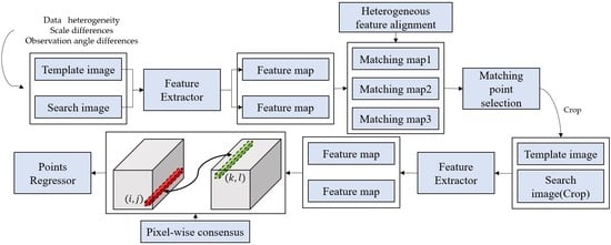
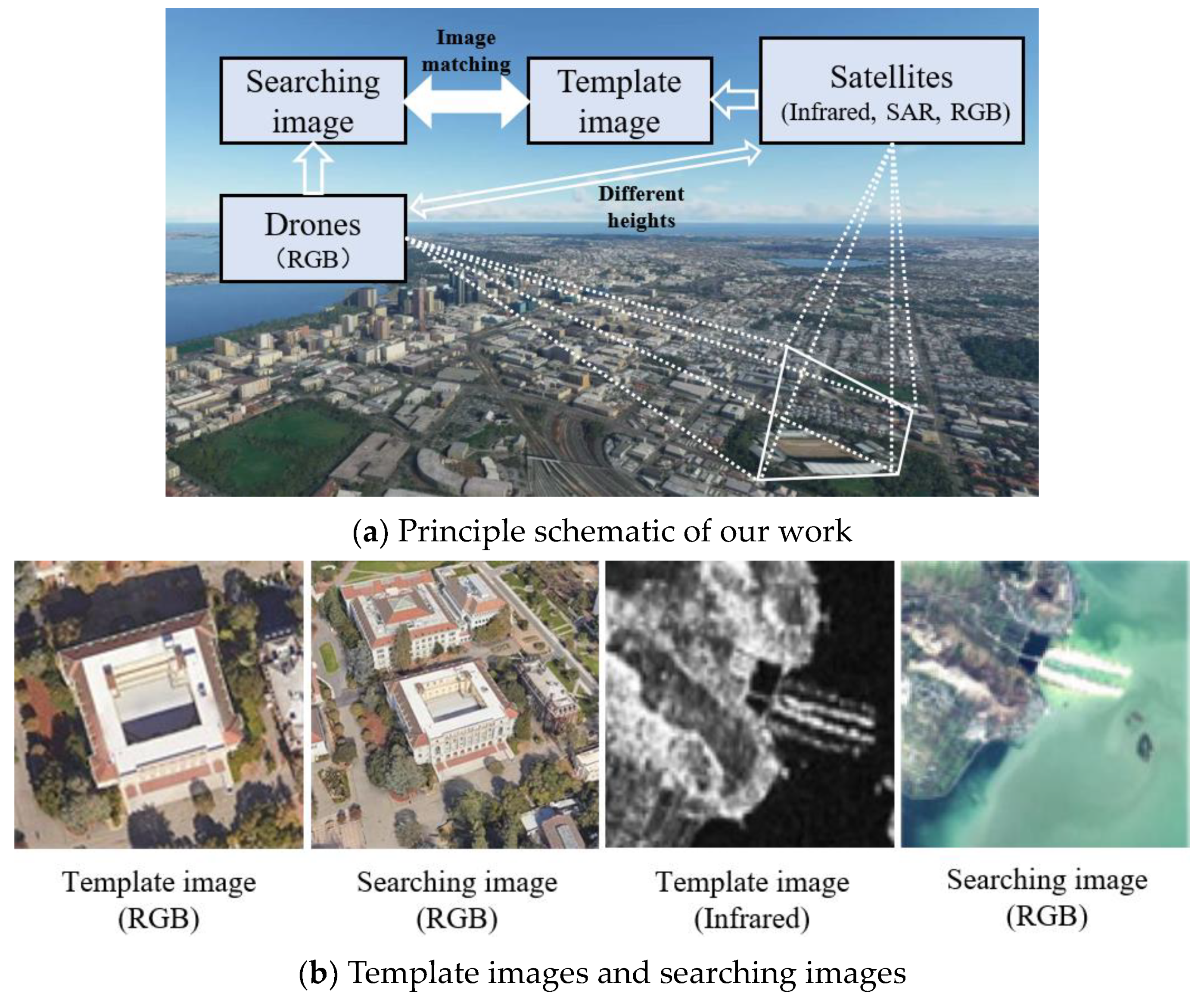
Data heterogeneity between template and search images;

(2)

Scale differences between template and search images;

(3)

Observation angle differences between template and search images.

Traditionally, visual correspondences consistent with geometric transformations, such as affine transformations, are processed using local features [2]. These features can be divided into point-based and region-based matching. Point-based matching uses feature points as local representations of image features, representing the original pixel intensities and being robust to luminance variations, affine variations, and noise. However, this method is only suitable for similar scenes with similar grayscale intensities, and performance will significantly decline when facing different image sources and views. Region-based matching [3,4,5] finds local features through feature descriptor similarity. Local features have good integrity and stability in cases of deformation and area change. However, this method lacks flexibility and adaptability when dealing with heterogeneous images and changes in viewpoint.

In recent years, deep neural networks (DNNs) have gradually been applied to remote sensing image processing. Due to their high flexibility and adaptiveness, DNNs have shown good performance in many tasks, such as semantic segmentation, change detection, and pixel-based classification [6,7,8]. In particular, the two-stream parallel network has become a common choice for many works [9]. Han et al. [10] proposed MatchNet, which segments the image into patches and then classifies them using the fully connected layer. Similarly, D2Net [11] and CMM-Net [12] segment the feature map to obtain feature descriptors and match points. The segmentation of images or feature maps, using the properties of a two-stream parallel network to calculate the similarity between two features, is a very effective method. However, there are some problems when faced with large-scale variations. Some researchers [13,14,15] proposed combining feature point extraction methods (SIFT [16], SURF [17]) with DCNN. These methods first use feature extraction operators to calculate possible match points and extract patches based on those points. Then, they use DCNN to calculate the similarity of the two patches, thus maintaining the correct and eliminating the incorrect points. The effectiveness and accuracy of these methods have been confirmed through numerous experiments. However, these methods are divided into two stages and cannot be trained as an end-to-end model. Rocco et al. [18] proposed a trainable model for affine transformation. They labeled the parameters and trained the model with the images in order to transform them. Furthermore, some works used DCNN to learn more reliable similarity metrics between descriptors, such as SuperPoint [19], SuperGlue [20], NCNet [21], and Patch2pix [22]. These models consider feature maps as feature descriptors and regress matching points by comparing the similarity between two feature maps. However, as in our work, remote sensing images often contain many complex and repeated textures, making it difficult to maintain accuracy against this background for pre-trained models based on point and edge datasets. On the other hand, images originate from different sensors (such as infrared, SAR, and RGB) and different platforms (such as satellite platforms and aviation platforms); hence, extracting and characterizing homologous features from heterogeneous features in multimodal images remains a challenge.

Considering the scale differences and viewpoint differences between the template image and the searching image, the object tracking methods are well suited to our work. Siamese neural network is the basic framework of object tracking methods. Broadly speaking, the two-stream parallel network is optimized and improved based on it and used for remote sensing image processing. Object trackers [23,24,25] usually use the first frame of a video as a template to track the next frame. Although the template has some deformation with the reference image of the next frame, this difference is slight. However, in our work, the templates were usually fixed and provided by a satellite, but the search view based on drones was constantly changing. This is a challenge for image matching, meaning that the trackers are not directly applicable to our work. Drawing lessons from the advantages of deep feature descriptors and object trackers, Zhang et al. [14] proposed a multi-modal remote sensing image matching method based on DNN. It was produced by a Siamese fully convolutional network, and a similarity score between two input images was obtained.

The abovementioned methods have been verified on different datasets. However, considering the heterogeneity of image features, scales and viewpoints in template matching tasks, an end-to-end trainable model is still required. In our work, we decomposed the template image matching of air- and space-based platforms into three main questions. The contributions of our work are as follows:

(1)

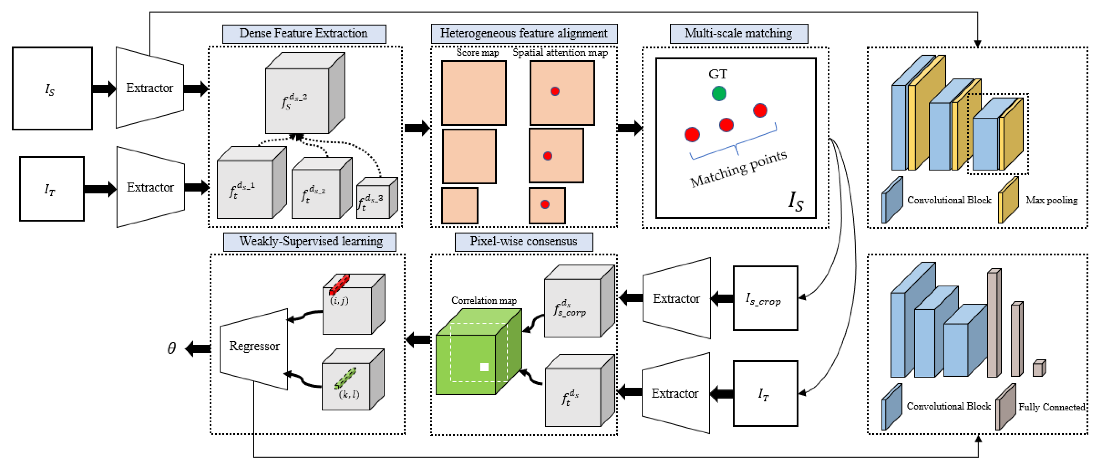
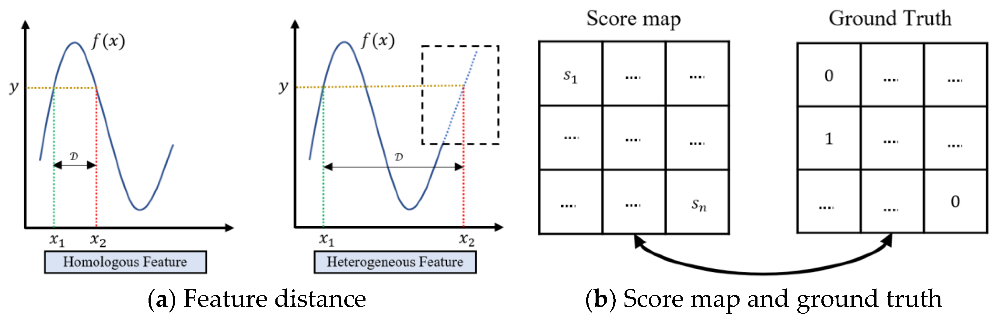
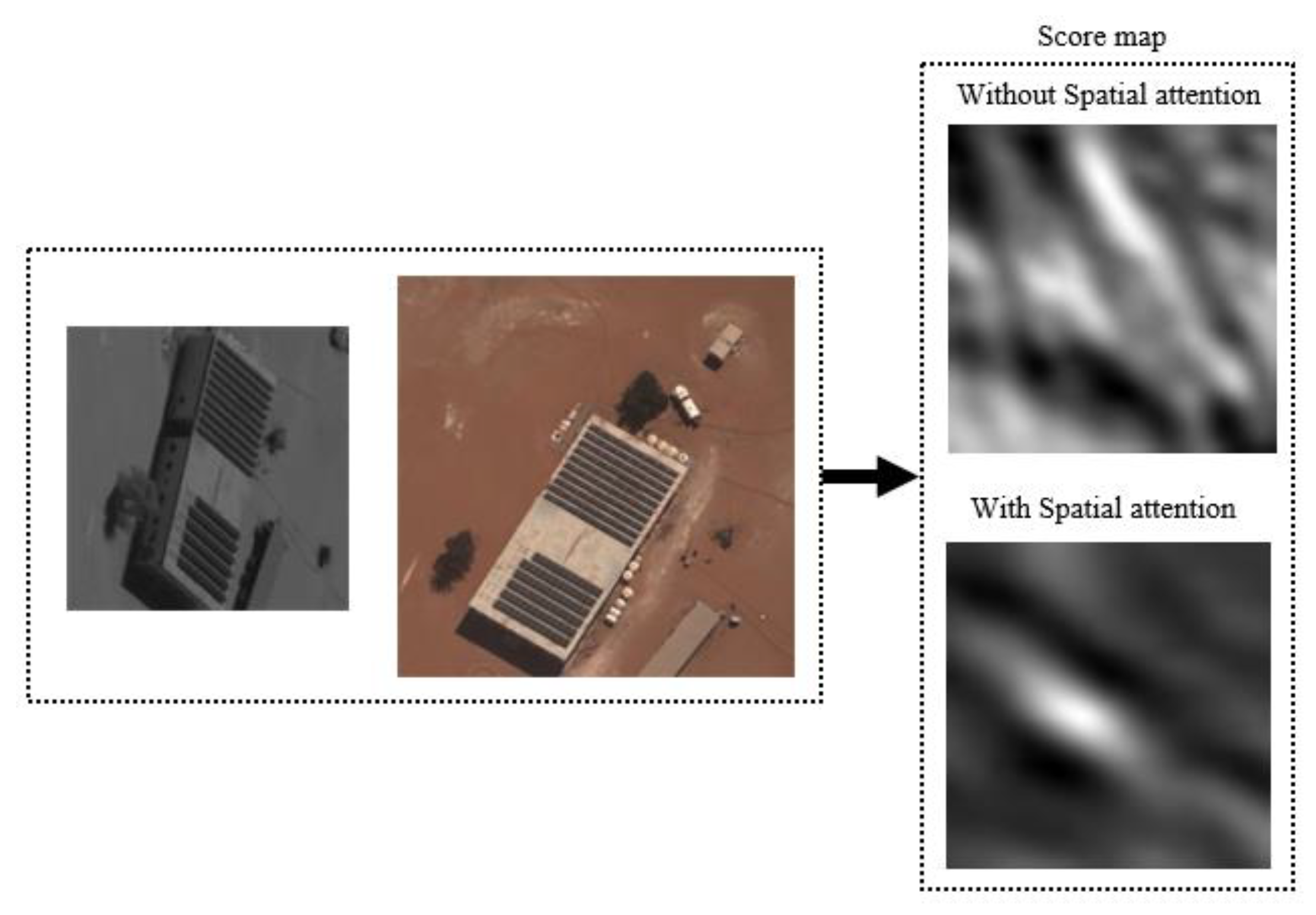
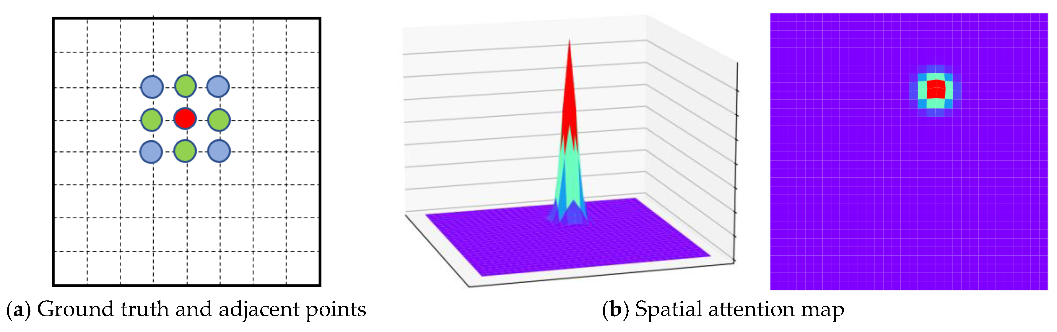
We propose a heterogeneous feature alignment method, aimed at addressing the problem of data heterogeneity between template and search images caused by sensor distances. Our approach utilizes the Siamese FC [23] as the main model for image matching and addresses domain shift issues by introducing a spatial attention map based on a 2D Gaussian distribution. This method forms an adaptive spatial activation using the 2D Gaussian distribution, which dynamically adjusts the weight of positive and negative samples in the loss function. This allows for convergence during training, reducing the distribution distance between heterogeneous features and enabling the model to better learn regional features for matching template and search images.

(2)

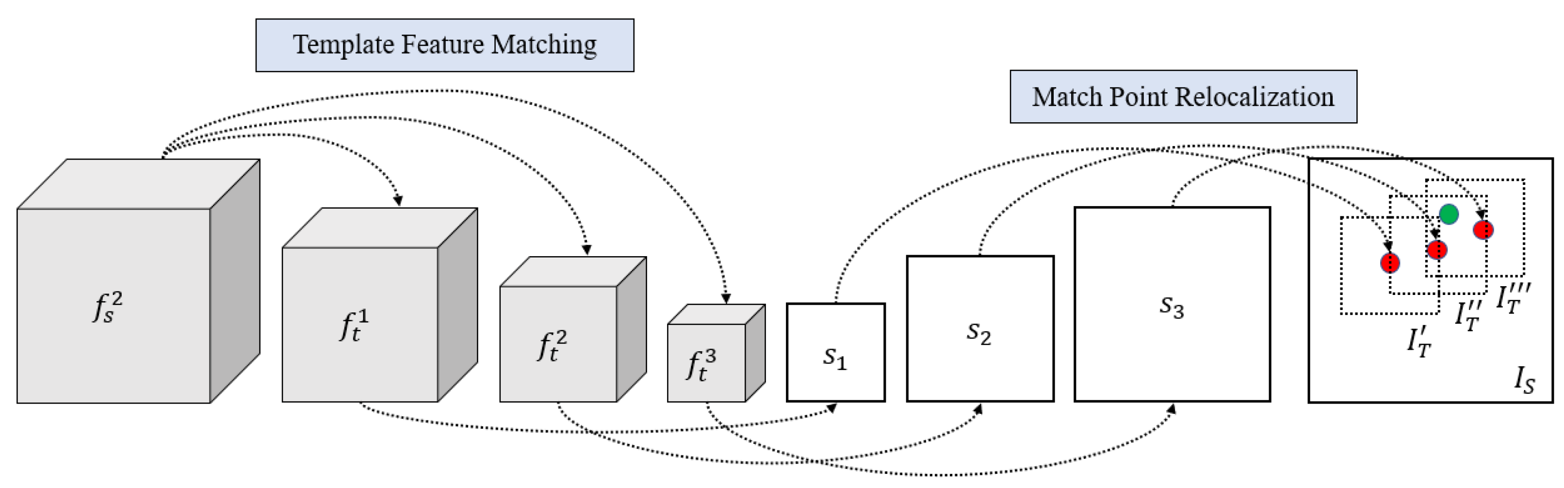
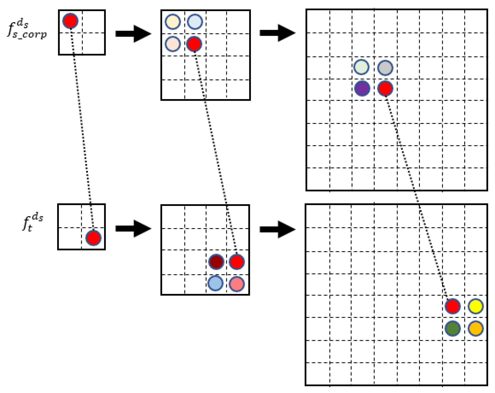
We propose a multi-scale matching method aimed at solving the problem of scale differences between search images and template images caused by observation distances. The template images provided by satellite are usually fixed, while the search images provided by aerial platforms vary with flight trajectories. Therefore, we propose a multi-scale matching method based on multi-level sub-sampling comparison. We extract feature maps of the template images at different sub-sampling levels of the model, respectively match them with the search images, obtain matching points, and determine the optimal matching points by comparing the Euclidean distance between each matching point and the ground truth.

(3)

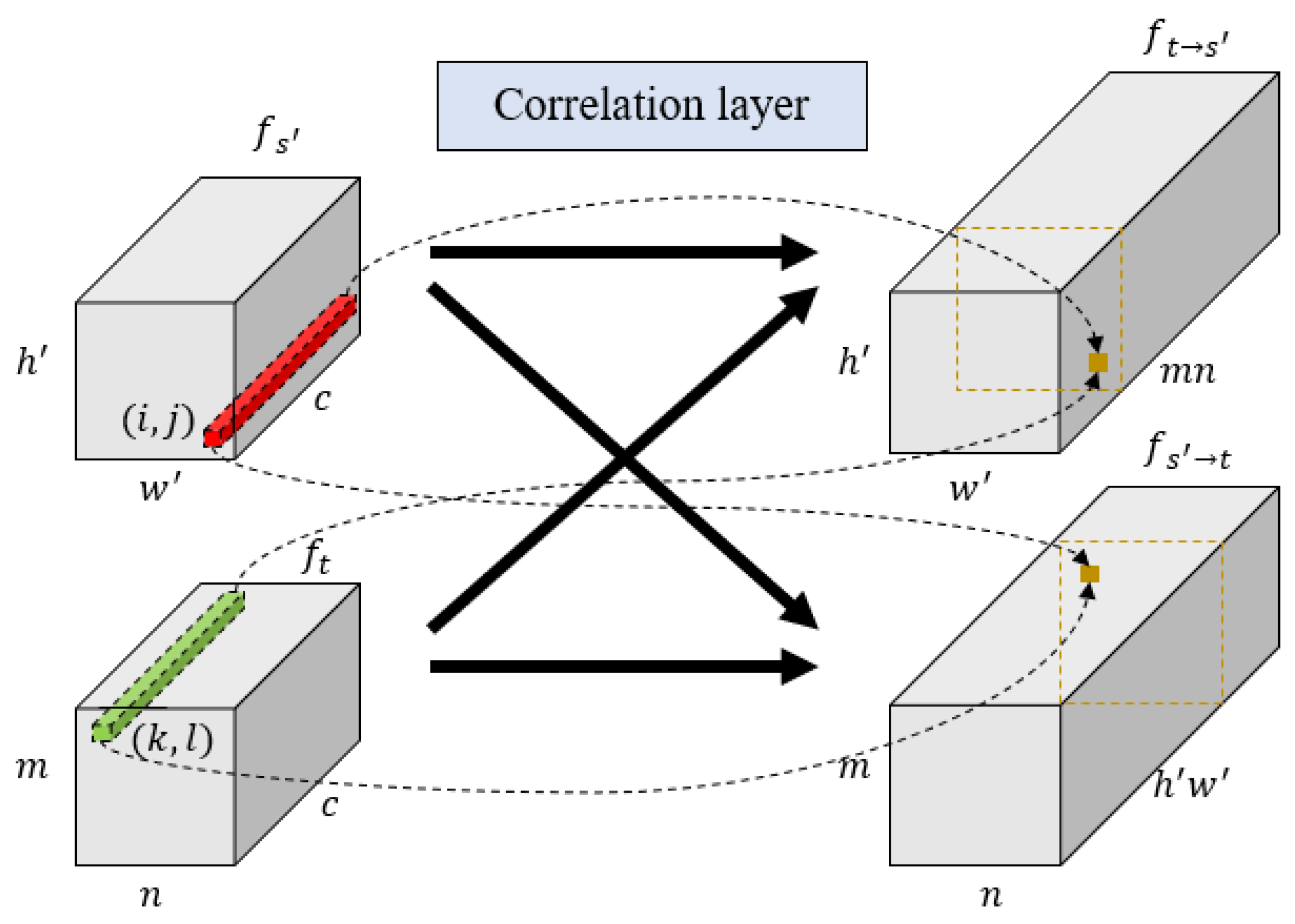
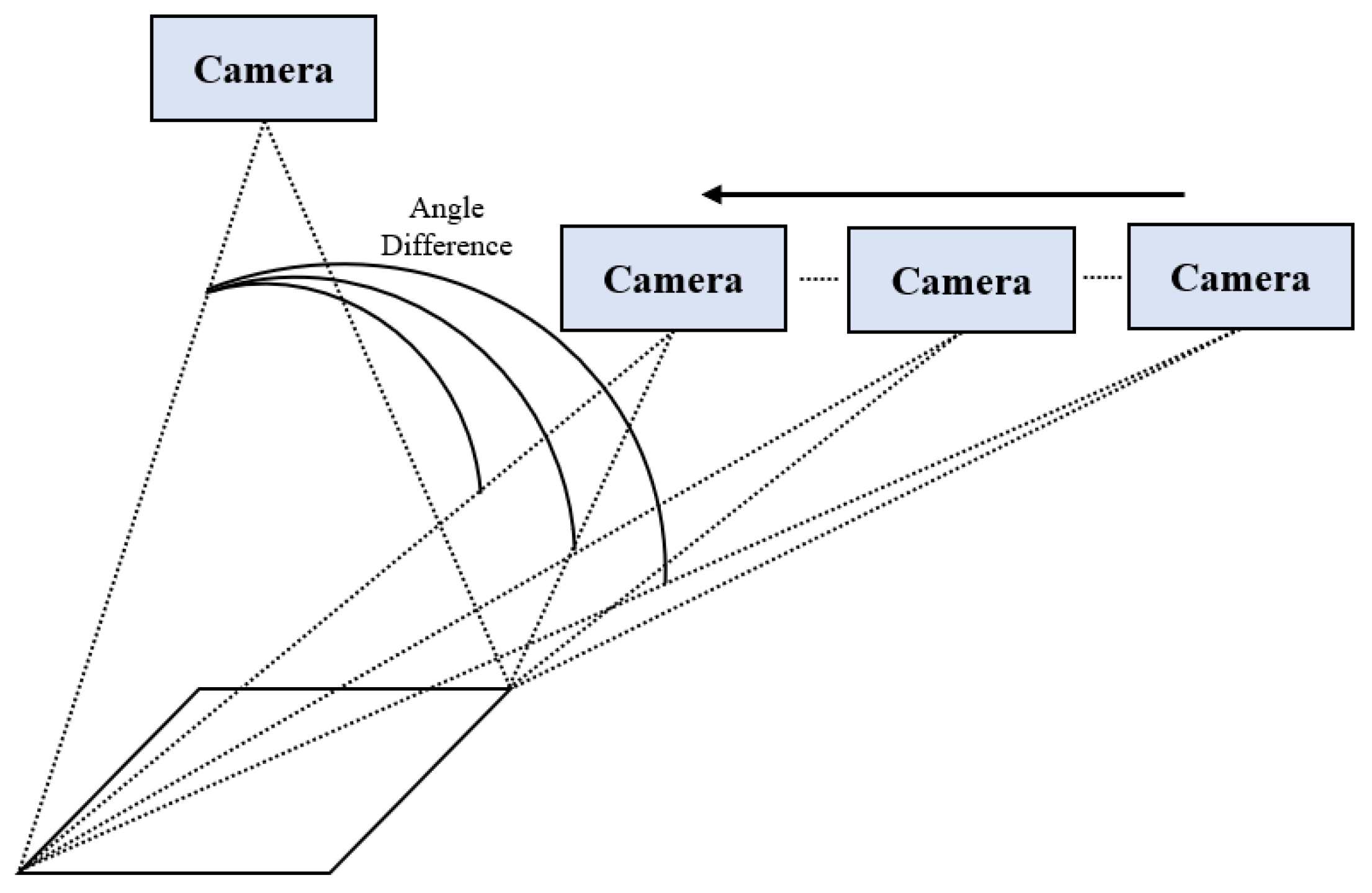
We proposed a pixel-wise consensus method aimed at addressing the problem of viewpoint differences between template and search images caused by different observation angles. After applying the two aforementioned methods, the model could determine the position of the template image in the search image and achieve image region-level matching. To further achieve image registration at different viewpoints, we proposed a pixel-wise consensus method based on a correlation layer. This method constructs a correlation map between the template feature map and the search feature map, and regresses the matching point pairs by solving for the points with the maximum correlation value.

(4)

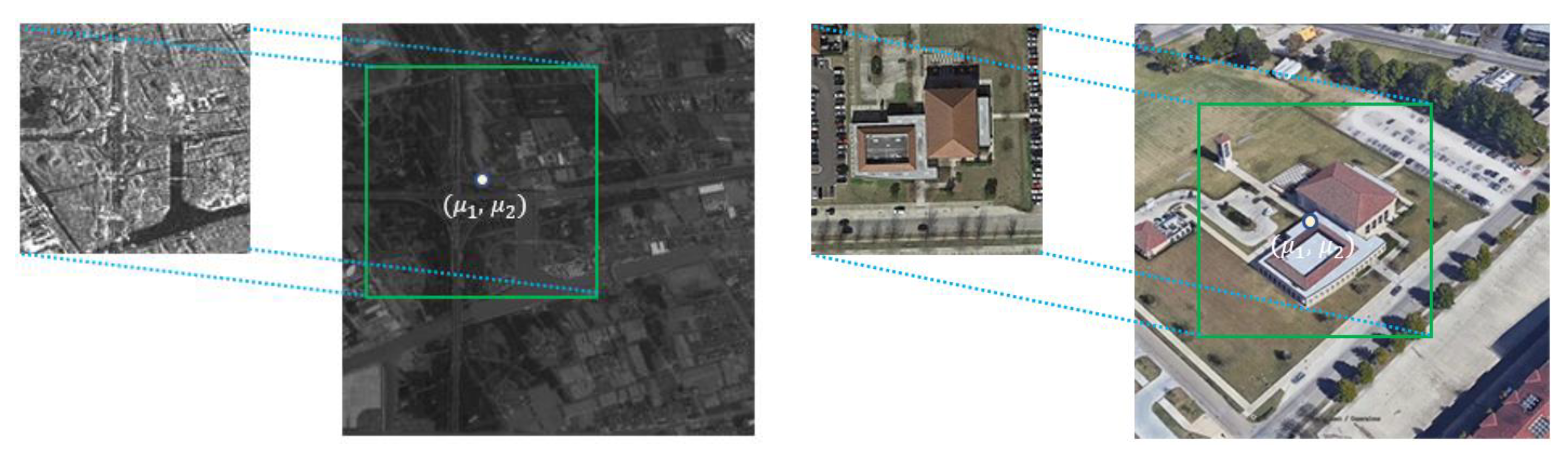
The annotation of labels for image matching is a labor-intensive and time-consuming task. Therefore, the weakly supervised learning method was proposed to reduce the labeling workload. In this method, we only labeled one point, which was the centroid of the template image, and indicated its position in the search image. The model could learn the local features during training and predict the location of the template image in the search image. We compared the distance between the ground truth and the prediction to determine the positive and negative samples, labeled as 1 and −1, respectively. Then, we implemented the regression process on the correlation map to produce pairs of matching points.

(5)

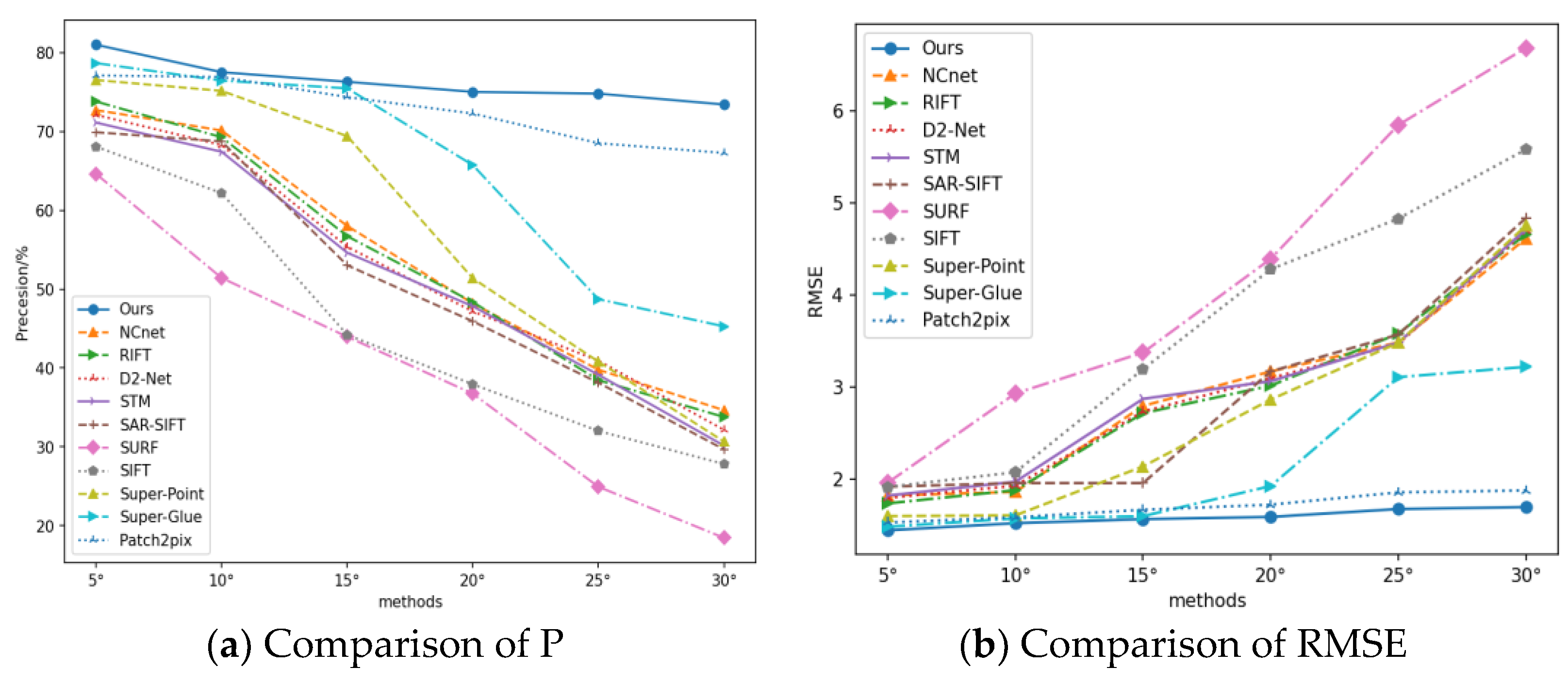
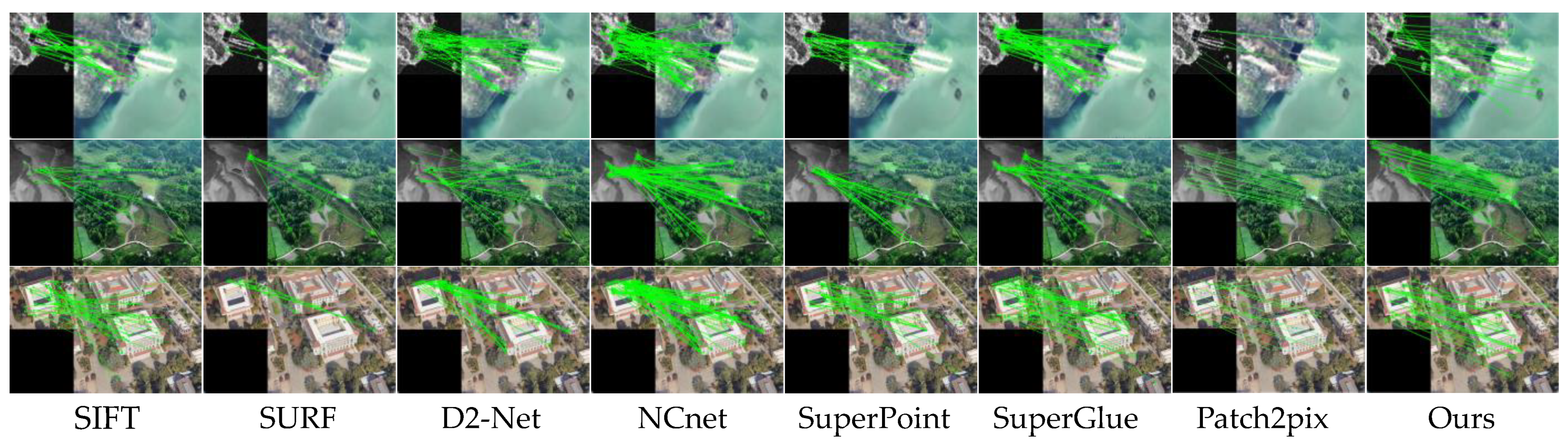
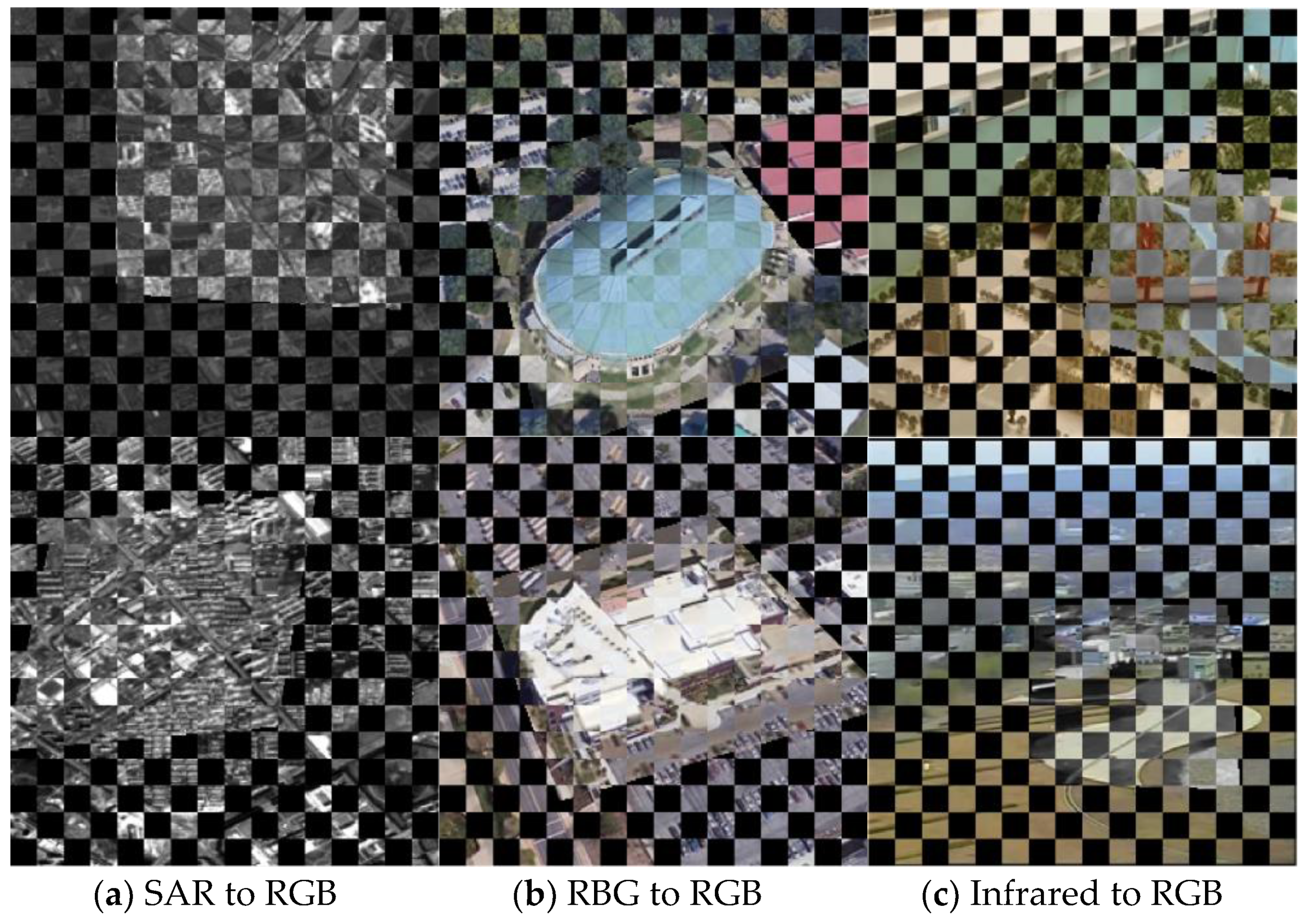
We conducted three types of matching experiments, including SAR to RGB, infrared to RGB, and RGB to RGB, each with viewpoint differences. Furthermore, to demonstrate the robustness of our method in the context of viewpoint changes, we conducted simulations at several exact angles. Additionally, we compared all of the experiments using different methods, including handcrafted and deep-learning-based methods, to verify the effectiveness of the proposed method and demonstrate its feasibility.

The remainder of this paper is structured as follows. Section 2 details the methods used for feature extraction, heterogeneous feature alignment, multi-scale matching, pixel-wise consensus, and weakly supervised learning. In Section 3, we present the experimental details, the dataset statement, and comparisons of the experimental results with several state-of-the-art methods, including ours. Finally, we provide conclusions in Section 4. An overview of our work is presented in Figure 2.

2. Methods

2.1. Dense Feature Extraction

Here, we follow the common practice of using CNN as a feature extractor, and the backbone of our method is a pre-trained VGG16 [26]. We consider the pre-trained model based on the open-source dataset to learn some edge and corner feature information, which is helpful for this task. We remove the full connection layer and retain the former 8 layers. Given the template image $I_T$ and the search image $I_S$, dense feature maps are produced by the feature extractor, and they can be formulated as:

$$f_s^d={\varphi }_1\left(I_S\right)$$

(1)

$$f_t^d={\varphi }_1\left(I_T\right)$$

(2)

where ${\varphi }_1$ denotes the feature extractor, and we consider the last layer of the feature extractor to be the activation maps. The spatial resolutions of the search image and template image are $\left(H,W\right)$ and $\left(M,N\right)$, respectively. Similarly, $\left(h,w\right)$ and $\left(m,n\right)$ denote the height and width of the search feature map $f_s^d$ and template feature map $f_t^d$, respectively. For the search image $I_S$, the spatial dimension of its feature map $f_s^d$ is $\frac{H}{2^{d }}$, where $d$ denotes the down-sampling operation. In our method, the number of down-samplings was set to 1, 2 and 3.

2.2. Heterogeneous Feature Alignment

The search feature map $f_s^d$ and template feature map $f_t^d$ contain the feature descriptions of the search image and template image. Many methods process these two feature maps directly. However, in our work, the template image was part of the search image, which means that the global information of the search image was redundant for pixel-wise registration. In order to further process the match points, we must first achieve the template feature matching to select the most relevant local information. Determining the most relevant area in the search image is a significant challenge. Usually, the template image obtained by satellite is RGB or SAR. As drones are often equipped with visible and infrared cameras, the search image is RGB. When the source sensors of the template image and search image are different, the problem of a domain gap arises. The same object has various features in different domains. For example, RGB images contain information on edge and color, but these types of data cannot be displayed in long-wave infrared images. (In our work, we used an infrared sensor with a wavelength of 8 μm, which is long-wave infrared and relatively lacking in edge information).

We followed the methods of previous object tracking works [26] and proposed the local area consensus network based on the Siamese network. Thus, $f_s^d\in {ℝ}^{h\times w\times c}$ and $f_t^d\in {ℝ}^{m\times n\times c}$ are processed through the convolutional operation, and then $f_t^d$ can be seen as a convolution kernel, which slides on $f_s^d$ to obtain the score map $s\in {ℝ}^{\left(h-m+1\right)\times \left(w-n+1\right)}$. Since the model structure is clear and fixed, the coordinates of each point on the score map correspond to the location of $f_t^d$ in $f_s^d$. We define the process in the following way:

$$s=Conv2d\left(f_t^d,f_s^d \right)$$

(3)

$$los{s}_{cla}=\frac{1}{n}{\displaystyle \sum }_n-\left[y_n·\log \left(s_n\right)+\left(1-y_n\right)·\log \left(1-s_n\right)\right]$$

(4)

where $s$ denotes the score map, which consists of predicted scores $s_n=\left(s_1,s_2,s_3\dots s_n\right)$, the convolutional stride is 1, and $y_n$ is the ground truth labelled by 0 and 1, as shown in Figure 3b.

Note that there is a problem of class imbalance, according to which we only have one positive sample but $\left(h-m+1\right)\left(w-n+1\right)-1$ as a negative sample. Ideally, the model will fit the position of the positive sample (labelled as 1). It is successful for images from the same source with the same viewpoint (as in object tracking, in which adjacent frames are used for processing). However, in our work, the template image and search image originated from different sources with different viewpoints. Clearly, the feature relevance was weaker, and the problem of class imbalance was amplified by the heterogeneous features, which prevented the model from converging during training, as shown in Figure 4.

In order to alleviate the domain gap, a feasible processing method is to diminish the high-level information distance of the template image and the search image. Let the coordinates of the score map be $\left(p_n,q_n\right)$. The spatial attention map is introduced based on a two-dimensional Gaussian distribution. This provides a solid incentive for the positive sample and weakens the redundant part of the global information. It also alleviates the domain gap and brings the heterogeneous features closer together in high-level features, which can be formulated as:

$$g\left(p_n,q_n\right)=\frac{1}{2\pi {\sigma }_1{\sigma }_2\sqrt{1-{\rho }^2}}{e}^{\left[-\frac{1}{2\left(1-{\rho }^2\right)}\left(\frac{{\left(p_n-{\mu }_1\right)}^2}{{\sigma }_1{}^2}-\frac{2\rho \left(p_n-{\mu }_1\right)+\left(q_n-{\mu }_2\right)}{{\sigma }_1{\sigma }_2}+\frac{{\left(q_n-{\mu }_2\right)}^2}{{\sigma }_2{}^2}\right)\right]}$$

(5)

where $\left({\mu }_1,{\mu }_2\right)$ is the location of the ground truth of the positive sample, the center point of the matching area (template image in search image). Here, ${\sigma }_1 \mathrm{and} {\sigma }_2$ determine the magnitude of the two-dimensional Gaussian distribution, which, intuitively, points adjacent to the ground truth by one pixel and, given an incentive, can facilitate the model fitting, as seen in Figure 5. Therefore, we set ${\sigma }_1, {\sigma }_2$ to 0.1. $\rho$ indicates the correlation coefficient. Since the pixels are independent, we set $\rho$ to 0. The two-dimensional Gaussian distribution can be simplified as follows:

$$g\left(p_n,q_n\right)=\frac{1}{2\pi {\sigma }_1{\sigma }_2 }{e}^{\left[-\frac{1}{2}\left(\frac{{\left(p_n-{\mu }_1\right)}^2}{{\sigma }_1}+\frac{{\left(q_n-{\mu }_2\right)}^2}{{\sigma }_2}\right)\right]}$$

(6)

During training, the spatial attention map dynamically adjusts the location of the incentive according to the ground truth on each matching scale and performs the calculation with the loss function:

$$los{s}_{cla}=\frac{1}{n}{\displaystyle \sum }_n-g\left(p_n,q_n\right)\left[y_n·\log \left(s_n\right)+\left(1-y_n\right)·\log \left(1-s_n\right)\right]$$

(7)

2.3. Multi-Scale Matching

The spatial resolution of the template image provided by the satellite is fixed, but the search area changes with the flight altitude of drones. Detectors [27,28] and trackers [24,25] usually use RPN and Anchor to accommodate object scale changes. However, in template matching, it is necessary to consider not only the features of the object itself but also the background information. Furthermore, our label only records the location of one pair of matching points; the size of the matching area does not participate in the regression calculation. Inspired by Yolo’s three-scale detection path, we introduced a multi-scale matching method to accommodate different flight altitudes. We applied the down-sampling times as different scale extraction standards. Then, three-scale template image feature maps of $f_t^d$ were obtained. After the convolutional operation, we could also obtain three-scale score maps, which can be defined as:

$$s_d=Conv2d\left(f_t^d,f_s^2\right)$$

(8)

The multi-scale matching process can be seen in Figure 6. In the training stage, three-scale template feature maps can cover different ranges in the search feature map, alleviating the problem of varying search horizons with different flight altitudes of drones. We constantly obtain three match points on the three-scale score maps by match point re-localization, and the model selects one score map for the loss calculation, which is determined by the Euclidean distance. The score map selection can be defined as:

$$\left(p^{\ast },q^{\ast }\right)=\underset{\left(p^d,q^d\right)}{\mathrm{argmin}}\sqrt{{\left(p^d-p^{gt}\right)}^2+{\left(q^d-q^{gt}\right)}^2},d=1, 2, 3$$

(9)

where $\left(p^{gt},q^{gt}\right)$ is the ground truth of the labelled points, $\left(p^d, q^d\right)$ denotes the inference points with the highest score of three scale, and $(p^{\ast }, q^{\ast })$ denotes the optimal inference points, which indicates the best score map.

2.4. Pixel-Wise Consensus

After the abovementioned processing, we obtained a certain area of the search image, which was highly correlated with the template image. To further achieve pixel-level registration, we introduced a correlation layer, which was first proposed in the study on FlowNet [29]. The correlation layer measures the similarity between two feature maps and does not need to be trained. Some researchers [18,21] have also used a correlation layer to achieve affine transformation and neighborhood consensus. In our work, we used the correlation layer to predict pairs of matching points, as shown in Figure 7. Assuming that we obtained a good match point $(p^{\ast }, q^{\ast })$ in $s_d$, we could then crop the search image $I_S$ to obtain $I_S^{crop}$. Let $d=2$, then the correlation feature map is:

$$f_{s^{\prime }}={\varphi }_1\left(I_S^{crop}\right)$$

(10)

$$f_t={\varphi }_1\left(I_T\right)$$

(11)

$$f_{t\to s^{\prime }}=\psi \left(f_{s^{\prime }},f_t\right)$$

(12)

$$f_{s^{\prime }\to t}=\psi \left(f_t,f_{s^{\prime }}, \right)$$

(13)

where $f_{s^{\prime }}$ denotes the feature map of the cropped search image. $\psi$ is the correlation layer, and $f_{t\to s^{\prime }}\in {ℝ}^{mn\times h^{\prime }\times w^{\prime }}$ is the template image dose for the correlation operation with the cropped search image. Correspondingly, $f_{s^{\prime }\to t}\in {ℝ}^{h^{\prime }{w}^{\prime }\times m\times n }$ is the cropped search image dose for the correlation operation with the template image. $f_{t\to s^{\prime }}$ and $f_{s^{\prime }\to t}$ are transpose relations, which contain all of the pairwise points.

Determining pairs of matching points, they can be defined as:

$$(i^{c_{k,l}},j^{c_{k,l}})=\underset{\left(i,j\right)}{\mathrm{argmax}}{f}_{t\to s^{\prime }}\left(c_{k,l},i,j \right), 1\le k\le m,1\le l\le n$$

(14)

$$(k^{c_{i,j}},l^{c_{i,j}})=\underset{\left(k,l\right)}{\mathrm{argmax}}{f}_{s^{\prime }\to t}\left(c_{i,j},k,l\right), 1\le i\le h^{\prime },1\le j\le w^{\prime }$$

(15)

$$c_{k,l}:=kn+l, c_{i,j}:=i{w}^{\prime }+j$$

(16)

$$k^{\ast }=\lfloor \frac{c_{k,l}}{m}\rfloor$$

(17)

$$l^{\ast }=c_{k,l}\mathit{mod}m$$

(18)

where $(k^{\ast },l^{\ast })$ denotes the point solved by $f_{t\to s^{\prime }}$. If $k^{\ast }=k \& l^{\ast }=l$, then $\left(i,j\right)$ and $\left(k,l\right)$ can be seen as pairs of matching points.

2.5. Weakly Supervised Learning

In this section, we define the weakly supervised training conducted in our work. Usually, fully supervised training is the preferred method, but in work such as ours, dense annotation consisting of pairs of points is time-consuming and complicated. Sparse annotation is one option, but it may cause imprecision. Therefore, it is desirable to propose a weakly supervised training method to train using a pair of images and to fit pairs of matching points. For this purpose, we proposed a training method that only needs one point in the annotation. Supposing the matching image $\left(I_T,I_S\right)$ and the matching feature map $\left(f_t^d,f_s^d\right)$, the $er$ can be obtained. The positive and negative can be defined as:

$$er=\sqrt{{\left(p^d-p^{gt}\right)}^2+{\left(q^d-q^{gt}\right)}^2}$$

(19)

$$Positive: \{\begin{array}{c}er\le 5, 0<epoch\le 50\\ er\le 2, 50<epoch\le 100\end{array}$$

(20)

$$Negative: \{\begin{array}{c}er>5, 0<epoch\le 50\\ er>2, 50<epoch\le 100\end{array}$$

(21)

where $epoch$ denotes the training epochs. Based on this definition, the $pos\left(f_{t\to s^{\prime }},f_{s^{\prime }\to t}\right)$ and $neg\left(f_{t\to s^{\prime }},f_{s^{\prime }\to t}\right)$ are obtained, and they are labelled as:

$$pos\left(f_{t\to s^{\prime }},f_{s^{\prime }\to t}\right)=1$$

(22)

$$neg\left(f_{t\to s^{\prime }},f_{s^{\prime }\to t}\right)=-1$$

(23)

From Section 2.4, we can obtain correlation feature maps $f_{t\to s^{\prime }}$ and $f_{s^{\prime }\to t}$. Due to their reciprocal transposition, we only choose one to form the regression. Ideally, the number of correct matching points of two perfectly matched images is $h^{\prime }\ast w^{\prime }$, but in the cross-view matching task, the number of matching points is much smaller than this value. Note that the size of the correlation map is $\left(mn,h^{\prime },w^{\prime }\right)$, which means that there is a significant amount of noise and a number of incorrect matching features. Therefore, we proposed the regression module ${\varphi }_2$, a cascade neural network consisting of a convolution layer and fully connected layer. First, considering the fact that the feature is available in the neighborhood of the correct point, we used the 1-kernel of the convolution layer to force the model to filter out redundant information and noise, each followed by Relu non-linearities. Through several layers, the channel dimension of the correlation map is reduced but maintains the spatial scale. Therefore, in this sparse tensor, a large amount of redundant information is filtered, while the stronger activated points are retained. The number of channel dimension reductions is set to $\frac{mn}{t}, t=2,4,6,8$. Then, the regression is processed based on $f_{t\to s^{\prime }}$ by the regression module ${\varphi }_2$:

$$\theta ={\varphi }_2\left(f_{t\to s^{\prime }}\right)$$

(24)

where ${\varphi }_2$ is a cascade neural network, and $\theta$ is the prediction. Additionally, the loss function can be defined, and it consists of two parts: the first is image region classification loss, illustrated in Section 2.2, Formula (7), and the second is match point regression loss. These parts can be defined as:

$$los{s}_{reg}=\frac{1}{M}{\displaystyle \sum }_{i=1}^M{\left(y_i-{\theta }_i\right)}^2$$

(25)

$$loss=los{s}_{cla}+los{s}_{reg}$$

(26)

2.6. Match Point Re-Localization

The area prediction was processed on the score map, and the match point regression was processed on the correlation map. Both were down-sampled during inference, and the pixel error was accumulated. In order to locate the exact location of the match points in the original resolution, we proposed a match point re-localization method.

Suppose that the cropped searching feature map $f_{s^{\prime }}$, and the template feature map $f_t$ and match points $\left(i,j,k,l\right)$ are obtained through Formulas (12)–(17). $f_{s^{\prime }}$ and $f_t$ are up-sampled by bilinear interpolation. Note that the maximum pooling size in our model is 2 ∗ 2; thus, each point corresponds to four points in the corresponding area of the up-sampled feature map. Furthermore, we use the cosine distance to compare the similarity between feature points. We first compare the most similar points in the up-sampled feature map; then, we confirm the most similar points between the two feature maps and proceed to the original resolution according to the down-sampling times. The processing stage is illustrated in Figure 8 and can be formulated as follows:

$$f_{s^{\prime }}{}^{\prime }=ℱ\left(f_{s^{\prime }}\right)$$

(27)

$$f_t{}^{\prime }=ℱ\left(f_t\right)$$

(28)

$$conf\left(f_{s^{\prime }},f_{s^{\prime }}{}^{\prime }\right)=ma{x}_{top-2}\left\{\frac{f_{ij}·f_{i_n{j}_n}}{\left|\right|f_{ij}{\left|\right|}_2\left|\right|f_{i_n{j}_n}{\left|\right|}_2}\right\}, \mathrm{n}=1,2,3,4$$

(29)

$$conf\left(f_t,f_t{}^{\prime }\right)=ma{x}_{top-2}\left\{\frac{f_{kl}·f_{k_n{l}_n}}{\left|\right|f_{kl}{\left|\right|}_2\left|\right|f_{k_n{l}_n}{\left|\right|}_2}\right\}, \mathrm{n}=1,2,3,4$$

(30)

$$\begin{array}{l}\mathit{conf}(f_t{}^{\prime },f_{s^{\prime }}{}^{\prime })\\ =\{\frac{f_{i^{\prime }{j}^{\prime }}·f_{k^{\prime }{l}^{\prime }}}{\left|\right|f_{i^{\prime }{j}^{\prime }}{\left|\right|}_2\left|\right|f_{k^{\prime }{l}^{\prime }}{\left|\right|}_2},\frac{f_{i^{″}{j}^{″}}·f_{k^{\prime }{l}^{\prime }}}{\left|\right|f_{i^{″}{j}^{″}}{\left|\right|}_2\left|\right|f_{k^{\prime }{l}^{\prime }}{\left|\right|}_2},\frac{f_{i^{\prime }{j}^{\prime }}·f_{k^{″}{l}^{″}}}{\left|\right|f_{i^{\prime }{j}^{\prime }}{\left|\right|}_2\left|\right|f_{k^{″}{l}^{″}}{\left|\right|}_2},\frac{f_{i^{″}{j}^{″}}·f_{k^{″}{l}^{″}}}{\left|\right|f_{i^{″}{j}^{″}}{\left|\right|}_2\left|\right|f_{k^{″}{l}^{″}}{\left|\right|}_2}\}\end{array}$$

(31)

where $ℱ$ is the bilinear interpolation, and $conf\left(f_{s^{\prime }},f_{s^{\prime }}{}^{\prime }\right)$ is the top-2 similarity between $f_{s^{\prime }}$ and the up-sampled feature map $f_{s^{\prime }}{}^{\prime }$, the same as $conf\left(f_t,f_t{}^{\prime }\right)$. Based on the confidence value, four candidate points can be obtained from each feature map, denoted as $\left(i^{\prime },j^{\prime }\right)$, $\left(i^{″},j^{″}\right)$, $\left(k^{\prime },l^{\prime }\right)$ $\left(k^{″},l^{″}\right)$. Then, the two $conf\left(f_t{}^{\prime },f_{s^{\prime }}{}^{\prime }\right)$ feature maps are obtained, indicating the match points in the up-sampled feature maps.

3. Experiments

3.1. Experimental Datasets

In this section, we present the details of three types of template matching experiments that we conducted to demonstrate the effectiveness and robustness of our proposed methods. The experiments were carried out as follows:

(1)

SAR to RGB: The SEN1-2 Dataset [30] was used for this part of the experiments. The dataset contained SAR images from Sentinel-1 satellites and multispectral images from Sentinel-2 satellites. The dataset included 32 cities and terrain such as mountains, forests, lakes, rivers, wastelands, buildings, etc., spanning a wide range of categories and thus being challenging for heterogeneous image matching. We cropped the SAR image as the template image and the RGB image as the search image. The total number of image pairs was 1200.

(2)

Infrared to RGB: The Drone-view, which is our self-built dataset, was used in this part of the experiments. We used the drone’s infrared and visible sensors to photograph the ground at 200 m and 500 m altitudes, respectively, as shown in Figure 9. The dataset contained a variety of scenarios, such as lakes, roads, mountains, etc. The images acquired at the 500 m altitude were template images, and the images acquired at the 200 m altitude were considered as search images. The total number of image pairs to conduct the experiment in this part was 3482.

(3)

RGB to RGB: The University-1652 [31] was used in this part of the experiments. This dataset contained maps of 1652 colleges and universities derived from three platforms: drones, satellites and ground cameras. We used the data of the drones and satellites, and the differences in viewpoints between the two was obvious. The images of the satellite were considered as direct template images, and the images of drones were regarded as search images. The total number of image pairs in this part of the evaluation was 701.

All image pairs were labelled, as shown in Figure 10. We moved the template image to the search image in order to find the matching area and label the center point coordinates. The coordinates can be imprecise due to the changing viewpoint; hence, we must specify the matching area. For the three types of template matching (SAR, infrared and RGB), the former (SAR) was the template image, and the last (RGB) was the search image. This process simulated the search view of the drones and the three types of templates provided by the satellites. The number of training sets and the test set were divided according to the ratio of 8:2, and the distribution used for each dataset is shown in

Table 1. Dataset distribution.

	Datasets	The SEN1-2 Dataset [30] (Contains Mountains, Cities, Lakes, Rivers, etc.)		The Drone-View (Contains Roads, Lakes, Rivers, etc.)		The University-1652 [31] (Contains Cities, Buildings, etc.)
Types		Training	Testing	Training	Testing	Training	Testing
SAR to RGB		960	240	N/A	N/A	N/A	N/A
Infrared to RGB		N/A	N/A	2786	696	N/A	N/A
RGB to RGB		N/A	N/A	N/A	N/A	561	140

. In our experiments, we used data augmentation to increase the size of the dataset, including random brightness, random grayscale, and adding Gaussian noise. During training, each augmentation strategy was applied once.

3.2. Experimental Details and Metrics

During training, 20% of the data was selected for testing, and 80% was selected for training with each dataset. We resized the search image to 512*512 and the template image to 128*128. The model parameters were optimized by SGD with a momentum of 0.9. The learning rate (LR) was set to 5 × 10⁻³ in the first 50 epochs and decayed every 50 epochs by 0.1 × 5 × 10⁻³. All of the experiments were implemented with an NVIDIA 2080Ti. In order to illustrate the effectiveness of our method, we compared both handcrafted and deep feature methods, including SIFT [16], SURF [17], D2-Net [11], NCnet [21], SuperPoint [19], SuperGlue [20], Patch2pix [22], RIFT [32], STM [33] and SAR-SIFT [34]. For the performance evaluation of the different methods, we introduced the Precision (P), Recall (R) and root-mean-square error (RMSE) to perform a quantitative analysis. They can be formulated as follows:

$$P=\frac{TP}{TP+FP}$$

(32)

$$R=\frac{TP}{TP+FN}$$

(33)

$$RMSE=\sqrt{\frac{1}{TP}{\displaystyle \sum }_{i=1}^{TP}{\left(x_i^{\prime }-x_i\right)}^2+{\left(y_i^{\prime }-x_i\right)}^2}$$

(34)

where $P$ is Precision and $R$ is Recall. TP, FN, FP and TN can be divided by the following rules:

• TP: Matching error ≤ 3 pixels.
• FN: Matching pairs ignored by the model.
• FP: Matching error > 3 pixels.
• TN: Remaining pixel pairs.

We also compared the inference times, counting the average time taken by each method to process a single image on the test set. In our experiments, the error rate of a point being less than 3 pixels was considered as the correct matching. In our work, we used the vectors of the coordinates where the matching pairs were located as feature descriptors. For each matching result, we could obtain a list of matching pairs, which could be recorded as $pairs=\left\{\left[\left[i_1,j_1\right],\left[k_1,l_1\right]\right],\dots .\left[\left[i_n,j_n\right],\left[k_n,l_n\right]\right]\right\}$. Furthermore, the vectors could be extracted as $pairs\_vec=\left\{\left[f_{ij}^1,f_{kl}^1\right],\dots \left[f_{ij}^n,f_{kl}^n\right]\right\}$. Therefore, the distance between feature descriptors could be defined as:

$$D\left(f_{ij},f_{kl}\right)=\left|\right|f_{ij}-f_{kl}{\left|\right|}_2$$

(35)

We sorted the distances and then used the 50th one as the threshold, and 50 matching pairs were obtained to calculate the image transfer parameters. Suppose that the matched pairs of feature points are $\left\{\left(x,y\right),\left(\tilde{x},\tilde{y}\right)\right\}$, and the transferred coordinates are $\left(x^{\prime },y^{\prime }\right)$, which originate from $\left(\tilde{x},\tilde{y}\right)$. $MA$ represents the proportion of correctly matched pairs, and RMSE indicates the deviation of $TP$ from the ground truth.

3.3. Experimental Results of SAR to RGB

From the results in

Table 2. Comparison of experimental results of SAR to RGB.

Methods	P	R	RMSE	Time
SIFT [16]	32.43%	31.28%	3.795	7.63 s
SURF [17]	33.47%	31.57%	3.783	2.40 s
SAR-SIFT [34]	39.73%	38.26%	3.658	4.48 s
STM [33]	43.77%	42.16%	3.364	0.95 s
D2Net [11]	62.16%	63.39%	2.393	1.62 s
RIFT [32]	64.81%	64.14%	2.327	5.32 s
NCnet [21]	74.02%	72.39%	1.824	0.82 s
SuperPoint [19]	72.48%	71.16%	1.867	0.12 s
SuperGlue [20]	76.14%	75.26%	1.761	0.14 s
Patch2pix [22]	78.68%	77.12%	1.603	0.76 s
Ours	81.49%	80.04%	1.528	0.09 s

, it can be seen that deep-learning-based methods have stronger adaptability and robustness compared to handcrafted methods in heterogeneous and complex scenarios. SIFT [16] and SURF [17] use pixel intensity for feature point matching; however, there are nonlinear intensity differences in heterogeneous images, and handcrafted algorithms are sensitive to such variations. They are not suitable for heterogeneous template matching.

Compared with handcrafted methods, deep-learning-based methods can extract high-level information depending on the intensity of the pixels, which provides the model with better adaptability. D2Net [11] and NCnet [21] extract a large number of feature points in terrain types such as harbors and rivers, but when faced with landscapes such as cities and mountains, the models extract many duplicate feature points. Because of the large number of duplicate textures in these types of terrain, these models are misleading. Relatively speaking, methods (SuperPoint [19], SuperGlue [20], Patch2pix [22] and ours) for determining feature points using image patches have better performance. Image patches provide more information than pixels, achieving a higher accuracy and robustness. Our method obtained 81.49%, 80.04% and 1.528 of P, R and RMSE, respectively. Compared with traditional methods (SIFT [16], SURF [17]), the metrics were increased by 49.06%, 48.76% and 2.267 and 48.02%, 48.47% and 2.255, respectively. On the other hand, our method has better performance than other deep learning methods. For example, compared with pixel-level methods (NCnet [21], SuperPoint [19] and SuperGlue [20]), we achieved a higher P, with results of 7.47%, 9.01% and 5.35%, respectively. The main reason for this phenomenon is that the model directly extracts feature points from global information. Thus, it is difficult for the model to determine the exact position of the template image in the search image when matching using feature points. Additionally, when the location of the template image shows deviation, the generation of feature points will also show deviation.

Relative to pixel-level methods, the RMSE values of patch–pixel-level methods (Patch2pix [22] and ours) are smaller, and the prediction deviation of feature points is less significant. They have better adaptability to viewpoint changes. Compared with Patch2pix [22], we achieved a higher P, R and RMSE of 2.81%, 2.92% and 0.075, respectively. Compared with multi-modal matching methods, such as RIFT [32] and SAR-SIFT [34], the P was increased by 16.68% and 41.76%, and the R was increased by 15.90% and 41.78%. SuperPoint [19], SuperGlue [20], and our method are the fastest-running methods. Compared to the former two methods, ours is approximately 0.05 s faster for inference. Our method has an advantage in regard to the template image location due to the heterogeneous feature alignment. Therefore, our method can extract more accurate feature points from the base mountain with precise template positioning. From the analysis of the abovementioned experimental results, including those of the deep methods and traditional methods, it can be seen that the template matching capability of the proposed method for SAR to RGB is better than that of the other methods.

3.4. Experimental Results of Infrared to RGB

The template image matching experiment was implemented on our own dataset. This dataset consisted of infrared and visible light data. We used a drone to shoot vertically at the altitude of 500 m for the template image and then took pictures at the altitude of 200 m with a 30° RGB axis, which was different from the vertical direction, as the search image, as shown in Figure 8.

Table 3. Comparison of experimental results for infrared to RGB.

Methods	P	R	RMSE	Time
SIFT [16]	44.79%	43.28%	3.228	7.71 s
SURF [17]	42.16%	42.03%	3.297	2.37 s
SAR-SIFT [34]	45.31%	46.21%	3.101	4.54 s
STM [33]	52.61%	51.47%	2.851	0.97 s
D2Net [11]	53.34%	52.71%	2.814	1.61 s
RIFT [32]	57.62%	55.18%	2.723	5.35 s
NCnet [21]	58.03%	57.83%	2.678	0.80 s
SuperPoint [19]	59.31%	59.12%	2.573	0.11 s
SuperGlue [20]	66.17%	65.44%	2.215	0.14 s
Patch2pix [22]	75.13%	74.67%	1.783	0.77 s
Ours	78.33%	77.14%	1.614	0.08 s

shows that the traditional methods obtained better performance in this experiment than SAR-to-RGB template matching. The main reason for this is that the background of our experimental site was a lake and shore, and the image background was relatively clean and straightforward.

However, for the pixel-level methods, the infrared to RGB matching performance was lower than that for SAR-to-RGB matching, because although the image background was simple, there were many repeated texture features, which led to erroneous matching. The patch–pixel-level methods are more suitable for this situation. Compared with Patch2pix [22], our method obtained 78.33%, 77.14% and 1.614 for P, R and RMSE and achieved higher values of 3.20%, 2.47% and 0.169 for P, R and RMSE, respectively. According to the above experimental analysis, whether SAR to RGB or infrared to RGB, the crucial aim is to achieve heterogeneous feature alignment. All of the methods captured low-level information; however, this is not enough for heterogeneous image template matching. Due to the spatial attention map, our method maintained good performance for heterogeneous feature alignment.

3.5. Experimental Results for RGB to RGB

From the results in

Table 4. Comparison of experimental results for RGB to RGB.

Methods	P	R	RMSE	Time
SIFT [16]	64.16%	65.43%	1.924	7.36 s
SURF [17]	61.47%	60.18%	2.416	2.32 s
SAR-SIFT [34]	67.42%	68.79%	1.902	4.52 s
STM [33]	72.02%	71.68%	1.887	0.96 s
D2Net [11]	73.67%	73.28%	1.761	1.58 s
RIFT [32]	74.48%	74.16%	1.748	5.32 s
NCnet [21]	75.93%	76.17%	1.682	0.78 s
SuperPoint [19]	78.41%	77.84%	1.603	0.13 s
SuperGlue [20]	81.29%	80.16%	1.519	0.13 s
Patch2pix [22]	83.48%	83.73%	1.451	0.76 s
Ours	85.16%	86.32%	1.397	0.09 s

, it can be seen that all of the methods obtained better performance than those described in Section 3.3 and Section 3.4. The main reason for this phenomenon is that the template image and the search image were homologous. There was little difference between handcrafted and deep-learning-based methods in homologous image matching because the homologous images had similar pixel intensities in the matched feature points. However, the experiments still reflected the methods’ resistance capability for viewpoint change. Our method obtained 85.16%, 86.32% and 1.397 for P, R and RMSE, respectively. Compared with SuperGlue [20] and Patch2pix [22], we achieved higher values of 3.87% and 1.68% for P, respectively. On the other hand, the traditional method, SIFT [16], which does not involve training, obtained 64.16% and 65.43% for P and R, being approximately 10% lower than the values for the deep learning methods.

Compared with the previous experiments, this shows that the deep learning methods have more advantages in more complex situations, such as repeated textures, complicated image backgrounds and heterogeneous images. This requires that the model extract high-level information about feature points to avoid errors. From the above analysis, although there was no apparent gap between the methods in terms of performance, it still can be seen that our method had higher performance in RGB-to-RGB template matching due to the cross-viewpoint matching method of the pixel-wise consensus method.

3.6. Experimental Results for Different Viewpoints

In the previous experiments, we evaluated the performance of our method on each of the three datasets. However, it was unclear how well the model performed at specific viewing angles. Therefore, we conducted an additional experiment on the infrared to RGB dataset to simulate a range of angular differences using both a fixed camera and a movable camera to mimic space-based observations. The process is illustrated in Figure 9.

As shown in

Table 5. Comparison of experimental results for different viewpoints.

	Methods	SIFT [16]	SURF [17]	SAR-SIFT [34]	STM [33]	D2-Net [11]	RIFT [32]	NCnet [21]	SuperPoint [19]	SuperGlue [20]	Patch2pix [22]	Ours
Angle/Metrics
5°	P	68.08%	64.62%	69.91%	71.13%	72.11%	73.81%	72.72%	76.53%	78.68%	77.12%	81.01%
	R	67.52%	63.18%	68.82%	70.16%	71.68%	72.93%	71.67%	75.83%	77.15%	76.88%	80.57%
	RMSE	1.911	1.957	1.914	1.817	1.792	1.732	1.818	1.594	1.478	1.524	1.439
10°	P	62.17%	51.42%	68.74%	67.43%	68.28%	69.27%	70.13%	75.16%	76.46%	76.92%	77.53%
	R	61.72%	50.73%	67.93%	66.81%	67.65%	68.12%	69.65%	74.83%	75.93%	75.36%	76.57%
	RMSE	2.071	2.928	1.953	1.968	1.924	1.876	1.857	1.602	1.569	1.581	1.517
15°	P	44.21%	43.96%	53.03%	54.62%	55.38%	56.72%	58.02%	69.41%	75.48%	74.37%	76.31%
	R	43.82%	43.15%	53.67%	53.73%	54.91%	56.87%	57.68%	68.16%	74.37%	73.68%	75.29%
	RMSE	3.191	3.372	2.984	2.869	2.731	2.713	2.792	2.134	1.593	1.663	1.561
20°	P	37.93%	36.74%	45.92%	47.83%	47.17%	48.36%	48.18%	51.37%	65.74%	72.28%	75.03%
	R	36.58%	35.73%	44.78%	46.37%	46.82%	49.21%	47.62%	50.19%	64.43%	71.37%	74.62%
	RMSE	4.278	4.391	3.167	3.061	3.093	3.012	3.167	2.861	1.921	1.718	1.585
25°	P	32.01%	24.93%	38.13%	39.14%	40.93%	38.46%	39.78%	40.81%	48.73%	68.52%	74.81%
	R	32.14%	23.69%	37.82%	38.76%	39.63%	37.53%	38.64%	39.73%	47.92%	67.68%	73.64%
	RMSE	4.829	5.847	3.568	3.481	3.468	3.578	3.483	3.479	3.105	1.852	1.671
30°	P	27.82%	18.45%	29.68%	30.15%	32.15%	33.78%	34.64%	30.67%	45.28%	67.28%	73.43%
	R	26.82%	17.67%	28.52%	29.27%	31.76%	32.41%	33.71%	29.68%	44.62%	66.69%	72.57%
	RMSE	5.581	6.686	4.836	4.712	4.696	4.659	4.613	4.752	3.217	1.873	1.692

, we conducted experiments for six angles increasing every 5°, and the maximum angle difference was 30°. In each angle experiment, our method obtained the best performance. In the experiments with a slight angle difference, such as 5° and 10°, the performance of the different methods was not clear. Our method achieved higher values of 3.89% and 2.33% for P than Patch2pix [22] and Super-Glue [20], and the performance of the traditional methods was very close to some deep learning methods. However, in the experiments with a large angle difference, our proposed method demonstrated stability and robustness. In particular, in the experiments with 25° and 30° angle differences, our method obtained 74.81% and 73.43% for P and 73.64% and 72.57% for R, respectively, while the performance of the remaining methods was severely degraded. It can be seen from Figure 11 that our method had the least performance degradation as the angle difference increased, which demonstrates the better robustness and adaptability of our proposed method. Some matching results can be seen in Figure 12, which shows the matching effects of different methods on SAR to RGB, Infrared to RGB, and RGB to RGB. We visualized the checkerboard mosaic for each of the three matching types, and the results are shown in Figure 13. From the results in the figure, we can see that the template image effectively covered the corresponding region in the search image, indicating that our method rendered a template image highly suitable for the matching of the correct position.

4. Conclusions

In this work, we proposed a novel method for cross-view heterogeneous template matching that can be applied to both air- and space-based platforms. However, due to the inherent differences in their working environments and payloads, we faced three significant challenges that needed to be addressed. Firstly, the images produced by different sensors were heterogeneous. Secondly, we observed scale variations caused by different heights. Lastly, feature distortion was caused by different viewing angles. To tackle these issues, we proposed the following methods:

(1)

To address the first challenge of the heterogeneous images produced by different sensors, we proposed a method called the heterogeneous feature alignment method based on the spatial attention map. In this approach, we added a two-dimensional Gaussian distribution to the loss function to minimize the distance between the distributed heterogeneous features. By doing so, we can effectively match the features of the template image with those of the search image, allowing them to correspond to each other.

(2)

To address the second challenge of the scale variation caused by different heights, we proposed a multi-scale matching method based on multi-layer sampling point regression. With this approach, we perform regression on the matching points at different down-sampling scales to preserve the result with the smallest distance error. By doing so, we can effectively match the template and search images at different scales, overcoming the challenge of scale variation caused by different heights.

(3)

To address the third challenge of feature distortion caused by different viewing angles, we proposed a pixel-wise consensus method based on the correlation layer. With this method, we use a correlation layer to extract the pixel points with the highest correlation between the feature maps of the search image and the template image, thus obtaining the matching feature points. By doing so, we can effectively overcome the feature distortion caused by different viewing angles and achieve accurate template matching.

Furthermore, considering the complexity and time-consuming nature of annotation, we proposed a weakly supervised learning method to minimize the annotation efforts required. With this method, we only need to label one point to indicate the location of the template image in the search image, thereby completing the entire training process. Four parts of the experiment demonstrated the robustness and effectiveness of our proposed methods. In the experiment on different viewpoints, our method showed good adaptability to changes in viewpoint and maintained a high level of accuracy. Specifically, when the maximum viewpoint difference was 30 degrees, our method achieved a precision of 73.43%, a recall of 72.57%, and an RMSE of 1.692. These results demonstrate that our proposed method is well-suited for cross-view heterogeneous template matching with air- and space-based platforms.

References

1. Sattler, T.; Maddern, W.; Toft, C.; Torii, A.; Hammarstrand, L.; Stenborg, E.; Safari, D.; Okutomi, M.; Pollefeys, M.; Sivic, J.; et al. Benchmarking 6DOF Outdoor Visual Localization in Changing Conditions. In Proceedings of the 2018 IEEE/CVF Conference on Computer Vision and Pattern Recognition, Salt Lake City, UT, USA, 18–23 June 2018; pp. 8601–8610. [Google Scholar] [CrossRef]
2. Taira, H.; Okutomi, M.; Sattler, T.; Cimpoi, M.; Pollefeys, M.; Sivic, J.; Pajdla, T.; Torii, A. InLoc: Indoor Visual Localization with Dense Matching and View Synthesis. IEEE Trans. Pattern Anal. Mach. Intell. 2019, 43, 1293–1307. [Google Scholar] [CrossRef] [PubMed]
3. Dalal, N.; Triggs, B. Histograms of oriented gradients for human detection. In Proceedings of the 2005 IEEE Computer Society Conference on Computer Vision and Pattern Recognition, San Diego, CA, USA, 20–25 June 2005; pp. 886–893. [Google Scholar] [CrossRef]
4. Ham, B.; Cho, M.; Schmid, C.; Ponce, J. Proposal Flow. In Proceedings of the 2016 IEEE Conference on Computer Vision and Pattern Recognition, Las Vegas, NV, USA, 27–30 June 2016; pp. 3475–3484. [Google Scholar] [CrossRef]
5. Lowe, D.G. Distinctive Image Features from Scale-Invariant Keypoints. Int. J. Comput. Vis. 2004, 60, 91–110. [Google Scholar] [CrossRef]
6. Zhao, Z.; Jiao, L.; Zhao, J.; Gu, J.; Zhao, J. Discriminant deep belief network for high-resolution SAR image classification. Pattern Recognit. 2017, 61, 686–701. [Google Scholar] [CrossRef]
7. Alali, F.M.; Tarakji, B.; Alqahtani, A.S.; Alqhtani, N.R.; Nabhan, A.B.; Alenzi, A.; Alrafedah, A.; Robaian, A.; Noushad, M.; Kujan, O.; et al. SAR Image segmentation based on convolutional-wavelet neural network and markov random field. Pattern Recognit. 2017, 64, 255–267. [Google Scholar] [CrossRef]
8. Zhao, W.; Jiao, L.; Ma, W.; Zhao, J.; Zhao, J.; Liu, H.; Cao, X.; Yang, S. Superpixel-Based Multiple Local CNN for Panchromatic and Multispectral Image Classification. IEEE Trans. Geosci. Remote Sens. 2017, 55, 4141–4156. [Google Scholar] [CrossRef]
9. Altwaijry, H.; Trulls, E.; Hays, J.; Fua, P.; Belongie, S. Learning to Match Aerial Images with Deep Attentive Architectures. In Proceedings of the 2016 IEEE Conference on Computer Vision and Pattern Recognition, Las Vegas, NV, USA, 27–30 June 2016; pp. 3539–3547. [Google Scholar] [CrossRef]
10. Han, X.; Leung, T.; Jia, Y.; Sukthankar, R.; Berg, A.C. Matchnet: Unifying feature and metric learning for patch-based matching. In Proceedings of the IEEE Conference on Computer Vision and Pattern Recognition, Boston, MA, USA, 7–12 June 2015; pp. 3279–3286. [Google Scholar] [CrossRef]
11. Dusmanu, M.; Rocco, I.; Pajdla, T.; Pollefeys, M.; Sivic, J.; Torii, A.; Sattler, T. D2-Net: A Trainable CNN for Joint Description and Detection of Local Features. In Proceedings of the 2019 IEEE/CVF Conference on Computer Vision and Pattern Recognition, Long Beach, CA, USA, 15–20 June 2019; pp. 8084–8093. [Google Scholar] [CrossRef]
12. Cui, S.; Ma, A.; Wan, Y.; Zhong, Y.; Luo, B.; Xu, M. Cross-Modality Image Matching Network with Modality-Invariant Feature Representation for Airborne-Ground Thermal Infrared and Visible Datasets. IEEE Trans. Geosci. Remote Sens. 2022, 60, 1–14. [Google Scholar] [CrossRef]
13. Zhu, H.; Jiao, L.; Ma, W.; Liu, F.; Zhao, W. A Novel Neural Network for Remote Sensing Image Matching. IEEE Trans. Neural Netw. Learn. Syst. 2019, 30, 2853–2865. [Google Scholar] [CrossRef] [PubMed]
14. Zhang, H.; Ni, W.; Yan, W.; Xiang, D.; Wu, J.; Yang, X.; Bian, H. Registration of Multi-modal Remote Sensing Image Based on Deep Fully Convolutional Neural Network. IEEE J. Sel. Top. Appl. Earth Obs. Remote Sens. 2019, 12, 3028–3042. [Google Scholar] [CrossRef]
15. Li, Z.; Zhang, H.; Huang, Y. A Rotation-Invariant Optical and SAR Image Registration Algorithm Based on Deep and Gaussian Features. Remote Sens. 2021, 13, 2628. [Google Scholar] [CrossRef]
16. Lowe, D.G. Object recognition from local scale-invariant features. In Proceedings of the Seventh IEEE International Conference on Computer Vision, Kerkyra, Greece, 20–27 September 1999; Volume 2, pp. 1150–1157. [Google Scholar] [CrossRef]
17. Bay, H.; Tuytelaars, T. Van Gool, LSurf: Speeded up robust features. In Computer Vision—ECCV 2006, Proceedings of the 9th European Conference on Computer Vision, Graz, Austria, 7–13 May 2006; Springer: Berlin/Heidelberg, Germany, 2006; pp. 404–417. [Google Scholar] [CrossRef]
18. Rocco, I.; Arandjelovic, R.; Sivic, J. Convolutional Neural Network Architecture for Geometric Matching. In Proceedings of the 2017 IEEE Conference on Computer Vision and Pattern Recognition, Honolulu, HI, USA, 21–26 July 2017; pp. 39–48. [Google Scholar] [CrossRef]
19. DeTone, D.; Malisiewicz, T.; Rabinovich, A. SuperPoint: Self-Supervised Interest Point Detection and Description. In Proceedings of the 2018 IEEE/CVF Conference on Computer Vision and Pattern Recognition Workshops, Salt Lake City, UT, USA, 18–22 June 2018; pp. 337–350. [Google Scholar] [CrossRef]
20. Sarlin, P.E.; DeTone, D.; Malisiewicz, T.; Rabinovich, A. SuperGlue: Learning Feature Matching with Graph Neural Networks. In Proceedings of the 2020 IEEE/CVF Conference on Computer Vision and Pattern Recognition, Seattle, WA, USA, 13–19 June 2020; pp. 4937–4946. [Google Scholar] [CrossRef]
21. Rocco, I.; Cimpoi, M.; Arandjelović, R.; Torii, A.; Pajdla, T.; Sivic, J. NCNet: Neighbourhood Consensus Networks for Estimating Image Correspondences. IEEE Trans. Pattern Anal. Mach. Intell. 2022, 44, 1020–1034. [Google Scholar] [CrossRef]
22. Zhou, Q.; Sattler, T.; Leal-Taixé, L. Patch2Pix: Epipolar-Guided Pixel-Level Correspondences. In Proceedings of the 2021 IEEE/CVF Conference on Computer Vision and Pattern Recognition, Nashville, TN, USA, 20–25 June 2021; pp. 4667–4676. [Google Scholar] [CrossRef]
23. Bertinetto, L.; Valmadre, J.; Henriques, J.F.; Vedaldi, A.; Torr, P.H.S. Fully-Convolutional Siamese Networks for Object Tracking. In Computer Vision—ECCV 2016 Workshops. ECCV 2016; Springer: Cham, Switzerland, 2016; pp. 850–865. [Google Scholar] [CrossRef]
24. Li, B.; Yan, J.; Wu, W.; Zhu, Z.; Hu, X. High Performance Visual Tracking with Siamese Region Proposal Network. In Proceedings of the 2018 IEEE/CVF Conference on Computer Vision and Pattern Recognition, Salt Lake City, UT, USA, 18–23 June 2018; pp. 8971–8980. [Google Scholar] [CrossRef]
25. Li, B.; Wu, W.; Wang, Q.; Zhang, F.; Xing, J.; Yan, J. SiamRPN++: Evolution of Siamese Visual Tracking with Very Deep Networks. In Proceedings of the 2019 IEEE/CVF Conference on Computer Vision and Pattern Recognition, Long Beach, CA, USA, 15–20 June 2019; pp. 4277–4286. [Google Scholar] [CrossRef]
26. Simonyan, K.; Zisserman, A. Very Deep Convolutional Networks for Large-Scale Image Recognition. 2014. Available online: https://arxiv.org/abs/1409.1556 (accessed on 1 October 2021).
27. Bochkovskiy, A.; Wang, C.; Liao, H. YOLOv4: Optimal Speed and Accuracy of Object Detection. arXiv 2020, arXiv:2004.10934. [Google Scholar]
28. Ge, Z.; Liu, S.; Wang, F.; Li, Z.; Sun, J. YOLOX: Exceeding YOLO Series in 2021. arXiv 2021, arXiv:2107.08430. [Google Scholar]
29. Dosovitskiy, A.; Fischer, P.; Ilg, E.; Hausser, P.; Hazirbas, C.; Golkov, V.; Van Der Smagt, P.; Cremers, D.; Brox, T. FlowNet: Learning Optical Flow with Convolutional Networks. In Proceedings of the 2015 IEEE International Conference on Computer Vision, Santiago, Chile, 7–13 December 2015; pp. 2758–2766. [Google Scholar] [CrossRef]
30. Schmitt, M.; Hughes, L.H.; Zhu, X. The SEN1-2 Dataset for Deep Learning in SAR-RGB Data Fusion. arXiv 2018, arXiv:1807.01569. [Google Scholar]
31. Zheng, Z.; Wei, Y.; Yang, Y. University-1652: A Multi-view Multi-source Benchmark for Drone-based Geo-localization. arXiv 2020, arXiv:2002.12186. [Google Scholar]
32. Li, J.; Hu, Q.; Ai, M. RIFT: Multi-Modal Image Matching Based on Radiation-Variation Insensitive Feature Transform. IEEE Trans. Image Process. 2020, 29, 3296–3310. [Google Scholar] [CrossRef] [PubMed]
33. Li, L.; Han, L.; Ding, M.; Cao, H.; Hu, H. A deep learning semantic template matching framework for remote sensing image registration. J. Photogramm. Remote Sens. 2021, 181, 205–217. [Google Scholar] [CrossRef]
34. Dellinger, F.; Delon, J.; Gousseau, Y.; Michel, J.; Tupin, F. SAR-SIFT: A SIFT-Like Algorithm for SAR Images. IEEE Trans. Geosci. Remote Sens. 2015, 53, 453–466. [Google Scholar] [CrossRef]
Figure 1. Comparison of different sources and different view images.
Remotesensing 15 02426 g001
Figure 2. Our method consists of a two-stage end-to-end matching model. In the first stage, the extractor processes both the template and search images, and feature maps are generated. We then perform multi-scale matching and select the high confidence score map. Simultaneously, we complete heterogenous feature alignment based on the spatial attention map. In the second stage, we crop the search image based on the location generated by the score map and obtain the cropped search feature map and template feature map through the extractor. Finally, we use the correlation layer to obtain the correlation map and regress the matching points through the regressor.
Remotesensing 15 02426 g002
Figure 3. The processing of heterogeneous feature alignment. For the template image matching, intuitively, the feature distance of the heterogenous image is more significant than that of the homologous image, and the model fitting is difficult. Therefore, it is necessary to propose a method that can aid in model fitting when faced with heterogenous image matching.
Remotesensing 15 02426 g003
Figure 4. The high-score regions on the score map, represented by white areas, indicate the potential location of the template image. In our experiment, we chose the region with the highest score as the location of the template image. It is evident that the score map without spatial attention diverges entirely and cannot converge to the correct area.
Remotesensing 15 02426 g004
Figure 5. We use the spatial attention map to weight the score map. The red location (ground truth) indicates a strong signal, while the green and blue locations (adjacent points) indicate weak signals. Other points are filtered out.
Remotesensing 15 02426 g005
Figure 6. Three-scale score maps, each of which can predict the matching points (red points) with the highest score, the most accurate prediction among ( s 1 , s 2 ,   s 3 ) . We compared the pixel errors with the ground truth (green point) and chose the score map corresponding to the minimum error for the loss calculation.
Remotesensing 15 02426 g006
Figure 7. Supposing that ( i ,   j ) and ( k , l ) are a pair of matching points, so that ( c , i ,   j ) and ( c , k ,   l ) can be seen as the feature description. The coordinates of the most robust activation in f t s and the coordinates of the strongest activation in f s t can be solved for each other.
Remotesensing 15 02426 g007
Figure 8. In the match point re-localization process, we use bilinear interpolation to restore the original resolution in a step-by-step manner and find the new match point in the corresponding area with the minimum distance.
Remotesensing 15 02426 g008
Figure 9. We collected images with various angle differences.
Remotesensing 15 02426 g009
Figure 10. The process of labelling [The green box means the matching area and the “()” represents the center point coordinates of this area.].
Remotesensing 15 02426 g010
Figure 11. The differences in performance between each method for P and RMSE between 5° and 30°, where the smaller the difference is, the better the method’s robustness is.
Remotesensing 15 02426 g011
Figure 12. Comparison results. The first row is SAR to RGB, the second row is infrared to RGB, and the third row is RGB to RGB.
Remotesensing 15 02426 g012
Figure 13. Comparison results for checkerboard mosaic.
Remotesensing 15 02426 g013