
Experimental Tests and Simulations on Correction Models for the Rolling Shutter Effect in UAV Photogrammetry


Department of Engineering and Architecture, University of Parma, Parco Area delle Scienze, 181/a, 43124 Parma, Italy
*
Author to whom correspondence should be addressed.
Remote Sens. 2023, 15(9), 2391; https://doi.org/10.3390/rs15092391
Submission received: 7 March 2023
/
Revised: 17 April 2023
/
Accepted: 26 April 2023
/
Published: 3 May 2023
(This article belongs to the Special Issue New Advancements in Remote Sensing Image Processing)
Abstract
:Many unmanned aerial vehicles (UAV) host rolling shutter (RS) cameras, i.e., cameras where image rows are exposed at slightly different times. As the camera moves in the meantime, this causes inconsistencies in homologous ray intersections in the bundle adjustment, so correction models have been proposed to deal with the problem. This paper presents a series of test flights and simulations performed with different UAV platforms at varying speeds over terrain of various morphologies with the objective of investigating and possibly optimising how RS correction models perform under different conditions, in particular as far as block control is concerned. To this aim, three RS correction models have been applied in various combinations, decreasing the number of fixed ground control points (GCP) or exploiting GNSS-determined camera stations. From the experimental tests as well as from the simulations, four conclusions can be drawn: (a) RS affects primarily horizontal coordinates and varies notably from platform to platform; (b) if the ground control is dense enough, all correction models lead practically to the same mean error on checkpoints; however, some models may cause large errors in elevation if too few GCP are used; (c) in most cases, a specific correction model is not necessary since the affine deformation caused by RS can be adequately modelled by just applying the extended Fraser camera calibration model; (d) using GNSS-assisted block orientation, the number of necessary GCP is strongly reduced.
1. Introduction
Thanks to user-friendly planning and mission execution software, a largely automated processing pipeline based on the structure from motion (SfM) [1], dense matching algorithms [2,3] and UAV photogrammetry [4] is being used in an increasing number of fields and by a community not any more limited to professionals in surveying and mapping. However, while UAV platforms specifically designed for photogrammetry are manufactured paying attention to camera characteristics appropriate to the task, this does not apply to general-purpose drones, in particular low-cost ones. In this category, the goals are more likely to improve video image quality (e.g., by image stabilisation) or to keep costs down, e.g., by using complementary metal oxide semiconductor (CMOS) sensors rather than the more expensive charge-coupled devices (CCD) ones.
Actually, lower manufacturing costs are not the only reason to opt for CMOS sensors, as they provide a higher dynamic range as well as less power to operate [5,6]. Moreover, the manufacturing industry trend for consumer products is to concentrate investments on CMOS, whose technical characteristics and performance improve, while CCD technology gets less attention and resources. From a photogrammetric standpoint, unfortunately, in most cases, CMOS sensors are wired to the camera in a way that makes the central projection camera model for a frame invalid. Indeed, under such a projection model, the whole frame should be exposed at once, so that the image is generated by a single projection centre. The best approximation of this model is realised, for film cameras, by a global shutter and, in the digital sensor’s domain, by the electronic global shutter governing the exposure of a CCD sensor [7]. Contrary to that, most electronic shutters in CMOS sensors adopt a principle that is the electronic analogue of the mechanical rolling shutter or focal-plane shutter [7]. Indeed, the sensor is exposed and read out on a row-by-row basis (see also [8] for a general description of mechanical and electronic shutter characteristics). In other words, in electronic rolling shutters, though the exposure length of each row is the same for all rows, the exposure of a row starts with a small delay with respect to the previous one. This delay, which ranges from approximately one to several tens of microseconds, is basically the time it takes for the electronics to read out a single row and then reset. The sum of the delays over all the rows is known as sensor readout time and, accounting for the typical sensor resolutions, ranges from a few milliseconds to several tens of milliseconds. If the camera moves during the exposure, each image row is taken with a slightly different set of camera exterior orientation (EO) parameters compared to the previous and next ones. If SfM processing treats the image frame as coming from a single central projection, applying the collinearity principle in the bundle block adjustment (BBA) will generate inconsistencies in the homologous ray intersections. Simulations of the RS effect in UAV flights in the case of linear camera motion and rotation performed in [9] found the horizontal coordinates to be affected more than elevations and concluded that without proper modelling, the accuracy potential of object restitution might be severely limited. To further investigate the influence of RS on UAV photogrammetry, the paper presents a series of experimental tests to evaluate the performance of three RS correction models by varying the block control type (ground control points or camera projection centres) and its density.
1.1. State-of-the-Art in RS Modelling
A literature survey shows that modelling RS distortion has been pursued for a long time in the computer vision community, and lately also in the photogrammetric one. In the former, the focus is mostly on distortion removal in videos acquired from terrestrial platforms, accounting for camera motion and attitude changes; also, the effect on moving objects that might be present in the scene should be considered, adding to the complexity of the task. In photogrammetric surveys from UAV platforms, the scene is generally steady or, in most cases, only static objects are of interest, so in the latter community, only camera motion needs to be accounted for. The differences in sensor acquisition rate (typically 30 frames per second for videos, a single frame every few seconds in UAV surveys) are strongly reflected in the assumptions of the RS distortion model: whereas in videos, at least for hand-held cameras, only camera rotation is accounted for [10], in the latter, deformation due to camera rotation during exposure has been found to be smaller compared to that caused by camera motion [9].
In video sequences with RS, the last line of a frame is very close in time to the first line of the next frame: the acquisition is, therefore, more akin to a continuous “line by line” process, unlike survey flights where inter-frame intervals are about two orders of magnitude larger than readout time. This points to another difference in the search for feature correspondences between (consecutive) frames: in video applications point tracking might perform better [11] than feature extraction and matching, so the former method is often preferred [10].
Algorithms for video distortion removal can be classified as uncalibrated and calibrated, though the distinction between the two is not always clear-cut. In the former class, no preliminary estimation or knowledge of camera parameters or scene characteristics is required; generally, though, the accuracy is lower, so they are preferred when the goal is a visually correct sequence. For instance, in [10], under the assumption of smooth camera motion, it is shown that corresponding scanlines in consecutive frames can be related by homographies. In the calibrated class, knowledge of camera parameters, in particular interframe delay [12], readout time [11] or the initial scene structure [13], is required.
In [13], a general continuous-time perspective projection model for RS cameras is derived where the delay time, rather than a known calibration parameter, can be estimated in the process, assuming it remains constant over the sequence.
In [14], for a camera with a known line readout time moving at constant speed, a projection equation is presented that describes the image coordinates of an object point in the case of zero angular velocity and fronto-parallel motion. It is shown that in such a case, the RS effect can be expressed as a correction term to the ideal prospective projection equation.
The effect of RS on diminishing SfM performance has been acknowledged early. Attempts to contrast it have been developed in three main directions: correcting (rectifying) images and then using ordinary SfM as if images were taken with a global shutter [15,16,17]; estimating RS distortion with coordinates of the extracted tie points and correcting them before running the BBA [11,18]; devising a BBA for RS cameras [19,20,21].
In [11], a pinhole camera model and a rotational model for camera motion are adopted. The rotations are parametrised with a linear interpolating spline where knots are placed, one for each frame, while intraframe rotations are interpolated with SLERP (special linear intERPolation) [22]. The same authors implemented a BBA [19] based on such a correction model. In [21], this method is simplified by reformulating the rotation interpolation into a linear form, which is effective for compensating continuously changing rotation under narrow baseline conditions, as in small motion clips. However, since camera motion is only represented by rotations or short baselines, these methods may fail with large baselines, as in UAV surveys.
In [20], the BBA is purportedly implemented to deal with large baselines and has been tested on a vehicle in an urban environment. The camera motion model assumes a constant translational and rotational velocity. The method relies on GPS/IMU information for a rough camera pose estimate of each scanline and on triangulation of the key-points after correcting the image coordinates for radial and tangential distortion.
As far as the photogrammetry community is concerned, to the best of our knowledge, there have been very few published papers on RS modelling and removal [8,9,23], all presenting the mathematical basis of the correction models implemented in widely diffused photogrammetry suites, namely Pix4D and MicMac. A third widely popular software, Agisoft Metashape, also allows for RS correction, making available two different methods [24]; however, mathematical details of these two methods are not provided.
It should also be noted that a specific correction model for RS might not always be necessary. Indeed, as pointed out, e.g., in [23], on flat terrain, the expected deformation caused by the RS is essentially of the affine type. More precisely, with the sensor rows aligned to UAV motion, the RS effect is a skew deformation of the image, while, if the sensor rows are orthogonal to UAV motion, the effect is an image scaling. In the Fraser [25] camera calibration model, two additional b1 and b2 parameters were introduced to model an affine distortion of the sensor. As tested in [23], they could in principle adsorb the RS deformation for flights at a constant speed over flat terrain.
In [8], a beta version of the correction model, later implemented in Pix4D, has been presented. The camera motion during sensor readout is modelled as a time-dependent linear function for both the translational and rotational motion components. The unknown amounts of translation of the camera centre and rotation of the camera body during half readout time Δt are estimated as additional unknowns for each image in the block. The EO parameters of each line are then computed by updating the camera centre position and the rotation matrix according to the image row number computed from the image centre, which in fact measures the time delay from the centre-of-exposure time.
The RS correction model implemented in MicMac is illustrated in [23]. Based on previous simulations [9], the camera motion during the exposure is modelled as a linear translation only. To estimate the camera projection centre at the exposure time of each row, the readout time is obtained by calibration, while the position and velocity at midexposure might be computed by an initial BBA. The camera positions at each image row are then computed by interpolation. The image coordinates of the tie points are then corrected in a two-step procedure, and a final BBA is computed.
In Metashape, two RS correction options are available [24], though no details on the mathematical model or the estimation procedure are given. A 6-parameter model (named Full) that features three rotations around and three translations along XYZ axes was made available from version 1.7 on. From the 1.8 version, also a 2-parameter model (named Regularized) that represents “axis shifts in X, Y in the plane of the photo” has been added. Both models estimate the correction parameters for each image.
1.2. Experimental Tests on Rolling Shutter Correction
A few empirical investigations on the application of correction parameters for the RS have been presented. In [8], test flights showed the model to be effective in reducing both the reprojection error and the root mean square error (RMSE) on checkpoints; the greater it is, the faster the UAV speed. Moreover, for flights at the same speed, the improvement brought by modelling the RS increases the longer the sensor readout time. Denser ground control was found to reduce the distortion, though only inside the boundary of the control point network. A specific analysis of the estimated parameters has not been presented; apparently, using translation parameters alone was enough to reduce the distortions.
In [23], a thorough comparison between MicMac, Pix4D and Metashape has been presented, with different block types (nadiral and oblique in various combinations; rectangular shape and corridor-like; mainly flat terrain; two sets of checkpoints). Besides comparisons among the implemented correction models of the three software, the full camera calibration Fraser model has also been tested, with and without RS correction. It turned out that in the rectangular block with all configurations, all methods perform roughly on par and that the simple use of the full Fraser model is as effective as the correction models, with improvements in accuracy of 30–60%. On the other hand, in the block corridor case, only the MicMac model and the full Fraser model are effective, though slightly worse than the rectangular case. The models in Pix4D and Metashape, to the contrary, fail (RMSE is almost tenfold greater than the other cases).
In [26], a test with Pix4Dmapper is presented. A square and a rectangular block have been flown with varying speeds (from 7 to 15 m/s), overlaps, flight elevations and number of ground control points (GCP). The effectiveness of the model correction has been tested over 39 and 28 check points, respectively. According to the authors, increasing the overlap does not result in a clear-cut RMSE improvement in both the horizontal and the vertical coordinates. Summarising, they conclude that the correction model is quite effective on horizontal coordinate accuracy but less so on elevations.
In [27], an area of about 0.6 km2 has been surveyed with two flights at 8 m/s and 12 m/s speed with a Phantom 4 Pro, equipped with a mechanical shutter and a CMOS sensor. The block has been adjusted with Agisoft Photoscan (the version number is unspecified) with and without RS compensation. No information is provided on image overlaps, GSD or whether camera calibration parameters have been estimated in the BBA. The correction model effectiveness is measured over the residuals of 24 well-distributed GCPs rather than at independent checkpoints. The improvement on such residuals with RS correction active is 25–35% in horizontal coordinates and 25–50% in elevation, with the lower gain at lower speed.
1.3. Paper Goals
Building on the findings of the above tests, experimental test flights have been designed and executed at two test sites with different morphologies flown with different platforms at various speeds. The paper’s objective, accordingly, is to improve knowledge of how the RS effects can be contrasted under the three main aspects listed below.
- (i).
- Following the results presented in [23] over flat terrain, the paper aims primarily to investigate the performance of the 10-parameter Fraser model over rough terrain, where the image scale varies considerably also within a single frame and therefore may result in less effective results. In this respect, evidence will also be sought on whether it is better to estimate a single set of affine parameters for the whole block or to work on an image-by-image basis. Alongside these new contributions, as the photogrammetric processing will be performed with Metashape, an evaluation of the effectiveness and a comparison with the 10-parameter camera calibration model of the two RS correction methods available in the 1.8.0 version will be performed on the test flight results. Besides the evaluation of the accuracy on the ground, an analysis of the estimated correction parameters and their correlations with flight or drone characteristics has been performed. Likewise, an analysis of the interior and exterior orientation parameters estimates from the BBA shows their correlations (particularly between principal distance and camera elevation a.g.l.) to be even stronger than usual with RS-distorted images.
- (ii).
- Adding the RS correction parameters as unknowns in the BBA might weaken the stability of the solution, introducing correlations that may require a denser ground control. To this aim, an analysis of the optimal number of GCP necessary, their density and their spatial distribution will be performed over the experimental test fields.
- (iii).
- The costs and operational benefits for drone surveys of hosting on-board global navigation satellite systems (GNSS) receivers capable of measuring with cm-level accuracy the camera stations are today largely acknowledged. On the one hand, drone manufacturers are recognising that the RS technology is an objective obstacle to the metric use of images and switching to global shutters in their latest products. On the other hand, apart from the turn-key RTK plug-in modules offered by virtually all main drone manufacturers, many kits are available on the market that allow users to render their RS platforms RTK-capable. Though, therefore, the problem of RS may fade in the medium or long term, the paper investigates with a series of simulations whether using drones with RS sensors and such enhanced-performance receivers helps to contrast the RS effect by reducing the number of GCP.
2. Materials and Methods
2.1. Equipment and Test Site Characteristics
Two consumer-grade platforms equipped with electronic RS cameras have been used for the tests: the DJI Air2S and the DJI Mavic Mini. In addition, a DJI Phantom 4 Pro was used as reference for comparison with a global shutter sensor. Table 1 lists the specifications of their cameras.
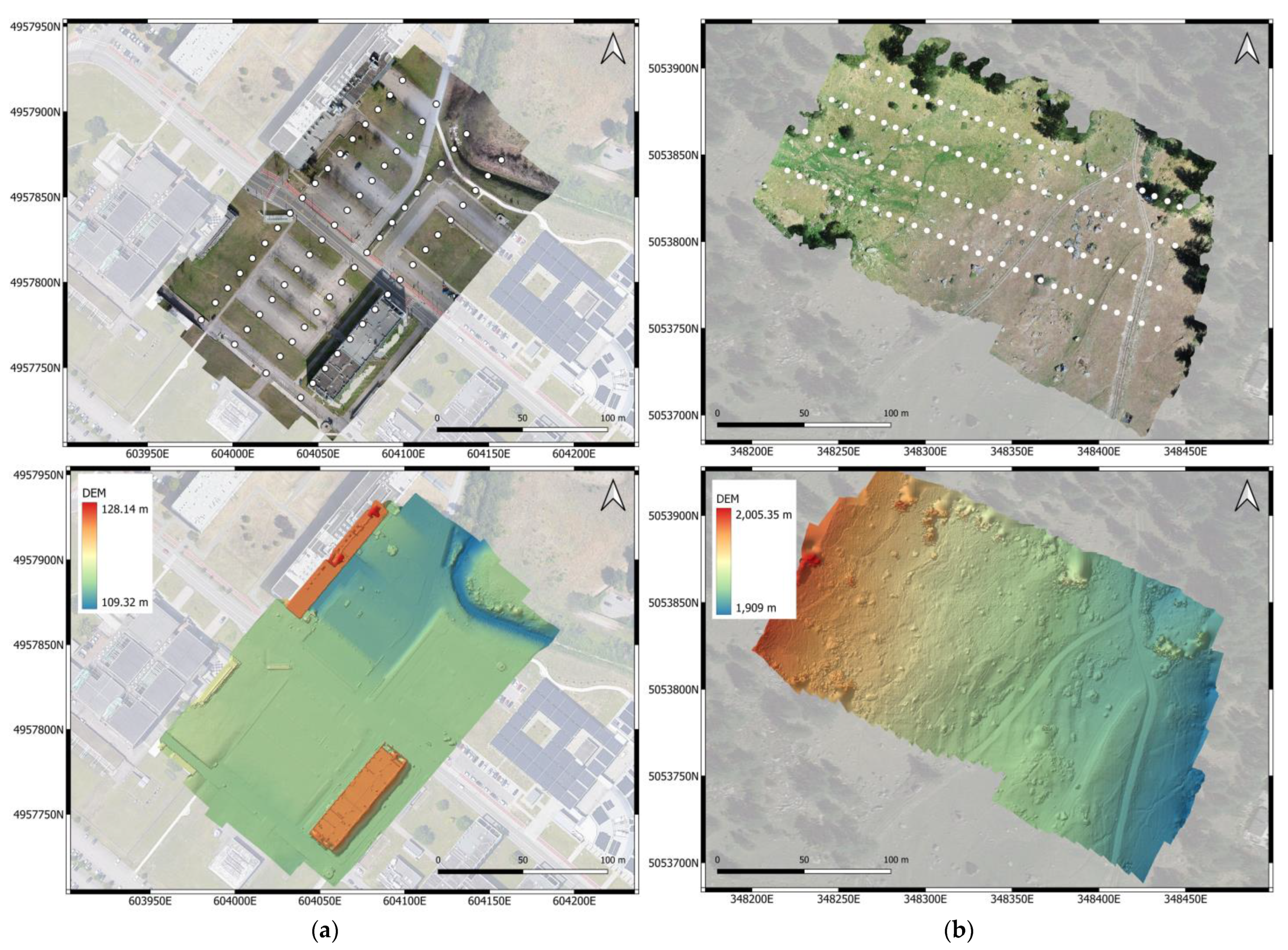
Two test fields (Figure 1) with different characteristics have been selected to possibly highlight an influence of the terrain morphology. The first site (Site A) is located on the Parma University Campus (44°45′259″N 10°18′55″E). The area, approximately 110 × 200 m wide, includes car parking lots, tarmac roads, meadows, and buildings and is mainly flat. Only on the north-west side is the terrain slightly downhill, with approximately a 2-m height difference with respect to the main area.
The second site (Site B) is located in Aosta Valley (45°37′16″N 7°03′17″E), in the municipality of Valgrisanche, and is approximately 160 × 300 m large. It consists of a pasture grassland with numerous boulders and a few trees, at an altitude of approximately 1900 m a.s.l. The terrain is sloping, with a total height difference of approximately 90 m.
2.2. Image and Reference Data Acquisition
On each site, the same flight plan has been executed by all platforms and repeated at three different speeds: 1 m/s, 2 m/s and 4 m/s in order to highlight the dependence of the RS deformations on flight velocity. While the 1 m/s speed was selected to experience small or perhaps negligible deformations, the maximum speed of 4 m/s looks indeed rather lower than the normal operating speed of drones. The reason for choosing this value is that the campus area is partly within the buffer zone of Parma Airport, where the maximum flight elevation a.g.l. is 40 m. Assuming a linear correlation between speed and deformation on the image, flying at 4 m/s at 40 m should experience an effect proportional to a more common flight setup of 10 m/s at 100 m a.g.l. On Site B, such constraints on flight elevation did not apply; however, it has been preferred to maintain a similar flight plan. To keep the number of trees in the survey area to a minimum, the strips have been flown along the maximum slope direction in “terrain following” mode.
Each block on both sites is composed of 4 strips flown, with the characteristics depicted in Table 2. Table 3 shows the ground sampling distance (GSD) for the different platforms.
Data processing followed the same pipeline for all the blocks, using the commercial software Metashape version 1.8.0. Image orientation was performed with “High accuracy” settings, i.e., processing the images at their original size without any downscaling to get accurate camera position estimates. The image coordinates of the tie points and of the targets (GCP, CP) have been assigned a precision of 1 pixel and 0.5 pixels, respectively. The interior orientation and camera model parameters were estimated with an on-the-job self-calibration procedure. Table 4 shows the reprojection errors obtained for all the blocks without any rolling shutter compensation.
Reference data for accuracy checks on object points has been provided by a total station survey at both sites. On Site A, 67 points have been selected and measured all over the area, with the large majority over manhole corners and approximately a dozen on signalised targets. In Site B, the coordinates of 47 targets of varying sizes have been measured. Given the characteristics of the surveying instruments, the target type and the distances involved, the accuracy of the point coordinates can be estimated to be better than 7 mm in all coordinates. In each test field, the target coordinates have been transformed with a 3D Helmert transformation from the Total Station local reference system to the national geodetic system UTM32-RDN (EPSG 6707) after the determination of a few well-distributed targets by NRTK GNSS measurements. In all the BBAs, the coordinates of GCP have been assigned a precision of 5 mm.
2.3. Test Overview
2.3.1. Analysis of Check Point Accuracy as a Function of the Number of GCP
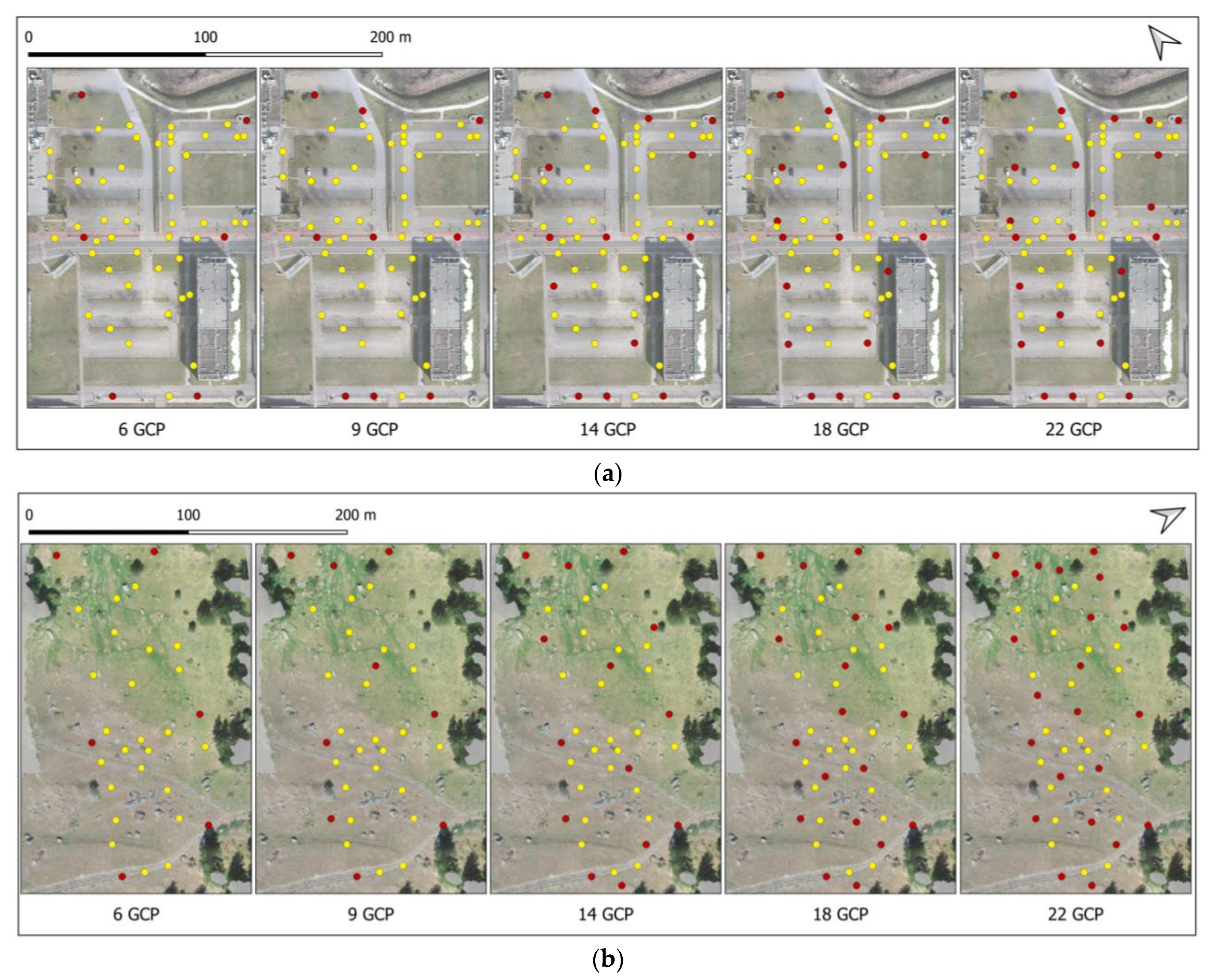
As it is well known that increasing the number of GCP is expected to improve block accuracy, the “fair” or “optimal” number of GCP for the specific project should be determined. While it is out of the scope of this paper to fully address this topic, two questions nevertheless arise: Is the optimal number of GCP for a given block dependent on whether the camera has a RS or not? Does such an optimal number depend on the way RS is modelled? To this aim, 45 checkpoints (CP) on Site A and 24 CP on Site B have been set to evaluate the accuracy changes as a function of the number of GCP. On both sites, the number of GCP fixed in the BBA has been increased from 6 to 22, in five stages: 6, 9, 14, 18 and 22 (Figure 2). For each number of GCP, a BBA has been executed in four variants:
- -
- without RS modelling and with an 8-parameter camera calibration model;
- -
- without RS modelling and with a 10-parameter camera calibration model;
- -
- with Metashape 2-parameter RS model and with an 8-parameter camera calibration model;
- -
- with Metashape 6-parameter RS model and with an 8-parameter camera calibration model.
To measure the influence of the number of GCP employed on the accuracy of object points, the decrease of the RMSE on CP due to a decreasing number of GCP fixed has been expressed, in each block and for each platform, as a percentage δ of the RMSE obtained in the most constrained BBA (i.e., the one with all GCP available fixed):
where
- RMSE(all): RMSE on CP of the BBA with all GCP fixed
- RMSE(i): RMSE on CP of the BBA with i GCP fixed, i = {22, 18, 14, 9, 6}
Ideally, the outcome of this analysis would clarify whether such an optimal number of GCP exists and, in particular, how it compares to that of a camera without RS. To this aim, the same procedure has been applied to the Phantom 4 Pro data in Cases A and B at both sites, though only for the 4 m/s speed flights.
2.3.2. Analysis of Rolling Shutter Compensation Model Performance
As a logical follow-up to the findings of the previous analysis, an optimal RS compensation procedure could be devised. To this aim, an in-depth analysis of RS compensation strategies has been performed for the blocks of both sites, considering different combinations of camera calibration models and the RS compensation models implemented in Metashape (v. 1.8.0). More specifically, the set of test cases reported in Table 5 has been executed.
Case A is the reference case for assessing the errors caused by ignoring the RS effect. Case B has been tested to check whether the deformation caused by the RS can be compensated by applying an affine transformation through the b1 and b2 parameters, as suggested by [23,28], and how much this expected affine deformation is dependent on the morphological characteristics of the terrain (flat or mountainous). Cases C and D have been addressed as refinements of Case B. In case C, only the parameter b1 has been adjusted to evaluate the contribution of this specific parameter and relate it to the alignment between the UAV motion and the sensor rows. Case D has been addressed to evaluate whether the estimation of b1 and b2 on an image-by-image basis could work better than their estimation of the whole block. The image-by-image parameter estimation allows, on the one hand, for the effective correction of image-dependent deformations, such as those related to slightly different speeds or the variation of scene depth over rough terrain. On the other hand, the introduction of a higher number of unknowns might weaken the BBA solution and require a denser control network.
In [25], Fraser introduces the affine correction term Δx to the x-image coordinate:
where and are coordinates that referred to the principal point.
The correction term appears, reformulated according to Metashape manual [24], in the last two terms of the coordinate u of the projected point in the image coordinate system:
where w is the image width (in pixels), is the principal point offset in the x direction (in pixels) and f is the focal length (in pixels). In this equation, x′ and y′ are dimensionless, therefore, for dimensional homogeneity, b1 and b2 are expressed in pixels.
Case E applies the 2-parameter correction model implemented by Metashape. This model estimates translational correction in the image plane for each frame and should eliminate the shift produced on the image coordinates by the sensor motion during readout. The expected correction effect should be comparable to that obtained using the 10-parameter calibration of Case D, with the correction parameters computed for every image.
Case F utilises the 6-parameter full correction available in Metashape. This model aims at correcting the deformation in the image coordinates by compensating for all possible camera movements (three rotations and three translations) during sensor readout. As in Case E, parameters are estimated image-by-image, introducing additional unknowns that might affect the stability of the block.
Finally, in Case G, the 10-parameter Fraser camera calibration model is applied concurrently to Metashape’s full RS correction model. The aim is to evaluate whether these correction models can be coupled, by considering the image-by-image estimation of Tx, Ty, Tz, Rx, Ry and Rz as further refinements of the correction obtained by calculating a single set of parameters b1 and b2 for the whole block, or whether this method only leads to an over-parametrising of the correction model.
In all BBAs and both sites’ 14 GCP have been fixed, as this number (though at first glance it might look too high relative to the test field size) has been found to deliver the expected degree of accuracy of the blocks.
To assess the effectiveness of the different methods in recovering the accuracy degradation caused by the RS, the errors on the check points have been computed and expressed in GSD units. The RMSE at checkpoints is given as the main reference value to measure accuracy.
2.3.3. A Simulation Study on RS Modelling with GNSS-Assisted Block Orientation
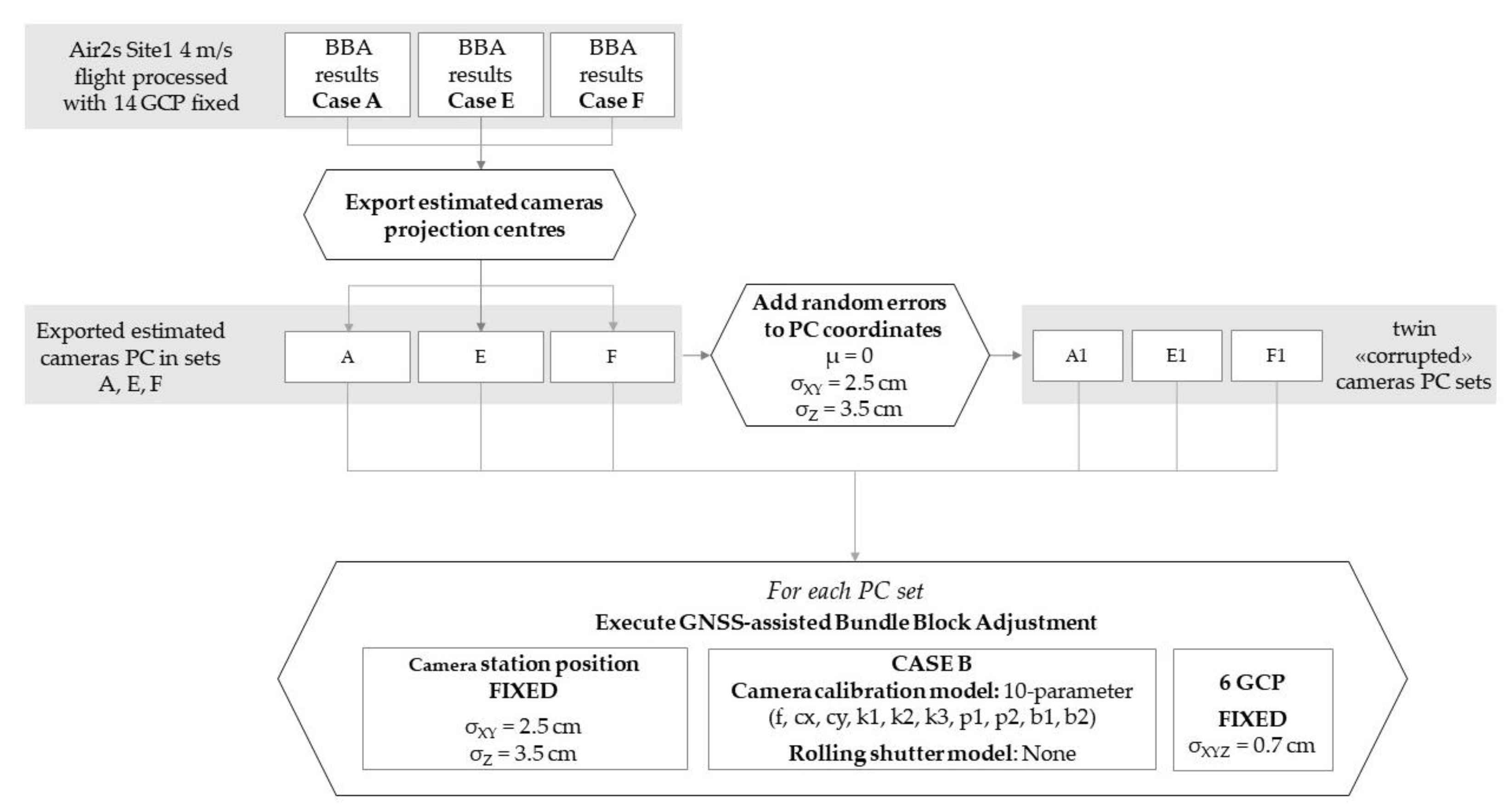
Through plug-ins modules from large drone manufacturers or do-it-yourself kits, users can render their UAV platforms RTK-capable. To empirically find out whether using cm-accurate camera positions from an on-board GNSS receiver while modelling the RS helps, a test with blocks flown with a RS drone and oriented with a GNSS-assisted BBA would be necessary. Unfortunately, we do not have a drone with such characteristics; however, the results of our tests provide some hints and a simulation study will be presented on this point. As the literature from GNSS-assisted BBA emphasises the correlations between internal and external orientation parameters and how they could affect ground coordinates [29,30,31,32], an analysis of changes in the estimated camera station elevations and in principal distance for varying correction models applied to the same block has been first executed. Based on the outcome of this analysis, a series of fictitious GNSS-determined camera projection centres (PC) have been generated and GNSS-assisted BBA have been executed for the Air2s 4 m/s flight in Parma, as illustrated in Figure 3.
As fictitious GNSS-determined PCs, those estimated by the BBA in Cases A, E and F with 14 GCP fixed have been selected. The rationale for this choice is that GNSS positions are not affected by RS, so the PC that would be determined by GNSS in a real case should be close to those of an adjustment where the RS effect has been reduced or removed. PC from Case A have, nevertheless, also been included, to control whether the tie points in the BBA manage to provide a coherent set of camera station positions despite being affected by RS deformations. Three further sets of PC (A1, E1 and F1 in Figure 3) have been generated, adding to the coordinates normally distributed errors with zero mean and standard deviation of 2.5 cm for horizontal coordinates and 3.5 cm for elevations, respectively.
The six sets of camera stations have been adjusted in GNSS-assisted mode, applying Case B camera calibration and RS correction models. In the BBA, the PC has been assigned a precision of 2.5 cm in horizontal coordinates and 3.5 cm in elevation, while the initial values of the camera rotations were set to zero in all adjustments. In addition, the coordinates of 6 GCP (none of them among the 14 GCP used to generate the simulated positions) have been fixed. The accuracy of the GNSS-assisted BBA has been measured by the RMSE on the CP.
3. Results
3.1. CP Accuracy as a Function of the Number of GCP
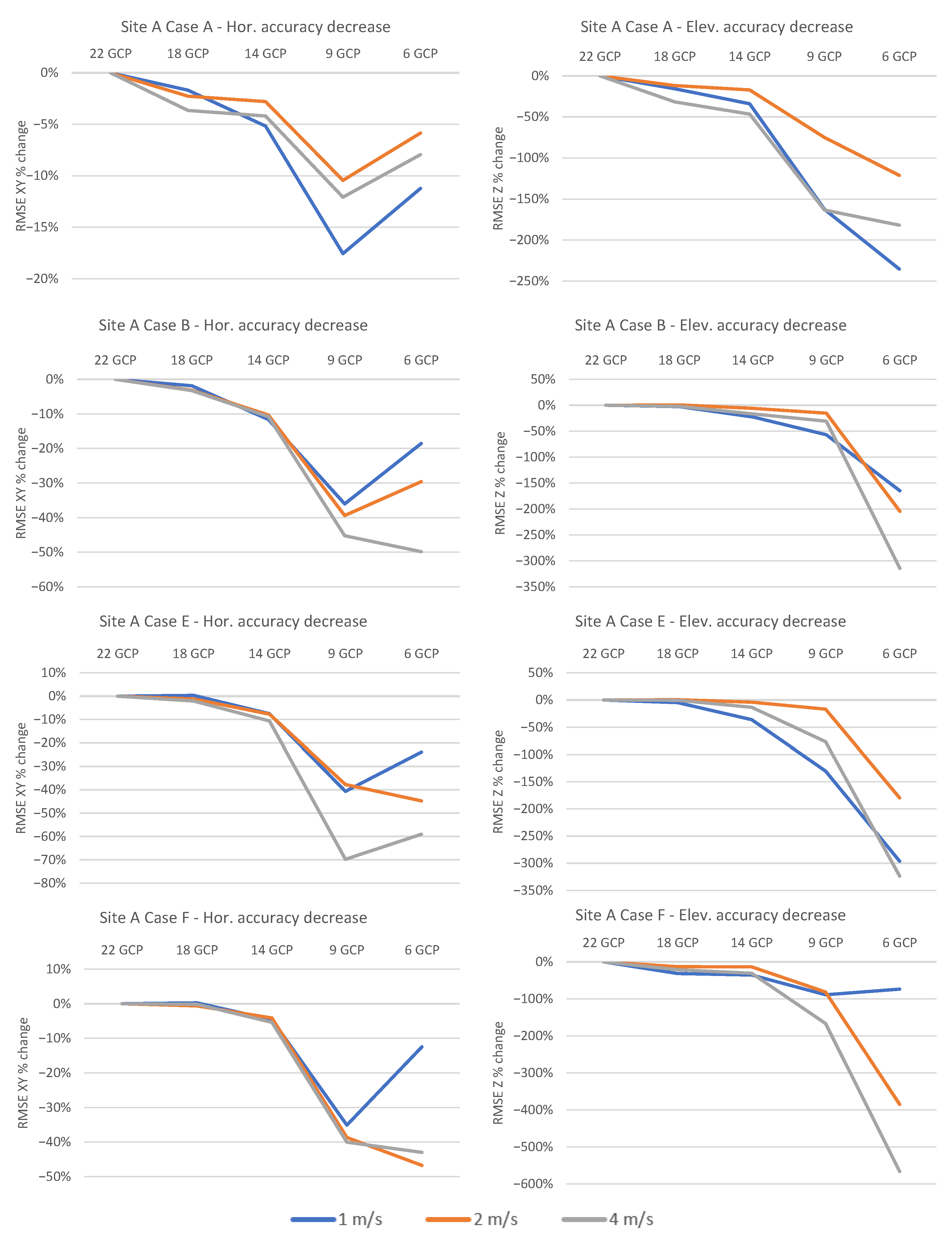
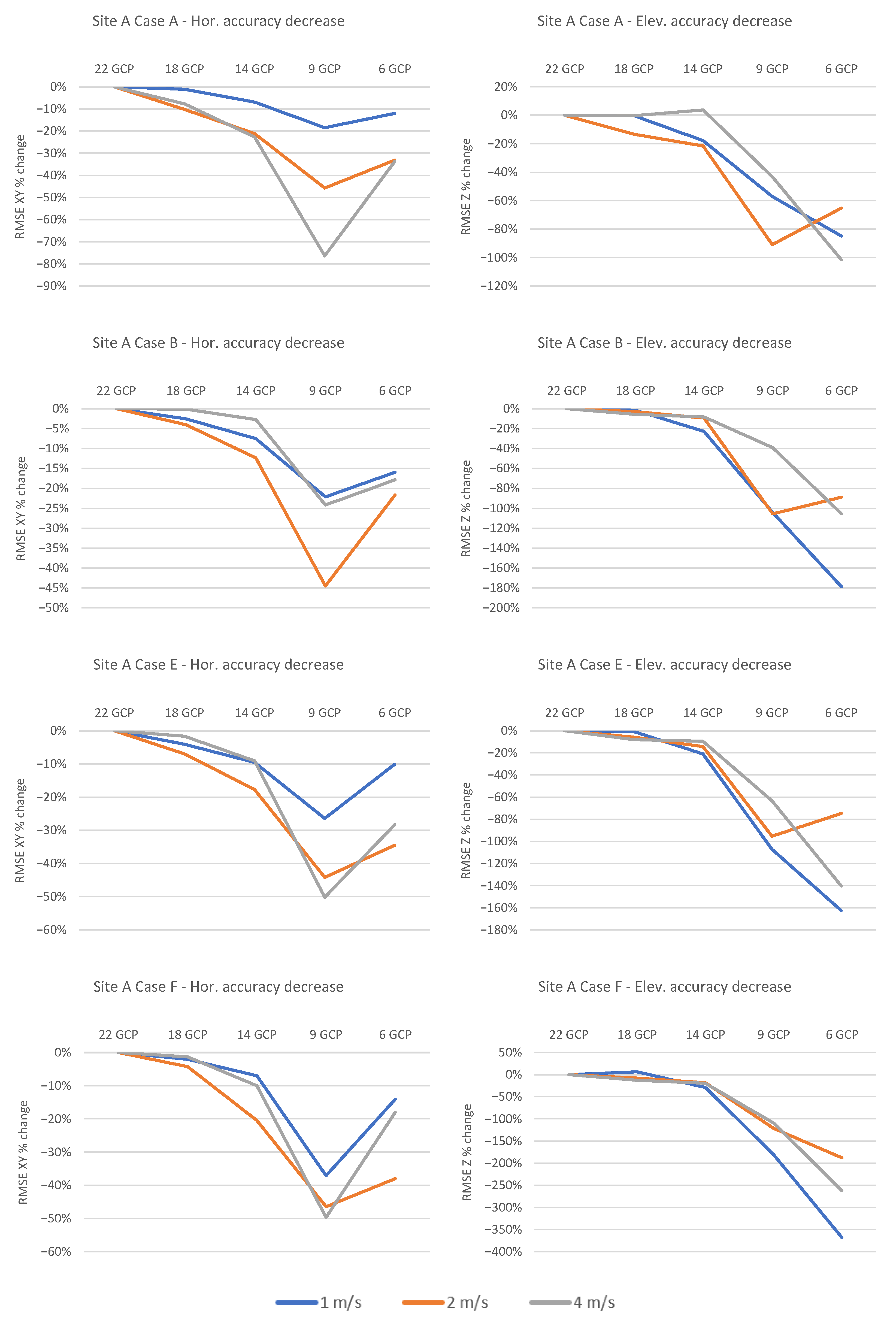
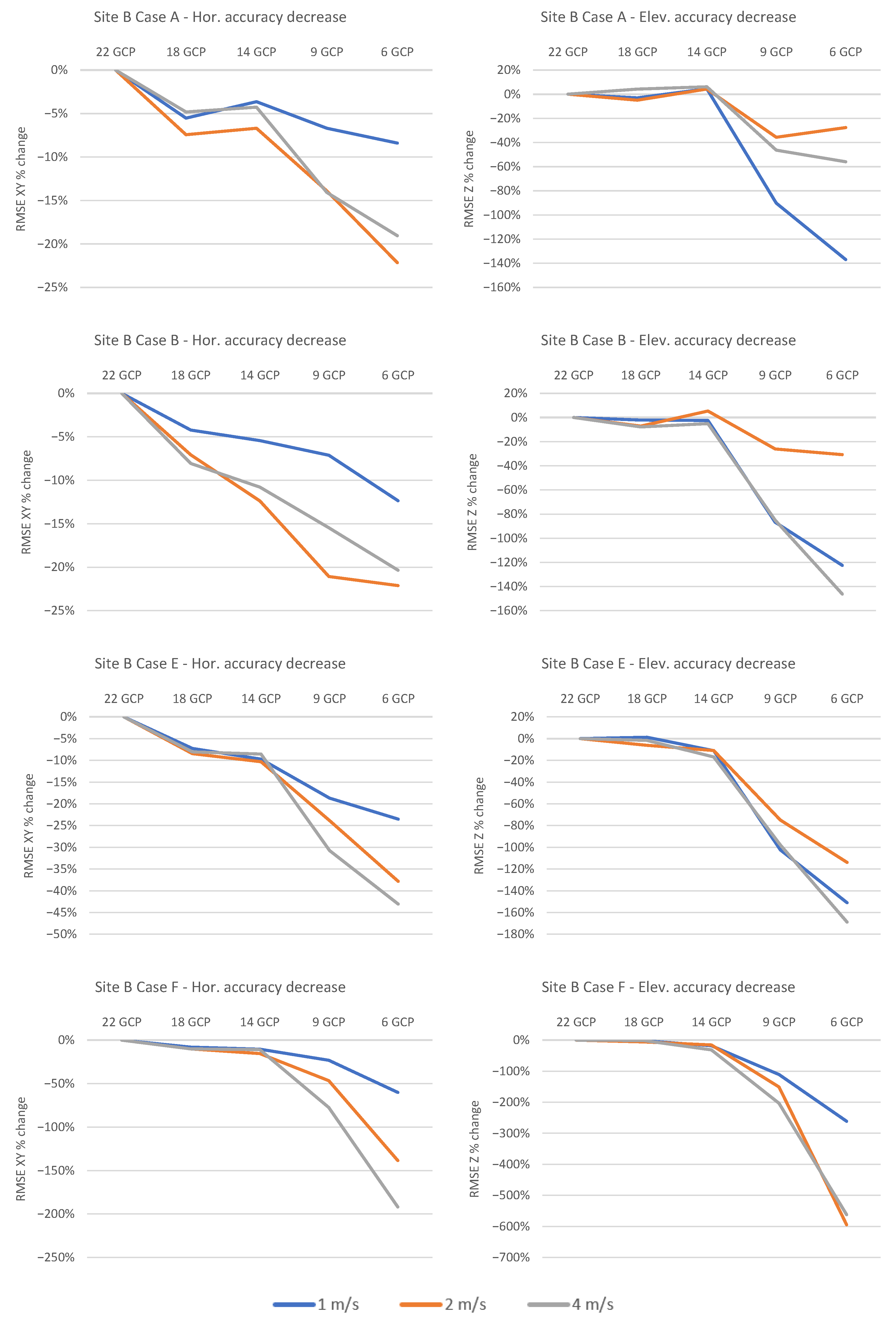
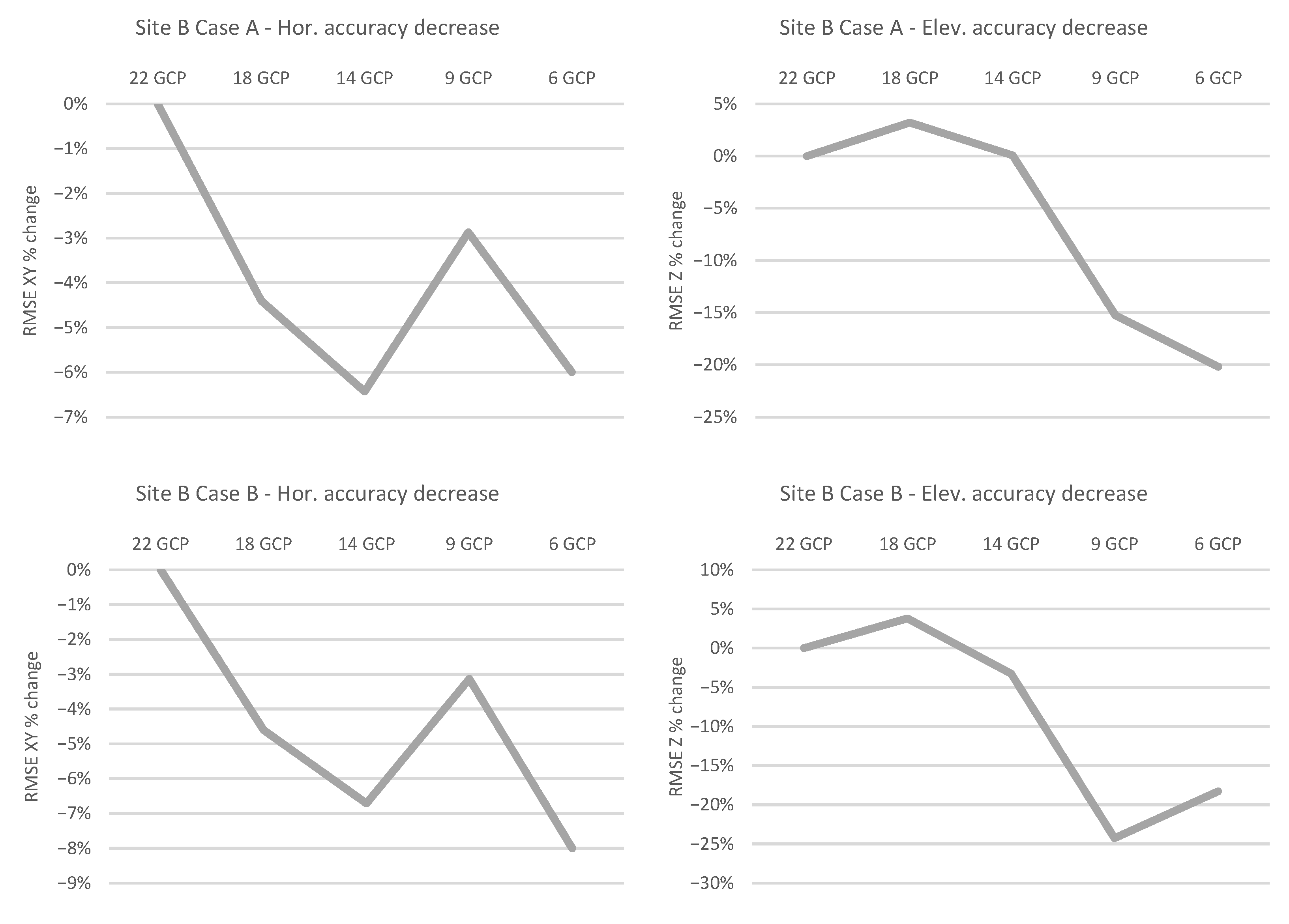
Figure 4 shows the graphs of the percentage accuracy loss δ from Equation (1) for horizontal coordinates and elevations in Cases A, B, E and F of Table 4. The graphs refer to the Air2s flights over site A; the same type of graphs, referred to Air2s flights over Site B (Figure A1) and to the Mavic Mini platform over both sites (Figure A2 and Figure A3) are reported in Appendix A. Their trends look broadly similar to those depicted in Figure 4, though with some differences that will be pointed out. From the examination of the graphs, a few considerations can be drawn, though it must be admitted that the interpretation is not always clear-cut.
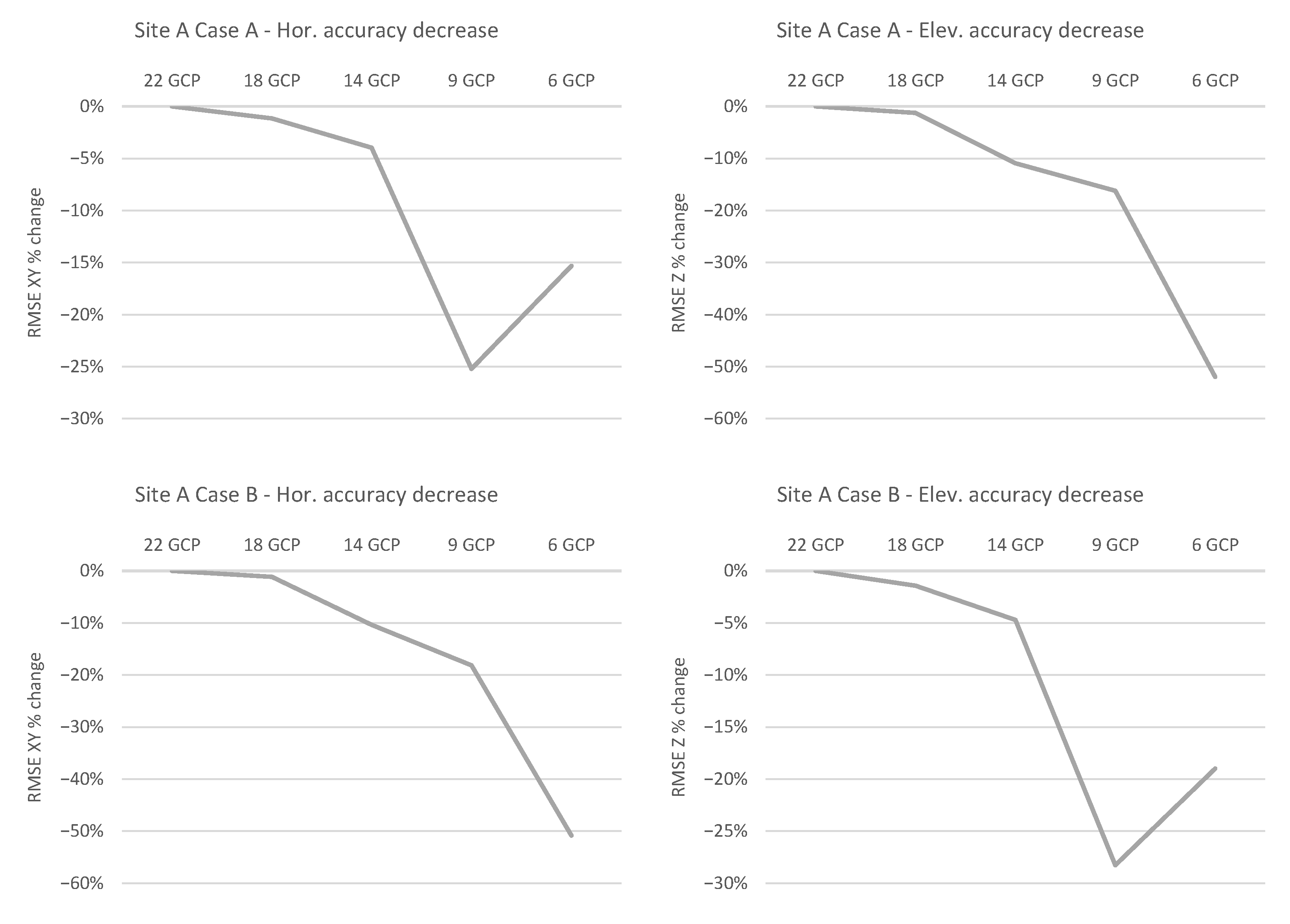
The number of GCP used matters a lot: using too few of them might lead to quite a significant loss of accuracy, up to almost six times with respect to the case with (very) dense control, independent of the RS modelling applied. Though with varying evidence, at both Site A and B and with both platforms, the accuracy loss is negligible or limited to 14 GCPs or more. This is a value that looks perhaps higher than one would expect at first glance, given the small size of the test fields and a strip length of approximately 20 images. As this might depend on the experiment setup and not on the RS, ideally the “right” number of GCP for the blocks in the absence of RS should first be found. Obviously, this is not possible, but a clue can be derived by computing δ in Cases A and B with the Phantom 4 data at both sites (see Figure A4 and Figure A5 in Appendix A). It turns out that, compared to the very dense control with 22 GCP, the maximum accuracy loss for the Phantom 4 is 50% at Site A with nine GCP and 25% at Site B with six GCP; to the contrary, with 14 and 18 GCP, the accuracy loss is always smaller than 11%. In other words, in our tests, nine GCP could be acceptable with a global shutter sensor but might not be sufficient for one with RS.
Returning to the general analysis of the δ graphs, most depict a sort of knee curve as a function of the GCP number: a roughly flat section from 22 to 14 GCP and then, mostly after a marked slope change at 14 GCP, a monotonic downward trend. The only notable exception is for the horizontal coordinates in Site A, where in all processing cases and at all speeds both platforms show a minimum for δ at nine GCP rather than at 6 GCP (notice that the six GCP set is derived removing three points from the nine GCP set).
The horizontal coordinates accuracy loss is generally limited, below 45% in most Cases, irrespective of platform, site and speed. The only exception is Case F in Site B, where with six GCP the loss is close to 200% for the Mavic and 140% for the Air2s. This fact is probably due to some interplay between the method and the site characteristics, as in both platforms the three curves show a similar pattern and the same order, i.e., increasing accuracy loss while platform speed increases from 1 m/s to 4 m/s.
The accuracy loss in elevation, to the contrary, is normally quite large for blocks constrained with only none or six GCP, without applying any correction (Case A). The astonishing fact is that, in such cases with poor ground control, trying to correct the RS yields the largest accuracy losses, with the ad hoc parametric models of Metashape performing even worse than the 10-parameter camera calibration model. The worst δ value with 6 GCP was registered for the Mavic at site B, Case F with a 594% loss. The worst for Air2s is a 566% loss at Site A, also in Case F.
From our tests the platform speed does not show a clear influence on δ. With dense control (22, 18 and 14 GCP) for both Air2s and Mavic the curves are in most cases close to each other; with 9 and 6 GCP the picture is not uniform: sometimes the curves remain close, though in the majority they diverge. In any case, the amount of loss for a given Case and Site is not necessarily related to the speed. Indeed, though one would expect the largest loss for any GCP number to be registered by the 4 m/s flight and the smallest by the 1 m/s flight, this only happens in seven cases out of 16 for the Air2s and 4 out of 16 for the Mavic.
3.2. Rolling Shutter Compensation Strategies
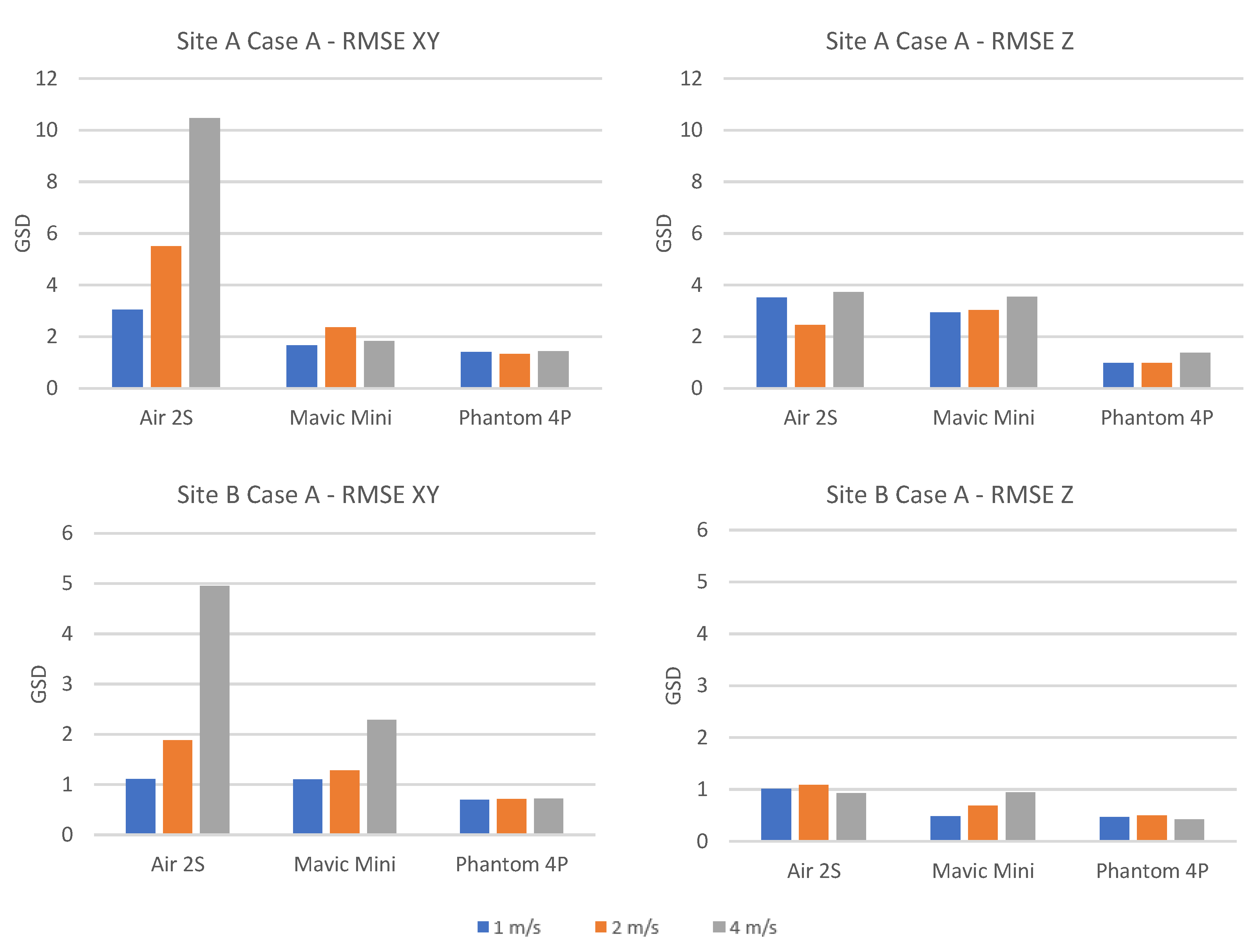
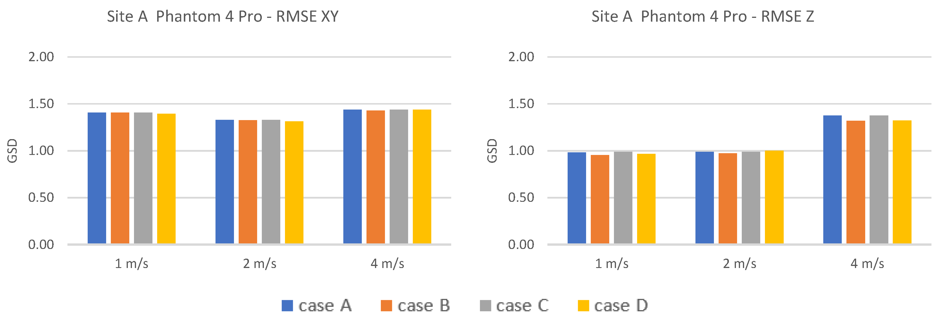
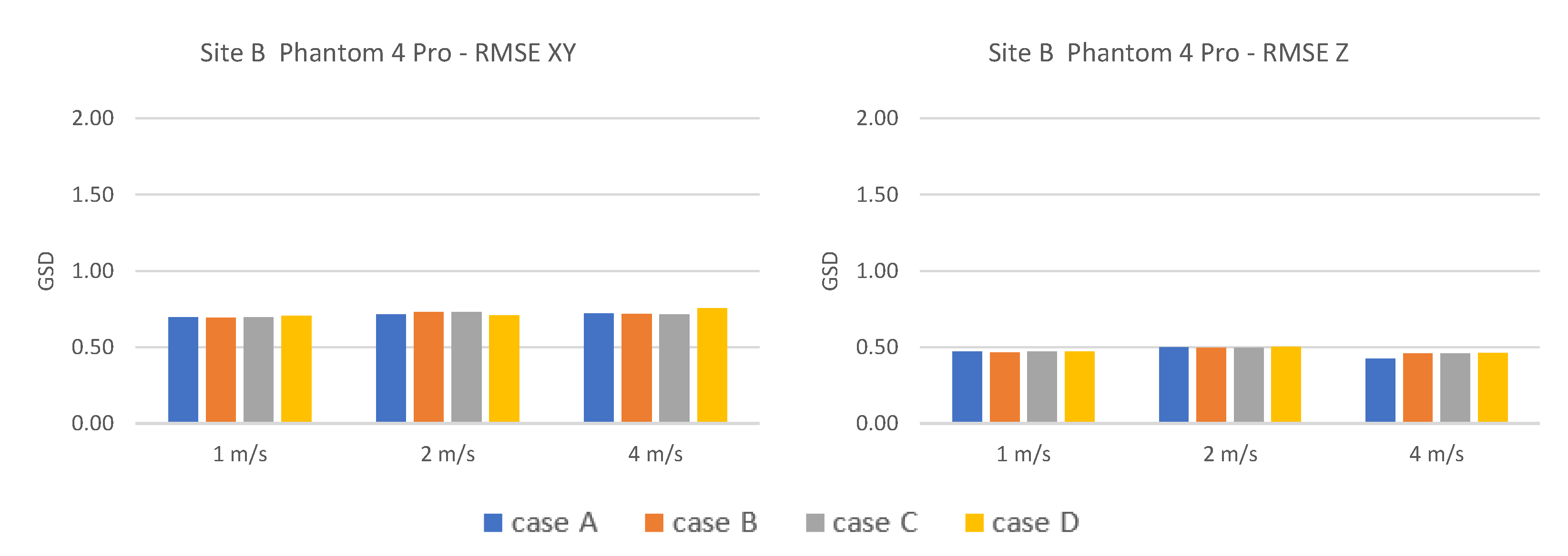
Figure 5 shows the graphs of the RMSE on CP in Case A, for all the platform tested and in both Sites, to evaluate the effect that RSs have on the object 3D reconstruction. The RMSE are expressed in GSD units for a better comparison among the platforms and are provided for horizontal coordinates and elevations independently.
As expected, the RMSE increases the faster the UAV speed, since higher speed increases deformations in image coordinates, resulting in less accurate point coordinates. Horizontal coordinates are the most affected by speed, except for Mavic Mini in Site A. The magnitude of accuracy loss varies with the platform and is particularly high for Air2s, with a 244% change in Site A between the slowest and the fastest flight. Mavic Mini shows RMSE increase on horizontal coordinates of 102% in Site B. To the contrary, the RMSE variation with speed is quite negligible for Phantom 4 Pro.
It is worth noting that RMSE values at Site A are about twice those at Site B for all platforms (i.e., including the Phantom 4 Pro) despite the GDS being smaller in Site A. This can be related to the different topography of the two Sites and to the slightly different block geometries. Site B is mountainous with an average slope over the surveyed area of 30%, so the high depth changes inside the scene could have strengthened the camera calibration parameters’ estimation. In addition, the higher side overlap, compared to Site A, increases the number of projections per GCP (6 and 13 on average for Site A and Site B respectively) and may have helped to strengthen the blocks, improving the accuracy on ground.
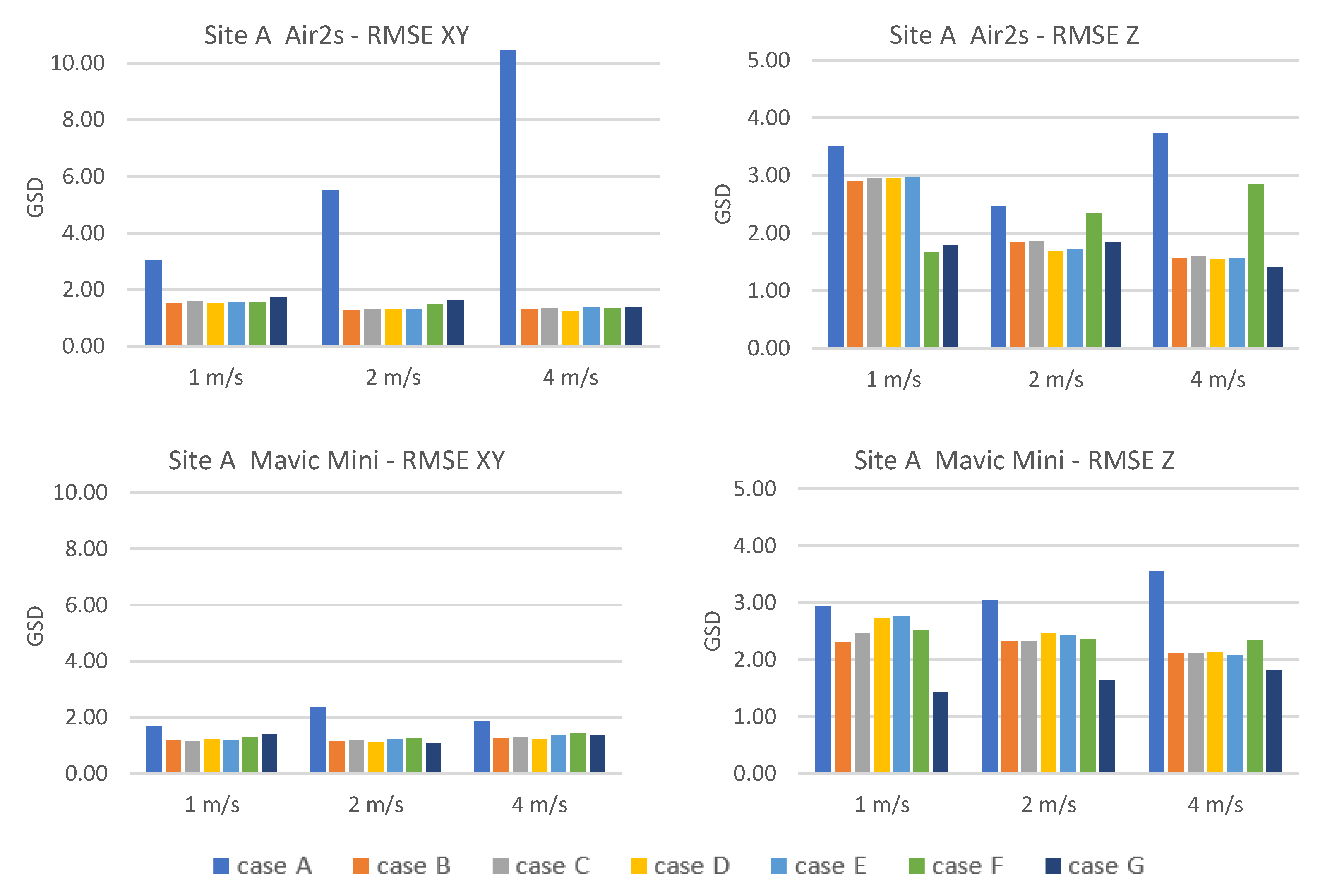
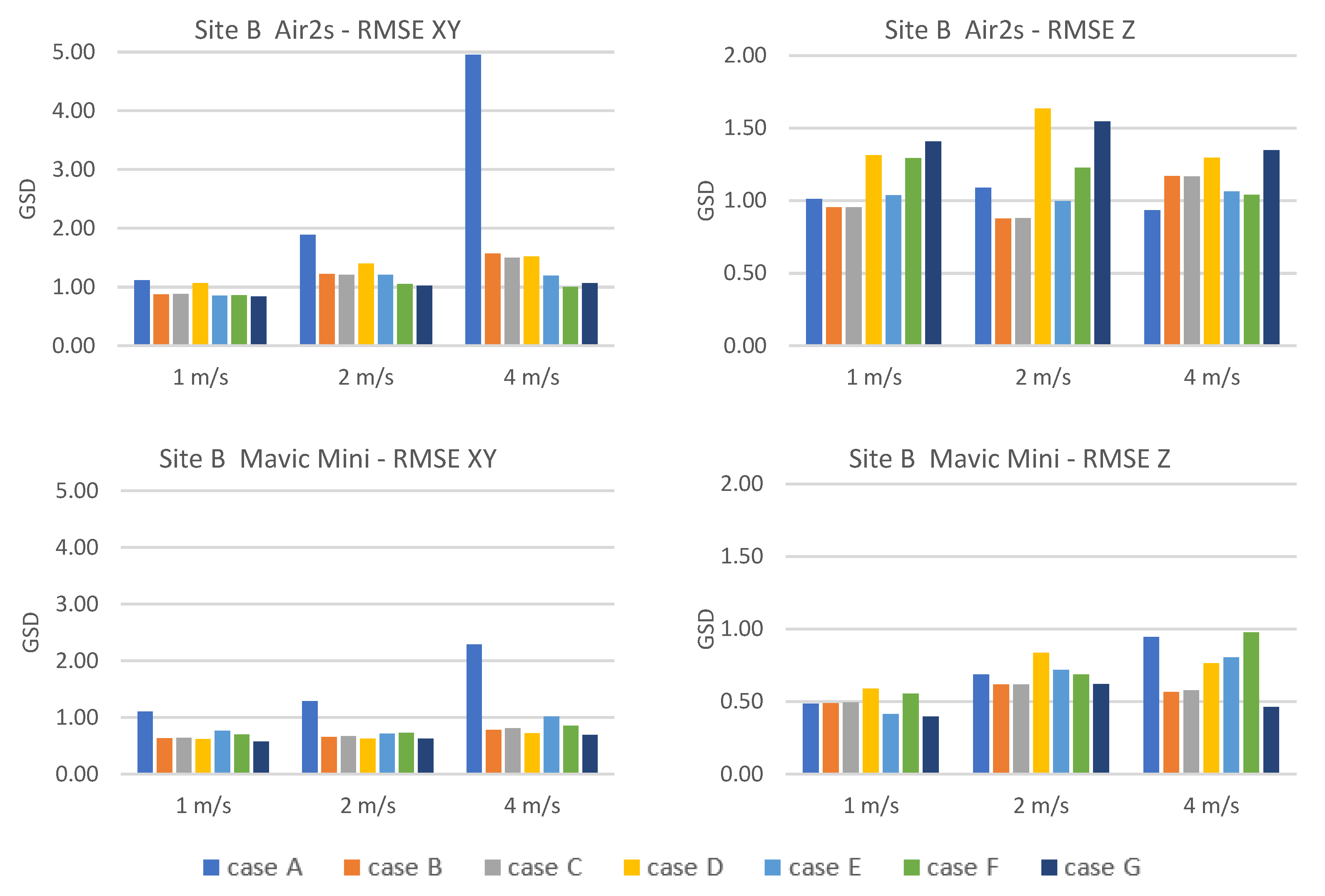
Figure 6 and Figure 7 compare the performance of Cases A to G (see Table 5) in RS effect compensation. The graphs show the RMSE on CP for horizontal coordinates and elevations grouped by Site and refer to the Air2s and Mavic platforms; those related to Phantom 4 Pro, provided in Appendix B (Figure A6 and Figure A7) for comparison, are restricted to Cases A, B, C and D, since the drone is equipped with a global shutter camera.
Overall, the graphs depict two different behaviours for horizontal and vertical coordinates.
Horizontal coordinates generally benefit most by the RS correction models, especially when the RMSE in Case A is very high. For instance, the RS effect is particularly strong in Air2S blocks, even at low speeds, and all the applied correction models greatly reduced the RMSE (e.g., from 10 GSD to 1 GSD for the block flown at 4 m/s). The positive effect of the correction models, on the other hand, is less evident in cases where the RMSE in Case A is already quite low, as for the Mavic, where is around 1 GSD.
Vertical coordinate accuracy, on the contrary, is less improved by correction models, maybe because of the already very good RMSE in Case A along the Z-direction.
Looking deeper in the contribution of each Case, the application of the extended Fraser camera calibration model (Cases B, C and D) proved to be effective in RS compensation by applying a scale transformation to the image coordinates in flight direction. As expected, the influence of the shear parameter (b2) is negligible: Cases B and C perform roughly on a par, demonstrating that only the parameter b1 is effective. The corrections provided by Cases B and C on XY coordinates always improve the RMSE, with percentage gains between 20% and 87% compared to Case A. In contrast, along the Z direction, although Cases B and C are generally improving with gains up to 50%, for the Mavic Mini block at 1 m/s in Site B these Cases perform the same as Case A, while for the Air2S block at 4 m/s in Site B, worse. It is worth noting that, at Site B, the effects of the correction on elevations are less evident due to the already very low RMSE of Case A (1 GSD for Air2S and 0.5 GSD for Mavic Mini), which make the influence of the models less significant and readable. In addition, the above-mentioned worsening amounts just to +0.01 and +0.23 GSD compared to Case A, which is far below the expected accuracy and completely negligible in all applications.
Estimating the value of b1 and b2 on an image-by-image basis, as tested in Case D, has, instead, proved to be not particularly cost-effective. Over flat terrain, the RMSE is quite comparable to that of Cases B and C, while, contrary to the expectation, over rough terrain the RMSE is higher and, in elevation, even higher than Case A. Therefore, although on rough terrain the image scale changes considerably even within the same frame, estimating a single set of affine parameters for the whole block seems to be preferable.
Case E has very similar behaviour to Cases B and C in XY, except for the blocks flown at 4 m/s in Site B, where Air2S corrections are greater compared to the Mavic Mini. However, these are still very small variations, which correspond, in absolute values, to −0.38 GSD and +0.24 GSD respectively, compared to Case B. In altimetry, on the other hand, the behaviour is more variable, albeit with slight deviations in absolute terms from the values obtained with Cases B and C.
Case F performs similarly to the previous Cases in XY, apart from the block Air2S—4 m/s in Site B, where it provides RMSE 0.5 GSD lower than Case B. In altimetry, Case F provides, on average, smaller corrections than previous Cases and in Site B it performs even worse than Case A, albeit with RMSE increase lower than 0.3 GSD.
Case G has a more variable and apparently Site- and coordinate-related behaviour. In XY, at Site A, it gives generally the worst outcomes (except for Mavic Mini at 2 m/s), while at Site B, it gives the best results. In altimetry, on the contrary, at Site A it gives the best results, while at Site B the worst, with RMSE increases of up to 45% compared to Case A.
To summarise, all tested methods proved to be very effective in RS compensation as far as the horizontal coordinates are concerned, with overall RMSE decrease compared to Case A up to 87% (depending to the block) and differences in performance among the Cases lower than 15%. As for the elevation, instead, the behaviour is more variable with no clear evidence of a best performer. Indeed, sometimes the application of complex correction models with parameters estimated image-by-image (D, F and G) proved to be detrimental.
Contrary to the expectations, no clear improvements on reprojection errors appears after applying RS compensations.
Finally, the application of the full camera calibration model (Cases B, C and D) to Phantom 4 Pro data (see Figure A6 and Figure A7 in Appendix B) did not produce significant improvements of RMSE on CP.
Parameters’ Value Evaluation
A further analysis was carried out on the parameters estimated in the correction methods applied.
As far as b1 and b2 are concerned, both parameters are statistically significant with respect to their standard deviations, though the improvements brought by b2 on RS correction is negligible. On the other hand, b1 proved to be very effective, with consistent and reliable behaviour.
The estimated b1 values are always negative, which can be viewed as a stretching of the sensor in the Y direction (flight direction).
Table 6 shows the estimated b1 values for each block. For the UAVs equipped with RS sensors, the values of b1 are proportional to the flight speed. For the blocks processed in Cases B, C and D (where the RS compensation relies only on camera calibration parameters), b1 doubles as the speed doubles; for Case G, instead, the value of b1 always increases as the speed increases but without direct proportionality. In this Case, in fact, the corrections rely on the mutual influence of camera calibration parameters and the six parameters of the Metashape full-compensation model, therefore the increase of b1 values along with the speed is less pronounced.
In contrast, the correlation between b1 and speed cannot be observed in the tests on Phantom 4 Pro, where even the RMSE on CP (see Figure A6 and Figure A7 in Appendix B) does not show considerable accuracy variations according to the flight speed.
Besides the speed, the magnitude of b1 seems to be related to the drone and, therefore, to the deformation caused by the inner structure of the sensor. The Air2S, which was more affected by RS (see Figure 5), recorded the highest b1 values; the Mavic Mini generally halved these values, while for the Phantom 4 Pro b1 values are much smaller (by at least two orders of magnitude at Site A and one order of magnitude at Site B) and have discordant signs.
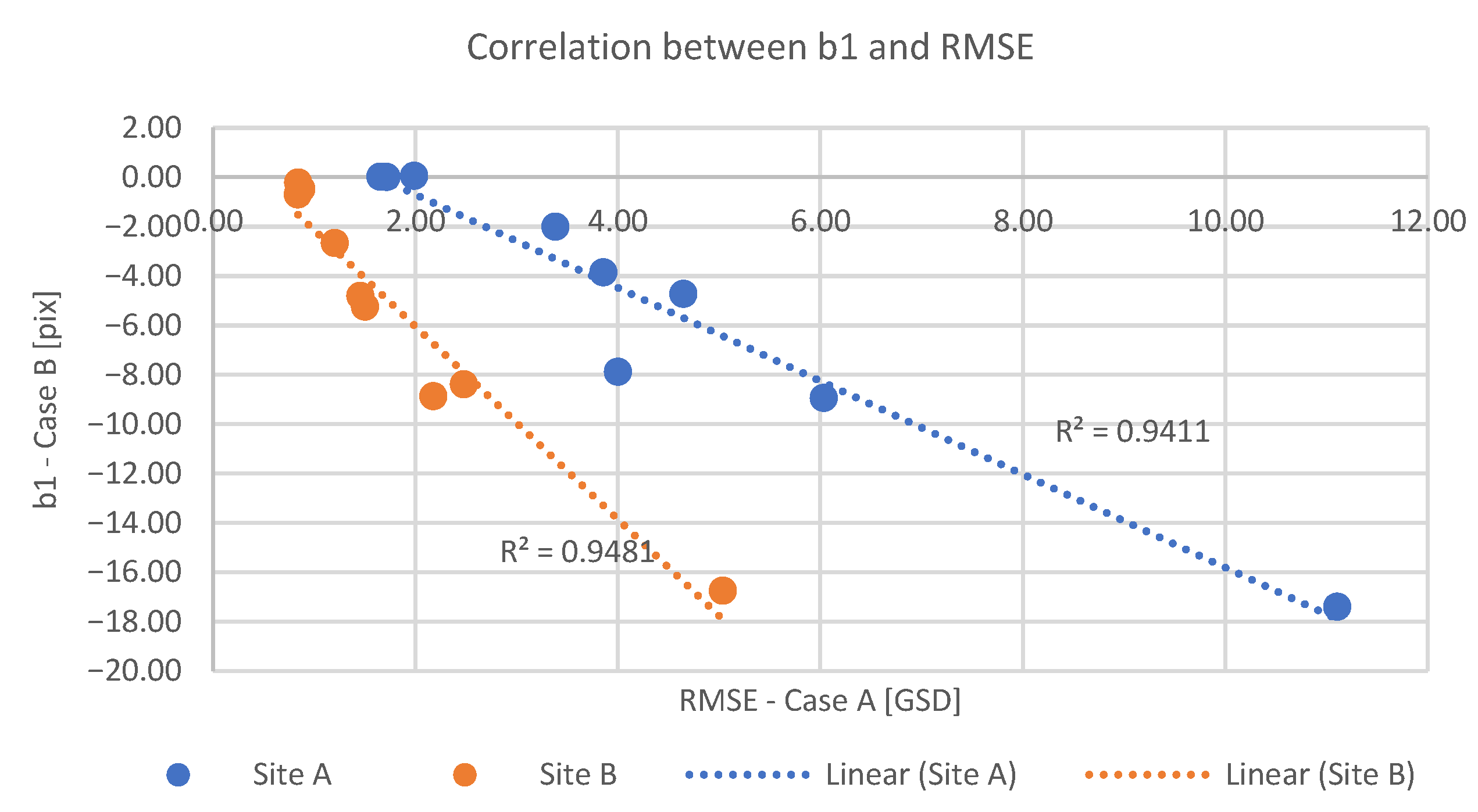
Figure 8 shows the correlations, for all the drones and flight speeds, between the RMSE on CP (xyz coordinates) in Case A and the values of b1 computed in Case B for the same flight. The correlation is evident (−0.97 for both sites, with R2 = 0.94) and confirms that a large portion of the RMSE is due to the RS effect and that just the b1 parameter is effective in correcting it. In fact, after corrections, the RMSE is leveraged even among all the drones.
As for the parameters Sx, Sy and Tx, Ty, Tz, Rx, Ry and Rz, used by the two Metashape correction models, respectively, only a cursory analysis of similarities between the values of the b1 and b2 parameters can be made since the underlying mathematical model is not known.
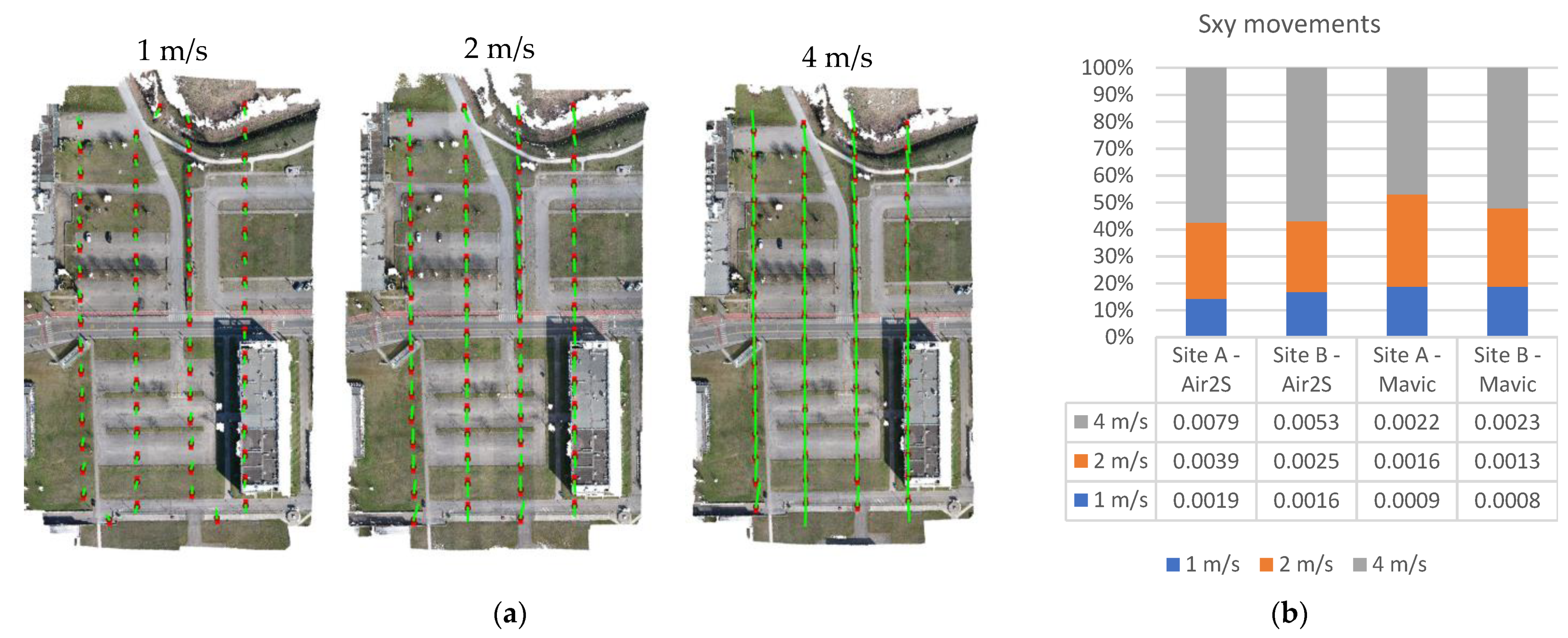
Sx and Sy are documented as “axis shifts in X, Y in the plane of the photo” and are estimated image by image. From the experimental tests, the result was, on average, proportional to the flight speed and higher for the Air2S platform (the most affected by RS). Figure 9a provides a graphical representation of camera movements for Air2S in Site A at different flight speeds. Figure 9b shows the values of the combined Sx and Sy shifts (averaged over each block) at different speeds for each drone and site and their 100% stacked bar chart to highlight their relative proportion at different speeds.
These shifts in the image plane can be conceptually and empirically equated to the b1 and b2 parameters, which, in the Metashape mathematical formulation, represent a length expressed in pixels. A test was performed comparing the values of b1 and b2 computed image-by-image in Case D with Sx and Sy estimated for the same images in Case E. Table 7 shows the correlation between b1-Sy and b2-Sx, which, for most of the blocks, is over 90%, as a confirmation of the comparable effects provided by Case D and Case E.
As far as Cases F and G are concerned, no relationship is shown between the magnitude of correction and speed, nor is there a correlation between the translational component and the corresponding shifts obtained with Case D and Case E. Therefore, without clear documentation of the mathematical formulation, it is not straightforward to infer how the Metashape full-correction model operates on BBA.
3.3. Rolling Shutter and GNSS-Assisted BBA
Table 8 reports the differences, with respect to Case A, of the principal distance and the camera projection centres’ average elevation over the whole block for Cases B, E and F, respectively, all adjusted with 22 GCPs fixed for flights. As can be seen, the differences are quite relevant in absolute terms for both variables and are also strongly correlated, whether considering the whole Table 8 dataset or dividing it according to platform, flight speed or site. The correlation coefficient between principal distance and average elevation differences is never below 0.98. Though the values in the table refer to the most constrained BBA, the pattern is quite similar also with less GCP fixed, namely with 18 and 14 GCPs (the last being the “best choice” for block control, as discussed in 3.1).
Apart from correlation, there are a few patterns that can be spotted in Table 8. Speed clearly matters, though changes are not proportional to speed. As more speed means more RS effects, this is perhaps an indication that the estimation becomes less stable for larger RS deformations. However, it should be noted that these large differences in changes for the same case at different speeds do not affect much of the accuracy on the ground; indeed, for the same correction method, the differences in RMSE for all CP coordinates are in most cases below 0.5 GSD at any speed.
Another (a bit puzzling) fact is that either the site morphology or the block geometry seems to matter: at Site A, all changes are negative for both platforms and all cases, while changes are all positive at Site B. There are two exceptions: the first, Case F for the 1 m/s speed, is only an apparent one as it follows the “site rule” simply with a different sign; Case F for the 2 m/s speed, instead, is a true exception, as it is negative at Site B for the Air2s and positive for the Mavic. This notwithstanding, all six flights of the two platforms correct both the focal length and projection centre elevation in the same direction, though in very different amounts.
As anticipated in 2.3.3, the camera PC of the Air2s flight at 4 m/s speed at Site A, computed from the BBA in Cases A, E and F, has been used as a fictitious GNSS-determined PC. From these three original sets, three more were obtained by adding random errors to the coordinates. Each of the six sets of camera stations has then been processed in a Case B GNSS-assisted BBA, assigning the PC a precision of 2.5 cm in horizontal coordinates and 3.5 cm in elevation. In addition, the coordinates of six GCPs have also been fixed. Table 9 reports the RMSE on the CP for the six adjustments. In the upper part, the RMSE refers to the original, uncorrupted PC, and in the middle to the camera positions with errors. As a reference for the comparison with a well-constrained, GCP-only, block adjustment, the RMSE on CP for Case B with 14 GCP is reported in the last row of the table.
As it can be seen, the RMSE on the CP for pseudo-GNSS-determined stations with the RS effect modelled is in the same range as a denser GCP-only block control. With fictitious camera stations coming from an adjustment without RS correction (PC sets A and A1), the errors are slightly larger, especially in elevation. Adding random errors did not change the results significantly. An additional test has been performed by fixing only one GCP in the block middle, as suggested in [29]. In this case, the RMSE increased markedly, to more than 4 cm and up to 7 cm in elevation.
4. Discussion
Our investigation started with the influence of GCP density when applying or not applying RS corrections. At least for all the correction models tested in this paper, an optimal GCP density should be found, as too few points may cause large errors, while adding more after a certain number does not bring improvements. On this point, the results we found are broadly in agreement with [26], wherein the tests over a square block (1 km2, approximately 1000 images), using more than eight GCP did not improve the horizontal coordinate accuracy by more than 0.9–2.1 GSD; elevation accuracy improved much less or not at all. On the other hand, in a rectangular block (0.2 km2, approximately 400 images) with eight GCP only, the accuracy was already better than one GSD in horizontal coordinates, while in elevation, it ranged between 2.6 and 8.3 GSD. Though the GCP density is quite different from our experiment, the conclusions are similar, in particular, that too few GCP affect primarily the accuracy of elevation. In [23], in an area 200 × 150 m wide, out of 15 points, 8 and 7 were used alternately as GCP and CP in each of the various tests; the RMSE changed up to more than 50% when switching CP and GCP. Though taking into account the small GCP and CP sample sizes, this also hints that GCP layout matters and cannot easily be optimised. Still, in the [23] paper, it has been mentioned that in the block corridor case, only the MicMac and the 10-parameter camera models were effective, while Metashape had large errors, especially in elevation. Though we did not investigate a corridor case, as the number of GCP used (five over a 400-m-long strip) is limited, this could be seen as consistent with our analysis of errors in elevation with poor ground control.
As far as the investigation on the effectiveness of the different strategies for RS modelling is concerned, our experiments confirm the close dependence between the amount of RS deformation (caused by speed or sensor characteristics) and the effectiveness of correction models, as already pointed out in [8]. We may expect that the quality of the sensor and the technical specification might result in different residuals on the CP. Surprisingly, the Mavic Mini performs better than the Air2S, at both sites and at each speed, although the Air2s sensor is nominally of higher quality. This gap in performance could be related to the different readout times of the two sensors. Otherwise, if the line readout time were the same, it might depend on the different resolutions (5472 × 3648 and 4000 × 2250 for the Air2S and Mavic Mini, respectively), which results in a longer readout time.
As far as the computational load of the different correction models is concerned, from the report logs, there is no noticeable difference among the methods. On the other hand, the time taken to estimate the parameters and complete the BBA, compared to other tasks such as key point extraction and matching, is negligible: a matter of seconds compared to several minutes for the whole SfM procedure.
The analysis of the parameters of the different RS models confirms that the largest deformations are generated by the camera translation and affect horizontal coordinates more than elevations, as observed in [9]. Therefore, methods modelling only translations (Cases B, C, D and E) proved to be fully effective, while adding camera rotations to the models (Cases F and G) did not bring improvements. It has also been found that, while modelling RS deformation is always beneficial on horizontal coordinates, using elevation correction models with many parameters (e.g., F and G) or computing parameters on an image-by-image basis can lead to accuracy losses.
From our tests, what was observed in [23] is confirmed, and, in most cases, a specific correction model is not necessary since the deformation caused by RS can be adequately modelled by applying the extended Fraser camera calibration model (Case B and Case C) even in the mountainous Site B, where it was expected to be detrimental.
The findings in 3.3 actually suggest that modelling the RS distortions, whatever the mathematical model adopted, may bring some instability to the estimation of interior and exterior orientation parameters by the BBA. The number of deviations of the parameters from the “unperturbed” solution is quite variable, from negligible to implausibly large, though, as already remarked in 2.3, the RMSE on CP remains limited in all cases. However, in [23], it has been found that the correction models of both Metashape and Pix4d failed to be effective in the case of corridor mapping, resulting in high residuals on CP coordinates, so the possibility that ground coordinates could be affected cannot be ruled out.
One may wonder whether the reason for the large variations in the camera calibration parameter comes from a weak block geometry. In fact, this is not the case for two reasons. At each site, though acquired only in a pseudonadiral case, the blocks contain images that feature conspicuous height differences: at Site A, the two strips at the block sides include buildings of different heights (from 8 to 12 m against a relative flight elevation of 40 m), while at Site B, the images are taken over a steep slope. These are maybe sub-optimal conditions, but still adequate to perform self-calibration, according to [33]. Moreover, the flights with the Phantom 4 at both sites have also been processed in Cases A and B with a variable number of GCP, and the changes in the focal length are in the order of one pixel for 1 m/s speed and a bit larger (up to three pixels) for 2 m/s and 4 m/s speeds. In other words, the large changes were the consequence of the RS effects and of the attempts to model them.
As far as the simulations on GNSS-assisted UAV surveys with a RS camera are concerned, though obviously not a substitute for a real GNSS survey, the results from Table 9 indicate that, with a limited number of GCP, the GNSS-assisted BBA reaches a level of accuracy compatible with a GCP-only, much denser control; nevertheless, more than one GCP is always required. As for the differences in accuracy among the three sets of pseudocamera stations, the fact that the one coming from Case A (no RS modelling) performs a bit worse is consistent with the quality of input data and means that the GNSS observations in a real case need to be accurate, otherwise RS modelling will underperform.
5. Conclusions
A series of experimental tests has been executed at two test sites of different terrain characteristics, flying with different UAV platforms at different speeds, to investigate the performance of three RS correction models by varying the number of GCP fixed in the BBA. From the analysis of the results, a few conclusions can be drawn. As already noticed by other authors, the RS distortion effects are felt primarily on horizontal coordinates, are proportional to platform speed and may vary notably from platform to platform according to the sensor readout time. To this extent, a priori knowledge of the sensor readout time could be beneficial to the user in planning the most appropriate survey speed.
It has also been found that all three correction models applied are effective in reducing the RS distortion, as they deliver practically the same RMSE on checkpoints, if the ground control is dense enough, and of the same order as the ones obtained on CP with the control flight at the P4 platform. However, two of the models have been found to cause large errors in elevation if too few GCP are used, possibly due to a weakness arising in the BBA solution system under poor block control. This conclusion and the remark that “too few GCP” might be “more than normally one would use” are perhaps the most important parts of this work from a user standpoint.
A confirmation of a previous test by [23] is that the deformation caused by the RS can be adequately modelled by Fraser’s 10-parameter camera calibration model; on this point, the (admittedly small) new result is that this has been found to hold even on the rough terrain of Site B.
Finally, GNSS-assisted block orientation with simulated data has been applied to study whether this technique could reduce the amount of ground control without accuracy losses compared to a GCP-only block control. Though in need of confirmation from empirical tests, the simulations indicate that using GNSS-assisted block orientation, the number of necessary GCP is strongly reduced. They also confirm that ground control is necessary to avoid errors in elevation and that more than one GCP is needed, contrary to what was found in test cases with global shutter cameras [29]. This is further proof that RS correction models do actually weaken, to some extent, the stability of the BBA solution.
As in any empirical test, the above-mentioned results must be considered as a provisional conclusion that is valid for the test conditions. Therefore, further tests on the effectiveness of RS correction models should be carried out in different conditions to increase the confidence and samplesof cases where the mathematical model is validated.
For instance, when it may be convenient to switch to the “per image” version from the “per block” version of the 10-parameter model is not yet clear. In principle, the “per image” version is more flexible and therefore potentially leads to more accurate outcomes. However, this was not confirmed in our tests.
As a final remark, it should be noted that drone manufacturers seem oriented toward progressively switching to global shutters, as witnessed by their latest products for photogrammetric applications. Should this trend be confirmed, therefore, the RS shutter problem may remain only for those willing to use less expensive platforms not designed for photogrammetry.
Author Contributions
Conceptualization, N.B. and G.F.; methodology, N.B. and G.F.; formal analysis, N.B. and G.F.; investigation, N.B. and G.F.; data curation, N.B. and G.F.; writing—original draft preparation, N.B. and G.F.; writing—review and editing, N.B. and G.F. All authors have read and agreed to the published version of the manuscript.
Funding
This research received no external funding.
Data Availability Statement
Data supporting the findings of this study are available from the authors upon request.
Acknowledgments
The authors are indebted to Riccardo Roncella for the useful discussions on test design and results as well as support in data acquisition, and to Pietro Garieri for support in target measurement and image data acquisition with the Mavic Mini in the Parma test field. They are also grateful to Ecometer s.n.c. (www.ecometer.it, accessed on 2 May 2022) for image data acquisition on multiple platforms at both test sites.
Conflicts of Interest
The authors declare no conflict of interest.
Appendix A
Figure A1.
Graphs of δ (see Equation (1)) for Air2s platform flights over Site B in four BBA processing configurations. (Left): horizontal coordinates; (right): elevations. Please notice that the scale limits are not the same.
Figure A1.
Graphs of δ (see Equation (1)) for Air2s platform flights over Site B in four BBA processing configurations. (Left): horizontal coordinates; (right): elevations. Please notice that the scale limits are not the same.

Figure A2.
Graphs of δ (see Equation (1)) for Mavic Mini platform flights over Site A in four BBA processing configurations. (Left): horizontal coordinates; (right): elevations. Please notice that the scale limits are not the same.
Figure A2.
Graphs of δ (see Equation (1)) for Mavic Mini platform flights over Site A in four BBA processing configurations. (Left): horizontal coordinates; (right): elevations. Please notice that the scale limits are not the same.

Figure A3.
Graphs of δ (see Equation (1)) for Mavic Mini platform flights over Site B in four BBA processing configurations. (Left): horizontal coordinates; (right): elevations. Please notice that the scale limits are not the same.
Figure A3.
Graphs of δ (see Equation (1)) for Mavic Mini platform flights over Site B in four BBA processing configurations. (Left): horizontal coordinates; (right): elevations. Please notice that the scale limits are not the same.

Figure A4.
Graphs of δ (see Equation (1)) for Phantom 4 Pro platform flights at 4 m/s over Site A in two BBA processing configurations. (Left): horizontal coordinates; (right): elevations. Please notice that the scale limits are not the same.
Figure A4.
Graphs of δ (see Equation (1)) for Phantom 4 Pro platform flights at 4 m/s over Site A in two BBA processing configurations. (Left): horizontal coordinates; (right): elevations. Please notice that the scale limits are not the same.

Figure A5.
Graphs of δ (see Equation (1)) for Phantom 4 Pro platform flights at 4 m/s over Site B in two BBA processing configurations. (Left): horizontal coordinates; (right): elevations. Please notice that the scale limits are not the same.
Figure A5.
Graphs of δ (see Equation (1)) for Phantom 4 Pro platform flights at 4 m/s over Site B in two BBA processing configurations. (Left): horizontal coordinates; (right): elevations. Please notice that the scale limits are not the same.

Appendix B
Figure A6.
Graphs of RMSE on CP in four BBA processing configurations for Phantom 4 Pro platform at Site A. (Left): horizontal coordinates; (right): elevations. Please notice that the scale limits are not the same.
Figure A6.
Graphs of RMSE on CP in four BBA processing configurations for Phantom 4 Pro platform at Site A. (Left): horizontal coordinates; (right): elevations. Please notice that the scale limits are not the same.

Figure A7.
Graphs of RMSE on CP in four BBA processing configurations for Phantom 4 Pro platform at Site B. (Left): horizontal coordinates; (right): elevations. Please notice that the scale limits are not the same.
Figure A7.
Graphs of RMSE on CP in four BBA processing configurations for Phantom 4 Pro platform at Site B. (Left): horizontal coordinates; (right): elevations. Please notice that the scale limits are not the same.

References
- Hartley, R.; Zisserman, A. Multiple View Geometry in Computer Vision, 2nd ed.; Cambridge University Press: Cambridge, UK, 2000; ISBN 9780521540513. [Google Scholar]
- Remondino, F.; Spera, M.G.; Nocerino, E.; Menna, F.; Nex, F. State of the art in high density image matching. Photogramm. Rec. 2014, 29, 144–166. [Google Scholar] [CrossRef]
- Maltezos, E.; Doulamis, N.; Doulamis, A.; Ioannidis, C. Deep convolutional neural networks for building extraction from orthoimages and dense image matching point clouds. J. Appl. Remote Sens. 2017, 11, 1. [Google Scholar] [CrossRef]
- Eisenbeiß, H. UAV Photogrammetry; ETH ZURICH: Zurich, Switzerland, 2009. [Google Scholar]
- Bigas, M.; Cabruja, E.; Forest, J.; Salvi, J. Review of CMOS image sensors. Microelectron. J. 2006, 37, 433–451. [Google Scholar] [CrossRef]
- Fossum, E.R.; Hondongwa, D.B. A review of the pinned photodiode for CCD and CMOS image sensors. IEEE J. Electron Devices Soc. 2014, 2, 33–43. [Google Scholar] [CrossRef]
- Nakamura, J. Image Sensors and Signal Processing for Digital Still Cameras; CRC Press: Boca Raton, FL, USA, 2006; ISBN 9781420026856. [Google Scholar]
- Vautherin, J.; Rutishauser, S.; Schneider-Zapp, K.; Choi, H.F.; Chovancova, V.; Glass, A.; Strecha, C. Photogrammetric Accuracy and Modeling of Rolling Shutter Cameras. ISPRS Ann. Photogramm. Remote Sens. Spat. Inf. Sci. 2016, III-3, 139–146. [Google Scholar] [CrossRef]
- Zhou, Y.; Rupnik, E.; Meynard, C.; Thom, C.; Pierrot-Deseilligny, M. Simulation and analysis of photogrammetric UAV image blocks-influence of camera calibration error. Remote Sens. 2020, 12, 22. [Google Scholar] [CrossRef]
- Grundmann, M.; Kwatra, V.; Castro, D.; Essa, I. Calibration-free rolling shutter removal. In Proceedings of the 2012 IEEE International Conference on Computational Photography (ICCP), Seattle, WA, USA, 29 April 2012; pp. 1–8. [Google Scholar]
- Hedborg, J.; Ringaby, E.; Forssen, P.-E.; Felsberg, M. Structure and motion estimation from rolling shutter video. In Proceedings of the 2011 IEEE International Conference on Computer Vision Workshops (ICCV Workshops), Barcelona, Spain, 7 November 2011; pp. 17–23. [Google Scholar]
- Baker, S.; Bennett, E.; Kang, S.B.; Szeliski, R. Removing rolling shutter wobble. In Proceedings of the IEEE Computer Society Conference on Computer Vision and Pattern Recognition, San Francisco, CA, USA, 13–18 June 2010; IEEE Computer Society: Washington, DC, USA, 2010; pp. 2392–2399. [Google Scholar]
- Oth, L.; Furgale, P.; Kneip, L.; Siegwart, R. Rolling Shutter Camera Calibration. In Proceedings of the 2013 IEEE Conference on Computer Vision and Pattern Recognition, Portland, OR, USA, 23–28 June2013; pp. 1360–1367. [Google Scholar]
- Meingast, M.; Geyer, C.; Sastry, S. Geometric Models of Rolling-Shutter Cameras. arXiv 2005, arXiv:abs/cs/0503076. [Google Scholar]
- Forssen, P.-E.; Ringaby, E. Rectifying rolling shutter video from hand-held devices. In Proceedings of the 2010 IEEE Computer Society Conference on Computer Vision and Pattern Recognition, San Francisco, CA, USA, 13–18 June 2010; pp. 507–514. [Google Scholar]
- Wang, K.; Fan, B.; Dai, Y. Relative Pose Estimation for Stereo Rolling Shutter Cameras. Proc.-Int. Conf. Image Process. ICIP 2020, 2020-Octob, 463–467. [Google Scholar]
- Fan, B.; Dai, Y.; Zhang, Z.; Wang, K. Differential SfM and image correction for a rolling shutter stereo rig. Image Vis. Comput. 2022, 124, 104492. [Google Scholar] [CrossRef]
- Albl, C.; Sugimoto, A.; Pajdla, T. Degeneracies in rolling shutter SfM. Lect. Notes Comput. Sci. (Incl. Subser. Lect. Notes Artif. Intell. Lect. Notes Bioinform.) 2016, 9909 LNCS, 36–51. [Google Scholar]
- Hedborg, J.; Forssen, P.E.; Felsberg, M.; Ringaby, E. Rolling shutter bundle adjustment. In Proceedings of the 2012 IEEE Conference on Computer Vision and Pattern Recognition, Providence, RI, USA, 16–21 June 2012; pp. 1434–1441. [Google Scholar] [CrossRef]
- Saurer, O.; Pollefeys, M.; Lee, G.H. Sparse to Dense 3D Reconstruction from Rolling Shutter Images. In Proceedings of the 2016 IEEE Conference on Computer Vision and Pattern Recognition (CVPR), Las Vegas, NV, USA, 26 June–1 July 2016; pp. 3337–3345. [Google Scholar]
- Im, S.; Ha, H.; Choe, G.; Jeon, H.G.; Joo, K.; Kweon, I.S. Accurate 3D Reconstruction from Small Motion Clip for Rolling Shutter Cameras. IEEE Trans. Pattern Anal. Mach. Intell. 2019, 41, 775–787. [Google Scholar] [CrossRef] [PubMed]
- Shoemake, K. Animating rotation with quaternion curves. In Proceedings of the 12th Annual Conference on Computer Graphics and Interactive Techniques-SIGGRAPH’85, San Francisco, CA, USA, 22–26 July 1985; ACM Press: New York, NY, USA, 1985; Volume 19, pp. 245–254. [Google Scholar]
- Zhou, Y.; Daakir, M.; Rupnik, E.; Pierrot-Deseilligny, M. A two-step approach for the correction of rolling shutter distortion in UAV photogrammetry. ISPRS J. Photogramm. Remote Sens. 2020, 160, 51–66. [Google Scholar] [CrossRef]
- Agisoft Metashape Documentation Agisoft Metashape User Manual: Professional Edition; Version 1.8; Agisoft LLC: Saint Petersburg City, Russian, 2022.
- Fraser, C.S. Digital camera self -calibration. ISPRS J. Photogramm. Remote Sens. 1997, 52, 149–159. [Google Scholar] [CrossRef]
- Kurczyński, Z.; Bielecki, M. Metric properties of rolling shutter low-altitude photography. Arch. Fotogram. Kartogr. i Teledetekcji 2017, 29, 177–190. [Google Scholar]
- Incekara, A.H.; Seker, D.Z. Rolling Shutter Effect on the Accuracy of Photogrammetric Product Produced by Low-Cost UAV. Int. J. Environ. Geoinform. 2021, 8, 549–553. [Google Scholar] [CrossRef]
- Chun, J.B.; Jung, H.; Kyung, C.M. Suppressing rolling-shutter distortion of CMOS image sensors by motion vector detection. IEEE Trans. Consum. Electron. 2008, 54, 1479–1487. [Google Scholar] [CrossRef]
- Benassi, F.; Dall’Asta, E.; Diotri, F.; Forlani, G.; di Cella, U.M.; Roncella, R.; Santise, M. Testing accuracy and repeatability of UAV blocks oriented with gnss-supported aerial triangulation. Remote Sens. 2017, 9, 172. [Google Scholar] [CrossRef]
- Zhang, H.; Aldana-Jague, E.; Clapuyt, F.; Wilken, F.; Vanacker, V.; Van Oost, K. Evaluating the potential of post-processing kinematic (PPK) georeferencing for UAV-based structure-from-motion (SfM) photogrammetry and surface change detection. Earth Surf. Dyn. 2019, 7, 807–827. [Google Scholar] [CrossRef]
- Roncella, R.; Forlani, G. UAV Block Geometry Design and Camera Calibration: A Simulation Study. Sensors 2021, 21, 6090. [Google Scholar] [CrossRef] [PubMed]
- Stott, E.; Williams, R.D.; Hoey, T.B. Ground control point distribution for accurate kilometre-scale topographic mapping using an rtk-gnss unmanned aerial vehicle and sfm photogrammetry. Drones 2020, 4, 55. [Google Scholar] [CrossRef]
- Fraser, C. Camera Calibration Considerations for UAV Photogrammetry. In Proceedings of the ISPRS TC II Symposium: Towards Photogrammetry, Riva del Garda, Italy, 4–7 June 2018; pp. 3–7. [Google Scholar]
Figure 1.
Characteristics of the case study sites: (a) Site A—Parma University Campus; (b) Site B—Pasture Grassland in Aosta Valley. Top: orthophoto with white circles showing camera stations along strips; bottom: digital elevation model. Grid coordinates are defined in the RDN2008/UTM Zone 32N (EPSG: 6707) system.

Figure 2.
GCPs and CPs locations for the two sites: (a) Site A, (b) Site B. CPs, represented by yellow circles, do not change (45 CP in Site A and 24 CP in Site B); GCPs, represented by red circles, increase from 6 to 22 in five steps.
Figure 2.
GCPs and CPs locations for the two sites: (a) Site A, (b) Site B. CPs, represented by yellow circles, do not change (45 CP in Site A and 24 CP in Site B); GCPs, represented by red circles, increase from 6 to 22 in five steps.

Figure 3.
Workflow of the simulation study on RS modelling with GNSS-assisted block orientation. Adjusted camera station positions are exported from three cases, corrupted with random errors, and oriented in a GNSS-assisted BBA.
Figure 3.
Workflow of the simulation study on RS modelling with GNSS-assisted block orientation. Adjusted camera station positions are exported from three cases, corrupted with random errors, and oriented in a GNSS-assisted BBA.

Figure 4.
Graphs of δ (see Equation (1)) for all Air2s flights over Site A in processing Cases A, B, F, E (see Table 4). Left: horizontal coordinates; right: elevations. Please notice that the scales limits are not the same.
Figure 4.
Graphs of δ (see Equation (1)) for all Air2s flights over Site A in processing Cases A, B, F, E (see Table 4). Left: horizontal coordinates; right: elevations. Please notice that the scales limits are not the same.

Figure 5.
Graphs of RMS on CP in processing configuration A, for all the platforms and Sites. Left: horizontal coordinates; right: elevations. Please notice that the scales limits are not the same.
Figure 5.
Graphs of RMS on CP in processing configuration A, for all the platforms and Sites. Left: horizontal coordinates; right: elevations. Please notice that the scales limits are not the same.

Figure 6.
Graphs of RMSE on CP in seven BBA processing configurations, for Air2s and Mavic Mini platforms in Site A. Left: horizontal coordinates; right: elevations. Please notice that the scales limits are not the same.
Figure 6.
Graphs of RMSE on CP in seven BBA processing configurations, for Air2s and Mavic Mini platforms in Site A. Left: horizontal coordinates; right: elevations. Please notice that the scales limits are not the same.

Figure 7.
Graphs of RMSE on CP in seven BBA processing configurations, for Air2s and Mavic Mini platforms in Site B. Left: horizontal coordinates; right: elevations. Please notice that the scales limits are not the same.
Figure 7.
Graphs of RMSE on CP in seven BBA processing configurations, for Air2s and Mavic Mini platforms in Site B. Left: horizontal coordinates; right: elevations. Please notice that the scales limits are not the same.

Figure 8.
Scatter chart showing the relationship between the RMSE on CP (xyz coordinates) obtained in Case A and the corresponding b1 values computed in Case B for the same flight.
Figure 8.
Scatter chart showing the relationship between the RMSE on CP (xyz coordinates) obtained in Case A and the corresponding b1 values computed in Case B for the same flight.

Figure 9.
Estimated values of Sx and Sy camera shifts (Case E) due to RS effect. (a) Graphical representation of camera movements during readout times for Air2S at Site A at 2 m/s and 4 m/s flight speeds: camera y-axis is represented with a red line, and estimated camera movement is depicted by a green line. (b) Table of the combined Sx and Sy movements (averaged over each block) at different speeds for each drone and site, and 100% staked bar of their relative proportion at different speeds.


Table 1.
Specifications of the cameras for the drones used in the tests.
| Drone | Pixel Size [μm] | Resolution [pix] | Shutter Type | Sensor | Focal Length [mm] |
|---|---|---|---|---|---|
| Air2S | 2.4 | 5472 × 3648 | Rolling | 1″ CMOS | 22 * |
| Mavic Mini | 1.8 | 4000 × 2250 | Rolling | 1/2,3″ CMOS | 24 * |
| Phantom 4 Pro | 2.4 | 5472 × 3648 | Global | 1″ CMOS | 24 * |
* 35 mm equivalent.
Table 2.
Specifications of the flight plans adopted at Sites A and B.
| Site | Number of Images | Height | Forward Overlap | Side Overlap |
|---|---|---|---|---|
| A | 68 | 45 m a.g.l. | 70% | 60% |
| B | 108 | 50 m a.g.l. | 80% | 70% |
Table 3.
GSD of the survey flights of all platforms at both Sites.
| Site | Air2S | Mavic Mini | Phantom P4 Pro |
|---|---|---|---|
| A | 11 mm | 13 mm | 10 mm |
| B | 15 mm | 17 mm | 12 mm |
Table 4.
Reprojection errors (in pixels) for all the blocks without rolling shutter compensation.
| Site | Air2S | Mavic Mini | Phantom P4 Pro | |
|---|---|---|---|---|
| A | 1 m/s | 0.93 | 0.47 | 0.47 |
| 2 m/s | 0.93 | 0.48 | 0.51 | |
| 4 m/s | 0.96 | 0.49 | 0.49 | |
| B | 1 m/s | 0.96 | 0.48 | 0.48 |
| 2 m/s | 0.98 | 0.51 | 0.43 | |
| 4 m/s | 1.06 | 0.51 | 0.47 |
Table 5.
Specification of the parameters adopted for camera calibration and RS modelling in each of the seven test cases were executed to explore different strategies for RS compensation.
Table 5.
Specification of the parameters adopted for camera calibration and RS modelling in each of the seven test cases were executed to explore different strategies for RS compensation.
| Case | Camera Calibration Model | Rolling Shutter Model |
|---|---|---|
| A | 8-parameter (f, cx, cy, k1, k2, k3, p1, p2) | None |
| B | 10-parameter (f, cx, cy, k1, k2, k3, p1, p2, b1, b2) | None |
| C | 8-parameter + b1 only | None |
| D | 10-parameter (f, cx, cy, k1, k2, k3, p1, p2, b1, b2) with b1 and b2 computed image by image | None |
| E | 8-parameter | Sx, Sy |
| F | 8-parameter | Tx, Ty, Tz, Rx, Ry, Rz |
| G | 10-parameter (f, cx, cy, k1, k2, k3, p1, p2, b1, b2) | Tx, Ty, Tz, Rx, Ry, Rz |
Table 6.
Estimated values of the scaling parameter b1 for each block in Cases B, C and G to highlight the correlation with the platform speed.
Table 6.
Estimated values of the scaling parameter b1 for each block in Cases B, C and G to highlight the correlation with the platform speed.
| B | C | G | ||||||||
|---|---|---|---|---|---|---|---|---|---|---|
| Site | 1 m/s | 2 m/s | 4 m/s | 1 m/s | 2 m/s | 4 m/s | 1 m/s | 2 m/s | 4 m/s | |
| A | Air2S | −4.74 | −8.95 | −17.41 | −4.73 | −8.95 | −17.41 | −10.32 | −14.87 | −21.30 |
| Mavic Mini | −2.02 | −3.87 | −7.89 | −2.03 | −3.87 | −7.9680 | −9.13 | −9.95 | −13.03 | |
| Phantom | −0.01 | 0.01 | 0.04 | −0.04 | −0.02 | 0.01 | - | - | - | |
| B | Air2S | −5.26 | −8.88 | −16.76 | −5.19 | −8.92 | −16.73 | −8.63 | −13.47 | −16.69 |
| Mavic Mini | −2.68 | −4.83 | −8.40 | −2.68 | −4.81 | −8.39 | −8.70 | −10.14 | −13.26 | |
| Phantom | −0.23 | −0.49 | −0.72 | −0.31 | −0.49 | −0.71 | - | - | - | |
Table 7.
Correlations between the estimated parameters of Case D and Case E for each block and site. Top: correlation between b1 and Sy; bottom: correlation between b2 and Sx.
Table 7.
Correlations between the estimated parameters of Case D and Case E for each block and site. Top: correlation between b1 and Sy; bottom: correlation between b2 and Sx.
| Site A | Site B | ||||
|---|---|---|---|---|---|
| Air2S | Mavic Mini | Air2S | Mavic Mini | ||
| b1-Sy | 1 m/s | 0.910 | 0.944 | 0.776 | 0.444 |
| 2 m/s | 0.953 | 0.757 | 0.713 | 0.809 | |
| 4 m/s | 0.935 | 0.450 | 0.941 | 0.859 | |
| b2-Sx | 1 m/s | −0.940 | −0.982 | −0.747 | −0.896 |
| 2 m/s | −0.973 | −0.861 | −0.568 | −0.972 | |
| 4 m/s | −0.980 | −0.666 | −0.686 | −0.908 | |
Table 8.
Differences between the principal distance and the average camera station elevation estimated in Case A and the corresponding values estimated in all the other cases.
Table 8.
Differences between the principal distance and the average camera station elevation estimated in Case A and the corresponding values estimated in all the other cases.
| Principal Distance Difference (pix) | Projection Centre Z Difference (m) | ||||||
|---|---|---|---|---|---|---|---|
| UAV-Site | Case | 1 m/s | 2 m/s | 4 m/s | 1 m/s | 2 m/s | 4 m/s |
| Mavic Site A | B | −1.4 | −80.4 | −242.4 | −0.03 | −1.11 | −3.40 |
| E | −3.9 | −83.3 | −180.6 | −0.04 | −1.09 | −2.45 | |
| F | 18.8 | −76.3 | −191.3 | 0.26 | −1.00 | −2.60 | |
| Mavic Site B | B | 9.8 | 27.7 | 39.4 | 0.14 | 0.39 | 0.54 |
| E | 0.2 | 8.0 | 10.9 | 0.02 | 0.11 | 0.22 | |
| F | −1.8 | 5.5 | 23.0 | −0.03 | 0.09 | 0.36 | |
| Air2s Site A | B | −13.4 | −19.3 | −59.1 | −0.17 | −0.25 | −0.75 |
| E | −6.1 | −22.9 | −49.1 | −0.04 | −0.20 | −0.44 | |
| F | −69.2 | −61.1 | −95.5 | −0.75 | −0.63 | −0.97 | |
| Air2s Site B | B | 22.3 | 35.1 | 73.8 | 0.26 | 0.41 | 0.90 |
| E | 6.2 | 9.3 | 40.7 | 0.09 | 0.14 | 0.64 | |
| F | −1.8 | −1.3 | 28.1 | −0.01 | 0.01 | 0.47 | |
Table 9.
RMSE on the CP of the simulated GNSS-assisted BBA, all processed in Case B. Fictitious PC sets were derived from GCP-only BBA in different cases. As a reference for comparison, the RMSE of Case B with 14 GCP is also included (last row).
Table 9.
RMSE on the CP of the simulated GNSS-assisted BBA, all processed in Case B. Fictitious PC sets were derived from GCP-only BBA in different cases. As a reference for comparison, the RMSE of Case B with 14 GCP is also included (last row).
| PC Set | X (cm) | Y (cm) | Z (cm) | |
|---|---|---|---|---|
| Original | A | 2.3 | 1.5 | 3.6 |
| E | 1.1 | 1.0 | 1.6 | |
| F | 2.0 | 1.5 | 2.5 | |
| With random errors | A1 | 2.3 | 1.6 | 3.6 |
| E1 | 1.1 | 1.0 | 1.7 | |
| F1 | 1.2 | 1.1 | 1.6 | |
| 14 GCP Case B | 1.2 | 0.9 | 1.6 |
Disclaimer/Publisher’s Note: The statements, opinions and data contained in all publications are solely those of the individual author(s) and contributor(s) and not of MDPI and/or the editor(s). MDPI and/or the editor(s) disclaim responsibility for any injury to people or property resulting from any ideas, methods, instructions or products referred to in the content. |
© 2023 by the authors. Licensee MDPI, Basel, Switzerland. This article is an open access article distributed under the terms and conditions of the Creative Commons Attribution (CC BY) license (https://creativecommons.org/licenses/by/4.0/).
Share and Cite
MDPI and ACS Style
Bruno, N.; Forlani, G. Experimental Tests and Simulations on Correction Models for the Rolling Shutter Effect in UAV Photogrammetry. Remote Sens. 2023, 15, 2391. https://doi.org/10.3390/rs15092391
AMA Style
Bruno N, Forlani G. Experimental Tests and Simulations on Correction Models for the Rolling Shutter Effect in UAV Photogrammetry. Remote Sensing. 2023; 15(9):2391. https://doi.org/10.3390/rs15092391
Chicago/Turabian StyleBruno, Nazarena, and Gianfranco Forlani. 2023. "Experimental Tests and Simulations on Correction Models for the Rolling Shutter Effect in UAV Photogrammetry" Remote Sensing 15, no. 9: 2391. https://doi.org/10.3390/rs15092391
Note that from the first issue of 2016, this journal uses article numbers instead of page numbers. See further details here.