Comparing Machine Learning Algorithms for Soil Salinity Mapping Using Topographic Factors and Sentinel-1/2 Data: A Case Study in the Yellow River Delta of China

Abstract

Soil salinization is a critical and global environmental problem. Effectively mapping and monitoring the spatial distribution of soil salinity is essential. The main aim of this work was to map soil salinity in Shandong Province located on the Yellow River Delta of China using Sentinel-1/2 remote sensing data and digital elevation model (DEM) data, coupled with soil sampling data, and combined with four regression models: support vector regression (SVR), stepwise multi-regression (SMR), partial least squares regression (PLSR) and random forest regression (RFR). For these purposes, 60 soil samples were collected during the field survey conducted from 9 to 14 October 2019, corresponding to the Sentinel-1/2 and DEM data. Then we established a soil salinity and feature dataset based on the sampled data and the features extracted from Sentinel-1/2 and DEM data. This study adopted the feature importance of the RF model to screen all features. The results showed that the CRSI index made the greatest contribution in retrieving soil salinity in this region. In this paper, 18 sampling points were used to validate and compare the performance of the four models. The results reveal that, compared with the other regression models, the PLSR model has the best performance (R² = 0.66, and RMSE = 1.30). Finally, the PLSR method was used to predict the spatial distribution of soil salinity in the Yellow River Delta. We concluded that the model can be used effectively for the quantitative estimation of soil salinity and provides a useful tool for ecological construction.

1. Introduction

Soil salinization is a soil degradation phenomenon caused by human activities and natural disturbances. It has caused a severe impact on agricultural production and ecosystem balance in many countries of the world [1,2]. China is one of the countries affected by serious soil salinization, which has significantly reduced local agricultural productivity and economic benefits due to its extensive distribution area and long period of damage [3,4]. Soil quality is closely related to soil salinity. It is of great significance to obtain information on soil salinization both rapidly and accurately [5,6,7].

In comparison with traditional field surveys, remote sensing technology has many advantages in providing technical support with a short revisit period, to obtain soil information over a long time and acquire much information at a low cost. Remote sensing technologies and methods have become of great interest for monitoring and evaluation of the soil salinity dynamic [8,9]; the research on soil salinity prediction using remote sensing images has shown great potential. In recent decades, increasing numbers of scholars have successfully applied optical remote sensing data to obtain information on soil salinity. For instance, El Harti et al. [10] proposed a new soil salinity index using Landsat-OLI data to improve the precision of soil salinity inversion in the Moroccan irrigated area. Scudiero et al. [11] observed that there is a strong correlation between the canopy response using Landsat-ETM+ data and the soil salinity content, and they proposed the canopy response salinity index (CRSI) to identify regions affected by soil salinization. Bannari et al. [12] found that the SWIR bands from the Sentinel-2 satellite have more sensitivity to soil salinity, and can be used as excellent candidates for an integration in soil salinity modeling and monitoring. In addition, GIS technology combined with optical remote sensing technology using Landsat TM data has become a promising way to analyze the distribution of the dynamic changes in soil salinization [13]. However, these approaches mostly use optical remote sensing data and rarely use polarimetric SAR, which contains more structural features [14]. There are few studies extracting land salinization information using radar polarization decomposition technology, which is still in the preliminary stage [15]. Microwave remote sensing is a common means of obtaining surface information. It has good penetrability and all-weather detection ability, which makes up for the shortcomings of optical remote sensing, and has certain advantages in terms of soil composition monitoring [16]. Taghadosi [17] used support vector regression (SVR) to analyze the texture information obtained from Sentinel-1 SAR data, and studied the method of directly correlating radar intensity and soil salinity. In the end, the research received good soil salinity inversion results. Liu et al. [18] established the inversion model of surface soil salinity in the Hetao tank farm of Inner Mongolia by using the backscattering coefficient of a four-polarization radar based on Radarsat-2 data. Lasne et al. [19] showed that for microwave frequencies of 1–7 GHz there is a more significant relationship between soil salinity and the imaginary part, while the real part has a better connection with soil water content. Therefore, the effective use of polarimetric SAR data can provide a new method to obtain information on soil salinity across a wide range, and can also dynamically offer timely technical support for agricultural production practices.

However, research on soil salinity monitoring using only remote sensing data usually has unsatisfactory accuracy, due to the complex causes of soil salinization, including human activities and natural factors [20]. Soil salinity is also related to various environmental factors. Therefore, many scholars have also begun to select environmental variables from the perspective of soil genesis to retrieve information on soil salt content [21]. The parent material, biological index, soil index and topographic parameters should be considered as factors for retrieving soil salt content [22,23]. Shahrayini et al. [24] observed that topographic factors, such as vertical distance to channel network (VDCN), analytical hill-shading (AH), flow accumulation (FA) and topographic wetness index (TWI), have a strong influence on the prediction of soil salinization. The research results [25] indicate that topographic factors make the most decisive contribution to soil salinity. Taghizadeh-Mehrjardi et al. [26] determined that the TWI was the most important parameter in the 60–100 cm depth interval by using the regression tree model, with their results proving that with increasing soil depth, the terrain parameters become more important.

Therefore, to improve the accuracy of mapping soil salinization, this research attempted to consider the environmental variables selected from the perspective of soil genesis. On this basis, four methods—stepwise multiple regression, support vector machine, random forest and partial least squares—were used to study soil salinity, in combination with radar data. Sidike et al. used the partial least squares regression method for soil salinity estimation in the Pingluo Region of China, and obtained a better prediction accuracy than stepwise regression [27]. The partial least squares regression method has also been used to establish an excellent relationship between soil EC measurements and reflection spectra [28]. Nurmemet et al. [15] used the support vector machine for monitoring soil salinization in northwest China by using fused data, including Landsat ETM+, Radarsat-2 and PALSAR. The results show that the support vector machine is an excellent method for monitoring soil salinization. Wang et al. [25] integrated remote sensing data and landscape characteristics by using four methods (PLSR, SVM, CNN and RF) to monitor soil affected by salt in southern Xinjiang, concluding that the random forest model had the best regression performance for mapping soil salinity in this region.

Furthermore, owing to many parameters and the lack of a feature-filtering function of some of the selected machine learning algorithms, information redundancy occurs in the process of modeling. Therefore, it is particularly crucial to choose an appropriate feature-filtering algorithm to improve the performance of the model further. Currently, several variable screening methods, including the Pearson correlation coefficient, grey correlation analysis, ridge regression and optimal subset method, have been widely used to improve data-mining performance. Some rare feature-filtering methods include the genetic algorithm (GA) and random forest (RF). Allbed et al. [29] used Pearson correlation analysis to screen the characteristics. Zhao et al. [30] analyzed the combination of UAV multi-spectral image features by using the Optimum Index Factor (OIF) method to obtain the best band combination for ground feature classification in the study area, and the results significantly improved the classification accuracy. Chen et al. [31] used the grey correlation analysis method to screen the spectral index derived from the multi-spectral camera, with the conclusion that the model optimized by the grey correlation had a better performance than the original vegetation index group. Xu et al. [32] proposed a new model of support vector regression (AGA-SVR) based on an adaptive genetic algorithm. The results show that compared with other models, support vector regression (GA-SVR) based on the genetic algorithm and AGA-SVR could obtain more accurate soil salinization information, with fewer characteristic parameters. Some information that is not based on specific model assumptions, only on thresholding for making data-driven decisions, was provided by the feature importance score based on experimentation, using a random forest model [33].

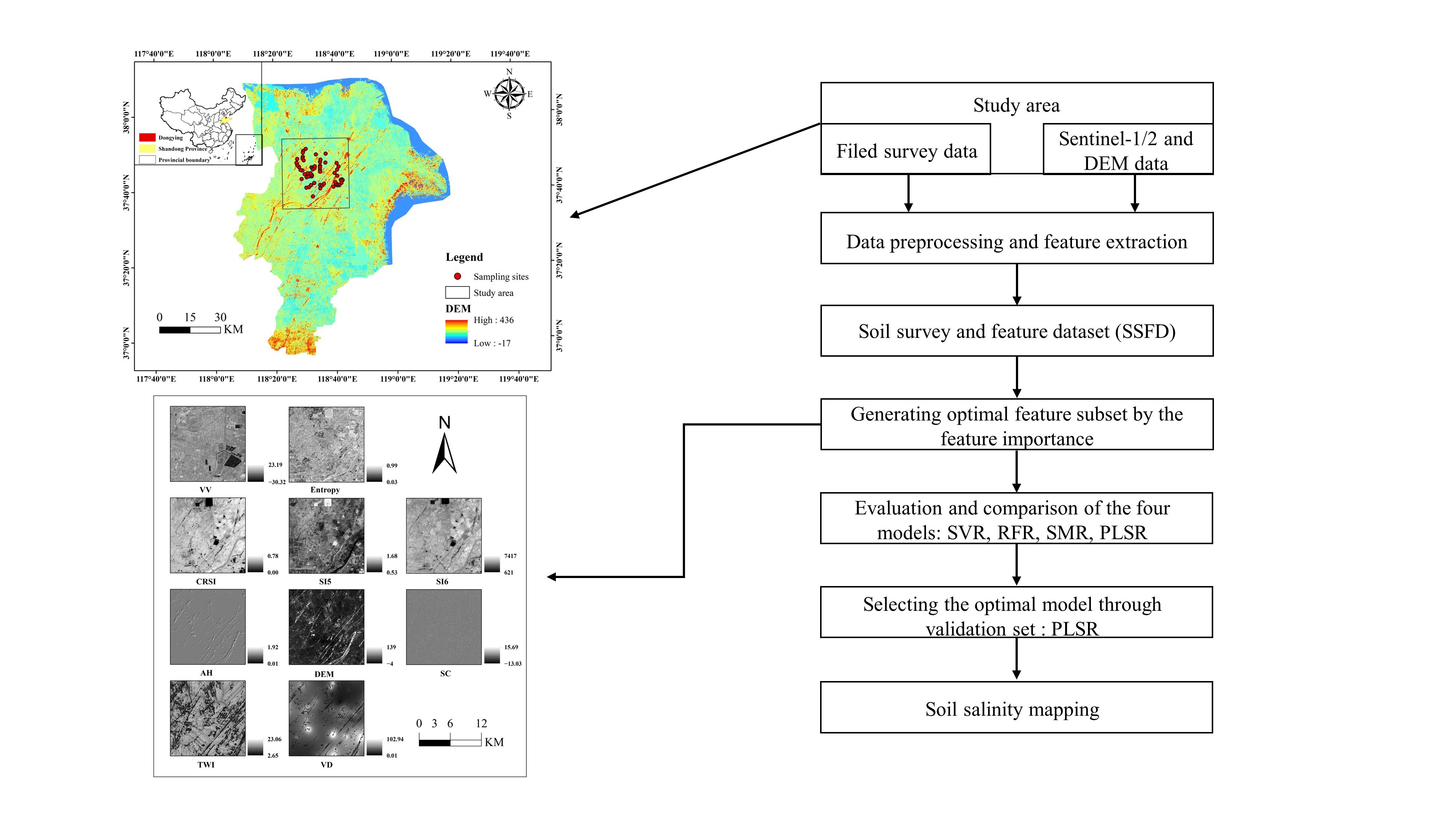
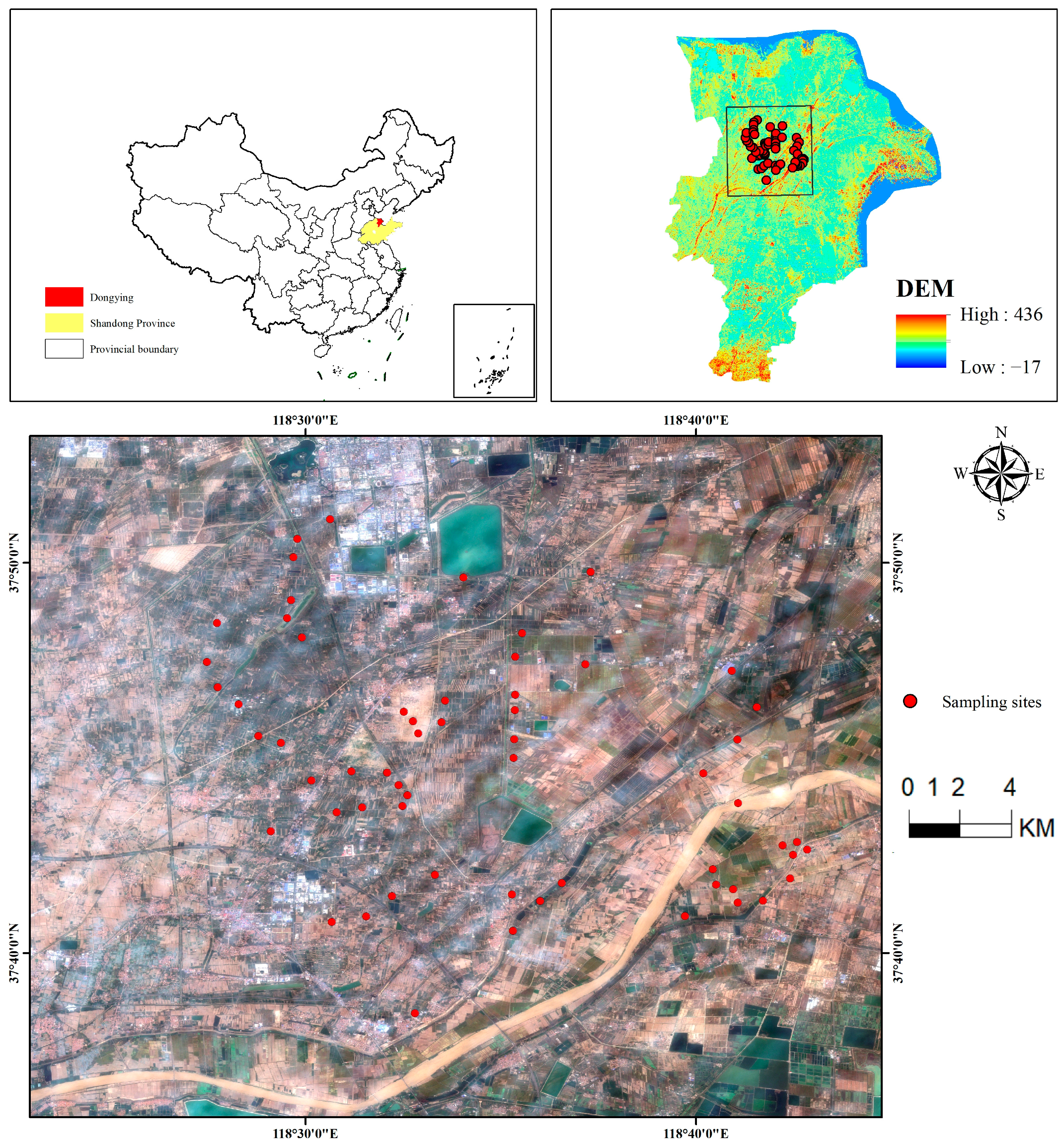
Generally, increasing numbers of scholars are using optical or radar data to retrieve soil salinity. However, few studies choose environmental variables from the perspective of soil genesis to monitor soil information in combination with optical or radar data. This research attempted to screen the optimal combination of variables based on the random forest method of feature importance, using environmental factors derived from DEM data and optical or radar indices derived from Sentinel-1/2 remote sensing imagery data to map the spatial distribution of soil salinization in Shandong Province, in combination with four machine learning algorithms. In this study, we compared and analyzed the most suitable model for this region among the four models and selected the optimal model to monitor and obtain soil salinization information. The proportion of salt-affected soil area was considered to provide scientific guidance for the environmental management and ecological protection of salinized soil in the area.

2. Materials and Methods

2.1. Study Area

Dongying is an important city in the Yellow River Delta, which is located in the north of Shandong Province, China (Figure 1), with a latitude of 36°55′N–38°10′N and a longitude of 118°07′E–119°10′E. The terrain of Dongying City inclines from southwest to northeast along the Yellow River. The highest elevation in the southwest is 28 m, and the lowest elevation in the northeast is 1 m. The highest elevation in the west is 11 m, and the lowest elevation in the east is 1 m. The region is a narrow strip from southwest to northeast with a longitudinal distance of 123 km from north to south and a leading transverse distance of 74 km, covering an area of 7923 km². It belongs to the warm, temperate, continental monsoon climate, and the weather here has four distinct seasons. The mean annual temperature is 12.8 °C, the mean annual evaporation is 1944 mm, and the mean annual rainfall is 555.9 mm. The rainfall varies significantly varies different years, making disasters such as floods and drought frequent. There are five categories of soil in this city: cinnamon soil, lime concretion black soil, moisture soil, saline soil and paddy soil. The saline soil accounts for 36% of the whole content of urban soil. The natural vegetation in Dongying City mainly includes reed, Suaeda salsa, thatch and artemisia [34].

2.2. Data and Preprocessing

2.2.1. Field Data

The design of the sampling sites comprehensively considers factors such as soil type, vegetation type, landscape characteristics and land use. First, we began to take soil samples in the field. In the process of field sampling, we randomly selected 60 sampling sites that were evenly distributed, with a sampling depth of 0–20 cm, from 9 October 2019 to 14 October 2019. All sampling sites were as far from roads and buildings as possible. Considering that there are some high-voltage lines in this area, we also had to keep away from the high-voltage lines when sampling. Therefore, when sampling in the field, for the sake of safety and convenience, some sampling points were selected in the same direction as the road. The shortest distance between adjacent sampling points was about 619 m, which is far enough to avoid the spatial dependence between samples. Then, we conducted laboratory analyses. The salt extraction experiment at the soil sampling site adopted the conductivity process. First, the soil sample were prepared. We took the soil sample back to the laboratory for natural air drying to remove impurities and to screen soil particles less than 2 mm. Then, we prepared a soil solution with a water/soil ratio of 5:1 by weighing 20 g of soil sample and 100 mL of deionized water, and the EC_1:5 values of the soil solution were measured by the electrical conductivity meter (the EC_1:5 values were extracted from the soil solution with a water/soil ratio of 5:1). Subsequently, the composition and content of the various ions in the soil were extracted using the conductivity method. Finally, we obtained the total salt content in the soil using a correlation model between soil salt content and electrical conductivity. The salinization was quantitatively assessed, using the EC values.

Before the experiment, we performed descriptive statistics on some soil characteristics at the sampling sites.

Table 1. Descriptive statistics of soil properties.

Soil Properties	Minimum	Maximum	Mean	Standard Deviation	Variance	Variable Coefficient/%
EC/(ds·m−1)	0.12	9.43	1.52	2.02	4.09	132.89
Salinity/(g·kg−1)	0.20	30.56	4.09	5.38	27.64	131.54
SMC/%	6.71	26.51	16.80	5.26	27.64	31.31
PH value	7.53	8.98	8.14	0.31	0.098	3.81

Note: EC is electric conductivity, ds/cm; SMC is soil moisture content, %.

describes the four soil characteristics, including soil salt content, EC value, soil moisture content and PH, based on the minimum, maximum, average, standard deviation and variable coefficient (CV). As can be seen from the table, the soil salt content in the whole sampling area varies greatly, ranging from 0.20 to 30.56 g/kg, with a CV value greater than 1. The EC value in the soil varies from 0.12 to 9.43 ds/m, while the CV is close to the soil salt content. The range of soil moisture content (SMC) shows little change, being 6.71~26.51%, while the CV value is 31.31%. The range of pH values is very small, ranging from 7.53 to 8.98, with a minimal CV value.

The table above lists the characteristic statistics of four soil properties, which are similar to the range of previous studies [3] and show that the sampling sites in this experiment are representative. According to the grading standard of [35], soil salinity can be classified into five grades: none, slightly, moderately, highly and extremely. According to the value range of the EC values, the soil salinization standard classification is as follows: non-saline, slightly saline, moderately saline, highly saline and extremely saline (

Table 2. Classification standard of soil salinity.

Salinity Class	EC (ds/m)	Proportion /%	Plant Response
Non-saline	<2	70.2	No salt damage to crops
Slightly	2~4	19.2	The yield of crops sensitive to salt may be affected
Moderately	4~8	8.5	The yield of salt-sensitive crops is affected, but it has little impact on salt-tolerant plants
Highly	8~16	2.1	Only salt-tolerant crops are harvested, but the yield is affected
Extremely	>16	0	Only a few salt-tolerant plants grow

).

The results show that approximately 70.2% of the sampling sites contain non-saline soil, 19.2% of sampling sites contain slightly saline soil, 8.5% of sampling sites contain moderately saline soil, 2.1% of sampling sites contain highly saline soil, and there is no extremely saline soil in the sampling area.

2.2.2. Sentinel-1 SAR Data

Sentinel-1 is composed of two polar-orbiting satellites, including Sentinel-1A and Sentinel-1B, which belong to active microwave remote sensing satellites. The sensors on the two satellites carry C-band synthetic aperture radar (SAR) instruments. Each satellite of Sentinel-1 provides active SAR data with a 12-day revisit period. In this study, the single look complex image (SLC) of Sentinel-1A satellites was acquired for radar parameters modeled from the European Space Agency (ESA) Data Hub. Specific parameters are given in

Table 3. Main parameters of Sentinel-1A data.

Parameter	Value	Parameter	Value
Date	8 October 2019	Processing level	Level 1
Polarization	VV, VH	Frequency	5.4 GHz
Relative orbit	69	Range pixel spacing	2.32 m
Orbit direction	Ascending	Azimuth pixel spacing	13.93 m
Mode	IW	Ground resolution (Range × Azimuth)	≈5 m × 20 m
File format	SAFE	Incidence angle	39.15°

.

The pre-processing of the downloaded Sentinel-1A SLC data was carried out on SNAP v8.0 software for orbit correction, radiometric calibration, multi-look processing and geographic correction. In the next step, the polarization decomposition parameters were acquired on POLSARPRO v5.1.3 software in the following two steps: polarization speckle filtering and H/A/a polarization decomposition. Finally, we obtained the following decomposition parameters using the H/A/a polarization decomposition method on POLSARPRO v5.1.3 software (

Table 4. H/A/a polarization decomposition parameters.

Feature Types	Description	Parameters	Processing
Original Backscatter features	Normalized backscatter coefficient	Sigma0_VV	SNAP
		Sigma0_VH	SNAP
Polarization decomposition parameter	Entropy	H	POLSARPRO
	Anisotropy	A	POLSARPRO
	Alpha	α	POLSARPRO
	Eigenvalue 1	L1	POLSARPRO
	Eigenvalue 2	L2	POLSARPRO
	H/A/Alpha Decomposition	Lambda, Delta, Delta1, Delta2, Alpha1, Alpha2, p1, p2, HA, H(1-A), (1-H) A	POLSARPRO

).

2.2.3. Sentinel-2 MSI Data

The multispectral instrument (MSI) on board the Sentinel satellites (2A and 2B) images the Earth’s surface from an altitude of 786 km in 13 spectral bands (VNIR and SWIR wavelengths), assuring a temporal resolution of less than 5 days. Compared with remote sensing images such as those of Landsat TM and ETM+ (with a revisit period of 16 days), Sentinel-2A has a higher spatial resolution, higher spectral resolution and a shorter revisit period. Its ground resolution in the visible light band can reach 10 m.

Table 5. Main parameters of Sentinel-2A data.

Parameter	Value	Parameter	Value
Date	19 October 2019	Processing level	Level-2A
Relative orbit	132	Cloud cover percentage	3.269213
Orbit direction	Descending	Resolution	10 m, 20 m, 60 m
File format	SAFE	Time resolution	10 d

shows the main parameters of Sentinel-2A.

This study selected the data of the Level-2A product, which had undergone radiometric calibration and atmospheric correction. Therefore, we did not need to carry out the pre-processing steps of radiometric calibration and atmospheric correction, but only needed to carry out resampling, format conversion, layer stacking and image clipping. First, we imported Sentinel-2 original image data into SNAP V8.0 software. Next, we resampled the image to 10 m resolution, based on the visible light band B2 (the resolution is 10 m) and we then exported the data to an ENVI format file. In the next step, we used ENVI v5.3 software for layer stacking and clipping. Finally, the vegetation indices and salinity indices were calculated according to the following formula, as shown in

Table 6. Vegetation index and salinity index.

Feature Types	Parameters	Formulations	Reference
Vegetation index	NSI	$\frac{F_{SWIR1}-F_{SWIR2}}{F_{SWIR1}-F_{NIR}}$	[28]
	VSSI	${2\ast F}_G-5\ast \left(F_R+F_{NIR}\right)$	[36]
	NDSI	$\frac{F_R-F_{NIR}}{F_R+F_{NIR}}$	[37]
	SR	$\frac{F_G-F_R}{F_B+F_R}$	[38]
	CRSI	$\sqrt{\frac{F_{NIR}\ast F_R-F_G\ast F_B}{F_{NIR}\ast F_R+F_G\ast F_B}}$	[39]
	BI	$\sqrt{{F_R}^2+{F_{NIR}}^2}$	[37]
Salinity index	SI1	$\sqrt{\left(F_R\ast F_G\right)}$	[39]
	SI2	$\sqrt{\left(F_R\ast F_B\right)}$	[29]
	SI3	$\sqrt{\left({F_R}^2\ast {F_G}^2\right)}$	[29]
	SI4	$\frac{F_{NIR}\ast F_{SWIR1}-{F_{SWIR1}}^2}{F_{NIR}}$	[38]
	SI5	$\frac{F_B}{F_R}$	[38]
	SI6	$\frac{F_R\ast F_{NIR}}{F_G}$	[38]

.

2.2.4. ASTER GDEM

Environmental variables, such as parent material, climate, topography and biology, play a crucial role in the process of the formation of soil salinization, due to the complex causes of soil salinization. To comprehensively consider the influencing factors of soil salinization, we selected topographic factors derived from the DEM data for the inversion of soil salinization. Finally, we selected 18 topographic factors as the independent variables to retrieve the soil salinity. The ASTER GDEM V2 data have a resolution of 30 m. The pre-processing of the downloaded DEM data was carried out on ArcGIS software by image mosaicking, image cropping and projection, while the subsequent processing of the pre-processed data was carried out using the SAGA software to obtain 14 basic terrain parameters. Before terrain analysis in SAGA, it is necessary to fill sinks. The plane curvature, profile curvature, fluctuation and roughness are calculated from the projected 30 m digital elevation model using the ArcGIS v10.2.2 software. Specific indices are given in

Table 7. Characteristic variables derived from DEM.

Feature Types	Description	Parameters	Reference
Topographic index	Digital elevation model	DEM	[26]
	Analytical hill-shading	AH	[24]
	Aspect	AS	[40]
	Slope	S	[40]
	Longitudinal curvature	LC	[40]
	Tangential curvature	TC	[40]
	Channel network distance	CND	[41]
	Channel network base lever	CNBL	[41]
	Total catchment area	TCA	[41]
	Topographic wetness index	TWI	[24]
	LS-factor	LSF	[24]
	Convergence index	CI	[24]
	Relative slope position	RSP	[24]
	Valley depth	VD	[42]
	Roughness of surface	RS	[40]
	Plane curvature	SC	[40]
	Profile curvature	PC	[40]

.

2.3. Methods

To find the relationship between all influencing parameters and soil conductivity, four methods were used to model soil salinity research. Finally, we compared the performance of the four models by comparing the R² and RMSE of the experimental results, and chose the optical model to map soil salinity.

2.3.1. Stepwise Multiple Regression

Stepwise multiple regression (SMR) is one of the multiple linear regression models that can better eliminate unimportant parameters and reduce high collinearity in variables. During the regression process, the independent variables that passed the F-test and T-test were sequentially imported into the model one by one. Since imported new variables cause the old variables to no longer be significant, the model automatically eliminates the old variables to obtain the optimal variable set for modeling. The standard methods of stepwise regression are the forward method and the backward method. Here, we use the forward method, the variables of which are added from few to many, one by one, until there are no variables to add. Its steps are as follows:

• Establish the single regression equation of the measured value Y and the values of the modeling parameters $X_1,X_2,\cdots {,X}_n$, respectively:

  $$Y={\beta }_0+{\beta }_i{X}_i+\epsilon ,i=\mathrm{1,2},\cdots ,n$$

  (1)

Calculate the values of the F-test statistic of the regression coefficient of each variable $X_i$, which are $F_1^{\left(1\right)},\cdots {,F}_n^{\left(1\right)}$. We selected the maximum value $F_{i1}^{\left(1\right)}$:

$$F_{i1}^{\left(1\right)}=\max \left\{F_1^{\left(1\right)},\cdots F_n^{\left(1\right)}\right\}$$

(2)

At a given level of significance $\alpha$, its corresponding critical value is $F^{\left(1\right)}$. If $F_{i1}^{\left(1\right)}>F^{\left(1\right)}$, $X_{i1}$ is selected for modeling.

2.

Establish the binary regression model between Y and the independent variables ${\{X}_{i1}{,X}_1\},\cdots ,{\{X}_{i1},X_{i1-1}\},{\{X}_{i1},X_{i1+1}\},\cdots ,{\{X}_{i1},X_n\}$.

After removing variable ${\mathrm{X}}_{\mathrm{i}1}$ introduced above, the remaining n − 1 independent variable can be used to calculate the values of the F-test statistic, which are $F_1^{\left(2\right)},\cdots ,F_n^{\left(2\right)}$, and to remove the largest $F_{i2}^{\left(2\right)}$, that is:

$$F_{i2}^{\left(2\right)}=\max \left\{F_1^{\left(2\right)},\cdots {,F_{i1-1}^{\left(2\right)},F_{i1+1}^{\left(2\right)},\cdots ,F}_n^{\left(2\right)}\right\}$$

(3)

Record the critical value $F^{\left(2\right)}$; if $F_{i2}^{\left(2\right)}>F^{\left(2\right)}$, $X_{i2}$ will be selected for the model; otherwise, the model will terminate the selection of variables.

3.

Continue to perform the regression operation between Y and variable set ${\{X}_{i1},X_{i2},X_k\}$, and repeat the process in 2.

The stepwise regression analysis can be carried out using the SPSS v25 software and MATLAB software. In this study, we selected the stepwise function of the MATLAB software to perform stepwise regression operations with the soil conductivity Y as the dependent variable, seventeen SAR polarization decomposition parameters, two backscattering coefficients, thirteen salinity vegetation indices and eighteen topographic factors as the independent variables of stepwise regression.

2.3.2. Support Vector Regression

Support vector regression (SVR) is a branch of SVM based on statistical learning theory. Compared with general linear regression, SVR will calculate the loss only when the absolute value of the difference between the predicted value f(x) and the measured value y is greater than the threshold value $\epsilon$. Any value below the threshold $\epsilon$ is acceptable. SVR transforms data into a high-dimensional feature space through a non-linear transformation to establish a linear model and fit the regression model, in order to solve the high-dimensional problems of “many discrete values” and “over learning” [43]. The cost parameter C and kernel parameter γ are the main parameters that can affect the performance of the model. Parameter C directly affects the stability of the model. When the value of parameter C is higher, the model is easier to overfit; otherwise, the model is more likely to underfit. When the value of parameter γ is larger, fewer support vectors can affect the speed of the model; otherwise, there are more support vectors [44]. There are many versions of SVR, such as segmentation algorithms, decomposition algorithms, C-SVR, V-SVR and sequential minimal optimization (SMO) [45]. In this study, we used the SMO method for soil salinity mapping, because it can derive a high-performance model [46]. We can use the following formula to express the SMO-SVR model:

$$f\left(x\right)=\sum _{i=1}^m\left(\widehat{{\alpha }_i}{-\alpha }_i\right)k\left(x_i^{T}x\right)+b$$

(4)

where $\widehat{{\alpha }_i}{,\alpha }_i$ represents the Lagrange multiplier and $k\left(x_i^{T}x\right)$ is the RBF kernel function.

The research used MATLAB2016a software and the software package LIBSVM developed by Professor Lin of Taiwan University to establish and predict the support vector regression model. For the problem of how to select the optimal parameters of the SVR, grid search (GS), genetic algorithm (GA) and particle swarm optimization (PSO) are common methods for parameter optimization. In this study, the form of SVM we used is ε-SVR, which strives to find a model with minimum RMSE. In this study, we used the PSO method to find the best values for parameters C and γ.

2.3.3. Random Forests

Random forest (RF) is an integrated learning algorithm that Breiman combined with classification trees in 2001. This algorithm has the advantages of non-linear mining ability, good anti-noise ability, a data distribution that cannot meet any assumptions, strong adaptability to datasets and fast training speed [47]. First, the RF model uses the bootstrap aggregation algorithm to randomly sample the original training set into n training subsets. Then, it can randomly select K features (K < n) from each training set. In the next step, the model can build m sub-decision trees and calculate their prediction results repeatedly, according to these K features. Finally, the model can vote on the classification model and select the model with the highest number of votes as the final decision [8]. The specific process can be seen in Figure 2.

From the above figure, we can see that the random forest model usually has three key parameters, including the number of decision trees (NumTrees), number of features selected randomly from each node of each tree (MaxFeatures) and minimum number of observations per leaf (MinLeaf) [48]. In this study, we use the TreeBagger function that comes with MATLAB. It requires users to define the NumTrees and MinLeaf parameters. Generally, by default, MinLeaf should be set to 5 for regression and used as a classification when it is 1. However, it is not certain whether the default value of NumTree produces a reliable result, so we need to traverse to obtain the optimal value of NumTrees. In this study, the optimal outcome is 200. We need to eliminate the interference of some unimportant parameters and measure the importance of the variables by using the feature importance of the RF model, due to the large number of parameters in this study. The basic idea is that under the single decision tree t, we recorded each sample of Out-of-Bag (OOB) as ${OOB}_t$ and its corresponding error as $err{OOB}_t$. Then, the model can randomly arrange the value of $X^j$ in ${OOB}_t$ to obtain a new set of disturbance samples $\widetilde{{OOB}_t^j}$ and can calculate its error $err\widetilde{{OOB}_t^j}$. The feature importance of $X^j$ is to calculate the average reduction of all decision trees, based on the error reduction of $err\widetilde{{OOB}_t^j}$ and $err{OOB}_t$ on the single decision tree [8,33]. The formula is as follows:

$$VI\left(X^j\right)=\frac{1}{ntree}\sum _{t=1}^{ntree}\left(err\widetilde{{OOB}_t^j}-err{OOB}_t\right)$$

(5)

where t represents the single decision tree and ntree is the number of trees in RF.

It can be seen from the formula that, when there is no difference between $err\widetilde{{OOB}_t^j}$ and $err{OOB}_t$, the input variable has no predictive value, which means that the larger the VI, the more critical its corresponding variable.

2.3.4. Partial Least Squares Regression

Partial least squares regression (PLSR) can be used to study the relationship between two matrices. The model has many advantages, such as being able to evaluate the relationship between multiple independent variables and multiple dependent variables, and a better model being obtained when there are multiple collinearities between independent variables [49]. At present, the PLSR model has been widely used in the remote sensing monitoring of soil components, such as soil salt content [50], soil nutrients [51], soil organic carbon [52] and soil moisture content [53]. The PLSR model can re-project the prediction matrix X and observation matrix Y into a new space to establish a new regression model, which can significantly reduce noise. It can screen some information with a strong explanatory ability and can eliminate the influence of some useless information [54]. The general multivariate underlying equation is as below:

$$X=T{P}^T+E$$

(6)

$$Y=U{Q}^T+F$$

(7)

where Y is an n × p response matrix; X is the modeling matrix of n × m; T is the projection of X, also known as the factor matrix; U is the projection of Y; P and Q are the orthogonal load matrices; and E and F represent the error.

Based on the above estimation factors T and U and the load matrices P and Q, a linear model of Y and X can finally be established by the PLSR model. The equation is as follows:

$$Y=Xb+e$$

(8)

where b is the coefficient of the PLSR model and e is the error vector.

This study discussed the feasibility of using the PLSR model to establish the quantitative relationship between soil salt content and influencing factors.

2.4. Accuracy Assessment

This study used the K-fold cross-validation (K-CV) method to verify the accuracy. The K-CV model has excellent guiding and validation significance for machine learning. The basic idea is to divide the sampling data into training sets and validation sets, which is a standard method in cross-validation. Taghizadeh-Mehrjardi et al. [55] suggested that the k value should be set as five, which has the advantages of unbiased estimation, stability, and reliability for the calculated results. At the same time, the verification process requires repeated iterations, rather than a single round of training and verification. This validation method is more suitable for smaller datasets. In this study, the training set was randomly divided into 5 subsets, in which 4/5 observed values were used for model training and 1/5 measured values for model verification. This study used the root-mean-square error (RMSE) and determination coefficient (R²) to determine the final accuracy. The formula is as below:

$$RMSE=\sqrt{\frac{1}{n}\sum _{i=1}^n{\left(Y_i-{\overline{Y}}_i\right)}^2}$$

(9)

$$R^2=1-\frac{{\sum }_{i=1}^n{\left(y_i-f_i\right)}^2}{{\sum }_{i=1}^n{\left(y_i-\overline{y}\right)}^2}$$

(10)

where $y_i$ is the actual dataset; $f_i$ is the predicted dataset; and $\overline{y}$ is the average value. When R² is approaching one while RMSE is approaching zero, the model tends to be optimal.

2.5. Soil Salinity Retrieval

This section mainly describes the method and experimental procedure for soil salinity mapping. First, we needed to obtain various types of data, including remote sensing image data, DEM data and ground data. Then, we needed to pre-process the data to extract the impact factors of various types corresponding to the sampling points. In the next step, we established a geographic database of the EC values and the used factors. Then, we divided the original data into the training dataset and the testing dataset, using the K-CV method. The four models selected in this paper were used to model the training set data by using MATLAB software. Subsequently, we obtained the precision performance of the four models. Finally, the best model was selected to map soil salinity and summarize the distribution characteristics. The whole workflow is given in Figure 3.

3. Results

3.1. Feature Selection

In this experiment, we selected approximately 50 parameters as independent variables, including radar parameters, salinity indices, vegetation indices and terrain factors. However, not every parameter plays a critical role in the accuracy of soil salinity. Some parameters may have noise, leading to information redundancy and overfitting. Such parameters will reduce the prediction accuracy of the regression model. Therefore, they are redundant and need to be eliminated [17]. To address this problem, this study used the feature importance of the RF model to screen some crucial parameters and remove some less important parameters. The algorithm can calculate the importance of the independent variables in relation to the dependent variables and the relative effects among all variables [56]. The operation platform of this experiment is the MATLAB environment. We inputted the selected variables into the RF model using the TreeBagger function from MATLAB2016a to obtain the relative importance of each parameter and sort them in descending order. In this study, due to the importance between the 10th and 11th features having dropped significantly, we chose the top 10 features in the experiment and eliminated other features that were not significant. Through calculation, the radio of the cumulative importance value of the top 10 features to the cumulative importance value of all features exceeded 0.9 [33]. Therefore, the top ten parameters with the greatest importance were selected in this research, and are summarized in Figure 4.

The higher the variable importance (VI), the closer the relationship between this characteristic and soil EC. Therefore, the characteristics closely related to the EC value can be obtained for modeling, according to the VI value.

3.2. Visual Map of All Features

The ten feature parameters screened by the above model were used to display the visualization of the grey values in the ArcGIS v10.2.2 software. The contrast value of the pixels can reveal the response of soil salt characteristics [9]. The polarization decomposition parameter, including entropy, backscattering coefficient including VV, and optical indices including CRSI, SI5 and SI6, have more spatial and texture information and more visual information. At the same time, the visual information of the remaining terrain factors is not too rich compared with the ten features in the study area (Figure 5).

3.3. The Performance of the Models

To verify the performance of the four methods used here, we substitute the testing set into the four regression models of machine learning to predict their accuracy and compare their performance.

3.3.1. Determination of Model Parameters

Compared with the other models, the SVR model needs to determine the optimal values of parameters C and gamma. We set the initial value of the following parameters: parameter C1 is 2, parameter C2 is 0.6, the termination algebra is 200 and the population number is 20. This experiment uses the PSO method to determine the optimal value.

The experimental results show that the best parameter C is 7.802, and the best parameter gamma is 1.859 for the SVR model. Finally, when the parameter CVMSE tends to be stable, the value is 0.204.

According to the experimental results, the optimal number of the parameter Ntrees in the RF model is 200 for the random forest model.

3.3.2. Regression Modeling

The divided training set and the testing set were substituted into the four models for training. Figure 6 shows the scatter plot and model accuracy of the four models.

3.3.3. Performance Comparison of Four Models

For instances when we use only remote sensing data (optical and radar image data) or use only topographic factors extracted from DEM data to obtain the soil salinity information of the region, the performances of the validation set of these four models are shown in

Table 8. Performance of the four models using only remote sensing data or DEM.

Model	Remote Sensing Image Features		Topographic Factors
	R2	RMSE	R2	RMSE
SMR	0.47	1.63	0.13	1.78
SVR	0.25	0.32	0.18	0.38
RFR	0.59	1.34	0.15	1.71
PLSR	0.55	1.35	0.14	1.81

.

Then, we put all features extracted from remote sensing data and DEM data into these four models for training, and the accuracy of these four models was significantly improved. The performances of the four methods for soil salinity prediction are summarized in

Table 9. Performance of the four models in soil salinity retrieval.

Model	Training Set		Testing Set
	R2	RMSE	R2	RMSE
SMR	0.66	1.26	0.51	1.38
SVR	0.43	0.27	0.40	0.29
RFR	0.76	1.21	0.63	1.33
PLSR	0.70	1.16	0.66	1.30

. The lowest RMSE and the highest R² represent the highest fitting performance. In the testing set of the four models in this paper, the R² of the PLSR model is the highest, with a value of 0.66, followed by the RF model, with an R² of 0.63, and the stepwise multiple regression model (SMR), with an R² of 0.51. Compared with the other methods, the R² of the support vector regression model (SVR) is the lowest, with an R² of 0.40. However, SVR has the lowest RMSE (0.29), and SMR has the highest RMSE (1.38), followed by the RF model (RMSE = 1.33). The RMSE of the testing set for the PLSR model is 1.30, which is slightly more significant than that of the training set (RMSE = 1.16). Compared with the other models, the PLSR model has a good effect and has the highest fit (R² = 0.66) among the four models in this experiment.

According to the above comparison, we comprehensively considered the R² and the RMSE to select the optimal model for soil salinity mapping. Finally, we selected the PLSR model to conduct the follow-up study on the distribution of soil salinization. Here, we mainly introduce some basic parameters of the PLSR model. The results of the partial least squares regression model (Figure 7) indicate that among the regression coefficients between soil salinity and various parameters, band 3 (CRSI) makes the highest contribution to the estimation of soil salinity, followed by band 5 (SI5), band 10 (VD), band 7 (DEM), band 8 (SC) and band 1 (VV). The remaining bands make low contributions to the estimation of soil salinity.

Finally, according to the results of the PLSR model, the regression equations between the soil salt content and various variables can be obtained, to create a spatial distribution map of the soil salinity of the region. The corresponding relationships between soil salinity and each variable are shown in

Table 10. Regression equations of the PLSR model.

Model No.	Model in EC (ds/m)	R2	RMSE
Standard data equation	Y = −0.054 × VV − 0.029 × Entropy − 0.421 × CRSI + 0.062 × SI5 − 0.245 × SI6 − 0.081 × AH + 0.10 × DEM + 0.087 × SC − 0.061 × TWI − 0.157 × VD	0.66	1.30
Original data equation	Y = 13.733 − 0.054 × VV − 0.506 × Entropy − 12.669 × CRSI + 1.519 × SI5 − 0.002 × SI6 − 2.708 × AH + 0.027 × DEM + 0.372 × SC − 0.037 × TWI − 0.051 × VD

.

3.4. Soil Salinity Mapping

From the above analysis, we can conclude that the PLSR model is the best method. Therefore, we selected this model to obtain spatial information on soil salinization. First, we input the ten selected features into the trained PLSR model to calculate the soil salinity of each pixel, and generate the spatial distribution map of soil salt using ArcGIS v10.2.2 software (Figure 8). The white layer in Figure 8 represents urban buildings and villages.

The statistics regarding the percentage of the salinization degree are shown in

Table 11. Percentage of coverage of various degrees of salinization.

Classified Statistics	Non-Saline	Slightly	Moderately	Highly	Extremely
Proportion/%	64.2	29.2	6.2	0.4	0

. The proportion was calculated based on the proportion of pixels of each salinization degree compared with all pixels in the whole study area. It is reflected in the classified map of the salinization degree of the Yellow River Delta and the statistics in Table 10, that the study area is mainly non-saline soil, which covers more than half of the study area, distributed primarily in the east of the study area, accounting for 64.2% of the total area. The area of slight salinization is distributed in the west and north, accounting for 29.2% of the area. The area of moderate salinization is scattered across the study area, accounting for 6.2% of the total area. Severe salinization is only distributed in the southeast and north of the study area and some rivers, accounting for only 0.4% of the study area, being only a minor proportion. There is no extreme salinization in the study area. The proportion of each salinization area is consistent with the sample data. The results also indicate that from the geographical location, the degree of soil salinization gradually increases from east to west, being the most severe along the water body to the inland edge area. Due to the low terrain and shallow groundwater, the soil salinity in the estuary area is high. In addition, the degree of soil salinization along the Yellow River and the water surface of the reservoir is generally severe, generally within the range of 8 to 16 ds/m; on the contrary, due to the high terrain, the soil salt content in the northeast of the study area is low, generally being within the range of 0~2 ds/m. The intrusion of saline water causes soil salinization. The overall classification accuracy of the testing set is 85.71%, and the kappa coefficient is 0.58, which is an acceptable result. In the field measurements, even if we take some steps to calibrate the measurement results, including repeated measurements and careful sampling, errors will always also occur.

4. Discussion

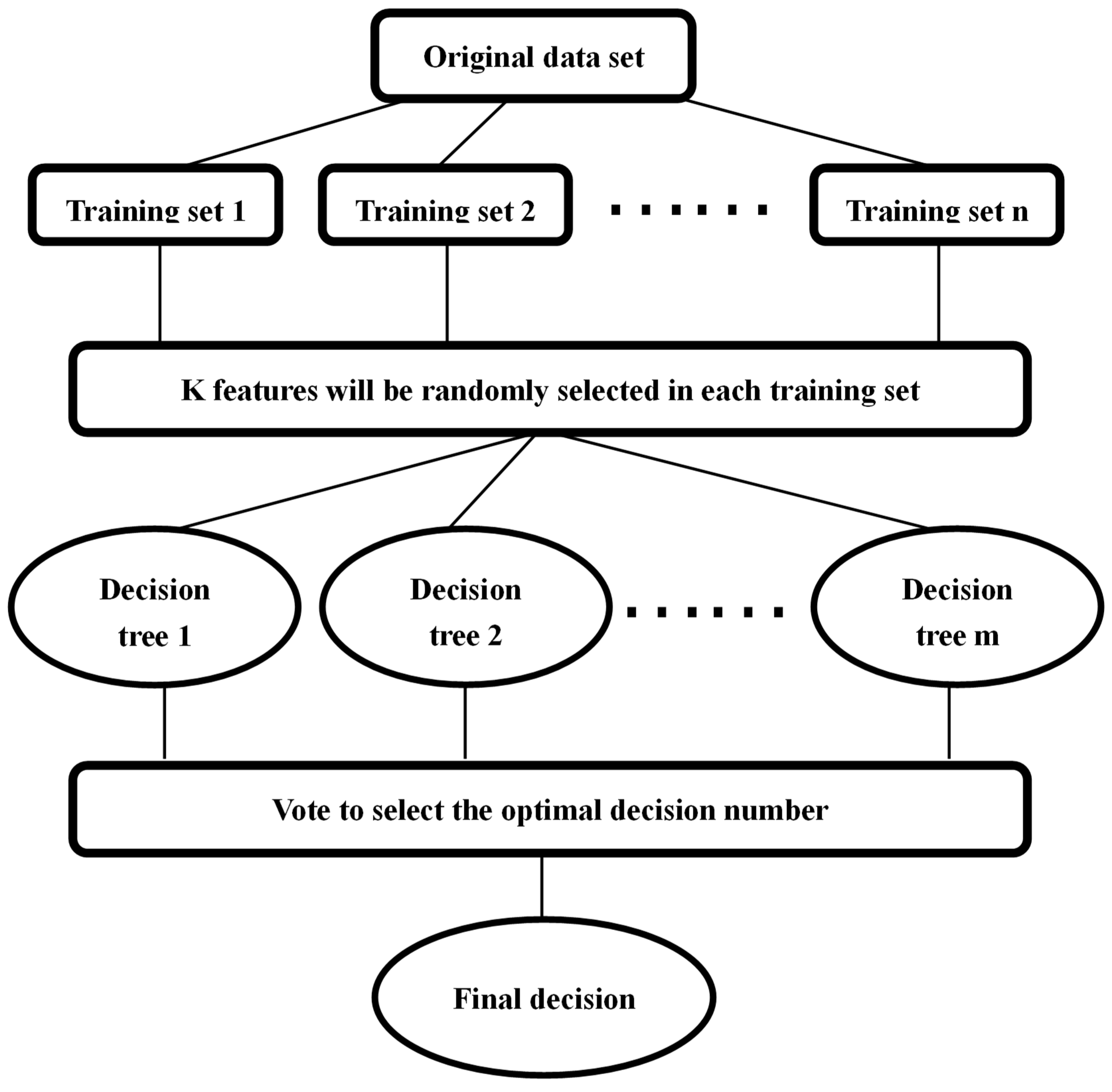
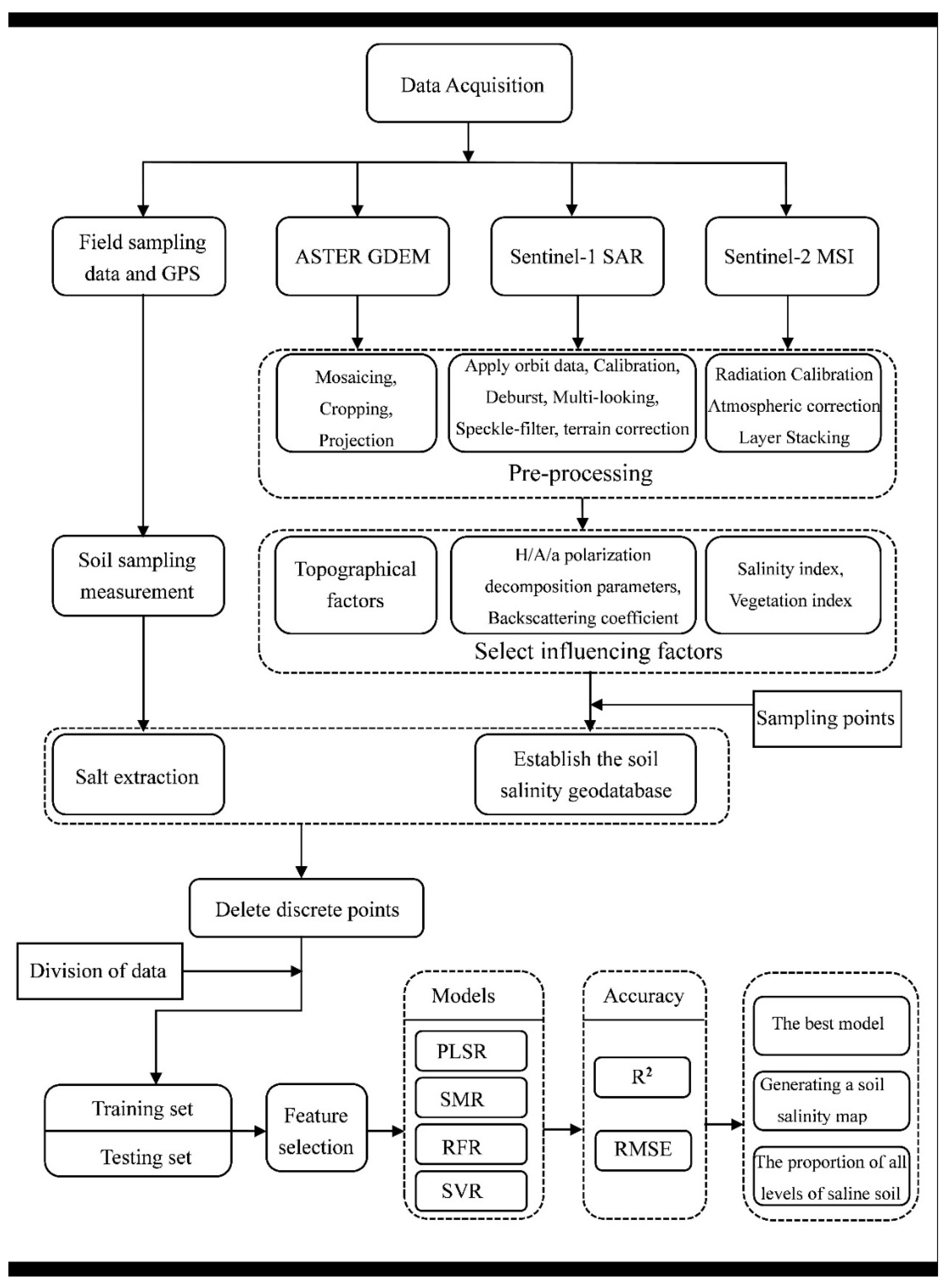
Soil salinization is a global environmental threat to ecosystem balance and agricultural production. Therefore, it is critical to monitor soil salinization in vulnerable areas. In this study, we used remote sensing data and topographic factors to obtain soil salinity information. Radar data can penetrate the Earth’s surface and play a particular role in monitoring soil salinity. The topographic factors were selected in this paper, due to terrain being one of the factors affecting soil formation. This experiment solved this problem well, by obtaining the soil salinization information based on the characteristic variables derived from Sentinel-1/2 and DEM data, using four regression methods for analysis. The experiment combined the advantages of topographic factors and remote sensing data, which can be used to screen the most suitable and influential characteristic parameters in this area and select the optimal model for regression analysis to create a spatial distribution map of soil salinization in this area. As a part of this study, we used the feature importance of the RF model to screen feature parameters. The method can demonstrate the influence of a single feature and the feature importance among variables. The results also show that the RF method is a good option for feature screening. The results obtained in this research are summarized and presented in detail in the following sections:

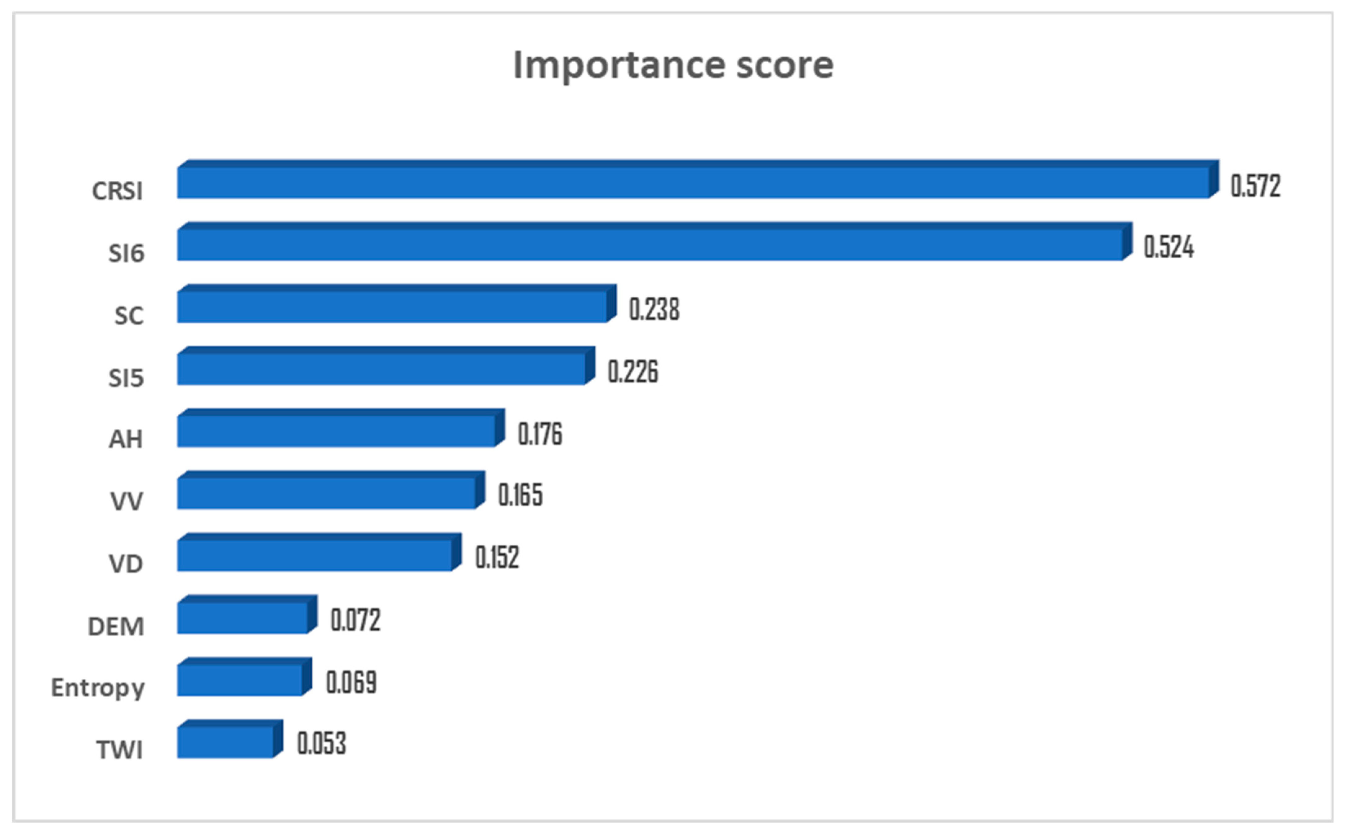
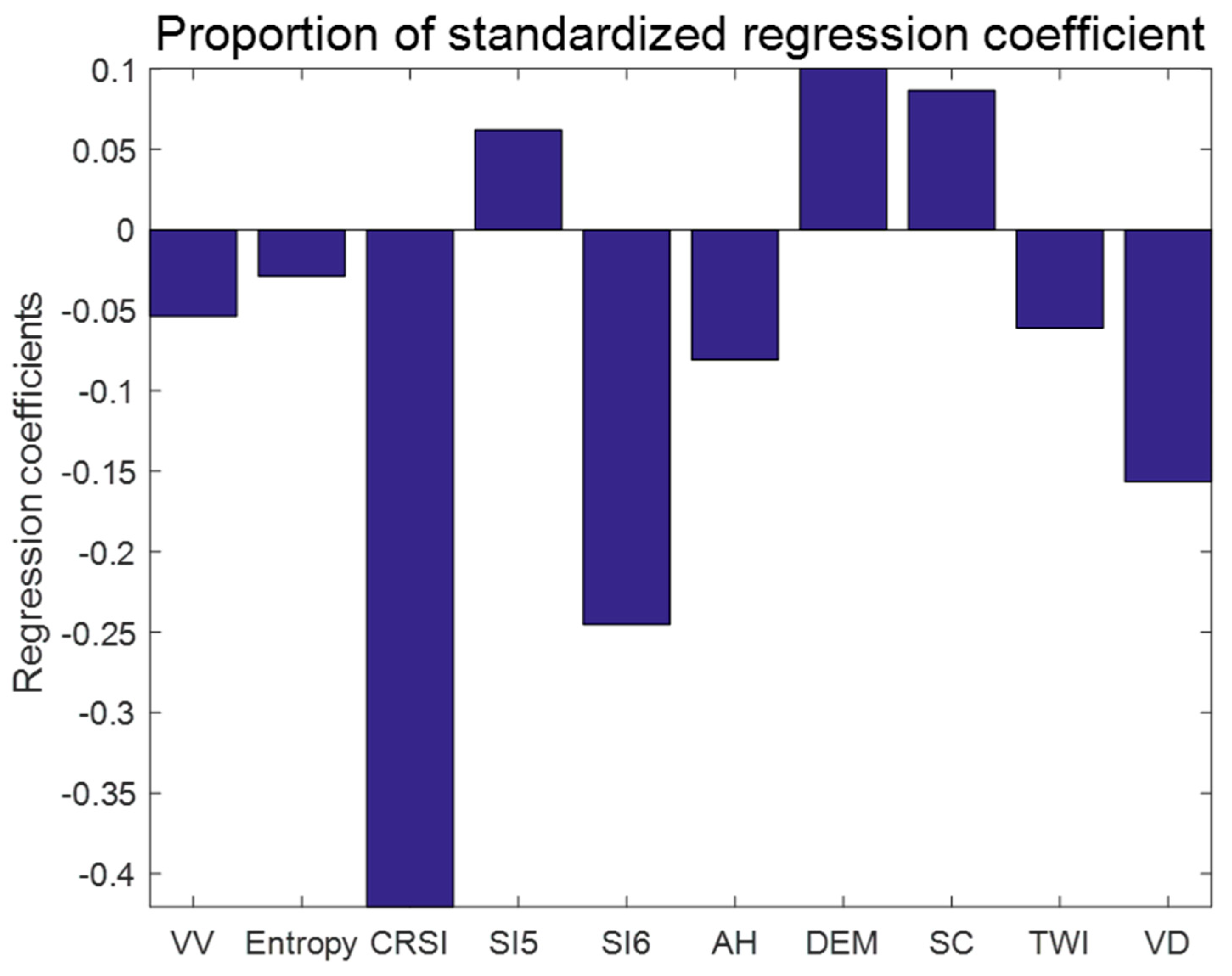
In general, soil salinization is affected by many factors, including terrain, climate, biology and parent material. There are many interference items for soil salinity mapping [8]. The experimental results also prove this view. For example, among all the radar parameters decomposed, only VV and entropy are selected as the selected feature variables, and they are also low in the feature importance ranking of the RF model. Among the ten features selected, the VV (0.165) is sixth in the sorting, and the entropy (0.069) is ninth. The correlation coefficients of the PLSR model also prove that the effect of the radar parameters on the model might not be ideal. In the existing studies, most of them only consider remote sensing image data or DEM data to retrieve the soil salt content [27,57]. For example, Zhang [9] achieved good results in retrieving soil salinity using 10 radar remote sensing features extracted from Sentinel-1 SAR image data. 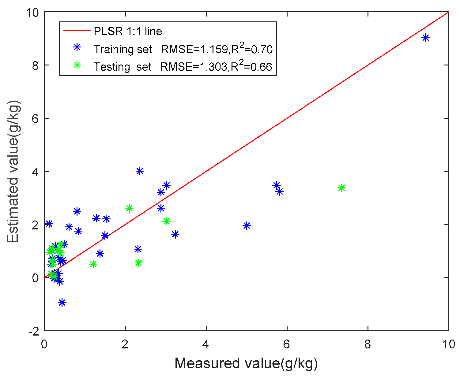Vermeulen [58] observed that there was great potential to monitor the accumulation of salt in irrigation areas using DEM and its derivatives, combined with four machine learning algorithms. However, in this paper, the accuracy of the four models were not ideal when only considering remote sensing image features or terrain factors for predicting soil salt content. Therefore, this paper used remote sensing image characteristics and topographic factors to retrieve the soil salt content in the study area. The results showed that the accuracy of the four models in this paper were significantly improved when all these factors were considered to predict the soil salt content, and that the best one was the PLSR model (R² = 0.66, RMSE = 1.30). Therefore, it is suggested that various factors are comprehensively considered to invert the soil salinity in order to obtain a model with a higher performance.

It can be seen from the importance analysis of the screened characteristic parameters in Figure 4 that the CRSI is the parameter with the most significant influence, followed by the salinity index SI6. The topographic factors and radar-derived products have little influence on soil salinity in this area. This result indicates that the parameters derived from the optical data are the most suitable factors for soil salinity modeling in the local area, which confirms some of the above views (it is difficult to monitor the soil salinity using only the radar data).

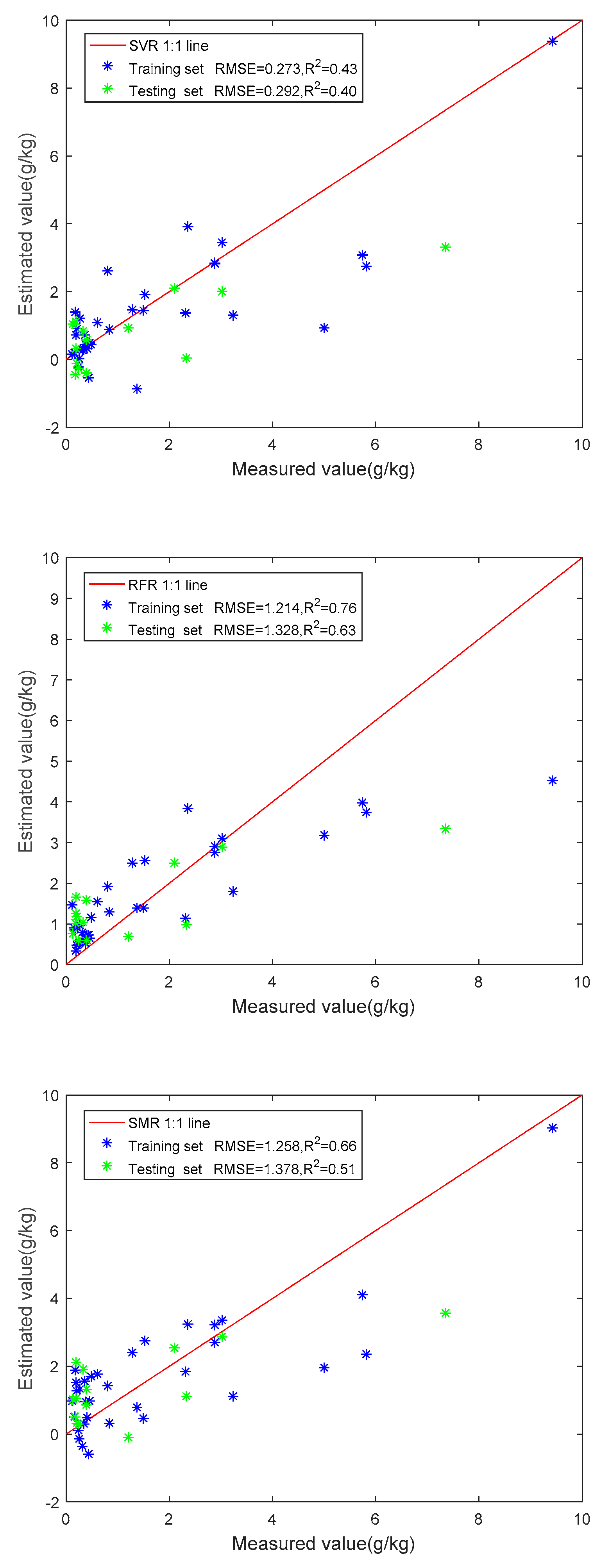
In this study, four regression models (SMR, SVR, RFR and PLSR) were used to monitor soil salinity, and they have been widely used to obtain information on soil salinity. It should be noted from the results of this study that the testing set of the PLSR model has the highest accuracy (R² = 0.66, RMSE = 1.30), and is the most suitable model for soil salt inversion in this region. Compared with the PLSR model, the other three models have a lower accuracy: the RFR model (R² = 0.63, RMSE = 1.33), the SMR model (R² = 0.51, RMSE = 1.38) and the SVR model with the lowest accuracy (R² = 0.40, RMSE = 0.29). The results obtained show that the R² of the training set of the RFR model reaches 0.76. The performance of the testing set of the RFR model is low (R² = 0.63), with a lower accuracy than the testing set of the PLSR model (R² = 0.66). The results indicate that the models in this experiment have a certain degree of overfitting, which is caused by the relatively small data sample.

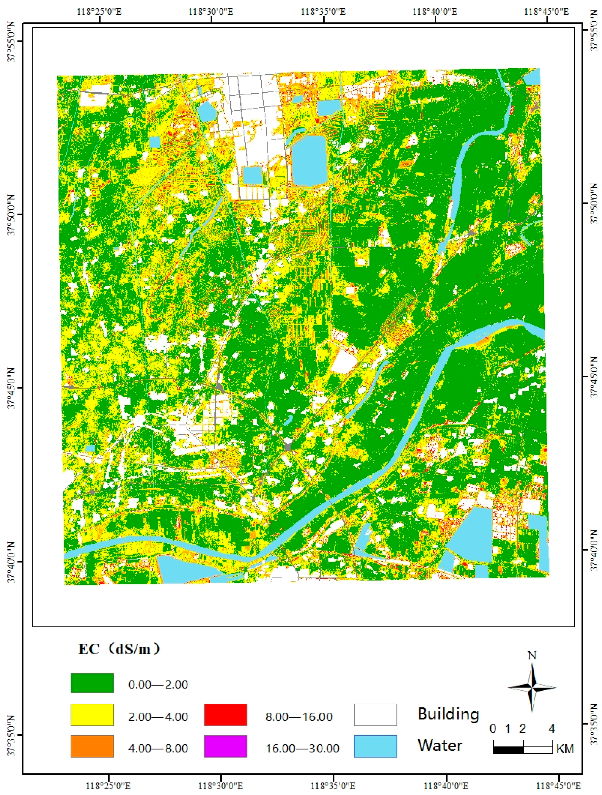
It can be seen from the salinization distribution map in the study area that the non-salinity soil is mainly distributed in the eastern part of the region, accounting for 64.2% of the area, representing the largest percentage. Soil with slight salinization was distributed in the west and north, accounting for 29.2% of the area. Soil with moderate salinization was scattered across the study area, accounting for 6.2% of the total area. Only a small amount of soil with severe salinization was distributed in the southeast and north, accounting for only 0.4% of the area. There was no soil with severe salinization in the study area. The proportion of each salinization degree was consistent with the sample data and the reference data. It can also be seen that the areas with high-salinization soil are mainly distributed around the residential areas and the water bodies, and are caused by low topography and shallow groundwater. Due to high topography, the soil salt content in the northeast region of the map is low.

Finally, the results indicate that more accurate models and spatial maps of soil salinity could be generated by combining the topographic factors selected from the perspective of soil genetics with optical or radar data. The results also show that machine learning methods are an effective tool for obtaining information on soil composition.

5. Conclusions

In this study, four methods (SR, SVR, RF and PLSR) were used to predict the spatial distribution of surface soil salt in this region by using topographic factors, vegetation indices, salinity indices and polarization decomposition parameters. To solve the problem of feature redundancy in the process of modeling, this study adopted the feature importance of the RF model to screen all features to reduce feature redundancy and select more effective feature variables. The results show that the CRSI index contributed the most, which was consistent with other findings, indicating that it was feasible to use the feature importance of the RF model to screen features. The results show that the PLSR model has a better performance than the other three models (SR, SVM and RF), and it can describe the local variation in soil salinity in more detail. The prediction accuracy of the PLSR method was the highest in the testing set, with an R² of 0.66 and RMSE of 1.30 g/kg, indicating that the PLSR model is feasible for predicting soil salinity information. According to the soil salt distribution map, the results in terms of soil salt inversion are consistent with the existing data. The level of soil salt near water bodies and tidal flats is higher, and in woodland and farmland it is lower. The inversion of soil salinity with high precision is still restricted by many factors, such as the number of samples, the climate data during the sampling period, the accuracy of land use type and the vegetation type and density. To obtain a better result of soil salinity inversion, the above factors should be fully considered in future work, to improve the inversion accuracy. In future research, we will also consider combining the advantages of the environmental factors and remote sensing data to find the most influential environmental factors and remote sensing parameters in the study area. For example, the quad-polarimetric SAR data can be selected to monitor soil salinity in future research, which will significantly increase the number of feature variables, including more textural and spatial information. If conditions permit, the decomposition parameters of the SAR data in different frequency bands (such as L, C and X) can also be increased to model soil salinity, which will significantly increase the potential of soil salt inversion. This study provides a basis for the further promotion of salinization monitoring and the selection of more effective characteristic variables, which provides a reference for land utilization and agricultural production in future study.

References

1. Khadim, F.K.; Su, H.; Xu, L.; Tian, J. Soil salinity mapping in Everglades National Park using remote sensing techniques and vegetation salt tolerance. Phys. Chem. Earth Parts A/B/C 2019, 110, 31–50. [Google Scholar] [CrossRef]
2. Gao, Y.; Liu, X.; Hou, W.; Han, Y.; Wang, R.; Zhang, H. Characteristics of Saline Soil in Extremely Arid Regions: A Case Study Using GF-3 and ALOS-2 Quad-Pol SAR Data in Qinghai, China. Remote Sens. 2021, 13, 417. [Google Scholar] [CrossRef]
3. Wang, F.; Yang, S.T.; Ding, J.L.; Wei, Y.; Ge, X.Y.; Liang, J. Environmental sensitive variable optimization and machine learning algorithm using in soil salt prediction at oasis. Trans. Chin. Soc. Agric. Eng. 2018, 34, 102–110. [Google Scholar]
4. Li, Z.; Li, Y.; Xing, A.; Zhuo, Z.Q.; Zhang, S.W.; Zhang, Y.P.; Huang, Y.F. Spatial Prediction of Soil Salinity in a Semiarid Oasis: Environmental Sensitive Variable Selection and Model Comparison. Chin. Geogr. Sci. 2019, 29, 784–797. [Google Scholar] [CrossRef] [Green Version]
5. Hao, Q.Y. Soil salinization characteristics in Huanghebei mining area. Chin. J. Geol. Hazard Control 2021, 32, 65–69. [Google Scholar] [CrossRef]
6. Feng, J.; Ding, J.L.; Wen, W.Y. Soil salinization monitoring based on Radar data. Remote Sens. Nat. Resour. 2019, 31, 195–203. [Google Scholar]
7. Liu, Q.M. On Radar Inversion and Simulation of Salty Soil Salinization. Bull. Surv. Mapp. 2014, 9, 43–46. [Google Scholar] [CrossRef]
8. Hoa, P.V.; Giang, N.V.; Binh, N.A.; Hai, L.V.H.; Pham, T.D.; Hasanlou, M.; Bui, D.T. Soil Salinity Mapping Using SAR Sentinel-1 Data and Advanced Machine Learning Algorithms: A Case Study at Ben Tre Province of the Mekong River Delta (Vietnam). Remote Sens. 2019, 11, 128. [Google Scholar] [CrossRef] [Green Version]
9. Zhang, Q.; Li, L.; Sun, R.; Zhu, D.; Zhang, C.; Chen, Q. Retrieval of the Soil Salinity from Sentinel-1 Dual-Polarized SAR Data Based on Deep Neural Network Regression. IEEE Geosci. Remote Sens. Lett. 2022, 19, 1–5. [Google Scholar] [CrossRef]
10. El Harti, A.; Lhissou, R.; Chokmani, K.; Ouzemou, J.E.; Hassouna, M.; Bachaoui, E.; El Ghmari, A. Spatiotemporal monitoring of soil salinization in irrigated Tadla Plain (Morocco) using satellite spectral indices. Int. J. Appl. Earth Obs. Geoinf. 2016, 50, 64–73. [Google Scholar] [CrossRef]
11. Scudiero, E.; Skaggs, T.H.; Corwin, D.L. Regional-scale soil salinity assessment using Landsat ETM plus canopy reflectance. Remote Sens. Environ. 2015, 169, 335–343. [Google Scholar] [CrossRef] [Green Version]
12. Bannari, A.; El-Battay, A.; Bannari, R.; Rhinane, H. Sentinel-MSI VNIR and SWIR Bands Sensitivity Analysis for Soil Salinity Discrimination in an Arid Landscape. Remote Sens. 2018, 10, 20. [Google Scholar] [CrossRef] [Green Version]
13. Li, X.Y.; Zhang, S.W. Tempo-Spatial Dynamics and Driving Factors of Saline-Alkali Land in Daan City of Jilin Province. Resour. Sci. 2005, 27, 92–97. [Google Scholar]
14. Lee, J.S.; Grunes, M.R.; Pottier, E. Quantitative comparison of classification capability: Fully polarimetric versus dual and single-polarization SAR. IEEE Trans. Geosci. Remote Sens. 2001, 39, 2343–2351. [Google Scholar] [CrossRef]
15. Nurmemet, I.; Ghulam, A.; Tiyip, T.; Elkadiri, R.; Ding, J.-L.; Maimaitiyiming, M.; Abliz, A.; Sawut, M.; Zhang, F.; Abliz, A.; et al. Monitoring Soil Salinization in Keriya River Basin, Northwestern China Using Passive Reflective and Active Microwave Remote Sensing Data. Remote Sens. 2015, 7, 8803–8829. [Google Scholar] [CrossRef] [Green Version]
16. Wu, W.; Muhaimeed, A.S.; Al-Shafie, W.M.; Al-Quraishi, A.M.F. Using L-band radar data for soil salinity mapping—A case study in Central Iraq. Environ. Res. Commun. 2019, 1, 81004. [Google Scholar] [CrossRef] [Green Version]
17. Taghadosi, M.M.; Hasanlou, M.; Eftekhari, K. Soil salinity mapping using dual-polarized SAR Sentinel-1 imagery. Int. J. Remote Sens. 2019, 40, 237–252. [Google Scholar] [CrossRef]
18. Liu, Q.M.; Cheng, Q.M.; Wang, X.; Li, X.J. Soil salinity inversion in Hetao Irrigation district using microwave radar. Trans. Chin. Soc. Agric. Eng. 2016, 32, 109–114. [Google Scholar]
19. Lasne, Y.; Paillou, P.; Freeman, A.; Farr, T.; McDonald, K.C.; Ruffie, G.; Malezieux, J.M.; Chapman, B.; Demontoux, F. Effect of salinity on the dielectric properties of geological materials: Implication for soil moisture detection by means of radar remote sensing. IEEE Trans. Geosci. Remote Sens. 2008, 46, 1674–1688. [Google Scholar] [CrossRef]
20. Daliakopoulos, I.N.; Tsanis, I.K.; Koutroulis, A.; Kourgialas, N.N.; Varouchakis, A.E.; Karatzas, G.P.; Ritsema, C.J. The threat of soil salinity: A European scale review. Sci. Total Environ. 2016, 573, 727–739. [Google Scholar] [CrossRef]
21. Zhu, A.X.; Yang, L.; Fan, N.Q.; Zeng, C.Y.; Zhang, G.L. The review and outlook of digital soil mapping. Prog. Geogr. 2018, 37, 66–78. [Google Scholar]
22. He, B.Z.; Ding, J.L.; Wang, F.; Zhang, Z.; Liu, B.H. Research on data mining of salinization information based on phenological characters. Acta Ecol. Sin. 2017, 37, 3133–3148. [Google Scholar]
23. Meng, L.N.; Ding, J.L.; Wang, J.Z.; Ge, X.Y. Spatial distribution of soil salinity in Ugan-Kuqa River delta oasis based on environmental variables. Trans. Chin. Soc. Agric. Eng. 2020, 36, 175–181. [Google Scholar]
24. Shahrayini, E.; Noroozi, A.A. Modeling and Mapping of Soil Salinity and Alkalinity Using Remote Sensing Data and Topographic Factors: A Case Study in Iran. Environ. Model. Assess. 2022, 27, 901–913. [Google Scholar] [CrossRef]
25. Wang, N.; Xue, J.; Peng, J.; Biswas, A.; He, Y.; Shi, Z. Integrating Remote Sensing and Landscape Characteristics to Estimate Soil Salinity Using Machine Learning Methods: A Case Study from Southern Xinjiang, China. Remote Sens. 2020, 12, 4118. [Google Scholar] [CrossRef]
26. Taghizadeh-Mehrjardi, R.; Minasny, B.; Sarmadian, F.; Malone, B.P. Digital mapping of soil salinity in Ardakan region, central Iran. Geoderma 2014, 213, 15–28. [Google Scholar] [CrossRef]
27. Sidike, A.; Zhao, S.H.; Wen, Y.M. Estimating soil salinity in Pingluo County of China using QuickBird data and soil reflectance spectra. Int. J. Appl. Earth Obs. Geoinf. 2014, 26, 156–175. [Google Scholar] [CrossRef]
28. Farifteh, J.; Van der Meer, F.D.; Atzberger, C.; Carranza, E.J.M. Quantitative analysis of salt-affected soil reflectance spectra: A comparison of two adaptive methods (PLSR and ANN). Remote Sens. Environ. 2007, 110, 59–78. [Google Scholar] [CrossRef]
29. Allbed, A.; Kumar, L.; Aldakheel, Y.Y. Assessing soil salinity using soil salinity and vegetation indices derived from IKONOS high-spatial resolution imageries: Applications in a date palm dominated region. Geoderma 2014, 230, 1–8. [Google Scholar] [CrossRef]
30. Zhao, Q.Z.; Liu, W.; Yi, X.J.; Zhang, T.Y. Selection of Optimum Bands Combination Based on Multispectral Images of UAV. Trans. Chin. Soc. Agric. Mach. 2016, 47, 242–248+291. [Google Scholar]
31. Chen, J.Y.; Yao, Z.H.; Zhang, Z.T.; Wei, G.F.; Wang, X.T.; Han, J. UAV Remote Sensing Inversion of Soil Salinity in Field of Sunflower. Trans. Chin. Soc. Agric. Mach. 2020, 51, 178–191. [Google Scholar]
32. Xu, H.T.; Chen, C.B.; Zheng, H.W.; Luo, G.P.; Yang, L.; Wang, W.S.; Wu, S.X.; Ding, J.L. AGA-SVR-based selection of feature subsets and optimization of parameter in regional soil salinization monitoring. Int. J. Remote Sens. 2020, 41, 4470–4495. [Google Scholar] [CrossRef]
33. Genuer, R.; Poggi, J.-M.; Tuleau-Malot, C. Variable selection using random forests. Pattern Recognit. Lett. 2010, 31, 2225–2236. [Google Scholar] [CrossRef] [Green Version]
34. Shen, J.Q.; Shuai, Y.M.; Li, P.X.; Cao, Y.X.; Ma, X.W. Extraction and Spatio-Temporal Analysis of Impervious Surfaces over Dongying Based on Landsat Data. Remote Sens. 2021, 13, 3666. [Google Scholar] [CrossRef]
35. Ivushkin, K.; Bartholomeus, H.; Bregt, A.K.; Pulatov, A.; Kempen, B.; de Sousa, L. Global mapping of soil salinity change. Remote Sens. Environ. 2019, 231, 111260. [Google Scholar] [CrossRef]
36. Ahmed, Z.; Ambinakudige, S. Does land use change, waterlogging, and salinity impact on sustainability of agriculture and food security? Evidence from southwestern coastal region of Bangladesh. Environ. Monit. Assess. 2023, 195, 28. [Google Scholar] [CrossRef] [PubMed]
37. Khan, N.M.; Rastoskuev, V.V.; Sato, Y.; Shiozawa, S. Assessment of hydrosaline land degradation by using a simple approach of remote sensing indicators. Agric. Water Manag. 2005, 77, 96–109. [Google Scholar] [CrossRef]
38. Omuto, C.; Vargas, R.; Abdelmagid, E.; Mohammed, N.; Viatkin, K.; Yusuf, Y. Mapping of Salt-Affected Soils; Technical manual; FAO: Rome, Italy, 2021; Available online: https://www.fao.org/3/ca9215en/ca9215en.pdf (accessed on 20 April 2023).
39. Ramos, T.B.; Castanheira, N.; Oliveira, A.R.; Paz, A.M.; Darouich, H.; Simionesei, L.; Farzamian, M.; Goncalves, M.C. Soil salinity assessment using vegetation indices derived from Sentinel-2 multispectral data. application to Leziria Grande, Portugal. Agric. Water Manag. 2020, 241, 12. [Google Scholar] [CrossRef]
40. Alkhasawneh, M.S.; Ngah, U.K.; Tay, L.T.; Isa, N.A.M. Determination of importance for comprehensive topographic factors on landslide hazard mapping using artificial neural network. Environ. Earth Sci. 2014, 72, 787–799. [Google Scholar] [CrossRef]
41. Taghizadeh-Mehrjardi, R.; Schmidt, K.; Toomanian, N.; Heung, B.; Behrens, T.; Mosavi, A.; Band, S.S.; Amirian-Chakan, A.; Fathabadi, A.; Scholten, T. Improving the spatial prediction of soil salinity in arid regions using wavelet transformation and support vector regression models. Geoderma 2021, 383, 21. [Google Scholar] [CrossRef]
42. Gallant, J.C.; Dowling, T.I. A multiresolution index of valley bottom flatness for mapping depositional areas. Water Resour. Res. 2003, 39, 14. [Google Scholar] [CrossRef]
43. Schug, F.; Okujeni, A.; Hauer, J.; Hostert, P.; Nielsen, J.Ø.; van der Linden, S. Mapping patterns of urban development in Ouagadougou, Burkina Faso, using machine learning regression modeling with bi-seasonal Landsat time series. Remote Sens. Environ. 2018, 210, 217–228. [Google Scholar] [CrossRef]
44. Feilhauer, H.; Asner, G.P.; Martin, R.E. Multi-method ensemble selection of spectral bands related to leaf biochemistry. Remote Sens. Environ. 2015, 164, 57–65. [Google Scholar] [CrossRef]
45. Huang, W.C.; Liu, H.Y.; Zhang, Y.; Mi, R.W.; Tong, C.G.; Xiao, W.; Shuai, B. Railway dangerous goods transportation system risk identification: Comparisons among SVM, PSO-SVM, GA-SVM and GS-SVM. Appl. Soft. Comput. 2021, 109, 16. [Google Scholar] [CrossRef]
46. Zhang, H.R.; Wang, X.D.; Wu, J.B.; Zhang, C.J.; Xu, X.L.; Wang, J. A new SMO algorithm for support vector machines. In Proceedings of the International Symposium on Intelligence Computation and Applications, Wuhan, China, 4–6 April 2005; pp. 305–311. [Google Scholar]
47. Loozen, Y.; Rebel, K.T.; de Jong, S.M.; Lu, M.; Ollinger, S.V.; Wassen, M.J.; Karssenberg, D. Mapping canopy nitrogen in European forests using remote sensing and environmental variables with the random forests method. Remote Sens. Environ. 2020, 247, 11. [Google Scholar] [CrossRef]
48. Friedman, J.H.; Meulman, J.J. Multiple additive regression trees with application in epidemiology. Stat. Med. 2003, 22, 1365–1381. [Google Scholar] [CrossRef]
49. Zeng, W.Z.; Zhang, D.Y.; Fang, Y.H.; Wu, J.W.; Huang, J.S. Comparison of partial least square regression, support vector machine, and deep-learning techniques for estimating soil salinity from hyperspectral data. J. Appl. Remote Sens. 2018, 12, 16. [Google Scholar] [CrossRef]
50. Fan, X.W.; Liu, Y.B.; Tao, J.M.; Weng, Y.L. Soil Salinity Retrieval from Advanced Multi-Spectral Sensor with Partial Least Square Regression. Remote Sens. 2015, 7, 488–511. [Google Scholar] [CrossRef] [Green Version]
51. Rodriguez-Febereiro, M.; Dafonte, J.; Fandino, M.; Cancela, J.J.; Rodriguez-Perez, J.R. Evaluation of Spectroscopy and Methodological Pre-Treatments to Estimate Soil Nutrients in the Vineyard. Remote Sens. 2022, 14, 1326. [Google Scholar] [CrossRef]
52. Wang, K.; Qi, Y.B.; Guo, W.J.; Zhang, J.L.; Chang, Q.R. Retrieval and Mapping of Soil Organic Carbon Using Sentinel-2A Spectral Images from Bare Cropland in Autumn. Remote Sens. 2021, 13, 1072. [Google Scholar] [CrossRef]
53. Huang, X.; Shi, Z.H.; Zhu, H.D.; Zhang, H.Y.; Ai, L.; Yin, W. Soil moisture dynamics within soil profiles and associated environmental controls. Catena 2016, 136, 189–196. [Google Scholar] [CrossRef]
54. Wang, J.; Li, Z.J.; Qin, X.B.; Yang, X.C.; Gao, Z.L.; Qin, Q.M.; IEEE. Hyperspectral Predicting Model of Soil Salinity in Tianjin Costal Area Using Partial Least Square Regression. In Proceedings of the IEEE Joint International Geoscience and Remote Sensing Symposium (IGARSS)/35th Canadian Symposium on Remote Sensing, Quebec City, QC, Canada, 13–18 July 2014. [Google Scholar]
55. Taghizadeh-Mehrjardi, R.; Nabiollahi, K.; Kerry, R. Digital mapping of soil organic carbon at multiple depths using different data mining techniques in Baneh region, Iran. Geoderma 2016, 266, 98–110. [Google Scholar] [CrossRef]
56. Biau, G.; Scornet, E. A random forest guided tour. Test 2016, 25, 197–227. [Google Scholar] [CrossRef] [Green Version]
57. Jia, P.P.; Zhang, J.H.; He, W.; Yuan, D.; Hu, Y.; Zamanian, K.; Jia, K.L.; Zhao, X.N. Inversion of Different Cultivated Soil Types’ Salinity Using Hyperspectral Data and Machine Learning. Remote Sens. 2022, 14, 17. [Google Scholar] [CrossRef]
58. Vermeulen, D.; Van Niekerk, A. Machine learning performance for predicting soil salinity using different combinations of geomorphometric covariates. Geoderma 2017, 299, 1–12. [Google Scholar] [CrossRef]
Figure 1. Distribution of ground sampling sites in the study area.
Remotesensing 15 02332 g001
Figure 2. Random forest flow chart.
Remotesensing 15 02332 g002
Figure 3. Workflow of this research.
Remotesensing 15 02332 g003
Figure 4. Variable importance ranking.
Remotesensing 15 02332 g004
Figure 5. Visual map of features.
Remotesensing 15 02332 g005
Figure 6. Relationship between measured values and predicted values of four methods.
Remotesensing 15 02332 g006aRemotesensing 15 02332 g006b
Figure 7. Regression coefficients of various parameters in the PLSR model.
Remotesensing 15 02332 g007
Figure 8. Spatial distribution of soil salinity.
Remotesensing 15 02332 g008