Comparative Study on Remote Sensing Methods for Forest Height Mapping in Complex Mountainous Environments

Abstract

Forest canopy height is one of the critical parameters for carbon sink estimation. Although spaceborne lidar data can obtain relatively high precision canopy height on discrete light spots, to obtain continuous canopy height, the integration of optical remote sensing image data is required to achieve “from discrete to continuous” extrapolation based on different prediction models (parametric model and non-parametric model). This study focuses on the Shangri-La area and seeks to assess the practical applicability of two predictive models under complex mountainous conditions, using a combination of active and passive remote sensing data from ICESat-2 and Sentinel-2. The research aims to enhance our understanding of the effectiveness of these models in addressing the unique challenges presented by mountainous terrain, including rugged topography, variable vegetation cover, and extreme weather conditions. Through this work, we hope to contribute to the development of improved geospatial prediction algorithms for mountainous regions worldwide. The results show the following: (1) the fitting effect of the selected parametric model (empirical function regression) is poor in the area of Quercus acutissima and Pinus yunnanensis; (2) evaluation of the importance of each explanatory variable in the non-parametric model (random forest regression) shows that topographic and meteorological factors play a dominant role in canopy height inversion; (3) when random forest regression is applied to the inversion of canopy height, there is often a problem of error accumulation, which is of particular concern to the Quercus acutissima and Pinus yunnanensis; (4) the random forest regression with the optimal features has relatively higher precision by comparing the inversion accuracy of canopy height data of the empirical function regression, random forest regression with all features, and random forest regression with the optimal features in the study area, i.e., R² (coefficient of determination) = 0.865 and RMSE (root mean square error) = 3.184 m. In contrast, the poor estimation results reflected by the empirical function regression, mainly resulting from the lack of consideration of topographic and meteorological factors, are not applicable to the inversion of canopy height under complex topographic conditions.

1. Introduction

Global climate change and its impact on terrestrial ecosystems have attracted increasing attention from the international community. As the primary component of terrestrial ecosystems, forests cover nearly 77% of carbon reserves [1] and play an essential role in the global carbon cycle and climate change. In order to mitigate risks caused by climate change and protect the forest ecosystem, our country has launched the Carbon Emission Trading System (CETS) [2,3], with the accurate estimation of the spatial distribution pattern and dynamic change in forest carbon storage as the basis of the calculation of the terrestrial ecosystem carbon budget. As a critical factor of forest carbon storage estimation, high-resolution forest canopy height data in large areas are the basic data of global or regional forest carbon storage estimation and the critical link for carbon budget calculation of terrestrial ecosystems.

As remote sensing technology, especially light detection and ranging (Lidar), has been recognized as an effective tool for inverse mapping of forest structural parameters at large scales [4,5,6,7], it can obtain highly accurate information on the vertical structure of forests as an active remote sensing observation technology. Currently, Lidar has been expanded into various data acquisition modes, such as ground-based, airborne, and spaceborne Lidar, which can realize space–air–ground integrated Earth observation [8]. In contrast, spaceborne Lidar has the characteristics of high orbit, wide field of view, and low cost associated with satellite platforms, and it has an absolute advantage in large-scale remote sensing mapping of forest canopy height [9,10]. However, the discrete spots of spaceborne Lidar (including two data forms, large-spot full-waveform Lidar and small-spot discrete return Lidar [11]) cannot be imaged to obtain spatially continuous forest parameter information. Therefore, imaging-capable optical images are needed for regression modeling to achieve spatially continuous inversion of forest structural parameters [12]. As for regression prediction models, they can be obtained by both parametric and non-parametric models (random forests, bagged regression trees, and artificial neural networks, among others). Liao et al. [13] obtained a linear quadratic function as the best model (R² = 0.722; the abbreviation R² stands for coefficient of determination, which will be consistently referred to as R² in the following text) by combining forest height estimated by Ice, Cloud, and Land Elevation Satellite (ICESat)/Geoscience Laser Altimeter System (GLAS) and NDVI for regression modeling of different functions (e.g., linear and power function). Zhang [14] introduced a conversion model of crop height with fraction vegetation coverage (FVC) and leaf area index (LAI). Meanwhile, in the inversion of mangrove canopy height in Billingsburg Wildlife Sanctuary of Ghosh et al. [15], it was shown that the canopy height of the stand was also highly correlated with FVC and LAI. Dong et al. [16], combining ICESat/GLAS and MERSI data, obtained an inverse model of canopy height for different forest types (R² optimum reached 0.792) based on the model of the literature [14]. The parameter model mentioned above is convenient and efficient and is equipped with good stability under different data sources, data scales, and research objects after long-term data tests. However, the selection of independent variables in the parameter model is mainly related to vegetation growth factors (such as the vegetation index (VI), FVC, and so on). In contrast, many external factors (slope, precipitation, and temperature, among others) are rarely used in modeling. Ni et al. [17], based on ICESat/GLAS and MODIS data, realized spatially continuous forest canopy height inversion in China through an artificial neural network. Compared with the published canopy height products [4,18], it showed that it has a good effect in estimation, but does not carry out ecogeographical zoning, and there are still uncertainties in some regions with a complex geographical environment. Li et al. [6] built a prediction model based on deep learning and random forest by combining ICESat-2/ATL08 products with multi-source optical images, and plotted the spatial continuous canopy height distribution map in the mountainous area of northeast China with a model accuracy of 0.78 and 0.68, respectively. Among them, the data show that Landsat-8 is relatively weak in the prediction of forest canopy height, and the backscattering coefficient and red-edge correlation variables incorporated into Sentinel-1/2 data positively affect the estimation of forest canopy height. Zhu [19] constructed random forest extrapolation models for different ecogeographic zones and different forest types by combining Global Ecosystem Dynamics Investigation (GEDI) and ICESat-2/ATL08 with corresponding optical image features, which produced a 30 m resolution canopy height product with an overall accuracy of 0.53 in China. The non-parametric regression method can effectively evaluate the correlation between canopy height and many influencing factors (including vegetation growth factors, environmental factors, and so on) and carry out high-precision nonlinear modeling. However, there are many uncertainties. For example, the canopy height is still overestimated or underestimated in each forest type area with varying degrees of error. Of particular concern may be that there are numerous parameters used for extrapolation and errors (saturation effect, among others), thus forming cumulative errors.

To sum up, parametric and non-parametric models have advantages and disadvantages in canopy height extrapolation modeling, but the question of which one is more applicable remains to be considered. Meanwhile, the spaceborne discrete return Lidar with a small footprint (such as ICESat-2/Advanced Topographic Laser Altimeter System (ATLAS)) only records a limited amount of return signals per laser pulse, while the full-waveform Lidar with a large footprint can record the entire return signal at equal time intervals (such as ICESat/GLAS and GEDI); within the laser footprint, the return signal of the discrete return Lidar is presented as the discrete photon cloud, while the full waveform Lidar is the complete waveform [20]. Analyzing ICESat-2 and GEDI under the above conditions, compared with ICESat-2, GEDI has the advantage of reflecting more detailed vegetation vertical structure information, including obtaining percentile height values, canopy cover, and so on [21]. However, GEDI is susceptible to waveform broadening in complex terrain, which results in the superposition of canopy and ground echoes and leads to poor accuracy. Currently, there is no effective solution to this problem [22]. ICESat-2 employs a multi-beam micro-pulse photon-counting Lidar technology, which is the most commonly used spaceborne discrete return Lidar [23]. Compared with GEDI, it can obtain higher-precision forest vertical structure information [24]. However, the data are severely affected by solar background noise, FVC, and terrain slope, and research based on the vegetation height product ATL08 released by the National Snow and Ice Data Center (NSIDC) in the literature [25,26] shows that ATL08 has great uncertainty in accuracy under complex mountain conditions. In response to the aforementioned issues related to ICESat-2/ATLAS, Huang et al. [27] have proposed a forest canopy height extraction algorithm that is suitable for complex mountainous areas. The canopy height data obtained under different environmental conditions have higher precision than ICESat-2/ATL08 and other similar ICESat-2 canopy height extraction algorithm estimates. The only drawback is that the canopy height data are still discretely distributed. Therefore, spatial continuous canopy height inversion under the complex terrain of Shangri-La is conducted by combining the canopy height data at the light spot scale of the literature [27] and Sentinel-2 spectral data and, comparing the applicability of the parameter model in the literature [16] and the non-parametric model (random forest model), more accurate canopy height data in this region are obtained. In addition, as Shangri-La has typical horizontal and vertical zonation, previous studies on ecological zonation need to be more specific, as it dramatically affects the accuracy of estimation models. On the contrary, canopy height inversion will be completed from the spatial scale of dominant tree species in this study.

2. Study Area and Data

2.1. Study Area Overview

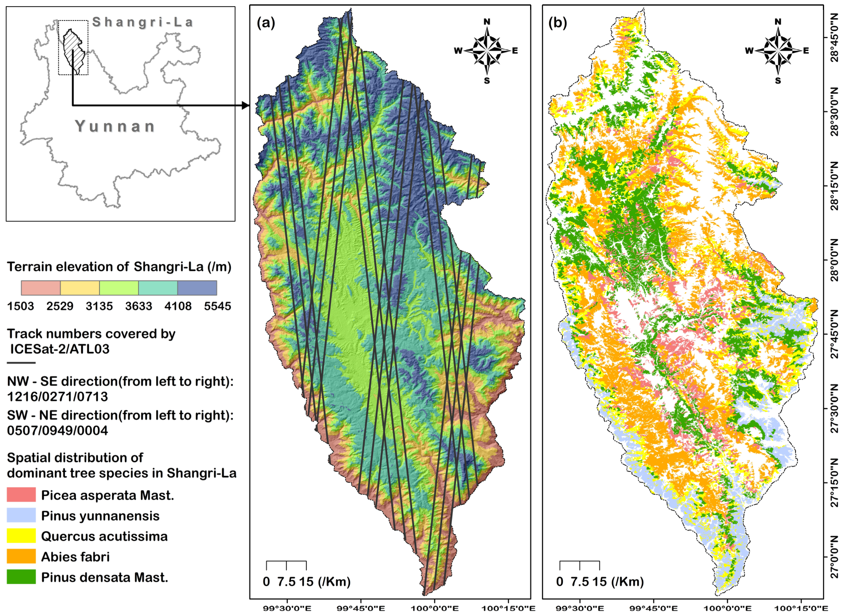
Shangri-La city, located in the range of 26°52′–28°52′N and 99°35′–100°35′E, is situated at the southeastern edge of the Qinghai-Tibet Plateau and the eastern part of the Three Parallel Rivers of Yunnan Protected Areas, which is a region where the Hengduan Mountains intersect. It is adjacent to Daocheng County and Muli Tibetan Autonomous County to the east and borders Derong County and Xiangcheng County to the north. It is connected to Deqin County, Weixi Lisu Autonomous County, and Yulong Naxi Autonomous County by a continuous stretch of mountains and rivers to the west and south. The general topographic trend of the city is high in the northwest and low in the southeast. Its highest point is Balagazong, at 5545 m above sea level, and its lowest point is Luojijihan, at 1503 m above sea level, with an altitude difference of 4042 m and an average altitude of 3459 m. The landform of Shangri-La can be divided into mountains, plateaus, basins, and valleys (Figure 1a), among which the mountain area is the largest landform type, with 10,541 km² above 2500 m, accounting for 93.5% of the city’s total area [28]. In addition, there are numerous well-stored primary forests and alpine meadow forest ecosystems in Shangri-La city, with a forest coverage rate of 76.00%, which can play an indispensable role in regulating the regional ecological environment and stabilizing regional biodiversity.

2.2. Data

2.2.1. ICESat-2/ATL03 Data

The ATLAS carried on the new generation of ICESat-2 adopts multi-beam micropulse photon counting Lidar technology, which is the first of its kind applied to the spaceborne satellite platform [29]. Compared with ICESat-1/GLAS, the system is characterized by high repetition frequency, density, and precision. In this study, the ICESat-2/ATLAS secondary product ATL03 is used for forest canopy height extraction and then to conduct the spatially continuous canopy height inversion using the spot-scale canopy height data as training samples combined with different inversion models. ATL03, which is global positioning photon data with parameters containing latitude, longitude, and elevation, is susceptible to interference from solar background noise, resulting in a large number of noise photons mixed in its signal photons. In addition, the retrieval of coverage data in the study area was performed through the OPENALTIMETRY [30] platform, and information such as coverage data time and orbit number was obtained and downloaded from the official platform of the NSIDC (https://nsidc.org/data/atl03/versions/5, accessed on 25 October 2022). Among them, Figure 1 and

Table 1. ICESat-2/ATL03 coverage data acquisition within the Shangri-La region.

Number	ICESat-2/ATL03 Info Date/RGT Number/Cycle Number/Segment Number	Strong Tracks
NW-SE_01	20181217/1216/01/02	gt1r/gt2r/gt3r
SW-NE_01	20190130/0507/02/06	gt1l/gt2l/gt3l
NW-SE_02	20181016/0271/01/02	gt1r/gt2r/gt3r
SW-NE_02	20181129/0949/01/06	gt1r/gt2r/gt3r
NW-SE_03	20190213/0713/02/02	gt1l/gt2l/gt3l
SW-NE_03	20181228/0004/02/06	gt1l/gt2l/gt3l

present the spatial location and parameter information of the coverage data.

2.2.2. Sentinel-2 Data

Sentinel-2 data were selected to extract explanatory variables for different inversion models in achieving spatially continuous inversion of forest canopy height in the Shangri-La region. Compared with Landsat-8 OLI image data, Sentinel-2 contains a more favorable red-edge correlation band for canopy height inversion [6]. Based on Sentinel-2 surface reflectance data for the period of 2018–2019 in the study area, cloud detection and repair of cloud-shadow areas were performed using the Google Earth Engine platform. Subsequently, the processed multi-temporal remote sensing images were stitched and fused. Finally, Sentinel-2 image data without cloud interference in the study area can be generated. In addition, the obtained image data should also be resampled to 30 m and corrected for terrain [31]. The above process can further moderate the effects of atmospheric conditions and topographic relief on the estimation of each explanatory variable and greatly improve the accuracy of the canopy height inversion model.

2.2.3. Other Auxiliary Data

The auxiliary data mainly include meteorological (average annual precipitation and temperature), topographic, and forest survey data. The annual average precipitation is obtained from the 1 km monthly average precipitation dataset of China from 1960 to 2020. The annual average temperature is obtained from the 1 km monthly average temperature dataset of China from 1901 to 2021 (National Center for Earth System Science Data: http://www.geodata.cn/, accessed on 25 October 2022). Both of these are resampled at 30 m. Topographic data are ASTER GDEM data (Geospatial Data Cloud: https://www.gscloud.cn/, accessed on 25 October 2022).

The forest survey data include forest plot data from the National Forest Resources Type II Survey and plot survey data collected by our research team in the study area. The plot survey data consist of high-precision forest height data acquired through years of accumulation (nearly 300 sample plots) using manual measurements, ground-based Lidar, and other methods. These data serve as validation samples for different canopy height inversion methods in this study. However, the geographical environment in the study area is extremely complex and, even with years of accumulation, the validation samples cannot cover all dominant tree species. Therefore, based on the requirements for representativeness and accuracy of the validation samples, a total of 50 measured sample points were obtained for forest height validation within the study area. Furthermore, the forest plot data from the National Forest Resources Type II Survey and plot survey provide information on the spatial distribution of all dominant tree species in the study area. Specifically, we selected Abies fabri, Pinus densata Mast., Quercus acutissima, Pinus yunnanensis, and Picea asperata Mast. as the main tree species for forest canopy height modeling. There are two reasons for this selection. Firstly, based on the forest plot data and literature [32], these five tree species represent the most widely distributed dominant tree species in the study area, accounting for 25%, 23%, 13%, 12%, and 10% of the total forest area, respectively. Secondly, according to the literature [33], the distribution of tree species in Shangri-La is mainly within the range of 2300–4700 m above sea level, with broad-leaved forests, mixed coniferous and broad-leaved forests, and coniferous forests distributed from low to high elevations. Meanwhile, the elevation distribution of the five dominant tree species is as follows: Abies fabri (3500–5000 m), Picea asperata Mast. (3000–4500 m), Pinus densata Mast. (2800–4000 m), Quercus acutissima (2000–4000 m), and Pinus yunnanensis (2000–3500 m). This reflects the different adaptability of dominant tree species to water and thermal conditions in the study area. In summary, based on the characteristics of dominant tree species in the study area as described in the literature [28] and the forest plot data, the selected dominant tree species fully reflect the horizontal and vertical zonality of the study area.

3. Research Methods

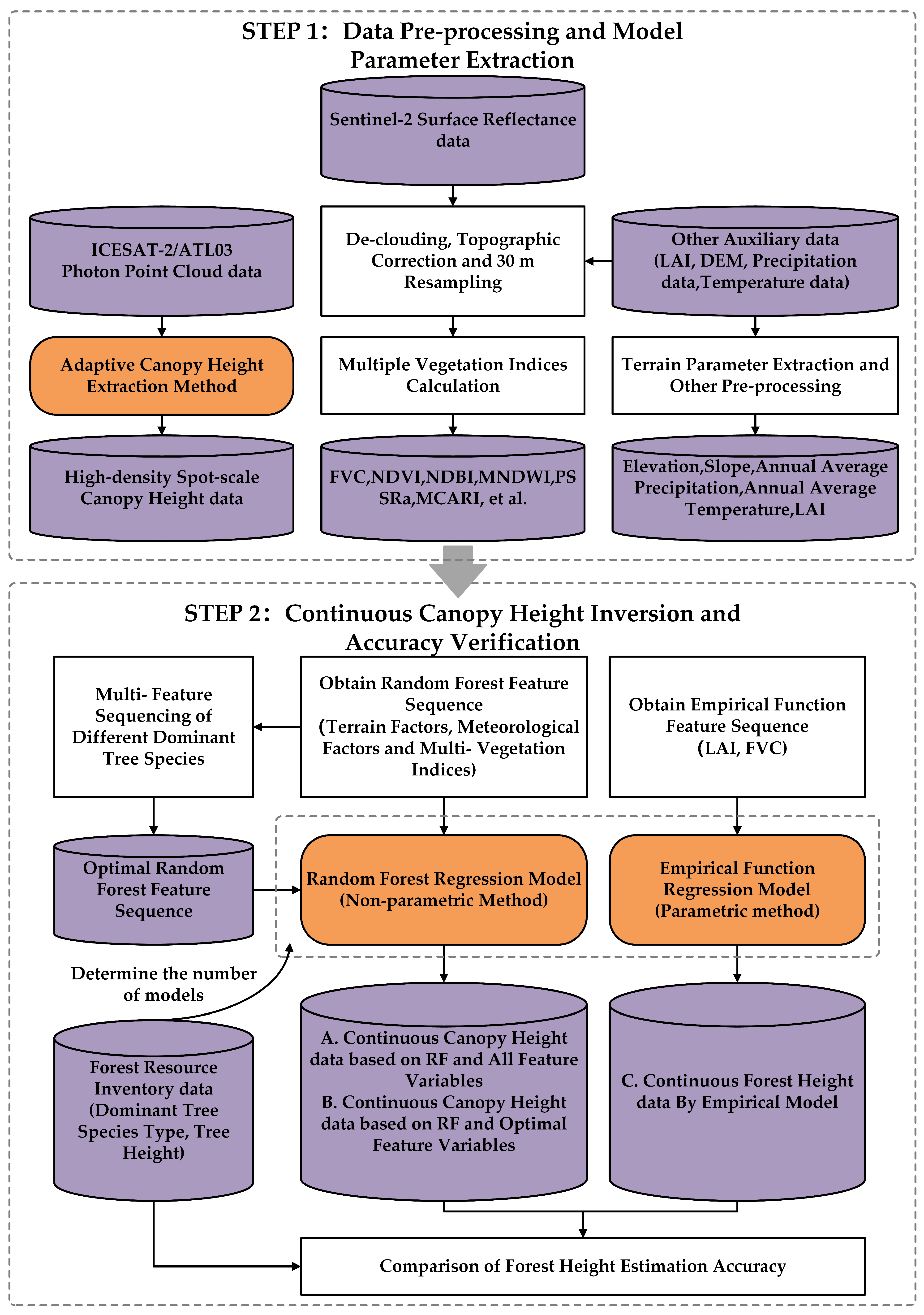
In this paper, different research methods were selected to conduct the spatially continuous forest canopy height inversion in the Shangri-La region, and the research idea is presented in Figure 2. The specific steps can be divided as follows: (1) Data preprocessing: to correct the atmosphere and topography of Sentinel-2 SR images and resampling of each auxiliary data. (2) Extraction of feature variables and training samples: (a) to extract the FVC and feature variables associated with random forest models based on pre-processed SR images; (b) to extract the canopy height data at the light spot scale based on ICESat-2 profile point clouds, which are regarded as training samples for different prediction models. (3) Construction of canopy height inversion models: (a) to construct the corresponding parametric models under different dominant tree species with FVC and LAI as explanatory variables and light spot scale canopy height data as training samples; (b) to construct the corresponding non-parametric model (i.e., random forest model) under different dominant tree species with all vegetation indices and geographic environment factors as explanatory variables and light spot scale canopy height as training samples; (c) to rank the importance of the explanatory variables involved in b’s nonparametric model, change the explanatory variables entered into the nonparametric model, and extract the combination of variables with the best accuracy; the process of constructing the nonparametric model under each dominant tree species is repeated with the best combination of variables as the new explanatory variables. (4) The inversion and accuracy verification and comparison of canopy height: to verify the accuracy of spatially continuous canopy height data extracted from different models in (3) and make comparison between different models.

3.1. Forest Canopy Height Extraction Algorithm of ICESat-2/ATL03

According to an algorithm for forest canopy height extraction proposed by Huang et al. [27], which is suitable for complex mountainous terrain, the specific steps are as follows: (1) Data preprocessing: to obtain two-dimensional profile point clouds at appropriate scales. (2) Point cloud denoising: to process point cloud by adopting the Threshold Segmentation based on Spatial Clustering and Bimodal Reconstruction (TS-SCABR) denoising algorithm. TS-SCABR is based on the characteristic that the spatial density of ICESat-2 signal photons is higher than that of noise photons. It performs local density counting on each photon based on an adaptive neighborhood radius (Equation (1)) and constructs a histogram. Considering the diversity of histogram distributions under different signal-to-noise ratios, it employs Gaussian decomposition to accurately extract the noise and signal peaks. Finally, a bimodal threshold segmentation is applied to separate the signal. (3) Point cloud classification: most of the noise can be removed from the profile point clouds through the denoising process of point clouds. In order to extract canopy height data, ground photons and canopy-top photons need to be further identified. In this process, methods such as iterative moving surface filtering and mutation detection are used to identify ground photons, and percentile statistics are used to identify canopy-top photons. (4) Canopy height extraction: to estimate the canopy height of current profile point cloud data through the difference between the elevation of the canopy-top photon and the ground photon whose position matches.

$$\left\{\begin{array}{c}R=\sqrt{\frac{P/N_{\mathrm{Total}}}{\pi }}\hfill \\ P=\mathrm{int}\left(2.96273\times SNR+2.24325\right)\hfill \end{array}\right.$$

(1)

In Formula (1), R stands for neighborhood search radius, $N_{Total}$ represents the total number of photons under processing segments, P is the neighborhood number, and SNR is the initial signal-to-noise ratio parameter estimated through the photon elevation frequency statistics.

3.2. Forest Canopy Height Inversion Model Based on the Empirical Function Regression

During the growth of vegetation, the leaf area of most vegetation has a simultaneous growth relationship with plant height [14]. Therefore, a conversion relationship between LAI and FVC ratio and plant height is proposed for different crop types and species. Dong et al. [16] fitted a more accurate relationship model between the LAI and FVC ratio and canopy height based on a logarithmic function for different forest types (including coniferous, broadleaf, and mixed forests) under this condition. The results of this study showed that R² of coniferous forest reached more than 0.733. Broad-leaved forest followed with an R² above 0.610. The R² of the mixed forest was 0.407. Therefore, based on the fact that canopy height data at the light spot scale estimated by ICESat-2/ATL03 are used as the training sample, the spatially continuous canopy height data under different dominant tree species in the Shangri-La region can be inverted by combining Equation (2). Among them, the results are estimated with LAI citing the estimation results of Yu et al. [34] (R² = 0.7903) and FVC relying on the dimidiate pixel model of Li [35] combined with Sentinel-2 SR data.

$${\mathrm{Height}}_{\mathrm{Canopy}}=f_{1\mathrm{n}}\left(LAI/FVC\right)$$

(2)

In Formula (2), $Heigh{t}_{Canopy}$ is the dependent variable, indicating the forest canopy height; $LAI/FVC$ is the independent variable, representing the ratio of LAI to FVC; and $f_{\ln }$ shows the logarithmic relationship between the independent variable and the dependent variable.

3.3. Forest Canopy Height Inversion Model Based on the Random Forest Regression

3.3.1. Random Forest Model Construction

Given the multicollinearity among feature parameters in optical image data, random forests are an ideal method to reduce the correlation between predicted values by introducing random perturbations into training samples and decision features, ultimately avoiding overfitting. Therefore, the random forest regression algorithm for model construction is proposed in this paper. The processing steps are listed as follows: (1) The random forest regression model is set with B regression trees, which is set to 500 in this paper. The current regression tree number is denoted as b, and the process in (2)–(3) is iteratively performed by setting b = 1, 2, 3, ..., B. (2) The discrete forest canopy height dataset with a sample size of N is resampled by bootstrap to obtain the bootstrap sample S_b of the regression tree of number b. The remaining samples are referred to as out-of-bag (OOB) data. (3) Based on the bootstrap sample S_b and input feature variable ${\mathsf{\Theta }}_{\mathrm{b}}$ and the built regression tree T_b, the predicted result is $T_b\left({\mathsf{\Theta }}_{\mathrm{b}}\right)$. (4) After B iterations, the final predicted result $f\left({\mathsf{\Theta }}_{\mathrm{b}}\right)$ is obtained (Equation (3)). An assessment of the importance of the input feature variables in process (3) is usually required to improve the efficiency of random forest regression modeling.

$$f\left({\mathsf{\Theta }}_b\right)=\frac{1}{B}{\displaystyle \sum }_{b=1}^B{T}_b\left({\mathsf{\Theta }}_b\right)$$

(3)

3.3.2. Selection and Ranking of Feature Variables

The surface reflectance of forest canopy depends on the optical properties of both the trees and the underlying soil [36,37]. Based on the basic characteristics of the spectral bands in the Sentinel-2 surface reflectance product, vegetation indices are calculated using only the green, red, vegetation red edge, near-infrared, water vapour, and shortwave infrared bands from the acquired Sentinel-2 dataset. The specific vegetation indices are selected based on the highly correlated characteristic variables for forest canopy height inversion, as described in [37,38,39,40]. In addition, to account for the effects of terrain, weather, and altitude on tree growth, factors such as elevation, slope, mean annual temperature, and mean annual precipitation are selected [41]. Furthermore, in order to avoid optical saturation issues caused by using multiple vegetation indices, a set of 20 parameters (Table 2) are selected as alternative characteristic variables.

For feature importance evaluation in random forest models, commonly used evaluation metrics include mean decrease in impurity (MDI) and mean decrease in accuracy (MDA). However, MDI can overestimate the importance of high-cardinality characteristic variables. This is because MDI evaluates feature importance by measuring the splitting contribution of each feature variable in each decision tree, which can result in high-cardinality feature variables being used for many splits, contributing significantly to the overall decrease in impurity [42]. In addition, MDI only considers the decrease in impurity of feature variables and not their correlations with other variables. In contrast, MDA is more comprehensive and fairer, as it evaluates feature variable importance by testing changes in the model’s predictive accuracy through the random permutation of each feature variable. MDA does not have the aforementioned limitations and can also detect overfitting in random forest models [43]. Therefore, we selected MDA calculated based on OOB data as the primary metric for ranking feature variables in our random forest model, with larger MDA values indicating greater feature variable importance.

According to the MDA feature importance evaluation, the importance ranking results of 20 feature variables under five dominant tree species (denoted as ${\mathsf{\Theta }}_{\mathrm{single}}$ for each species) can be obtained, and a comprehensive feature ranking (denoted as ${\mathsf{\Theta }}_{\mathrm{all}}$) can be obtained by superimposing the rankings of each dominant species. In this way, two sets of sorted feature sequences for each dominant tree species, ${\mathsf{\Theta }}_{\mathrm{single}}$ and ${\mathsf{\Theta }}_{\mathrm{all}}$, can be obtained. Subsequently, taking ${\mathsf{\Theta }}_{\mathrm{single}}$ as an example, feature combinations are selected in the order of ${\mathsf{\Theta }}_{\mathrm{single}}$ (starting from three and increasing by increments), and then a random forest regression model is input for prediction. R² and root mean square error (RMSE) are used as evaluation metrics to determine the optimal feature combination with the highest accuracy. The same process is applied to ${\mathsf{\Theta }}_{\mathrm{all}}$. Finally, the accuracy of the optimal feature combination corresponding to ${\mathsf{\Theta }}_{\mathrm{single}}$ and ${\mathsf{\Theta }}_{\mathrm{all}}$ is used for comparison.

Table 2. Information of feature variables in the random forest regression prediction model.

Feature Name	The Description of the Feature Variable	Reference
Slope	Topographic slope estimated based on elevation data.	-
Precipitation	Annual average precipitation data for the Shangri-La region.	-
Elevation	Shangri-la 30 m elevation data extracted by ASTER GDEM product mask.	-
Temperature	Annual average temperature data for the Shangri-La region.	-
Vapour	B9(Water Vapour)	-
SWIR1	B11(ShortWave InfraRed1)	-
VRE1	B5(Vegetation Red Edge1)	-
SWIR2	B12(ShortWave InfraRed2)	-
MTCI	$MTCI=\left(VRE2-VRE1\right)/\left(VRE1-R\right)$ VRE2-B6(Vegetation Red Edge2)/VRE1-B5(Vegetation Red Edge1)/R-B4(Red)	Dash et al. [44]
S2REP	$S2REP=705+35\times (\left(R+VRE3)/2-VRE1\right)/\left(VRE2-VRE1\right)$ R-B4(Red)/VRE3-B7(Vegetation Red Edge3)/VRE1-B5(Vegetation Red Edge1)/VRE2-B6(Vegetation Red Edge2)	Guyot et al. [45]
EVI	$EVI=2.5\times \left(NIR-R/NIR+6\times R-7.5\times B+1\right)$ NIR-B8(Near InfraRed)/R-B4(Red)	Liu et al. [46]
NDBI	$NDBI=\left(SWIR1-NIR\right)/\left(SWIR1+NIR\right)$ SWIR1-B11(ShortWave InfraRed1)/NIR-B8(Near InfraRed)	Zha et al. [47]
PSSRa	$PSSRa=VRE3/R$ VRE3-B7(Vegetation Red Edge3)/R-B4(Red)	Blackburn [48]
MNDWI	$MNDWI=\left(G-SWIR1\right)/\left(G+SWIR1\right)$ G-B3(Green)/SWIR1-B11(ShortWave InfraRed1)	Xu [49]
MCARI	$MCARI=\left(\left(VRE1-R\right)-0.2\times \left(VRE1-G\right)\right)\times \left(VRE1/R\right)$ VRE1-B5(Vegetation Red Edge1)/R-B4(Red)/G-B3(Green)	Daughtry et al. [50]
IRECI	$IRECI=\left(VRE3-R\right)/\left(VRE1/VRE2\right)$ VRE1-B5(Vegetation Red Edge1)/VRE2-B6(Vegetation Red Edge2)/VRE3-B7(Vegetation Red Edge3)/R-B4(Red)	Clevers et al. [51]
FDI	$FDI=NIR-\left(G+R\right)$ NIR-B8(Near InfraRed)/G-B3(Green)/R-B4(Red)	Bunting et al. [52]
NDWI	$NDWI=\left(G-NIR\right)/\left(G+NIR\right)$ G-B3(Green)/NIR-B8(Near InfraRed)	McFeeters [53]
NDVI	$NDVI=\left(NIR-R\right)/\left(NIR+R\right)$ NIR-B8(Near InfraRed)/R-B4(Red)	Rouse et al. [54]
RVI	$RVI=NIR/R$ NIR-B8(Near InfraRed)/R-B4(Red)	Major et al. [55]

Table 2. Information of feature variables in the random forest regression prediction model.

Feature Name	The Description of the Feature Variable	Reference
Slope	Topographic slope estimated based on elevation data.	-
Precipitation	Annual average precipitation data for the Shangri-La region.	-
Elevation	Shangri-la 30 m elevation data extracted by ASTER GDEM product mask.	-
Temperature	Annual average temperature data for the Shangri-La region.	-
Vapour	B9(Water Vapour)	-
SWIR1	B11(ShortWave InfraRed1)	-
VRE1	B5(Vegetation Red Edge1)	-
SWIR2	B12(ShortWave InfraRed2)	-
MTCI	$MTCI=\left(VRE2-VRE1\right)/\left(VRE1-R\right)$ VRE2-B6(Vegetation Red Edge2)/VRE1-B5(Vegetation Red Edge1)/R-B4(Red)	Dash et al. [44]
S2REP	$S2REP=705+35\times (\left(R+VRE3)/2-VRE1\right)/\left(VRE2-VRE1\right)$ R-B4(Red)/VRE3-B7(Vegetation Red Edge3)/VRE1-B5(Vegetation Red Edge1)/VRE2-B6(Vegetation Red Edge2)	Guyot et al. [45]
EVI	$EVI=2.5\times \left(NIR-R/NIR+6\times R-7.5\times B+1\right)$ NIR-B8(Near InfraRed)/R-B4(Red)	Liu et al. [46]
NDBI	$NDBI=\left(SWIR1-NIR\right)/\left(SWIR1+NIR\right)$ SWIR1-B11(ShortWave InfraRed1)/NIR-B8(Near InfraRed)	Zha et al. [47]
PSSRa	$PSSRa=VRE3/R$ VRE3-B7(Vegetation Red Edge3)/R-B4(Red)	Blackburn [48]
MNDWI	$MNDWI=\left(G-SWIR1\right)/\left(G+SWIR1\right)$ G-B3(Green)/SWIR1-B11(ShortWave InfraRed1)	Xu [49]
MCARI	$MCARI=\left(\left(VRE1-R\right)-0.2\times \left(VRE1-G\right)\right)\times \left(VRE1/R\right)$ VRE1-B5(Vegetation Red Edge1)/R-B4(Red)/G-B3(Green)	Daughtry et al. [50]
IRECI	$IRECI=\left(VRE3-R\right)/\left(VRE1/VRE2\right)$ VRE1-B5(Vegetation Red Edge1)/VRE2-B6(Vegetation Red Edge2)/VRE3-B7(Vegetation Red Edge3)/R-B4(Red)	Clevers et al. [51]
FDI	$FDI=NIR-\left(G+R\right)$ NIR-B8(Near InfraRed)/G-B3(Green)/R-B4(Red)	Bunting et al. [52]
NDWI	$NDWI=\left(G-NIR\right)/\left(G+NIR\right)$ G-B3(Green)/NIR-B8(Near InfraRed)	McFeeters [53]
NDVI	$NDVI=\left(NIR-R\right)/\left(NIR+R\right)$ NIR-B8(Near InfraRed)/R-B4(Red)	Rouse et al. [54]
RVI	$RVI=NIR/R$ NIR-B8(Near InfraRed)/R-B4(Red)	Major et al. [55]

4. Results and Analysis

4.1. Inversion Results of the Forest Canopy Height Based on the Empirical Function Regression

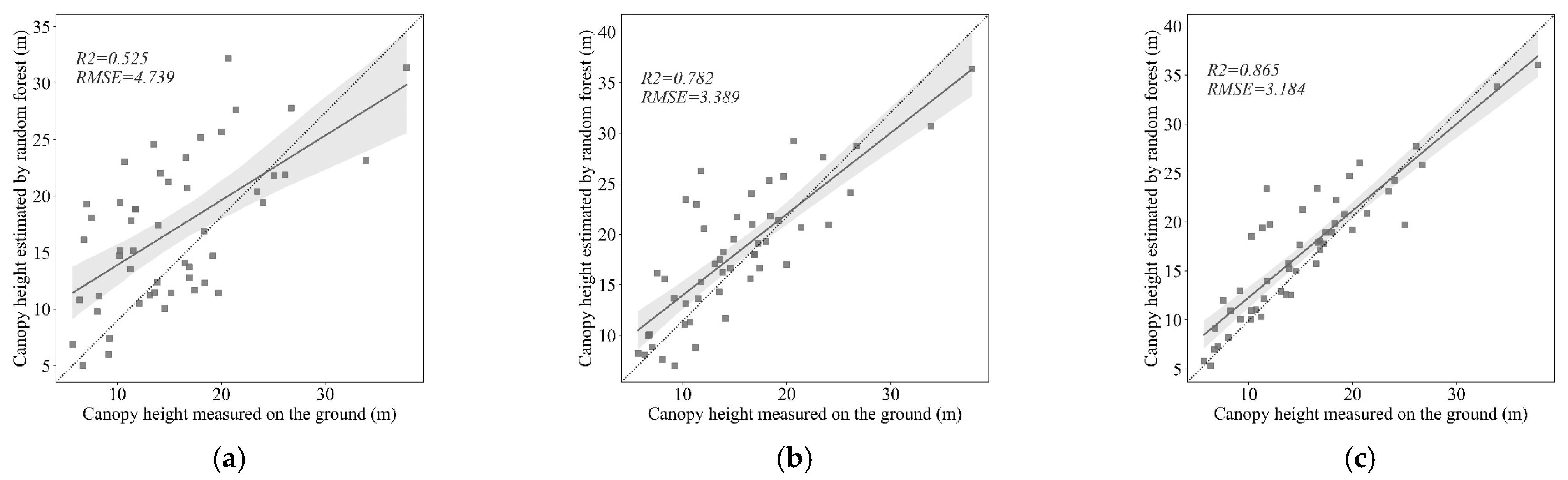
According to the ICESat-2/ATL03 forest canopy height extraction algorithm described in Section 3.1, sufficient forest canopy height data for the Shangri-La area were extracted from the collected photon point cloud data in Table 1. A total of 220,957 data points were processed as the training dataset. When developing the canopy height inversion model for different dominant tree species by fitting the functional relationship in Equation (2), 200 data points were uniformly sampled from each region of the dominant tree species. These data points were then divided at a ratio of 7:3 between training and testing samples. Dong [16] also used the same function relationship to fit canopy height models for different forest types (coniferous forest, broad-leaved forest, and mixed forest) in Jiangxi, with an R² mean value of 0.583. In comparison, this study has a slightly better fitting effect, with an R² mean value of 0.595. Regression t-tests were conducted on the parametric models for different dominant tree species, which show all reached extremely significant levels (p < 0.05). The higher accuracy in this study is attributed to the selection of high-precision training samples and adjustments to specific parametric models. It can be seen that the canopy height extraction algorithm proposed by Huang et al. [27] has high research value under complex terrain conditions, but relatively low applicability of the parametric model in different study areas. In addition, among the different dominant tree species, relatively poor fitting effects were shown in Quercus acutissima and Pinus yunnanensis, with R² values of 0.545 and 0.526, respectively, while relatively good fitting effects were shown in Pinus densata Mast., Picea asperata Mast., and Abies fabri, with R² values of 0.665, 0.623, and 0.616, respectively. Among all of the dominant tree species, the former ones, mainly distributed in the high altitude area of Shangri-La, with narrow ecological range and large habitat restriction, as well as poor heterogeneous tree composition, are typical coniferous forests. The latter ones, usually distributed in the middle and low altitudes in the south of Shangri-La, with a wide ecological range and less habitat restriction, are often mixed with other tree species [32]. According to the study in the literature [16], Equation (2) is more adaptable to coniferous forests and less adaptable to mixed forests, which explains the differences in fitting performance among different dominant tree species. Finally, based on the different dominant tree species canopy height models in

Table 3. Parametric model fitting under different dominant tree species.

Dominant Tree Species	Number of Training and Testing Samples	Model Information			R2	Regression t-Test (p-Value)
		Equation	α	β
Abies fabri	200	$\left\{\begin{array}{c}\mathrm{Y}=\alpha \ast \mathrm{Ln}\left(-\mathsf{\beta }\ast \mathrm{Ln}\left(\mathrm{X}\right)\right)\\ \mathrm{Y}: \mathrm{Canopy} \mathrm{Height}\\ \mathrm{X}:\mathrm{LAI}/\mathrm{FVC}\end{array}\right.$	−21.16577	−0.38467	0.616	5.337 × 10−9
Pinus densata Mast.	200		−36.42064	−0.57092	0.665	3.764 × 10−9
Quercus acutissima	200		−18.11949	−0.27552	0.545	1.471 × 10−6
Pinus yunnanensis	200		−10.17889	−0.32941	0.526	1.401 × 10−9
Picea asperata Mast.	200		−19.65823	−0.51156	0.623	3.396 × 10−6

, this study achieved spatially continuous forest canopy height inversion in the Shangri-La area (Figure 4a), and the accuracy was validated with 50 ground-measured data points, with an R² of 0.525 and an RMSE of 4.739 m (Figure 5a).

4.2. Inversion Results of the Forest Canopy Height Based on the Random Forest Regression

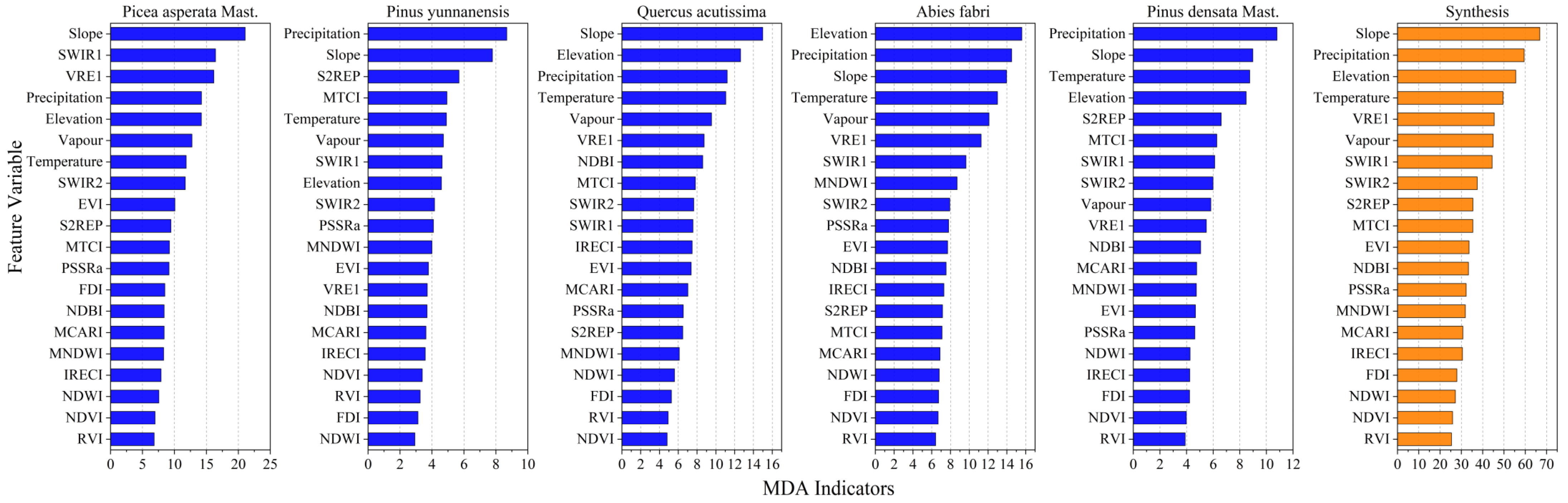
Because of the insensitivity of the random forest regression model to collinearity problems, all feature variables can be included in the model. However, to improve the modeling efficiency of the random forest model, feature importance is evaluated by adopting the random forest regression model. After multiple research tests, the empirical function model was found to possess an explicit expression that allows it to approach stability with limited sample sizes, in contrast to the random forest model, which requires extensive sample data for training [56,57]. Therefore, for different dominant tree species, even with a foundation of 200 samples used to train the empirical function model, additional samples are still required to train the random forest model until the estimated accuracy of the corresponding testing samples approaches stability. The criterion for dividing the training and testing samples remains at a 7:3 ratio. Figure 3 shows the importance evaluation results of 20 selected feature variables for different dominant tree species regions based on random forest regression and MDA indicators. The data show that the canopy height inversion of the Picea asperata Mast. is highly correlated with Slope, SWIR1, and VRE1; the canopy height inversion of the Pinus yunnanensis is highly correlated with Precipitation, Slope, and S2REP; the canopy height inversion of the Quercus acutissima is highly correlated with Slope, Elevation, and Precipitation; the canopy height inversion of the Abies fabri is highly correlated with Precipitation, Elevation, and Slope; and the canopy height inversion of the Pinus densata Mast. is highly correlated with Precipitation, Temperature, and Slope. Meanwhile, the feature importance ranking of five dominant tree species was comprehensively synthesized by summing them up, and it was found that Precipitation, Elevation, and Slope are highly correlated with canopy height inversion in the Shangri-La region. The evaluation results mentioned above are consistent with the results in the literature [1], indicating that terrain and meteorological conditions can present local variation characteristics of forest canopy height. Therefore, it can be concluded that meteorological and topographic factors play a dominant role in the canopy height inversion of different dominant tree species in the Shangri-La region.

In Figure 3 above, the feature ranking results of ${\mathsf{\Theta }}_{\mathrm{single}}$ and ${\mathsf{\Theta }}_{\mathrm{all}}$ for different dominant tree species can be obtained as input parameters for the random forest regression model, among which the number of input parameters is adjusted in descending order of importance (starting from three). In this way, the input parameters with the highest prediction accuracy under the two feature sequences can then be obtained (i.e., rows 1–2 of

Table 4. Inversion accuracy of canopy height under different combinations of feature variables.

Dominant Tree Species	Feature Selection for Random Forest Regression Models	RMSE (m)	R2
Picea asperata Mast.	Slope/SWIR1/VRE1/Precipitation/Elevation/Vapour(S2 B9)/Temperature	4.086	0.736
	Slope/Precipitation/Elevation/Temperature/Vapour(S2 B9)	3.994	0.756
	All feature vectors	4.254	0.712
Pinus densata Mast.	Precipitation/Slope/Temperature/Elevation/S2REP/MTCI/SWIR1/SWIR2/Vapour(S2 B9)	3.774	0.725
	Slope/Precipitation/Elevation/Temperature/Vapour(S2 B9)/SWIR1	3.210	0.762
	All feature vectors	3.893	0.712
Abies fabri	Elevation/Precipitation/Slope/Temperature/Vapour(S2 B9)/VRE1/SWIR1/MNDWI/SWIR2	3.796	0.760
	Slope/Precipitation/Elevation/Temperature/Vapour(S2 B9)/SWIR1/VRE1/SWIR2/MTCI	3.820	0.757
	All feature vectors	4.739	0.748
Pinus yunnanensis	Precipitation/Slope/S2REP/MTCI/Temperature/Vapour(S2 B9)/SWIR1/Elevation/SWIR2/PSSRa/MNDWI	3.997	0.681
	Slope/Precipitation/Elevation/Temperature/Vapour(S2 B9)/SWIR1	3.868	0.704
	All feature vectors	4.084	0.668
Quercus acutissima	Slope/Elevation/Precipitation/Temperature/Vapour(S2 B9)	5.103	0.720
	Slope/Precipitation/Elevation/Temperature/Vapour(S2 B9)	5.108	0.713
	All feature vectors	5.365	0.677

Note: Table 4 above shows the random forest prediction accuracy of different dominant tree species under different selected feature variables. Among the three groups of feature variables listed within each dominant tree species, the first set is the feature combined with the highest prediction accuracy corresponding to the top 20 feature variable importance rankings of the dominant tree species; the second set is the feature combination with the best prediction accuracy corresponding to the top 20 feature variable importance rankings of the five dominant tree species combined; and the third set includes all feature variables.

for each dominant tree species). Furthermore, the optimal results of the two feature sequences are compared to obtain the group with higher prediction accuracy as the final optimal variable for the dominant tree species (i.e., row 2 of Table 4). Meanwhile, compared with the accuracy of the random forest regression model for different dominant tree species in Table 4, the accuracy of Quercus acutissima and Pinus yunnanensis is lower. Liu et al. [58] proposed that there exist two problems when using random forest regression for continuous inversion of canopy height: (1) the training samples are covered by the prediction results of random forest regression, which will result in a decrease in the accuracy of canopy height data; (2) the saturation effect of optical images in forest parameter estimation remains. All of these explain the disadvantage of Quercus acutissima and Pinus yunnanensis in the above problems. In addition, the random forest regression model based on the final optimal variable for different dominant tree species has better accuracy than the one based on all feature variables, indicating that there is an error accumulation in random forest regression with the application of multiple feature variables, instead of the fact that the accuracy of random forest regression does not increase with more feature variables.

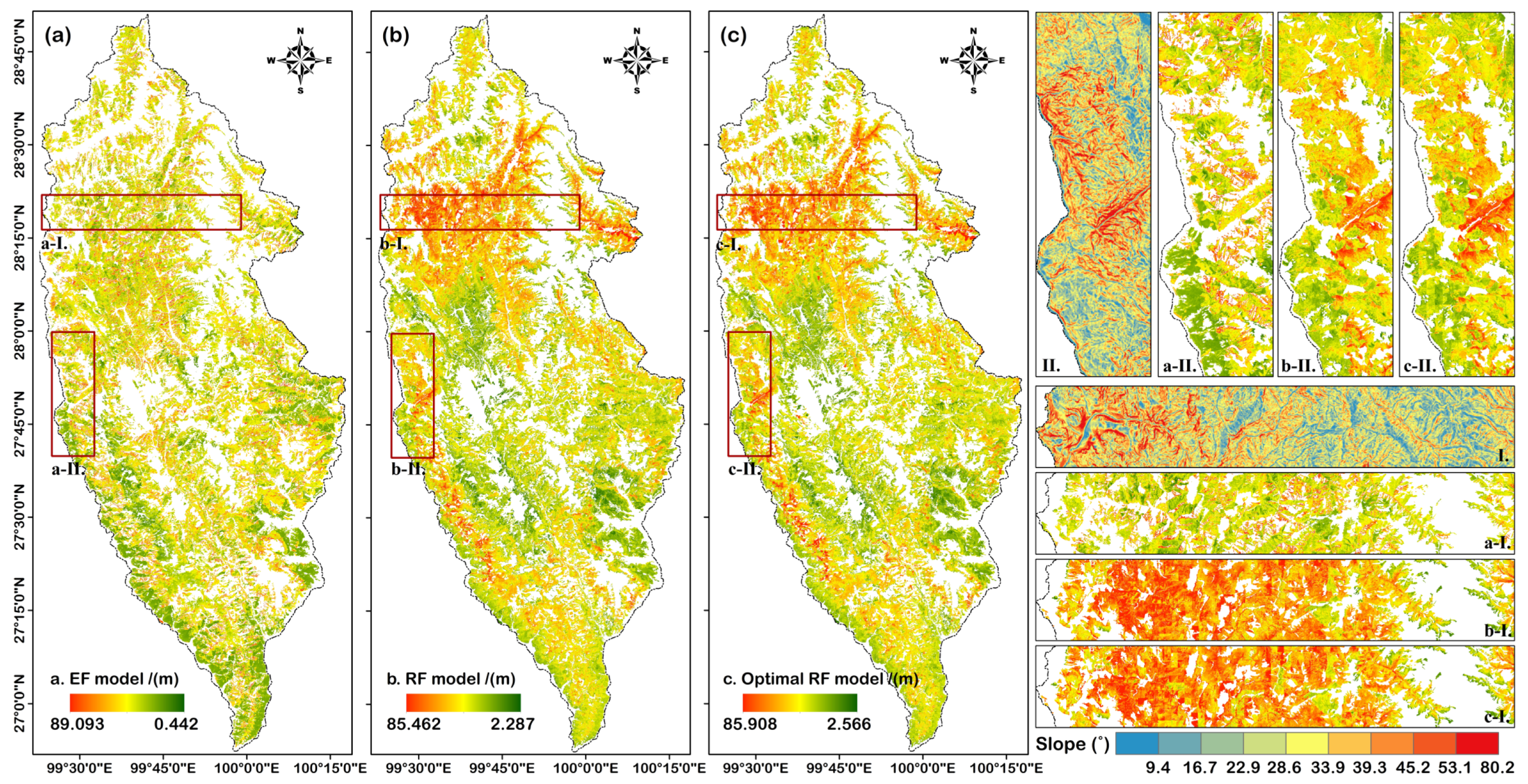
Continuous canopy height data for the Shangri-La area were obtained based on the optimal feature selection for different dominant tree species and all feature variables. At the same time, 50 ground-measured canopy height data points were used for accuracy validation. Figure 4b shows the random forest regression prediction results based on all feature variables, with R² = 0.782 and RMSE = 3.389 m (Figure 5b); Figure 4c shows the random forest regression prediction results based on the optimal feature selection, with R² = 0.865 and RMSE = 3.184 m (Figure 5c). Therefore, the inversion results of the empirical function indicate that the random forest regression model with optimal feature selection can obtain the best accuracy for canopy height data. What is more, based on the comparison of the estimation results of Figure 4a–c, it can be seen that the forest canopy height results have a larger deviation (a-I and c-I, a-II and c-II) under complex terrain conditions (such as scenarios I and II). According to the intelligent classification of dominant tree species in Shangri-La in the literature [32], topographic and meteorological factors are the key factors that distinguish Pinus densata Mast. and Abies fabri from other tree species, and the average height of Pinus densata Mast. and Abies fabri is higher than that of other tree species according to the forest resources survey data. Consequently, it can be seen that Shangri-La’s overripe forest mostly belongs to Pinus densata Mast. and Abies fabri. However, there are estimation errors in the parameter model in literature [16], although by using the ICESat-2 footprint-scale canopy height as samples for training. On the one hand, the representativeness of training samples in different age groups has a greater impact on this model than on the random forest model. On the other hand, this model lacks consideration of geographical and environmental factors and clear limitations under complex terrain conditions.

5. Conclusions

In this paper, the discrete forest canopy height data estimated from ICESat-2 profile point clouds are adopted as training samples to invert the continuous forest canopy height data in the Shangri-La area with parameter models and random forest regression models. Further, the applicability of different canopy height inversion algorithms under complex mountainous conditions is evaluated, and high-precision and spatially continuous forest canopy height data in the Shangri-La area are obtained at the same time. The research conclusions of this paper are as follows:

• The empirical function model cited in this paper has poor applicability under different terrain conditions, especially in complex terrain conditions where the fitting effect is relatively poor. In addition, during the fitting process of the empirical function model for each dominant tree species, the fitting effect is poor in Quercus acutissima and Pinus yunnanensis. At the meantime, because the ecological range of Quercus acutissima and Pinus yunnanensis in Shangri-La is wide, and the habitat limitation is small, it can be judged that their forest types are mostly mixed forests, which is similar to the results in previous research [16].
• It was found that the topographic and meteorological factors played a dominant role in canopy height inversion in evaluating the importance of explanatory variables in the random forest regression model.
• There are usually two problems when using random forest regression for canopy height inversion: the explanatory variables calculated from optical images can be subject to saturation, and there may be errors between the predicted results and the canopy height samples estimated by ICESat-2, especially in Quercus acutissima and Pinus yunnanensis. Furthermore, there may be an accumulation of errors in the random forest regression by applying multiple feature variables.
• Combining empirical function regression and random forest regression models, the highest precision canopy height data in Shangri-La can be obtained in the random forest regression model with the optimal feature variables, with an R² of 0.865 and an RMSE of only 3.184 m. In addition, the poor inversion effect of the parametric model is primarily due to the lack of consideration of topographical and meteorological factors, which is unsuitable for canopy height inversion under complex terrain conditions.

References

- Yang, T.; Wang, C.; Li, G.; Luo, S.; Xi, X.; Gao, S.; Zeng, H. Forest Canopy Height Mapping over China Using GLAS and MODIS Data. Sci. China Earth Sci. 2015, 58, 96–105. [Google Scholar] [CrossRef]
- Wu, L.; Zhu, Q. Impacts of the Carbon Emission Trading System on China’s Carbon Emission Peak: A New Data-Driven Approach. Nat. Hazards 2021, 107, 2487–2515. [Google Scholar] [CrossRef]
- Zhang, Y.; Li, S.; Luo, T.; Gao, J. The Effect of Emission Trading Policy on Carbon Emission Reduction: Evidence from an Integrated Study of Pilot Regions in China. J. Clean. Prod. 2020, 265, 121843. [Google Scholar] [CrossRef]
- Simard, M.; Pinto, N.; Fisher, J.B.; Baccini, A. Mapping Forest Canopy Height Globally with Spaceborne Lidar. J. Geophys. Res. 2011, 116, G04021. [Google Scholar] [CrossRef]
- Balzter, H.; Rowland, C.; Saich, P. Forest Canopy Height and Carbon Estimation at Monks Wood National Nature Reserve, UK, Using Dual-Wavelength SAR Interferometry. Remote Sens. Environ. 2007, 108, 224–239. [Google Scholar] [CrossRef]
- Li, W.; Niu, Z.; Shang, R.; Qin, Y.; Wang, L.; Chen, H. High-Resolution Mapping of Forest Canopy Height Using Machine Learning by Coupling ICESat-2 LiDAR with Sentinel-1, Sentinel-2 and Landsat-8 Data. Int. J. Appl. Earth Obs. 2020, 92, 102163. [Google Scholar] [CrossRef]
- Pierce, A.D.; Farris, C.A.; Taylor, A.H. Use of Random Forests for Modeling and Mapping Forest Canopy Fuels for Fire Behavior Analysis in Lassen Volcanic National Park, California, USA. For. Ecol. Manag. 2012, 279, 77–89. [Google Scholar] [CrossRef]
- Tang, H.; Brolly, M.; Zhao, F.; Strahler, A.H.; Schaaf, C.L.; Ganguly, S.; Zhang, G.; Dubayah, R. Deriving and Validating Leaf Area Index (LAI) at Multiple Spatial Scales through Lidar Remote Sensing: A Case Study in Sierra National Forest, CA. Remote Sens. Environ. 2014, 143, 131–141. [Google Scholar] [CrossRef]
- Gupta, R.; Sharma, L.K. Mixed Tropical Forests Canopy Height Mapping from Spaceborne LiDAR GEDI and Multisensor Imagery Using Machine Learning Models. Remote Sens. Appl. Soc. Environ. 2022, 27, 100817. [Google Scholar] [CrossRef]
- Sothe, C.; Gonsamo, A.; Lourenço, R.B.; Kurz, W.A.; Snider, J. Spatially Continuous Mapping of Forest Canopy Height in Canada by Combining GEDI and ICESat-2 with PALSAR and Sentinel. Remote Sens. 2022, 14, 5158. [Google Scholar] [CrossRef]
- Selkowitz, D.J.; Green, G.; Peterson, B.; Wylie, B. A Multi-Sensor Lidar, Multi-Spectral and Multi-Angular Approach for Mapping Canopy Height in Boreal Forest Regions. Remote Sens. Environ. 2012, 121, 458–471. [Google Scholar] [CrossRef]
- Yue, C.Y.; Zheng, Y.C.; Xing, Y.Q.; Pang, Y.; Li, S.M.; Cai, L.T.; He, H.Y. Technical and application development study of space-borne LiDAR in forestry remote sensing. Infrared Laser Eng. 2020, 49, 20200235. [Google Scholar]
- Liao, K.T. Estimation of Forest Aboveground Biomass in Jiangxi Province Using GLAS and Landsat Data. Master’s Thesis, Jiangxi Normal University, Nanchang, China, 2015. [Google Scholar]
- Zhang, R.H. Model on Remote Sensing and the Basic Experiments; Sciences Press: Beijing, China, 1996; pp. 20–60. [Google Scholar]
- Ghosh, S.M.; Behera, M.D.; Paramanik, S. Canopy Height Estimation Using Sentinel Series Images through Machine Learning Models in a Mangrove Forest. Remote Sens. 2020, 12, 1519. [Google Scholar] [CrossRef]
- Dong, L.X.; Li, G.C.; Tang, S.H. Inversion of forest canopy height in south of China by integrating GLAS and MERSI: The case of Jiangxi province in China. J. Remote Sens. 2011, 15, 1301–1314. [Google Scholar]
- Ni, X.; Zhou, Y.; Cao, C.; Wang, X.; Shi, Y.; Park, T.; Choi, S.; Myneni, R.B. Mapping Forest Canopy Height over Continental China Using Multi-Source Remote Sensing Data. Remote Sens. 2015, 7, 8436–8452. [Google Scholar] [CrossRef]
- Ni, X.; Park, T.; Choi, S.; Shi, Y.; Cao, C.; Wang, X.; Lefsky, M.A.; Simard, M.; Myneni, R.B. Allometric Scaling and Resource Limitations Model of Tree Heights: Part 3. Model Optimization and Testing over Continental China. Remote Sens. 2014, 6, 3533–3553. [Google Scholar] [CrossRef]
- Zhu, X.X. Based on ICESat-2 and GEDI Data, Research on Forest Height Retrieval with 30 m Resolution in China. Ph.D. Thesis, The Institute of Remote Sensing and Digital Earth (RADI), Chinese Academy of Sciences, Beijing, China, 2021. [Google Scholar]
- Luo, S.; Wang, C.; Xi, X.; Nie, S.; Fan, X.; Chen, H.; Ma, D.; Liu, J.; Zou, J.; Lin, Y.; et al. Estimating Forest Aboveground Biomass Using Small-Footprint Full-Waveform Airborne LiDAR Data. Int. J. Appl. Earth Obs. 2019, 83, 101922. [Google Scholar] [CrossRef]
- Lang, N.; Kalischek, N.; Armston, J.; Schindler, K.; Dubayah, R.; Wegner, J.D. Global Canopy Height Regression and Uncertainty Estimation from GEDI LIDAR Waveforms with Deep Ensembles. Remote Sens. Environ. 2022, 268, 112760. [Google Scholar] [CrossRef]
- Fayad, I.; Baghdadi, N.; Alcarde Alvares, C.; Stape, J.L.; Bailly, J.S.; Scolforo, H.F.; Cegatta, I.R.; Zribi, M.; Le Maire, G. Terrain Slope Effect on Forest Height and Wood Volume Estimation from GEDI Data. Remote Sens. 2021, 13, 2136. [Google Scholar] [CrossRef]
- Markus, T.; Neumann, T.; Martino, A.; Abdalati, W.; Brunt, K.; Csatho, B.; Farrell, S.; Fricker, H.; Gardner, A.; Harding, D.; et al. The Ice, Cloud, and Land Elevation Satellite-2 (ICESat-2): Science Requirements, Concept, and Implementation. Remote Sens. Environ. 2017, 190, 260–273. [Google Scholar] [CrossRef]
- Liu, A.; Cheng, X.; Chen, Z. Performance Evaluation of GEDI and ICESat-2 Laser Altimeter Data for Terrain and Canopy Height Retrievals. Remote Sens. Environ. 2021, 264, 112571. [Google Scholar] [CrossRef]
- Tian, X.; Shan, J. Comprehensive Evaluation of the ICESat-2 ATL08 Terrain Product. IEEE Trans. Geosci. Remote Sens. 2021, 59, 8195–8209. [Google Scholar] [CrossRef]
- Malambo, L.; Popescu, S.C. Assessing the Agreement of ICESat-2 Terrain and Canopy Height with Airborne Lidar over US Ecozones. Remote Sens. Environ. 2021, 266, 112711. [Google Scholar] [CrossRef]
- Huang, X.; Cheng, F.; Wang, J.; Duan, P.; Wang, J. Forest Canopy Height Extraction Method Based on ICESat-2/ATLAS Data. IEEE Trans. Geosci. Remote Sens. 2023, 61, 5700814. [Google Scholar] [CrossRef]
- Wang, J.L.; Cheng, F.; Wang, C.; Chen, L.J.; Wang, X.H. Primary Discussion on the Potential of Forest Volume Estimating Using ICESat/GLAS Data in Complex Terrain Area—A Case Study of Shangri-la Yunnan Province. Remote Sens. Technol. Appl. 2012, 27, 45–50. [Google Scholar]
- Zhu, X.X.; Wang, C.; Xi, X.H.; Nie, S.; Yang, X.B.; Li, D. Research progress of ICESat-2/ATLAS data processing and appli-cations. Infrared Laser Eng. 2020, 47, 76–85. [Google Scholar]
- Khalsa, S.J.S.; Borsa, A.; Nandigam, V.; Phan, M.; Lin, K.; Crosby, C.; Fricker, H.; Baru, C.; Lopez, L. OpenAltimetry-Rapid Analysis and Visualization of Spaceborne Altimeter Data. Earth Sci. Inform. 2022, 15, 1471–1480. [Google Scholar] [CrossRef]
- Soenen, S.A.; Peddle, D.R.; Coburn, C.A. SCS+C: A Modified Sun-Canopy-Sensor Topographic Correction in Forested Terrain. IEEE Trans. Geosci. Remote Sens. 2005, 43, 2148–2159. [Google Scholar] [CrossRef]
- Fang, P.F.; Wang, L.G.; Xu, W.H.; Ou, G.L.; Dai, Q.L.; Li, R.N. Decision Fusion Classification of Forest Dominant Tree Species in Shangri-La Area of Yunnan Province. Remote Sens. Technol. Appl. 2022, 37, 638–650. [Google Scholar]
- Ma, R.B.; Cheng, F.; Yi, B.J.; Fu, L.; Jiang, L.F. Analysis of vertical differentiation of land use in Shangri-La. J. Yunnan Norm. Univ. Nat. Sci. 2011, 31, 70–75. [Google Scholar]
- Yu, Y.; Wang, J.; Liu, G.; Cheng, F. Forest Leaf Area Index Inversion Based on Landsat OLI Data in the Shangri-La City. J. Indian Soc. Remote Sens. 2019, 47, 967–976. [Google Scholar] [CrossRef]
- Li, M.M. The Method of Vegetation Fraction Estimation by Remote Sensing. Master’s Thesis, The Institute of Remote Sensing and Digital Earth (RADI), Chinese Academy of Sciences, Beijing, China, 2003. [Google Scholar]
- Myneni, R.B.; Hall, F.G.; Sellers, P.J.; Marshak, A.L. The Interpretation of Spectral Vegetation Indexes. IEEE Trans. Geosci. Remote Sens. 1995, 33, 481–486. [Google Scholar] [CrossRef]
- Wang, H.; Seaborn, T.; Wang, Z.; Caudill, C.C.; Link, T.E. Modeling Tree Canopy Height Using Machine Learning over Mixed Vegetation Landscapes. Int. J. Appl. Earth Obs. 2021, 101, 102353. [Google Scholar] [CrossRef]
- Torres de Almeida, C.; Gerente, J.; Rodrigo dos Prazeres Campos, J.; Caruso Gomes Junior, F.; Providelo, L.A.; Marchiori, G.; Chen, X. Canopy Height Mapping by Sentinel 1 and 2 Satellite Images, Airborne LiDAR Data, and Machine Learning. Remote Sens. 2022, 14, 4112. [Google Scholar] [CrossRef]
- Deng, Y.; Pan, J.; Wang, J.; Liu, Q.; Zhang, J. Mapping of Forest Biomass in Shangri-La City Based on LiDAR Technology and Other Remote Sensing Data. Remote Sens. 2022, 14, 5816. [Google Scholar] [CrossRef]
- Nandy, S.; Srinet, R.; Padalia, H. Mapping Forest Height and Aboveground Biomass by Integrating ICESat-2, Sentinel-1 and Sentinel-2 Data Using Random Forest Algorithm in Northwest Himalayan Foothills of India. Geophys. Res. Lett. 2021, 48, e2021GL093799. [Google Scholar] [CrossRef]
- Moudrý, V.; Gdulová, K.; Gábor, L.; Šárovcová, E.; Barták, V.; Leroy, F.; Špatenková, O.; Rocchini, D.; Prošek, J. Effects of Environmental Conditions on ICESat-2 Terrain and Canopy Heights Retrievals in Central European Mountains. Remote Sens. Environ. 2022, 279, 113112. [Google Scholar] [CrossRef]
- Jindal, R.; Leekha, M.; Manuja, M.; Goswami, M. What Makes a Better Companion? Towards Social & Engaging Peer Learning. In Proceedings of the 24th European Conference on Artificial Intelligence (ECAI), Santiago de Compostela, Spain, 29 August–8 September 2020; pp. 482–489. [Google Scholar]
- Hur, J.-H.; Ihm, S.-Y.; Park, Y.-H. A Variable Impacts Measurement in Random Forest for Mobile Cloud Computing. Wirel. Commun. Mob. Comput. 2017, 2017, e6817627. [Google Scholar] [CrossRef]
- Dash, J.; Curran, P.J. Evaluation of the MERIS Terrestrial Chlorophyll Index (MTCI). Adv. Space Res. 2007, 39, 100–104. [Google Scholar] [CrossRef]
- Guyot, G.; Baret, F. Utilisation de la haute resolution spectrale pour suivre l’etat des couverts vegetaux. In Proceedings of the Spectral Signatures of Objects in Remote Sensing, Aussois, France, 18–22 January 1988; p. 279. [Google Scholar]
- Liu, H.Q.; Huete, A. A Feedback Based Modification of the NDVI to Minimize Canopy Background and Atmospheric Noise. IEEE Trans. Geosci. Remote Sens. 1995, 33, 457–465. [Google Scholar] [CrossRef]
- Zha, Y.; Gao, J.; Ni, S. Use of normalized difference built-up index in automatically mapping urban areas from TM imagery. Int. J. Remote Sens. 2003, 24, 583–594. [Google Scholar] [CrossRef]
- Blackburn, G.A. Spectral indices for estimating photosynthetic pigment concentrations: A test using senescent tree leaves. Int. J. Remote Sens. 1998, 19, 657–675. [Google Scholar] [CrossRef]
- Xu, H. Modification of normalised difference water index (NDWI) to enhance open water features in remotely sensed imagery. Int. J. Remote Sens. 2006, 27, 3025–3033. [Google Scholar] [CrossRef]
- Daughtry, C.S.; Walthall, C.L.; Kim, M.S.; De Colstoun, E.B.; McMurtrey Iii, J.E. Estimating corn leaf chlorophyll concentration from leaf and canopy reflectance. Remote Sens. Environ. 2000, 74, 229–239. [Google Scholar] [CrossRef]
- Clevers, J.G.P.W.; De Jong, S.; Epema, G.F.; Addink, E.; Van, F.; Meer, D.; Bakker, W.; Skidmore, A. MERIS and the Red-Edge Index. In Proceedings of the Second EARSeL Workshop on Imaging Spectroscopy, Enschede, The Netherlands, 11–13 July 2000. [Google Scholar]
- Bunting, P.; Lucas, R. The Delineation of Tree Crowns in Australian Mixed Species Forests Using Hyperspectral Compact Airborne Spectrographic Imager (CASI) Data. Remote Sens. Environ. 2006, 101, 230–248. [Google Scholar] [CrossRef]
- McFeeters, S.K. The use of the Normalized Difference Water Index (NDWI) in the delineation of open water features. Int. J. Remote Sens. 1996, 17, 1425–1432. [Google Scholar] [CrossRef]
- Rouse, J.W.; Haas, R.H.; Schell, J.A.; Deering, D.W. Monitoring vegetation systems in the Great Plains with ERTS. NASA Spec. Publ. 1974, 351, 309. [Google Scholar]
- Major, D.J.; Baret, F.E.D.E.; Guyot, G. A ratio vegetation index adjusted for soil brightness. Int. J. Remote Sens. 1990, 11, 727–740. [Google Scholar] [CrossRef]
- Joy, S.M.; Reich, R.M.; Reynolds, R.T. A Non-Parametric, Supervised Classification of Vegetation Types on the Kaibab National Forest Using Decision Trees. Int. J. Remote Sens. 2003, 24, 1835–1852. [Google Scholar] [CrossRef]
- Chirici, G.; McRoberts, R.E.; Fattorini, L.; Mura, M.; Marchetti, M. Comparing Echo-Based and Canopy Height Model-Based Metrics for Enhancing Estimation of Forest Aboveground Biomass in a Model-Assisted Framework. Remote Sens. Environ. 2016, 174, 1–9. [Google Scholar] [CrossRef]
- Liu, X.; Su, Y.; Hu, T.; Yang, Q.; Liu, B.; Deng, Y.; Tang, H.; Tang, Z.; Fang, J.; Guo, Q. Neural Network Guided Interpolation for Mapping Canopy Height of China’s Forests by Integrating GEDI and ICESat-2 Data. Remote Sens. Environ. 2022, 269, 112844. [Google Scholar] [CrossRef]
Figure 1.
Overview of the study area and trajectory distribution of ICESat-2/ATL03 coverage data. (a) Topographical distribution and ICESat-2 coverage data in the study area; (b) Spatial distribution of the dominant tree species selected.
Figure 2.
The study flow of forest canopy height inversion.
Figure 3.
Evaluation of the importance of each feature vector in random forest prediction.
Figure 4.
Canopy height inversion mapping of Shangri-La forest based on different canopy height inversion methods. (a) Empirical function regression model inversion result. (b) Random forest regression model inversion result based on all feature variables. (c) Random forest regression model inversion result based on optimal selected feature variables.
Figure 5.
Estimation accuracy of different canopy height inversion methods. (a) Accuracy verification of empirical function regression model inversion result. (b) Accuracy verification of random forest regression model inversion result based on all feature variables. (c) Accuracy verification of random forest regression model inversion result based on optimal selected feature variables.