
Multiscale Entropy-Based Surface Complexity Analysis for Land Cover Image Semantic Segmentation


1
State Key Laboratory of Resources and Environmental Information Systems, Institute of Geographic Sciences and Natural Resources Research, Chinese Academy of Sciences, Datun Road, Beijing 100101, China
2
University of the Chinese Academy of Sciences, Beijing 100049, China
3
National Engineering Research Center for Geomatics, Aerospace Information Research Institute, Chinese Academy of Sciences, Datun Road, Beijing 100101, China
*
Author to whom correspondence should be addressed.
†
These authors contributed equally to this work.
Remote Sens. 2023, 15(8), 2192; https://doi.org/10.3390/rs15082192
Submission received: 5 March 2023
/
Revised: 7 April 2023
/
Accepted: 17 April 2023
/
Published: 21 April 2023
(This article belongs to the Section Remote Sensing Image Processing)
Abstract
:Recognizing and classifying natural or artificial geo-objects under complex geo-scenes using remotely sensed data remains a significant challenge due to the heterogeneity in their spatial distribution and sampling bias. In this study, we propose a deep learning method of surface complexity analysis based on multiscale entropy. This method can be used to reduce sampling bias and preserve entropy-based invariance in learning for the semantic segmentation of land use and land cover (LULC) images. Our quantitative models effectively identified and extracted local surface complexity scores, demonstrating their broad applicability. We tested our method using the Gaofen-2 image dataset in mainland China and accurately estimated multiscale complexity. A downstream evaluation revealed that our approach achieved similar or better performance compared to several representative state-of-the-art deep learning methods. This highlights the innovative and significant contribution of our entropy-based complexity analysis and its applicability in improving LULC semantic segmentations through optimal stratified sampling and constrained optimization, which can also potentially be used to enhance semantic segmentation under complex geo-scenes using other machine learning methods.
1. Introduction
Remote sensing monitoring technology, because of its advantages of non-contact long-distance detection and identification [1], has played an important role in the real-time dynamic monitoring of forest resources [2,3], air quality monitoring and assessment [4,5], land surveying and dynamic monitoring [6], and crop growth monitoring [7], etc. Deep learning can efficiently extract features from data, and its combination with remote sensing technology greatly saves the time required with manual investigation and interpretation [8,9,10]; with the support of deep learning, multiband, multitemporal, and hyperspectral remote sensing data are increasingly being used to improve the accuracy of object recognition and classification [11,12].
However, studies have shown that the complexity of Earth surface elements has considerably affected the accuracy of ground object recognition and classification using remotely sensed data [13,14,15,16]. The information extraction accuracy of remote sensing images depends on the measurement accuracy of the sensor itself [17] as well as the context surrounding the target object [13]. For hyperspectral or multispectral remote sensing images, it is difficult to distinguish ground objects with similar spectra but different spatial structures [18]. There exist many phenomena of different objects with the same spectra (e.g., trees and shrubs) or the same objects with different spectra (crop identification) [19]. In addition, the reflectivity of a ground object is affected by its surface roughness, and the recognition accuracy of remote sensing data is not high in areas with rugged terrain [14], a wide variety of ground objects [20], and severely fragmented ground surfaces [21], or in the rural–urban fringe [22,23]. Under complex geo-scenes, the complexity of surface features can significantly affect sampling, prediction accuracy and generalization in remote sensing information extraction.
In geosciences, the Earth is composed of the geosphere, hydrosphere, lithosphere, atmosphere, cryosphere, and biosphere, and its complexity comes from multiple interactions and nonlinear feedback loops between or within each sphere [24,25]. The Earth’s surface refers to the part of the Earth’s environment most directly related to human beings, and the surface complexity refers to the complexity of the surface features. The surface complexity has the following three salient characteristics: (1) Scale dependence: the temporal and spatial patterns of surface elements at different scales are different, and the laws of low spatiotemporal scales cannot be equal to those of high spatiotemporal scales [26]. (2) Non-linear driving: surface elements are interconnected and mutually constrained, and they have complex nonlinear interactions [27,28]. (3) High uncertainty of the evolution trend: small changes in surface systems may alter the overall evolutionary trends of the system [29]. The Earth’s surface is a very complex giant system [30]. Geographers have realized that surface complexity is a feature that should not be ignored [31]. There is no doubt that the higher the surface complexity, the more information content it contains, so it should be given more focus in the corresponding research. Nevertheless, a literature review indicates that providing a standardized and quantitative definition of surface complexity that is both accurate and applicable to enhance remote sensing information extraction remains a challenge [32,33,34]. From the perspective of machine learning, randomly selected samples under complex geo-scenes cannot well characterize the local surface complexity of the population, resulting in potential biases in model learning and prediction.
Deep learning, with its powerful learning capabilities, is being increasingly utilized to extract representations from remotely sensed data [35,36,37,38,39] and develop advanced algorithms such as UNet [40], FCN-ResNet [41,42], global CNN [43], Graph [44], DeepLab Ver 3.0+ [45], MAP-Net [20], Transformer [46], Crossformer [47], Sparse Token Transformer [48], UNet-Transformer [49,50], Polyworld [51], and PolyBuilding [52]. Despite efforts to modify or substitute network structures in deep learning to improve the information extraction of remote sensing images, it is also important to note that sampling bias can significantly affect the classification and semantic segmentation of land use and land cover (LULC) [53]. For statistical machine learning, the selection of samples plays a critical role for model training and testing. Considering the data quality, data quantity, and problem difficulty, a good sample should represent the population for the minimum sampling bias [54]. However, traditional methods of collecting labeled samples in remote sensing is likely to be biased with an unbalanced spatial distribution of samples and unbalanced sample proportion between classes [53]. Manually selected samples are usually distributed in large-scale homogeneous tracts or blocks, and such samples are often highly clustered with a strong autocorrelation. Insufficient and unrepresentative training samples are widely recognized as major causes of classification errors [53,55,56]. Therefore, to ensure unbiased training, it is important to use a qualified set of training samples that well represent the population characteristics of the Earth’s surface.
In this paper, we propose a quantitative definition of multiscale surface complexity using the entropy-based method of deep learning and evaluate its innovative applications of optimal sampling and constrained optimization for land cover image semantic segmentation. In the quantitative definition of surface complexity, we considered the impact of the surrounding context on the target pixels or locations of interest and derived the multiscale convolutions to capture such contextual information.
In summary, our main contributions are as follows:
- (1)
- We made a quantification definition of pixel-level multiscale surface complexity that was encoded using an entropy-based convolution. The convolution operator was developed to calculate the local complexity for surface features.
- (2)
- We developed a deep learning algorithm to identify and extract multiscale surface complexity based on the input of spectral features and/or relevant geospatial variables. The robust learning algorithm can model the mapping relationship from the influencing factors to the surface complexity and improve its generalization.
- (3)
- We developed novel optimal sampling strategies based on complexity analysis and a constrained optimization of entropy-based invariance to improve the semantic segmentation of land cover images. Here, instead of emphasizing the innovation network structure, since the baseline UNet achieved the state-of-the-art test performance, we highlighted the importance of reducing the sampling and modeling bias for LULC semantic segmentation.
- (4)
- We evaluated the important influence of the complexity-informed optimal sampling and constrained optimization on the semantic segmentation of LULC using the typical Gaofen-2 satellite images. By comparing with representative deep learning methods including FCN-ResNet, global CNN, DeepLab V3, and Crossformer, we illustrated the innovative contributions of our method in reducing the sampling and modeling bias, which significantly improved the semantic segmentation of LULC.
2. Methodology
The concept of complexity is usually understood in a certain context or domain, where it is somewhere between regularity and randomness [57]. For fine-scale remote sensing information extraction, we defined surface complexity as the statistics of such context surrounding a target pixel or a spatial location of interest. Intuitively, we used a statistical parameter of uncertainty as a fundamental measure of complexity, which could also indicate the non-linearity of surface complexity. Here, we defined entropy-based uncertainty as an indicator of complexity at the pixel level for applicability in remote sensing information extraction and trained a model of multiscale complexity based on the multivariate input including not only spectral characteristics but also potential geospatial variables.
2.1. Definition and Extraction of Entropy-Based Multiscale Complexity
Entropy is generally regarded as a measurable physical property of a state of disorder, randomness, or uncertainty, and on this basis, we employed entropy as the basis for local surface complexity quantification. The concept of entropy was originally derived from the Boltzmann–Planck equation in statistical mechanics, which represents the degree of chaos in a macrostate system [58]:
Where kB is the Boltzman constant (≈1.38 × 10⁻²³ J/K), W (or Ω) represents the multiplicity (the number of real microstates), and log is the natural logarithm function.
Based on Boltzmann’s definition, Shannon proposed information entropy in 1948 and described it as the probability of the occurrence of discrete random events. Therefore, we derived the pixel-level (local) multiscale non-linear complexity metric from Shannon’s definition of information entropy [59]:
where x denotes a random event (surface mask of the target class for our context), dk is the kernel size (scale) for the index, k, m is the number of kernels, c is the number of all the classes within the context, i is the class index for classification, and is the probability for x within the kernel dk belonging to class i.
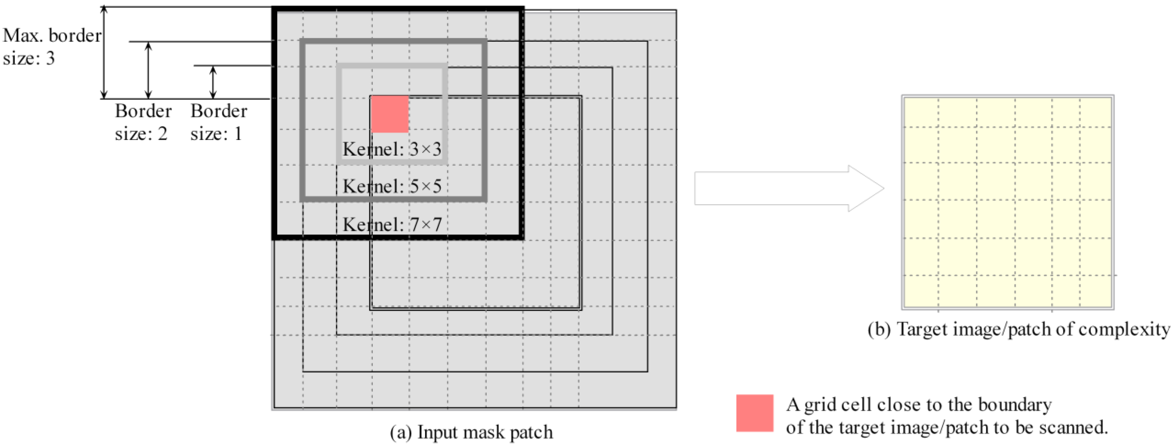
To achieve the efficient extraction of local surface complexity feature, we designed its convolution operator (Figure 1 and Figure 2a) and made full use of the GPU and parallelization of PyTorch’s deep learning software [60] to accelerate the complexity computing. In order to avoid the edge effects of complexity convolution computations [61], the input of the mask needed to contain additional class values within half the kernel size outside the boundary so that the complexity on the edge of the image or patch could be evaluated correctly. For multiscale complexity extraction, we used half of the maximum kernel size as the border size of the target mask patch so that the borders at the other scales could also be covered (Figure 1). Corresponding to the definition of the pixel-level entropy-based complexity, as aforementioned, the kernel of the complexity convolution is equivalent to the context surrounding the target point or location, and the size-varying kernels of complexity convolutions correspond to multiscale contexts surrounding the target pixels or locations. Given the scale dependence and multiscale effects [26] of surface complexity for remote sensing and geoscience applications, we proposed a multiscale surface complexity for the trained model to capture the invariance to scale variations [62].
While our definition of surface complexity is based on all pixels and classes in the local context, we focused on a binary classification in this manuscript. This was because, even for multiclass problems, combining binary classifiers often yields better performance than using a multiclass classifier alone [63,64,65]. Moreover, binary applications are typical and representative, and their labels often involve binary rather than multiclass labeling due to the high cost of data labeling. To make our approach widely applicable, we simplified the definition of surface complexity to binary classes (target class and background) and developed the application and technical evaluation route based on binary classification.
2.2. Learning Entropy-Based Multiscale Complexity
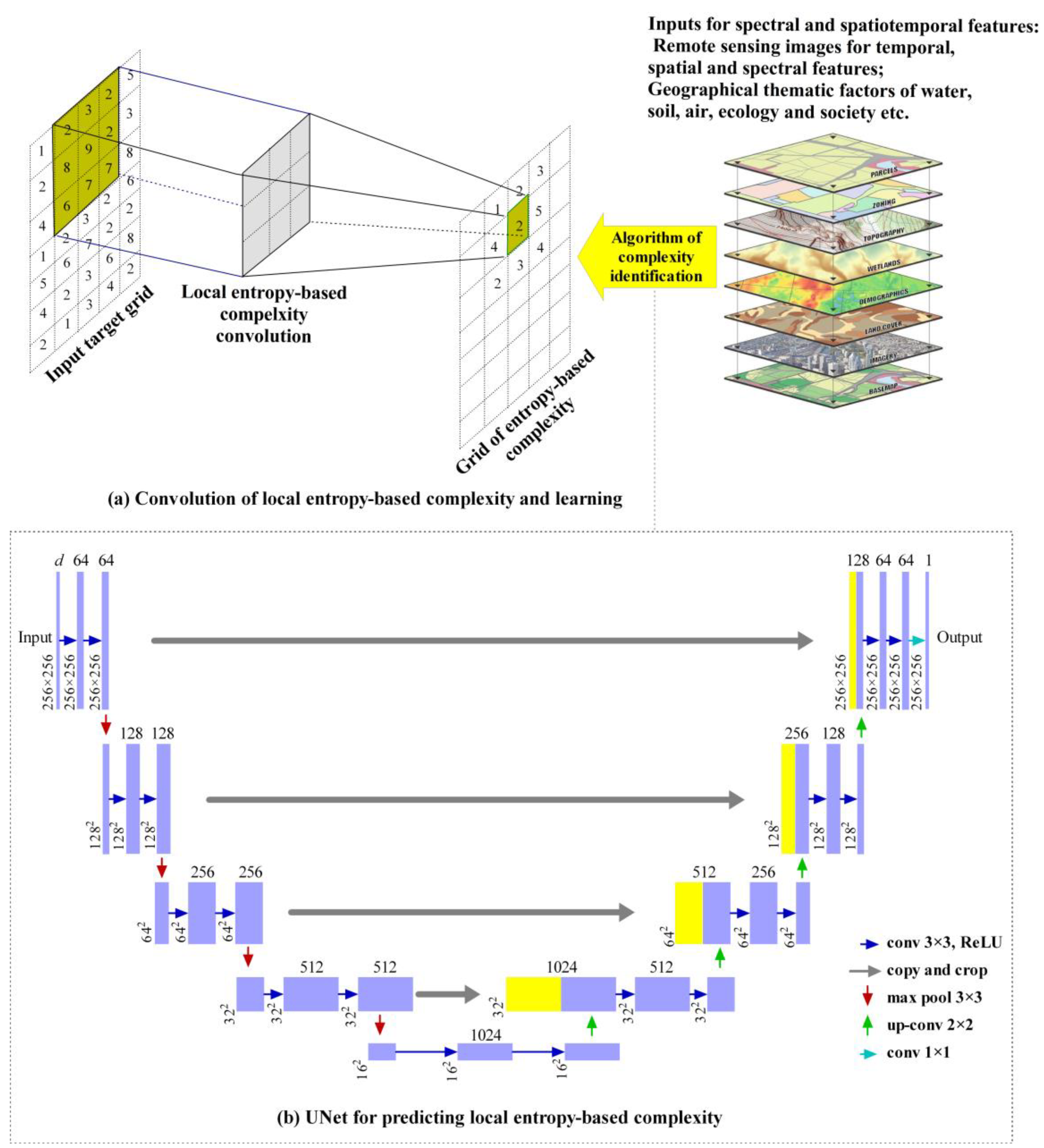
For the pixel-level entropy complexity extracted from the mask images of class labels, it is important to learn such local surface complexity based on the input of remote sensing spectral and/or spatiotemporal features. The learned model can be used to estimate the complexity at unobserved locations or regions. As aforementioned, surface complexity exhibits scale dependence, nonlinearity, and uncertainty, and it is influenced by multiple factors, including not only spectral properties but also geographic, ecological, and socioeconomic characteristics, etc. Therefore, to accurately capture local surface complexity, inputs in learning can include a variety of driving and influencing variables (Figure 2a).
Since local surface complexity is extracted using an entropy-based convolution operator, UNet is a natural method for learning the complexity, and its multi-convolutional encoder–decoder structure can encapsulate the surrounding context for the target pixel or spatial location of interest (Figure 2b). As a fully convolutional neural network, UNet has been widely used in various application fields such as medical image analysis, remote sensing, and industrial inspection since its launch in 2015 [66]. It consists of an encoder pathway that captures an image’s features at multiple scales and a corresponding decoder pathway that reconstructs the segmented image by upsampling. In UNet, skip connections between the encoder and decoder pathways facilitate the preservation of spatial information during the segmentation process. Compared with Unet, other machine learning methods such as random forest, XGBoost, and support vector machines do not have such a mechanism to model such a context. Sensitivity analysis has shown the low generalization of these methods in comparison with UNet. To improve the learning of our model, we added the layers of batch normalization, a ReLU activation function, and dropout after each convolution layer.
For the model learning and the optimization of local surface complexity scores, the mean squared error (MSE) loss function was used [67]:
where n is the number of samples, is the surface complexity computed from the binary mask within the kernel window for grid cell i, W denotes the parameters of the network (W = {wk}), is the surface complexity of grid cell i estimated by the network, K is the number of parameters in W, and is the weight for the L2 regularizer ().
The optimal hyperparameters including the learning rate (1 × 10⁻⁵ to 0.1), beta1 (0.1–0.9), beta2 (0.1–0.9), and the loss weight (λ) were obtained through grid search.
2.3. Complexity-Informed Optimal Sampling and Constrained Optimization
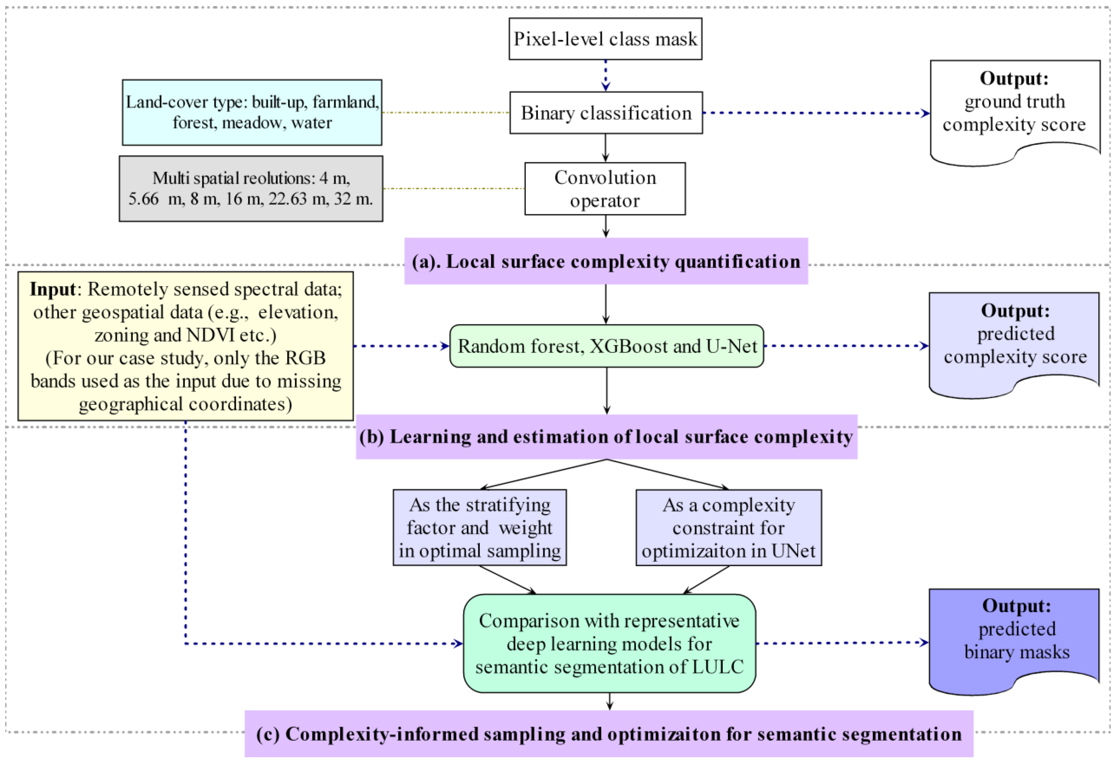
An important source of high uncertainty in remote sensing information extraction is sampling bias, where unrepresentative samples are selected for training and/or testing, especially since the majority of the bias usually arise from complex contexts [68,69]. Therefore, we used the average multiscale surface complexity as the stratifying factor and the sampling weight to increase the representativeness of the samples. For each stratum, the samples with high complex context could be selected with a high probability. Thereby, we could obtain more balanced samples for training and testing than simple random sampling [70]. In addition, the local surface complexity feature could be used as a constraint to strengthen the model training to tackle the classification and identification of the target objects under complex surface contexts. Figure 3 presents a flow chart for the local surface complexity quantification, learning, and optimal sampling and the constrained optimization for semantic segmentation. Figure 3 also shows the input and output for each of three phases in our method. In this study, we focused on the evaluation of local surface complexity for binary segmentation of land use and land cover using remotely sensed data.
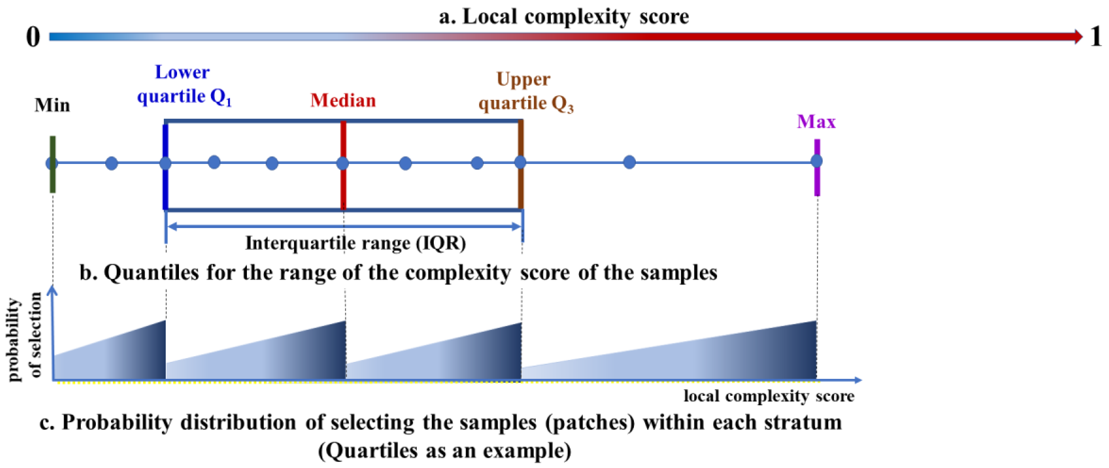
For the optimal sampling, the estimated complexity scores were first summarized, and the samples were stratified using the summed quartiles (or more quantiles), and then the same proportion was used in the sampling within each stratum, and the samples drawn in each stratum were combined into the training and test samples, respectively. Within each stratum, the local surface complexity score was used as the sampling weight, and the samples with high complexity scores were more likely to be selected for training (Figure 4). Therefore, the samples with different complexity scores were relatively evenly distributed in the training and testing samples, while the model could also focus on samples with high complexity scores in the learning to boost the generalization of the trained model. Selecting samples that are representative of the population is crucial to the learning of a segmentation or classification model, otherwise the learned model has sampling bias.
For the semantic segmentation of land use or land cover, the complexity scores extracted from ground truth data can be used as a constraint loss term to enhance model training. For binary segmentation, we used a combined loss function, which consisted of Dice loss (), binary cross-entropy (BCE) loss (), and the MSE loss of local surface complexity constraint (). The model outputted a 256 × 256 patch consisting of two bands, one representing the predicted probability of the target class and the other representing the estimated surface complexity score. The BCE loss was derived from the former, while the MSE loss was derived from the latter. The BCE loss is commonly used as a stable loss function for binary segmentation, as it is based on Bernoulli’s distribution loss. However, it may not perform well for highly imbalanced classification tasks. On the other hand, the Dice loss, which is inspired by the Dice coefficient score, is effective for learning better boundary representations, but its learning can be unstable for extremely imbalanced classifications. Thus, we leveraged the benefits of both the BCE and Dice losses to create a combined loss function [71] that is more appropriate for imbalanced samples, such as those encountered in land cover classification. Additionally, the combined loss function includes the complexity loss term to preserve the entropy-based invariance, thus mitigating overfitting.
where is the ground truth mask of the target class c, is the probability of belonging to the target class, c, predicted by the network, is the weight for the Dice loss, is the complexity extracted based on , is the estimated complexity by the same network, is the weight for the optional complexity loss, and is the smooth constant. With the surface complexity as an optimization constraint, the network needed to output two items, one being the binary prediction mask and the other being the estimated complexity.
3. Experiments
3.1. Dataset
To evaluate the proposed method, we used a large-scale land cover dataset with the Gaofen-2 (GF-2) satellite images (GID) and their reference annotations, which are publicly accessible (https://captain-whu.github.io/GID15 (accessed on 3 January 2022)) [72]. Gaofen-2 (GF-2) is the second satellite of the high-definition Earth observation system launched by the China National Space Administration (CNSA). GID provides multispectral images with a range of blue (0.45–0.52 μm), green (0.52–0.59 μm), red (0.63–0.69 μm), and near-infrared (0.77–0.89 μm) images and a spatial dimension of 6800 × 7200 pixels covering a geographic area of 506 km2. GF-2 images have a high spatial resolution (4 m used in this study) and wide field of view, allowing for detailed observation over large areas. We used the large-scale clarification set of GID, in which five major categories were annotated, namely build-ups, farmland, forest, meadow and waters, which were defined according to the Chinese land use classification criteria (GB/T21010-2017) [73]. The dataset contains 150 high-quality GF-2 images and labels from over 60 different cities in China, representing the distribution of ground objects in different areas, variations, and complex land surface scenes (see Figure 5 in [72] for the spatial distribution of the samples). With its rich diversity, GID could well be used to evaluate our proposed method of quantification, learning, and applicability of the local entropy-based surface complexity. GID does not provide latitude and longitude coordinates, so we could not extract any geospatial data, such as elevation or NDVI, to enhance the learning of local surface complexity and semantic segmentation.
3.2. Experimental Detail
Our experimental dataset consisted of 150 labeled images with an image size of 6800 × 7200 and a spatial resolution of 4 m. We considered two types of multiscale: one using multiple different kernel sizes, and another that upscales the original image at multiple spatial scales. For the former, we could extract the local surface complexity from the original images with different sized kernel contexts, which were most effective for geographic features with high local variations; for the latter, we could extract the local surface complexity from a wider convolutional field on the target object, which was most effective for geographic features with low local variation. For upscaled images, the extracted surface complexity was converted back to its original scale using bilinear resampling.
For the surface complexity convolution operation and UNet learning, the original or upscaled images were divided into multiple patches with the same resolution (s × s, s = 256 + b, b being the corresponding border size). For each of the five land covers, we extracted their binary masks and calculated their local surface complexity. In order to obtain a dataset of balanced samples, especially for the target features with a small distribution in GID, we calculated the pixel-level class count proportion for each patch and used it as a sampling weight so as to increase the probability of a patch with a high class proportion being selected. Of the selected images for a target class, 80% were used to train the model and the remaining 20% were used to test the model.
To quantify the local surface complexity, we extracted it from the binary mask input. For the learning of the surface complexity, we tested random forest, XGBoost, and UNet to check which had a better generalization ability. Since the GID dataset did not provide geographical coordinates, we only used the RGB bands of the images as the input bands to the learning models such as UNet, and no geographical variables were used. We then examined the applicability of the estimated local surface complexity for the optimal selection of the samples and for its use as a constraint in binary semantic segmentation. To conduct the independent test of binary semantic segmentation, we first randomly selected an image whose surface complexity score fell within the interquartile range of all the estimated scores and derived independent testing patch samples from it. Next, we used the stratified sampling strategy based on the estimated complexity scores to select patches from the remaining images for training and regular testing. We summarized the quantiles as the stratifying factor, using the mean complexity scores of all the remaining patches, and we also used the complexity scores as a weight factor to randomly select 80% of the patches in each stratum for the training samples and the remaining 20% for the regular testing samples, as shown in Section 2.3 and Figure 4. Finally, we combined the training samples from all the strata to train the model and combined the testing samples for regular testing. The surface complexity score played a crucial role in the sampling and selection of samples in the training, regular testing, and independent testing. This ensured balanced samples were obtained in the selection and reduced selection bias.
3.3. Training
The training dataset comprised about 3000 RGB image patches, each with a size of 276 × 276. This size included the target output size (256 × 256) along with a maximum border size of 10 pixels on each side to eliminate boundary effects during the surface complexity estimation and semantic segmentation. The input bands were normalized by dividing by 255. The output patch size for both the surface complexity estimation and the binary semantic segmentation was set at 256 × 256. To obtain sufficient patch samples, oversampling was conducted for positive instances and undersampling for negative instances, with the estimated surface complexity serving as the stratifying and weighing factor. The over- and undersampling distances were determined based on the number of positive instances [61]. The models were trained for 160 epochs using the Adam optimizer with the Nesterov momentum. The initial learning rate was set to 0.001 and was adaptively adjusted during the learning process. The mini-batch size of patches was set to 10, and an early stopping criterion was employed during the training.
3.4. Evaluation and Prediction
We used two common metrics for continuous predictors, R-squared (R2) and root mean squared error (RMSE), to measure the performance of the learned models in estimating the local surface complexity.
- (1)
- R2 can be defined as:where is the observed complexity computed from the ground truth data (binary mask), is the complexity estimated by the learned model, denotes the mean of the observed complexity, n is number of samples, TSS denotes the total sum of squares (=), RSS denotes the residual sum of squares (=), and ESS denotes the explained sum of squares ().
- (2)
- RMSE can be defined as:
For binary semantic segmentation, we used the following performance metrics:
(1) The pixel accuracy (PA), which is defined as the ratio of the number of correctly classified pixels to the total number of pixels:
where C denotes the number of classes, is the total number of pixels correctly classified as class k, and denotes the total number of pixels labeled as class k.
(2) The intersection-over-union (IoU), also known as the Jaccard index (JI), which is defined as the size of the intersection divided by the size of the union of the sample sets and is to measure the degree of overlap between two frames. It is the most popular evaluation metric for segmentation.
where is the set of ground truth masks, is the set of predicted results, is the total number of pixels correctly classified as target class c, is the total number of pixels whose ground truth is class i and is classified into target class c, and is the total number of pixels whose ground truth is class c and is classified into target class i.
(3) The mean intersection-over-union (MIoU), which is defined as the average of the IoU or JI of all classes:
PA is a metric that is easy to understand and use, but it is not the best metric for segmenting class imbalance since it can be dominated by the majority classes and may not accurately reflect the test performance for the minority classes. Compared to metrics such as PA, Kappa, and F1-score, the IoU or JI is one of the most commonly used metrics in semantic segmentation. It is a straightforward and effective metric, particularly for unbalanced segmentation tasks such as land use or land cover classification with complex contexts. The MIoU provides a comprehensive metric for all classes as the average IoU and is particularly effective for unbalanced classification tasks. For pixel-level semantic segmentation, we selected simple PA as well as the most effective IoU and MIoU as the performance metrics, since together, they provide a comprehensive measure with effective evaluation for unbalanced classification.
After the models were trained, they were used to make predictions. For large-sized image prediction, the image was first divided into patches of size 276 × 276 with a slight overlap between adjacent patches. The input bands were normalized by dividing by 255 and then used as the input to the trained models for prediction. The output patch size was set at 256 × 256, and all the predicted patches were merged by taking the mean of the predicted values (surface complexity scores or predicted probabilities of the target class) for the overlapping areas. The final prediction excluded the boundary (10 pixels on each side) of the image to eliminate boundary effects.
In order to illustrate the generalization of our method, we compared our results with those of four representative deep learning methods, including FCN ResNet, global CNN, DeepLab V3+, and Crossformer. The four representative methods developed new network structures to enhance the information extraction of semantic boundaries: FCN-ResNet was constructed by a fully convolutional network model using a ResNet (ResNet-101 for our comparison case) backbone [42]; Global CNN utilized a large kernel to help perform the classification and localization tasks simultaneously [43]; DeepLab V3+ combined an atrous spatial pyramid pooling block (ASPP) and depth-wise separable Xception architecture to obtain a faster and stronger network [45]; and Crossformer proposed two designs of a cross-scale embedding layer and a long short distance attention to achieve cross-scale attention [47]. To compare with these methods, we used simple random sampling rather than complexity-informed optimal sampling to obtain the training and test samples.
4. Results
4.1. Quantification of Local Surface Complexity
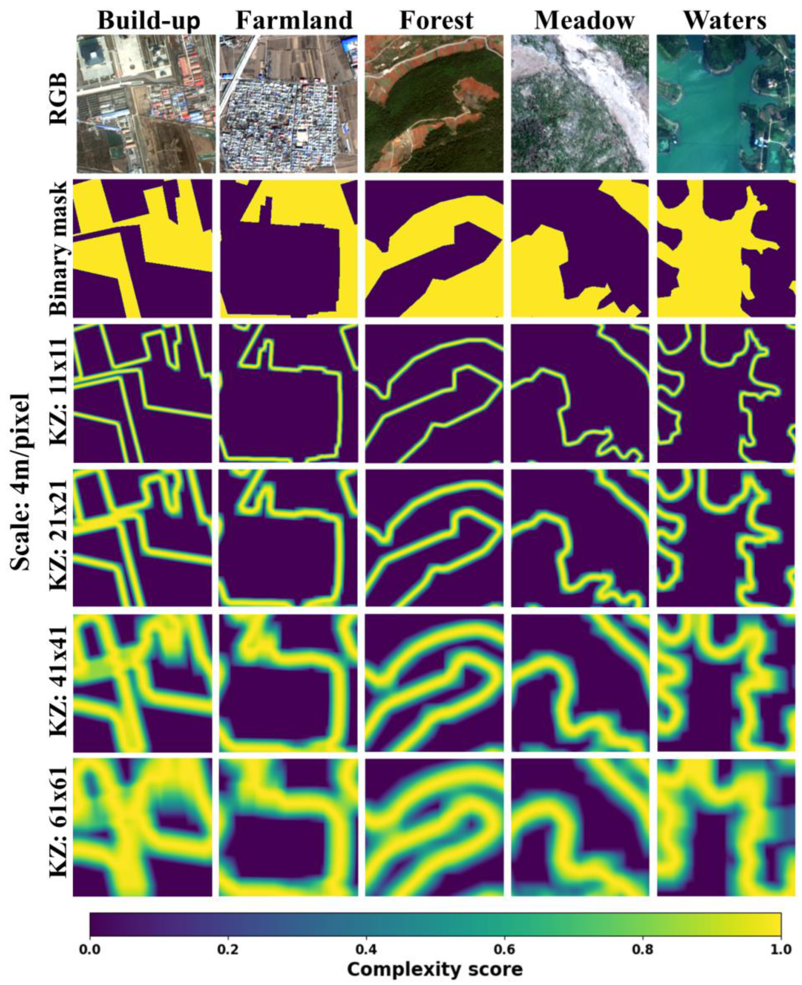
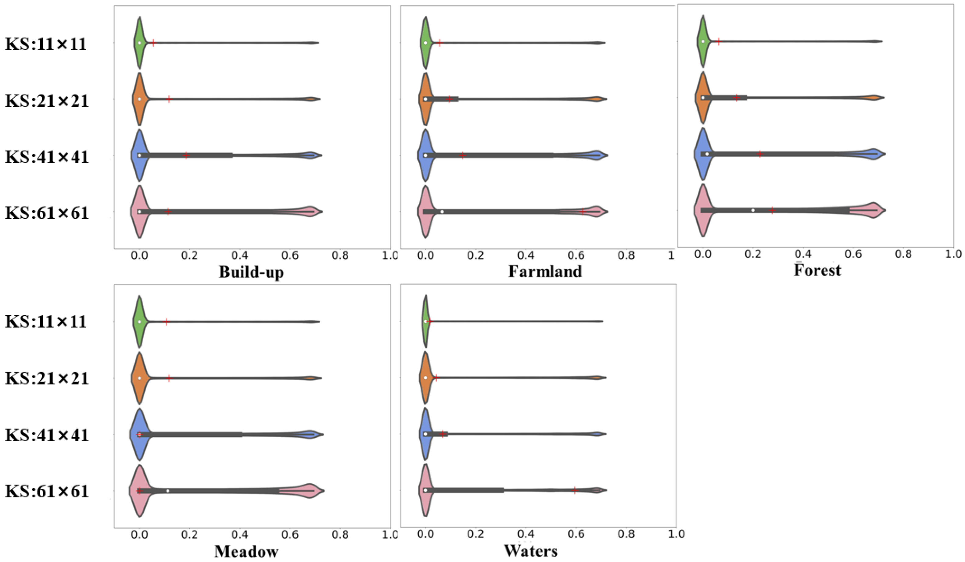
Using different kernel sizes, namely 11 × 11, 21 × 21, 41 × 41, and 61 × 61, we obtained the multiscale local surface complexity for each of the five land cover types (build-ups, farmland, forest, meadow, and waters) (Figure 5). We summarized their statistical violins (Figure 6). For the 11 × 11 scale, we extracted the fine-scale surface complexity, which exhibited high values at the edges of the binary mask, as shown. Since the edges, especially at the mask corners or intersections, varied widely or sharply, they naturally had a high local surface complexity. As the kernel size varied from 11 × 11 to 61 × 61, the extracted surface complexity exhibited a wider context and a more gradual change.
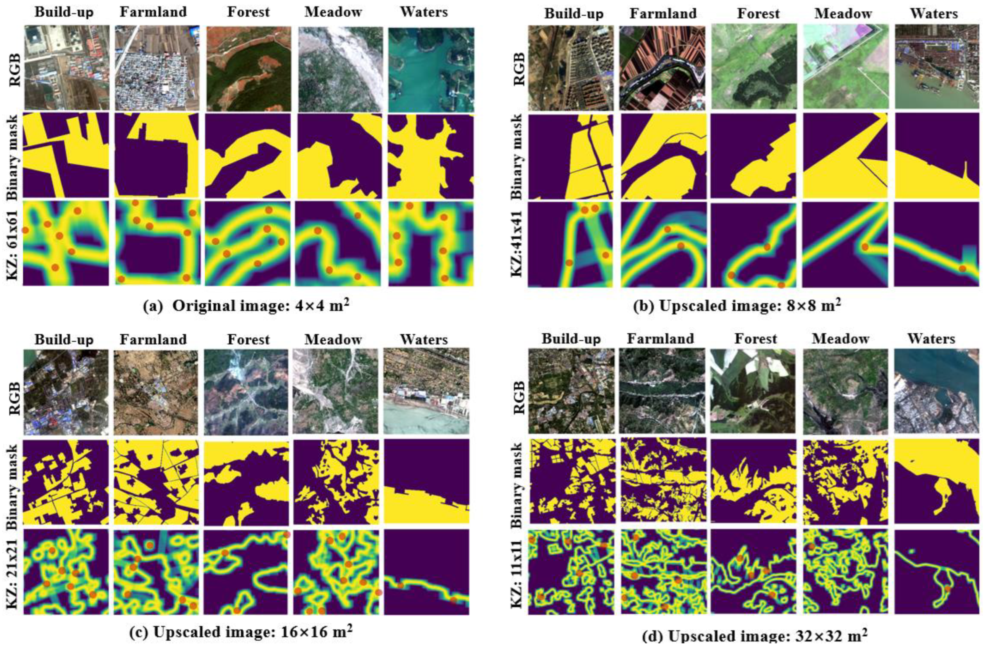
In order to make the view field of the local surface complexity convolution increasingly wider, we also upscaled the original image to three different spatial resolutions, i.e., 8 × 8 m2, 16 × 16 m2, and 32 × 32 m2. Four different kernel sizes were set up for the original and upscaled images: 61 × 61 for 4 × 4 m2, 41 × 41 for 8 × 8 m2, 21 × 21 for 16 × 16 m2, and 11 × 11 for 32 × 32 m2. The entropy-based surface complexity was extracted for each land cover (Figure 7). The results presented different patterns and hotspots of local surface complexity. We conducted a simple grid search empirically to determine the configurations for upscaling and kernel sizes. Utilizing these configurations, we computed multiscale surface complexity scores, which led to a significant enhancement in the segmentation performance as compared to the baseline models that did not employ surface complexity scores.
4.2. Learning of Local Surface Complexity
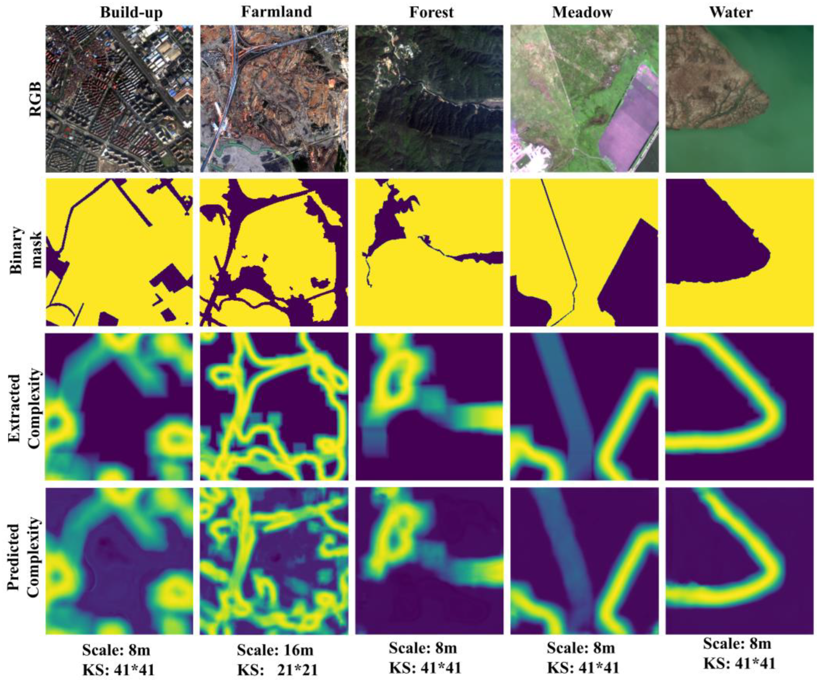
We used random forest, XGBoost, and UNet to learn the models for predicting the local surface complexity. The sensitivity analysis demonstrated that UNet increased the test performance (test R2) by over 50% when compared to random forest and XGBoost. Since the entropy-based surface complexity scores were computed using convolutional kernels, UNet, based on convolutional operators, was a natural way to learn the local surface complexity score. In contrast, random forest, XGBoost, and support vector machine, etc., cannot explicitly model neighborhoods unless such contextual information is encoded into the input using the nearest neighbor method. Table 1 and Table 2 display the R2 and RMSE performance metrics for the trained UNet, XGBoost, and random forest, utilizing varying upscales (4 × 4 m2, 8 × 8 m2, 16 × 16 m2, and 32 × 32 m2) and kernel sizes (61 × 61, 41 × 41, 21 × 21, and 11 × 11), respectively. For the upscales > 4 × 4 m2, the results showed a high test R2 (0.826–0.969) for build-ups, forest, meadow, and waters and a moderate test R2 (0.560–0.751) for farmland. For the original image resolution (4 × 4 m2, kernel size: 61 × 61), there was a lower test R2 (0.414–0.738) than the upscales. Compared with farmland, the local surface complexity scores of build-ups, forest, meadow, and waters were more predictable using only spectral features. Overall, the local surface complexity scores could be estimated using spectral features and UNet, although the predictability varied between the different land cover classes. The results (Figure 8) showed that the estimated scores well captured the local surface complexity of each land cover class.
4.3. Optimal Sampling and Constraints for Land Cover Segmentations
Based on the multiscale surface complexity scores with different upscales and kernel sizes (Table 1), we first rescaled the upscaled scores into the original scale (4 × 4 m2) using bilinear resampling and then summarized their averages. As aforementioned (Figure 4), the estimated complexity scores were used as the stratification and weighting factors to guide the balanced selection of samples to reduce the sampling bias. In addition, the complexity scores extracted from the ground truth data were used as a constraint (Equation (4)) in the loss function to guide the optimization. For the baseline UNet, we considered the network complexity and test accuracy to determine its architecture (the network depth and the number of nodes for each layer). Through sensitivity analysis, we selected the UNet architecture ([64, 128, 256, 512, 1024, 2048, 1024, 512, 256, 128, 64] for build-ups and farmland; [32, 64, 128, 256, 512, 1024, 512, 256, 128, 64, 32] for forest, meadow, and waters) with a relatively high test performance and less training time. Then, based on the baseline UNet, we tested the effectiveness of the complexity-informed sampling and constrained optimization on the generalization of the trained models.
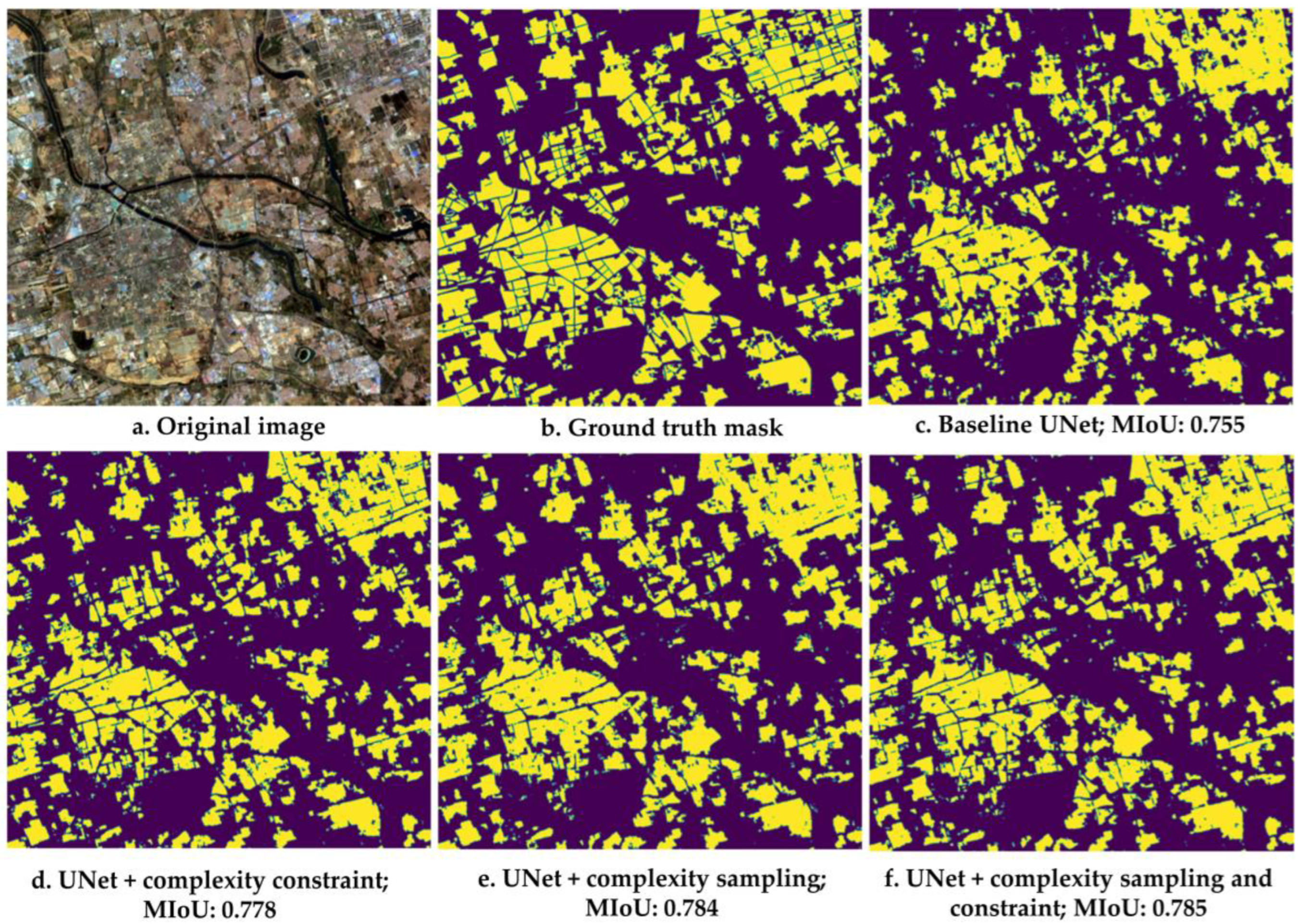
The build-up land cover included the subcategories of industrial land, urban residential, rural residential, and traffic land [72]. The results showed that the complexity-informed sampling outperformed the baseline UNet in terms of the regular test JI and PA by 3.00% and 2.10%, respectively (Table 3). Moreover, the constraint approach improved the regular test JI and PA by 2.40% and 1.60%, respectively. Based on UNet, the combination of complexity-informed sampling and constrained optimization had the largest improvement (JI by 4.00% and PA by 2.90% for regular testing). Figure 9 and Table 3 show the image-based independent test results of build-up segmentation, where complexity-informed sampling and constrained optimization improved JI by 2.70% and 2.10%, respectively, when compared to baseline UNet. Together, the two improved the JI by 3.10%. The results showed that while complexity-informed sampling improved the representativeness of the samples to the population, the complexity constraint enabled the trained model to better recognize the boundary between smaller different build-up land patches.
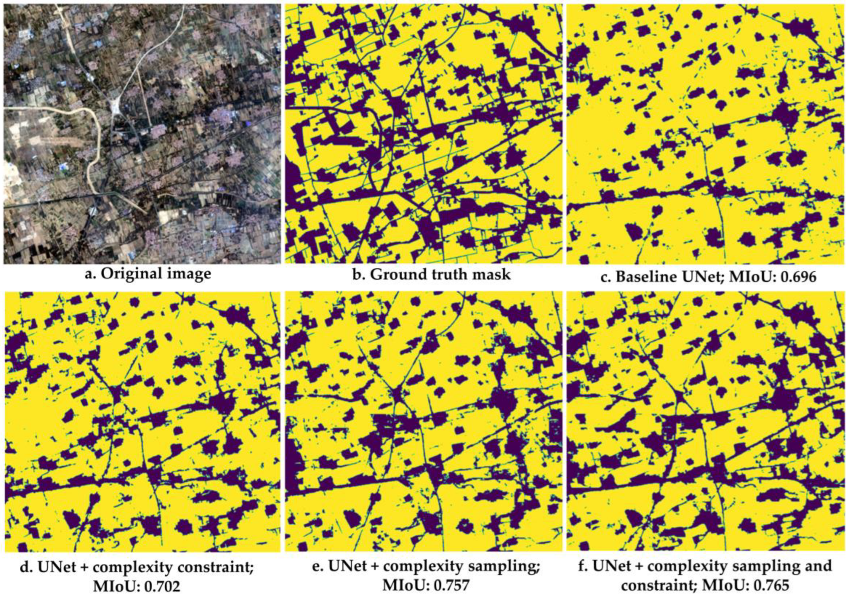
In the GID data, the morphology of the build-up land and farmland varied greatly due to the diversity of the geographic locations [72], making their segmentation challenging compared to the other land cover types (forest, meadow, and waters) [20]. The results (Table 3) showed that complexity-informed sampling had the greatest improvement in regular test JI (by 9.10%) and MIoU (by 10.70%) for farmland (including paddy fields, irrigated land, and drop cropland) compared to the other land cover types, although the improvement in the regular test PA was only 1.80%. The complexity constraint alone yielded a 0.90–1.10% improvement in the test PA and JI. Overall, the two improved the JI by 10.40% and PA by 1.90% compared to the baseline UNet. Given the changes in farmland morphology, particularly in its seasonal fallow and alternatives, it is crucial to choose representative samples from various geographical locations and seasons to reduce sampling bias. This also explained why the complexity-informed sampling by stratifying and weighing contributed most to the improvement in the JI compared to the other land cover types. The image-based independent test results (Figure 10) showed an improvement of about 5.30% in the JI by combining complexity-informed sampling and constraint.
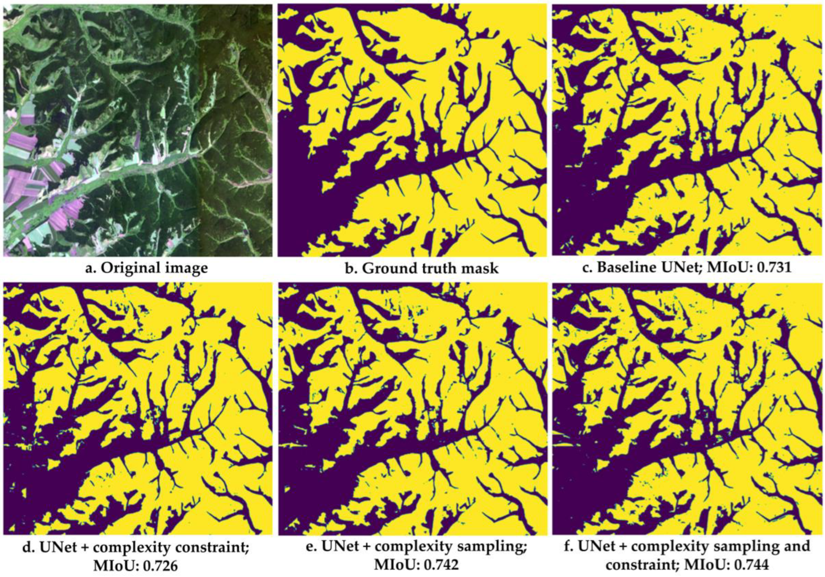
For the forest land cover (including garden land, arbor forest and shrub land), the complexity constraint had an improvement of about 1.30% in the regular test JI. The complexity-informed sampling provided little contribution to the test performance. The combination of the two resulted in an improvement of 2.30% for the regular test JI (1.90% for MIoU). The image-based independent test results (Figure 11) showed an improvement of about 1.70% in the JI compared to the predictions of the baseline UNet.
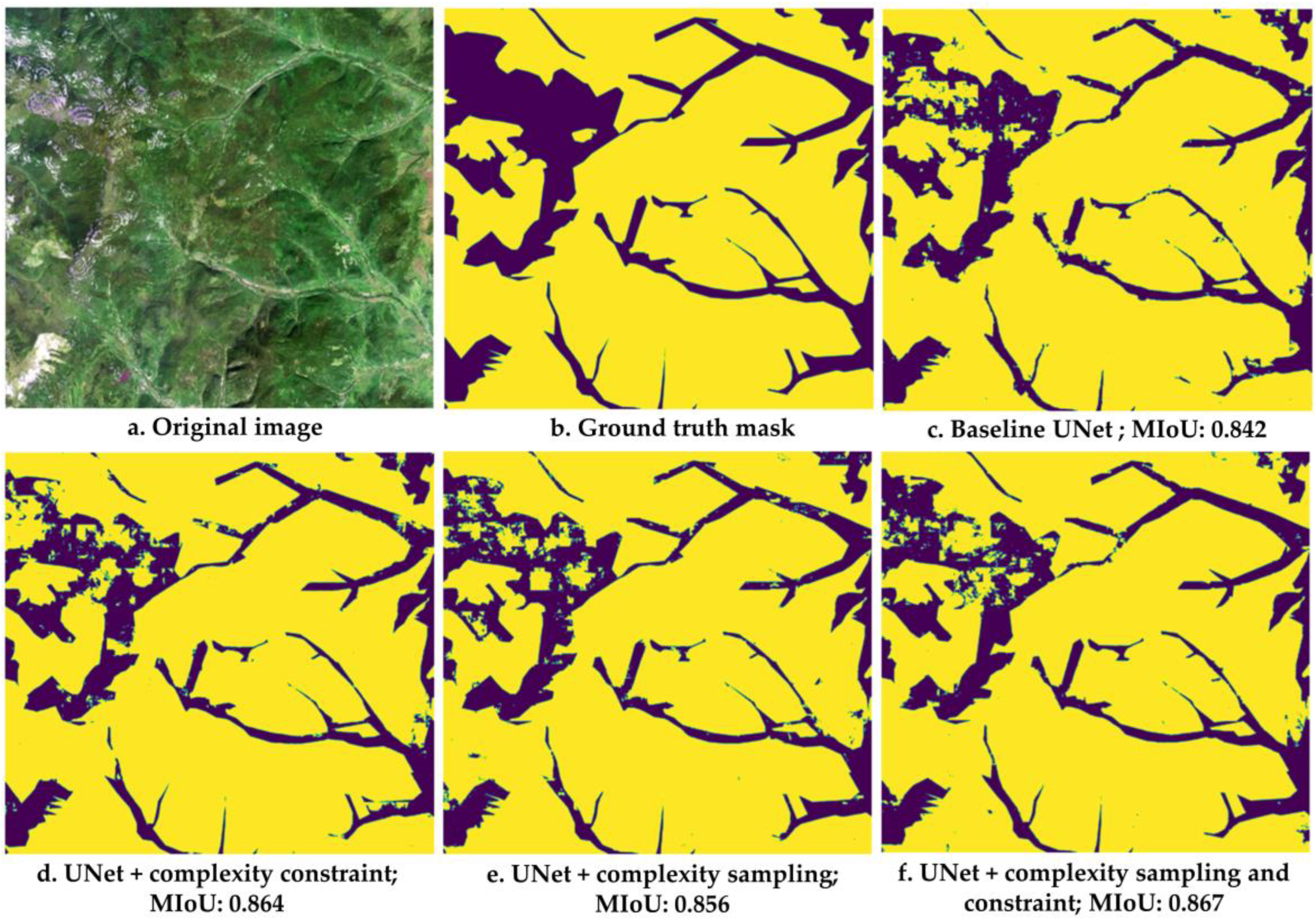
For the land cover of natural and artificial meadows, the complexity constraint had an improvement of about 0.90% in the test JI (about 1.20% for MIoU) when compared to the baseline model. The combination of complexity-informed sampling and constraint improved the regular test JI by about 1.00%. The image-based independent test results (Figure 12) showed an improvement of about 2.60% in the JI.
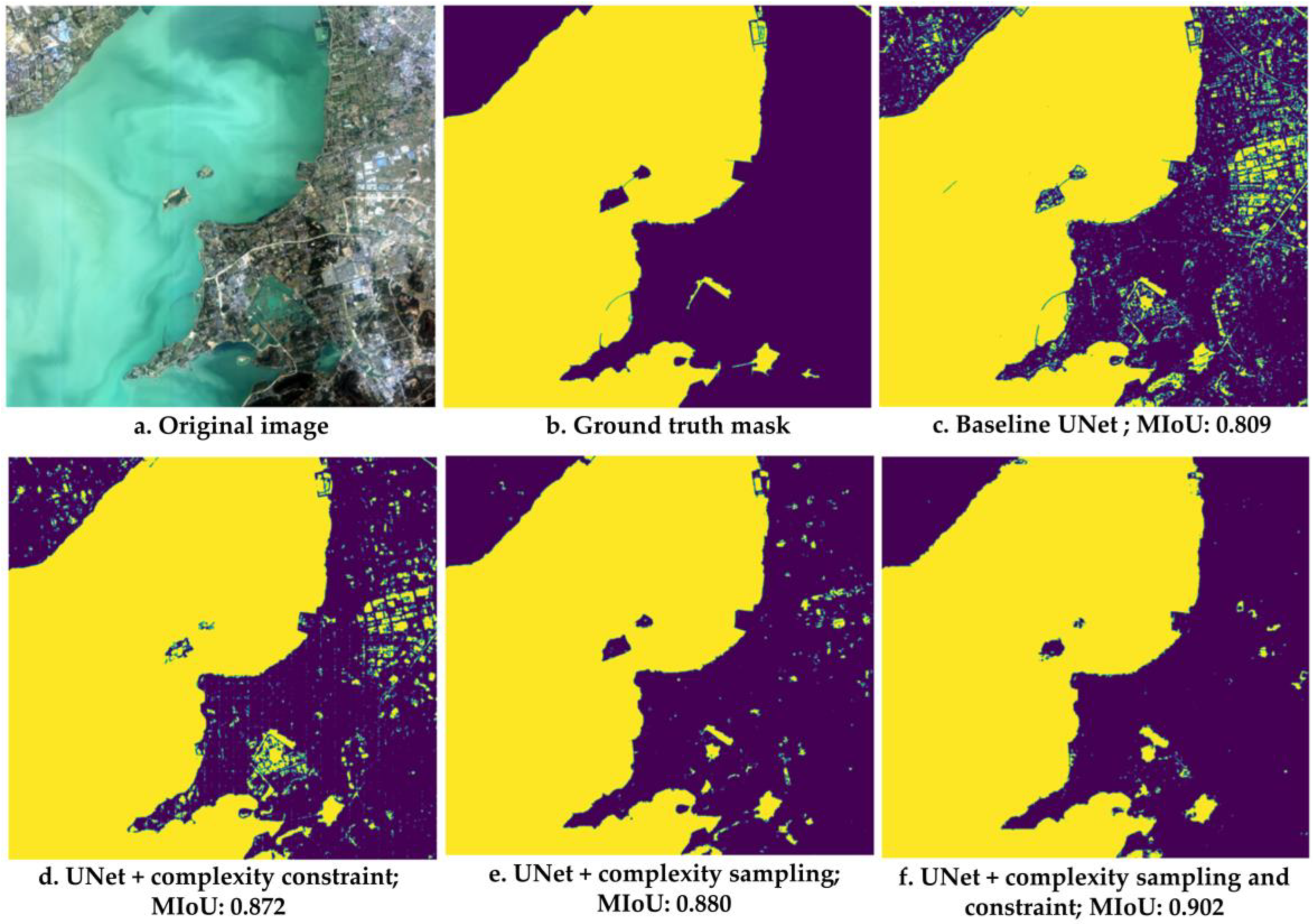
For waters (including rivers, ponds, and lakes), the complexity constraint had an improvement of about 0.20-0.80% in the regular test PA, JI, and MIoU. The combination of complexity sampling and constraint had an improvement of about 1.30% for the regular test JI. The image-based image results (Figure 13) showed a considerable improvement of about 8.00% in the JI. As shown in the figure, many misclassified waters were corrected from the UNet by complexity sampling and constrained optimization.
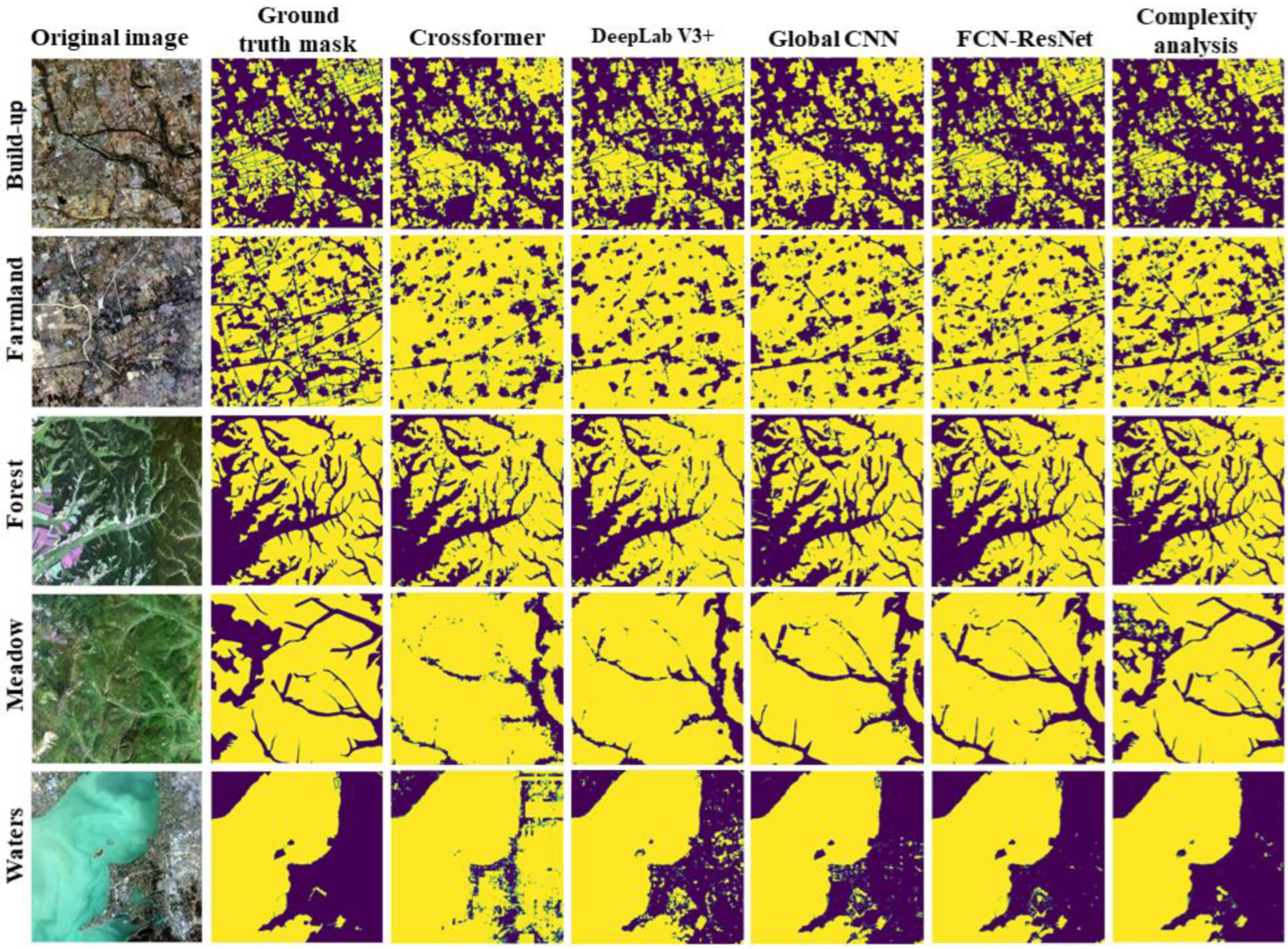
The tests (Table 4) showed that our complexity analysis method outperformed FCN-ResNet, DeepLab V3+, Global CNN, and Crossformer in terms of the regular test PA and JI for the semantic segmentation of farmland, forest, meadows, and waters. Notably, our method achieved significantly better test JI results for farmland than the other methods, indicating the importance of reducing sampling bias in training for variable farmland. While our method performed better than DeepLab V3+ and Crossformer for the semantic segmentation of build-ups, its PA was slightly lower than FCN-ResNet and Global CNN. Furthermore, our method achieved comparable state-of-the-art test performances in the image-based independent tests when compared to the other representative methods (Figure 14).
5. Discussion
5.1. Optimal Sampling to Reduce Bias
Previous studies [53,55,56,74,75,76,77] have shown that stratification can balance samples across regions, leading to an improved classification accuracy. Li et al. (2021) [53] suggested that stratifying with land cover classes or a combination of different attributes considerably improved classification. Shetty et al. (2021) [78] showed that stratified equality, proportional, or systematic random sampling performed differently in different situations. Compared with these existing studies relying on unsupervised stratifying with a land use or land cover classification or combined attributes, our study suggested the use of a quantitative local surface complexity score as the stratifying and weighing factor to boost the representativeness and importance of the training samples to the complexity of the features of the Earth’s surface. The statistical data showed that the complexity-informed sampling method significantly improved the test JI (by up to 9.10%), with a more pronounced effect being obtained on farmland and urban built-up areas where the boundaries varied greatly. Despite being based on the baseline UNet framework, our complexity analysis method achieved a state-of-the-art test performance for the LULC semantic segmentation of the GID dataset in comparison with four representative deep learning methods including FCN-ResNet, DeepLab V3+, global CNN, and Crossformer. A reasonable explanation is that, compared to simply random sampling, the extracted local surface complexity as stratifying factor better balanced the distribution of the samples among the different surface complexity degrees, and the selected samples could represent the complexity of the features of the Earth’s surface. In addition, samples with higher complexity scores in each stratum had a higher probability of being selected, so the learning model could pay more attention to the samples with a higher complexity. Thereby, the sampling bias was reduced significantly and consistently, and the visual output also showed that the fine irregularities in the classification were also captured using more balanced and representative samples. If selected samples cannot adequately represent the complexity of a population under study, a potential sampling bias can significantly impact the test performance of deep learning methods even though they have developed novel network structures, as shown in our results.
Based on spectral attributes, we developed a robust model that learned to estimate surface complexity. The trained model can be used to reliably estimate the surface complexity for new locations or regions where the land use or land cover classification is not available. For optimal sampling, this is an important advantage of our quantifying stratification based on surface complexity compared to the existing methods that rely on land cover classification or a priori knowledge to stratify the samples. Given the high cost of labeling of remote sensing images and the critical impact of the samples on training, this study provides a systematic and comprehensive cost-effective sampling strategy to improve the representativeness of the samples to complex populations.
5.2. Constrained Optimization to Reduce Overfitting
Traditional machine learning methods such as logistic regression, random forest, and support vector machine have no internal mechanisms for constrained optimization. With the widespread applications of deep learning in remote sensing, constrained optimization has been increasingly used in loss functions to reduce modeling bias and overfitting [79]. Teng et al. (2019) [80] proposed a classifier-constrained deep adversarial domain adaptation method for cross-domain classification in remote sensing images. The study showed that overfitting could be significantly reduced by constrained optimization. In this study, we proposed the invariance of the extracted entropy-based complexity score as the constraint for optimization. The model could output a classification score and a complexity score for each pixel, and the architecture enabled the parameter sharing of the network for the classification and complexity prediction. This constraint guided the learning of the classification model considering the invariance of the complexity feature, which was beneficial for reducing modeling bias and potential overfitting. The test showed that the complexity constraint improved the test JI by 0.30–2.40% and could help the learned model to better extract the boundaries between small complex land patches such as build-ups.
5.3. Combination of Optimal Sampling and Constrained Optimization
As demonstrated by the tests, the combined use of complexity-informed stratified sampling and constrained optimization performed the best (1.00–10.40% improvement in the JI and 0.30–2.90% improvement in the PA for the regular test; 1.70–8.00% improvement in the JI for the image-based independent test). The greatest improvement (the regular test JI of 4.00–10.40%) was observed for the classes that were more challenging to predict, such as build-up and farmland, with varying boundaries and irregularities. In this study, unlike in [20,44,81], we did not develop novel network structures of semantic segmentation but rather combined the use of multiscale local surface complexities in sampling and optimization to achieve the state-of-the-art test performance. Optimal sampling allowed us to have more balanced samples to represent the population surface complexity, which in turn could facilitate constrained optimization to reduce the sampling and modeling bias, thus improving the identification and extraction of complex boundaries, fragments, and tiny features, etc.
5.4. Limitations and Prospects
The study has several limitations. Firstly, the entropy-based surface complexity only considered binary classification, which may have overlooked the potential impact of other classes on the target class within the surrounding context despite the significant contributions it made to improving the binary segmentation via optimal sampling and constrained optimization. Secondly, the entropy-based surface complexity only took into account the pixel proportions of the target class and background without considering their spatial distribution or pattern. This may have been suboptimal for certain surface scenes. Thirdly, due to the impracticality of the fine-scale grid search optimization, we chose multiple scales of surface complexity scores through empirical methods. Lastly, the absence of geographical coordinate data in the GID dataset prevented us from including geospatial variables, which could significantly improve the predictions of local surface complexity and, consequently, semantic segmentation.
Given the challenges of remote sensing information extraction under complex surface scenes and the limitations of this study, we propose several avenues for future research. Firstly, we will explore more spatially informative convolutional kernels of complexity, such as Moran’s I or Getis’s G from spatial statistics, which can identify differences in the spatial distributions of classes among pixels. Secondly, we will investigate the influence of multiclass surface complexity on the classification of the target pixel or location. Thirdly, we will aim to incorporate other datasets with accurate geographical coordinates to investigate the influence and contributions of geographical variables, such as elevation and historic land use or land cover, on predictions of surface complexity and their applicability. Finally, we will continue to refine our proposed framework (including scale sizes) of local surface complexity to improve its visual effects, accuracy, and applicability in a wider range of remote sensing scenarios and the other novel machine learning methods.
6. Conclusions
In this research, we proposed entropy-based multiscale convolutions to encode local surface complexity at the fine-scale pixel level and developed complexity-informed sampling and optimization to enhance semantic segmentation under complex geo-scenes. Such complexity convolution as a context indicator could well summarize the surrounding variation and influence on the target locations or regions. Correspondingly, we developed a robust UNet to map the relationship from spectral features to multiscale surface complexity, which provided the method with a high flexibility and wide applicability to new locations or regions where no a priori knowledge or labels are available. As described and shown in the tests using the large-scale land cover dataset, GID, the proposed multiscale surface complexity could be used to obtain optimal samples to better represent the surface complexity of the population, thereby significantly reducing the sampling bias in the model training, as well as to guide the model optimization as an entropy-based invariance constraint. The combined use of multiscale local surface complexity in the sampling and optimization significantly improved the classification performance (the regular test JI was improved by 1.00–10.40%), achieving a state-of-the-art test performance in comparison with other representative deep learning methods. Our study offers novel insights and efficient ways for selecting representative samples from remote sensing data and reducing over-fitting. These findings have important implications for improving the effectiveness of remote sensing information extraction, particularly in complex surface scenes.
Author Contributions
Conceptualization, L.L. and Z.Z.; methodology, L.L., Z.Z. and C.W.; software, L.L. and Z.Z.; validation, Z.Z. and L.L.; investigation, L.L.; resources, Z.Z. and C.W.; data curation, Z.Z.; writing—original draft preparation, L.L.; writing—review and editing, L.L., Z.Z. and C.W.; visualization, Z.Z. and L.L.; supervision, L.L.; project administration, L.L.; funding acquisition, L.L. and C.W. All authors have read and agreed to the published version of the manuscript.
Funding
This research was funded by the National Key Research and Development Program of China (grant number 2021YFB3900501), National Natural Science Foundation of China (grant number 42071369), LREIS Independent Innovation Project (05Z5006JYA), and the Strategic Priority Research Program of Chinese Academy of Sciences (grant number XDA19040501).
Data Availability Statement
Data related to this article are available upon request to the corresponding authors.
Acknowledgments
The support of NVIDIA Corporation with the donation of the Titan Xp GPUs used for this research.
Conflicts of Interest
The authors declare no conflict of interest.
References
- Emery, B.; Camps, A. Introduction to Satellite Remote Sensing: Atmosphere, Ocean, Land and Cryosphere Applications; Elsevier: Amsterdam, The Netherlands, 2017. [Google Scholar]
- Managi, S.; Wang, J.; Zhang, L. Research progress on monitoring and assessment of forestry area for improving forest management in China. For. Policy Econ. 2019, 1, 57–70. [Google Scholar] [CrossRef]
- Li, M. Dynamic monitoring algorithm of natural resources in scenic spots based on MODIS Remote Sensing technology. Earth Sci. Res. J. 2021, 25, 57–64. [Google Scholar] [CrossRef]
- Xue, T.; Zheng, Y.X.; Geng, G.N.; Zheng, B.; Jiang, X.J.; Zhang, Q.; He, K.B. Fusing Observational, Satellite Remote Sensing and Air Quality Model Simulated Data to Estimate Spatiotemporal Variations of PM2. 5 Exposure in China. Remote Sens. 2017, 9, 221. [Google Scholar] [CrossRef]
- Zhao, S.; Wang, Q.; Li, Y.; Liu, S.; Wang, Z.; Zhu, L.; Wang, Z. An overview of satellite remote sensing technology used in China’s environmental protection. Earth Sci. Inform. 2017, 10, 137–148. [Google Scholar] [CrossRef]
- Reba, M.; Seto, K.C. A systematic review and assessment of algorithms to detect, characterize, and monitor urban land change. Remote Sens. Environ. 2020, 242, 111739. [Google Scholar] [CrossRef]
- Weiss, M.; Jacob, F.; Duveiller, G. Remote sensing for agricultural applications: A meta-review. Remote Sens. Environ. 2020, 236, 111402. [Google Scholar] [CrossRef]
- Ma, L.; Liu, Y.; Zhang, X.L.; Ye, Y.X.; Yin, G.F.; Johnson, B.A. Deep learning in remote sensing applications: A meta-analysis and review. ISPRS J. Photogramm. Remote Sens. 2019, 152, 166–177. [Google Scholar] [CrossRef]
- Zhang, L.P.; Zhang, L.F.; Du, B. Deep Learning for Remote Sensing Data A technical tutorial on the state of the art. IEEE Geosci. Remote Sens. Mag. 2016, 4, 22–40. [Google Scholar] [CrossRef]
- Zhu, X.X.; Tuia, D.; Mou, L.C.; Xia, G.S.; Zhang, L.P.; Xu, F.; Fraundorfer, F. Deep Learning in Remote Sensing. IEEE Geosci. Remote Sens. Mag. 2017, 5, 8–36. [Google Scholar] [CrossRef]
- Ghamisi, P.; Rasti, B.; Yokoya, N.; Wang, Q.; Hofle, B.; Bruzzone, L.; Bovolo, F.; Chi, M.; Anders, K.; Gloaguen, R. Multisource and multitemporal data fusion in remote sensing: A comprehensive review of the state of the art. IEEE Geosci. Remote Sens. Mag. 2019, 7, 6–39. [Google Scholar] [CrossRef]
- Gu, Y.; Liu, T.; Gao, G.; Ren, G.; Ma, Y.; Chanussot, J.; Jia, X. Multimodal hyperspectral remote sensing: An overview and perspective. Sci. China Inf. Sci. 2021, 64, 1–24. [Google Scholar] [CrossRef]
- Balsamo, G.; Agusti-Parareda, A.; Albergel, C.; Arduini, G.; Beljaars, A.; Bidlot, J.; Bousserez, N.; Boussetta, S.; Brown, A.; Buizza, R.; et al. Satellite and In Situ Observations for Advancing Global Earth Surface Modelling: A Review. Remote Sens. 2018, 10, 2038. [Google Scholar] [CrossRef]
- Fisher, R.A.; Koven, C.D. Perspectives on the future of land surface models and the challenges of representing complex terrestrial systems. J. Adv. Model. Earth Syst. 2020, 12, e2018MS001453. [Google Scholar] [CrossRef]
- Kaplan, G.; Avdan, U. Monthly Analysis of Wetlands Dynamics Using Remote Sensing Data. ISPRS Int. J. Geo-Inf. 2018, 7, 411. [Google Scholar] [CrossRef]
- Wen, J.G.; Liu, Q.; Xiao, Q.; Liu, Q.H.; You, D.Q.; Hao, D.L.; Wu, S.B.; Lin, X.W. Characterizing Land Surface Anisotropic Reflectance over Rugged Terrain: A Review of Concepts and Recent Developments. Remote Sens. 2018, 10, 370. [Google Scholar] [CrossRef]
- Xu, L.; Herold, M.; Tsendbazar, N.-E.; Masiliūnas, D.; Li, L.; Lesiv, M.; Fritz, S.; Verbesselt, J. Time series analysis for global land cover change monitoring: A comparison across sensors. Remote Sens. Environ. 2022, 271, 112905. [Google Scholar] [CrossRef]
- Zhang, J.; Zhao, R.; Shi, Z.; Zhang, N.; Zhu, X. Bayesian Constrained Energy Minimization for Hyperspectral Target Detection. IEEE J. Sel. Top. Appl. Earth Obs. Remote Sens. 2021, 14, 8359–8372. [Google Scholar] [CrossRef]
- Yang, Y.; Yan, M.; Li, Z.; Yu, Q.; Chen, B. Classification model for “same subject with different spectra” on complicated surface in Southern hilly areas. Remote Sens. Land Res. 2016, 28, 79–83. (In Chinese) [Google Scholar]
- Zhu, Q.; Liao, C.; Hu, H.; Mei, X.; Li, H. MAP-Net: Multiple attending path neural network for building footprint extraction from remote sensed imagery. IEEE Trans. Geosci. Remote Sens. 2020, 59, 6169–6181. [Google Scholar] [CrossRef]
- Alaei, N.; Mostafazadeh, R.; Esmali Ouri, A.; Hazbavi, Z.; Sharari, M.; Huang, G. Spatial Comparative Analysis of Landscape Fragmentation Metrics in a Watershed with Diverse Land Uses in Iran. Sustainability 2022, 14, 14876. [Google Scholar] [CrossRef]
- Wang, Y.Z.; Huang, Q.; Zhao, A.G.; Lv, H.; Zhuang, S.B. Semantic Network-Based Impervious Surface Extraction Method for Rural-Urban Fringe From High Spatial Resolution Remote Sensing Images. IEEE J. Sel. Top. Appl. Earth Obs. Remote Sens. 2021, 14, 4980–4998. [Google Scholar] [CrossRef]
- Lu, W.; Li, Y.C.; Zhao, R.K.; Wang, Y. Using Remote Sensing to Identify Urban Fringe Areas and Their Spatial Pattern of Educational Resources: A Case Study of the Chengdu-Chongqing Economic Circle. Remote Sens. 2022, 14, 3148. [Google Scholar] [CrossRef]
- Christiansen, E.H.; Hamblin, W.K. Dynamic Earth: An Introduction to Physical Geology; Jones & Bartlett Publishers: Burlington, MA, USA, 2014. [Google Scholar]
- Chen, X.; Fan, J. Opportunities for complexity science: The Nobel Prize in Physics. Physics 2022, 21, 1–9. (In Chinese) [Google Scholar]
- Ge, Y.; Jin, Y.; Stein, A.; Chen, Y.; Wang, J.; Wang, J.; Cheng, Q.; Bai, H.; Liu, M.; Atkinson, P.M. Principles and methods of scaling geospatial Earth science data. Earth Sci. Rev. 2019, 197, 102897. [Google Scholar] [CrossRef]
- Sadeghi, B.; Ghahremanloo, M.; Mousavinezhad, S.; Lops, Y.; Pouyaei, A.; Choi, Y. Contributions of meteorology to ozone variations: Application of deep learning and the Kolmogorov-Zurbenko filter. Environ. Pollut. 2022, 310, 119863. [Google Scholar] [CrossRef]
- Jiang, H.; Shihua, L.; Dong, Y. Multidimensional Meteorological Variables for Wind Speed Forecasting in Qinghai Region of China: A Novel Approach. Adv. Meteorol. 2020, 2020, 1–19. [Google Scholar] [CrossRef]
- Zhang, X.; Shi, W.; Lv, Z. Uncertainty assessment in multitemporal land use/cover mapping with classification system semantic heterogeneity. Remote Sens. 2019, 11, 2509. [Google Scholar] [CrossRef]
- Angelo, J.A. Satellites; Infobase Publishing: New York, NY, USA, 2014. [Google Scholar]
- Wang, X.H.; Qin, H.; Zhang, Z.; Li, F. Assessment of Land Surface Complexity In Relation To Information Capacity and the Fractal Dimension in Different Landform Regions Using Landsat Data. In Proceedings of the IOP Conference Series: Earth and Environmental Science, Beijing, China, 22–26 April 2013; IOP Publishing: Bristol, UK, 2014; p. 012213. [Google Scholar]
- Li, J.; Peng, B.; Wei, Y.; Ye, H. Accurate extraction of surface water in complex environment based on Google Earth Engine and Sentinel-2. PLoS ONE 2021, 16, e0253209. [Google Scholar] [CrossRef]
- Sun, J. Exploring edge complexity in remote-sensing vegetation index imageries. J. Land Use Sci. 2014, 9, 165–177. [Google Scholar] [CrossRef]
- Wilson, R.; Complexity in Remote Sensing: A Literature Review, Synthesis and Position Paper. 2 June 2011. Available online: http://www.rtwilson.com/academic/downloads/RWilson_IRP.pdf (accessed on 1 July 2022).
- Li, H.; Li, Y.; Zhang, G.; Liu, R.; Huang, H.; Zhu, Q.; Tao, C. Global and local contrastive self-supervised learning for semantic segmentation of HR remote sensing images. IEEE Trans. Geosci. Remote Sens. 2022, 60, 1–14. [Google Scholar] [CrossRef]
- Li, W.; Chen, K.; Chen, H.; Shi, Z. Geographical knowledge-driven representation learning for remote sensing images. IEEE Trans. Geosci. Remote Sens. 2021, 60, 1–16. [Google Scholar] [CrossRef]
- Swope, A.M.; Rudelis, X.H.; Story, K.T. Representation learning for remote sensing: An unsupervised sensor fusion approach. arXiv 2021, arXiv:2108.05094. [Google Scholar]
- Li, Y.; Kong, D.; Zhang, Y.; Chen, R.; Chen, J. Representation learning of remote sensing knowledge graph for zero-shot remote sensing image scene classification. In Proceedings of the 2021 IEEE International Geoscience and Remote Sensing Symposium IGARSS, Brussels, Belgium, 11–16 July 2021; pp. 1351–1354. [Google Scholar]
- Lin, D.; Fu, K.; Wang, Y.; Xu, G.; Sun, X. MARTA GANs: Unsupervised representation learning for remote sensing image classification. IEEE Geosci. Remote Sens. Lett. 2017, 14, 2092–2096. [Google Scholar] [CrossRef]
- Yan, C.; Fan, X.; Fan, J.; Wang, N. Improved U-Net remote sensing classification algorithm based on Multi-Feature Fusion Perception. Remote Sens. 2022, 14, 1118. [Google Scholar] [CrossRef]
- Dai, J.; Li, Y.; He, K.; Sun, J. R-FCN: Object detection via region-based fully convolutional networks. In Advances in Neural Information Processing Systems; Curran Associates: Manila, Philippines, 2016; Volume 29. [Google Scholar]
- Long, J.; Shelhamer, E.; Darrell, T. Fully convolutional networks for semantic segmentation. In Proceedings of the IEEE Conference on Computer Vision and Pattern Recognition (CVPR), Las Vegas, NV, USA, 26 June–1 July 2016; pp. 3431–3440. [Google Scholar]
- Peng, C.; Zhang, X.; Yu, G.; Luo, G.; Sun, J. Large kernel matters—improve semantic segmentation by global convolutional network. In Proceedings of the IEEE Conference on Computer Vision and Pattern Recognition (CVPR), Honolulu, HI, USA, 21–26 July 2017; pp. 4353–4361. [Google Scholar]
- Zhao, W.; Persello, C.; Stein, A. Extracting planar roof structures from very high resolution images using graph neural networks. ISPRS J. Photogramm. Remote Sens. 2022, 187, 34–45. [Google Scholar] [CrossRef]
- Chen, L.-C.; Zhu, Y.; Papandreou, G.; Schroff, F.; Adam, H. Encoder-Decoder with Atrous Separable Convolution for Semantic Image Segmentation. In Proceedings of the Computer Vision—ECCV 2018, Munich, Germany, 8–14 September, 2018; pp. 833–851. [Google Scholar]
- Aleissaee, A.A.; Kumar, A.; Anwer, R.M.; Khan, S.; Cholakkal, H.; Xia, G.-S. Transformers in remote sensing: A survey. arXiv 2022, arXiv:2209.01206. [Google Scholar] [CrossRef]
- Wang, W.; Yao, L.; Chen, L.; Lin, B.; Cai, D.; He, X.; Liu, W. CrossFormer: A versatile vision transformer hinging on cross-scale attention. arXiv 2021, arXiv:2108.00154. [Google Scholar]
- Chen, K.; Zou, Z.; Shi, Z. Building extraction from remote sensing images with sparse token transformers. Remote Sens. 2021, 13, 4441. [Google Scholar] [CrossRef]
- He, X.; Zhou, Y.; Zhao, J.; Zhang, D.; Yao, R.; Xue, Y. Swin transformer embedding UNet for remote sensing image semantic segmentation. IEEE Trans. Geosci. Remote Sens. 2022, 60, 1–15. [Google Scholar] [CrossRef]
- Wang, L.; Li, R.; Zhang, C.; Fang, S.; Duan, C.; Meng, X.; Atkinson, P.M. UNetFormer: A UNet-like transformer for efficient semantic segmentation of remote sensing urban scene imagery. ISPRS J. Photogramm. Remote Sens. 2022, 190, 196–214. [Google Scholar] [CrossRef]
- Zorzi, S.; Bazrafkan, S.; Habenschuss, S.; Fraundorfer, F. Polyworld: Polygonal building extraction with graph neural networks in satellite images. In Proceedings of the IEEE/CVF Conference on Computer Vision and Pattern Recognition, New Orleans, LA, USA, 24 June 2022; pp. 1848–1857. [Google Scholar]
- Hu, Y.; Wang, Z.; Huang, Z.; Liu, Y. PolyBuilding: Polygon transformer for building extraction. ISPRS J. Photogramm. Remote Sens. 2023, 199, 15–27. [Google Scholar] [CrossRef]
- Li, C.; Ma, Z.; Wang, L.; Yu, W.; Tan, D.; Gao, B.; Feng, Q.; Guo, H.; Zhao, Y. Improving the accuracy of land cover mapping by distributing training samples. Remote Sens. 2021, 13, 4594. [Google Scholar] [CrossRef]
- Meng, X.-L. Statistical paradises and paradoxes in big data (I): Law of large populations, big data paradox, and the 2016 US presidential election. Ann. Appl. Stat. 2018, 12, 685–726. [Google Scholar] [CrossRef]
- Ghorbanian, A.; Kakooei, M.; Amani, M.; Mahdavi, S.; Mohammadzadeh, A.; Hasanlou, M. Improved land cover map of Iran using Sentinel imagery within Google Earth Engine and a novel automatic workflow for land cover classification using migrated training samples. ISPRS J. Photogramm. Remote Sens. 2020, 167, 276–288. [Google Scholar] [CrossRef]
- Li, C.; Wang, J.; Wang, L.; Hu, L.; Gong, P. Comparison of classification algorithms and training sample sizes in urban land classification with Landsat thematic mapper imagery. Remote Sens. 2014, 6, 964–983. [Google Scholar] [CrossRef]
- Duan, X.; Yi, Y. System Complexity and Metrics. J. Natl. Univ. Def. Technol. 2019, 41, 191–198. (In Chinese) [Google Scholar]
- Wehrl, A. General Properties of Entropy. Rev. Mod. Phys. 1978, 50, 221–260. [Google Scholar] [CrossRef]
- Frigg, R.; Werndl, C. Entropy—A Guide for the Perplexed. In Probabilities in Physics; Beisbart, C., Hartmann, S., Eds.; Oxford University Press: Oxford, UK, 2010. [Google Scholar]
- Paszke, A.; Gross, S.; Massa, F.; Lerer, A.; Bradbury, J.; Chanan, G.; Killeen, T.; Lin, Z.; Gimelshein, N.; Antiga, L. Pytorch: An imperative style, high-performance deep learning library. Adv. Neural Inf. Process Syst. 2019, 32, 8026–8037. [Google Scholar]
- Li, L.F. Deep Residual Autoencoder with Multiscaling for Semantic Segmentation of Land-Use Images. Remote Sens. 2019, 11, 2142. [Google Scholar] [CrossRef]
- Kendal, W.S.; Jørgensen, B. Taylor’s power law and fluctuation scaling explained by a central-limit-like convergence. Phys. Rev. E 2011, 83, 066115. [Google Scholar] [CrossRef]
- Berstad, T.J.D.; Riegler, M.; Espeland, H.; de Lange, T.; Smedsrud, P.H.; Pogorelov, K.; Stensland, H.K.; Halvorsen, P. Tradeoffs using binary and multiclass neural network classification for medical multidisease detection. In Proceedings of the 2018 IEEE International Symposium on Multimedia (ISM), Taichung, Taiwan, 10–12 December 2018; pp. 1–8. [Google Scholar]
- Phinzi, K.; Abriha, D.; Bertalan, L.; Holb, I.; Szabó, S. Machine learning for gully feature extraction based on a pan-sharpened multispectral image: Multiclass vs. Binary approach. ISPRS Int. J. Geo-Inf. 2020, 9, 252. [Google Scholar] [CrossRef]
- Rajagopal, S.; Hareesha, K.S.; Kundapur, P.P. Performance analysis of binary and multiclass models using azure machine learning. Int. J. Electr. Comput. Eng. 2020, 10, 978. [Google Scholar] [CrossRef]
- Ronneberger, O.; Fischer, P.; Brox, T. U-Net: Convolutional networks for biomedical image segmentation. In Proceedings of the Medical Image Computing and Computer-Assisted Intervention– MICCAI 2015: 18th International Conference, Part III. Munich, Germany, 5–9 October 2015; pp. 234–241. [Google Scholar]
- Goodfellow, I.; Bengio, Y.; Courville, A. Deep Learning; MIT Press: Cambridge, MA, USA, 2016. [Google Scholar]
- Mu, X.H.; Hu, M.G.; Song, W.J.; Ruan, G.Y.; Ge, Y.; Wang, J.F.; Huang, S.; Yan, G.J. Evaluation of Sampling Methods for Validation of Remotely Sensed Fractional Vegetation Cover. Remote Sens. 2015, 7, 16164–16182. [Google Scholar] [CrossRef]
- Feng, W.; Boukir, S.; Huang, W. Margin-based random forest for imbalanced land cover classification. In Proceedings of the IGARSS 2019-2019 IEEE International Geoscience and Remote Sensing Symposium, Yokohama, Japan, 28 July–2 August 2019; pp. 3085–3088. [Google Scholar]
- Yang, Y.; Sun, X.; Diao, W.; Yin, D.; Yang, Z.; Li, X. Statistical sample selection and multivariate knowledge mining for lightweight detectors in remote sensing imagery. IEEE Trans. Geosci. Remote Sens. 2022, 60, 1–14. [Google Scholar] [CrossRef]
- Jadon, S. A survey of loss functions for semantic segmentation. In Proceedings of the 2020 IEEE Conference on Computational Intelligence in Bioinformatics and Computational Biology (CIBCB), Viña del Mar, Chile, 27–29 October 2020; pp. 1–7. [Google Scholar]
- Tong, X.-Y.; Xia, G.-S.; Lu, Q.; Shen, H.; Li, S.; You, S.; Zhang, L. Land-cover classification with high-resolution remote sensing images using transferable deep models. Remote Sens. Environ. 2020, 237, 111322. [Google Scholar] [CrossRef]
- GB/T 21010-2017; Current land use classification. General Administration of Quality Supervision, Inspection and Quarantine of the People’s Republic of China and Standardization Administration of the People’s Republic of China. 2017.
- Colditz, R.R. An evaluation of different training sample allocation schemes for discrete and continuous land cover classification using decision tree-based algorithms. Remote Sens. 2015, 7, 9655–9681. [Google Scholar] [CrossRef]
- Liu, Z.; Pontius, R.G., Jr. The total operating characteristic from stratified random sampling with an application to flood mapping. Remote Sens. 2021, 13, 3922. [Google Scholar] [CrossRef]
- Felicen, M.; De La Cruz, R.; Olfindo, N., Jr.; Borlongan, N.; Ebreo, D.; Perez, A. Validation points generation for LiDAR-extracted hydrologic features. In Proceedings of the Remote Sensing for Agriculture, Ecosystems, and Hydrology XVIII, Edinburgh, UK, 26–28 September 2016; pp. 267–276. [Google Scholar]
- Jin, H.; Stehman, S.V.; Mountrakis, G. Assessing the impact of training sample selection on accuracy of an urban classification: A case study in Denver, Colorado. Int. J. Remote Sens. 2014, 35, 2067–2081. [Google Scholar] [CrossRef]
- Shetty, S.; Gupta, P.K.; Belgiu, M.; Srivastav, S. Assessing the effect of training sampling design on the performance of machine learning classifiers for land cover mapping using multi-temporal remote sensing data and google earth engine. Remote Sens. 2021, 13, 1433. [Google Scholar] [CrossRef]
- Kotary, J.; Fioretto, F.; Van Hentenryck, P.; Wilder, B. End-to-end constrained optimization learning: A survey. arXiv 2021, arXiv:2103.16378. [Google Scholar]
- Teng, W.; Wang, N.; Shi, H.; Liu, Y.; Wang, J. Classifier-constrained deep adversarial domain adaptation for cross-domain semisupervised classification in remote sensing images. IEEE Geosci. Remote. Sens. Lett. 2019, 17, 789–793. [Google Scholar] [CrossRef]
- Wang, C.; Li, L. Multi-scale residual deep network for semantic segmentation of buildings with regularizer of shape representation. Remote Sens. 2020, 12, 2932. [Google Scholar] [CrossRef]
Figure 1.
Multiscale convolution operator by different kernel sizes.

Figure 2.
Convolution operator (a) of local entropy-based complexity and the UNet (b) learning algorithm to identify it.
Figure 2.
Convolution operator (a) of local entropy-based complexity and the UNet (b) learning algorithm to identify it.

Figure 3.
Flow chart for local surface complexity quantification (a), learning (b), and optimal sampling and constraint (c) for binary semantic segmentation.
Figure 3.
Flow chart for local surface complexity quantification (a), learning (b), and optimal sampling and constraint (c) for binary semantic segmentation.

Figure 4.
Optimal selection of the samples (patches) using the complexity score as the stratifying and weight factors.
Figure 4.
Optimal selection of the samples (patches) using the complexity score as the stratifying and weight factors.

Figure 5.
Quantification of multiscale entropy-based surface complexity by varying kernel sizes.

Figure 6.
Violins of the local surface complexity extracted from the original images (4 × 4 m2) with different kernel sizes (KZ: kernel sizes). The red plus sign indicates the average complexity score of the samples.
Figure 6.
Violins of the local surface complexity extracted from the original images (4 × 4 m2) with different kernel sizes (KZ: kernel sizes). The red plus sign indicates the average complexity score of the samples.

Figure 7.
Quantification of entropy-based surface complexity by varying upscaling spatial scales (KZ: kernel size). The RGB images display true colors, while the binary mask appears in yellow to represent the target feature. In the KZ rows, a color gradient ranging from blue to yellow is used, where yellow represents higher complexity scores (light-red circle dot: hotspots of surface complexity).

Figure 8.
Comparison of the original images, binary mask, extracted surface complexity, and estimated local surface complexity for each land cover. The RGB images show true colors, and the binary mask is displayed in yellow to indicate the target feature. In the last two rows, a color gradient ranging from blue to yellow is used to represent the complexity score, with yellow denoting high complexity degree.

Figure 9.
Comparison between build-up segmentation results of baseline UNet, UNets with complexity-informed constraint/sampling, and UNet with both. (a) shows the RGB images depicting true colors; (b–f) display yellow masks representing the build-up feature for ground truth (b) or predictions (c–f).

Figure 10.
Comparison between farmland segmentation results of baseline UNet, UNets with complexity-informed constraint/sampling, and UNet with both. (a) shows the RGB images depicting true colors; (b–f) display yellow masks representing the farmland feature for ground truth (b) or predictions (c–f).

Figure 11.
Comparison between forest segmentation results of baseline UNet, UNets with complexity-informed constraint/sampling, and UNet with both. (a) shows the RGB images depicting true colors; (b–f) display yellow masks representing the forest feature for ground truth (b) or predictions (c–f).
Figure 11.
Comparison between forest segmentation results of baseline UNet, UNets with complexity-informed constraint/sampling, and UNet with both. (a) shows the RGB images depicting true colors; (b–f) display yellow masks representing the forest feature for ground truth (b) or predictions (c–f).

Figure 12.
Comparison between meadow segmentation results of baseline UNet, UNets with complexity-informed constraint/sampling, and UNet with both. (a) shows the RGB images depicting true colors; (b–f) display yellow masks representing the meadow feature for ground truth (b) or predictions (c–f).
Figure 12.
Comparison between meadow segmentation results of baseline UNet, UNets with complexity-informed constraint/sampling, and UNet with both. (a) shows the RGB images depicting true colors; (b–f) display yellow masks representing the meadow feature for ground truth (b) or predictions (c–f).

Figure 13.
Comparison between waters segmentation results of baseline UNet, UNets with complexity-informed constraint/ sampling, and UNet with both. (a) shows the RGB images depicting true colors; (b–f) display yellow masks representing the waters feature for ground truth (b) or predictions (c–f).
Figure 13.
Comparison between waters segmentation results of baseline UNet, UNets with complexity-informed constraint/ sampling, and UNet with both. (a) shows the RGB images depicting true colors; (b–f) display yellow masks representing the waters feature for ground truth (b) or predictions (c–f).

Figure 14.
Comparison of segmentation results for Crossformer, DeepLab V3+, Global CNN, FCN-ResNet, and our complexity analysis.
Figure 14.
Comparison of segmentation results for Crossformer, DeepLab V3+, Global CNN, FCN-ResNet, and our complexity analysis.


Table 1.
Performance (R2) of local surface complexity UNet models with varying upscales and kernel sizes.
Table 1.
Performance (R2) of local surface complexity UNet models with varying upscales and kernel sizes.
| Model | Upscale Size | Kernel Size | Build-Up | Farmland | Forest | Meadow | Waters | |||||
|---|---|---|---|---|---|---|---|---|---|---|---|---|
| Train | Test | Train | Test | Train | Test | Train | Test | Train | Test | |||
| UNet | 4 × 4 m2 | 61 × 61 | 0.980 | 0.439 | 0.632 | 0.414 | 0.985 | 0.639 | 0.983 | 0.548 | 0.981 | 0.738 |
| 8 × 8 m2 | 41 × 41 | 0.995 | 0.876 | 0.984 | 0.560 | 0.997 | 0.895 | 0.996 | 0.826 | 0.989 | 0.895 | |
| 16 × 16 m2 | 21 × 21 | 0.992 | 0.925 | 0.991 | 0.714 | 0.995 | 0.935 | 0.996 | 0.933 | 0.995 | 0.966 | |
| 32 × 32 m2 | 11 × 11 | 0.990 | 0.941 | 0.982 | 0.751 | 0.989 | 0.947 | 0.990 | 0.925 | 0.993 | 0.969 | |
| XGBoost | 4 × 4 m2 | 61 × 61 | 0.032 | 0.021 | 0.052 | 0.048 | 0.105 | 0.102 | 0.079 | 0.076 | 0.233 | 0.225 |
| 8 × 8 m2 | 41 × 41 | 0.074 | 0.071 | 0.038 | 0.033 | 0.103 | 0.100 | 0.063 | 0.059 | 0.108 | 0.104 | |
| 16 × 16 m2 | 21 × 21 | 0.026 | 0.024 | 0.046 | 0.042 | 0.079 | 0.077 | 0.055 | 0.051 | 0.204 | 0.198 | |
| 32 × 32 m2 | 11 × 11 | 0.054 | 0.052 | 0.040 | 0.036 | 0.063 | 0.060 | 0.082 | 0.072 | 0.165 | 0.160 | |
| Random forest | 4 × 4 m2 | 61 × 61 | 0.071 | 0.096 | 0.130 | 0.050 | 0.153 | 0.109 | 0.136 | 0.112 | 0.402 | 0.283 |
| 8 × 8 m2 | 41 × 41 | 0.123 | 0.059 | 0.093 | 0.011 | 0.145 | 0.089 | 0.112 | 0.064 | 0.211 | 0.102 | |
| 16 × 16 m2 | 21 × 21 | 0.118 | 0.085 | 0.108 | 0.025 | 0.188 | 0.155 | 0.178 | 0.153 | 0.385 | 0.291 | |
| 32 × 32 m2 | 11 × 11 | 0.212 | 0.183 | 0.125 | 0.061 | 0.253 | 0.241 | 0.334 | 0.273 | 0.444 | 0.390 | |
Table 2.
Performance (RMSE) of local surface complexity UNet models with varying upscales and kernel sizes.
Table 2.
Performance (RMSE) of local surface complexity UNet models with varying upscales and kernel sizes.
| Model | Upscale Size | Kernel Size | Build-Up | Farmland | Forest | Meadow | Waters | |||||
|---|---|---|---|---|---|---|---|---|---|---|---|---|
| Train | Test | Train | Test | Train | Test | Train | Test | Train | Test | |||
| UNet | 4 × 4 m2 | 61 × 61 | 0.036 | 0.195 | 0.149 | 0.189 | 0.028 | 0.139 | 0.027 | 0.137 | 0.013 | 0.049 |
| 8 × 8 m2 | 41 × 41 | 0.020 | 0.094 | 0.032 | 0.170 | 0.020 | 0.115 | 0.016 | 0.103 | 0.015 | 0.049 | |
| 16 × 16 m2 | 21 × 21 | 0.025 | 0.076 | 0.025 | 0.138 | 0.018 | 0.067 | 0.016 | 0.063 | 0.010 | 0.026 | |
| 32 × 32 m2 | 11 × 11 | 0.027 | 0.068 | 0.036 | 0.134 | 0.028 | 0.060 | 0.024 | 0.067 | 0.014 | 0.030 | |
| XGBoost | 4 × 4 m2 | 61 × 61 | 0.260 | 0.261 | 0.256 | 0.256 | 0.247 | 0.247 | 0.219 | 0.219 | 0.107 | 0.108 |
| 8 × 8 m2 | 41 × 41 | 0.262 | 0.263 | 0.261 | 0.262 | 0.211 | 0.211 | 0.216 | 0.217 | 0.143 | 0.144 | |
| 16 × 16 m2 | 21 × 21 | 0.273 | 0.274 | 0.257 | 0.258 | 0.257 | 0.257 | 0.236 | 0.237 | 0.131 | 0.132 | |
| 32 × 32 m2 | 11 × 11 | 0.271 | 0.271 | 0.263 | 0.264 | 0.257 | 0.258 | 0.236 | 0.238 | 0.150 | 0.151 | |
| Random forest | 4 × 4 m2 | 61 × 61 | 0.267 | 0.273 | 0.253 | 0.264 | 0.238 | 0.244 | 0.212 | 0.215 | 0.099 | 0.109 |
| 8 × 8 m2 | 41 × 41 | 0.257 | 0.265 | 0.254 | 0.265 | 0.211 | 0.218 | 0.216 | 0.217 | 0.140 | 0.150 | |
| 16 × 16 m2 | 21 × 21 | 0.260 | 0.265 | 0.249 | 0.260 | 0.240 | 0.249 | 0.220 | 0.224 | 0.114 | 0.122 | |
| 32 × 32 m2 | 11 × 11 | 0.258 | 0.264 | 0.251 | 0.260 | 0.230 | 0.229 | 0.202 | 0.209 | 0.122 | 0.132 | |
Table 3.
Performances of the UNet using different sampling methods and complexity constraint.
| Land Cover | Sampling | Complexity Constraint a | Training | Regular Testing | Independent Testing | ||||||
|---|---|---|---|---|---|---|---|---|---|---|---|
| PA | JI | MIoU | PA | JI | MIoU | PA | JI | MIoU | |||
| Build-up | Random b | No | 0.853 | 0.756 | 0.743 | 0.856 | 0.748 | 0.745 | 0.853 | 0.723 | 0.755 |
| Random | Yes | 0.878 | 0.794 | 0.785 | 0.872 | 0.772 | 0.782 | 0.872 | 0.744 | 0.778 | |
| Complexity c | No | 0.884 | 0.796 | 0.791 | 0.877 | 0.778 | 0.789 | 0.885 | 0.750 | 0.784 | |
| Complexity | Yes | 0.890 | 0.801 | 0.801 | 0.885 | 0.788 | 0.799 | 0.890 | 0.754 | 0.785 | |
| Farmland | Random | No | 0.862 | 0.788 | 0.755 | 0.845 | 0.783 | 0.747 | 0.832 | 0.724 | 0.696 |
| Random | Yes | 0.868 | 0.797 | 0.764 | 0.854 | 0.794 | 0.758 | 0.835 | 0.731 | 0.702 | |
| Complexity | No | 0.936 | 0.896 | 0.880 | 0.863 | 0.874 | 0.854 | 0.864 | 0.769 | 0.757 | |
| Complexity | Yes | 0.945 | 0.911 | 0.897 | 0.864 | 0.887 | 0.868 | 0.869 | 0.777 | 0.765 | |
| Forest | Random | No | 0.992 | 0.984 | 0.976 | 0.904 | 0.821 | 0.823 | 0.871 | 0.635 | 0.731 |
| Random | Yes | 0.991 | 0.983 | 0.983 | 0.912 | 0.834 | 0.830 | 0.866 | 0.631 | 0.726 | |
| Complexity | No | 0.990 | 0.980 | 0.975 | 0.903 | 0.812 | 0.809 | 0.869 | 0.634 | 0.730 | |
| Complexity | Yes | 0.994 | 0.988 | 0.988 | 0.921 | 0.844 | 0.842 | 0.879 | 0.652 | 0.744 | |
| Meadow | Random | No | 0.990 | 0.984 | 0.979 | 0.966 | 0.977 | 0.969 | 0.918 | 0.829 | 0.842 |
| Random | Yes | 0.996 | 0.994 | 0.991 | 0.972 | 0.986 | 0.981 | 0.930 | 0.851 | 0.864 | |
| Complexity | No | 0.996 | 0.994 | 0.991 | 0.969 | 0.985 | 0.979 | 0.925 | 0.843 | 0.856 | |
| Complexity | Yes | 0.997 | 0.996 | 0.994 | 0.969 | 0.987 | 0.982 | 0.932 | 0.855 | 0.867 | |
| Waters | Random | No | 0.986 | 0.982 | 0.960 | 0.985 | 0.982 | 0.959 | 0.902 | 0.824 | 0.809 |
| Random | Yes | 0.989 | 0.985 | 0.967 | 0.987 | 0.985 | 0.967 | 0.935 | 0.877 | 0.872 | |
| Complexity | No | 0.997 | 0.996 | 0.991 | 0.991 | 0.995 | 0.988 | 0.938 | 0.884 | 0.880 | |
| Complexity | Yes | 0.997 | 0.996 | 0.992 | 0.994 | 0.995 | 0.990 | 0.950 | 0.904 | 0.902 | |
a Local surface complexity used as a constraint loss for model training (Equation (4)); b simple random sampling for selection of the training samples; c estimated complexity used as the stratifying factor (four strata in total) and the weight of a sample within each stratum.
Table 4.
Comparison of the performance of different deep learning methods.
| Land Cover | Landuse Type | Training | Regular Testing | Independent Testing | ||||||
|---|---|---|---|---|---|---|---|---|---|---|
| PA | JI | MIoU | PA | JI | MIoU | PA | JI | MIoU | ||
| Build-up | Crossformer | 0.871 | 0.775 | 0.775 | 0.870 | 0.765 | 0.773 | 0.863 | 0.722 | 0.742 |
| DeepLab V3+ | 0.870 | 0.765 | 0.765 | 0.870 | 0.748 | 0.762 | 0.850 | 0.710 | 0.724 | |
| Global CNN | 0.857 | 0.772 | 0.772 | 0.890 | 0.781 | 0.776 | 0.861 | 0.724 | 0.737 | |
| FCN-ResNet | 0.928 | 0.841 | 0.847 | 0.890 | 0.759 | 0.821 | 0.865 | 0.731 | 0.750 | |
| Complexity analysis a | 0.890 | 0.801 | 0.801 | 0.885 | 0.788 | 0.799 | 0.890 | 0.754 | 0.785 | |
| Farmland | Crossformer | 0.808 | 0.669 | 0.670 | 0.807 | 0.667 | 0.669 | 0.802 | 0.686 | 0.653 |
| DeepLab V3+ | 0.857 | 0.946 | 0.746 | 0.821 | 0.688 | 0.734 | 0.827 | 0.694 | 0.677 | |
| Global CNN | 0.828 | 0.721 | 0.721 | 0.826 | 0.683 | 0.714 | 0.827 | 0.722 | 0.694 | |
| FCN-ResNet | 0.949 | 0.903 | 0.903 | 0.826 | 0.689 | 0.857 | 0.825 | 0.720 | 0.692 | |
| Complexity analysis | 0.945 | 0.911 | 0.897 | 0.864 | 0.887 | 0.868 | 0.869 | 0.777 | 0.765 | |
| Forest | Crossformer | 0.870 | 0.772 | 0.773 | 0.880 | 0.773 | 0.773 | 0.796 | 0.497 | 0.593 |
| DeepLab V3+ | 0.961 | 0.926 | 0.926 | 0.898 | 0.816 | 0.903 | 0.848 | 0.586 | 0.689 | |
| Global CNN | 0.815 | 0.670 | 0.670 | 0.854 | 0.745 | 0.685 | 0.839 | 0.570 | 0.673 | |
| FCN-ResNet | 0.973 | 0.948 | 0.948 | 0.887 | 0.795 | 0.915 | 0.823 | 0.555 | 0.656 | |
| Complexity analysis | 0.994 | 0.988 | 0.988 | 0.921 | 0.844 | 0.842 | 0.879 | 0.652 | 0.744 | |
| Meadow | Crossformer | 0.881 | 0.768 | 0.768 | 0.877 | 0.762 | 0.767 | 0.820 | 0.665 | 0.666 |
| DeepLab V3+ | 0.984 | 0.965 | 0.966 | 0.952 | 0.895 | 0.951 | 0.909 | 0.811 | 0.825 | |
| Global CNN | 0.869 | 0.765 | 0.765 | 0.911 | 0.804 | 0.773 | 0.855 | 0.723 | 0.729 | |
| FCN-ResNet | 0.982 | 0.960 | 0.961 | 0.942 | 0.877 | 0.943 | 0.906 | 0.805 | 0.820 | |
| Complexity analysis | 0.997 | 0.996 | 0.994 | 0.969 | 0.987 | 0.982 | 0.932 | 0.855 | 0.867 | |
| Waters | Crossformer | 0.969 | 0.908 | 0.909 | 0.974 | 0.917 | 0.910 | 0.842 | 0.740 | 0.702 |
| DeepLab V3+ | 0.994 | 0.980 | 0.981 | 0.987 | 0.957 | 0.976 | 0.940 | 0.887 | 0.883 | |
| Global CNN | 0.887 | 0.733 | 0.734 | 0.969 | 0.902 | 0.763 | 0.914 | 0.824 | 0.811 | |
| FCN-ResNet | 0.994 | 0.983 | 0.983 | 0.979 | 0.938 | 0.973 | 0.970 | 0.940 | 0.940 | |
| Complexity analysis | 0.997 | 0.996 | 0.992 | 0.994 | 0.995 | 0.990 | 0.950 | 0.904 | 0.902 | |
a Our model of complexity analysis was based on the UNet framework using complexity-informed sampling and constrained optimization. Bold font highlights the method with the highest performance metric among all the methods.
Disclaimer/Publisher’s Note: The statements, opinions and data contained in all publications are solely those of the individual author(s) and contributor(s) and not of MDPI and/or the editor(s). MDPI and/or the editor(s) disclaim responsibility for any injury to people or property resulting from any ideas, methods, instructions or products referred to in the content. |
© 2023 by the authors. Licensee MDPI, Basel, Switzerland. This article is an open access article distributed under the terms and conditions of the Creative Commons Attribution (CC BY) license (https://creativecommons.org/licenses/by/4.0/).
Share and Cite
MDPI and ACS Style
Li, L.; Zhu, Z.; Wang, C. Multiscale Entropy-Based Surface Complexity Analysis for Land Cover Image Semantic Segmentation. Remote Sens. 2023, 15, 2192. https://doi.org/10.3390/rs15082192
AMA Style
Li L, Zhu Z, Wang C. Multiscale Entropy-Based Surface Complexity Analysis for Land Cover Image Semantic Segmentation. Remote Sensing. 2023; 15(8):2192. https://doi.org/10.3390/rs15082192
Chicago/Turabian StyleLi, Lianfa, Zhiping Zhu, and Chengyi Wang. 2023. "Multiscale Entropy-Based Surface Complexity Analysis for Land Cover Image Semantic Segmentation" Remote Sensing 15, no. 8: 2192. https://doi.org/10.3390/rs15082192
Note that from the first issue of 2016, this journal uses article numbers instead of page numbers. See further details here.