
The Development of Dark Hyperspectral Absolute Calibration Model Using Extended Pseudo Invariant Calibration Sites at a Global Scale: Dark EPICS-Global

Abstract
:
1. Introduction
1.1. Absolute Radiometric Calibration
1.2. Stable Calibration Sites
1.3. Evolution on Development of Absolute Calibration Model
1.4. Objectives of the Study
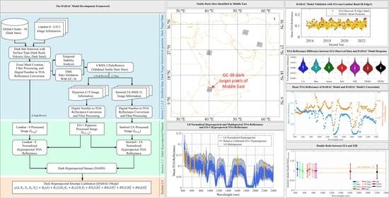
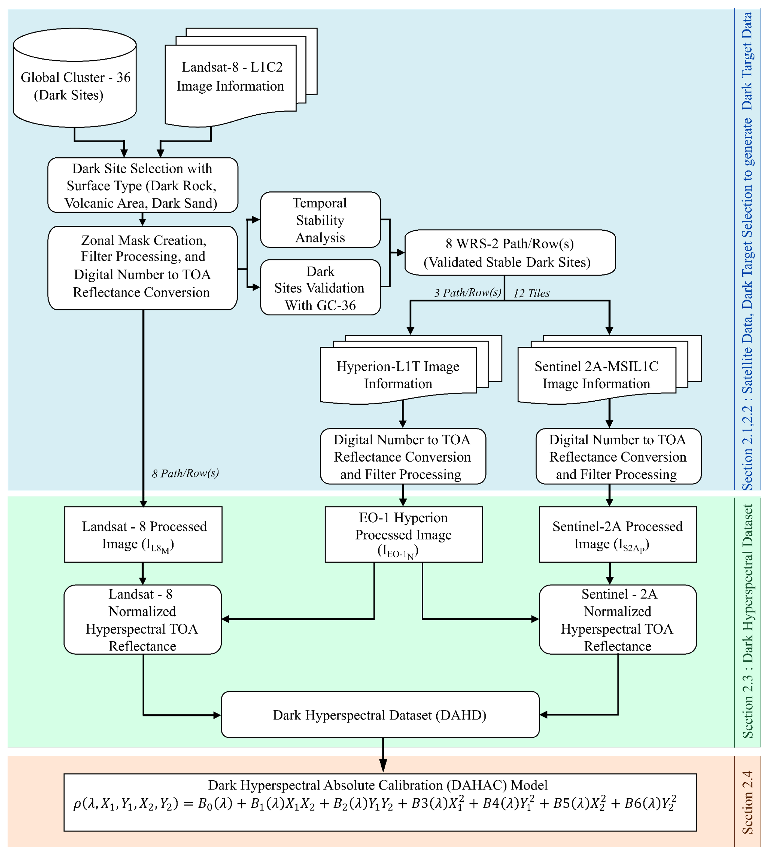
2. Methodology
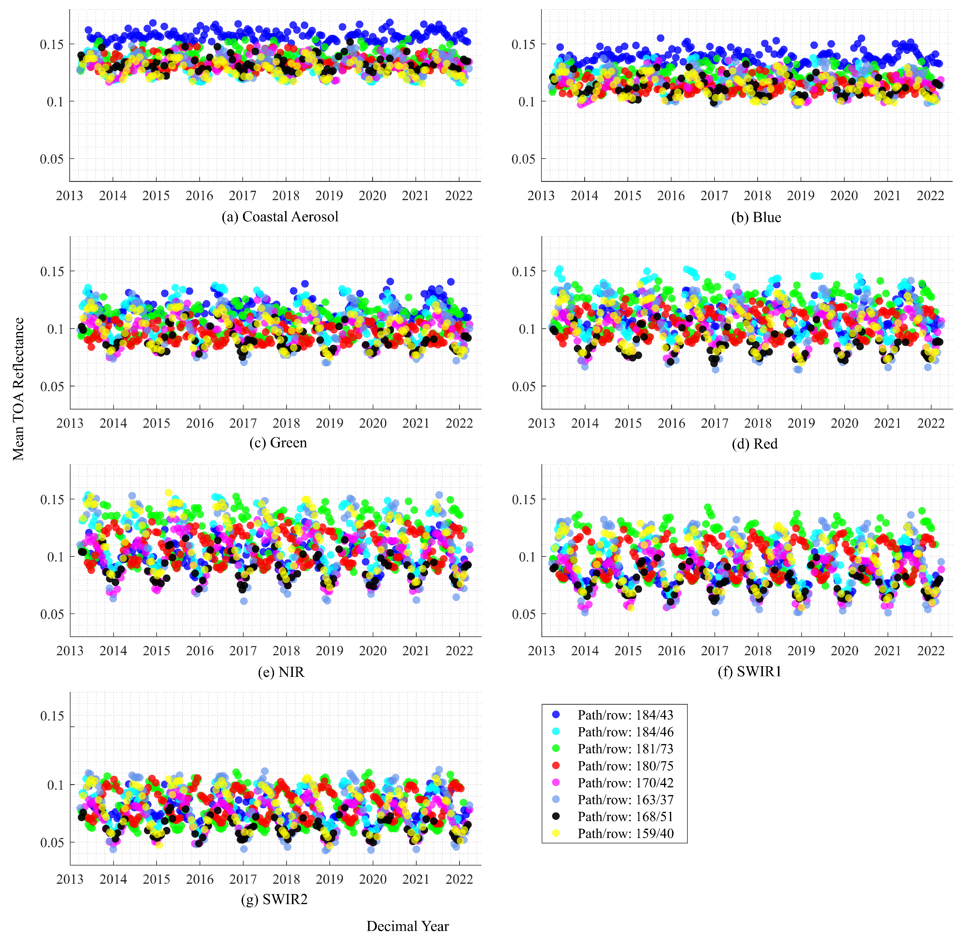
2.1. Satellite Data
2.1.1. Landsat-7, -8, -9
2.1.2. Sentinel-2A, -2B
2.1.3. Earth Observing-1 Hyperion
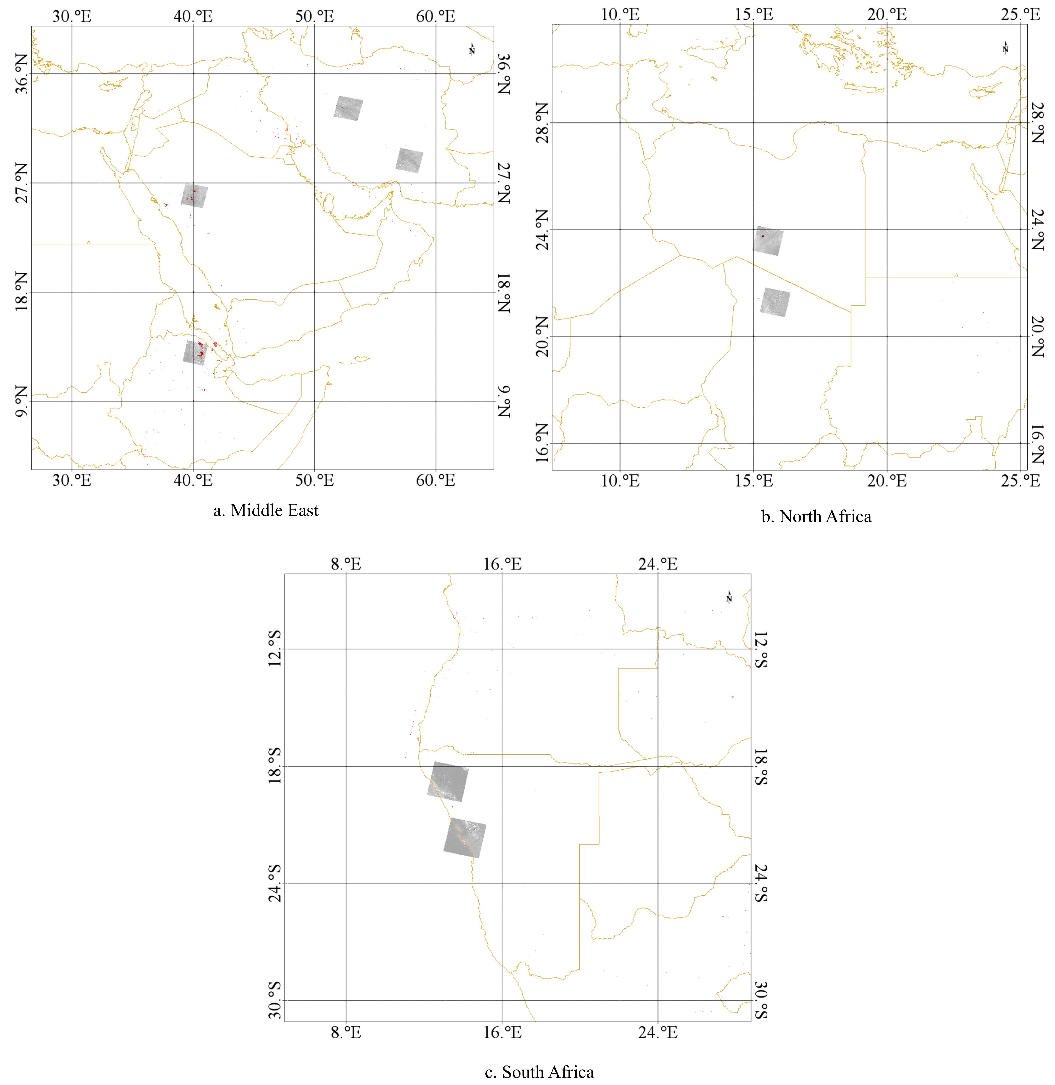
2.2. Dark Target Selection
2.2.1. Identifying Stable Dark Target Using Landsat-8
2.2.2. Creation of Zonal Mask for Satellites
2.2.3. Filtering and Dark Pixel Validation
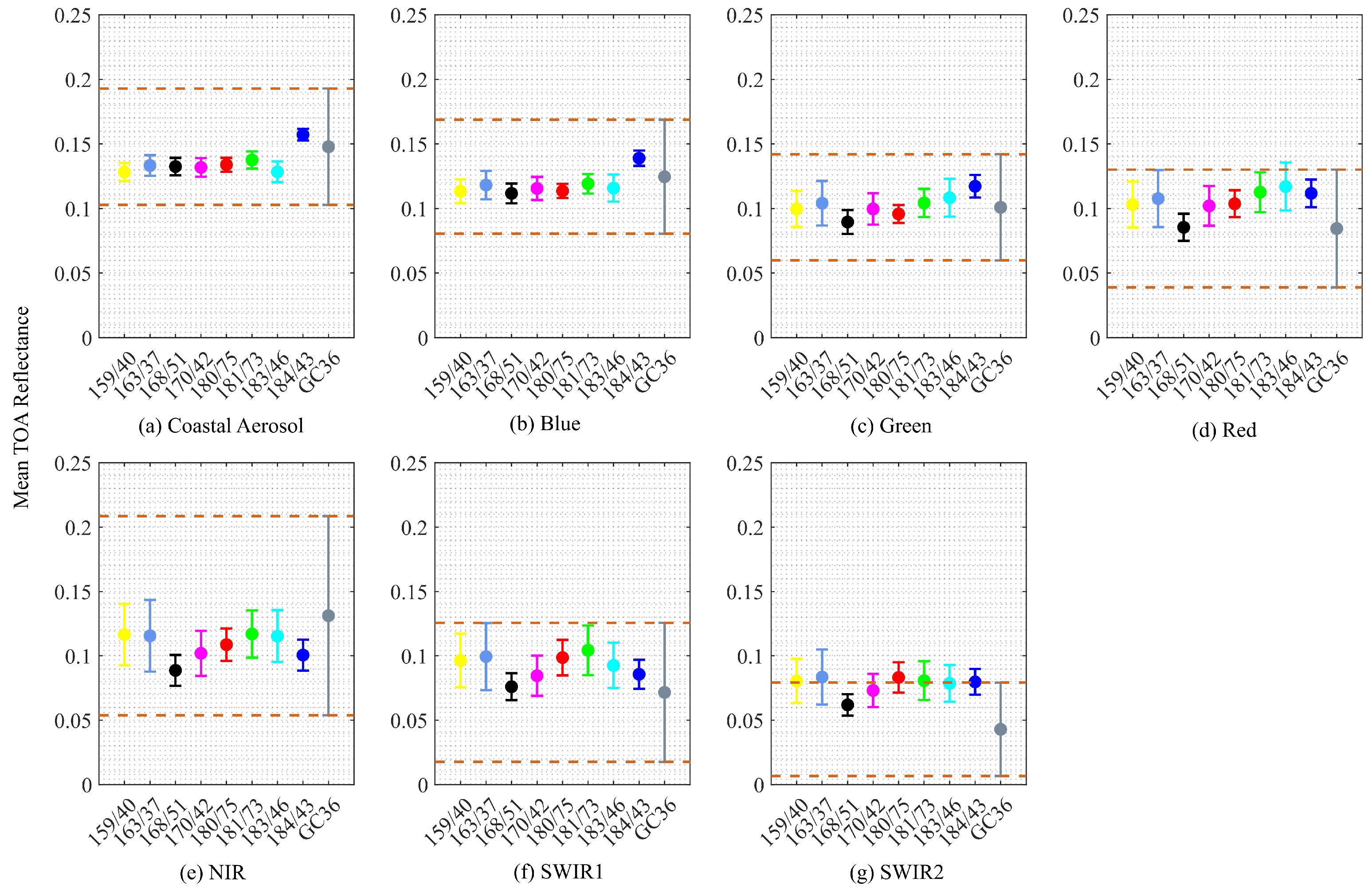
2.2.4. Dark Target Data for Absolute Calibration
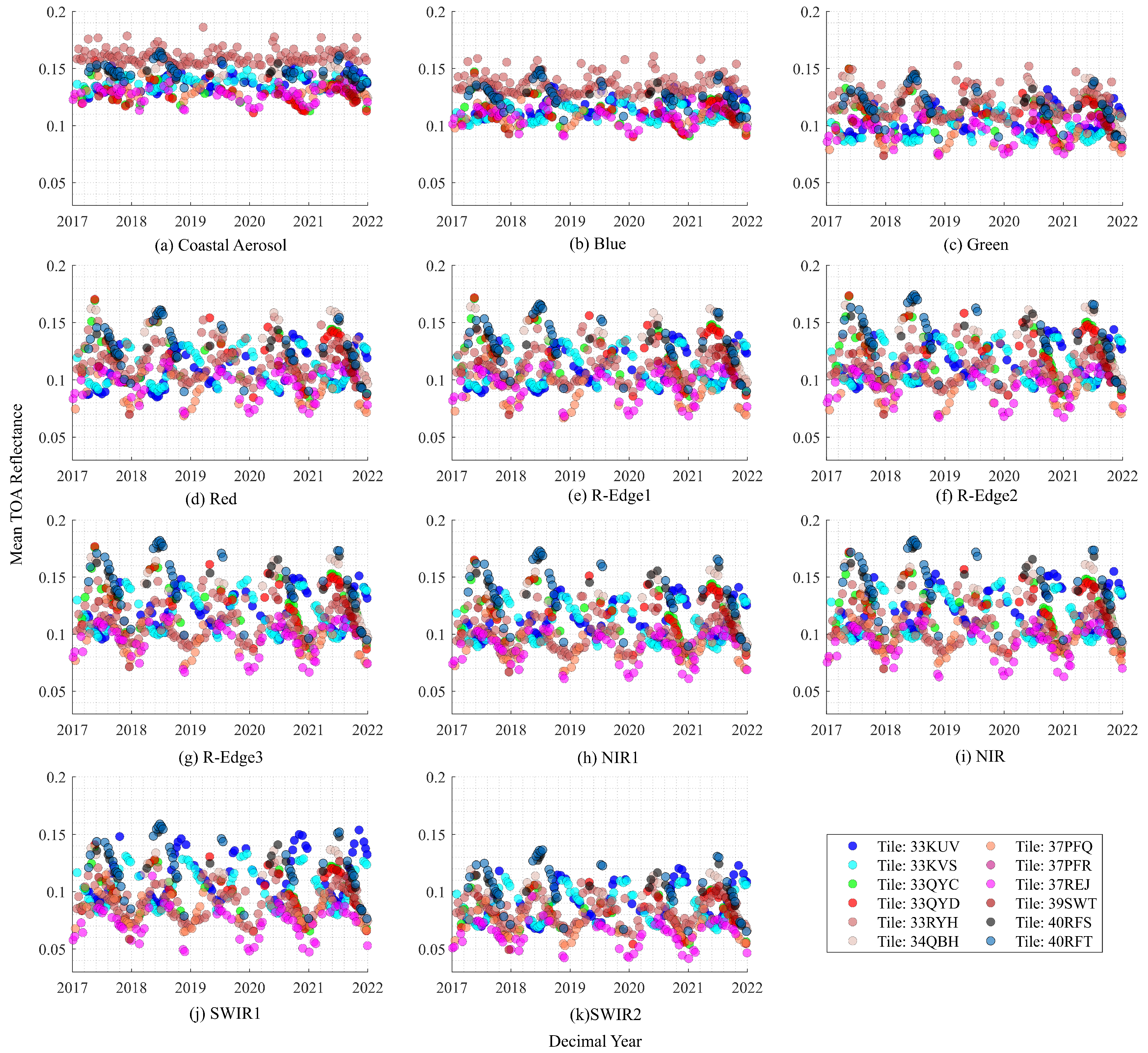
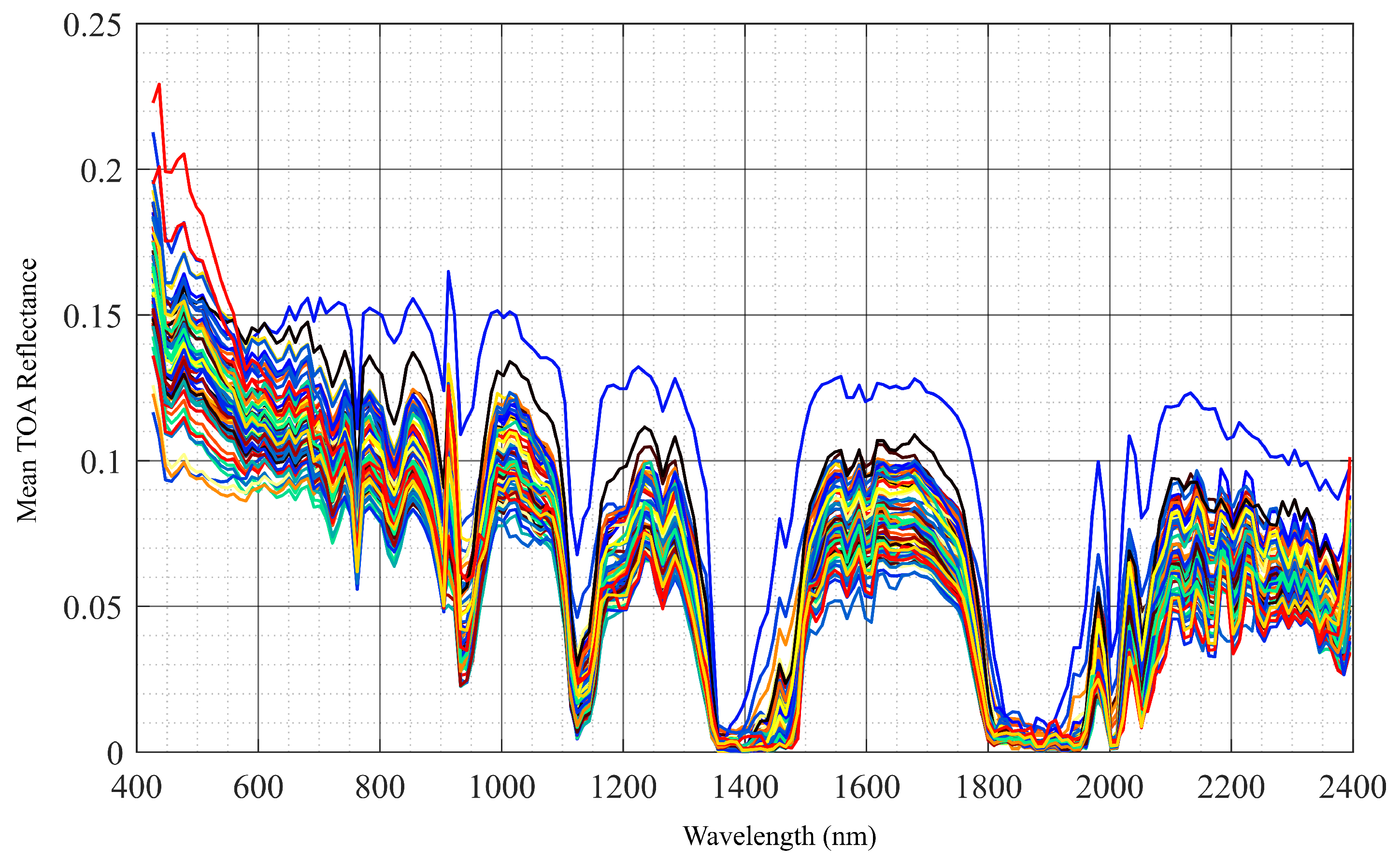
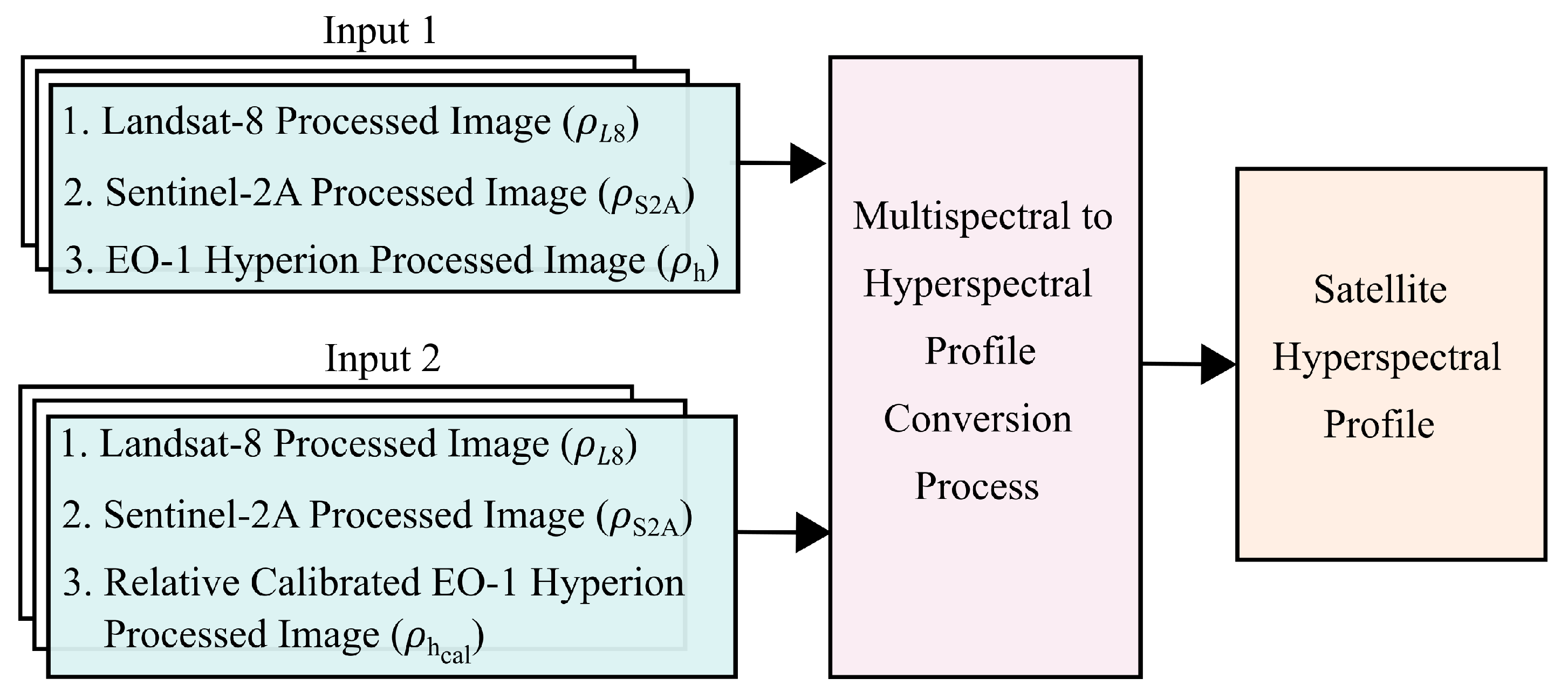
2.3. Dark Hyperspectral Dataset
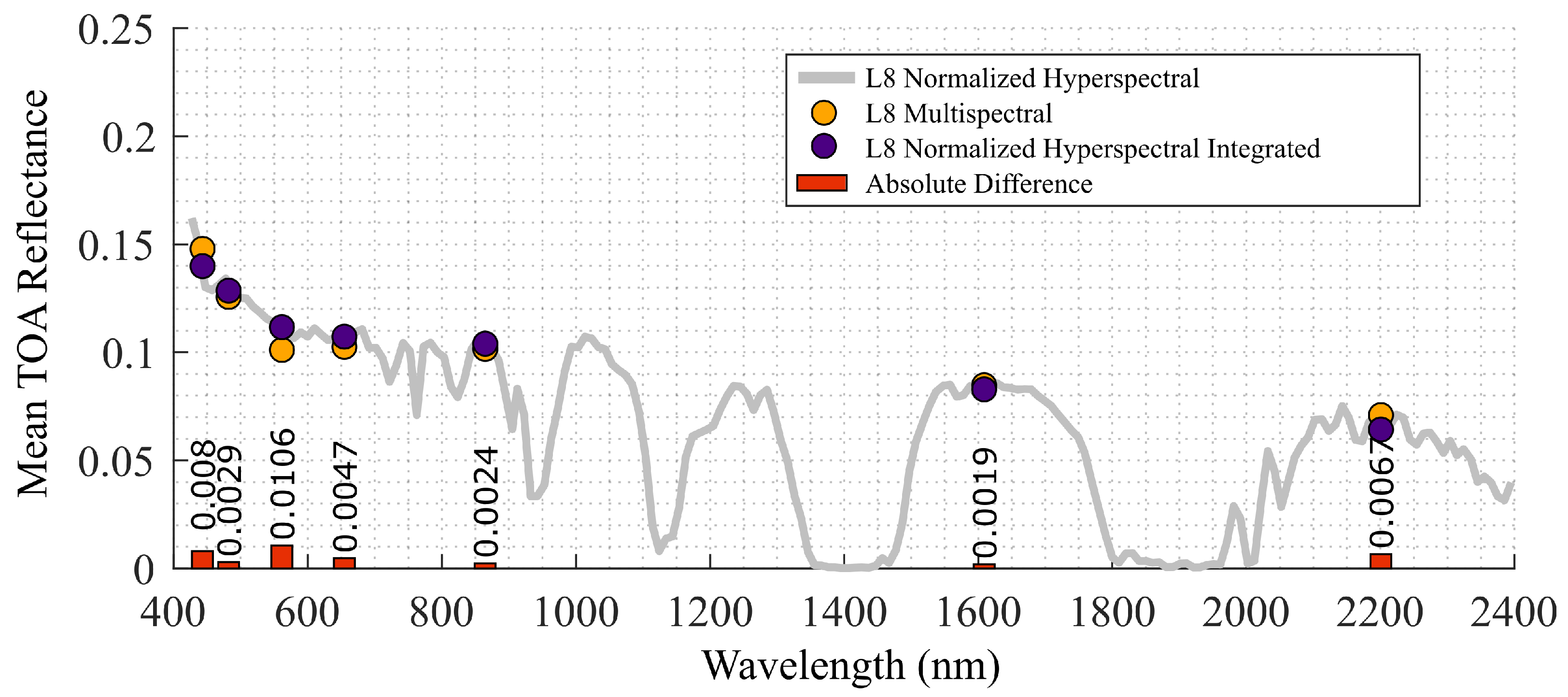
2.3.1. Estimation of Satellite Hyperspectral Profile
2.3.2. Relative Calibration on EO-1 Sensor
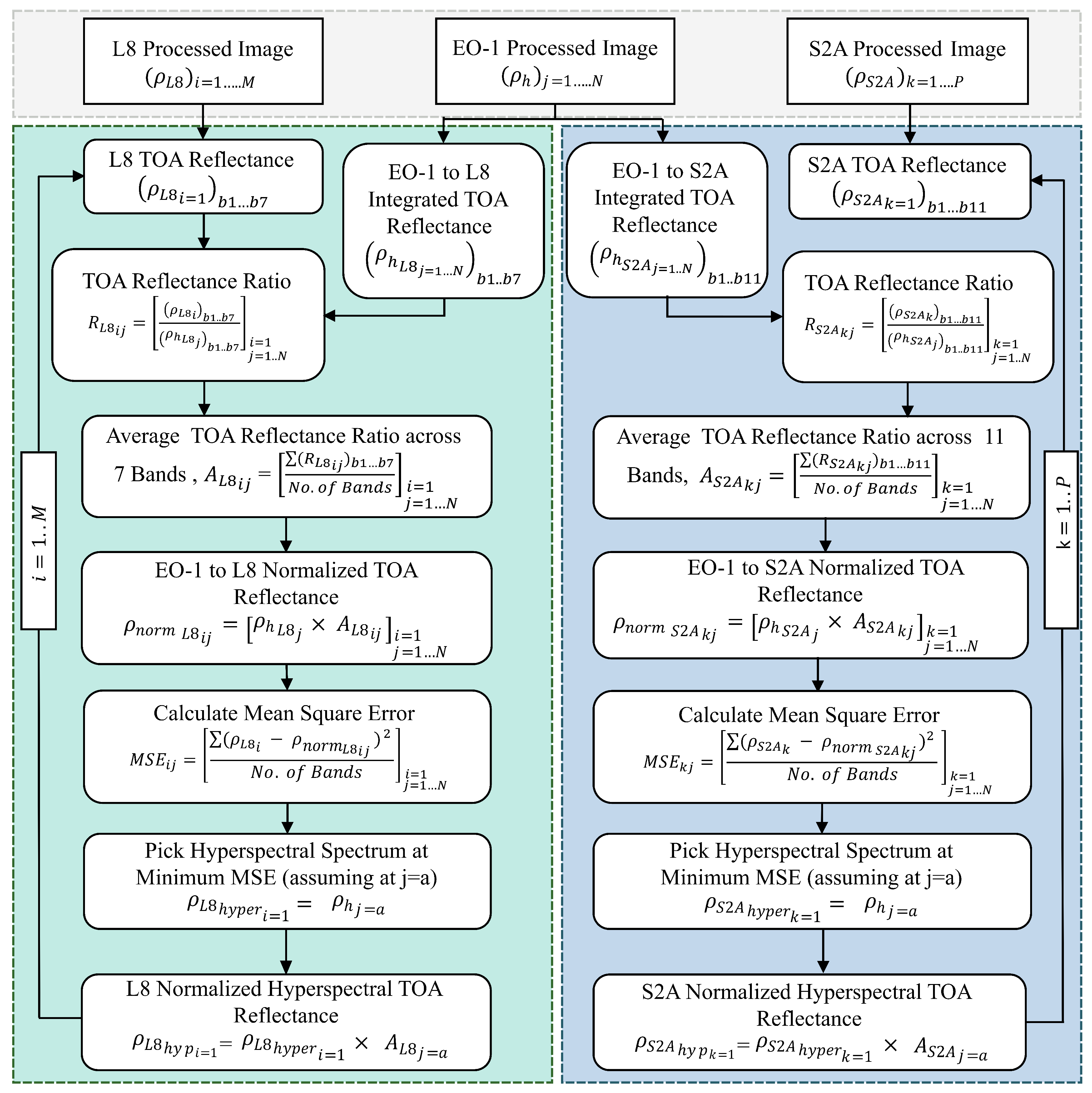
2.3.3. Normalized Hyperspectral Profile after Relative Calibration
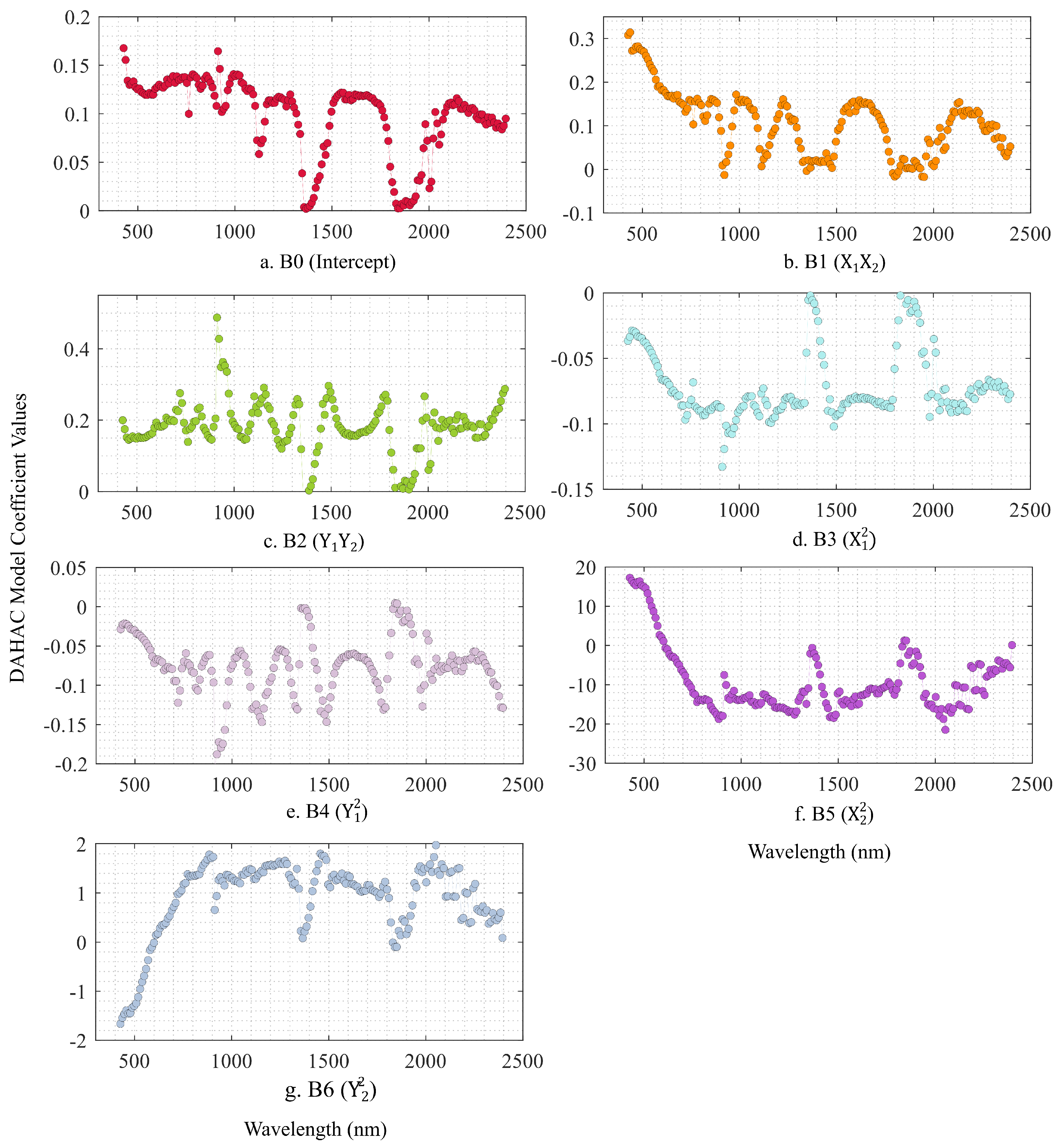
2.4. Dark Hyperspectral Absolute Calibration Model Development
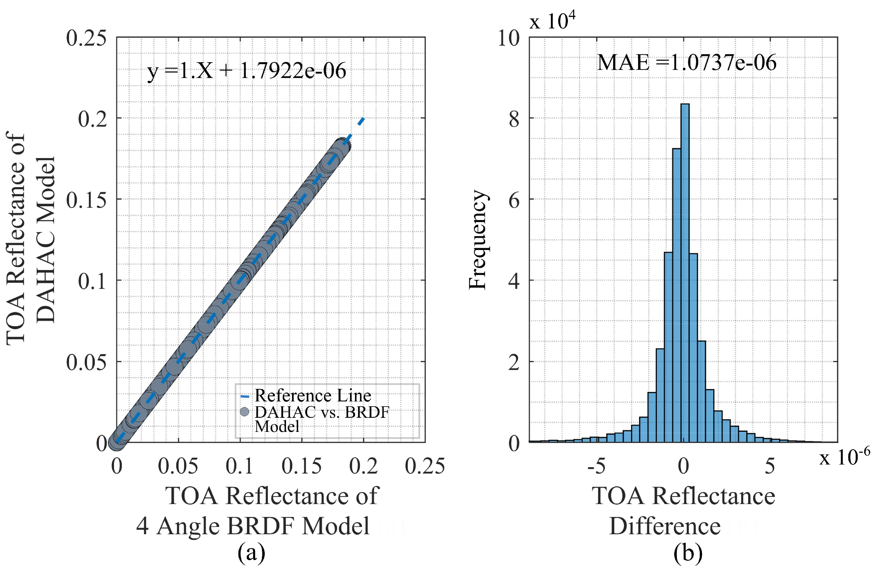
2.4.1. Four-Angle Hyperspectral BRDF Model
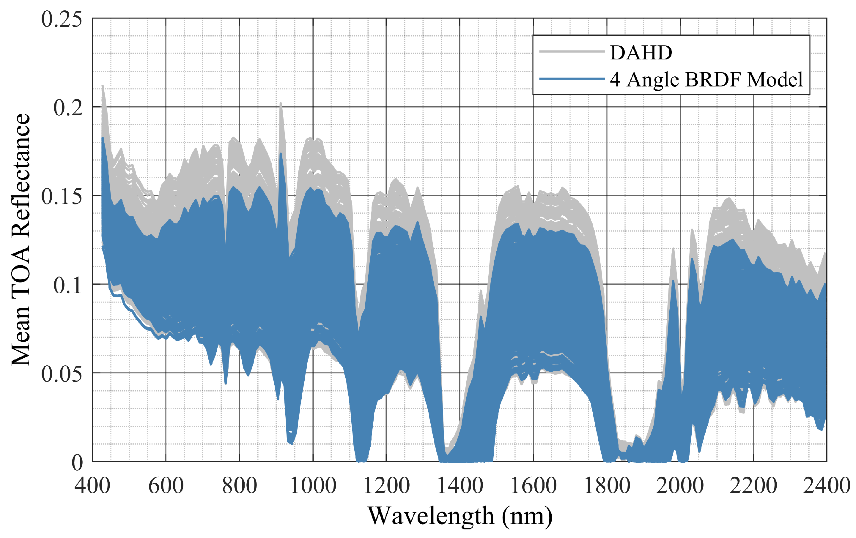
2.4.2. Dark Hyperspectral Absolute Calibration Model
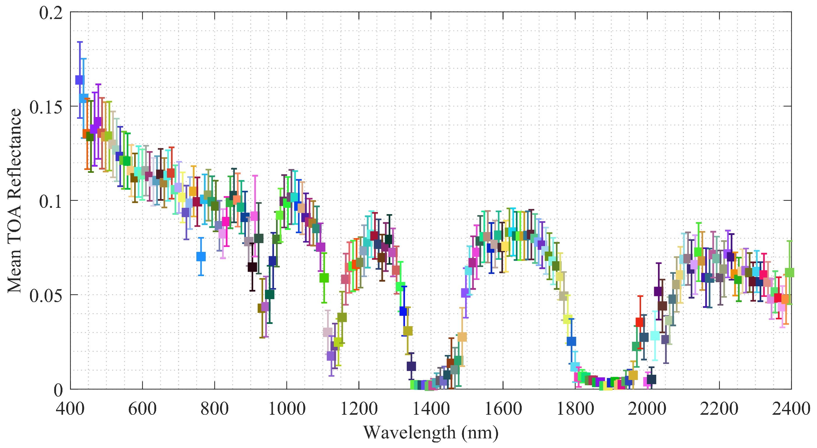
3. Results and Discussion
3.1. DAHAC Model Validation Process
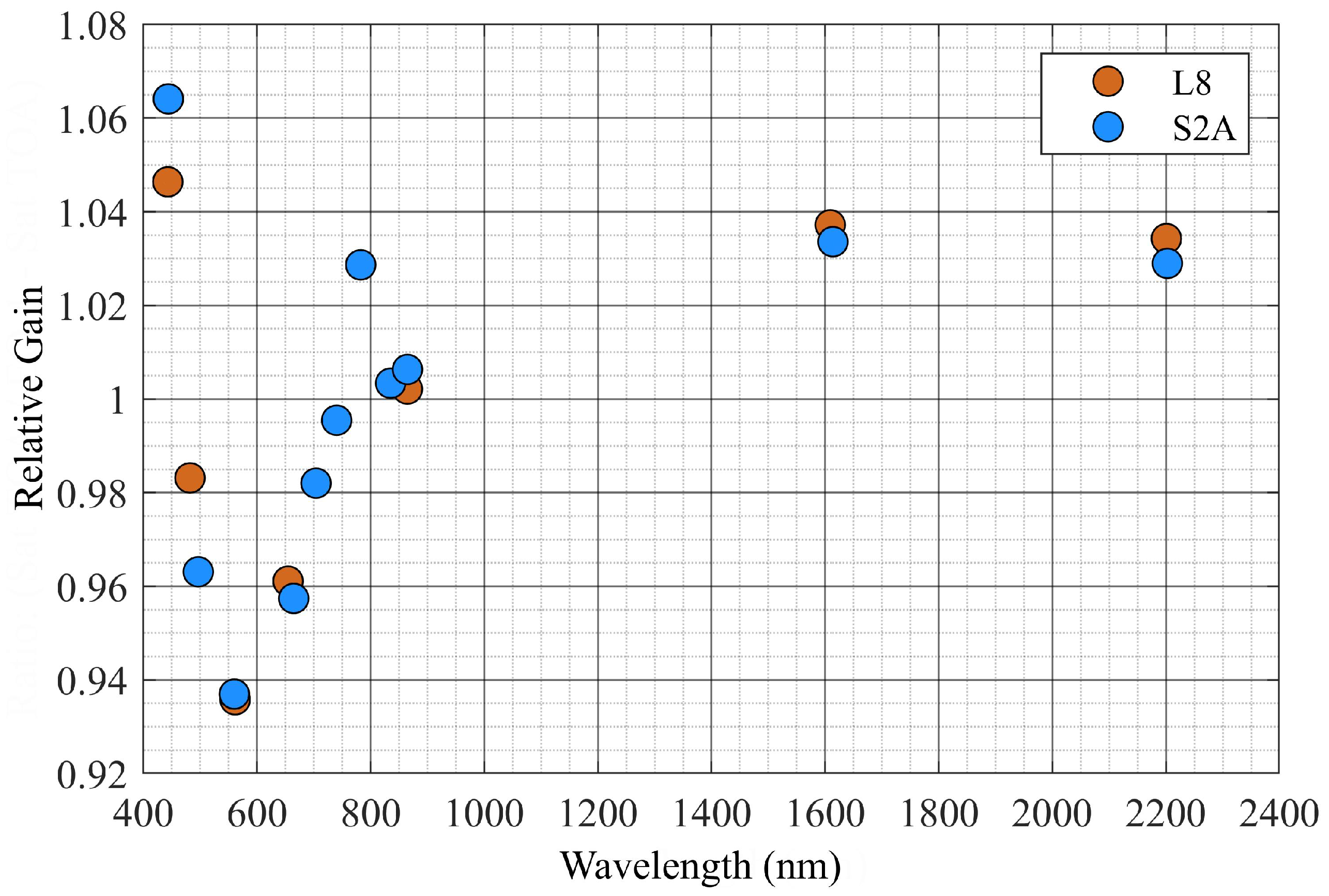
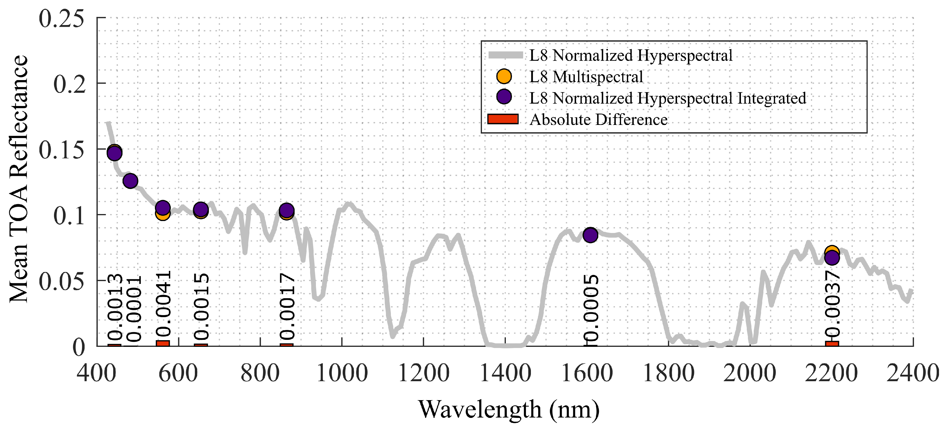
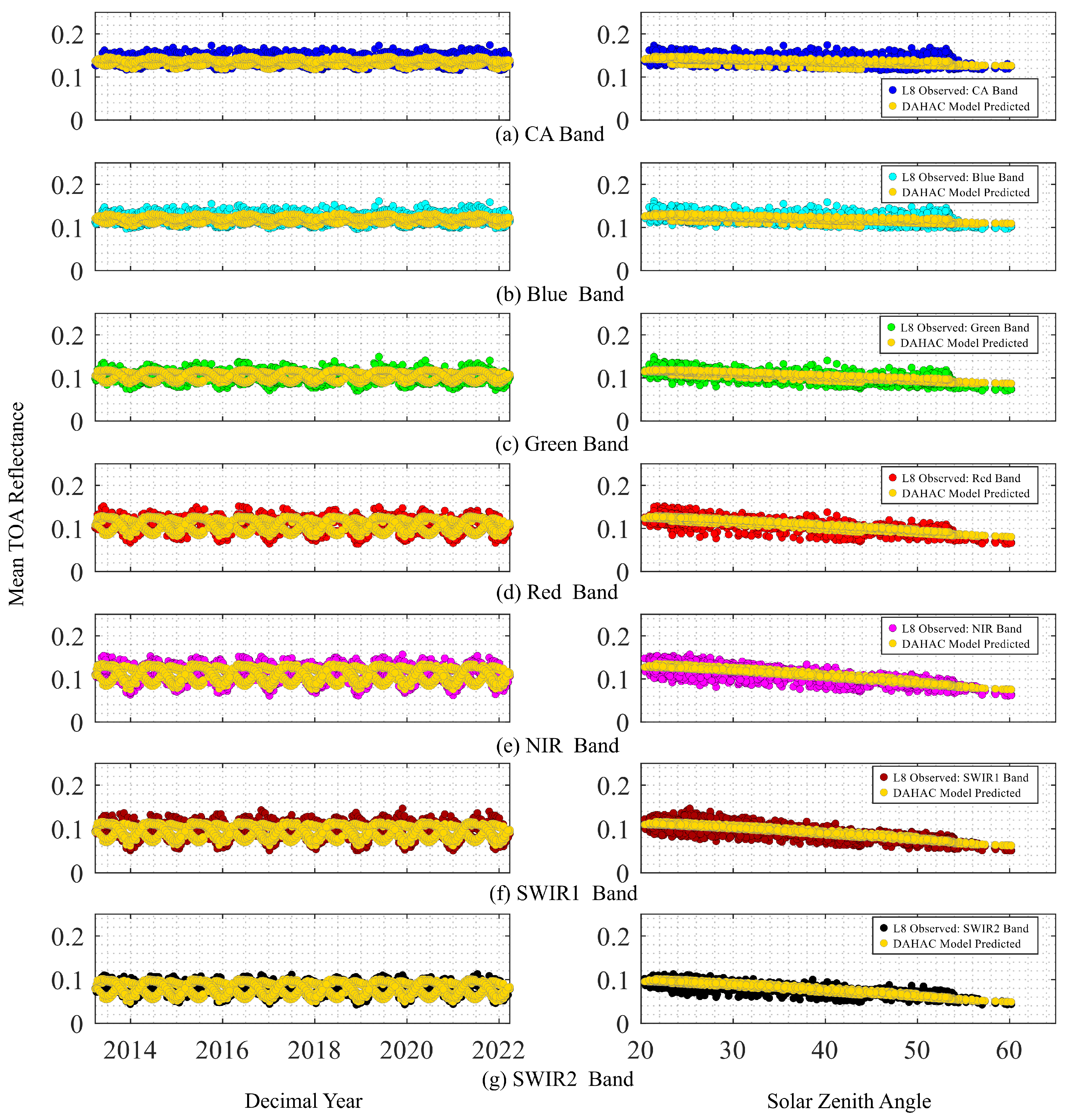
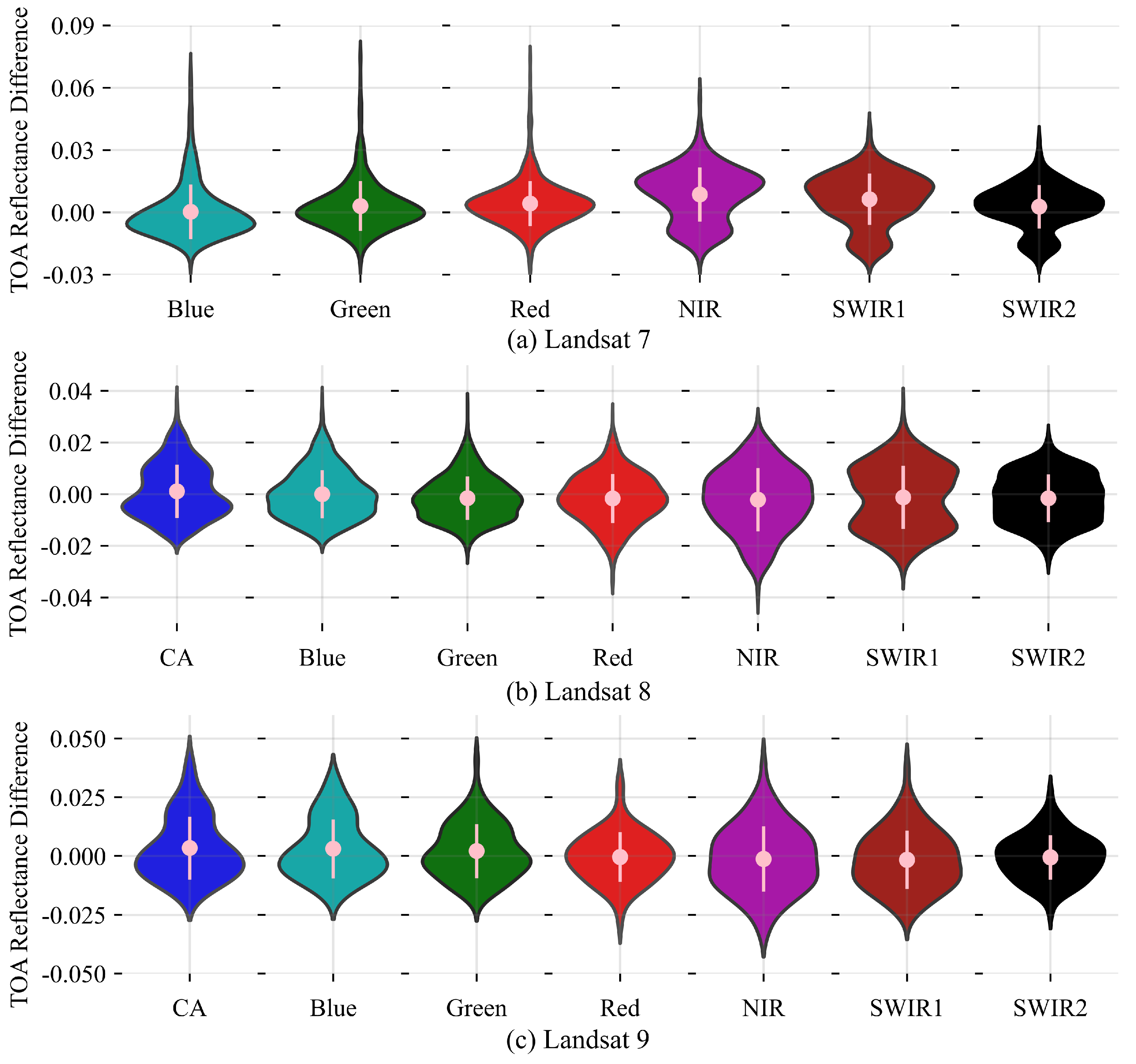
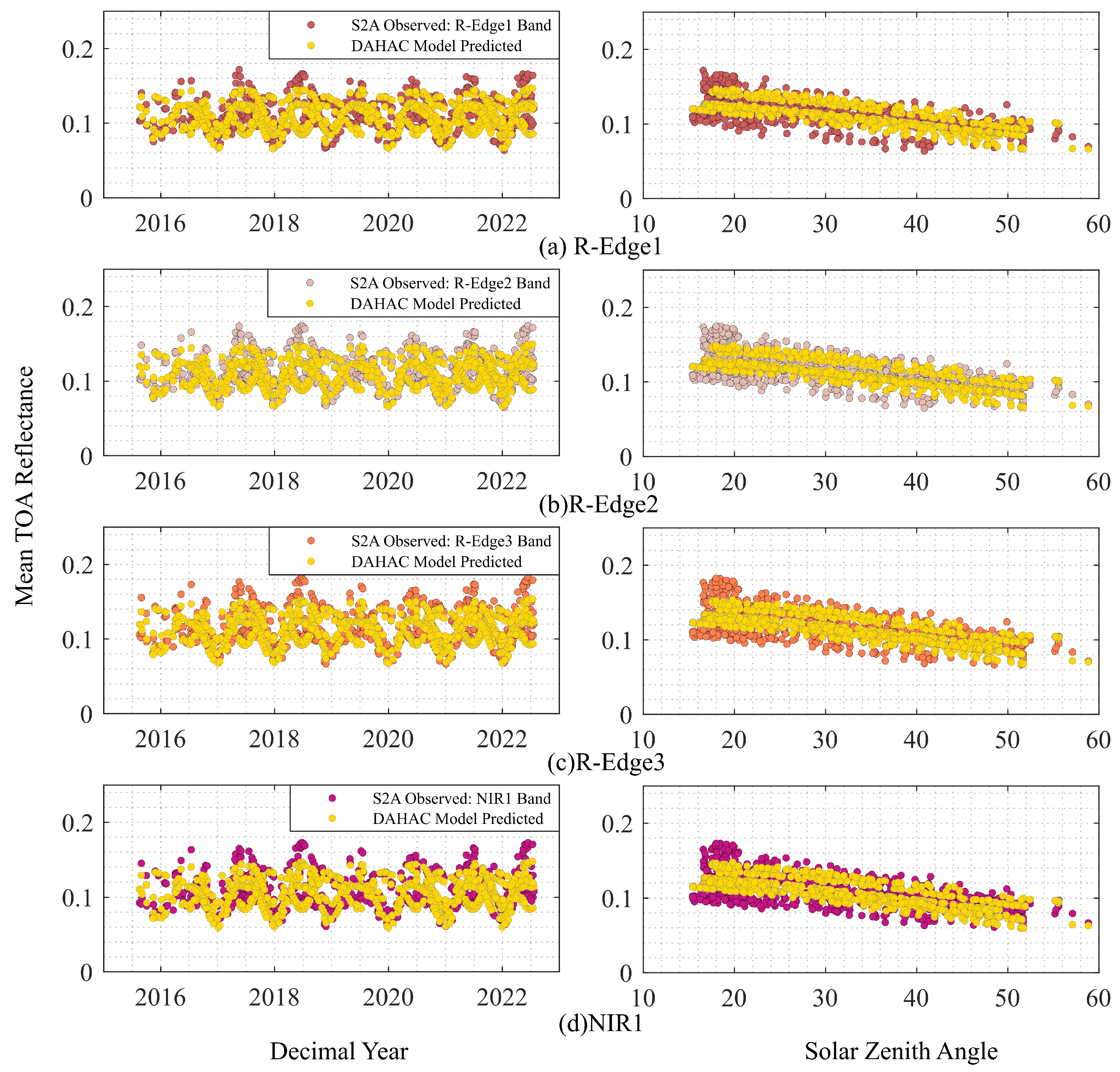
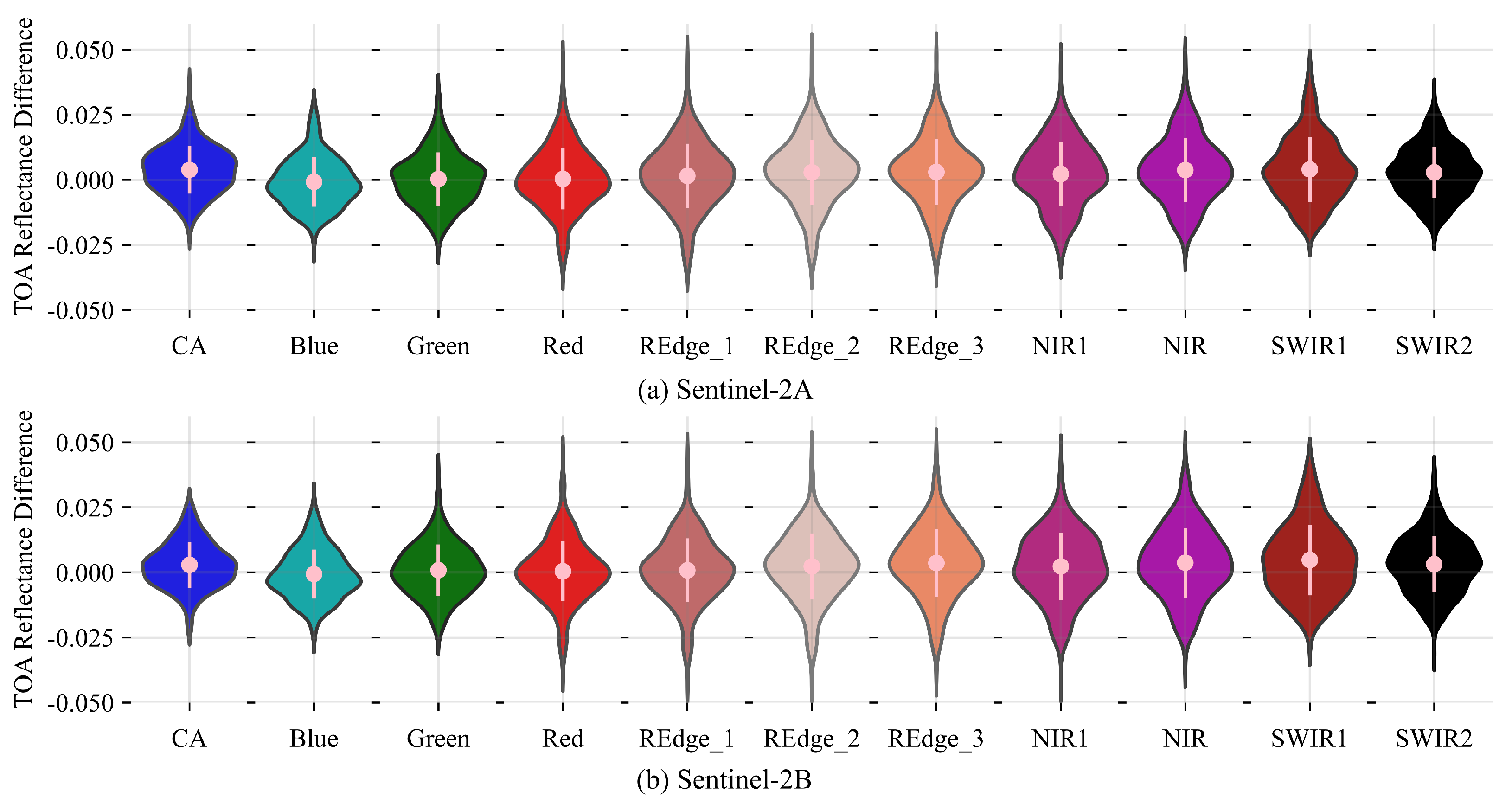
3.1.1. DAHAC Model Validation with Landsat Missions
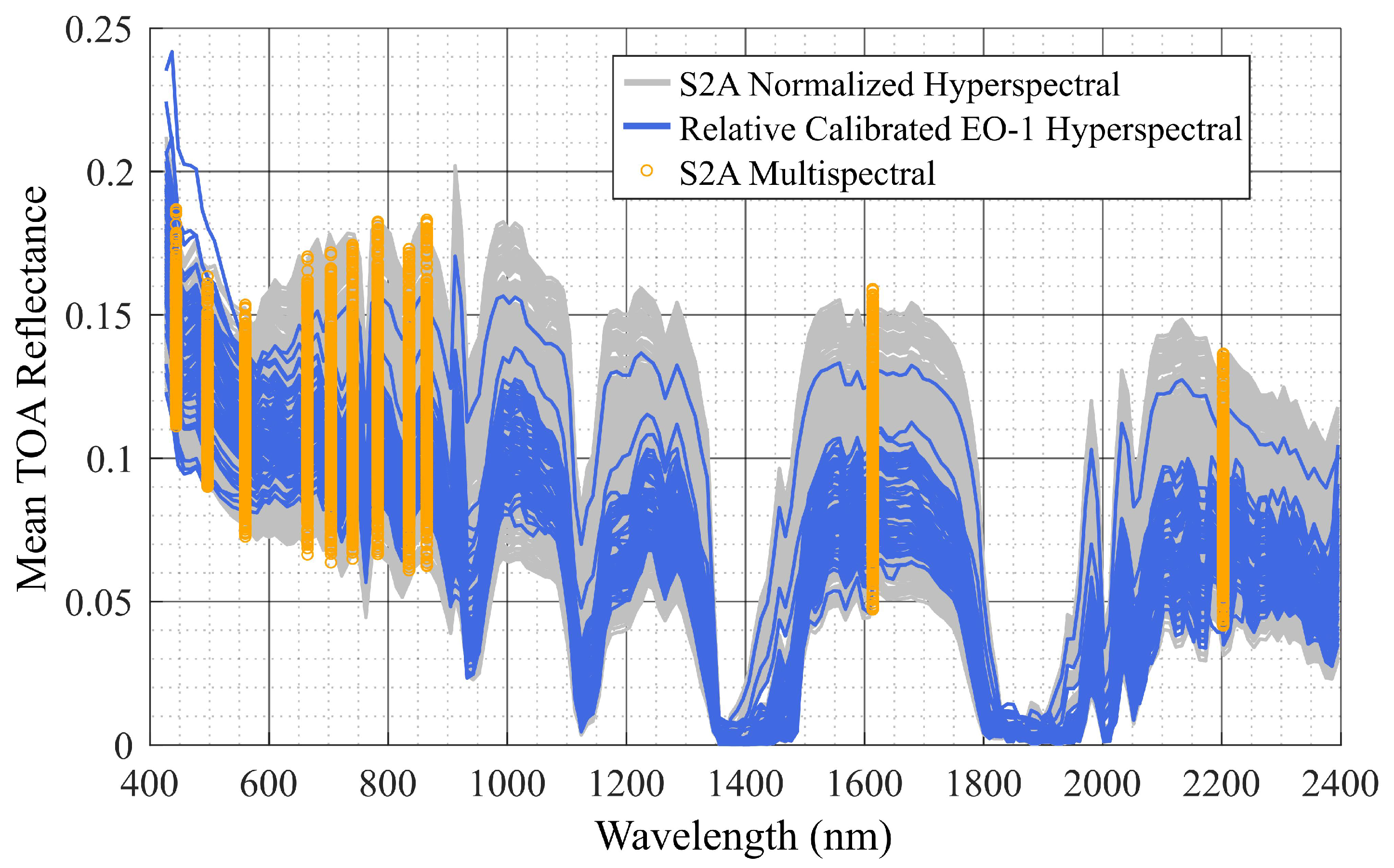
3.1.2. DAHAC Model Validation with Sentinel-2 Missions
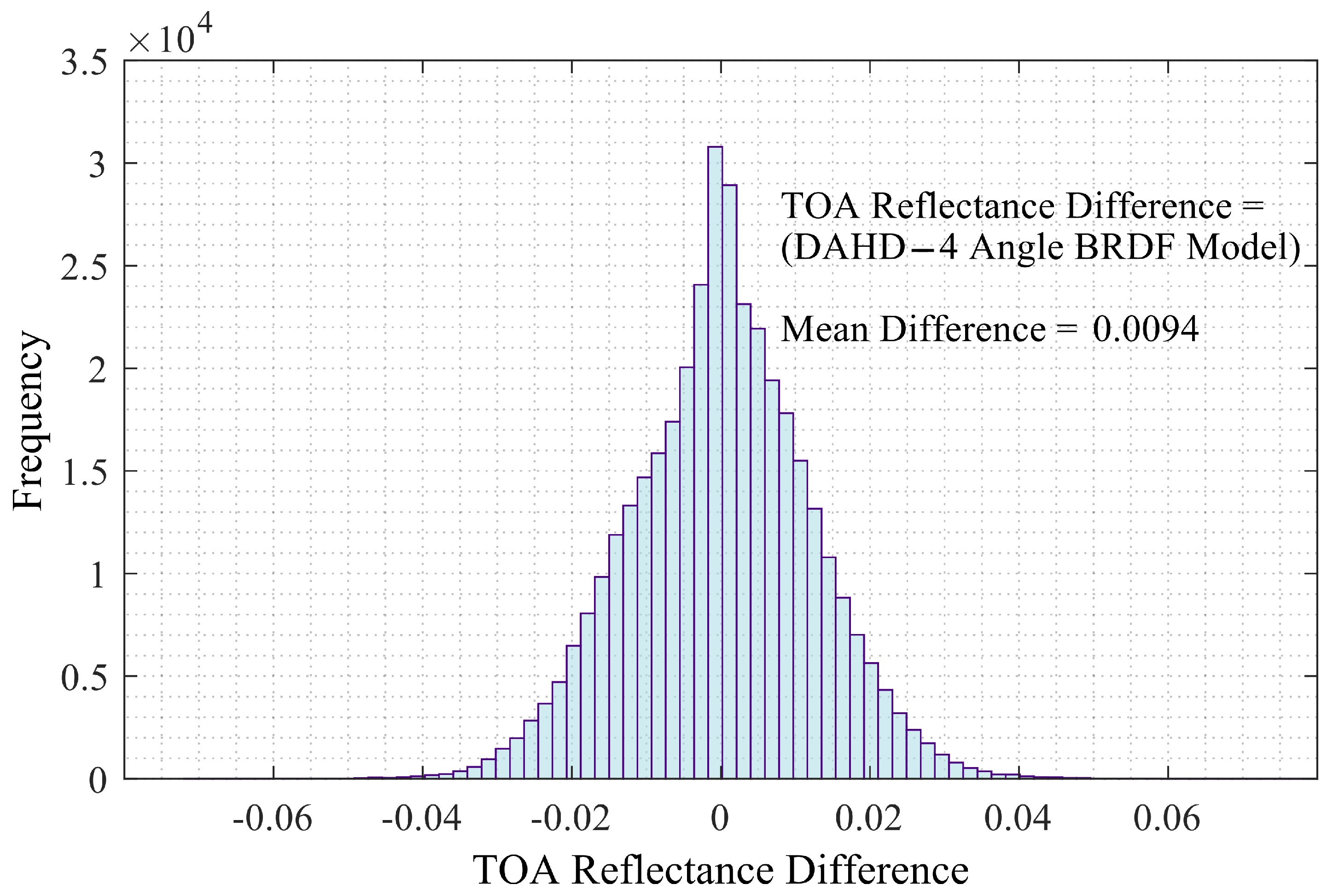
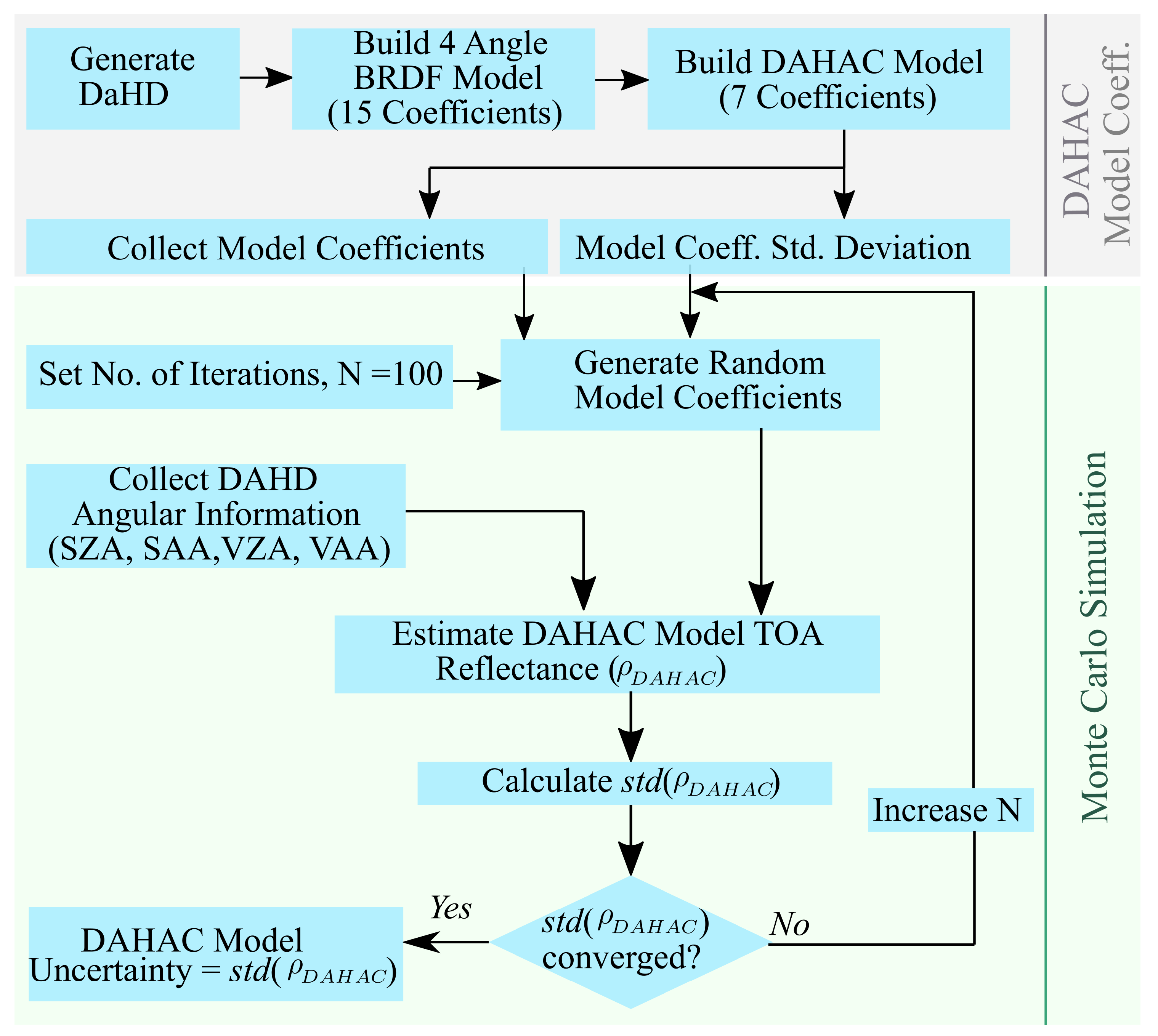
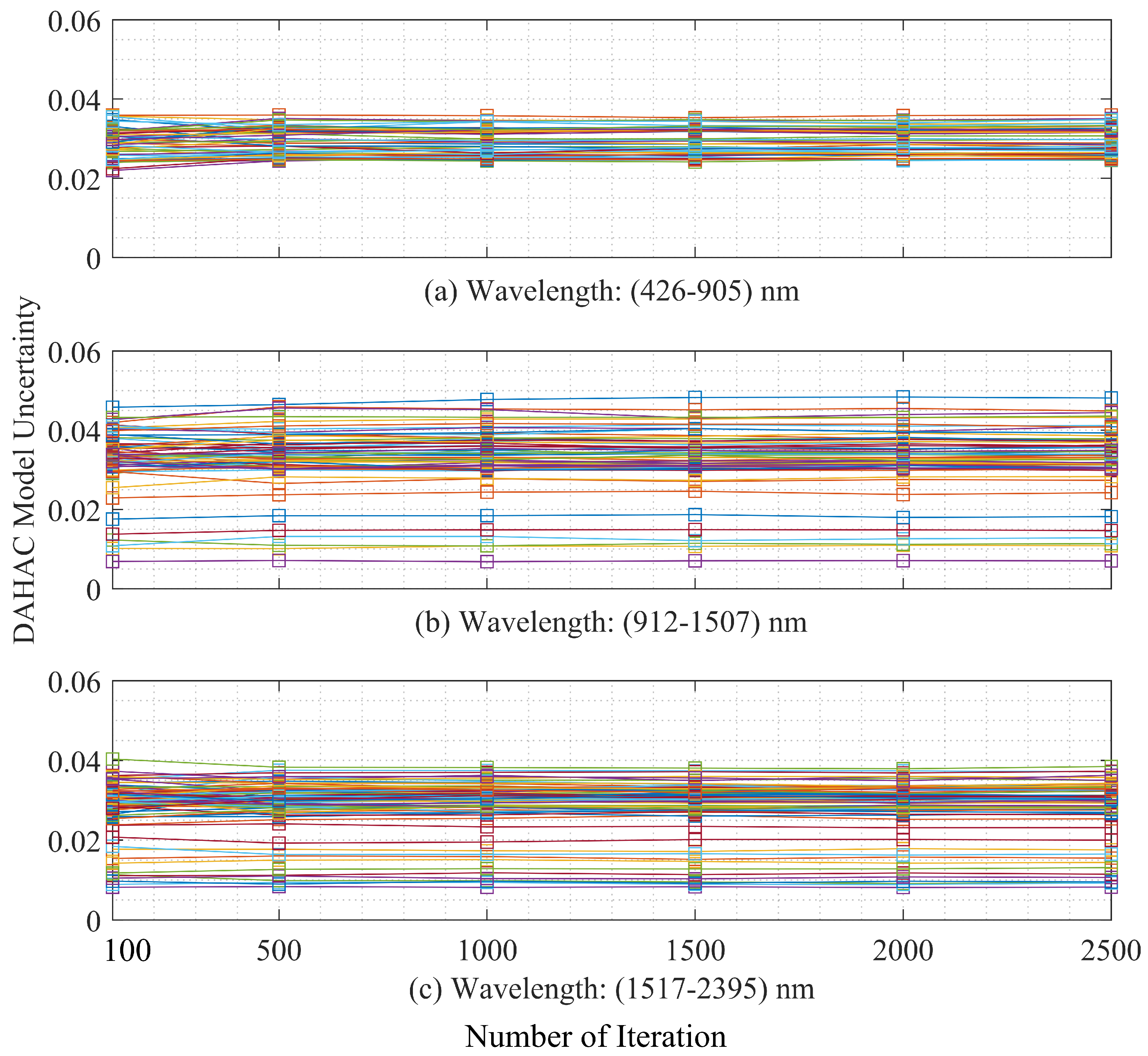
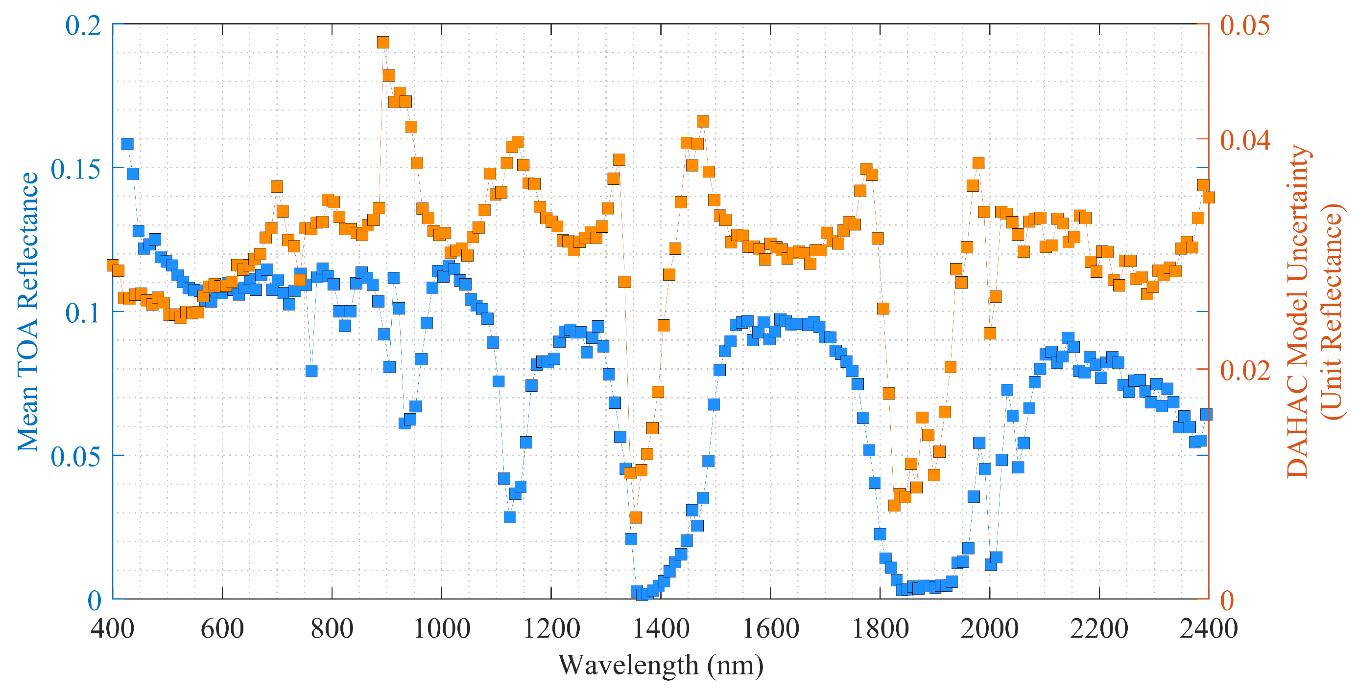
4. Uncertainty Analysis
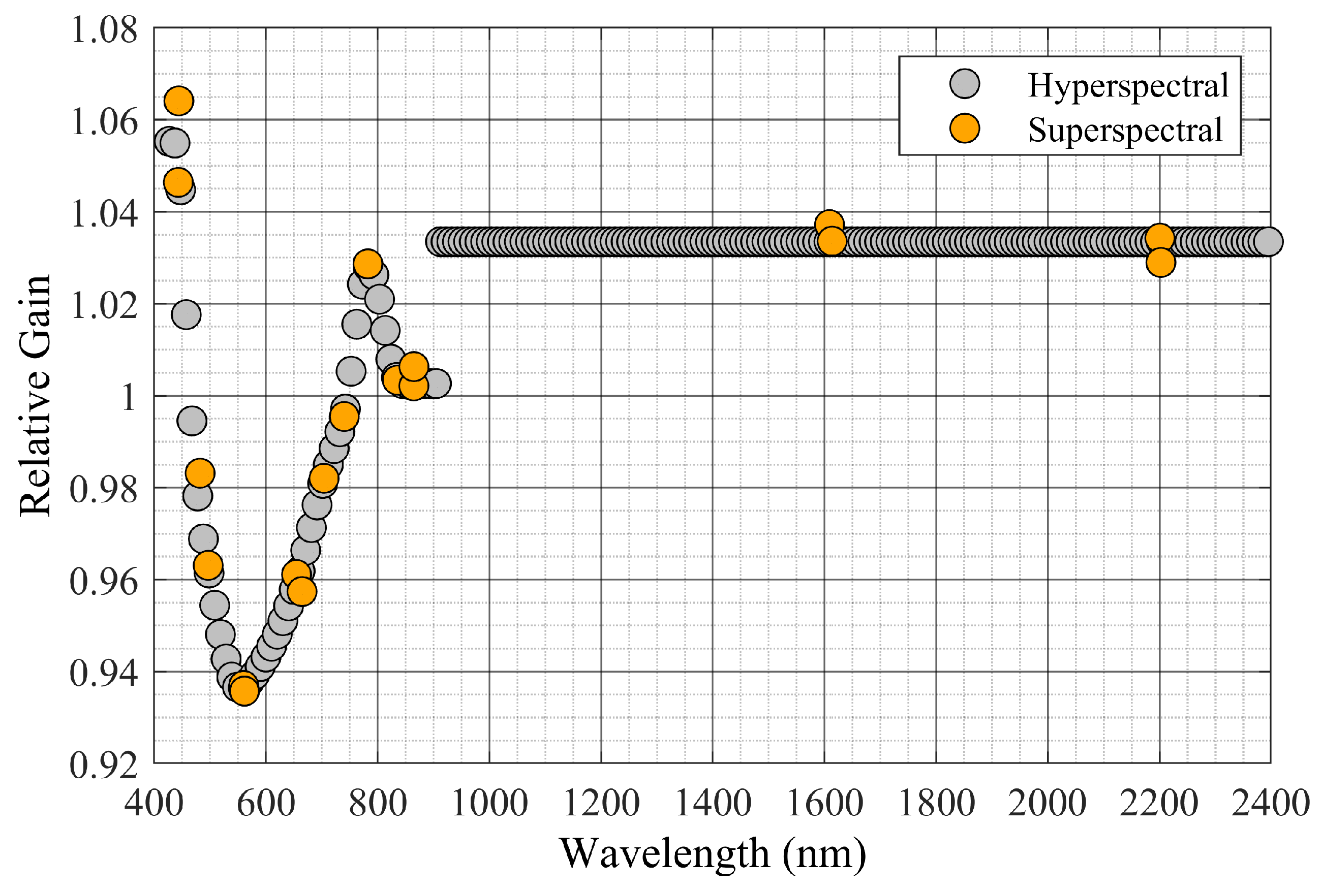
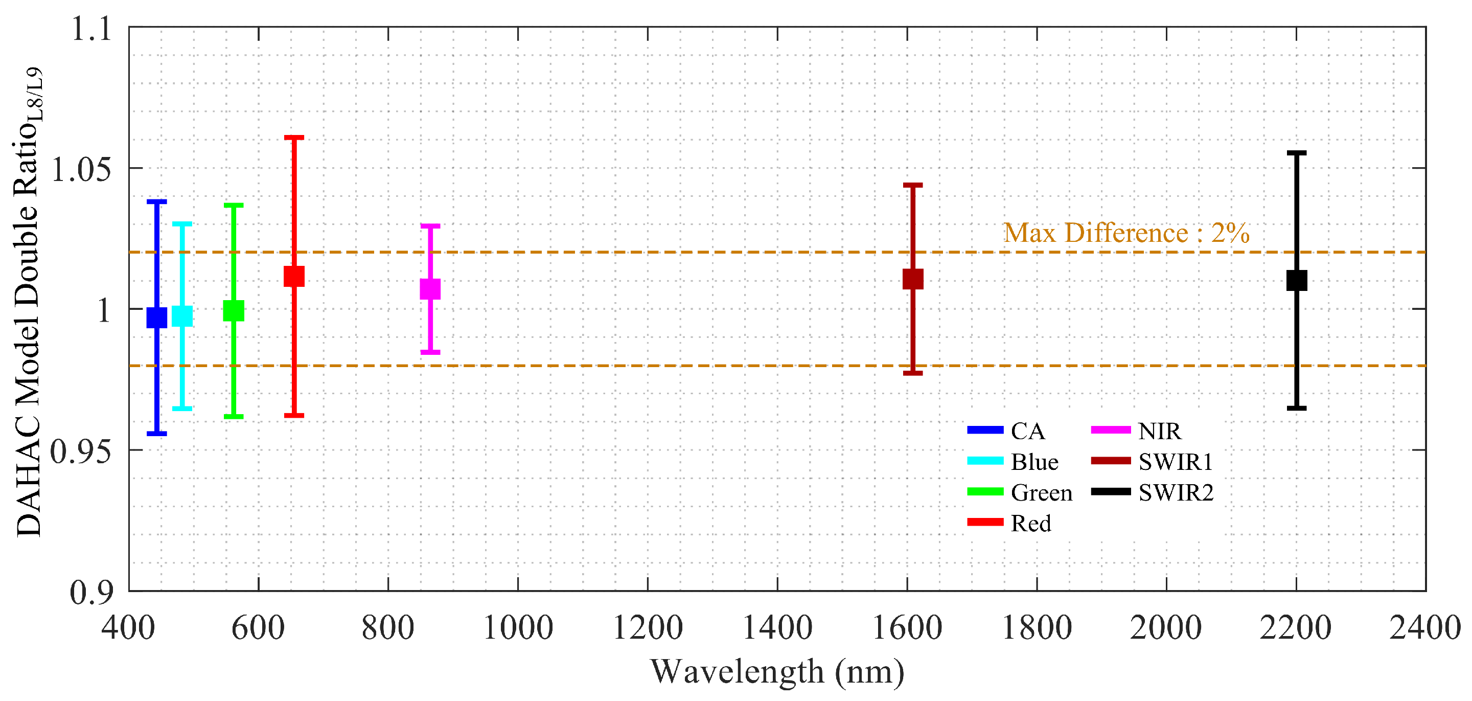
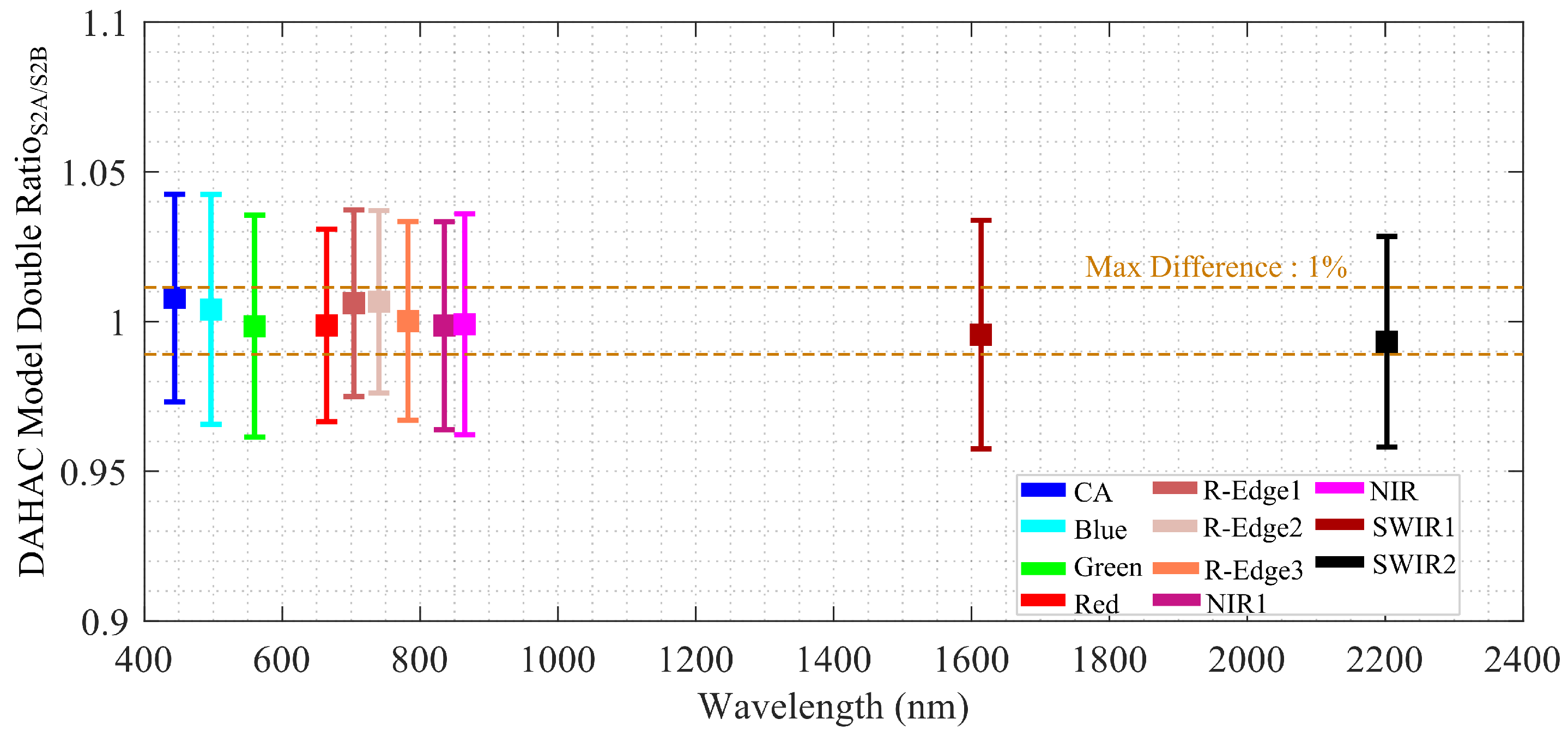
5. The DAHAC Model’s Double Ratio for Sensors Inter-Comparison
6. Conclusions
Author Contributions
Funding
Data Availability Statement
Acknowledgments
Conflicts of Interest
Appendix A

| Wavelength (nm) | ||||||||||||||
|---|---|---|---|---|---|---|---|---|---|---|---|---|---|---|
| 426.8 | 0.168 | 5.90E-04 | 0.308 | 1.70E-02 | 0.2 | 6.90E-03 | −0.037 | 8.00E-04 | −0.029 | 3.20E-03 | 17.243 | 4.70E-01 | −1.666 | 4.30E-02 |
| 437 | 0.155 | 5.50E-04 | 0.314 | 1.60E-02 | 0.175 | 6.40E-03 | −0.034 | 7.40E-04 | −0.023 | 3.00E-03 | 16.453 | 4.40E-01 | −1.542 | 4.00E-02 |
| 447.2 | 0.134 | 4.90E-04 | 0.272 | 1.40E-02 | 0.152 | 5.70E-03 | −0.029 | 6.60E-04 | −0.021 | 2.70E-03 | 15.8 | 3.90E-01 | −1.463 | 3.60E-02 |
| 457.3 | 0.13 | 4.70E-04 | 0.274 | 1.40E-02 | 0.145 | 5.50E-03 | −0.029 | 6.40E-04 | −0.022 | 2.60E-03 | 15.326 | 3.80E-01 | −1.391 | 3.50E-02 |
| 467.5 | 0.131 | 4.80E-04 | 0.281 | 1.40E-02 | 0.149 | 5.60E-03 | −0.03 | 6.50E-04 | −0.025 | 2.60E-03 | 16.189 | 3.90E-01 | −1.455 | 3.50E-02 |
| 477.7 | 0.133 | 4.90E-04 | 0.282 | 1.40E-02 | 0.155 | 5.70E-03 | −0.033 | 6.60E-04 | −0.028 | 2.70E-03 | 16.335 | 3.90E-01 | −1.449 | 3.60E-02 |
| 487.9 | 0.127 | 4.60E-04 | 0.275 | 1.30E-02 | 0.149 | 5.40E-03 | −0.034 | 6.20E-04 | −0.029 | 2.50E-03 | 15.26 | 3.70E-01 | −1.335 | 3.40E-02 |
| 498 | 0.125 | 4.60E-04 | 0.272 | 1.30E-02 | 0.148 | 5.30E-03 | −0.035 | 6.20E-04 | −0.03 | 2.50E-03 | 14.998 | 3.60E-01 | −1.299 | 3.40E-02 |
| 508.2 | 0.126 | 4.50E-04 | 0.27 | 1.30E-02 | 0.154 | 5.30E-03 | −0.037 | 6.10E-04 | −0.034 | 2.50E-03 | 14.561 | 3.60E-01 | −1.247 | 3.40E-02 |
| 518.4 | 0.122 | 4.40E-04 | 0.26 | 1.30E-02 | 0.15 | 5.10E-03 | −0.038 | 5.90E-04 | −0.035 | 2.40E-03 | 13.24 | 3.50E-01 | −1.12 | 3.20E-02 |
| 528.6 | 0.121 | 4.20E-04 | 0.252 | 1.20E-02 | 0.15 | 4.90E-03 | −0.041 | 5.70E-04 | −0.037 | 2.30E-03 | 11.479 | 3.40E-01 | −0.953 | 3.10E-02 |
| 538.7 | 0.12 | 4.10E-04 | 0.241 | 1.20E-02 | 0.151 | 4.80E-03 | −0.043 | 5.50E-04 | −0.04 | 2.20E-03 | 9.941 | 3.30E-01 | −0.812 | 3.00E-02 |
| 548.9 | 0.119 | 4.00E-04 | 0.232 | 1.20E-02 | 0.153 | 4.70E-03 | −0.046 | 5.50E-04 | −0.043 | 2.20E-03 | 8.645 | 3.20E-01 | −0.69 | 3.00E-02 |
| 559.1 | 0.121 | 4.10E-04 | 0.225 | 1.20E-02 | 0.158 | 4.80E-03 | −0.049 | 5.50E-04 | −0.046 | 2.20E-03 | 7.054 | 3.30E-01 | −0.546 | 3.00E-02 |
| 569.3 | 0.12 | 4.00E-04 | 0.206 | 1.20E-02 | 0.16 | 4.70E-03 | −0.052 | 5.40E-04 | −0.051 | 2.20E-03 | 5.003 | 3.20E-01 | −0.367 | 2.90E-02 |
| 579.5 | 0.12 | 4.00E-04 | 0.189 | 1.20E-02 | 0.164 | 4.70E-03 | −0.056 | 5.40E-04 | −0.055 | 2.20E-03 | 2.653 | 3.20E-01 | −0.161 | 3.00E-02 |
| 589.6 | 0.126 | 4.30E-04 | 0.191 | 1.30E-02 | 0.179 | 5.10E-03 | −0.062 | 5.90E-04 | −0.063 | 2.40E-03 | 2.091 | 3.50E-01 | −0.103 | 3.20E-02 |
| 599.8 | 0.128 | 4.60E-04 | 0.181 | 1.30E-02 | 0.193 | 5.40E-03 | −0.066 | 6.20E-04 | −0.072 | 2.50E-03 | 1.091 | 3.70E-01 | −0.012 | 3.40E-02 |
| 610 | 0.13 | 4.60E-04 | 0.182 | 1.30E-02 | 0.183 | 5.30E-03 | −0.067 | 6.20E-04 | −0.067 | 2.50E-03 | −0.664 | 3.70E-01 | 0.144 | 3.40E-02 |
| 620.1 | 0.128 | 4.50E-04 | 0.175 | 1.30E-02 | 0.181 | 5.30E-03 | −0.067 | 6.10E-04 | −0.067 | 2.50E-03 | −1.025 | 3.60E-01 | 0.175 | 3.30E-02 |
| 630.3 | 0.127 | 4.60E-04 | 0.168 | 1.30E-02 | 0.182 | 5.40E-03 | −0.068 | 6.20E-04 | −0.069 | 2.50E-03 | −2.241 | 3.70E-01 | 0.284 | 3.40E-02 |
| 640.5 | 0.129 | 4.70E-04 | 0.168 | 1.40E-02 | 0.186 | 5.50E-03 | −0.07 | 6.40E-04 | −0.071 | 2.60E-03 | −2.911 | 3.80E-01 | 0.346 | 3.50E-02 |
| 650.7 | 0.135 | 5.10E-04 | 0.169 | 1.50E-02 | 0.207 | 6.00E-03 | −0.076 | 6.90E-04 | −0.081 | 2.80E-03 | −2.889 | 4.10E-01 | 0.35 | 3.80E-02 |
| 660.9 | 0.131 | 5.00E-04 | 0.162 | 1.50E-02 | 0.2 | 5.90E-03 | −0.075 | 6.80E-04 | −0.078 | 2.70E-03 | −3.382 | 4.00E-01 | 0.391 | 3.70E-02 |
| 671 | 0.136 | 5.10E-04 | 0.169 | 1.50E-02 | 0.197 | 6.00E-03 | −0.077 | 6.90E-04 | −0.077 | 2.80E-03 | −4.42 | 4.10E-01 | 0.485 | 3.80E-02 |
| 681.2 | 0.139 | 5.20E-04 | 0.171 | 1.50E-02 | 0.201 | 6.10E-03 | −0.079 | 7.10E-04 | −0.079 | 2.90E-03 | −4.967 | 4.20E-01 | 0.537 | 3.90E-02 |
| 691.4 | 0.132 | 5.20E-04 | 0.155 | 1.50E-02 | 0.197 | 6.10E-03 | −0.078 | 7.00E-04 | −0.079 | 2.90E-03 | −6.192 | 4.20E-01 | 0.65 | 3.80E-02 |
| 701.6 | 0.138 | 5.90E-04 | 0.152 | 1.70E-02 | 0.229 | 6.90E-03 | −0.086 | 8.00E-04 | −0.094 | 3.20E-03 | −6.858 | 4.70E-01 | 0.72 | 4.40E-02 |
| 711.7 | 0.135 | 5.90E-04 | 0.148 | 1.70E-02 | 0.225 | 7.00E-03 | −0.086 | 8.00E-04 | −0.095 | 3.30E-03 | −7.72 | 4.80E-01 | 0.801 | 4.40E-02 |
| 721.9 | 0.136 | 7.40E-04 | 0.132 | 2.20E-02 | 0.276 | 8.70E-03 | −0.097 | 1.00E-03 | −0.122 | 4.10E-03 | −9.343 | 5.90E-01 | 0.976 | 5.50E-02 |
| 732.1 | 0.138 | 6.70E-04 | 0.139 | 2.00E-02 | 0.248 | 7.80E-03 | −0.093 | 9.00E-04 | −0.107 | 3.70E-03 | −9.926 | 5.30E-01 | 1.01 | 4.90E-02 |
| 742.2 | 0.138 | 5.70E-04 | 0.16 | 1.70E-02 | 0.193 | 6.60E-03 | −0.085 | 7.70E-04 | −0.078 | 3.10E-03 | −10.728 | 4.50E-01 | 1.057 | 4.20E-02 |
| 752.4 | 0.132 | 5.50E-04 | 0.156 | 1.60E-02 | 0.171 | 6.40E-03 | −0.082 | 7.40E-04 | −0.07 | 3.00E-03 | −12.114 | 4.40E-01 | 1.18 | 4.00E-02 |
| 762.6 | 0.1 | 4.70E-04 | 0.103 | 1.40E-02 | 0.139 | 5.50E-03 | −0.068 | 6.30E-04 | −0.059 | 2.60E-03 | −12.521 | 3.70E-01 | 1.206 | 3.50E-02 |
| 772.8 | 0.137 | 5.80E-04 | 0.156 | 1.70E-02 | 0.175 | 6.80E-03 | −0.087 | 7.90E-04 | −0.072 | 3.20E-03 | −14.417 | 4.70E-01 | 1.384 | 4.30E-02 |
| 783 | 0.141 | 5.90E-04 | 0.162 | 1.70E-02 | 0.182 | 6.90E-03 | −0.088 | 8.00E-04 | −0.075 | 3.20E-03 | −13.813 | 4.70E-01 | 1.338 | 4.40E-02 |
| 793.1 | 0.139 | 6.10E-04 | 0.153 | 1.80E-02 | 0.196 | 7.10E-03 | −0.09 | 8.20E-04 | −0.082 | 3.30E-03 | −13.809 | 4.90E-01 | 1.342 | 4.50E-02 |
| 803.3 | 0.137 | 6.10E-04 | 0.147 | 1.80E-02 | 0.197 | 7.10E-03 | −0.09 | 8.30E-04 | −0.084 | 3.30E-03 | −14.017 | 4.90E-01 | 1.361 | 4.50E-02 |
| 813.5 | 0.13 | 6.70E-04 | 0.121 | 2.00E-02 | 0.231 | 7.90E-03 | −0.093 | 9.10E-04 | −0.103 | 3.70E-03 | −13.661 | 5.40E-01 | 1.354 | 5.00E-02 |
| 823.6 | 0.126 | 6.90E-04 | 0.111 | 2.00E-02 | 0.235 | 8.10E-03 | −0.093 | 9.30E-04 | −0.107 | 3.80E-03 | −13.857 | 5.50E-01 | 1.372 | 5.10E-02 |
| 833.8 | 0.129 | 6.30E-04 | 0.124 | 1.90E-02 | 0.211 | 7.40E-03 | −0.09 | 8.50E-04 | −0.093 | 3.50E-03 | −14.159 | 5.10E-01 | 1.384 | 4.70E-02 |
| 844 | 0.136 | 6.00E-04 | 0.151 | 1.80E-02 | 0.179 | 7.10E-03 | −0.089 | 8.10E-04 | −0.076 | 3.30E-03 | −15.524 | 4.80E-01 | 1.494 | 4.40E-02 |
| 854.2 | 0.139 | 6.10E-04 | 0.161 | 1.80E-02 | 0.169 | 7.10E-03 | −0.089 | 8.20E-04 | −0.07 | 3.30E-03 | −16.403 | 4.90E-01 | 1.574 | 4.50E-02 |
| 864.4 | 0.136 | 6.00E-04 | 0.16 | 1.80E-02 | 0.157 | 7.00E-03 | −0.087 | 8.10E-04 | −0.065 | 3.30E-03 | −16.983 | 4.80E-01 | 1.624 | 4.40E-02 |
| 874.5 | 0.132 | 6.00E-04 | 0.157 | 1.70E-02 | 0.149 | 7.00E-03 | −0.086 | 8.10E-04 | −0.062 | 3.30E-03 | −17.69 | 4.80E-01 | 1.688 | 4.40E-02 |
| 884.7 | 0.127 | 6.00E-04 | 0.152 | 1.70E-02 | 0.145 | 7.00E-03 | −0.085 | 8.10E-04 | −0.061 | 3.30E-03 | −18.731 | 4.80E-01 | 1.784 | 4.40E-02 |
| 894.9 | 0.119 | 6.30E-04 | 0.119 | 1.80E-02 | 0.181 | 7.40E-03 | −0.087 | 8.50E-04 | −0.082 | 3.50E-03 | −17.835 | 5.10E-01 | 1.712 | 4.70E-02 |
| 905 | 0.108 | 6.90E-04 | 0.088 | 2.00E-02 | 0.205 | 8.10E-03 | −0.088 | 9.40E-04 | −0.096 | 3.80E-03 | −17.935 | 5.50E-01 | 1.737 | 5.10E-02 |
| 912.5 | 0.164 | 1.30E-03 | 0.009 | 3.80E-02 | 0.487 | 1.50E-02 | −0.133 | 1.70E-03 | −0.204 | 7.00E-03 | −7.523 | 1.00E+00 | 0.656 | 9.50E-02 |
| 922.5 | 0.146 | 1.20E-03 | −0.013 | 3.40E-02 | 0.428 | 1.40E-02 | −0.119 | 1.60E-03 | −0.188 | 6.30E-03 | −10.073 | 9.30E-01 | 0.938 | 8.50E-02 |
| 932.6 | 0.102 | 1.10E-03 | 0.017 | 3.30E-02 | 0.349 | 1.30E-02 | −0.101 | 1.50E-03 | −0.172 | 6.20E-03 | −13.369 | 9.00E-01 | 1.268 | 8.30E-02 |
| 942.7 | 0.105 | 1.20E-03 | 0.034 | 3.40E-02 | 0.363 | 1.40E-02 | −0.107 | 1.60E-03 | −0.179 | 6.50E-03 | −13.796 | 9.40E-01 | 1.323 | 8.70E-02 |
| 952.8 | 0.108 | 1.10E-03 | 0.055 | 3.30E-02 | 0.352 | 1.30E-02 | −0.106 | 1.50E-03 | −0.175 | 6.20E-03 | −12.392 | 9.10E-01 | 1.24 | 8.40E-02 |
| 962.9 | 0.124 | 9.90E-04 | 0.098 | 2.90E-02 | 0.336 | 1.20E-02 | −0.108 | 1.30E-03 | −0.157 | 5.40E-03 | −11.545 | 7.90E-01 | 1.154 | 7.30E-02 |
| 973 | 0.131 | 8.10E-04 | 0.135 | 2.40E-02 | 0.274 | 9.50E-03 | −0.103 | 1.10E-03 | −0.126 | 4.50E-03 | −13.709 | 6.50E-01 | 1.373 | 6.00E-02 |
| 983.1 | 0.137 | 6.80E-04 | 0.172 | 2.00E-02 | 0.218 | 8.00E-03 | −0.097 | 9.20E-04 | −0.095 | 3.70E-03 | −13.958 | 5.50E-01 | 1.365 | 5.00E-02 |
| 993.2 | 0.141 | 6.10E-04 | 0.157 | 1.80E-02 | 0.196 | 7.10E-03 | −0.091 | 8.20E-04 | −0.079 | 3.30E-03 | −13.799 | 4.90E-01 | 1.304 | 4.50E-02 |
| 1003.3 | 0.139 | 5.90E-04 | 0.154 | 1.70E-02 | 0.186 | 7.00E-03 | −0.089 | 8.00E-04 | −0.074 | 3.30E-03 | −13.922 | 4.80E-01 | 1.31 | 4.40E-02 |
| 1013.3 | 0.14 | 5.70E-04 | 0.16 | 1.70E-02 | 0.177 | 6.70E-03 | −0.087 | 7.70E-04 | −0.065 | 3.10E-03 | −13.366 | 4.60E-01 | 1.246 | 4.20E-02 |
| 1023.4 | 0.14 | 5.70E-04 | 0.154 | 1.70E-02 | 0.175 | 6.70E-03 | −0.086 | 7.70E-04 | −0.064 | 3.10E-03 | −13.416 | 4.60E-01 | 1.252 | 4.20E-02 |
| 1033.4 | 0.132 | 5.40E-04 | 0.158 | 1.60E-02 | 0.154 | 6.30E-03 | −0.081 | 7.30E-04 | −0.057 | 3.00E-03 | −12.981 | 4.30E-01 | 1.228 | 4.00E-02 |
| 1043.5 | 0.131 | 5.30E-04 | 0.155 | 1.60E-02 | 0.152 | 6.20E-03 | −0.079 | 7.20E-04 | −0.056 | 2.90E-03 | −12.661 | 4.30E-01 | 1.197 | 3.90E-02 |
| 1053.6 | 0.126 | 5.50E-04 | 0.143 | 1.60E-02 | 0.145 | 6.40E-03 | −0.079 | 7.40E-04 | −0.061 | 3.00E-03 | −14.396 | 4.40E-01 | 1.376 | 4.00E-02 |
| 1063.7 | 0.123 | 5.40E-04 | 0.137 | 1.60E-02 | 0.147 | 6.40E-03 | −0.079 | 7.30E-04 | −0.063 | 3.00E-03 | −14.361 | 4.30E-01 | 1.373 | 4.00E-02 |
| 1073.8 | 0.126 | 5.70E-04 | 0.136 | 1.70E-02 | 0.169 | 6.70E-03 | −0.085 | 7.80E-04 | −0.074 | 3.10E-03 | −15.261 | 4.60E-01 | 1.457 | 4.20E-02 |
| 1083.9 | 0.125 | 5.90E-04 | 0.122 | 1.70E-02 | 0.188 | 6.90E-03 | −0.087 | 8.00E-04 | −0.083 | 3.20E-03 | −14.719 | 4.70E-01 | 1.415 | 4.40E-02 |
| 1094 | 0.12 | 6.70E-04 | 0.094 | 2.00E-02 | 0.221 | 7.90E-03 | −0.092 | 9.10E-04 | −0.102 | 3.70E-03 | −15.105 | 5.40E-01 | 1.49 | 5.00E-02 |
| 1104.1 | 0.108 | 8.20E-04 | 0.047 | 2.40E-02 | 0.267 | 9.60E-03 | −0.094 | 1.10E-03 | −0.13 | 4.50E-03 | −14.596 | 6.60E-01 | 1.472 | 6.00E-02 |
| 1114.1 | 0.073 | 8.20E-04 | 0.007 | 2.40E-02 | 0.237 | 9.70E-03 | −0.077 | 1.10E-03 | −0.128 | 4.50E-03 | −12.411 | 6.60E-01 | 1.286 | 6.10E-02 |
| 1124.2 | 0.058 | 8.40E-04 | 0.023 | 2.50E-02 | 0.22 | 9.80E-03 | −0.073 | 1.10E-03 | −0.125 | 4.60E-03 | −12.566 | 6.70E-01 | 1.29 | 6.20E-02 |
| 1134.3 | 0.069 | 9.00E-04 | 0.037 | 2.60E-02 | 0.247 | 1.10E-02 | −0.082 | 1.20E-03 | −0.134 | 4.90E-03 | −13.375 | 7.20E-01 | 1.365 | 6.60E-02 |
| 1144 | 0.073 | 9.40E-04 | 0.032 | 2.70E-02 | 0.261 | 1.10E-02 | −0.086 | 1.30E-03 | −0.14 | 5.10E-03 | −13.705 | 7.50E-01 | 1.402 | 6.90E-02 |
| 1154 | 0.092 | 9.70E-04 | 0.055 | 2.90E-02 | 0.291 | 1.10E-02 | −0.099 | 1.30E-03 | −0.147 | 5.30E-03 | −14.373 | 7.80E-01 | 1.452 | 7.20E-02 |
| 1164 | 0.11 | 8.30E-04 | 0.077 | 2.40E-02 | 0.272 | 9.80E-03 | −0.099 | 1.10E-03 | −0.13 | 4.60E-03 | −14.213 | 6.70E-01 | 1.424 | 6.10E-02 |
| 1174 | 0.114 | 7.50E-04 | 0.086 | 2.20E-02 | 0.24 | 8.70E-03 | −0.096 | 1.00E-03 | −0.112 | 4.10E-03 | −15.784 | 6.00E-01 | 1.552 | 5.50E-02 |
| 1184 | 0.114 | 7.30E-04 | 0.094 | 2.10E-02 | 0.231 | 8.50E-03 | −0.095 | 9.80E-04 | −0.108 | 4.00E-03 | −15.922 | 5.80E-01 | 1.566 | 5.40E-02 |
| 1194 | 0.111 | 6.60E-04 | 0.116 | 1.90E-02 | 0.197 | 7.80E-03 | −0.09 | 9.00E-04 | −0.095 | 3.60E-03 | −15.691 | 5.30E-01 | 1.567 | 4.90E-02 |
| 1205 | 0.111 | 6.40E-04 | 0.127 | 1.90E-02 | 0.187 | 7.50E-03 | −0.089 | 8.70E-04 | −0.09 | 3.50E-03 | −15.877 | 5.20E-01 | 1.578 | 4.80E-02 |
| 1215 | 0.116 | 6.10E-04 | 0.147 | 1.80E-02 | 0.169 | 7.20E-03 | −0.089 | 8.30E-04 | −0.078 | 3.40E-03 | −15.827 | 4.90E-01 | 1.551 | 4.50E-02 |
| 1225 | 0.117 | 5.90E-04 | 0.161 | 1.70E-02 | 0.145 | 6.90E-03 | −0.086 | 8.00E-04 | −0.065 | 3.20E-03 | −16.195 | 4.70E-01 | 1.577 | 4.40E-02 |
| 1235 | 0.117 | 5.70E-04 | 0.148 | 1.70E-02 | 0.128 | 6.70E-03 | −0.081 | 7.70E-04 | −0.058 | 3.10E-03 | −16.386 | 4.60E-01 | 1.59 | 4.20E-02 |
| 1245 | 0.115 | 5.70E-04 | 0.144 | 1.70E-02 | 0.12 | 6.70E-03 | −0.08 | 7.70E-04 | −0.054 | 3.10E-03 | −16.973 | 4.50E-01 | 1.643 | 4.20E-02 |
| 1255 | 0.114 | 5.40E-04 | 0.121 | 1.60E-02 | 0.138 | 6.40E-03 | −0.08 | 7.30E-04 | −0.055 | 3.00E-03 | −16.82 | 4.30E-01 | 1.596 | 4.00E-02 |
| 1265 | 0.107 | 5.40E-04 | 0.11 | 1.60E-02 | 0.141 | 6.30E-03 | −0.079 | 7.30E-04 | −0.057 | 3.00E-03 | −16.877 | 4.30E-01 | 1.59 | 4.00E-02 |
| 1275 | 0.114 | 5.60E-04 | 0.115 | 1.60E-02 | 0.143 | 6.50E-03 | −0.083 | 7.60E-04 | −0.058 | 3.10E-03 | −17.627 | 4.50E-01 | 1.658 | 4.10E-02 |
| 1285 | 0.12 | 5.70E-04 | 0.113 | 1.70E-02 | 0.162 | 6.70E-03 | −0.086 | 7.70E-04 | −0.067 | 3.10E-03 | −16.777 | 4.60E-01 | 1.593 | 4.20E-02 |
| 1295 | 0.113 | 5.60E-04 | 0.096 | 1.60E-02 | 0.179 | 6.60E-03 | −0.083 | 7.60E-04 | −0.077 | 3.10E-03 | −14.127 | 4.50E-01 | 1.371 | 4.10E-02 |
| 1305 | 0.106 | 6.30E-04 | 0.065 | 1.90E-02 | 0.215 | 7.40E-03 | −0.085 | 8.60E-04 | −0.097 | 3.50E-03 | −13.101 | 5.10E-01 | 1.296 | 4.70E-02 |
| 1316 | 0.1 | 7.00E-04 | 0.048 | 2.10E-02 | 0.244 | 8.20E-03 | −0.086 | 9.50E-04 | −0.113 | 3.90E-03 | −11.74 | 5.60E-01 | 1.174 | 5.20E-02 |
| 1326 | 0.089 | 8.00E-04 | 0.017 | 2.30E-02 | 0.259 | 9.30E-03 | −0.084 | 1.10E-03 | −0.127 | 4.40E-03 | −11.857 | 6.40E-01 | 1.2 | 5.90E-02 |
| 1336 | 0.079 | 8.70E-04 | 0.02 | 2.60E-02 | 0.245 | 1.00E-02 | −0.084 | 1.20E-03 | −0.131 | 4.80E-03 | −14.88 | 7.00E-01 | 1.494 | 6.40E-02 |
| 1346 | 0.039 | 5.30E-04 | −0.004 | 1.50E-02 | 0.119 | 6.20E-03 | −0.046 | 7.10E-04 | −0.073 | 2.90E-03 | −10.89 | 4.20E-01 | 1.088 | 3.90E-02 |
| 1356 | 0.004 | 9.30E-05 | 0.021 | 2.70E-03 | −0.005 | 1.10E-03 | −0.005 | 1.30E-04 | −0.002 | 5.10E-04 | −2.067 | 7.40E-02 | 0.227 | 6.90E-03 |
| 1366 | 0.002 | 3.80E-05 | 0.004 | 1.10E-03 | 0 | 4.50E-04 | −0.002 | 5.20E-05 | −0.003 | 2.10E-04 | −0.603 | 3.10E-02 | 0.08 | 2.80E-03 |
| 1376 | 0.003 | 1.00E-04 | 0.019 | 2.90E-03 | −0.001 | 1.20E-03 | −0.005 | 1.30E-04 | −0.002 | 5.50E-04 | −2.058 | 8.00E-02 | 0.215 | 7.30E-03 |
| 1386 | 0.005 | 1.20E-04 | 0.019 | 3.70E-03 | 0.003 | 1.50E-03 | −0.008 | 1.70E-04 | −0.006 | 6.80E-04 | −3.102 | 1.00E-01 | 0.319 | 9.20E-03 |
| 1396 | 0.008 | 1.70E-04 | 0.021 | 5.10E-03 | 0.016 | 2.00E-03 | −0.014 | 2.30E-04 | −0.013 | 9.50E-04 | −5.006 | 1.40E-01 | 0.496 | 1.30E-02 |
| 1406 | 0.013 | 2.60E-04 | 0.018 | 7.50E-03 | 0.035 | 3.00E-03 | −0.022 | 3.50E-04 | −0.026 | 1.40E-03 | −7.397 | 2.10E-01 | 0.724 | 1.90E-02 |
| 1416 | 0.024 | 4.30E-04 | 0.016 | 1.30E-02 | 0.077 | 5.00E-03 | −0.037 | 5.80E-04 | −0.052 | 2.40E-03 | −10.549 | 3.40E-01 | 1.038 | 3.20E-02 |
| 1426 | 0.031 | 5.50E-04 | 0.02 | 1.60E-02 | 0.11 | 6.40E-03 | −0.048 | 7.40E-04 | −0.07 | 3.00E-03 | −12.412 | 4.40E-01 | 1.232 | 4.00E-02 |
| 1437 | 0.036 | 6.30E-04 | 0.017 | 1.80E-02 | 0.127 | 7.40E-03 | −0.055 | 8.50E-04 | −0.08 | 3.50E-03 | −14.749 | 5.00E-01 | 1.445 | 4.60E-02 |
| 1447 | 0.048 | 7.80E-04 | 0.037 | 2.30E-02 | 0.176 | 9.10E-03 | −0.07 | 1.10E-03 | −0.104 | 4.30E-03 | −15.968 | 6.20E-01 | 1.591 | 5.80E-02 |
| 1457 | 0.066 | 9.70E-04 | 0.023 | 2.80E-02 | 0.246 | 1.10E-02 | −0.09 | 1.30E-03 | −0.133 | 5.30E-03 | −18.262 | 7.80E-01 | 1.805 | 7.20E-02 |
| 1467 | 0.057 | 8.90E-04 | 0.012 | 2.60E-02 | 0.215 | 1.00E-02 | −0.081 | 1.20E-03 | −0.119 | 4.90E-03 | −17.937 | 7.10E-01 | 1.758 | 6.60E-02 |
| 1477 | 0.07 | 9.90E-04 | 0.003 | 2.90E-02 | 0.262 | 1.20E-02 | −0.091 | 1.30E-03 | −0.137 | 5.40E-03 | −18.477 | 7.90E-01 | 1.753 | 7.30E-02 |
| 1487 | 0.087 | 1.00E-03 | 0.029 | 3.00E-02 | 0.296 | 1.20E-02 | −0.102 | 1.40E-03 | −0.147 | 5.60E-03 | −17.638 | 8.20E-01 | 1.675 | 7.50E-02 |
| 1497 | 0.102 | 8.20E-04 | 0.063 | 2.40E-02 | 0.279 | 9.60E-03 | −0.094 | 1.10E-03 | −0.13 | 4.50E-03 | −12.237 | 6.60E-01 | 1.175 | 6.10E-02 |
| 1507 | 0.111 | 7.20E-04 | 0.09 | 2.10E-02 | 0.258 | 8.50E-03 | −0.093 | 9.80E-04 | −0.115 | 4.00E-03 | −11.727 | 5.80E-01 | 1.117 | 5.30E-02 |
| 1517 | 0.115 | 6.70E-04 | 0.095 | 2.00E-02 | 0.232 | 7.80E-03 | −0.092 | 9.00E-04 | −0.1 | 3.70E-03 | −14.36 | 5.30E-01 | 1.325 | 4.90E-02 |
| 1527 | 0.118 | 6.10E-04 | 0.109 | 1.80E-02 | 0.205 | 7.20E-03 | −0.089 | 8.30E-04 | −0.085 | 3.40E-03 | −15.082 | 4.90E-01 | 1.373 | 4.50E-02 |
| 1537 | 0.12 | 5.70E-04 | 0.133 | 1.70E-02 | 0.186 | 6.70E-03 | −0.085 | 7.70E-04 | −0.076 | 3.10E-03 | −13.871 | 4.50E-01 | 1.26 | 4.20E-02 |
| 1548 | 0.122 | 5.70E-04 | 0.14 | 1.70E-02 | 0.178 | 6.60E-03 | −0.084 | 7.70E-04 | −0.071 | 3.10E-03 | −14.171 | 4.50E-01 | 1.281 | 4.20E-02 |
| 1558 | 0.122 | 5.70E-04 | 0.144 | 1.70E-02 | 0.171 | 6.70E-03 | −0.084 | 7.70E-04 | −0.068 | 3.10E-03 | −14.859 | 4.60E-01 | 1.346 | 4.20E-02 |
| 1568 | 0.115 | 5.50E-04 | 0.129 | 1.60E-02 | 0.163 | 6.50E-03 | −0.081 | 7.50E-04 | −0.065 | 3.00E-03 | −15.455 | 4.40E-01 | 1.397 | 4.10E-02 |
| 1578 | 0.115 | 5.50E-04 | 0.153 | 1.60E-02 | 0.159 | 6.40E-03 | −0.081 | 7.40E-04 | −0.064 | 3.00E-03 | −13.645 | 4.40E-01 | 1.25 | 4.00E-02 |
| 1588 | 0.119 | 5.50E-04 | 0.155 | 1.60E-02 | 0.163 | 6.40E-03 | −0.081 | 7.40E-04 | −0.064 | 3.00E-03 | −12.981 | 4.40E-01 | 1.193 | 4.00E-02 |
| 1598 | 0.114 | 5.40E-04 | 0.133 | 1.60E-02 | 0.155 | 6.40E-03 | −0.079 | 7.30E-04 | −0.061 | 3.00E-03 | −15.101 | 4.30E-01 | 1.359 | 4.00E-02 |
| 1608 | 0.115 | 5.50E-04 | 0.145 | 1.60E-02 | 0.158 | 6.50E-03 | −0.081 | 7.50E-04 | −0.061 | 3.00E-03 | −14.818 | 4.40E-01 | 1.33 | 4.10E-02 |
| 1618 | 0.12 | 5.50E-04 | 0.159 | 1.60E-02 | 0.157 | 6.40E-03 | −0.081 | 7.40E-04 | −0.06 | 3.00E-03 | −12.724 | 4.40E-01 | 1.181 | 4.00E-02 |
| 1628 | 0.119 | 5.40E-04 | 0.153 | 1.60E-02 | 0.156 | 6.30E-03 | −0.08 | 7.30E-04 | −0.06 | 3.00E-03 | −12.681 | 4.30E-01 | 1.179 | 4.00E-02 |
| 1638 | 0.118 | 5.40E-04 | 0.15 | 1.60E-02 | 0.159 | 6.30E-03 | −0.08 | 7.20E-04 | −0.061 | 2.90E-03 | −12.4 | 4.30E-01 | 1.145 | 4.00E-02 |
| 1648 | 0.119 | 5.40E-04 | 0.154 | 1.60E-02 | 0.165 | 6.40E-03 | −0.081 | 7.40E-04 | −0.064 | 3.00E-03 | −12.243 | 4.40E-01 | 1.129 | 4.00E-02 |
| 1659 | 0.118 | 5.30E-04 | 0.15 | 1.60E-02 | 0.166 | 6.20E-03 | −0.08 | 7.20E-04 | −0.064 | 2.90E-03 | −11.219 | 4.30E-01 | 1.05 | 3.90E-02 |
| 1669 | 0.119 | 5.40E-04 | 0.152 | 1.60E-02 | 0.168 | 6.30E-03 | −0.081 | 7.30E-04 | −0.065 | 2.90E-03 | −10.966 | 4.30E-01 | 1.025 | 4.00E-02 |
| 1679 | 0.119 | 5.30E-04 | 0.146 | 1.60E-02 | 0.167 | 6.20E-03 | −0.081 | 7.20E-04 | −0.064 | 2.90E-03 | −11.124 | 4.30E-01 | 1.048 | 3.90E-02 |
| 1689 | 0.118 | 5.40E-04 | 0.134 | 1.60E-02 | 0.174 | 6.30E-03 | −0.082 | 7.20E-04 | −0.069 | 2.90E-03 | −11.091 | 4.30E-01 | 1.048 | 3.90E-02 |
| 1699 | 0.116 | 5.50E-04 | 0.13 | 1.60E-02 | 0.173 | 6.40E-03 | −0.083 | 7.40E-04 | −0.069 | 3.00E-03 | −12.244 | 4.40E-01 | 1.165 | 4.00E-02 |
| 1709 | 0.116 | 5.60E-04 | 0.128 | 1.60E-02 | 0.181 | 6.60E-03 | −0.085 | 7.60E-04 | −0.074 | 3.10E-03 | −12.175 | 4.50E-01 | 1.162 | 4.10E-02 |
| 1719 | 0.113 | 5.60E-04 | 0.119 | 1.60E-02 | 0.189 | 6.50E-03 | −0.083 | 7.60E-04 | −0.08 | 3.10E-03 | −11.097 | 4.50E-01 | 1.066 | 4.10E-02 |
| 1729 | 0.111 | 5.70E-04 | 0.111 | 1.70E-02 | 0.197 | 6.70E-03 | −0.083 | 7.70E-04 | −0.084 | 3.10E-03 | −10.892 | 4.60E-01 | 1.051 | 4.20E-02 |
| 1739 | 0.111 | 6.10E-04 | 0.1 | 1.80E-02 | 0.218 | 7.20E-03 | −0.087 | 8.30E-04 | −0.094 | 3.40E-03 | −10.597 | 4.90E-01 | 1.027 | 4.50E-02 |
| 1749 | 0.108 | 6.20E-04 | 0.09 | 1.80E-02 | 0.224 | 7.30E-03 | −0.086 | 8.40E-04 | −0.097 | 3.40E-03 | −10.345 | 5.00E-01 | 1.003 | 4.60E-02 |
| 1759 | 0.103 | 6.50E-04 | 0.068 | 1.90E-02 | 0.238 | 7.70E-03 | −0.085 | 8.80E-04 | −0.105 | 3.60E-03 | −9.324 | 5.20E-01 | 0.92 | 4.80E-02 |
| 1769 | 0.096 | 7.60E-04 | 0.04 | 2.20E-02 | 0.265 | 9.00E-03 | −0.087 | 1.00E-03 | −0.122 | 4.20E-03 | −9.948 | 6.10E-01 | 0.987 | 5.60E-02 |
| 1780 | 0.086 | 8.60E-04 | 0.018 | 2.50E-02 | 0.271 | 1.00E-02 | −0.088 | 1.20E-03 | −0.131 | 4.70E-03 | −11.474 | 6.90E-01 | 1.135 | 6.30E-02 |
| 1790 | 0.072 | 8.70E-04 | −0.009 | 2.50E-02 | 0.254 | 1.00E-02 | −0.082 | 1.20E-03 | −0.128 | 4.80E-03 | −12.535 | 7.00E-01 | 1.231 | 6.40E-02 |
| 1800 | 0.045 | 6.60E-04 | −0.017 | 1.90E-02 | 0.172 | 7.70E-03 | −0.058 | 8.90E-04 | −0.092 | 3.60E-03 | −11.209 | 5.30E-01 | 1.074 | 4.90E-02 |
| 1810 | 0.029 | 4.70E-04 | −0.013 | 1.40E-02 | 0.109 | 5.50E-03 | −0.04 | 6.40E-04 | −0.062 | 2.60E-03 | −9.576 | 3.80E-01 | 0.901 | 3.50E-02 |
| 1820 | 0.019 | 2.40E-04 | −0.005 | 6.90E-03 | 0.061 | 2.80E-03 | −0.021 | 3.20E-04 | −0.033 | 1.30E-03 | −4.567 | 1.90E-01 | 0.402 | 1.70E-02 |
| 1830 | 0.007 | 5.40E-05 | 0.009 | 1.60E-03 | 0.011 | 6.30E-04 | −0.002 | 7.30E-05 | −0.003 | 3.00E-04 | −0.292 | 4.30E-02 | −0.008 | 4.00E-03 |
| 1840 | 0.002 | 7.10E-05 | 0.024 | 2.10E-03 | −0.006 | 8.40E-04 | 0.001 | 9.60E-05 | 0.005 | 3.90E-04 | 1.261 | 5.70E-02 | −0.099 | 5.30E-03 |
| 1850 | 0.002 | 6.80E-05 | 0.023 | 2.00E-03 | −0.005 | 7.90E-04 | 0.001 | 9.20E-05 | 0.004 | 3.70E-04 | 1.229 | 5.40E-02 | −0.098 | 5.00E-03 |
| 1860 | 0.007 | 1.10E-04 | 0.002 | 3.10E-03 | 0.015 | 1.20E-03 | −0.008 | 1.40E-04 | −0.009 | 5.80E-04 | −2.43 | 8.50E-02 | 0.229 | 7.80E-03 |
| 1870 | 0.005 | 7.20E-05 | 0.004 | 2.10E-03 | 0.008 | 8.40E-04 | −0.005 | 9.70E-05 | −0.005 | 3.90E-04 | −1.476 | 5.70E-02 | 0.138 | 5.30E-03 |
| 1880 | 0.01 | 1.80E-04 | 0.002 | 5.30E-03 | 0.03 | 2.10E-03 | −0.015 | 2.50E-04 | −0.02 | 1.00E-03 | −5.062 | 1.50E-01 | 0.467 | 1.30E-02 |
| 1891 | 0.009 | 1.60E-04 | 0.001 | 4.80E-03 | 0.028 | 1.90E-03 | −0.014 | 2.20E-04 | −0.017 | 9.00E-04 | −4.536 | 1.30E-01 | 0.417 | 1.20E-02 |
| 1901 | 0.006 | 8.90E-05 | 0.02 | 2.60E-03 | 0.006 | 1.00E-03 | −0.007 | 1.20E-04 | −0.005 | 4.90E-04 | −1.539 | 7.20E-02 | 0.164 | 6.60E-03 |
| 1911 | 0.009 | 1.30E-04 | 0.016 | 3.80E-03 | 0.018 | 1.50E-03 | −0.011 | 1.80E-04 | −0.013 | 7.10E-04 | −2.656 | 1.00E-01 | 0.272 | 9.60E-03 |
| 1921 | 0.01 | 2.00E-04 | 0.006 | 5.90E-03 | 0.031 | 2.40E-03 | −0.016 | 2.70E-04 | −0.022 | 1.10E-03 | −5.467 | 1.60E-01 | 0.537 | 1.50E-02 |
| 1931 | 0.015 | 2.90E-04 | 0.002 | 8.50E-03 | 0.049 | 3.40E-03 | −0.023 | 3.90E-04 | −0.035 | 1.60E-03 | −7.681 | 2.30E-01 | 0.748 | 2.10E-02 |
| 1941 | 0.031 | 5.60E-04 | −0.016 | 1.60E-02 | 0.121 | 6.60E-03 | −0.046 | 7.60E-04 | −0.07 | 3.10E-03 | −13.169 | 4.50E-01 | 1.2 | 4.10E-02 |
| 1951 | 0.031 | 5.30E-04 | −0.017 | 1.60E-02 | 0.121 | 6.20E-03 | −0.045 | 7.20E-04 | −0.067 | 2.90E-03 | −12.295 | 4.20E-01 | 1.116 | 3.90E-02 |
| 1961 | 0.037 | 6.30E-04 | 0.03 | 1.80E-02 | 0.121 | 7.30E-03 | −0.055 | 8.50E-04 | −0.073 | 3.40E-03 | −14.932 | 5.00E-01 | 1.469 | 4.60E-02 |
| 1971 | 0.064 | 8.00E-04 | 0.069 | 2.30E-02 | 0.199 | 9.40E-03 | −0.08 | 1.10E-03 | −0.105 | 4.40E-03 | −15.314 | 6.40E-01 | 1.547 | 5.90E-02 |
| 1981 | 0.089 | 8.60E-04 | 0.06 | 2.50E-02 | 0.267 | 1.00E-02 | −0.095 | 1.20E-03 | −0.127 | 4.70E-03 | −15.061 | 6.90E-01 | 1.426 | 6.30E-02 |
| 1991 | 0.072 | 7.10E-04 | 0.012 | 2.10E-02 | 0.207 | 8.30E-03 | −0.077 | 9.60E-04 | −0.1 | 3.90E-03 | −16.013 | 5.70E-01 | 1.498 | 5.20E-02 |
| 2002 | 0.023 | 3.90E-04 | 0.007 | 1.10E-02 | 0.061 | 4.50E-03 | −0.035 | 5.20E-04 | −0.034 | 2.10E-03 | −13.108 | 3.10E-01 | 1.219 | 2.90E-02 |
| 2012 | 0.03 | 4.90E-04 | 0.019 | 1.40E-02 | 0.077 | 5.70E-03 | −0.046 | 6.60E-04 | −0.043 | 2.70E-03 | −16.364 | 3.90E-01 | 1.518 | 3.60E-02 |
| 2022 | 0.074 | 7.00E-04 | 0.064 | 2.10E-02 | 0.192 | 8.20E-03 | −0.08 | 9.50E-04 | −0.086 | 3.80E-03 | −17.896 | 5.60E-01 | 1.585 | 5.20E-02 |
| 2032 | 0.102 | 6.80E-04 | 0.095 | 2.00E-02 | 0.221 | 7.90E-03 | −0.09 | 9.20E-04 | −0.093 | 3.70E-03 | −16.173 | 5.40E-01 | 1.427 | 5.00E-02 |
| 2042 | 0.09 | 6.40E-04 | 0.074 | 1.90E-02 | 0.179 | 7.50E-03 | −0.084 | 8.70E-04 | −0.08 | 3.50E-03 | −18.753 | 5.10E-01 | 1.734 | 4.70E-02 |
| 2052 | 0.068 | 6.30E-04 | 0.044 | 1.90E-02 | 0.142 | 7.40E-03 | −0.074 | 8.60E-04 | −0.066 | 3.50E-03 | -21.492 | 5.10E-01 | 1.974 | 4.70E-02 |
| 2062 | 0.079 | 5.90E-04 | 0.051 | 1.70E-02 | 0.177 | 6.90E-03 | −0.073 | 8.00E-04 | −0.076 | 3.20E-03 | −16.355 | 4.70E-01 | 1.442 | 4.30E-02 |
| 2072 | 0.094 | 6.30E-04 | 0.09 | 1.80E-02 | 0.201 | 7.40E-03 | −0.083 | 8.50E-04 | −0.083 | 3.50E-03 | −15.682 | 5.00E-01 | 1.368 | 4.60E-02 |
| 2082 | 0.101 | 6.30E-04 | 0.108 | 1.80E-02 | 0.181 | 7.40E-03 | −0.088 | 8.50E-04 | −0.075 | 3.40E-03 | −17.125 | 5.00E-01 | 1.587 | 4.60E-02 |
| 2092 | 0.107 | 6.40E-04 | 0.118 | 1.90E-02 | 0.191 | 7.50E-03 | −0.091 | 8.60E-04 | −0.079 | 3.50E-03 | −16.11 | 5.10E-01 | 1.508 | 4.70E-02 |
| 2102 | 0.111 | 5.60E-04 | 0.133 | 1.60E-02 | 0.197 | 6.50E-03 | −0.084 | 7.50E-04 | −0.077 | 3.00E-03 | −10.081 | 4.50E-01 | 0.927 | 4.10E-02 |
| 2113 | 0.112 | 5.60E-04 | 0.131 | 1.60E-02 | 0.199 | 6.60E-03 | −0.085 | 7.60E-04 | −0.078 | 3.10E-03 | −10.225 | 4.50E-01 | 0.935 | 4.10E-02 |
| 2123 | 0.109 | 6.30E-04 | 0.151 | 1.80E-02 | 0.176 | 7.40E-03 | −0.091 | 8.50E-04 | −0.07 | 3.40E-03 | −15.05 | 5.00E-01 | 1.416 | 4.60E-02 |
| 2133 | 0.11 | 6.20E-04 | 0.154 | 1.80E-02 | 0.164 | 7.30E-03 | −0.09 | 8.40E-04 | −0.062 | 3.40E-03 | −15.332 | 5.00E-01 | 1.439 | 4.60E-02 |
| 2143 | 0.116 | 5.60E-04 | 0.132 | 1.60E-02 | 0.201 | 6.50E-03 | −0.084 | 7.50E-04 | −0.074 | 3.00E-03 | −10.712 | 4.40E-01 | 0.929 | 4.10E-02 |
| 2153 | 0.113 | 5.80E-04 | 0.123 | 1.70E-02 | 0.214 | 6.70E-03 | −0.086 | 7.80E-04 | −0.082 | 3.20E-03 | −10.691 | 4.60E-01 | 0.924 | 4.20E-02 |
| 2163 | 0.105 | 6.40E-04 | 0.135 | 1.90E-02 | 0.176 | 7.50E-03 | −0.09 | 8.60E-04 | −0.068 | 3.50E-03 | −16.148 | 5.10E-01 | 1.498 | 4.70E-02 |
| 2173 | 0.105 | 6.40E-04 | 0.132 | 1.90E-02 | 0.177 | 7.50E-03 | −0.09 | 8.70E-04 | −0.069 | 3.50E-03 | −16.258 | 5.10E-01 | 1.508 | 4.70E-02 |
| 2183 | 0.109 | 5.30E-04 | 0.135 | 1.50E-02 | 0.209 | 6.20E-03 | −0.078 | 7.10E-04 | −0.082 | 2.90E-03 | −5.235 | 4.20E-01 | 0.453 | 3.90E-02 |
| 2193 | 0.105 | 5.00E-04 | 0.126 | 1.50E-02 | 0.196 | 5.90E-03 | −0.074 | 6.80E-04 | −0.077 | 2.70E-03 | −5.702 | 4.00E-01 | 0.493 | 3.70E-02 |
| 2203 | 0.101 | 5.50E-04 | 0.126 | 1.60E-02 | 0.182 | 6.40E-03 | −0.08 | 7.40E-04 | −0.067 | 3.00E-03 | −11.499 | 4.40E-01 | 1.014 | 4.00E-02 |
| 2213 | 0.106 | 5.50E-04 | 0.126 | 1.60E-02 | 0.186 | 6.50E-03 | −0.081 | 7.50E-04 | −0.067 | 3.00E-03 | −11.337 | 4.40E-01 | 0.994 | 4.10E-02 |
| 2224 | 0.106 | 4.70E-04 | 0.134 | 1.40E-02 | 0.185 | 5.50E-03 | −0.071 | 6.30E-04 | −0.067 | 2.60E-03 | −4.707 | 3.80E-01 | 0.389 | 3.50E-02 |
| 2234 | 0.103 | 4.60E-04 | 0.129 | 1.30E-02 | 0.179 | 5.40E-03 | −0.07 | 6.20E-04 | −0.065 | 2.50E-03 | −4.9 | 3.70E-01 | 0.407 | 3.40E-02 |
| 2244 | 0.097 | 5.20E-04 | 0.112 | 1.50E-02 | 0.151 | 6.10E-03 | −0.075 | 7.00E-04 | −0.057 | 2.90E-03 | −11.624 | 4.20E-01 | 1.1 | 3.80E-02 |
| 2254 | 0.094 | 5.20E-04 | 0.099 | 1.50E-02 | 0.15 | 6.10E-03 | −0.075 | 7.10E-04 | −0.057 | 2.90E-03 | −12.622 | 4.20E-01 | 1.187 | 3.90E-02 |
| 2264 | 0.099 | 4.80E-04 | 0.088 | 1.40E-02 | 0.189 | 5.60E-03 | −0.072 | 6.50E-04 | −0.069 | 2.60E-03 | −7.969 | 3.80E-01 | 0.674 | 3.50E-02 |
| 2274 | 0.099 | 4.70E-04 | 0.088 | 1.40E-02 | 0.188 | 5.50E-03 | −0.071 | 6.40E-04 | −0.068 | 2.60E-03 | −7.625 | 3.80E-01 | 0.636 | 3.50E-02 |
| 2284 | 0.092 | 4.40E-04 | 0.102 | 1.30E-02 | 0.154 | 5.10E-03 | −0.066 | 5.90E-04 | −0.061 | 2.40E-03 | −6.184 | 3.50E-01 | 0.619 | 3.20E-02 |
| 2294 | 0.089 | 4.60E-04 | 0.094 | 1.30E-02 | 0.159 | 5.40E-03 | −0.068 | 6.20E-04 | −0.066 | 2.50E-03 | −7.235 | 3.70E-01 | 0.728 | 3.40E-02 |
| 2304 | 0.096 | 4.80E-04 | 0.103 | 1.40E-02 | 0.179 | 5.60E-03 | −0.072 | 6.40E-04 | −0.072 | 2.60E-03 | −6.05 | 3.80E-01 | 0.6 | 3.50E-02 |
| 2314 | 0.091 | 4.90E-04 | 0.07 | 1.40E-02 | 0.184 | 5.70E-03 | −0.069 | 6.60E-04 | −0.077 | 2.70E-03 | −6.443 | 3.90E-01 | 0.65 | 3.60E-02 |
| 2324 | 0.096 | 5.00E-04 | 0.099 | 1.50E-02 | 0.204 | 5.90E-03 | −0.072 | 6.80E-04 | −0.083 | 2.70E-03 | −3.781 | 4.00E-01 | 0.377 | 3.70E-02 |
| 2335 | 0.091 | 4.90E-04 | 0.073 | 1.40E-02 | 0.2 | 5.80E-03 | −0.068 | 6.70E-04 | −0.084 | 2.70E-03 | −4.101 | 3.90E-01 | 0.416 | 3.60E-02 |
| 2345 | 0.086 | 5.80E-04 | 0.051 | 1.70E-02 | 0.22 | 6.80E-03 | −0.072 | 7.90E-04 | −0.096 | 3.20E-03 | −5.935 | 4.70E-01 | 0.592 | 4.30E-02 |
| 2355 | 0.09 | 6.00E-04 | 0.072 | 1.70E-02 | 0.229 | 7.00E-03 | −0.075 | 8.10E-04 | −0.099 | 3.30E-03 | −4.63 | 4.80E-01 | 0.472 | 4.40E-02 |
| 2365 | 0.086 | 5.90E-04 | 0.037 | 1.70E-02 | 0.232 | 6.90E-03 | −0.071 | 8.00E-04 | −0.101 | 3.20E-03 | −4.453 | 4.70E-01 | 0.446 | 4.40E-02 |
| 2375 | 0.084 | 6.80E-04 | 0.03 | 2.00E-02 | 0.253 | 7.90E-03 | −0.076 | 9.20E-04 | −0.114 | 3.70E-03 | −5.112 | 5.40E-01 | 0.499 | 5.00E-02 |
| 2385 | 0.088 | 8.30E-04 | 0.04 | 2.40E-02 | 0.275 | 9.70E-03 | −0.081 | 1.10E-03 | −0.128 | 4.50E-03 | −5.591 | 6.60E-01 | 0.603 | 6.10E-02 |
| 2395 | 0.095 | 8.10E-04 | 0.052 | 2.40E-02 | 0.287 | 9.50E-03 | −0.077 | 1.10E-03 | −0.129 | 4.40E-03 | 0.097 | 6.50E-01 | 0.085 | 6.00E-02 |
Appendix B

References
- Chaity, M.D.; Kaewmanee, M.; Leigh, L.; Teixeira Pinto, C. Hyperspectral Empirical Absolute Calibration Model Using Libya 4 Pseudo Invariant Calibration Site. Remote Sens. 2021, 13, 1538. [Google Scholar] [CrossRef]
- Bacour, C.; Briottet, X.; Bréon, F.M.; Viallefont-Robinet, F.; Bouvet, M. Revisiting Pseudo Invariant Calibration Sites (PICS) Over Sand Deserts for Vicarious Calibration of Optical Imagers at 20 km and 100 km Scales. Remote Sens. 2019, 11, 1166. [Google Scholar] [CrossRef]
- Raut, B.; Kaewmanee, M.; Angal, A.; Xiong, X.; Helder, D. Empirical Absolute Calibration Model for Multiple Pseudo-Invariant Calibration Sites. Remote Sens. 2019, 11, 1105. [Google Scholar] [CrossRef]
- Mishra, N.; Helder, D.; Angal, A.; Choi, J.; Xiong, X. Absolute Calibration of Optical Satellite Sensors Using Libya 4 Pseudo Invariant Calibration Site. Remote Sens. 2014, 6, 1327–1346. [Google Scholar] [CrossRef]
- Fajardo Rueda, J.; Leigh, L.; Pinto, C.; Kaewmanee, M.; Helder, D. Classification and Evaluation of Extended PICS (EPICS) on a Global Scale for Calibration and Stability Monitoring of Optical Satellite Sensors. Remote Sens. 2021, 13, 3350. [Google Scholar] [CrossRef]
- Shrestha, M.; Leigh, L.; Helder, D. Classification of North Africa for Use as an Extended Pseudo Invariant Calibration Sites (EPICS) for Radiometric Calibration and Stability Monitoring of Optical Satellite Sensors. Remote Sens. 2019, 11, 875. [Google Scholar] [CrossRef]
- Markham, B.; Barsi, J.; Kvaran, G.; Ong, L.; Kaita, E.; Biggar, S.; Czapla-Myers, J.; Mishra, N.; Helder, D. Landsat-8 Operational Land Imager Radiometric Calibration and Stability. Remote Sens. 2014, 6, 12275–12308. [Google Scholar] [CrossRef]
- Helder, D.; Basnet, B.; Morstad, D. Optimized identification of worldwide radiometric pseudo-invariant calibration sites. Can. J. Remote Sens. 2010, 36, 527–539. [Google Scholar] [CrossRef]
- Chander, G.; Angal, A.; Xiong, X.J.; Helder, D.L.; Mishra, N.; Choi, T.J.; Wu, A. Preliminary assessment of several parameters to measure and compare usefulness of the CEOS reference pseudo-invariant calibration sites. Sens. Syst.-Next-Gener. Satell. XIV 2010, 7826, 678–689. [Google Scholar] [CrossRef]
- Cosnefroy, H.; Leroy, M.; Briottet, X. Selection and characterization of Saharan and Arabian desert sites for the calibration of optical satellite sensors. Remote Sens. Environ. 1996, 58, 101–114. [Google Scholar] [CrossRef]
- USGS EROS Archive—Committee on Earth Observation Satellites (CEOS) Legacy—Calibration/Validation Test Sites. Available online: http://xxx.lanl.gov/abs/https://www.usgs.gov/centers/eros/science/usgs-eros-archive-committee-Earth-observation-satellites-ceos-legacy?qt-science_center_objects=0#qt-science_center_objects (accessed on 5 March 2022).
- Helder, D.; Thome, K.J.; Mishra, N.; Chander, G.; Xiong, X.; Angal, A.; Choi, T. Absolute Radiometric Calibration of Landsat Using a Pseudo Invariant Calibration Site. IEEE Trans. Geosci. Remote Sens. 2013, 51, 1360–1369. [Google Scholar] [CrossRef]
- Tuli, F.T.Z.; Pinto, C.T.; Angal, A.; Xiong, X.; Helder, D. New Approach for Temporal Stability Evaluation of Pseudo-Invariant Calibration Sites (PICS). Remote Sens. 2019, 11, 1502. [Google Scholar] [CrossRef]
- Vuppula, H. Normalization of Pseudo-Invariant Calibration Sites for Increasing the Temporal Resolution and Long-Term Trending. Master’s Thesis, South Dakota State University, Brookings, SD, USA, 2017. [Google Scholar]
- Shah, R.; Leigh, L.; Kaewmanee, M.; Pinto, C.T. Validation of Expanded Trend-to-Trend Cross-Calibration Technique and Its Application to Global Scale. Remote Sens. 2022, 14, 6216. [Google Scholar] [CrossRef]
- Govaerts, Y.; Clerici, M. Evaluation of Radiative Transfer Simulations Over Bright Desert Calibration Sites. IEEE Trans. Geosci. Remote Sens. 2004, 42, 176–187. [Google Scholar] [CrossRef]
- Govaerts, Y.; Adriaensen, S.; Sterckx, S. Optical Sensor CAlibration using simulated radiances over desert sites. In Proceedings of the 2012 IEEE International Geoscience and Remote Sensing Symposium, Munich, Germany, 22–27 July 2012. [Google Scholar] [CrossRef]
- Bhatt, R.; Doelling, D.R.; Morstad, D.; Scarino, B.R.; Gopalan, A. Desert-Based Absolute Calibration of Successive Geostationary Visible Sensors Using a Daily Exoatmospheric Radiance Model. IEEE Trans. Geosci. Remote Sens. 2014, 52, 3670–3682. [Google Scholar] [CrossRef]
- Bhatt, R.; Doelling, D.R.; Wu, A.; Xiong, X.; Scarino, B.R.; Haney, C.O.; Gopalan, A. Initial Stability Assessment of S-NPP VIIRS Reflective Solar Band Calibration Using Invariant Desert and Deep Convective Cloud Targets. Remote Sens. 2014, 6, 2809–2826. [Google Scholar] [CrossRef]
- Kaewmanee, M.; Helder, D. Refined Absolute PICS Calibration Model Over Libya-4 Using 784 Sentinel2A and Landsat 8 Collection-1 Data for Validation. In Proceedings of the PECROA 20, Sioux Falls, SD, USA, 13 November 2017. [Google Scholar]
- Landsat Collection-1 Level-1 Product. Available online: http://xxx.lanl.gov/abs/https://docslib.org/doc/7625025/Landsat-collection-1-level-1-product-definition (accessed on 10 March 2022).
- Farhad, M.M.; Kaewmanee, M.; Leigh, L.; Helder, D.L. Radiometric Cross Calibration and Validation Using 4 Angle BRDF Model between Landsat 8 and Sentinel 2A. Remote Sens. 2020, 12, 806. [Google Scholar] [CrossRef]
- Leigh, L.; Shrestha, M.; Hasan, N.; Kaewmanee, M. Classification of North Africa for Use as an Extended Pseudo Invariant Calibration Site for Radiometric Calibration and Stability Monitoring of Optical Satellite Sensors. In Proceedings of the CALCON 2019, Utah State University, Logan, UT, USA, 19–21 September 2019. [Google Scholar]
- Goward, S.N.; Masek, J.G.; Williams, D.L.; Irons, J.R.; Thompson, R. The Landsat 7 mission: Terrestrial research and applications for the 21st century. Remote Sens. Environ. 2001, 78, 3–12. [Google Scholar] [CrossRef]
- Andrefouet, S.; Bindschadler, R.; de Colstoun, E.B.; Choate, M.; Chomentowski, W.; Christopherson, J.; Doorn, B.; Hall, D.; Holifield, C.; Howard, S. Preliminary Assessment of the Value Of Landsat-7 Etm+ Data Following Scan Line Corrector Malfunction; EROS Data Center, US Geological Survey: Garretson, SD, USA, 2003.
- USGS Landsat-7 Mission. Available online: http://xxx.lanl.gov/abs/https://www.usgs.gov/Landsat-missions/Landsat-7 (accessed on 10 April 2022).
- Landsat Collection 2 Level-1 Data. Available online: http://xxx.lanl.gov/abs/https://www.usgs.gov/Landsat-missions/Landsat-collection-2-level-1-data (accessed on 6 March 2022).
- Landsat Mission: Landsat-9. Available online: http://xxx.lanl.gov/abs/https://www.usgs.gov/Landsat-missions/Landsat-9 (accessed on 5 August 2022).
- Landsat 8 Data Users Handbook. Available online: http://xxx.lanl.gov/abs/https://www.usgs.gov/Landsat-missions/Landsat-8-data-users-handbook (accessed on 2 September 2021).
- Drusch, M.; Del Bello, U.; Carlier, S.; Colin, O.; Fernandez, V.; Gascon, F.; Hoersch, B.; Isola, C.; Laberinti, P.; Martimort, P.; et al. Sentinel-2: ESA’s Optical High-Resolution Mission for GMES Operational Services. Remote Sens. Environ. 2012, 120, 25–36. [Google Scholar] [CrossRef]
- Li, J.; Roy, D.P. A Global Analysis of Sentinel-2A, Sentinel-2B and Landsat-8 Data Revisit Intervals and Implications for Terrestrial Monitoring. Remote Sens. 2017, 9, 902. [Google Scholar] [CrossRef]
- Revel, C.; Lonjou, V.; Marcq, S.; Desjardins, C.; Fougnie, B.; Luche, C.; Guilleminot, N.; Lacamp, A.S.; Lourme, E.; Miquel, C.; et al. Sentinel-2A and 2B absolute calibration monitoring. Eur. J. Remote Sens. 2019, 52, 122–137. [Google Scholar] [CrossRef]
- Ungar, S.; Pearlman, J.; Mendenhall, J.; Reuter, D. Overview of the Earth Observing One (EO-1) mission. IEEE Trans. Geosci. Remote Sens. 2003, 41, 1149–1159. [Google Scholar] [CrossRef]
- Jing, X.; Leigh, L.; Helder, D.; Teixeira Pinto, C.; Aaron, D. Lifetime Absolute Calibration of the EO-1 Hyperion Sensor and its Validation. IEEE Trans. Geosci. Remote Sens. 2019, 57, 9466–9475. [Google Scholar] [CrossRef]
- Franks, S.; Neigh, C.S.R.; Campbell, P.K.; Sun, G.; Yao, T.; Zhang, Q.; Huemmrich, K.F.; Middleton, E.M.; Ungar, S.G.; Frye, S.W. EO-1 Data Quality and Sensor Stability with Changing Orbital Precession at the End of a 16 Year Mission. Remote Sens. 2017, 9, 412. [Google Scholar] [CrossRef]
- Micijevic, E.; Haque, M.O.; Mishra, N. Radiometric calibration updates to the Landsat collection. In Earth Observing Systems XXI; Butler, J.J., Xiong, X.J., Gu, X., Eds.; International Society for Optics and Photonics, SPIE: Bellingham, WA, USA, 2016; Volume 9972, pp. 108–119. [Google Scholar] [CrossRef]
- Landsat Collection 2 Quality Assessment Bands. Available online: https://www.usgs.gov/Landsat-missions/Landsat-collection-2-quality-assessment-bands (accessed on 6 March 2022).
- Available online: https://www.mathworks.com/help/matlab/ref/interp1.html (accessed on 18 June 2022).
- Barsi, J.A.; Alhammoud, B.; Czapla-Myers, J.; Gascon, F.; Haque, M.O.; Kaewmanee, M.; Leigh, L.; Markham, B.L. Sentinel-2A MSI and Landsat-8 OLI radiometric cross comparison over desert sites. Eur. J. Remote Sens. 2018, 51, 822–837. [Google Scholar] [CrossRef]
- Gross, G.; Helder, D.; Leigh, L. Extended Cross-Calibration Analysis Using Data from the Landsat 8 and 9 Underfly Event. Remote Sens. 2023, 15, 1788. [Google Scholar] [CrossRef]
- Gross, G.; Helder, D.; Begeman, C.; Leigh, L.; Kaewmanee, M.; Shah, R. Initial Cross-Calibration of Landsat 8 and Landsat 9 Using the Simultaneous Underfly Event. Remote Sens. 2022, 14, 2418. [Google Scholar] [CrossRef]
- Sterckx, S.; Wolters, E. Radiometric Top-of-Atmosphere Reflectance Consistency Assessment for Landsat 8/OLI, Sentinel-2/MSI, PROBA-V, and DEIMOS-1 over Libya-4 and RadCalNet Calibration Sites. Remote Sens. 2019, 11, 2253. [Google Scholar] [CrossRef]
- Cui, Z.; Kerekes, J.P. Impact of Wavelength Shift in Relative Spectral Response at High Angles of Incidence in Landsat-8 Operational Land Imager and Future Landsat Design Concepts. IEEE Trans. Geosci. Remote Sens. 2018, 56, 5873–5883. [Google Scholar] [CrossRef]


| Information | Sensors | |||||
|---|---|---|---|---|---|---|
| Landsat-7 | Landsat-8 | Landsat-9 | Sentinel-2A | Sentinel-2B | EO-1 Hyperion | |
| No. of Images | 764 | 1150 | 84 | 775 | 456 | 64 |
| Image Dates | 2000–2022 | 2013–2022 | 2021–2022 | 2015–2022 | 2017–2022 | 2001–2017 |
| SZA Range (°) | 20–58 | 20–60 | 20–60 | 15–51 | 15–54 | 23–77 |
| SAA Range (°) | 36–160 | 35–160 | 35–158 | 31–164 | 31–165 | 70–145 |
| VZA Range (°) | 0.10–8 | 0.03–5 | 0.17–8 | 0.04–10 | 0.09–10 | 0.04–25 |
| VAA Range (°) | −94–136 | −178–180 | −80–118 | −89–130 | −162–135 | −82–98 |
| No. of Sites | 8 WRS-2 paths/rows | 8 WRS-2 paths/rows | 8 WRS-2 paths/rows | 12 Tiles | 12 Tiles | 3 paths/rows |
| Continents | Paths/Rows | Surface Description | Pixel Count |
|---|---|---|---|
| Middle East | 159/40 | dark rock | 73,544 |
| 163/37 | dark rock | 36,070 | |
| 168/51 | dark rock, dark sand | 2,359,755 | |
| 170/42 | volcanic area | 710,696 | |
| South Africa | 180/75 | volcanic area, dark rock | 40,626 |
| 181/73 | dark rock, dark sand | 21,726 | |
| North Africa | 183/46 | volcanic area | 30,009 |
| 184/43 | volcanic area | 133,950 |
| Coefficient | Estimate | Standard Error | t-Statistic | p-Value | Statistical Response |
|---|---|---|---|---|---|
| Intercept | 0.14 | 6e-04 | 226.20 | 0 | Significant |
| −7.59e-18 | 3.30e-04 | −2.3e-14 | 1.0 | Insignificant | |
| −2.71e-17 | 3.88e-04 | −6.98e-14 | 1.0 | Insignificant | |
| 7.33e-18 | 0.006 | 1.18e-15 | 1.0 | Insignificant | |
| 1.50e-18 | 0.002 | 7.64e-16 | 1.0 | Insignificant | |
| 3.24e-18 | 9.59e-04 | 3.38e-15 | 1.0 | Insignificant | |
| 0.16 | 0.02 | 9.08 | 1.27e-19 | Significant | |
| −4.67e-17 | 0.005 | −8.7e-15 | 1.0 | Insignificant | |
| 2.79e-17 | 0.02 | 1.27e-15 | 1.0 | Insignificant | |
| 0.16 | 0.007 | 22.32 | 5.42e-107 | Significant | |
| 2.45e-18 | 0.05 | 4.58e-17 | 1.0 | Insignificant | |
| −0.08 | 8.13e-04 | −107.41 | 0 | Significant | |
| −0.06 | 0.003 | −19.69 | 2.75e-84 | Significant | |
| 16.97 | 0.48 | −35.29 | 4.32e-253 | Significant | |
| 1.62 | 0.04 | 36.63 | 5.69e-271 | Significant |
Disclaimer/Publisher’s Note: The statements, opinions and data contained in all publications are solely those of the individual author(s) and contributor(s) and not of MDPI and/or the editor(s). MDPI and/or the editor(s) disclaim responsibility for any injury to people or property resulting from any ideas, methods, instructions or products referred to in the content. |
© 2023 by the authors. Licensee MDPI, Basel, Switzerland. This article is an open access article distributed under the terms and conditions of the Creative Commons Attribution (CC BY) license (https://creativecommons.org/licenses/by/4.0/).
Share and Cite
Karki, P.B.; Kaewmanee, M.; Leigh, L.; Pinto, C.T. The Development of Dark Hyperspectral Absolute Calibration Model Using Extended Pseudo Invariant Calibration Sites at a Global Scale: Dark EPICS-Global. Remote Sens. 2023, 15, 2141. https://doi.org/10.3390/rs15082141
Karki PB, Kaewmanee M, Leigh L, Pinto CT. The Development of Dark Hyperspectral Absolute Calibration Model Using Extended Pseudo Invariant Calibration Sites at a Global Scale: Dark EPICS-Global. Remote Sensing. 2023; 15(8):2141. https://doi.org/10.3390/rs15082141
Chicago/Turabian StyleKarki, Padam Bahadur, Morakot Kaewmanee, Larry Leigh, and Cibele Teixeira Pinto. 2023. "The Development of Dark Hyperspectral Absolute Calibration Model Using Extended Pseudo Invariant Calibration Sites at a Global Scale: Dark EPICS-Global" Remote Sensing 15, no. 8: 2141. https://doi.org/10.3390/rs15082141