Article

Investigating the Potential Climatic Effects of Atmospheric Pollution across China under the National Clean Air Action Plan

1
State Key Laboratory of Resources and Environmental Information System, Institute of Geographic Sciences and Natural Resources Research, Chinese Academy of Sciences, Beijing 100101, China
2
University of Chinese Academy of Sciences (UCAS), Beijing 100049, China
3
Jiangsu Center for Collaborative Innovation in Geographical Information Resources Development and Application, Nanjing 210023, China
4
Remote Sensing, GIS and Climatic Research Lab, National Center of GIS and Space Applications, Centre for Remote Sensing, University of the Punjab, Lahore 54590, Pakistan
5
Key Laboratory of Ecosystem Network Observation and Modeling, Institute of Geographic Sciences and Natural Resources Research, Chinese Academy of Sciences, Beijing 100101, China
6
Department of Biosystems and Agricultural Engineering, Oklahoma State University, Stillwater, OK 74078, USA
7
Department of Space Science, Institute of Space Technology, Islamabad 44000, Pakistan
8
School of Geographical Sciences, Faculty of Science and Engineering, University of Nottingham, Ningbo 315100, China
9
Climate Lab, Institute of Geography, University of Bremen, 28359 Bremen, Germany
10
School of Remote Sensing and Geomatics Engineering, Nanjing University of Information Science and Technology, Nanjing 210044, China
*
Author to whom correspondence should be addressed.
Remote Sens. 2023, 15(8), 2084; https://doi.org/10.3390/rs15082084
Submission received: 28 February 2023 / Revised: 11 April 2023 / Accepted: 11 April 2023 / Published: 14 April 2023

Abstract

:
To reduce air pollution, China adopted rigorous control mechanisms and announced the Air Pollution Prevention and Control Action Plan (APPCAP) in 2013. Here, using OMI satellite, the NASA Socioeconomic Data and Application Center (SEDAC), and Fifth ECMWF (ERA5) data at a 0.25° × 0.25° resolution, we explored changes in NO2, PM, SO2, and O3 and climatology over China in response to the Action Plan between 2004 and 2021. This study attempts to investigate the long term trend analysis of air pollution and climatic variations during two scenarios before (2004–2013) and after (2013–2021) APPCAP. We investigated the climatic effects of air pollution in China before and after APPCAP adoption using geographically weighted regression (GWR) and differential models to assess the contribution of air pollution. The spatial representation analysis demonstrated how air pollution affected climatic factors before and after the APPCAP. Several important findings were derived: (1) the APPCAP significantly influenced air pollution reduction in China post-scenario (2013–2021); (2) the Mann Kendall test investigated that all pollutants showed an increasing trend pre-APPCAP, while they showed a decreasing trend, except for O3, post-APPCAP; (3) for climatic factors, the MK test showed an increasing trend of precipitation and mean minimum air temperature tmin post-APPCAP; (4) innovative trend analysis (ITA) showed a reduction in NO2, SO2, and PM, although O3 showed no trend post-APPCAP; and (5) pre-scenario, NO2 contributed to an increase in the mean maximum air temperature (tmax) by 0.62 °C, PM contributed to raising tmin by 0.41 °C, while O3 reduced the tmax(tmin) by 0.15 °C (0.05 °C). PM increased tmax and precipitation with a magnitude 0.38 °C (7.38 mm), and NO2 contributed to increasing tmin by (0.35 °C), respectively, post-scenario. In particular, post-scenario led to an increase in tmin and precipitation across China. The results and discussion presented in this study can be beneficial for policymakers in China to establish long-term management plans for air pollution and climatological changes.

Graphical Abstract

1. Introduction

Climatic change is a worldwide phenomenon that has become more obvious in the last three decades [1,2]. As a global phenomenon, there has been an increasing interest in examining the effects of climatic changes. According to the Fifth Assessment Report from the Intergovernmental Panel on Climate Change (IPCC), global land and ocean temperatures increased by 0.85 °C during 1880–2012 [3,4]. GHGs, aerosols, and change of land use patterns due to anthropogenic activities have altered the Earth’s radiative balance and albedo [5,6,7,8]. Alternations in the Earth’s radiative balance, through complex mechanisms, are responsible for changes in temperature, precipitation, and other climatic variables. Furthermore, significant climate crises can be attributed to the key drivers of climate variations, which include solar irradiance and volcanic eruptions [9,10]. Solar irradiance serves as the Earth’s primary energy source, directly impacting the climate system by influencing ozone concentrations, which induce substantial changes in atmospheric heating and circulation [11,12,13]. Volcanic eruptions are the most powerful natural phenomena of the industrial era, with minor eruptions occurring worldwide and emitting particles that remain confined in the troposphere for several weeks. On the other hand, explosive eruptions emit a significant amount of ash and SO2 into the stratosphere, causing short-term climatic effects [14,15]. Urbanization has modified the local climate through the intensification of urban heat island (UHI) intensity effects, with UHI intensity continuously increasing, particularly in megacities [16,17,18,19].
Environmental pollution has affected the ecosystem and climate directly and indirectly, resulting in economic and social costs [20,21,22]. Air pollution is a prime global concern due to human activities and severe meteorological conditions [23,24,25]. Multiple studies have investigated the effects of air pollution impacts on human health, demonstrating reduced life expectancy and well-being, particularly in urban and industrialized areas [26,27,28,29]. The public awareness of environmental pollution and its challenges varies across the globe, with different stages of industrialization and urbanization in different countries. During the initial stages of industrialization, local economies were boosted, it raised prosperity, and people were less concerned with the negative effects of environmental pollution on the ecosystem [30,31]. China’s rapid economic expansion has led to significant pollution emissions and environmental devastation, with detrimental impacts on the local and regional environment [32,33]. Climatic change and air pollution are intrinsically linked, as air pollutants such as NO2, PM, SO2, and O3 interact with solar and terrestrial radiation, contributing to climate perturbations [34,35]. SO2, in particular, is a significant pollutant that causes severe health risks to individuals and environmental deterioration [36]. Changes in different atmospheric pollutants induce radiative forcing (RF), which perturbs the atmospheric and climate system [37].
In the context of climatic change, air pollutants disturb the amount of incoming sunlight that is absorbed or reflected by the atmosphere, resulting in significant impacts on the climate. Anthropogenic emissions cause adverse meteorological conditions [38,39]. Some studies have explored the systematic relationship between air pollution and climatic variables [40,41]. Moreover, air pollutants alter surface climates, including precipitation and temperature patterns [42]. Ramanathan (2005) and Sillmann (2017) investigated how aerosols could impact precipitation patterns and concluded that air pollution significantly alters precipitation patterns, including the monsoon cycle worldwide [43,44,45,46]. Over the last three decades, countries in Asia, such as China, India, Pakistan, and Nepal, have experienced severe air pollution because of industrialization and urbanization. The history of air pollution control shows that only increased awareness about the adverse impacts of pollution on health makes the governments take strict control measures [47,48]. Global industrialization, including in China today, has degraded ecosystems [49], depleted natural resources, and has had adverse effects on ozone levels that may harm plants and impair human health [30,50,51].
Due to the spatial scarcity of the consistent distribution of site stations, accurately assessing air pollution and the distribution of meteorological factors and their relationships becomes challenging. Under such conditions, satellite and reanalysis data provide a significant opportunity to assess these phenomena. Many studies have explored the long-term variation of air pollutants and their interaction with climatic factors using ozone monitoring instrument (OMI) satellite data [52,53]. OMIs have been used for a variety of studies, such as analyzing the relationship between air pollutants (NO2, O3, SO2, CO) and meteorological factors over Bangladesh [54], analyzing the trends in NO2 and SO2 [55,56,57,58], evaluating the pollution emission inventory [59], as well as analyzing the long-term trends of NO2 and SO2 over East China [60]. Reanalysis datasets are potential alternatives for studying climate variability [61]. NASA SEDAC has provided high resolution PM data to analyze trends and impacts [62,63,64]. The ERA-interim and its new version, ERA5, are global reanalysis data made by the European Center for Medium Range Weather Forecasts (ECMWF). These reanalysis datasets include many climate state variables and provide ideal data for investigating climatic changes and improving water resource policies [65]. The hydrological regime of the Gilgit Basin in Pakistan was studied using ERA5 [66].
In response to heavy pollution and related concerns, the Chinese government has adopted certain measures to improve air quality and reduce environmental pollution [67]. China’s State Council has adopted three major action plans to control air, water, and soil pollution. In comparison to water and soil pollution, air pollution has gained more attention because it has significant spatial impacts and is highly visible [68,69]. To improve air quality in China, on 12 September 2013, the China State Council issued an action plan named APPCAP to guide the national efforts to prevent and reduce air pollution [70]. This action plan demanded a reduction in the mean annual concentrations of PM2.5 between 15% and 25% across key regions. In this regard, the Chinese government has had the goal of reducing emissions of PM2.5 and other pollutants since 2012 [71,72]. In 2013, the National Environmental Monitoring Center (NEMC) and the National Ministry of Environmental Protection (MEP) started monitoring public hourly and daily air quality data. As a consequence of the Chinese government’s enforcement of policies and measures, some types of pollution have been reduced over the last decade, such as smog, haze, and acid deposition [73,74,75]. By adopting the clean air action plan in 2013, China has achieved an average yearly reduction of 4.9%, 12.0%, and 5.3% for NO2, SO2, and CO, respectively, during 2014–2015. These reductions are considered to make APPCAP the most promising air pollution combat policy in China to date to improve air quality. To understand the promising efforts of China, the current research divided the study period into two different scenarios: before APPCAP (pre-scenario) and after APPCAP (post-scenario). The APPCAP is a milestone in air pollution control efforts in China and encourages researchers to evaluate the effect of air pollution management and its impacts at the national level in China. However, there is still lack of a methodology framework to investigate the air pollution association with the regional climatic variables under the context of air pollution control management in China. The current study analyzed the role of air pollution during the pre and post-scenarios based on APPCAP in regional meteorology changes (tmax, tmin, and precipitation) and associated impacts over China, with important implications for future air quality strategies in China. The climatic impacts of air pollution vary by location, and the air pollution-driven changes can be comparable to, or even more significant than, those caused by anthropogenic emissions [76]. Therefore, it is of great importance to identify the most influential air pollutant (NO2, PM, SO2, and O3) for tmax, tmin, and precipitation changes over the whole of China since clean air actions were adopted.
This study aimed to gauge the effectiveness of the APPCAP policy in China and provide benchmarks and measurable implications for achieving air pollution mitigation strategies. To fully understand the air pollution phenomenon and apply the policy adequately, it would be helpful to clarify the aforementioned challenges, as shown in Figure 1. The current study comprehensively estimated the climatic impact of the APPCAP from 2004 to 2021 in China by following these objectives:
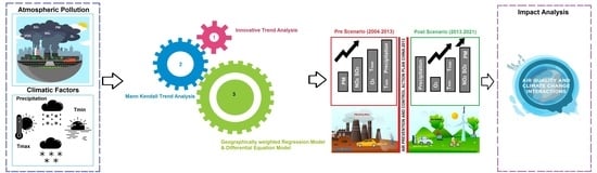
  • To identify the long-term variability of air pollutants (NO2, PM, SO2, and O3) under the pre-scenario and post-scenario scheme to evaluate the comprehensive goal of APPCAP;
  • To determine the long-term trend of climatic factors (tmax, tmin, and precipitation) in compliance with the pollution control policy;
  • To evaluate the spatial climatic contribution of air pollution control management over the past two decades at the national level in China.

2. Materials and Methods
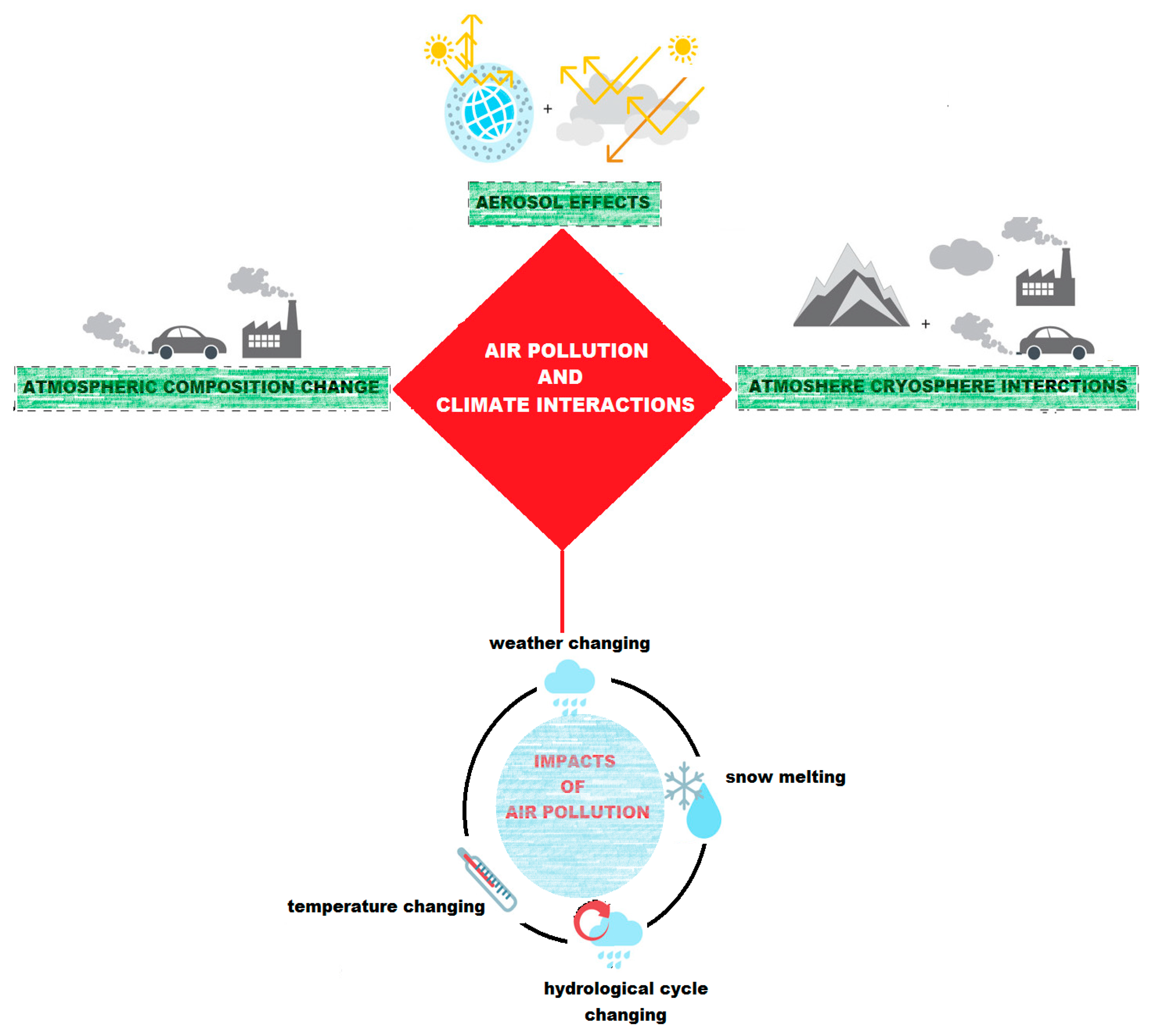
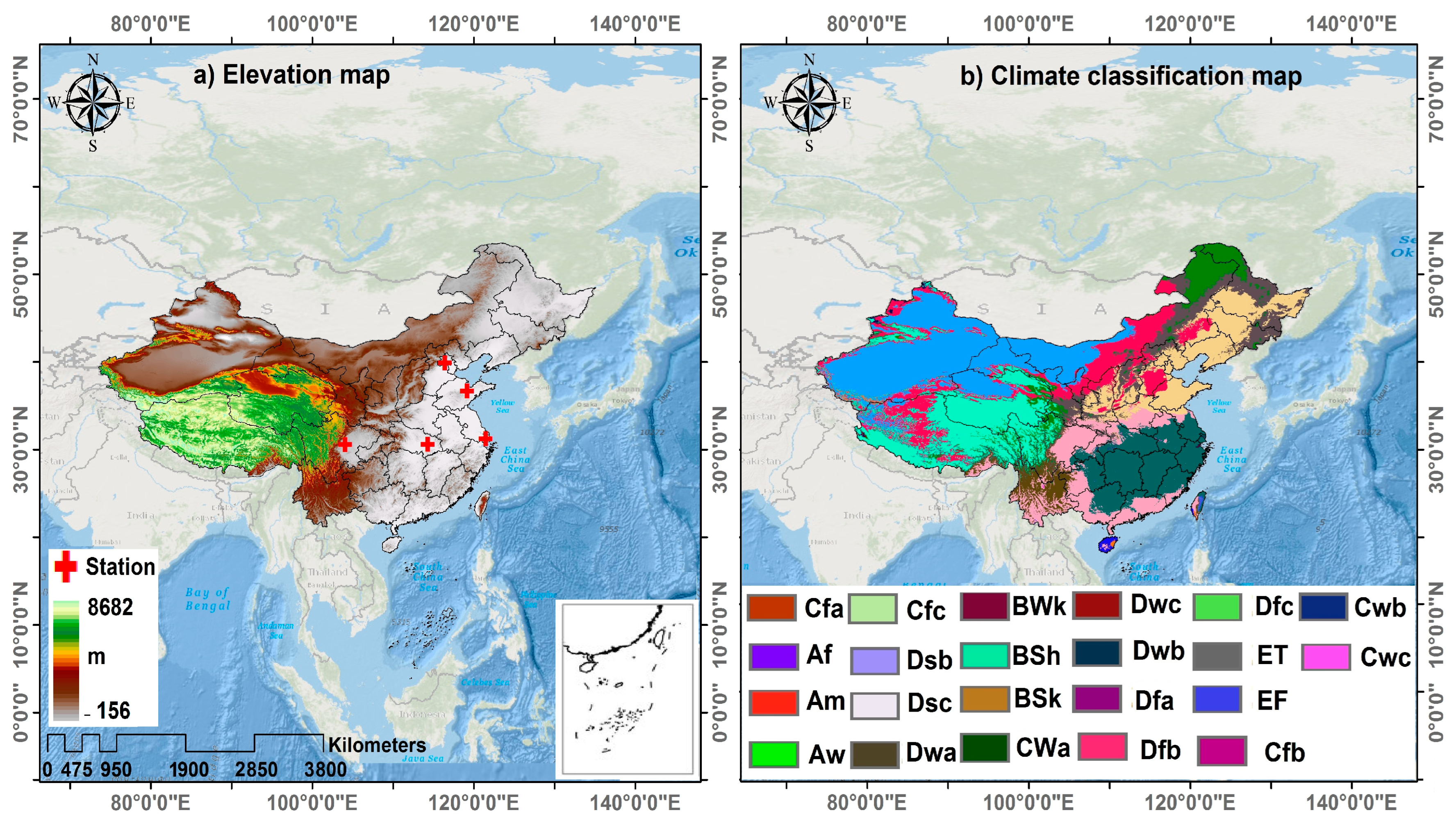
2.1. Study Area

China is a vast and diverse country located in East Asia, covering an area of approximately 9.6 million square kilometers. It has a population of over 1.4 billion people, making it the most populous country in the world. China is divided into six major climate regions, including the tropical, subtropical, warm, middle temperate, cold, and plateau zones [77]. The subtropical zone covers the largest area of China, while the northern part of the country experiences year-round ice and snow. The eastern and southern regions of China are influenced by the Pacific Ocean and are characterized by monsoon climates such as hot, subtropical, and temperate monsoons [78]. These zones are further divided into sub regions based on Figure 2, which shows the location of these different climate zones, providing a useful reference for studying the climate and its impact on different aspects of life in China. Air pollution is a major issue in China, with many cities experiencing high levels of PM, SO2, NO2, and O3. Rapid industrialization, urbanization, and the extensive use of fossil fuels have greatly contributed to China’s severe air pollution problem.
The northern parts of China, including Inner Mongolia and Xinjiang, experience a continental climate, with very cold winters and hot summers. The western region of China, such as Tibet and the Himalayas, has a plateau climate, characterized by low air pressure, thin air, and a large daily temperature range. The eastern and southern regions of China are influenced by the Pacific Ocean, with the monsoon climate dominating the area. The mountainous areas of China have a temperate climate, with cooler temperatures and lower humidity than other areas at the same altitude.

2.2. Data Description

Aura and Terra satellite-based OMI (https://giovanni.gsfc.nasa.gov/, accessed on 12 September 2022) measured the data of three air pollutants, including NO2, SO2, and O3 [79,80,81]. PM data were collected from the NASA SEDAC, which provided global annual PM grids from MODIS, MISR, and SeaWiFS aerosol optical depth, v4.03 [62]. Aerosol optical depth retrievals from multiple satellite algorithms were calibrated based on Aerosol Robotic Network (AERONET) observations (https://sedac.ciesin.columbia.edu (10 September 2022)) [63,64]. Three meteorological parameters (temperature maximum, temperature minimum, and precipitation) were obtained from the Fifth generation (ERA5) (https://www.ecmwf.int/en, accessed on 28 September 2022) [82,83,84] as in the description written for Table 1. Ground measurements were used to compare the satellite-estimated and NASA SEDAC data at some pollution monitoring stations as different locations as indicated in Figure 1. The ground measurements for air pollutants were accessed from a website (http://www.aqistudy.cn/, accessed on 20 February 2023) under the control of the Ministry of Ecology and Environment, China available from 2013.
Only NO2, PM, and SO2 ground concentrations were used to compare the satellite measurements and NASA SEDAC PM, and a high correlation was found between them, as shown in Figure 3.

2.3. Trend Analysis

In the present study, we used two non-parametric statistical approaches to determine whether the meteorological and air pollutants time series were increasing, decreasing, or showing no trend. ITA and MK tests were employed to identify trends in these variables. In particular, the ITA test was used to signify efforts to control air pollution in China. Traditional monotonic trend approaches detect trends using statistical calculations and cannot depict trends in different subcategories of data values. The ITA is an intuitive method for identifying trends in different time series subcategories, regardless of distribution assumptions [85,86,87]. Meanwhile, the MK test assumes that time series have no sequential correlation and is based on the assumption that all data are significant [88]. These techniques are widely used to analyze climatic parameters in particular [82,89].

2.3.1. ITA Trend Analysis

The ITA approach detects disparities in air pollution data time series using a non-parametric approach. Using ITA, the time series is divided into equal halves, and each subseries is sorted in ascending order separately. The first subseries is positioned (Xi; i = 1, 2, …, n/2) on the x-axis, and the second subseries is positioned (Xj; j = 1, 2, …, n/2) on the y-axis based on the Cartesian coordinate system. Both axes must have the same range to interpret the changed information. This approach provides a quick visual understanding of the nature of time series trends. The data values lie on a 1:1 (45°) straight line, indicating that the time series has no trend. The data points that lie above or below the area of triangulation show the increasing or decreasing trends of the time series, respectively [90,91]. The first half of the data points determines the trend change, and the trend indicator is determined by the difference between the two subseries divided by the mean of the first subseries [92].
The longitudinal trend is computed by taking the arithmetic average of the Xj and Xi values at every point in the time series. The vertical and horizontal distance from the linear line is used to calculate the absolute difference. The indicator of the trend [88,91] is computed using the following Equation (1):
S =   2   X j ¯ X i ¯ n
where “S” shows the indicator of the trend, and n is the number of data points at X j ¯   and   X i ¯ , represented as the second and first subseries arithmetic averages, respectively. The positive and negative values of “S” show an increasing and decreasing trend. If the value of observation data is found odd in the original time series, the first observation might be discarded.
The significance of the slope was tested by the method proposed by Sen, and a description of the method was shown in [89].
Confidence limits (CLs) define the significance of the slope of the time series such as if the data points fall out of the CL, then it is statistically significant. To compute the CLs of the slope, it follows a Gaussian probability density function with zero mean and standard deviation as given below:
C L 1 α = 0 ± s c r i × σ s
where 𝛼 is the significance level at a 5% confidence that was used to evaluate the significance of the ITA trend, and s _ c r i is the standard normal PDF; the value of “   s _ c r i ” can be calculated using the following equations:
s _ c r i = Z α 2
where 𝛼 = 1 for confidence level. For example, if we have a 95% confidence level, then the corresponding level of alpha is as follows:
  α   = 1 0.95 = 0.05  
where σ s is defined as:
σ s   = 2 2 n n σ 1 ρ x i ¯ , x ¯ j  
where ρ x i ¯ , x ¯ j is the correlation coefficient between the two mean values.
ρ x i ¯ , x ¯ j = E   X ¯ i X ¯ j E X ¯ i   E X ¯ j     σ x i σ x j

2.3.2. Mann Kendall Trend Analysis

The aforementioned air pollution and meteorological data were evaluated to detect the spatial-temporal variation over the China region using two methods: a non-parametric MK test and Sen’s slope. The negative and positive magnitudes of trends were calculated to find the slope value and detect the trend changes in air pollution and meteorological factors in China. The MK test was used for the inhomogeneous time series data to illustrate the spatial and temporal patterns, and the ZMK test statistic was used [93,94]. The following mathematical equations were used to calculate the MK statistics V(S), S, and standardized test statistic Z:
S = i = 1 n 1 . j = i + 1 n sign   X j X i ,
sign   X j X i = + 1     if   X j X i > 0 0   if   X j X i = 0 1   if   X j X i < 0 ,
V   S = n n 1 2 n + 5 p = 1 q tp   tp 1 2 tp + 5 ,
Z = S 1 VAR S                       if   S > 0 0                                 if   S = 0 S 1 VAR S                       if   S < 0 ,
n is length of time, tp is the tied values for the pth value, and q is the number of tied values, while Xi and Xj are the data values in chronological order. In the current study, the significance of the trend was tested at the Z-critical value > 1.96 with a significance level of 0.05. The null hypothesis of no trend must satisfy the condition if −1.96 > ZMK > 1.96.

2.4. Geographically Weighted Regression Model (GWR)

The GWR model was extensively used in this study to investigate the relationship between the climatic parameters and air pollutants at the national scale of China. GWR modeling is a type of regression modeling with geographically varying parameters (e.g., air pollutants), which differs from conventional regression modeling and was developed to achieve a higher performance in geographical analysis. In general, the GWR model can be expressed by the following Equations (8) and (9) [54,95]:
C i = k β k X i Y i A P k , i + ε i
where C i is the spatial dependent variable at the location 𝑖; X i Y i is the x–y coordinate of the 𝑖th location. β k X i Y i is the coefficient, a varying conditional at kth, and the respective x-y location with the first coefficient by setting A P 0 , i = 1, that is β 0 X i Y i defined as the geographically varying intercept term. A P k , i is the independent variable at kth and the respective x-y location. ε i is the Gaussian error at the x-y coordinate of the 𝑖th location:
C i = β 0 X i , Y i + β 1 X i , Y i   N O 2 + β 2 X i , Y i PM + β 3 X i , Y i S O 2 + β 4 X i , Y i O 3 + ε i
where C i stands for the dependent climatic factors (precipitation, temperature maximum, and temperature minimum). β 0 X i , Y i is the geographical intercept. β 1   to   4 X i , Y i are the respective geographically varying coefficients, which are different from the coefficients of conventional regression. NO2, PM, SO2, and O3 are the independent air pollutants at the x–y coordinate of the 𝑖th location.

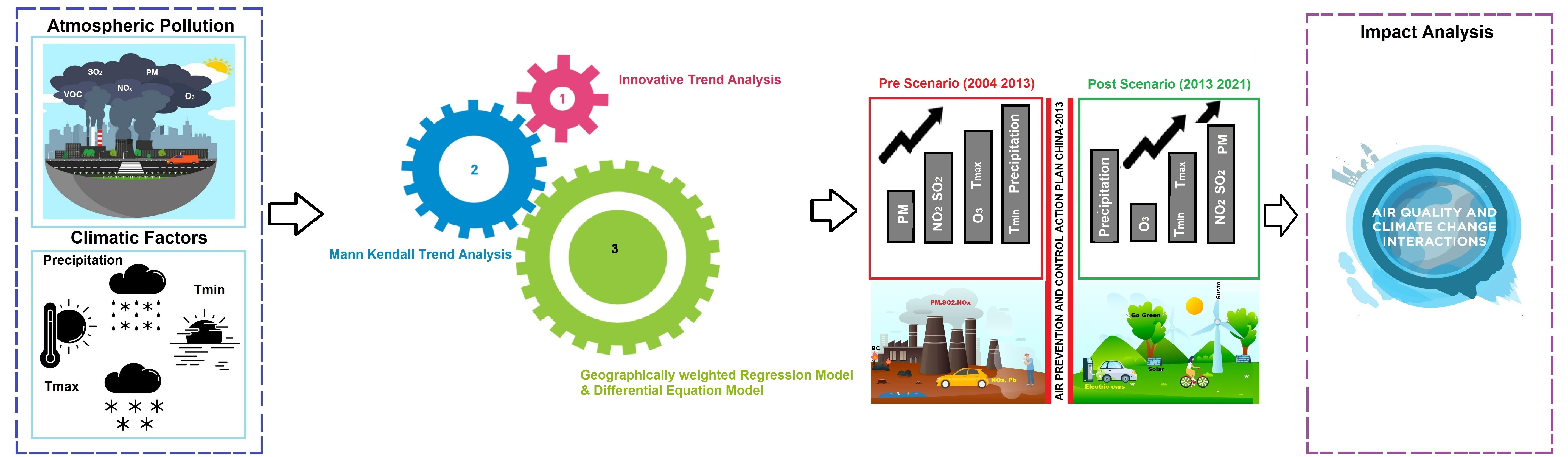
2.5. Impact Assessment of Air Pollution on Climate

The climatic impact of air pollution can be assessed using the following differential Equations (10) and (11):
d C l i m i d t = d C l i m i d P M × d P M d t + d C l i m i d S O 2 × d S O 2 d t + d C l i m i d N O 2 × d N O 2 d t + d C l i m i d O 3 × d O 3 d t
In the above Equation (10), C l i m i means different climatic parameters such as precipitation, temperature maximum, and temperature minimum. This equation is based on the chain rule of calculus, which states that the derivative of a composite function (in this case, “Climi” as a function of “PM, SO2, NO2, and O3” and “PM, SO2, NO2, and O3” as a function of time) is equal to the product of the derivatives of the individual functions. The equation suggests that the rate of change of a climate variable “Climi” can be influenced by changes in an air pollutants “PM, SO2, NO2, and O3”. By understanding the relationship between these variables and their rates of change over time, we can gain insights into how changes in one variable may influence the other. This equation is a simple representation of the complex interactions between the atmosphere, land, and oceans that determine the Earth’s climate. It can be used to investigate the impacts of various human activities, such as emissions of air pollutants, on the climate system.
Δ C l i m i = a × Δ PM + b × Δ S O 2 + c × Δ N O 2 + d × Δ O 3
Equation (11) explains in general that Δ PM ,   Δ S O 2 ,   Δ N O 2 ,   a n d   Δ O 3 are the inter-annual changes while a, b, c, and d mean coefficients.

3. Results

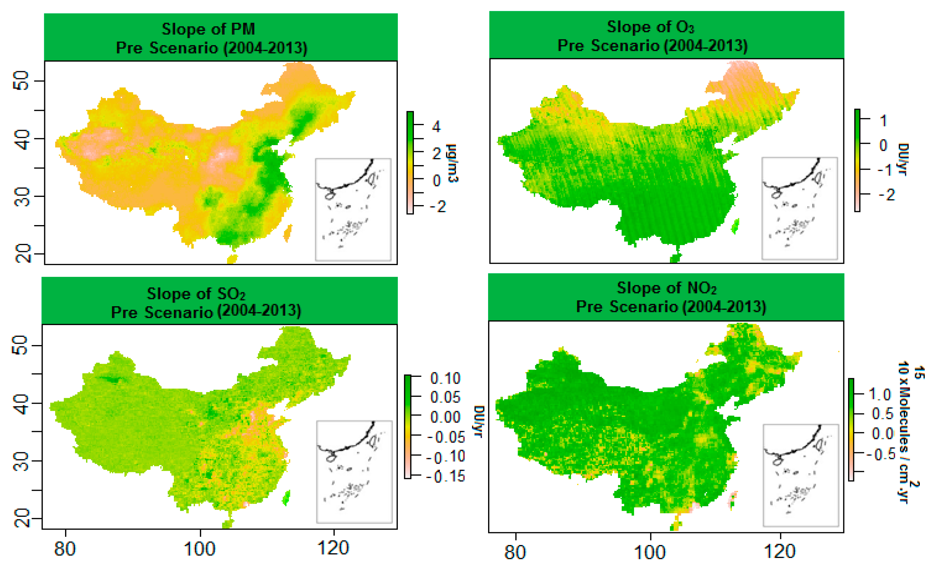
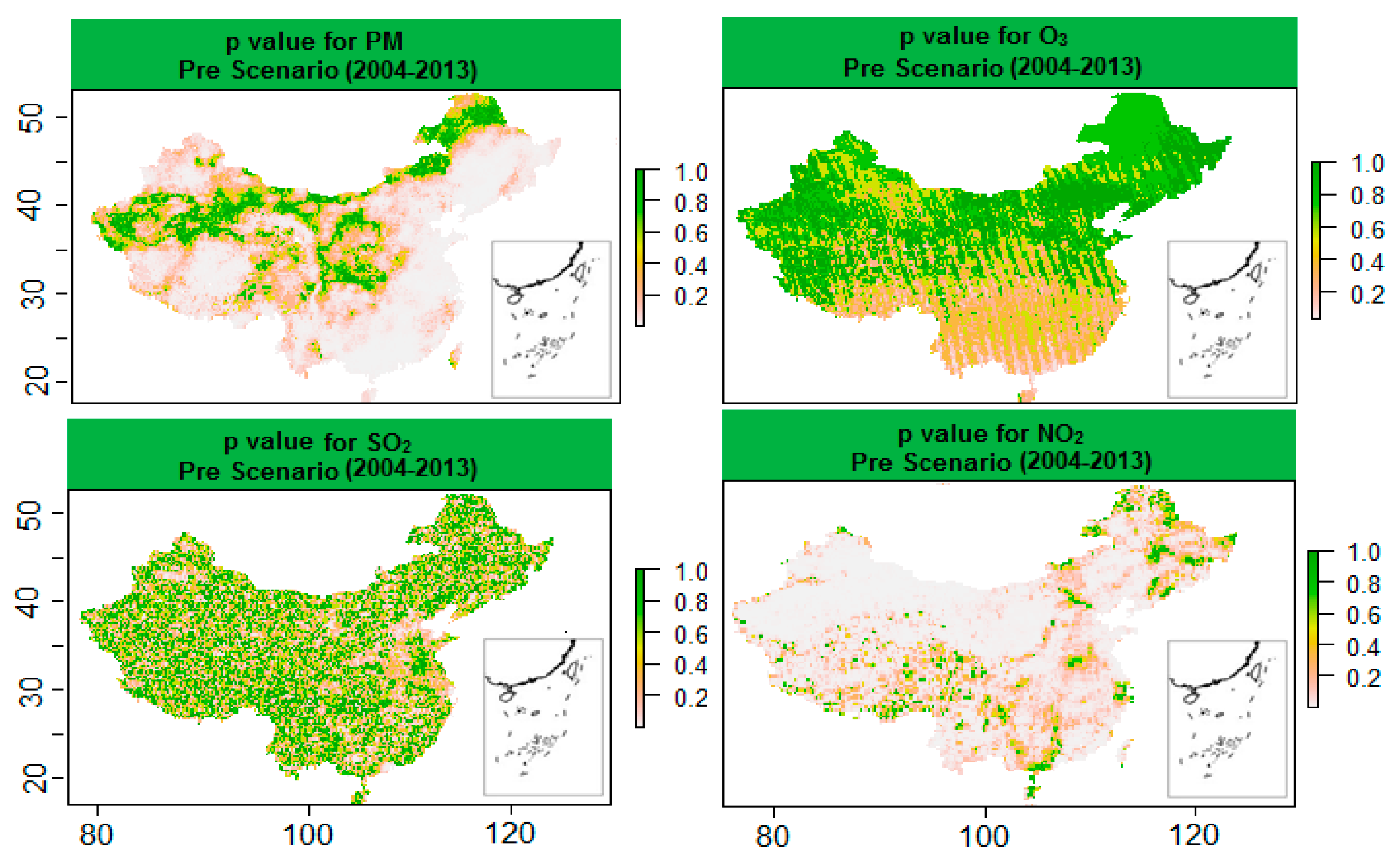
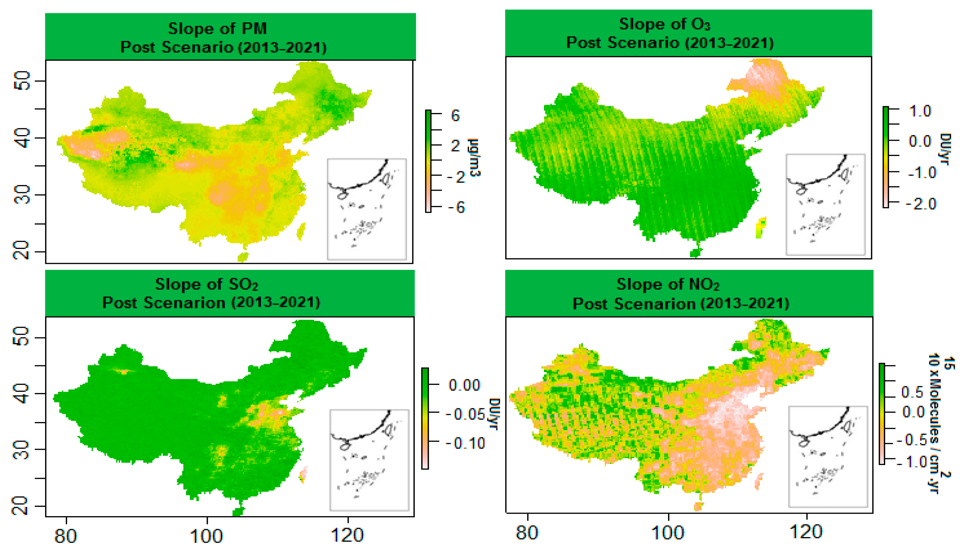
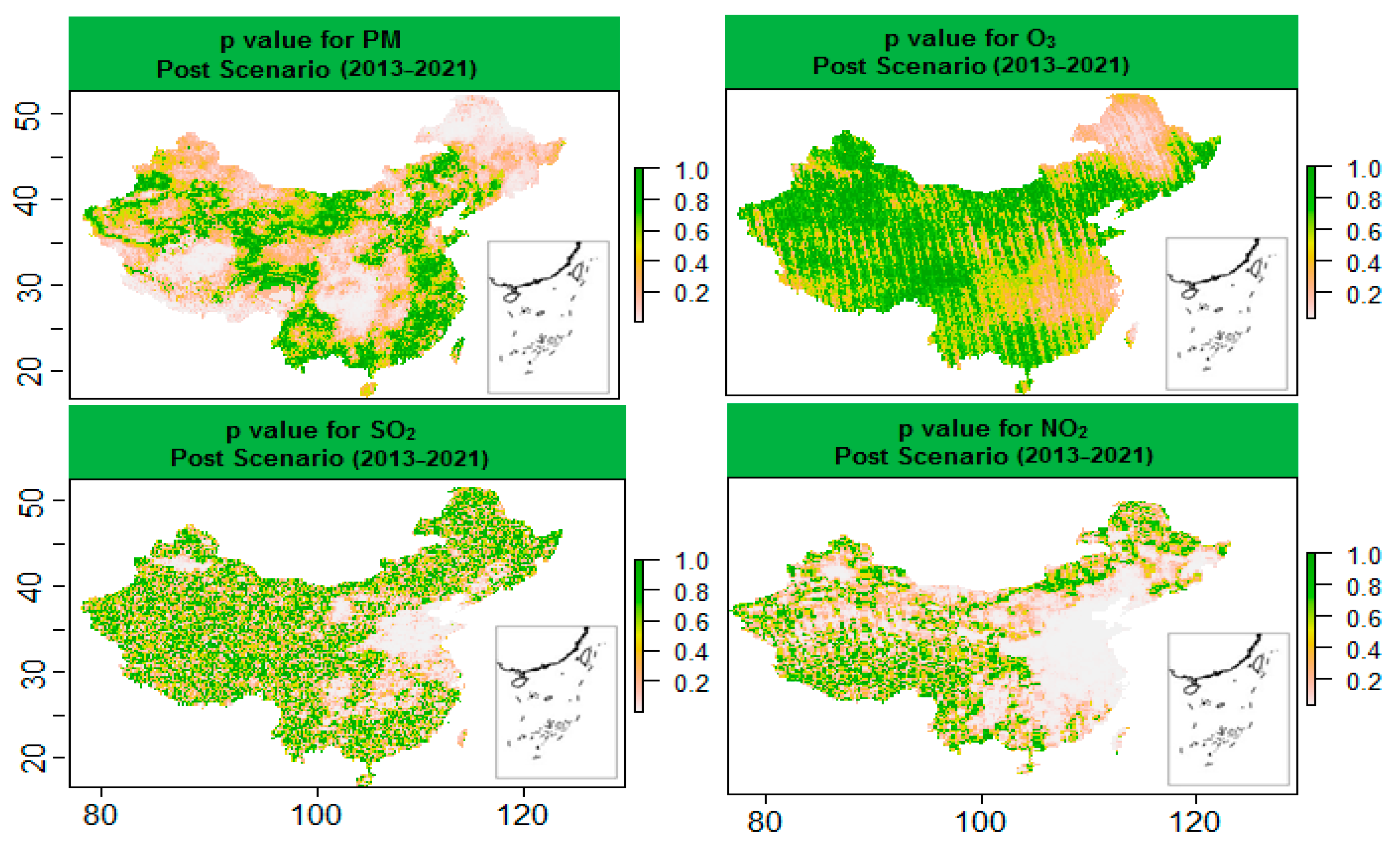
3.1. Trend Analysis of Air Pollution Variation under Pre- and Post-Scenarios

The current study presents the spatiotemporal characteristics of climatic variables and air pollutants from 2004 to 2021 using OMI, SEDAC, and ERA5 data. To analyze the spatial characteristics, we performed a trend analysis on the average annual concentrations of air pollutants from 2004 to 2021. We divided our study period into two scenarios based on APPCAP, namely pre- and post-scenarios, by accounting for the periods 2004–2013 and 2013–2021, respectively. We wanted to ensure the significance of the results of APPCAP in China. During the pre-scenario, it was observed that PM, SO2, and NO2 showed heterogeneous trends, whereas the trend for O3 was homogenous across the study area. Figure 4 shows the most prominent increasing trend for NO2, which was 1.21 × 10¹⁵ molecules/cm2 per year. It is caused by anthropogenic emissions associated with economic growth, including traffic flow and urbanization [60].
In the case of PM and SO2, the increasing trend was 4 µgm–3/year and 0.1 DU/year, respectively, during 2004–2013. In the pre-scenario group, the highest increasing trend for PM was recorded in northeast, east, and southeast China. For O3, the trend over China was increasing, with the maximum value being 1 DU/year. On the other hand, the highest decreasing trend was recorded at 1.0 × 10¹⁵ molecules/cm2 per year for NO2 cross ponding to different hotspots in China.
The p values for PM and NO2 were highly significant over most of the parts of the study region, as illustrated in Figure 5, whereas a mixed trend of p-value variation was observed for SO2 and O3.After adopting the APPCAP (post-scenario), it was observed that PM and NO2 showed a significantly decreasing trend in most of the part of China, whereas the trend for O3 was still increasing in China.
Figure 6 shows the most prominent decreasing trend, as the trend for NO2 was 1.21 × 10¹⁵ molecules/cm2 per year. In the northwest and north China, the trend was mixed for NO2, while the northeast China PM trend increased after adopting the APPCAP. In the case of O3, the trend decreased in the north part, while the rest of the area showed an increasing trend. The decreasing trend of O3 was 2.0 DU/year during 2013–2021. In the post scenario, the trend for SO2 was random, and a decreasing trend was found in central China, including the Shandong and Beijing areas. The highest decreasing trend for SO2 was 0.10 DU/year, while the decreasing trend was recorded for PM in northeast, east, and southeast parts of China, with a peak value of 6 µgm−3/year. In contrast, O3 showed an increasing trend with a maximum value of 1.2 DU/year. The highest increasing trends recorded were 0.05 DU/year and 1.21 × 10¹⁵ molecules/cm2 per year for SO2 and NO2 in China. From Figure 7, the p values showed that the decreasing trend for PM and NO2 was highly significant in the study region, whereas the increment in O3 pollution was highly significant during the post-scenario period.

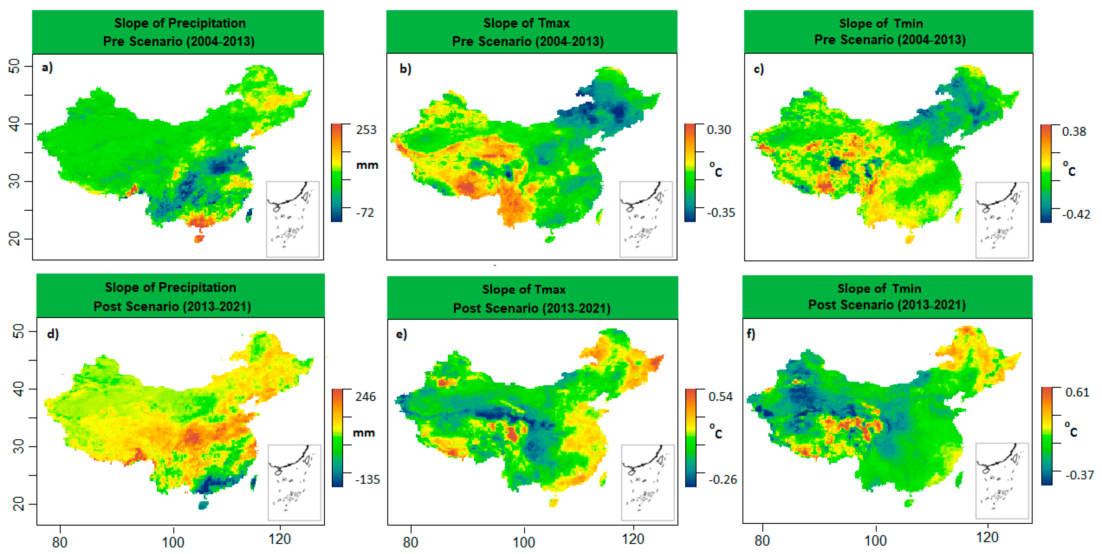
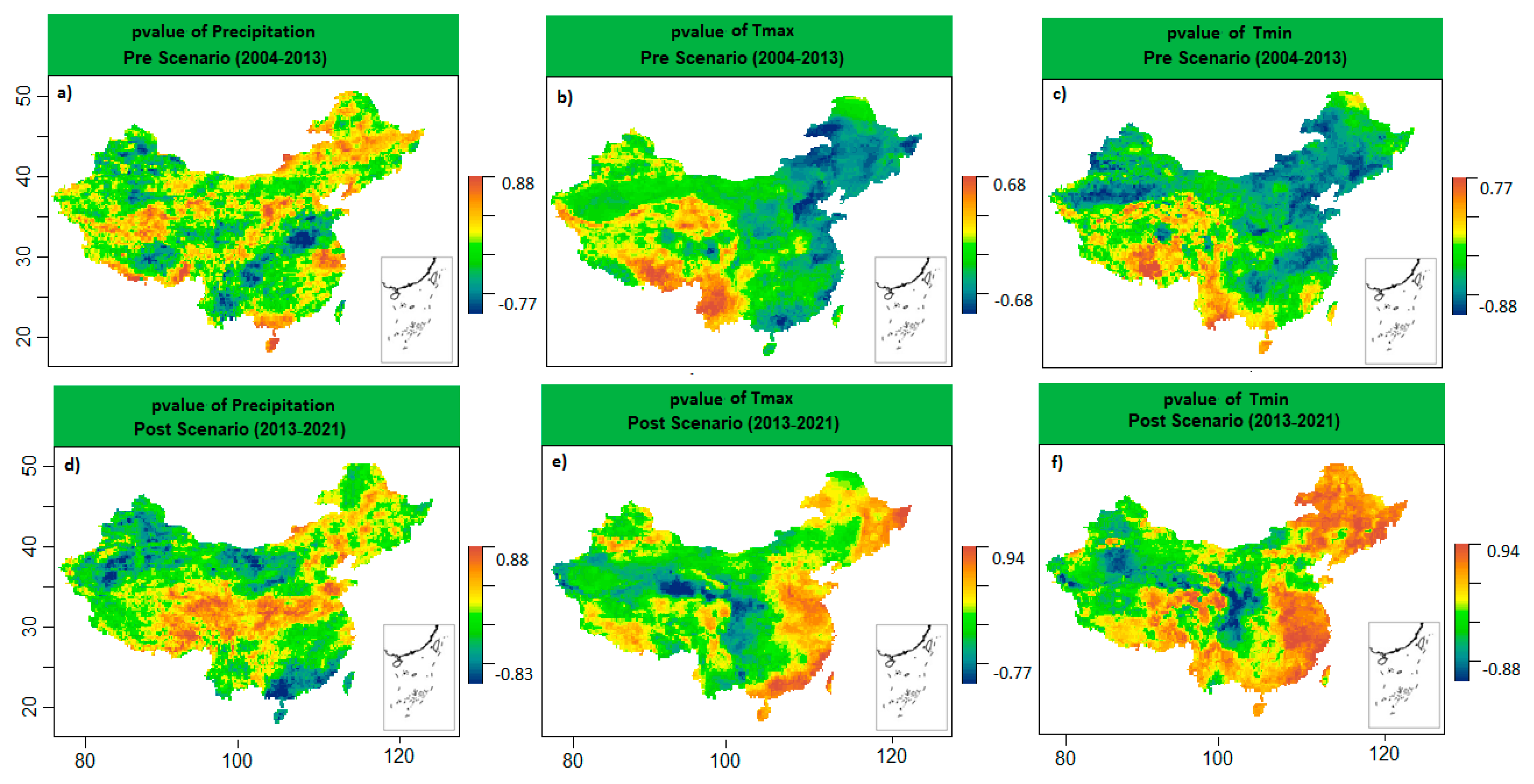
3.2. Trend Analysis of Climatic Factors Variation under Pre and Post Scenarios

Figure 8 shows the spatial variation in trends for climatic parameters, including tmax, tmin, and precipitation. In general, all parameters showed an increasing trend across the study region. During the pre-scenario, tmax and tmin showed a prominent increasing trend, while precipitation showed a less significant increasing trend. tmax showed the maximum increasing trend of 0.30 °C/year, while tmin represented 0.38 °C/year. The precipitation trend also increased, but it was prominent in the north and southeast regions of China, where it increased by value 253 mm/year. However, a prominent decreasing trend was found along the Shandong region to the south part. The precipitation trend decreased by 72 mm/year. In the case of tmax, the trend did not significantly increase in the northern region, whereas tmin showed a decreasing trend in the same region of China. The maximum decreasing trend for tmax and tmin was 0.35 °C/year and 0.42 °C/year, respectively. The trend variation in tmax, tmin, and precipitation was highly significant at p < 0.05 across the study area, as shown in Figure 9. After adopting the APPCAP, the trend variation was in contrast to the pre-scenario trend analysis results. Precipitation and tmax showed increasing trends with maximum trend values of 246 mm/year and 0.54 °C/year, respectively. The tmin trend seemed to slightly increase by 0.61 °C/year, especially in the north and southwest parts of China. In contrast, the precipitation trend decreased by 135 mm/year, particularly in the southeast part of China. Furthermore, tmax and tmin showed a decreasing trend over 2013–2021 with a magnitude of 0.26 °C/year and 0.37 °C/year, respectively.

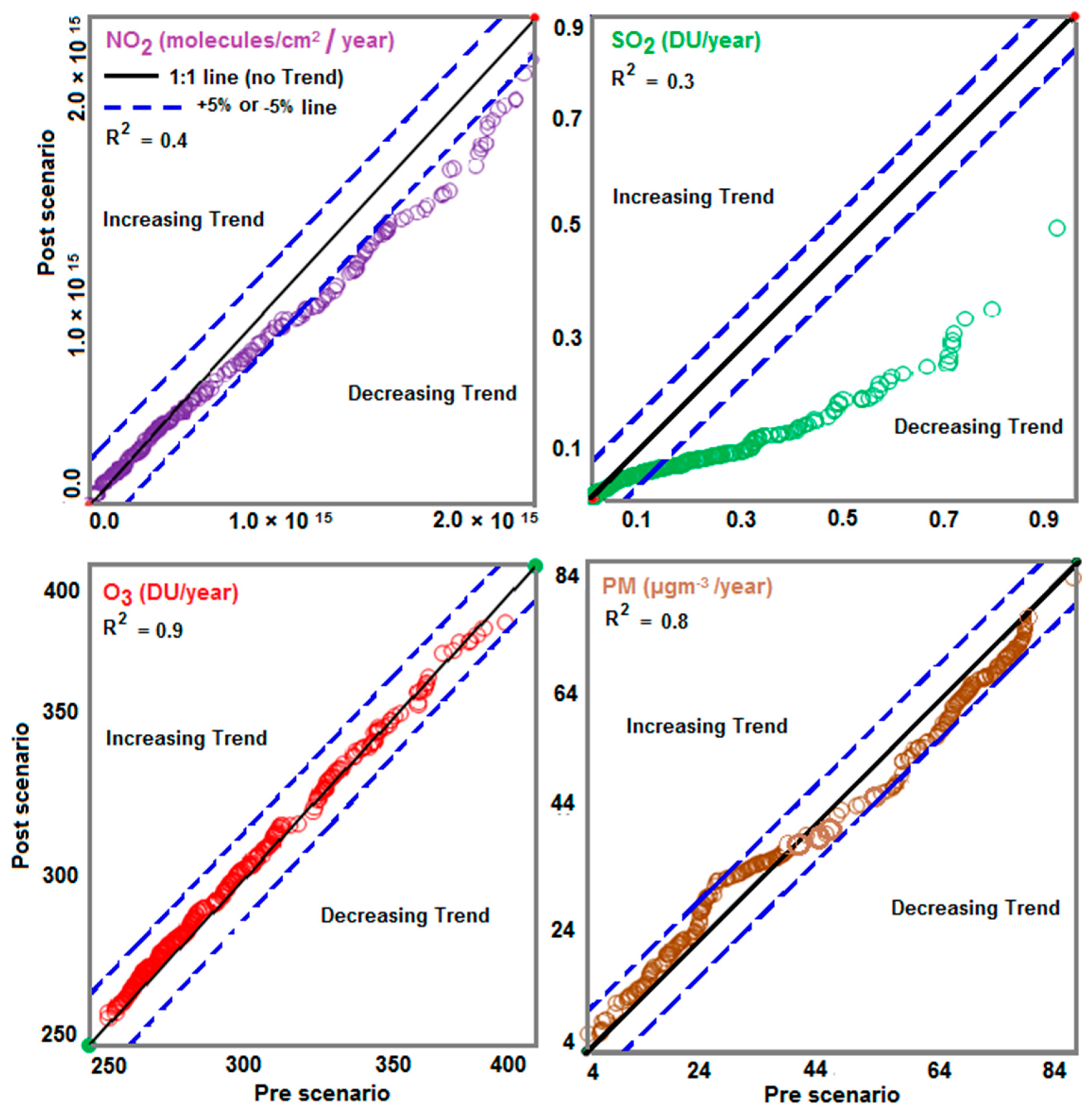
3.3. ITA Analysis for Air Pollution Variation under Pre and Post Scenarios

The annual variations in air pollutants were studied to analyze the impact of APPCAP on air pollution reduction. The ITA analysis showed an increasing or decreasing trend over two decades, during pre-scenario and post-scenario periods. A combination of increasing and decreasing trends for data points above the 5% range from the 1:1 line exhibited a significant trend. The results showed that, overall, NO2, PM, and SO2 decreased after adopting APPCAP across China. Figure 10 suggests that air pollutants (NO2, PM, SO2, and O3) significantly decreased. The results also showed that NO2 data points fell within the −5% range, showing a decreasing trend during 2004 and 2021. The statistics for NO2 exhibited significant negative values of ITA D. The O3 data points were mostly on the diagonal line, indicating no trend/zero trends. The SO2 data points fell above −5%, indicating that it decreased after adopting APPCAP. However, it was concluded that the decreasing trend of SO2 was not significant over the period.

3.4. Impact Analysis of Air Pollutants on Climatic Factors before and after APPCAP

The impact analysis of air pollutants was investigated using the GWR model and differential Equations (8)–(11). We performed a spatial distribution analysis on the outputs from the differential equations to investigate the climatic impact of air pollution over two scenarios based on APPCAP in China.

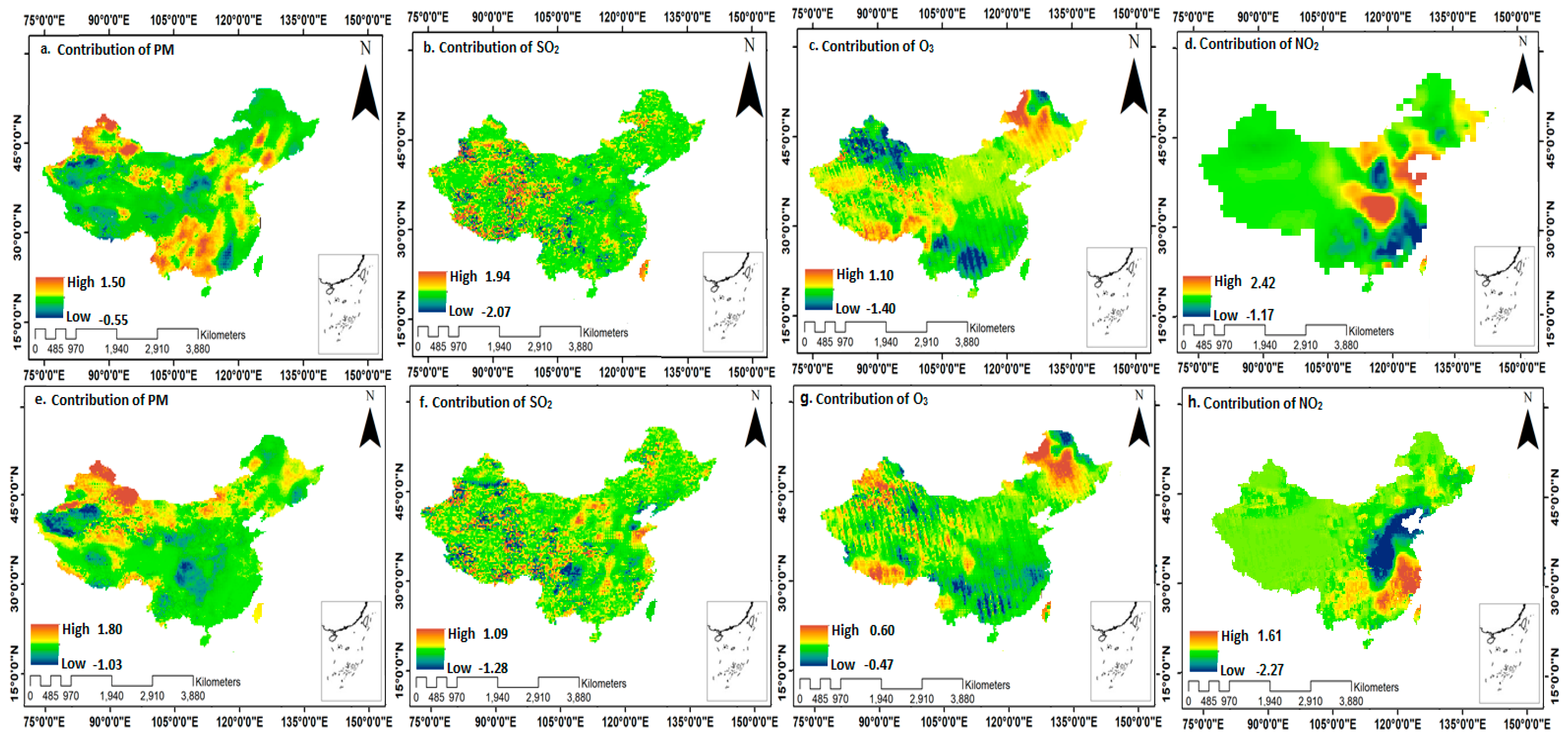
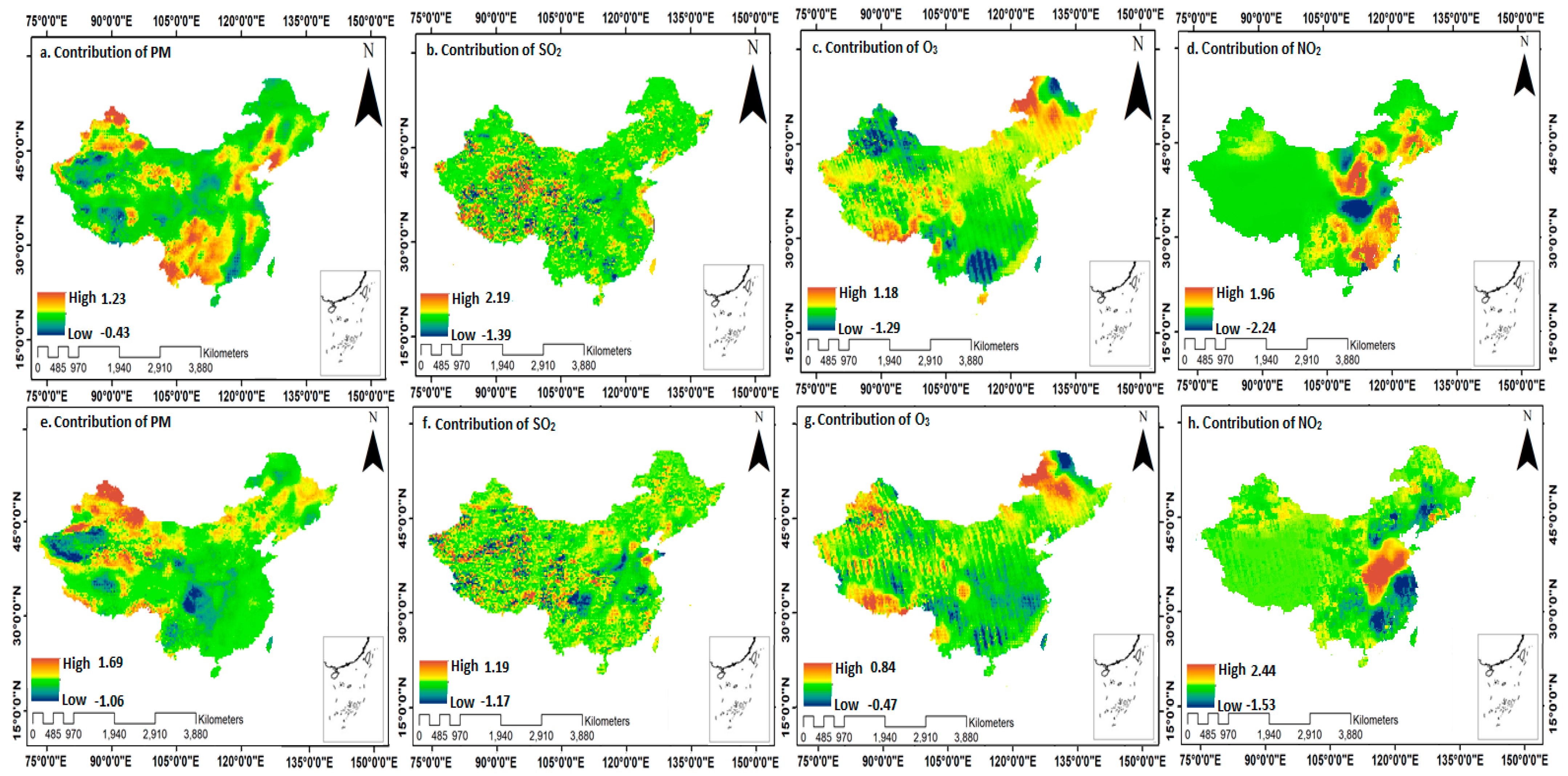
3.4.1. Air Pollutant’s Contribution to Temperature Maximum Patterns

The spatial characteristics of the contribution of air pollutants to tmax patterns for the pre-scenario and post-scenario periods are represented in Figure 11. Higher positive values show a greater influence on increasing tmax over the study period. For the pre-scenario period, NO2 had a higher value and increased tmax by 2.42 °C, while O3 had a lower positive value of 1.10 °C over a decade. In the case of SO2, the contribution pattern was random. In contrast, SO2 had higher negative values and decreased tmax by 2.07 °C, while PM showed the lowest negative contribution with 0.55 °C over China. PM caused an increase in tmax in central east and southeast parts of China, as shown in Figure 11a. After adopting the APPCAP (post-scenario), PM showed the highest positive contribution to increasing tmax by 1.80 °C, while O3 contributed the lowest positive value of 0.60 °C. SO2 showed random spatial patterns of increasing or decreasing tmax over the whole study area. NO2 contributed more to decreasing tmax by 2.27 °C, and spatial patterns showed that central east China was reducing tmax, as shown in Figure 11h.
O3 reduced tmax in the southern part of China. The contribution pattern of O3 indicated the lowest negative contribution to decreasing tmax by 0.47 °C. In general, a comparison of all air pollutant’s contributions indicated that, during the pre-scenario period, tmax positively changed by 2.42 °C, followed by NO2, while in the post-scenario period, tmax positively changed by 1.80 °C, followed by PM. In contrast, the highest negative tmax change was by 2.07 °C, followed by SO2, and 2.27 °C followed by NO2, respectively. NO2 and PM particles can contribute to global warming by trapping the heat in the atmosphere. They cause the warming effect on the atmosphere by absorbing the sunlight and re-emitting it as heat, leading to a rise in the temperature. The current effect is more in urbanized areas, where there are high traffic and industrial emissions. Further, NO2 may also react with chemicals in the atmosphere to form secondary pollutants such as O3, which can increase warming. Moreover, O3 leads to an increase in temperature. SO2 is primarily released from the burning process and volcanic eruption. It has harmful effects on human health as well as the environment. However, SO2 emissions contribute to warming the atmosphere because it can react with other chemicals in the atmosphere to form sulfate aerosols and lead to an increase in temperature. This effect is more prominent in areas with high concentrations of SO2, such as power and industrial plants. Overall, the pollutants significantly impact the temperature maximum, particularly in areas with high concentrations. The effect of the air pollutants on tmax depends on the concentration level, size of the particles, as well as other factors such as location and weather conditions.

3.4.2. Air Pollutant Contribution to Temperature Minimum Patterns

In this section, the spatial characteristics of the contribution to tmin changes for the pre-scenario and post-scenario periods are represented in Figure 12, which shows the spatially interpolated geographical air pollution contribution to climatic factors (tmin). The northern, western, and southeastern parts of China indicated a position association with air pollutants during the pre-scenario period (2004–2013). Figure 12a,d shows the higher positive influence on increasing tmin by 2.19 °C, followed by SO2, while NO2 had the second highest contribution to change in tmin by 1.96 °C during the pre-scenario period. The northeastern and southern parts indicated the rise in tmin due to the variation in PM. NO2 caused higher tmin changes over the north, central, and southeast parts of China. In contrast, NO2 contributed to a higher negative contribution to decrease tmin by 2.24 °C, while PM had a lower negative contribution with a value of 0.43 °C over a decade. Figure 12d indicates that NO2 was mainly responsible for decreasing tmin mainly in the central part of China. O3 and SO2 had mixed patterns for changing tmin (Figure 12b,c).
In the post-scenario period, the west, north, and central parts of China showed an increasing contribution to tmin changes. NO2 showed the highest positive contribution to increasing tmin by 2.24 °C, while O3 had the lowest positive contribution with 0.60 °C. The second highest positive contribution to increasing tmin was with PM (1.69 °C). SO2 and O3 showed random spatial patterns to increase or decrease tmin over the whole study area. NO2 had a positive contribution in central east China, as shown in Figure 12h. In contrast, NO2 had the highest negative contribution for reducing tmin by 1.53 °C in the northeast and southeast parts of China.
Moreover, O3 contribution patterns indicated the lowest negative contribution to decreasing the tmin by 0.47 °C. O3 reduced tmin in the east-southeast part of China during the post-scenario period. Overall, a comparison of all air pollutants contributions indicated that, during the pre-scenario and post-scenario periods, the tmin changed the highest positively by 2.19 °C followed by the SO2, while it was 2.44 °C followed by NO2 during the pre-scenario period. In contrast, tmin has the highest negative change by 2.24 °C, while it was 1.53 °C followed by NO2 in the case of the pre- and post-scenario periods, respectively. NO2 has direct and indirect impacts on temperature minimum. It can have a warming effect. NO2 absorbs sunlight and heat in the atmosphere that can lead to an increase in temperature, especially at night. It is important to note that impacts of SO2 on tmin depend on the different factors such as season and altitude. The sulfate aerosols reflect solar radiation and reduce the energy on the Earth’s surface. This phenomena causes a cooling effect on temperature, including tmin. Moreover, NO2 causes the urban heat island effect, where cities experience higher temperatures than surrounding rural areas due to human activity and the built environment. This effect can further increase the minimum temperature in urban areas, leading to a range of health and environment impacts.
This warming effect can have several consequences, including the melting of snow and ice, changes in precipitation patterns, and alternations in plant growth and ecosystem functioning.

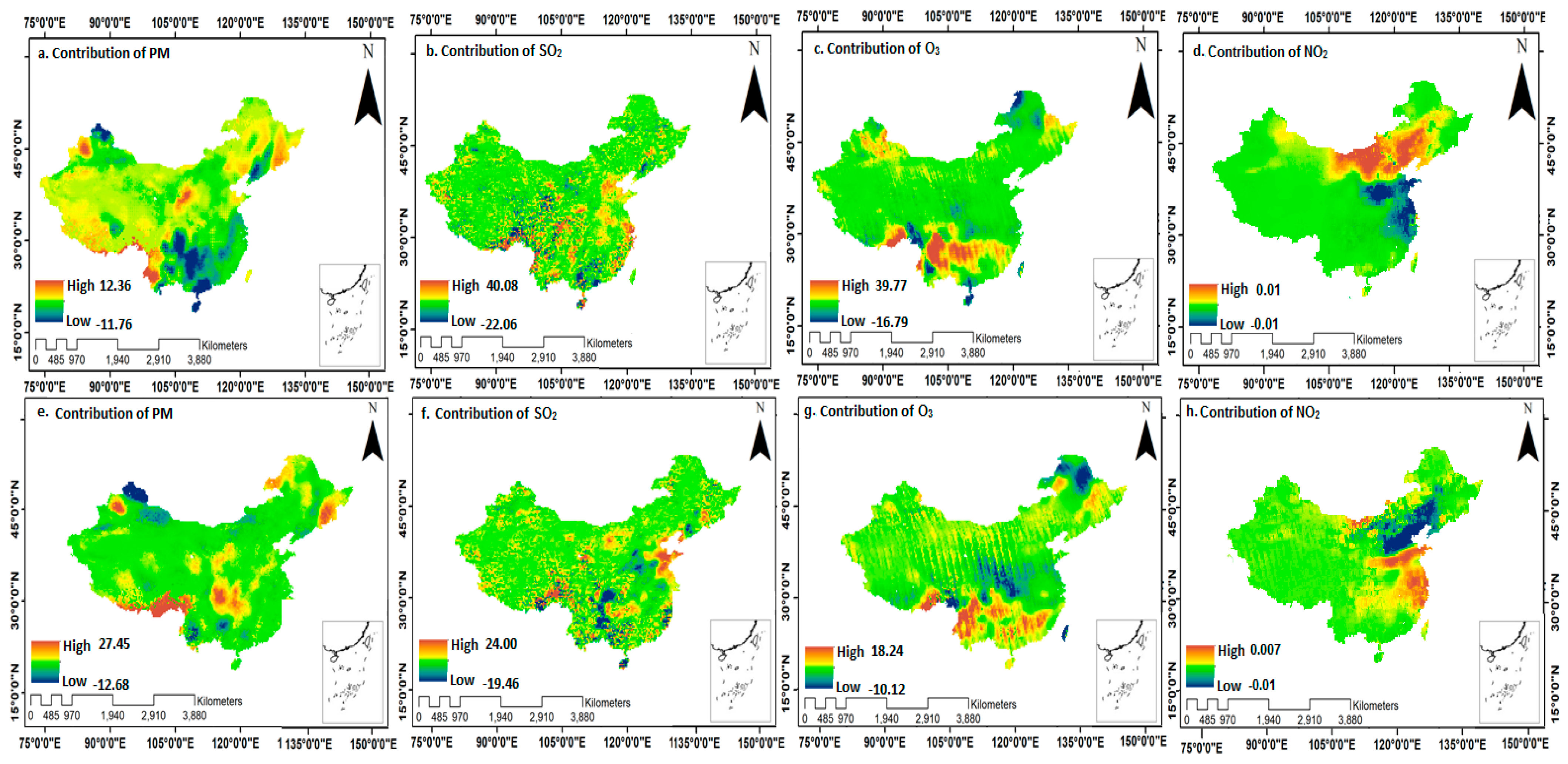
3.4.3. Air Pollutant Contribution to Precipitation Patterns

Figure 13 shows spatial maps of the contribution of air pollutants in changing precipitation patterns over China in the pre- and post-scenario periods. Figure 13b,c shows the highest positive influence on precipitation, with an increase of 40 mm, followed by SO2, while O3 had the second highest contribution to changes in precipitation, with an increase of 39 mm during the pre-scenario period. The central-eastern part indicates the rise in precipitation due to variations in SO2, while O3 caused higher precipitation changes over the Southern part of China. In contrast, SO2 had a negative contribution to decreasing precipitation by 22 mm, while NO2 had lowest negative contribution, with a value of 0.01 mm over a decade. Figure 13b,d indicates the lower precipitation hotspots in the south of China caused by SO2, while NO2 showed hotspots in the east of China, respectively.
In the post-scenario period, the south, east, and central parts of China showed increasing contributions to precipitation alteration. PM made the highest positive contribution to increasing the precipitation by 27 mm, while NO2 had the lowest positive contribution, with 0.007 mm. The second-highest positive contribution to raising precipitation was with SO2 (24 mm). The PM contribution was positive in the central part of China, as shown in Figure 13e. In contrast, SO2 had the highest negative contribution to reducing the precipitation magnitude by 19 mm in the central east (Shandong) part of China. Moreover, NO2 contribution patterns indicated the lowest negative contribution to reducing precipitation by 0.01 mm. NO2 reduced the precipitation in the north part of China during the post-scenario (2013–2021). Overall, a comparison of all air pollutant contributions indicated that during the pre-scenario period, the highest positive precipitation change was by 40 mm followed by SO2, while it was 27 mm followed by PM in the case of the post-scenario period. In contrast, the highest negative precipitation change was by 22 mm, while it was 19 mm followed by SO2 during the pre- and post-scenario periods, respectively. SO2 and PM had significant impacts on the precipitation pattern and environment. SO2 reacts with other chemicals to produce sulfate aerosols that may affect precipitation in different ways. SO2 affects the precipitation pattern by altering the formation of clouds. Sulfate aerosols act as cloud condensation nuclei, which are important for the formation of clouds. PM particles promote the formation of clouds and change their properties through cloud condensation nuclei. However, these particles may affect the properties of clouds, including droplet size, their reflectivity, and the amount of precipitation they produce. As a result, the timing of precipitation as well as the pattern is affected. Additionally, SO2 may impact precipitation patterns through its interactions with other atmospheric chemicals.
As an example, SO2 reacts with nitrogen oxides to create fine PM particles that significantly affect precipitation patterns, in particular, the areas with high concentrations of both SO2 and NOx. PM emissions from urban and industrial areas can lead to forming urban heat islands, which alter local wind patterns and precipitation by changing the moisture content and temperature of the air.

4. Discussion

The State Council issued an action plan, APPCAP, to combat air pollution in 2013, which became the most ambitious policy to control air pollution concentrations [30,72]. APPCAP aimed to improve the following aspects: (1) control air pollution, (2) control pollution substances, (3) diversify air pollution control strategies, and (4) optimize pollution management mode [71,96,97]. The current study divided the entire study period into two separate scenarios to better comprehend the promising efforts of China: the pre-scenario (before APPCAP) and post-scenario (after APPCAP) periods. The APPCAP is a significant development in China’s efforts to curb air pollution, and motivates researchers to assess the implications of air pollution’s management at the national level. MK trend analysis was performed before and after APPCAP implementation on mean annual data. ITA is an intuitive method used to identify trends in different time series subcategories and can be applied irrespective of distribution assumptions [85,86,87], while the MK test assumes that time series have no sequence correlation and are least-based and all data are significant [88]. During the pre-scenario period, trend analysis results on PM, SO2, and NO2 showed heterogeneous trends, whereas the trend for O3 was homogenous. The most prominent increase in NO2 concentration was 1.21 × 10¹⁵ molecules/cm2 per year [64,98,99]. In the case of PM and SO2, the increasing trend was 4 µgm−3/year and 0.1 DU/year [88]. Northeastern, eastern, and southeastern China showed the highest increasing trend for PM in the pre-scenario period. For O3, the trend increased across the region with a maximum value of 1 DU/year in the pre-scenario period.
In light of stringent clean air pollution actions, including APPCAP, adopted in China since 2013 (post-scenario), data analysis showed that PM and NO2 had significantly decreasing trends in most of China, while the trend for O3 did not reduce considerably and is still escalating [100,101]. In the post-scenario period, Beijing, Shandong, and other areas of central China showed a random and declining tendency for SO2 [102], with the greatest rate of decline for SO2 being 0.10 DU/year.
The spatial variation of the trend for the climatic parameters, including tmax, tmin, and precipitation, increased across the study region. During the pre-scenario period, tmax showed a decreasing mean annual trend of 0.025 °C/year, and tmin represented 0.02 °C/year, respectively, while precipitation had an increasing mean annual trend by a value of 90 mm/year. After adopting the APPCAP, trend variation was in contrast to the pre-scenario period for temperature trend analysis results. During the post scenario period, precipitation, tmax, and tmin showed increasing mean annual trends by 55 mm/year, 0.14 °C/year, and 0.12 °C/year, respectively, and were highly significant at (p < 0.05). Overall, tmax and tmin increased while the precipitation reduced.
A comparison of the effects of air pollution on climate between the pre- and post-scenario periods was analyzed for a two-decade period using ITA to determine whether there was an increasing or decreasing trend. The results showed that, when China adopted the APPCAP, overall concentrations of NO2, SO2, and PM declined. Figure 10 indicates that the levels of airborne pollutants (NO2, SO2, and PM) dramatically decreased. NO2 data values above the −5% range showed a declining trend between 2013 and 2021, and NO2 statistics exhibited significant negative values for ITA. However, despite the massive reduction in NOx emissions from power plants, vehicle emissions continued to increase. Both on- and off-road vehicles significantly contribute to air pollution, and multiple studies have revealed a strong correlation between rising vehicle traffic and air pollution in Chinese megacities [103,104,105,106]. Since the 1990s, the central government has implemented integrated emission control policies to reduce vehicle emissions, including emission standards for new vehicles, emission controls for existing vehicles, modifications in fuel quality, the promotion of advanced vehicles, sustainable transportation, and traffic management programs [107].
O3 data points mostly fall on the (1:1) line, indicating no trend/zero trends. According to Liu [108], the sources of the ozone and its variation in concentrations in China, substantial declines in PM, and SO2 emissions lead to a rise in urban O3 due to the dynamic interaction between aerosols, radiation, and chemical reactions. O3 concentrations also increase in the southwest due to climatic factors [109]. Additionally, several studies found that reducing the concentration of NOx increases the amount of O3. During the COVID-19 lockdown, the transportation sector shutdown resulted in a reduction in NOx, which decreased the neutralization of NO into O3, which raised the concentration of O3 [110,111].
The SO2 data points were above −5%, indicating that it started to decline after the APPCAP was implemented. Additionally, it was determined that the decreasing tendency of SO2 over the period was significant and it was in line with findings of [97]. China’s environmental regulations resulted in significant reductions in SO2 emissions, but overall, coal consumption has continued to rise. Since 1996, reducing SO2 emissions from major industries, including coal-fired thermal power and iron/steel plants, has been top priority. The installation and strict management of online monitoring equipment in the main industries have become mandatory, and different policies and programs have been implemented during previous Five-Year Plans [107,112].
Our study has certain limitations. We examined the long-term changes in air pollutants and climatic factors, as well as their association based on different statistical models. The APPCAP adaptation resulted in an increase in tmin and precipitation. The rise in tmin may result in local warming in China for the most part, which requires more efforts to combat climatic change. To this end, there is a need to focus on the mechanisms underlying these regional climate changes, based on seasonal variation. The climatic effect of air pollution along seasonal variation remains unexplored, and coupling regional climate models to analyze the radiative effects of China’s emission reductions.

Climatic Impact of Air Pollutants for Pre and Post Scenarios

The current study describes the climatic changes due to variations in air pollutants in response to the adoption of the APPCAP. In the pre-scenario period, most of the air pollutants showed positive contributions to changing the climate. For example, O3 played a role in reducing tmax (tmin) with a value of 0.15 °C (0.05 °C) and increasing precipitation with a value of 11mm, as shown in Table 2. PM showed a positive relationship with all climatic parameters with values of 0.47 °C (tmax), 0.41 °C (tmin), and 0.31 mm (precipitation). The analysis showed that NO2 had positive and negative relationships with tmax (precipitation) 0.62 °C (0.1mm) and tmin (0.14 °C), respectively. SO2 showed an increasing contribution with tmin (precipitation) 0.41 °C (9mm), while decreasing with tmax (0.06 °C).
During 2013–2021 (post scenario), most of the air pollutants (PM, SO2) showed positive contributions to alter the climatic pattern including tmax, tmin, and precipitation. The analysis showed that PM had a positive relationship with tmax (tmin) 0.38 °C (0.31 °C), and precipitation (7.38 mm). NO2 showed an increasing contribution with tmin (precipitation) 0.35 °C (0.001 mm), while decreasing with tmax (0.33 °C). Moreover, SO2 indicated an increasing contribution to tmin (precipitation) 0.02 °C (2.2 mm), while decreasing with tmax (0.09 °C).

5. Conclusions

In summary, when China adopted the APPCAP, NO2, SO2, and PM concentrations declined dramatically. According to ITA, NO2 data values above the –5% range showed significant declining trend between 2013 and 2021. Although O3 concentrations have gradually increased, the air quality in most cities has immensely improved as a result of the stringent control measures by the State Council. The O3 data points are mostly on the (1:1) line, which means that there is no trend/zero trends. The decreasing tendency of SO2 over the period is not significant. Despite the tremendous progress made in reducing air pollution, PM and O3 concentrations continue to be considerably above WHO guidelines. More efforts are required to focus on the research and development of new methods to address these ongoing challenges in air pollution emissions. The MK test investigated that all pollutants showed an increasing trend for pre-APPCAP, while showing a decreasing trend, except for O3, during the post-APPCAP period. For climatic factors, the MK test showed an increasing trend of precipitation and tmin for the post-APPCAP period.
We used GWR and differential equation models to identify the climatic impact of air pollution before and after the implementation of APPCAP in 2013 to combat air pollution. Two scenarios based on APPCAP were made to account for the air pollution variation in China during 2004–2021. The contributions of the most influential air pollutants were calculated using the GWR and differential equation models. In the pre-scenario period, NO2 contributed to increasing the mean maximum air temperature (tmax) by 0.62 °C, PM contributed to raising tmin by 0.41 °C, while O3 reduced tmax(tmin) by 0.15 °C (0.05 °C). PM increased tmax and precipitation with magnitudes of 0.38 °C and 7.38mm, respectively, while NO2 contributed to increasing tmin by 0.35 °C during the post-scenario period. In particular, the post-scenario period led to increases in tmin and precipitation across the country. The current study findings explain the significance of APPCAP and its role in changing the regional climate of China. Policymakers must implement measures to reduce emissions and maintain the climate warming level across the region. In the future, China needs to introduce more renewable energy to dominate the coal energy system, which may help with national and international climate mitigation measures.

Author Contributions

Conceptualization, B.C. and A.D.; methodology, A.D.; software, A.D.; validation, A.D.; formal analysis, A.D.; investigation, A.D.; resources, B.C.; data curation, A.D., M.H., M.A., A.A., Z.U.-H., M.G., M.S., J.F., H.Z. and B.S.; writing—original draft preparation, A.D.; writing—review and editing, A.D. and B.C.; visualization, A.D.; supervision, B.C.; project administration, B.C.; funding acquisition, B.C. All authors have read and agreed to the published version of the manuscript.

Funding

This research was funded by National Key R&D Program of China (2018YFA0606001) and National Natural Science Foundation of China (41771114).

Data Availability Statement

No new data were created.

Acknowledgments

The first author wants to thank https://giovanni.gsfc.nasa.gov/ (accessed on 20 February 2023), https://sedac.ciesin.columbia.edu (accessed on 20 February 2023), Fifth generation (ERA5) https://www.ecmwf.int/en (accessed on 20 February 2023), and http://www.aqistudy.cn/ (accessed on 20 February 2023) for providing the open access data and the Ministry of Ecology and Environment, China, for data (http://www.aqistudy.cn/ (accessed on 20 February 2023)) available from 2013.

Conflicts of Interest

The authors declare no conflict of interest.

References

  1. Tang, K.H.D. Climate change in Malaysia: Trends, contributors, impacts, mitigation and adaptations. Sci. Total Environ. 2019, 650, 1858–1871. [Google Scholar] [CrossRef] [PubMed]
  2. Destek, M.A.; Sarkodie, S.A. Investigation of environmental Kuznets curve for ecological footprint: The role of energy and financial development. Sci. Total Environ. 2019, 650, 2483–2489. [Google Scholar] [CrossRef] [PubMed]
  3. Ira, S. Modeling of Land Surface Temperature (LST) and Normalized Difference Vegetation Index (NDVI) in Nepal: 2000–2015. Ph.D. Thesis, Prince of Songkla University, Pattani Campus, Thailand, 2018. [Google Scholar]
  4. Harold, J.; Lorenzoni, I.; Shipley, T.F.; Coventry, K.R. Communication of IPCC visuals: IPCC authors’ views and assessments of visual complexity. Clim. Chang. 2020, 158, 255–270. [Google Scholar] [CrossRef]
  5. Liu, Y.; Shao, T.; Hua, S.; Zhu, Q.; Luo, R. Association of anthropogenic aerosols with subtropical drought in East Asia. Int. J. Climatol. 2020, 40, 3500–3513. [Google Scholar] [CrossRef]
  6. Yang, Y.; Ren, L.; Wu, M.; Wang, H.; Song, F.; Leung, L.R.; Hao, X.; Li, J.; Chen, L.; Li, H. Abrupt emissions reductions during COVID-19 contributed to record summer rainfall in China. Nat. Commun. 2022, 13, 959. [Google Scholar] [CrossRef]
  7. Liu, Z.; Zhan, W.; Bechtel, B.; Voogt, J.; Lai, J.; Chakraborty, T.; Wang, Z.-H.; Li, M.; Huang, F.; Lee, X. Surface warming in global cities is substantially more rapid than in rural background areas. Commun. Earth Environ. 2022, 3, 219. [Google Scholar] [CrossRef]
  8. Xiao, B.; Bowker, M.A. Moss-biocrusts strongly decrease soil surface albedo, altering land-surface energy balance in a dryland ecosystem. Sci. Total Environ. 2020, 741, 140425. [Google Scholar] [CrossRef]
  9. Letcher, T.M. Why do we have global warming? In Managing Global Warming; Elsevier: Amsterdam, The Netherlands, 2019; pp. 3–15. [Google Scholar]
  10. Raimi, M.O.; Vivien, O.T.; Oluwatoyin, O.A. Creating the healthiest nation: Climate change and environmental health impacts in Nigeria: A narrative review. Sch. Sustain. Environ. 2021, 6. [Google Scholar] [CrossRef]
  11. Wang, Z.; Zhang, M.; Wang, L.; Qin, W.; Ma, Y.; Gong, W.; Yu, L. Investigating the all-sky surface solar radiation and its influencing factors in the Yangtze River Basin in recent four decades. Atmos. Environ. 2021, 244, 117888. [Google Scholar] [CrossRef]
  12. Lean, J.; Rind, D. Climate forcing by changing solar radiation. J. Clim. 1998, 11, 3069–3094. [Google Scholar] [CrossRef]
  13. Seppälä, A.; Matthes, K.; Randall, C.E.; Mironova, I.A. What is the solar influence on climate? Overview of activities during CAWSES-II. Prog. Earth Planet. Sci. 2014, 1, 24. [Google Scholar] [CrossRef]
  14. Heaviside, C.; Witham, C.; Vardoulakis, S. Potential health impacts from sulphur dioxide and sulphate exposure in the UK resulting from an Icelandic effusive volcanic eruption. Sci. Total Environ. 2021, 774, 145549. [Google Scholar] [CrossRef] [PubMed]
  15. Babu, S.R.; Liou, Y.-A. Day-to-day variability of upper troposphere and lower stratosphere temperature in response to Taal volcanic eruption inferred from COSMIC-2 RO measurements. J. Volcanol. Geotherm. Res. 2022, 421, 107445. [Google Scholar] [CrossRef]
  16. Yang, J.; Wang, Y.; Xiu, C.; Xiao, X.; Xia, J.; Jin, C. Optimizing local climate zones to mitigate urban heat island effect in human settlements. J. Clean. Prod. 2020, 275, 123767. [Google Scholar] [CrossRef]
  17. Li, X.; Stringer, L.C.; Chapman, S.; Dallimer, M. How urbanisation alters the intensity of the urban heat island in a tropical African city. PLoS ONE 2021, 16, e0254371. [Google Scholar] [CrossRef]
  18. Silva, J.S.; da Silva, R.M.; Santos, C.A.G. Spatiotemporal impact of land use/land cover changes on urban heat islands: A case study of Paço do Lumiar, Brazil. Build. Environ. 2018, 136, 279–292. [Google Scholar] [CrossRef]
  19. Dilawar, A.; Chen, B.; Trisurat, Y.; Tuankrua, V.; Arshad, A.; Hussain, Y.; Measho, S.; Guo, L.; Kayiranga, A.; Zhang, H. Spatiotemporal shifts in thermal climate in responses to urban cover changes: A-case analysis of major cities in Punjab, Pakistan. Geomat. Nat. Hazards Risk 2021, 12, 763–793. [Google Scholar] [CrossRef]
  20. Wright, L.P.; Zhang, L.; Cheng, I.; Aherne, J.; Wentworth, G.R. Impacts and effects indicators of atmospheric deposition of major pollutants to various ecosystems—A review. Aerosol Air Qual. Res. 2018, 18, 1953–1992. [Google Scholar] [CrossRef]
  21. Saud, B.; Paudel, G. The threat of ambient air pollution in Kathmandu, Nepal. J. Environ. Public Health 2018, 2018, 1504591. [Google Scholar] [CrossRef]
  22. Wang, J.; Liu, X.; Li, Y.; Powell, T.; Wang, X.; Wang, G.; Zhang, P. Microplastics as contaminants in the soil environment: A mini-review. Sci. Total Environ. 2019, 691, 848–857. [Google Scholar] [CrossRef]
  23. Kumari, P.; Toshniwal, D. Impact of lockdown on air quality over major cities across the globe during COVID-19 pandemic. Urban Clim. 2020, 34, 100719. [Google Scholar] [CrossRef] [PubMed]
  24. Donzelli, G.; Cioni, L.; Cancellieri, M.; Llopis Morales, A.; Morales Suárez-Varela, M.M. The effect of the Covid-19 lockdown on air quality in three Italian medium-sized cities. Atmosphere 2020, 11, 1118. [Google Scholar] [CrossRef]
  25. Agarwal, N.; Meena, C.S.; Raj, B.P.; Saini, L.; Kumar, A.; Gopalakrishnan, N.; Kumar, A.; Balam, N.B.; Alam, T.; Kapoor, N.R. Indoor air quality improvement in COVID-19 pandemic. Sustain. Cities Soc. 2021, 70, 102942. [Google Scholar] [CrossRef] [PubMed]
  26. Glencross, D.A.; Ho, T.-R.; Camina, N.; Hawrylowicz, C.M.; Pfeffer, P.E. Air pollution and its effects on the immune system. Free Radic. Biol. Med. 2020, 151, 56–68. [Google Scholar] [CrossRef] [PubMed]
  27. Domingo, J.L.; Marquès, M.; Rovira, J. Influence of airborne transmission of SARS-CoV-2 on COVID-19 pandemic. A review. Environ. Res. 2020, 188, 109861. [Google Scholar] [CrossRef] [PubMed]
  28. Dong, W.; Liu, S.; Chu, M.; Zhao, B.; Yang, D.; Chen, C.; Miller, M.R.; Loh, M.; Xu, J.; Chi, R. Different cardiorespiratory effects of indoor air pollution intervention with ionization air purifier: Findings from a randomized, double-blind crossover study among school children in Beijing. Environ. Pollut. 2019, 254, 113054. [Google Scholar] [CrossRef]
  29. Li, J.; Gong, Y.; Jiang, C. Spatio-temporal differentiation and policy optimization of ecological well-being in the Yellow River Delta high-efficiency eco-economic zone. J. Clean. Prod. 2022, 339, 130717. [Google Scholar] [CrossRef]
  30. Zeng, Y.; Cao, Y.; Qiao, X.; Seyler, B.C.; Tang, Y. Air pollution reduction in China: Recent success but great challenge for the future. Sci. Total Environ. 2019, 663, 329–337. [Google Scholar] [CrossRef]
  31. Usman, M.; Balsalobre-Lorente, D. Environmental concern in the era of industrialization: Can financial development, renewable energy and natural resources alleviate some load? Energy Policy 2022, 162, 112780. [Google Scholar] [CrossRef]
  32. Shao, M.; Tang, X.; Zhang, Y.; Li, W. City clusters in China: Air and surface water pollution. Front. Ecol. Environ. 2006, 4, 353–361. [Google Scholar] [CrossRef]
  33. Riti, J.S.; Song, D.; Shu, Y.; Kamah, M. Decoupling CO2 emission and economic growth in China: Is there consistency in estimation results in analyzing environmental Kuznets curve? J. Clean. Prod. 2017, 166, 1448–1461. [Google Scholar] [CrossRef]
  34. Wang, Z.; Huang, X.; Wang, N.; Xu, J.; Ding, A. Aerosol-radiation interactions of dust storm deteriorate particle and ozone pollution in East China. J. Geophys. Res. Atmos. 2020, 125, e2020JD033601. [Google Scholar] [CrossRef]
  35. Sutton, R.T. ESD Ideas: A simple proposal to improve the contribution of IPCC WGI to the assessment and communication of climate change risks. Earth Syst. Dyn. 2018, 9, 1155–1158. [Google Scholar] [CrossRef]
  36. Dong, F.; Li, J.; Huang, J.; Lu, Y.; Qin, C.; Zhang, X.; Lu, B.; Liu, Y.; Hua, Y. A reverse distribution between synergistic effect and economic development: An analysis from industrial SO2 decoupling and CO2 decoupling. Environ. Impact Assess. Rev. 2023, 99, 107037. [Google Scholar] [CrossRef]
  37. Christensen, M.W.; Gettelman, A.; Cermak, J.; Dagan, G.; Diamond, M.; Douglas, A.; Feingold, G.; Glassmeier, F.; Goren, T.; Grosvenor, D.P. Opportunistic experiments to constrain aerosol effective radiative forcing. Atmos. Chem. Phys. 2022, 22, 641–674. [Google Scholar] [CrossRef] [PubMed]
  38. Fu, Y.; Gao, H.; Liao, H.; Tian, X. Spatiotemporal variations and uncertainty in crop residue burning emissions over North China plain: Implication for atmospheric CO2 simulation. Remote Sens. 2021, 13, 3880. [Google Scholar] [CrossRef]
  39. Song, B.; Gong, J.; Tang, W.; Zeng, G.; Chen, M.; Xu, P.; Shen, M.; Ye, S.; Feng, H.; Zhou, C. Influence of multi-walled carbon nanotubes on the microbial biomass, enzyme activity, and bacterial community structure in 2,4-dichlorophenol-contaminated sediment. Sci. Total Environ. 2020, 713, 136645. [Google Scholar] [CrossRef]
  40. Cutter, S.L.; Finch, C. Temporal and spatial changes in social vulnerability to natural hazards. Proc. Natl. Acad. Sci. USA 2008, 105, 2301–2306. [Google Scholar] [CrossRef]
  41. Balogun, A.-L.; Tella, A.; Baloo, L.; Adebisi, N. A review of the inter-correlation of climate change, air pollution and urban sustainability using novel machine learning algorithms and spatial information science. Urban Clim. 2021, 40, 100989. [Google Scholar] [CrossRef]
  42. Falloon, P.; Betts, R. Climate impacts on European agriculture and water management in the context of adaptation and mitigation—The importance of an integrated approach. Sci. Total Environ. 2010, 408, 5667–5687. [Google Scholar] [CrossRef]
  43. Gautam, S.; Elizabeth, J.; Gautam, A.S.; Singh, K.; Abhilash, P. Impact assessment of aerosol optical depth on rainfall in Indian rural areas. Aerosol Sci. Eng. 2022, 6, 186–196. [Google Scholar] [CrossRef]
  44. Persad, G.G. The dependence of aerosols’ global and local precipitation impacts on the emitting region. Atmos. Chem. Phys. 2023, 23, 3435–3452. [Google Scholar] [CrossRef]
  45. Wang, Z.; Xue, L.; Liu, J.; Ding, K.; Lou, S.; Ding, A.; Wang, J.; Huang, X. Roles of atmospheric aerosols in extreme meteorological events: A systematic review. Curr. Pollut. Rep. 2022, 8, 177–188. [Google Scholar] [CrossRef]
  46. Sillmann, J.; Stjern, C.W.; Myhre, G.; Forster, P.M. Slow and fast responses of mean and extreme precipitation to different forcing in CMIP5 simulations. Geophys. Res. Lett. 2017, 44, 6383–6390. [Google Scholar] [CrossRef]
  47. Jiang, X.; Li, G.; Fu, W. Government environmental governance, structural adjustment and air quality: A quasi-natural experiment based on the Three-year Action Plan to Win the Blue Sky Defense War. J. Environ. Manag. 2021, 277, 111470. [Google Scholar] [CrossRef] [PubMed]
  48. Razzaq, A.; Sharif, A.; Aziz, N.; Irfan, M.; Jermsittiparsert, K. Asymmetric link between environmental pollution and COVID-19 in the top ten affected states of US: A novel estimations from quantile-on-quantile approach. Environ. Res. 2020, 191, 110189. [Google Scholar] [CrossRef] [PubMed]
  49. Dilawar, A.; Chen, B.; Ashraf, A.; Alphonse, K.; Hussain, Y.; Ali, S.; Jinghong, J.; Shafeeque, M.; Boyang, S.; Sun, X. Development of a GIS based hazard, exposure, and vulnerability analyzing method for monitoring drought risk at Karachi, Pakistan. Geomat. Nat. Hazards Risk 2022, 13, 1700–1720. [Google Scholar] [CrossRef]
  50. Ren, Y.; Liu, J.; Shalamzari, M.J.; Arshad, A.; Liu, S.; Liu, T.; Tao, H. Monitoring Recent Changes in Drought and Wetness in the Source Region of the Yellow River Basin, China. Water 2022, 14, 861. [Google Scholar] [CrossRef]
  51. Ren, Y.; Liu, J.; Zhang, T.; Shalamzari, M.J.; Arshad, A.; Liu, T.; Willems, P.; Gao, H.; Tao, H.; Wang, T. Identification and Analysis of Heatwave Events Considering Temporal Continuity and Spatial Dynamics. Remote Sens. 2023, 15, 1369. [Google Scholar] [CrossRef]
  52. Shafeeque, M.; Arshad, A.; Elbeltagi, A.; Sarwar, A.; Pham, Q.B.; Khan, S.N.; Dilawar, A.; Al-Ansari, N. Understanding temporary reduction in atmospheric pollution and its impacts on coastal aquatic system during COVID-19 lockdown: A case study of South Asia. Geomat. Nat. Hazards Risk 2021, 12, 560–580. [Google Scholar] [CrossRef]
  53. Mumtaz, F.; Arshad, A.; Mirchi, A.; Tariq, A.; Dilawar, A.; Hussain, S.; Shi, S.; Noor, R.; Noor, R.; Daccache, A. Impacts of reduced deposition of atmospheric nitrogen on coastal marine eco-system during substantial shift in human activities in the twenty-first century. Geomat. Nat. Hazards Risk 2021, 12, 2023–2047. [Google Scholar] [CrossRef]
  54. Rahman, M.M.; Shuo, W.; Zhao, W.; Xu, X.; Zhang, W.; Arshad, A. Investigating the Relationship between Air Pollutants and Meteorological Parameters Using Satellite Data over Bangladesh. Remote Sens. 2022, 14, 2757. [Google Scholar] [CrossRef]
  55. Mak, H.W.L.; Laughner, J.L.; Fung, J.C.H.; Zhu, Q.; Cohen, R.C. Improved satellite retrieval of tropospheric NO2 column density via updating of air mass factor (AMF): Case study of Southern China. Remote Sens. 2018, 10, 1789. [Google Scholar] [CrossRef]
  56. Li, C.; Joiner, J.; Liu, F.; Krotkov, N.A.; Fioletov, V.; McLinden, C. A new machine-learning-based analysis for improving satellite-retrieved atmospheric composition data: OMI SO2 as an example. Atmos. Meas. Tech. 2022, 15, 5497–5514. [Google Scholar] [CrossRef]
  57. Wenig, M.O.; Cede, A.; Bucsela, E.; Celarier, E.; Boersma, K.; Veefkind, J.; Brinksma, E.; Gleason, J.; Herman, J. Validation of OMI tropospheric NO2 column densities using direct-Sun mode Brewer measurements at NASA Goddard Space Flight Center. J. Geophys. Res. Atmos. 2008, 113. [Google Scholar] [CrossRef]
  58. Duncan, B.N.; Yoshida, Y.; de Foy, B.; Lamsal, L.N.; Streets, D.G.; Lu, Z.; Pickering, K.E.; Krotkov, N.A. The observed response of Ozone Monitoring Instrument (OMI) NO2 columns to NOx emission controls on power plants in the United States: 2005–2011. Atmos. Environ. 2013, 81, 102–111. [Google Scholar] [CrossRef]
  59. Xue, R.; Wang, S.; Li, D.; Zou, Z.; Chan, K.L.; Valks, P.; Saiz-Lopez, A.; Zhou, B. Spatio-temporal variations in NO2 and SO2 over Shanghai and Chongming Eco-Island measured by Ozone Monitoring Instrument (OMI) during 2008–2017. J. Clean. Prod. 2020, 258, 120563. [Google Scholar] [CrossRef]
  60. Zhang, L.; Lee, C.S.; Zhang, R.; Chen, L. Spatial and temporal evaluation of long term trend (2005–2014) of OMI retrieved NO2 and SO2 concentrations in Henan Province, China. Atmos. Environ. 2017, 154, 151–166. [Google Scholar] [CrossRef]
  61. Essou, G.R.; Brissette, F.; Lucas-Picher, P. The use of reanalyses and gridded observations as weather input data for a hydrological model: Comparison of performances of simulated river flows based on the density of weather stations. J. Hydrometeorol. 2017, 18, 497–513. [Google Scholar] [CrossRef]
  62. Hammer, M.S.; van Donkelaar, A.; Li, C.; Lyapustin, A.; Sayer, A.M.; Hsu, N.C.; Levy, R.C.; Garay, M.J.; Kalashnikova, O.V.; Kahn, R.A. Global estimates and long-term trends of fine particulate matter concentrations (1998–2018). Environ. Sci. Technol. 2020, 54, 7879–7890. [Google Scholar] [CrossRef]
  63. Van Donkelaar, A.; Martin, R.V.; Brauer, M.; Hsu, N.C.; Kahn, R.A.; Levy, R.C.; Lyapustin, A.; Sayer, A.M.; Winker, D.M. Global estimates of fine particulate matter using a combined geophysical-statistical method with information from satellites, models, and monitors. Environ. Sci. Technol. 2016, 50, 3762–3772. [Google Scholar] [CrossRef] [PubMed]
  64. Chen, L.; Gao, Y.; Zhu, D.; Yuan, Y.; Liu, Y. Quantifying the scale effect in geospatial big data using semi-variograms. PLoS ONE 2019, 14, e0225139. [Google Scholar] [CrossRef] [PubMed]
  65. Muñoz-Sabater, J.; Dutra, E.; Agustí-Panareda, A.; Albergel, C.; Arduini, G.; Balsamo, G.; Boussetta, S.; Choulga, M.; Harrigan, S.; Hersbach, H. ERA5-Land: A state-of-the-art global reanalysis dataset for land applications. Earth Syst. Sci. Data 2021, 13, 4349–4383. [Google Scholar] [CrossRef]
  66. Nazeer, A.; Maskey, S.; Skaugen, T.; McClain, M.E. Simulating the hydrological regime of the snow fed and glaciarised Gilgit Basin in the Upper Indus using global precipitation products and a data parsimonious precipitation-runoff model. Sci. Total Environ. 2022, 802, 149872. [Google Scholar] [CrossRef]
  67. Zhang, H.; Wang, S.; Hao, J.; Wang, X.; Wang, S.; Chai, F.; Li, M. Air pollution and control action in Beijing. J. Clean. Prod. 2016, 112, 1519–1527. [Google Scholar] [CrossRef]
  68. Chen, R.; De Sherbinin, A.; Ye, C.; Shi, G. China’s soil pollution: Farms on the frontline. Science 2014, 344, 691. [Google Scholar] [CrossRef]
  69. Wang, Z. How Aquatic Chemistry Took Root and Has Flourished in China: Classical Textbooks, a Tale of Two Manganese, and a Dynamic Community. Environ. Sci. Technol. 2021, 55, 14353–14359. [Google Scholar] [CrossRef]
  70. People’s, B.S.C.o.t.a.R.o.C. State Council of the People’s Republic of China 2013 Notice of the general office of the state council on issuing the air pollution prevention and control action plan 2013. Rep. No. Guofa 2013, 37, 2037. [Google Scholar]
  71. Geng, G.; Zheng, Y.; Zhang, Q.; Xue, T.; Zhao, H.; Tong, D.; Zheng, B.; Li, M.; Liu, F.; Hong, C. Drivers of PM2.5 air pollution deaths in China 2002–2017. Nat. Geosci. 2021, 14, 645–650. [Google Scholar] [CrossRef]
  72. Zhong, Q.; Tao, S.; Ma, J.; Liu, J.; Shen, H.; Shen, G.; Guan, D.; Yun, X.; Meng, W.; Yu, X. PM2.5 reductions in Chinese cities from 2013 to 2019 remain significant despite the inflating effects of meteorological conditions. One Earth 2021, 4, 448–458. [Google Scholar] [CrossRef]
  73. Gao, J.; Woodward, A.; Vardoulakis, S.; Kovats, S.; Wilkinson, P.; Li, L.; Xu, L.; Li, J.; Yang, J.; Cao, L. Haze, public health and mitigation measures in China: A review of the current evidence for further policy response. Sci. Total Environ. 2017, 578, 148–157. [Google Scholar] [CrossRef] [PubMed]
  74. Wang, S.; Hao, J. Air quality management in China: Issues, challenges, and options. J. Environ. Sci. 2012, 24, 2–13. [Google Scholar] [CrossRef] [PubMed]
  75. Zhang, S.; Li, Y.; Hao, Y.; Zhang, Y. Does public opinion affect air quality? Evidence based on the monthly data of 109 prefecture-level cities in China. Energy Policy 2018, 116, 299–311. [Google Scholar] [CrossRef]
  76. Chen, L.; Zhu, J.; Liao, H.; Yang, Y.; Yue, X. Meteorological influences on PM2.5 and O3 trends and associated health burden since China’s clean air actions. Sci. Total Environ. 2020, 744, 140837. [Google Scholar] [CrossRef] [PubMed]
  77. Zang, H.; Guo, M.; Wei, Z.; Sun, G. Determination of the optimal tilt angle of solar collectors for different climates of China. Sustainability 2016, 8, 654. [Google Scholar] [CrossRef]
  78. Porter, S.C. Chinese loess record of monsoon climate during the last glacial–interglacial cycle. Earth-Sci. Rev. 2001, 54, 115–128. [Google Scholar] [CrossRef]
  79. Krotkov, N.; Lamsal, L.; Marchenko, S.; Celarier, E.; Bucsela, E.; Swartz, W.; Joiner, J. The OMI Core Team: OMI/Aura NO2 Total and Tropospheric Column Daily L2 Global Gridded 0.25 Degree× 0.25 Degree V3; NASA Goddard Space Flight Center, Goddard Earth Sciences Data and Information Services Center (GES DISC): Greenbelt, MD, USA, 2019.
  80. Li, C.; Krotkov, N.; Leonard, P. OMI/Aura Sulfur Dioxide (SO2) Total Column L3 1 Day Best Pixel in 0.25 Degree x 0.25 Degree V3; Greenbelt, MD, USA, Goddard Earth Sciences Data and Information Services Center (GES DISC): Greenbelt, MD, USA, 2020.
  81. Veefkind, P. OMI/Aura Ozone (O3) DOAS Total Column L3 1 Day 0.25 Degree x 0.25 Degree V3; Goddard Earth Sciences Data and Information Services Center (GES DISC): Greenbelt, MD, USA, 2012.
  82. Dilawar, A.; Chen, B.; Arshad, A.; Guo, L.; Ehsan, M.I.; Hussain, Y.; Kayiranga, A.; Measho, S.; Zhang, H.; Wang, F. Towards understanding variability in droughts in response to extreme climate conditions over the different agro-ecological zones of Pakistan. Sustainability 2021, 13, 6910. [Google Scholar] [CrossRef]
  83. Assamnew, A.D.; Mengistu Tsidu, G. Assessing improvement in the fifth-generation ECMWF atmospheric reanalysis precipitation over East Africa. Int. J. Climatol. 2023, 43, 17–37. [Google Scholar] [CrossRef]
  84. Lees, E.; Bousquet, O.; Roy, D.; Bellevue, J.L.D. Analysis of diurnal to seasonal variability of Integrated Water Vapour in the South Indian Ocean basin using ground-based GNSS and fifth-generation ECMWF reanalysis (ERA5) data. Q. J. R. Meteorol. Soc. 2021, 147, 229–248. [Google Scholar] [CrossRef]
  85. Şen, Z. Trend identification simulation and application. J. Hydrol. Eng. 2014, 19, 635–642. [Google Scholar] [CrossRef]
  86. Dong, Z.; Jia, W.; Sarukkalige, R.; Fu, G.; Meng, Q.; Wang, Q. Innovative trend analysis of air temperature and precipitation in the jinsha river basin, china. Water 2020, 12, 3293. [Google Scholar] [CrossRef]
  87. Alifujiang, Y.; Abuduwaili, J.; Maihemuti, B.; Emin, B.; Groll, M. Innovative trend analysis of precipitation in the Lake Issyk-Kul Basin, Kyrgyzstan. Atmosphere 2020, 11, 332. [Google Scholar] [CrossRef]
  88. Şen, Z. Innovative Trend Methodologies in Science and Engineering; Springer: Berlin/Heidelberg, Germany, 2017. [Google Scholar]
  89. Wang, Y.; Xu, Y.; Tabari, H.; Wang, J.; Wang, Q.; Song, S.; Hu, Z. Innovative trend analysis of annual and seasonal rainfall in the Yangtze River Delta, eastern China. Atmos. Res. 2020, 231, 104673. [Google Scholar] [CrossRef]
  90. Şen, Z. Innovative trend analysis methodology. J. Hydrol. Eng. 2012, 17, 1042–1046. [Google Scholar] [CrossRef]
  91. Şen, Z. Innovative trend significance test and applications. Theor. Appl. Climatol. 2017, 127, 939–947. [Google Scholar] [CrossRef]
  92. Wu, H.; Qian, H. Innovative trend analysis of annual and seasonal rainfall and extreme values in Shaanxi, China, since the 1950s. Int. J. Climatol. 2017, 37, 2582–2592. [Google Scholar] [CrossRef]
  93. Kendall, M.G. Rank Correlation Methods; Springer: Berlin/Heidelberg, Germany, 1948. [Google Scholar]
  94. Hirsch, R.M.; Slack, J.R. A nonparametric trend test for seasonal data with serial dependence. Water Resour. Res. 1984, 20, 727–732. [Google Scholar] [CrossRef]
  95. Nakaya, T.; Fotheringham, S.; Charlton, M.; Brunsdon, C. Semiparametric geographically weighted generalised linear modelling in GWR 4.0. In Proceedings of the 10th International Conference on Geocomputation, Sydney, Australia, 30 November–2 December 2009; Available online: http://www.geocomputation.org/2009/PDF/Nakaya_et_al.pdf (accessed on 2 September 2022).
  96. Deng, M.; Chen, D.; Zhang, G.; Cheng, H. Policy-driven variations in oxidation potential and source apportionment of PM2.5 in Wuhan, central China. Sci. Total Environ. 2022, 853, 158255. [Google Scholar] [CrossRef]
  97. Yu, Y.; Dai, C.; Wei, Y.; Ren, H.; Zhou, J. Air pollution prevention and control action plan substantially reduced PM2.5 concentration in China. Energy Econ. 2022, 113, 106206. [Google Scholar] [CrossRef]
  98. Li, J. Pollution trends in China from 2000 to 2017: A multi-sensor view from space. Remote Sens. 2020, 12, 208. [Google Scholar] [CrossRef]
  99. Xu, J.; Lindqvist, H.; Liu, Q.; Wang, K.; Wang, L. Estimating the spatial and temporal variability of the ground-level NO2 concentration in China during 2005–2019 based on satellite remote sensing. Atmos. Pollut. Res. 2021, 12, 57–67. [Google Scholar] [CrossRef]
  100. Zou, C.; Wu, L.; Wang, Y.; Sun, S.; Wei, N.; Sun, B.; Ni, J.; He, J.; Zhang, Q.; Peng, J. Evaluating traffic emission control policies based on large-scale and real-time data: A case study in central China. Sci. Total Environ. 2023, 860, 160435. [Google Scholar] [CrossRef] [PubMed]
  101. Liou, Y.-A.; Vo, T.-H.; Nguyen, K.-A.; Terry, J.P. Air Quality Improvement Following COVID-19 Lockdown Measures and Projected Benefits for Environmental Health. Remote Sens. 2023, 15, 530. [Google Scholar] [CrossRef]
  102. Zhou, R.; Yan, C.; Yang, Q.; Niu, H.; Liu, J.; Xue, F.; Chen, B.; Zhou, T.; Chen, H.; Liu, J. Characteristics of wintertime carbonaceous aerosols in two typical cities in Beijing-Tianjin-Hebei region, China: Insights from multiyear measurements. Environ. Res. 2023, 216, 114469. [Google Scholar] [CrossRef]
  103. Yang, F.; Tan, J.; Zhao, Q.; Du, Z.; He, K.; Ma, Y.; Duan, F.; Chen, G. Characteristics of PM 2.5 speciation in representative megacities and across China. Atmos. Chem. Phys. 2011, 11, 5207–5219. [Google Scholar] [CrossRef]
  104. Cui, H.; Chen, W.; Dai, W.; Liu, H.; Wang, X.; He, K. Source apportionment of PM2.5 in Guangzhou combining observation data analysis and chemical transport model simulation. Atmos. Environ. 2015, 116, 262–271. [Google Scholar] [CrossRef]
  105. Tong, R.; Liu, J.; Wang, W.; Fang, Y. Health effects of PM2.5 emissions from on-road vehicles during weekdays and weekends in Beijing, China. Atmos. Environ. 2020, 223, 117258. [Google Scholar] [CrossRef]
  106. Mak, H.W.L.; Ng, D.C.Y. Spatial and Socio-Classification of Traffic Pollutant Emissions and Associated Mortality Rates in High-Density Hong Kong via Improved Data Analytic Approaches. Int. J. Environ. Res. Public Health 2021, 18, 6532. [Google Scholar] [CrossRef]
  107. Wu, X.; Wu, Y.; Zhang, S.; Liu, H.; Fu, L.; Hao, J. Assessment of vehicle emission programs in China during 1998–2013: Achievement, challenges and implications. Environ. Pollut. 2016, 214, 556–567. [Google Scholar] [CrossRef] [PubMed]
  108. Liu, Y.; Wang, T. Worsening urban ozone pollution in China from 2013 to 2017–Part 1: The complex and varying roles of meteorology. Atmos. Chem. Phys. 2020, 20, 6305–6321. [Google Scholar] [CrossRef]
  109. Liu, Y.; Wang, T. Worsening urban ozone pollution in China from 2013 to 2017–Part 2: The effects of emission changes and implications for multi-pollutant control. Atmos. Chem. Phys. 2020, 20, 6323–6337. [Google Scholar] [CrossRef]
  110. Sicard, P.; De Marco, A.; Agathokleous, E.; Feng, Z.; Xu, X.; Paoletti, E.; Rodriguez, J.J.D.; Calatayud, V. Amplified ozone pollution in cities during the COVID-19 lockdown. Sci. Total Environ. 2020, 735, 139542. [Google Scholar] [CrossRef] [PubMed]
  111. Siciliano, B.; Dantas, G.; da Silva, C.M.; Arbilla, G. Increased ozone levels during the COVID-19 lockdown: Analysis for the city of Rio de Janeiro, Brazil. Sci. Total Environ. 2020, 737, 139765. [Google Scholar] [CrossRef]
  112. XueB, M.B.; Geng, Y. A review on China’s pol-lutant emissions reduction assessment. Ecol. Indica-Tors 2014, 38, 272–278. [Google Scholar]
Figure 1. Flowchart diagram of air pollution interaction and impacts.
Remotesensing 15 02084 g001
Figure 2. Study area description: (a) elevation map and (b) description of climate zones—Geiger classification in China. Main climates A: equatorial B: arid C: warm temperate D: snow E: polar Precipitation W: desert S: steppe f: fully humid s: summer dry w: winter dry m: monsoonal Temperature a: hot summer b: warm summer c: cool summer d: extremely continental h: hot arid k: cold arid F: polar frost T: polar tundra).
Remotesensing 15 02084 g002
Figure 3. A comparison of the mean annual OMI measured column densities and NASA SEDAC PM with ground measured pollutants.
Remotesensing 15 02084 g003
Figure 4. Slope of air pollutants for the pre-scenario (2004–2013).
Remotesensing 15 02084 g004
Figure 5. p Value of air pollutants for the pre-scenario period (2004–2013). Note: Mann Kendall p value at 95% confidence (p < 0.05).
Remotesensing 15 02084 g005
Figure 6. Slope of air pollutants for the post-scenario period (2013–2021).
Remotesensing 15 02084 g006
Figure 7. p value of air pollutants for the post-scenario period (2013–2021). Note: Mann Kendall p-value at 95% confidence (p < 0.05).
Remotesensing 15 02084 g007
Figure 8. Slope of climatic variables for the pre- (ac) and post- (df) scenarios over China.
Remotesensing 15 02084 g008
Figure 9. p value of climatic variables for pre- (ac) and post- (df) scenarios over China. Note: Mann Kendall p value at 95% confidence (p < 0.05).
Remotesensing 15 02084 g009
Figure 10. ITA trend of the pollutants (NO2, PM, SO2, and O3). Note: Blue dotted line shows significance at (p < 0.05).
Remotesensing 15 02084 g010
Figure 11. Contribution of air pollutants to temperature maximum (°C) pattern changes. Note: Pre-scenario (ad) and Post-scenario (eh).
Remotesensing 15 02084 g011
Figure 12. Contribution of air pollutants to temperature minimum (°C) pattern changes. Note: Pre-scenario (ad) and Post-scenario (eh).
Remotesensing 15 02084 g012
Figure 13. The contribution of air pollutants to precipitation (mm) pattern changes. Note: Pre-scenario (ad) and Post-scenario (eh).
Remotesensing 15 02084 g013
Table 1. Detailed information on data used in the current study. Note: ** Data were averaged into annual values.
Data SourceParameterUnitsSpatial ResolutionTemporal Resolution
Ozone Monitoring Instrument (OMI) + NASA SEDACNitrogen dioxide (NO2)Molecules/cm20.25° × 0.25° Daily **
Ozone (O3)Dobson Units (DU)0.25° × 0.25°Daily **
Sulfur dioxide (SO2)Dobson Units (DU)0.25° × 0.25°Daily **
Particulate Matter (PM)µgm−30.25° × 0.25°Annual
Fifth-generation ECMWF (ERA5)Temperature (max)°C0.25° × 0.25°Monthly **
Temperature (min)°C0.25° × 0.25°Monthly **
Precipitationmm0.25° × 0.25°Monthly **
Table 2. An average value of climatic variation in response to air pollutant changes during (pre- and post-) scenarios in the study area.
APPCAPParameterTmax °CTmin °CPrecp mm
Pre-ScenarioNO20.62−0.140.0
PM0.470.410.31
SO2−0.060.419
O3−0.15−0.0511
Post-ScenarioNO2−0.330.450.001
PM0.380.317.38
SO2−0.090.022.27
O30.060.184.06
Disclaimer/Publisher’s Note: The statements, opinions and data contained in all publications are solely those of the individual author(s) and contributor(s) and not of MDPI and/or the editor(s). MDPI and/or the editor(s) disclaim responsibility for any injury to people or property resulting from any ideas, methods, instructions or products referred to in the content.

