
Stem Quality Estimates Using Terrestrial Laser Scanning Voxelized Data and a Voting-Based Branch Detection Algorithm

Division of Forest Remote Sensing, Department of Forest Resource Management, Swedish University of Agricultural Sciences, 90183 Umeå, Sweden
*
Author to whom correspondence should be addressed.
Remote Sens. 2023, 15(8), 2082; https://doi.org/10.3390/rs15082082
Submission received: 3 March 2023
/
Revised: 6 April 2023
/
Accepted: 13 April 2023
/
Published: 14 April 2023
(This article belongs to the Special Issue Recent Advancements in High Resolution Remote Sensing for Precision Forestry)
Abstract
:A new algorithm for detecting branch attachments on stems based on a voxel approach and line object detection by a voting procedure is introduced. This algorithm can be used to evaluate the quality of stems by giving the branch density of each standing tree. The detected branches were evaluated using field-sampled trees. The algorithm detected 63% of the total amount of branch whorls and 90% of the branch whorls attached in the height interval from 0 to 10 m above ground. The suggested method could be used to create maps of forest stand stem quality data.

1. Introduction
The advanced management of forest resources requires methods for the estimation of not only biomass and volume but also tree quality. Methods to extract more tree information are expected to become increasingly important during the transfer to a bio-based economy. Airborne laser scanning methods now make it possible to create treemaps for large areas [1]. This opens up for a new precision forestry in which the positions of individual trees are known [2]. However, operational remote sensing methods are still using manual measurements on the ground as reference. Tree stem quality variables are rarely captured in operational forest inventories due to the inefficiency of manual measurement methods.
In recent years, there has been a rapid development of algorithms that use Terrestrial Laser Scanning (TLS) data to extract forest variables from field plots. Stem maps, diameter at breast height (1.30 m height, DBH), stem curves, and tree allometry models can now be automatically extracted using the latest remote sensing techniques [3]. This opens up new possibilities to build automatic, fast, and reliable inventory tools that can be utilized in the forest industry; and one such application could be to measure and analyze the branching pattern of trees in order to assess the stem characteristics. This is because the branches of the trees have a direct effect on the wood quality in sawn timber, distorting the wood grain orientation and thereby decreasing the wood stiffness and strength [4].
There are some existing algorithms in literature that today can build tree models from TLS data and many of them use skeletonization of point clouds saved in 3D-based volume elements (voxels) to find the branching structure of trees [5,6,7,8,9,10]. However, there are also other types of methods, for instance using a bifurcation recognition process [11,12,13]. Models of the branching structure can also be found using eigenvector analysis [14], the laplacian algorithm [15], a spherical iterative method [16], or by using 3D convolutional networks [17]. A semi-automatic method for extracting branching and stem structure has also been used since an operator can facilitate the measurements. Examples of such methods are by using equirectangular projections [18] or by the random sample consensus method [19]. There are also other forestry parameters that have been extracted from TLS data such as the wood volume for stems and branches [20].
These algorithms usually detect the branching pattern quite well with, for instance, a detection accuracy of 65–70% as reported by Pyörälä et al. [4]. However, the lack of evaluations of the algorithms using detailed data has been one limitation for a successful transfer of the research findings into industrial inventory tools. A question to answer is: how far up in the canopy can the branches be detected and how reliable are the detection methods?
In this study, we present a new algorithm for detecting the branch attachments to the stems, based on a voxel approach and line object detection by a voting procedure. This approach can be used to evaluate the quality of the stems by giving the branch density of each standing tree. We also evaluate the detected branches using field sampled trees.
2. Materials and Methods
2.1. Field Data
Ten Scots pine trees of different quality (different branch densities along the stem) were measured at the Siljansfors research park established in 1921. The field site is located 18 km southwest of Mora in Sweden (lat: 60°52′–60°55′N, long: 14°19′–14°25′E), 210–425 m above sea level. The annual average temperature is 3.3 °C and the annual mean precipitation is 674 mm. The mean snow coverage is 150 days/year. The minimum measured annual precipitation was 338 mm in 1947 and the maximum measured annual precipitation was 888 mm in 2000. The tree species composition is 60% Scots pine, 35% Norway spruce, and 5% deciduous trees in 1520 ha. The site has suffered from at least 24 considerable storms since establishment.
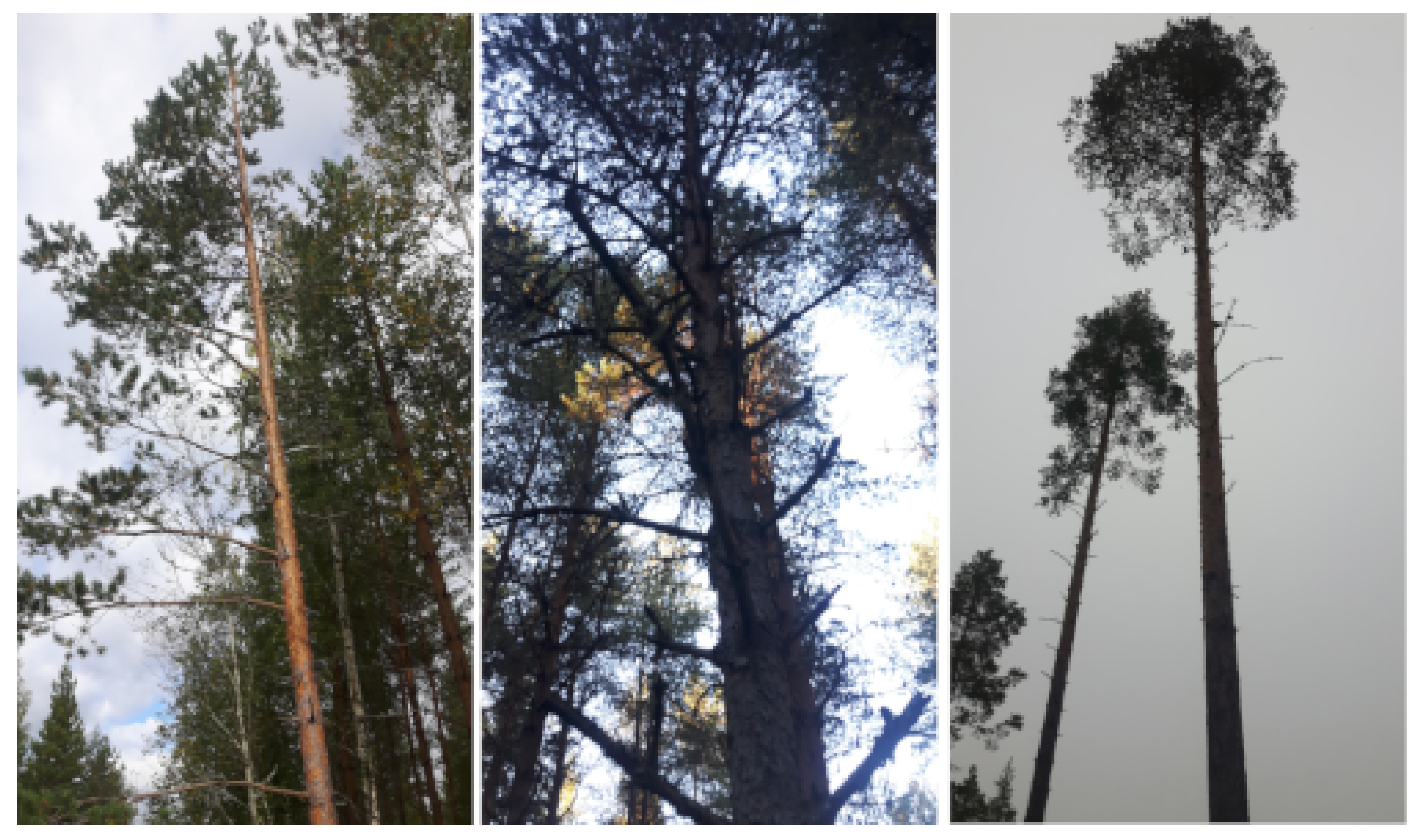
The samples were selected to represent both young and old forests, and trees with different amounts of branch densities (Figure 1). Trees 1–4 were located at a site with a stand age of 108 years and were a few of the remaining trees after harvesting. Stem density was 100 stems/ha. Trees 5–8 were located at a site with a stand age of 37 years. Stem density was 700 stems/ha. Trees 9 and 10 were located at a site with a stand age of 50 years and stem density of 800 stems/ha. Scots pine was selected since it is an important tree species in Scandinavian forestry.
The ten trees were first laser scanned and then felled. The height from the ground to the branch whorls was measured manually. The field sampled trees had a DBH of 19.2–38.5 cm and a tree height of 13.5–24.4 m, Table 1. The mean distances between branch whorls are 41 cm and the minimum and maximum distances between branch whorls are 10 cm and 120 cm, respectively. The branch diameters from the sample trees were in the range 0.24–9.27 cm.
2.2. Terrestrial Laser Scanning Data
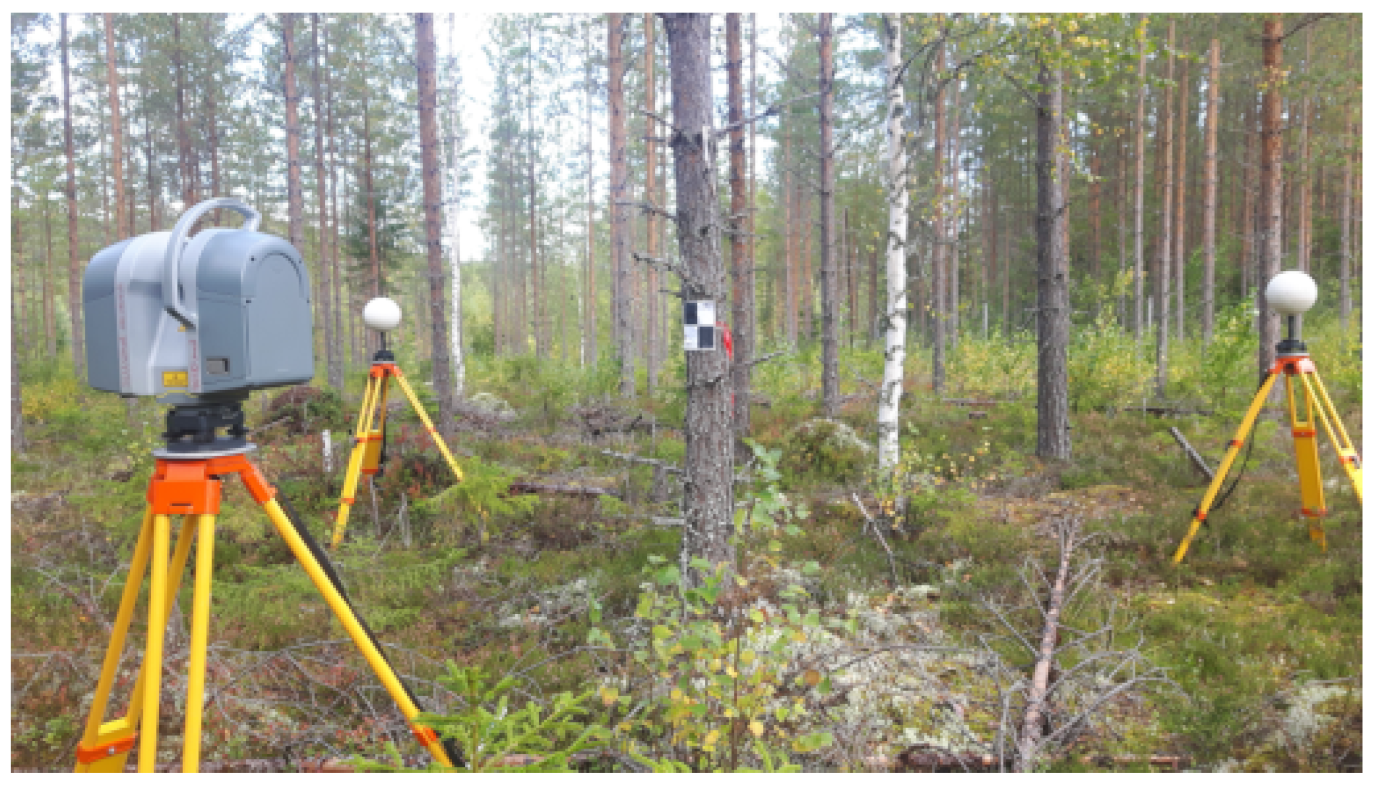
The ten trees were scanned with a terrestrial laser instrument, Trimble TX8, to obtain a detailed measurement of the stem and branches of each tree. The field of view was: 360° × 317°, beam divergence 0.34 mrad, 1 million laser points per second, and wavelength 1.5 μm (near-infra–red). One scan takes three minutes to complete. A multiscan setup was used with three instrument positions surrounding each tree. The first instrument position was set approximately 3 m south of the stem (180° azimuth). The other two instrument positions was set at 60° azimuth and 300° azimuth to cover all sides, both approximately 3 m from the stem. At each instrument position a tripod was placed. For every scan, one of the tripods had the TLS instrument fixed to it and the other two had white spherical targets attached to them. This was performed three times so that the TLS instrument scanned the trees from three directions. The TLS instrument had the zero coordinate at the center of the equipment, for each scan, so the spherical targets were used to co-register the data into a common coordinate system. The positions of the targets were detected in each of the scans in the TLS data. The three different datasets were then merged into one by using the detected coordinates of the targets. Trees were visible from all sides in the new merged point cloud data, Figure 2.
2.3. Branch Detection Algorithm
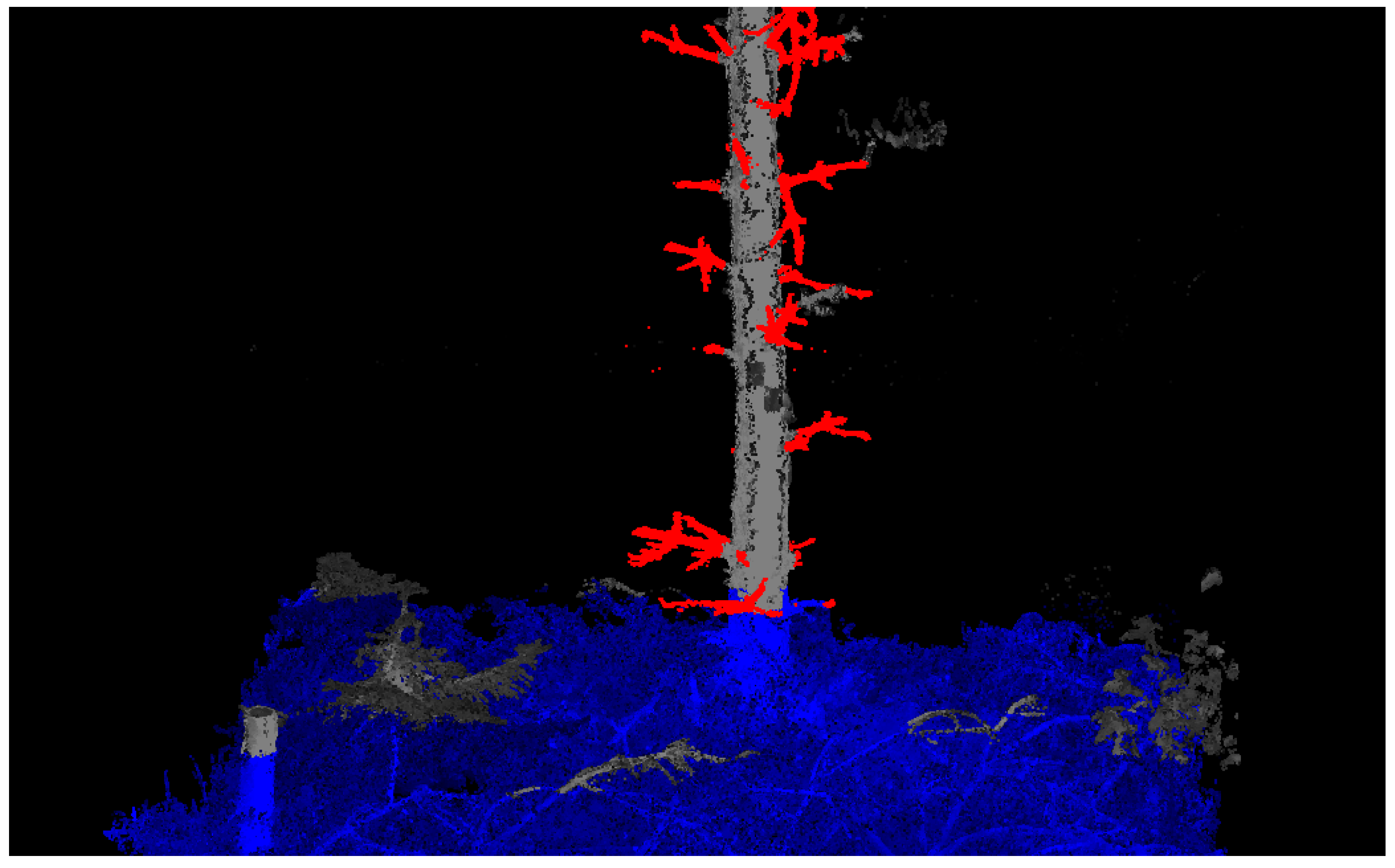
The outline of the branch attachment detection algorithm is as follows. The TLS data are saved in 3D-volume cells (voxels) of 3 cm size for easy access and data management. Voxels with fewer than 100 data points are not used. Stem profiles of the trees and ground models are detected using algorithms described in [21]. The output from the stem profile algorithms is a list of consecutive cylinders for each sample tree and by interpolating the cylinder list it is possible to achieve an estimated stem diameter at any height along the stem. After detecting the ground model and the stem profile models, the laser data can be classified into low vegetation points, near stem branch points, and unclassified points as a preprocessing step. The criteria for selecting classes is as follows. Data points that are closer than 50 cm from the height of the ground model are classified as low vegetation and not used. The remaining data points that are positioned within a radial distance interval from 5 cm to 50 cm from a stem are classified as near stem vegetation and kept for further processing, Figure 3.
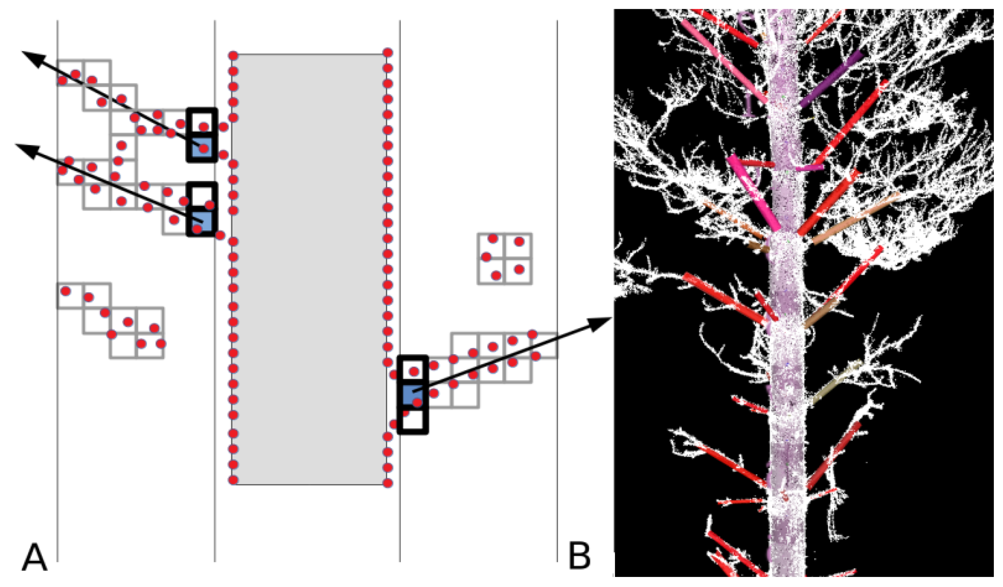
Only the data points that are classified as near stem points are used after the preprocessing step and saved in voxels. Filled near-stem voxels that are neighbors are clustered into groups, Figure 4A. These clusters are classified as possible branches. For each cluster, the voxels that have a radial distance from the stem profile that is less than 7 cm are classified as possible attachment points and kept for further processing. These attachment voxels are grouped into subclusters. Note that there can be more than one attachment subcluster per branch cluster but the most common is that each possible branch only has one attachment point. Several branches growing close together might sometimes be clustered as one big branch and would therefore have several attachment points. Arranging attachment points into subclusters is a way of finding each separate branch in cases like these. Clusters without attachment points are considered to be foliage or other noise and removed.
The voxel closest to the centroid in each attachment subcluster is chosen as the center position of the branch attachment, Figure 4A. From this position, a number of cylinder axes are tested in different directions. For each direction, the laser data points that are within a preselected radius of size 3 cm, from the current cylinder axis, are added to the voting for that particular direction. The votes for each direction are saved in a voting raster with coordinates u and v. To obtain an evenly distributed number of directions, the u and v coordinates are mapped to spherical coordinates using Equations (1).
where r is the radial distance, is the angle in radians from the z-axis, and is the angle in radians from the x-axis in the x–y plane. Equations (2) are used to map spherical to Cartesian coordinates.
where x, y, and z are the Cartesian coordinates.
The cylinder axis with the highest number of votes for each branch attachment, in the u–v voting raster, is selected as the center line of the selected cluster. The branch radius is modeled as the radial median of the data points to the center line of the selected cluster, Figure 4B.
2.4. Data Processing
The data processing was performed using software developed by the authors. The pre- and post-processing of the text-based data was performed using the Python scripting language. The algorithm for detecting stem profiles in TLS data and the new code for detecting branches in classified point cloud data were implemented using the C-programing language. Output from the stem profile and branch detection algorithms were saved in text files for post-processing and analysis. Stem profile detection of 15 m plots takes about 1–3 h to process depending on the stem density and average tree heights of the plot. Branch detection processing takes less than 5 min for one tree. An Intel Xeon E5-2690v4 2.6 GHz, 128 GB compute node was used for the main processing tasks. The Python script was used on various pieces of office PC equipment.
2.5. Evaluation
The height of every estimated branch cylinder from the TLS data was compared to the manually measured height of each branch whorl. If at least one estimated branch was positioned within an interval of ±10 cm from the manually measured whorl, it was considered to be a detected whorl. This interval was reduced if two consecutive manually measured branch whorls were positioned closer than the interval. If no TLS-estimated branch was found within this interval, it was set to be an omission error . TLS-estimated branches outside these intervals were set to be commission errors .
The accuracy of the algorithm was evaluated using the detection rate , Equation (3), the omission rate , Equation (4), and the commission rate , Equation (5)
where
- = number of whorls
- = number of detected whorls
- = number of undetected whorls (omission errors)
- = number of false whorls (commission errors).
The results were evaluated for each individual sample tree and for all trees. The number of detected whorls at the height interval of 0–10 m from the ground was also used and compared to the number of detected whorls at the full length of the trees, to see how well the algorithm works at the lower level.
3. Results
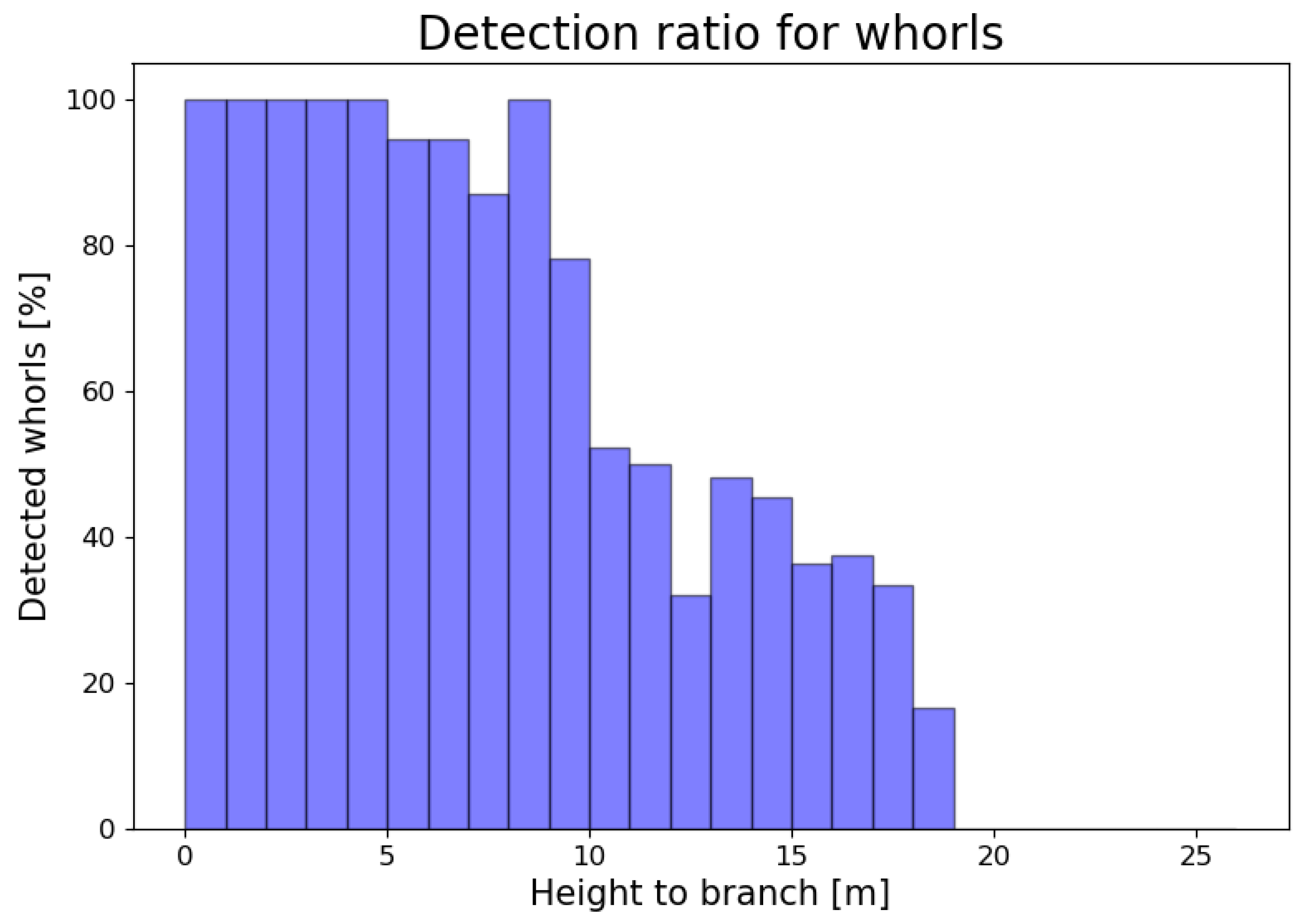
The comparison of the laser-detected branch whorls with the manually measured whorls show that the algorithm finds more than 90% of the branch whorls attached below 10 m from the ground, Figure 5, Table 2. Higher up, the detection rate diminishes, probably as a result of the lower branches covering the higher parts of the tree. In total, for all trees up to the top, 63.3% of the branch whorls were detected.
For the omission error rate, (Equation (4), Table 3), it can be seen that the different sample trees differ from 18.4 to 48.9% for the full length of the trees, and from 0.0 to 20.0% for the height interval 0–10 m. For the commission error rate (Equation 5, Table 3), it can be seen that the different sample trees differ from 5.0 to 46.4 for the full length of the trees and 0.0–44.4 for the height interval 0–10 m. For all trees, the omission error rate was 36.7% for the full height interval and 9.2% for the height interval 0–10 m. The commission error rate for all trees was 24.3% for the full height interval and 29.5% for the height interval 0–10 m, Table 3.
The fact that the commission error rate is higher at the height interval 0–10 m compared to the full height interval can be explained by the fact that most commission errors appear at the lower level of the trees. Correspondingly, the omission error rate is lower at the height interval 0–10 m compared to the full height interval, which can be explained by the fact that most omission errors appear at a higher level in the canopy where there is a high amount of shaded zones, and where the laser beams cannot penetrate.
All in all, the algorithm seems to work well at the lower level of the trees where there is not too much self-shading by branches. The lower branches occlude the higher branches if the instrument is positioned at the ground, making it difficult to detect detailed structures higher up. The detection rate at the lower level is high and makes it possible to discriminate most of the branch whorls.
4. Discussion
The research area of estimating tree architecture in TLS data is relatively new and there are not many studies that compare the results with data suitable for inventory applications in forestry. Many of the earlier papers concentrated on finding algorithms that were robust enough to be able to detect stems and branches in point cloud data. However, they did not evaluate the results with forestry parameters from the trees they measured. Most of them conducted a visual inspection of the results [5,6,7,8,9,18], whereas others compared the estimates from the algorithm with the data from artificial trees [11].
We only found five studies that compared to sampled forestry parameters from a ground truth. Dassot et al. [20], for instance, evaluated the total volumes of branches with a diameter larger than 7 cm of eight species in France and found that the accuracy was within ±30% for 31 out of 36 sample trees. Hackenberg et al. [16] conducted a linear regression analysis of the correlation between the ground truth and TLS-estimated data of volumes for 14 branches of four species in Germany and found an adjusted coefficient of determination of 0.96. Lau et al. [12] tested nine tropical trees of three species in central Guyana with branches in a diameter span of 10–20 cm and found a reconstruction accuracy of 45%, and that the diameters were overestimated by 40%. Pyörälä et al. [4] observed an overall accuracy of 68.6% for quantitative branch detection of 158 Scots pine trees with 2561 sampled branches with diameters > 0.7 cm. This result is similar to the 63% branch whorl detection rate in our study. Zhang et al. [13] found a relative root mean square error of 14.62% for branch lengths and 11.96% for branch numbers on ten sample trees.
There were some different techniques used in these five studies. The paper by Dassot et al. [20] describes a semi-automatic reconstruction process using polylines and circle fitting. Since their method is partly manual, it would not be considered in full-scale industrial solutions. However, in laboratory settings, the method should work well.
Hackenberg et al. [16] used spherical neighborhoods to find and model cylinders in point cloud data. Their method models junctions of the stems and receives a hierarchical tree structure, which later can be used as a model of the tree and branches.
Lau et al. [12] and Zhang et al. [13] used quantitative structural models that also give hierarchical tree structures. However, the method by Lau et al. [12] had a low detection rate on small branches. Zhang et al. [13] reached a better outcome with, for instance, a root mean square error of 11.96% for branch numbers.
The method by Pyörälä et al. [4] has the largest ground truth of these studies. Their techniques are based on searching in the neighborhood of a stem profile, like in our study, and their detection results are comparable to ours.
All these studies led to the development of the research field with many new methods and techniques. However, to take the research field further, there is a need to have more comparisons with ground truth data of different stem quality parameters of interest. This will give practitioners useful insights into what accuracies to expect from estimates of forestry parameters from TLS data.
In this study, we have presented a new algorithm for detecting branch attachments to stems that is based on a voxel approach and line object detection by a voting procedure. The method works well at the lower levels of the trees in pines of various ages and with different kinds of branch structures. At higher levels of the tree, however, the occluding effects of the branches block an efficient detection rate. A solution for detecting branches high in the canopy is needed. For instance, by using drones or elevated TLS equipment [22]. There is also a need to investigate other types of tree species, beginning with those common in forestry applications. One large difference would be when going from single-stem trees to trees where there are many stems and large branches that separate early. In that case, another stem detection algorithm would be necessary. The current stem profile detection algorithm was evaluated on spruces and pines [21], and gave a root mean square error of 1.104 cm and an omission error of 10.2% when detecting stem diameters at different heights of the trees.
There are a number of scenarios where the system presented in this study could be applied in the future. For instance, the branch density of each standing tree could be used to evaluate the quality of stems. Taper sweep and lean of the stems could also be estimated if this method is combined with, for instance, the stem profile detection algorithm presented by Olofsson and Holmgren [21]. The information of branch angles could also be used as input to tree species classification algorithms.
These techniques could also be part of large-scale inventory systems. For instance, laser measurement equipment could be attached to a harvester and connected to a computer to be used when selecting and planning the felling and cutting of trees. The stem information retrieved from this system could be used to train airborne laser scanning systems to build forest maps with quality data. The branch knot distribution is also an important indicator for the selection of wood quality class when crosscutting the logs on site.
Laser measurement systems could also be attached to terrain vehicles, backpacks, or tripods in order to do an inventory of the quality class of the trees in a stand. The trees detected at the field plot inventories can then be linked to trees detected from airborne systems as suggested by Olofsson and Holmgren [23]. Statistics from the laser data point clouds of the detected trees in the airborne systems that are linked to trees from the ground truth with a known quality can then be used as training data. By choosing variables with high correlation to the attributes of choice, models can be built that can produce forest quality stem maps that cover large regions.
For future studies, it is important to test how well the algorithms work on laser data from different types of sensors, for instance mobile or backpack-carried systems. It is also of interest to investigate how well the algorithms detect branches in other types of tree species. It would also be of interest to use full 3D models of the stem, branches, twigs, and foliage. For instance, modeled by Côté et al. [8] for the purpose of assessing stem quality on forest stands and thereby giving data to forest operation planning systems.
Author Contributions
Conceptualization, K.O. and J.H.; methodology, K.O.; software, K.O.; validation, K.O.; formal analysis, K.O.; investigation, K.O.; resources, J.H.; data curation, J.H.; writing—original draft preparation, K.O.; writing—review and editing, J.H.; project administration, J.H.; funding acquisition, J.H. All authors have read and agreed to the published version of the manuscript.
Funding
This study was financed by the K E Önnesjö Foundation, the Nils & Dorthi Troëdsson Foundation, the Bo Rydin Foundation for Scientific Research, the Mistra Digital Forest Program, the Tandem Forest Value Program, and the Swedish Foundation for Strategic Research.
Data Availability Statement
Data sharing is not applicable to this paper.
Acknowledgments
We would like to thank Ola Langvall and the Unit for Field-Based Forest Research for data collection at the Siljansfors research park.
Conflicts of Interest
The authors declare no conflict of interest.
References
- Holopainen, M.; Vastaranta, M.; Hyyppä, J. Outlook for the Next Generation’s Precision Forestry in Finland. Forests 2014, 5, 1682–1694. [Google Scholar] [CrossRef] [Green Version]
- Hyyppä, J.; Hyyppä, H.; Leckie, D.; Gougeon, F.; Yu, X.; Maltamo, M. Review of methods of small–footprint airborne laser scanning for extracting forest inventory data in boreal forests. Int. J. Remote Sens. 2008, 29, 1339–1366. [Google Scholar] [CrossRef]
- Liang, X.; Kankare, V.; Hyyppä, J.; Wang, Y.; Kukko, A.; Haggrén, H.; Yu, X.; Kaartinen, H.; Jaakkola, A.; Guan, F.; et al. Terrestrial laser scanning in forest inventories. ISPRS J. Photogramm. Remote Sens. 2016, 115, 63–77. [Google Scholar] [CrossRef]
- Pyörälä, J.; Liang, X.; Saarinen, N.; Kankare, V.; Wang, Y.; Holopainen, M.; Hyyppä, J.; Vastaranta, M. Assessing branching structure for biomass and wood quality estimation using terrestrial laser scanning point clouds. Can. J. Remote Sens. 2018, 44, 462–475. [Google Scholar] [CrossRef] [Green Version]
- Gorte, B.; Pfeifer, N. Structuring laser-scanned trees using 3D mathematical morphology. Int. Arch. Photogramm. Remote Sens. 2004, 35, 929–933. [Google Scholar]
- Cheng, Z.L.; Zhang, X.P.; Chen, B.Q. Reconstruction of Tree Branches from a Single Range Image. J. Comput. Sci. Technol. 2007, 22, 846–848. [Google Scholar] [CrossRef]
- Bucksch, A.; Lindenbergh, R. CAMPINO—A skeletonization method for point cloud processing. ISPRS J. Photogramm. Remote Sens. 2008, 63, 115–127. [Google Scholar] [CrossRef]
- Côté, J.F.; Widlowski, J.L.; Fournier, R.A.; Verstraete, M.M. The structural and radiative consistency of three-dimensional tree reconstructions from terrestrial lidar. Remote Sens. Environ. 2009, 113, 1067–1081. [Google Scholar] [CrossRef]
- Ai, M.; Yao, Q.; Wang, Y.; Wei, W. An Automatic Tree Skeleton Extraction Approach Based on Multi-View Slicing Using Terrestrial LiDAR Scans Data. Remote Sens. 2020, 12, 3824. [Google Scholar] [CrossRef]
- Chaudhury, A.; Godin, C. Skeletonization of Plant Point Cloud Data Using Stochastic Optimization Framework. Front. Plant Sci. 2020, 11, 773. [Google Scholar] [CrossRef]
- Raumonen, P.; Kaasalainen, M.; Åkerblom, M.; Kaasalainen, S.; Kaartinen, H.; Vastaranta, M.; Holopainen, M.; Disney, M.; Lewis, P. Fast Automatic Precision Tree Models from Terrestrial Laser Scanner Data. Remote Sens. 2013, 5, 491–520. [Google Scholar] [CrossRef] [Green Version]
- Lau, A.; Patrick Bentley, L.; Martius, C.; Shenkin, A.; Harm, B.; Raumonen, P.; Malhi, Y.; Jackson, T.; Herold, M. Quantifying branch architecture of tropical trees using terrestrial LiDAR and 3D modelling. Trees 2018, 32, 1219–1231. [Google Scholar] [CrossRef] [Green Version]
- Zhang, C.; Yang, G.; Jiang, Y.; Xu, B.; Li, X.; Zhu, Y.; Lei, L.; Chen, R.; Dong, Z.; Yang, H. Apple Tree Branch Information Extraction from Terrestrial Laser Scanning and Backpack-LiDAR. Remote Sens. 2020, 12, 3592. [Google Scholar] [CrossRef]
- Bremer, M.; Rutzinger, M.; Wichmann, V. Derivation of tree skeletons and error assessment using LiDAR point cloud data of varying quality. ISPRS J. Photogramm. Remote Sens. 2013, 80, 39–50. [Google Scholar] [CrossRef]
- Li, Y.; Su, Y.; Zhao, X.; Yang, M.; Hu, T.; Zhang, J.; Liu, J.; Liu, M.; Guo, Q. Retrieval of tree branch arhitecture attributes from terrestrial laser scan data using a Laplacian algorithm. Agric. For. Metrol. 2020, 284, 107874. [Google Scholar] [CrossRef]
- Hackenberg, J.; Morhart, C.; Sheppard, J.; Spiecker, H.; Disney, M. Highly Accurate Tree Models Derived from Terrestrial Laser Scan Data: A Method Description. Forests 2014, 5, 1069–1105. [Google Scholar] [CrossRef] [Green Version]
- Xi, Z.; Hopkinson, C.; Chasmer, L. Filtering Stems and Branches from Terrestrial Laser Scanning Point Clouds Using Deep 3D Fully Convolutional Networks. Remote Sens. 2018, 10, 1215. [Google Scholar] [CrossRef] [Green Version]
- Eysn, L.; Pfeifer, N.; Ressl, C.; Hollaus, M.; Grafl, A.; Morsdorf, F. A Practical Approach for Extracting Tree Models in Forest Environments Based on Equirectangular Projections of Terrestrial Laser Scans. Remote Sens. 2013, 5, 5424–5448. [Google Scholar] [CrossRef] [Green Version]
- Pyörälä, J.; Kankare, V.; Vastaranta, M.; Rikala, J.; Holopainen, M.; Sipi, M.; Hyyppä, J.; Uusitalo, J. Comparison of terrestrial laser scanning in measuring Scots Pine (Pinus sylvestris L.) branch structure. Scand. J. For. Res. 2018, 33, 291–298. [Google Scholar] [CrossRef] [Green Version]
- Dassot, M.; Colin, A.; Santenoise, P.; Fournier, M.; Constant, T. Terrestrial laser scanning for measuring the solid wood volume, including branches of adult standing treess in the forest environment. Comput. Electron. Agric. 2012, 89, 86–93. [Google Scholar] [CrossRef]
- Olofsson, K.; Holmgren, J. Single Tree Stem Profile Detection Using Terrestrial Laser Scanner Data, Flatness Saliency Features and Curvature Properties. Forests 2016, 7, 207. [Google Scholar] [CrossRef]
- Rocha, K.D.; Silva, C.A.; Cosenza, D.N.; Mohan, M.; Klauberg, C.; Schlickmann, M.B.; Xia, J.; Leite, R.V.; Alves de Almeida, D.R.; Atkins, J.W.; et al. Crown-Level Structure and Fuel Load Characterization from Airborne and Terrestrial Laser Scanning in a Longleaf Pine (Pinus palustris Mill.) Forest Ecosystem. Remote Sens. 2023, 15, 1002. [Google Scholar] [CrossRef]
- Olofsson, K.; Holmgren, J. Co-registration of single tree maps and data captured by a moving sensor using stem diameter weighted linking. Silva Fenn. 2022, 56, 10712. [Google Scholar] [CrossRef]
Figure 1.
Examples of young and old sample trees with different branching patterns. (Left) Pine tree from a stand of age 37 years. (Middle) Pine from a stand of age 50 years, with thick branches from ground to tree top. (Right) Pines from a stand of age 108 years. A large part of the stems only have small branches. The tree crowns at the top have thicker branches.

Figure 2.
Terrestrial laser scanner experimental setup. The white spheres are targets used when co-registering laser datasets from different scan angles. The black and white sheet on the tree is a target used when co-registering laser data and manually sampled data.
Figure 2.
Terrestrial laser scanner experimental setup. The white spheres are targets used when co-registering laser datasets from different scan angles. The black and white sheet on the tree is a target used when co-registering laser data and manually sampled data.

Figure 3.
Preprocessing of pointcloud. Ground vegetation class in blue, near stem branches class in red, and unclassified points in gray.
Figure 3.
Preprocessing of pointcloud. Ground vegetation class in blue, near stem branches class in red, and unclassified points in gray.

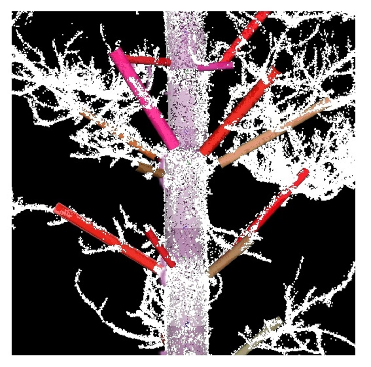
Figure 4.
(A) Sketch of the branch detection algorithm. Laser data as red dots, stem profile as a large grey rectangle, near stem zone marked with thin lines, 3D cluster cells as small squares, stem attachment cells as black squares, selected start cell for branch detection in blue, estimated stem axes as arrows. (B) Estimated branch attachments to pine in the field data were measured with a terrestrial laser scanner. White dots are laser data. Red cylinders are the branch attachment estimates. The weakly colored cylinders are the stem profile estimate.

Figure 5.
Detection rate of the branch whorls as a function of height from ground. Most of the branch whorls are detected up to a 10 m height from the ground.
Figure 5.
Detection rate of the branch whorls as a function of height from ground. Most of the branch whorls are detected up to a 10 m height from the ground.


Table 1.
Field-sampled trees used in the study. DBH is the stem diameter at breast height.
| Tree | DBH [cm] | Height [m] | Height to First Green Branch [m] |
|---|---|---|---|
| 1 | 27.3 | 21.9 | 13.0 |
| 2 | 32.0 | 21.0 | 12.4 |
| 3 | 38.5 | 24.4 | 11.4 |
| 4 | 29.2 | 21.8 | 14.1 |
| 5 | 20.9 | 14.9 | 5.9 |
| 6 | 22.9 | 15.7 | 4.8 |
| 7 | 19.2 | 13.5 | 4.9 |
| 8 | 21.4 | 14.4 | 2.6 |
| 9 | 20.0 | 16.5 | 6.5 |
| 10 | 30.4 | 20.8 | 11.2 |
Table 2.
Amount of detected whorls in terrestrial laser scanner data for each sample tree, for all trees, and for all trees at the height interval 0–10 m from the ground.
Table 2.
Amount of detected whorls in terrestrial laser scanner data for each sample tree, for all trees, and for all trees at the height interval 0–10 m from the ground.
| Tree | Detected Whorls | All Whorls | Detection Rate [%] |
|---|---|---|---|
| 1 | 28 | 39 | 71.8 |
| 2 | 23 | 41 | 56.1 |
| 3 | 24 | 31 | 77.4 |
| 4 | 31 | 38 | 81.6 |
| 5 | 15 | 26 | 57.7 |
| 6 | 15 | 28 | 53.6 |
| 7 | 19 | 31 | 61.3 |
| 8 | 18 | 28 | 64.3 |
| 9 | 24 | 40 | 60.0 |
| 10 | 24 | 47 | 51.1 |
| all trees | 221 | 349 | 63.3 |
| all trees (branches < 10 m from ground) | 148 | 163 | 90.8 |
Table 3.
Omission and commission error rates (Equations (4) and (5)) for each sample tree and for all trees, both for all branch whorls and for branch whorls at a height interval of 0–10 m from the ground.
| Tree | [%] | (0–10 m) [%] | [%] | (0–10 m) [%] |
|---|---|---|---|---|
| 1 | 12.5 | 14.3 | 28.2 | 7.7 |
| 2 | 25.8 | 42.9 | 43.9 | 20.0 |
| 3 | 20.0 | 33.3 | 22.6 | 11.1 |
| 4 | 6.1 | 0.0 | 18.4 | 18.2 |
| 5 | 21.1 | 22.2 | 42.3 | 6.7 |
| 6 | 46.4 | 44.4 | 46.4 | 11.8 |
| 7 | 5.0 | 5.0 | 38.7 | 17.4 |
| 8 | 40.0 | 40.0 | 35.7 | 5.3 |
| 9 | 31.4 | 31.4 | 40.0 | 4.0 |
| 10 | 29.4 | 32.3 | 48.9 | 0.0 |
| all | 24.3 | 29.5 | 36.7 | 9.2 |
Disclaimer/Publisher’s Note: The statements, opinions and data contained in all publications are solely those of the individual author(s) and contributor(s) and not of MDPI and/or the editor(s). MDPI and/or the editor(s) disclaim responsibility for any injury to people or property resulting from any ideas, methods, instructions or products referred to in the content. |
© 2023 by the authors. Licensee MDPI, Basel, Switzerland. This article is an open access article distributed under the terms and conditions of the Creative Commons Attribution (CC BY) license (https://creativecommons.org/licenses/by/4.0/).
Share and Cite
MDPI and ACS Style
Olofsson, K.; Holmgren, J. Stem Quality Estimates Using Terrestrial Laser Scanning Voxelized Data and a Voting-Based Branch Detection Algorithm. Remote Sens. 2023, 15, 2082. https://doi.org/10.3390/rs15082082
AMA Style
Olofsson K, Holmgren J. Stem Quality Estimates Using Terrestrial Laser Scanning Voxelized Data and a Voting-Based Branch Detection Algorithm. Remote Sensing. 2023; 15(8):2082. https://doi.org/10.3390/rs15082082
Chicago/Turabian StyleOlofsson, Kenneth, and Johan Holmgren. 2023. "Stem Quality Estimates Using Terrestrial Laser Scanning Voxelized Data and a Voting-Based Branch Detection Algorithm" Remote Sensing 15, no. 8: 2082. https://doi.org/10.3390/rs15082082
Note that from the first issue of 2016, this journal uses article numbers instead of page numbers. See further details here.