Underground Water Level Prediction in Remote Sensing Images Using Improved Hydro Index Value with Ensemble Classifier

Abstract

The economic sustainability of aquifers across the world relies on accurate and rapid estimates of groundwater storage changes, but this becomes difficult due to the absence of in-situ groundwater surveys in most areas. By closing the water balance, hydrologic remote sensing measures offer a possible method for quantifying changes in groundwater storage. However, it is uncertain to what extent remote sensing data can provide an accurate assessment of these changes. Therefore, a new framework is implemented in this work for predicting the underground water level using remote sensing images. Generally, the water level is defined into five levels: Critical, Overexploited, Safe, Saline, and Semi-critical, based on water quantity. In this manuscript, the remote sensing images were acquired from remote sensing images. At first, Wiener filtering was employed for preprocessing. Secondly, the Vegetation Indexes (VI) (Normalized Difference Vegetation Index (NDVI), Normalized Difference Snow Index (NDSI), Infrared index (IRI), Radar Vegetation Index (RVI)), and statistical features (entropy, Root Mean Square (RMS), Skewness, and Kurtosis) were extracted from the preprocessed remote sensing images. Then, the extracted features were combined as a novel hydro index, which was fed to the Ensemble Classifier (EC): Neural Networks (NN), Support Vector Machine (SVM), and improved Deep Convolutional Neural Network (DCNN) models for underground water level prediction in the remote sensing images. The obtained results prove the efficacy of the proposed framework by using different performance measures. The results shows that the False Positive Rate (FPR) of the proposed EC model is 0.0083, which is better than that of existing methods. On the other hand, the proposed EC model has a high accuracy of 0.90, which is superior to the existing traditional models: Long Short-Term Memory (LSTM) network, Naïve Bayes (NB), Random Forest (RF), Recurrent Neural Network (RNN), and Bidirectional Gated Recurrent Unit (Bi-GRU).

1. Introduction

The groundwater is the world’s greatest supply of fresh water, and it is crucial for human consumption and general development of an area [1,2,3]. The water food energy nexus is mostly dependent on groundwater, which accounts for close to 30% of the world’s freshwater reserves [4,5,6]. Globally, groundwater supplies provide nearly half of the world’s drinking water. In addition, groundwater is widely utilized in agricultural processes, and demand is rising as a result of population growth, dietary changes, and climate change [7,8,9]. In order to measure aquifer degradation and to provide key data for developing a groundwater model to manage the resource, monitoring of groundwater withdrawal (pumping) is required [10,11,12]. Groundwater can reliably supply the necessary amount of high-quality water; therefore, effective water conservation plans are crucial for the long-term use of groundwater. Excessive groundwater extraction and improper aquifer recharging are two major factors in the depletion of groundwater in many regions. To promote effective use and organized management of groundwater resources, precise estimation and prediction of groundwater recharge should be carried out. This makes groundwater potential mapping with the use of yield data crucial. Data on yields include extraction volume and groundwater velocity at several measurement locations. Groundwater yield is influenced by local geological, topographic, and human-made factors, which are connected to groundwater potential [13,14]. The conventional methods in use to calculate groundwater pumping rely on predictions of agricultural water demand, which are generally made using the evapotranspiration and soil model, and surface water availability [15]. Remote sensing and Geographic Information Systems (GIS) present novel chances for hydrogeological research [16,17]. Maps that show the presence of groundwater are deployed to determine the geology, soil, geomorphology flow depth, rainfall, and land use [18]. Understanding that groundwater (shallow) flow is often influenced by precise surface force and characterized by geologic characteristics that may be deduced from surface data is essential to remotely sensing the water in the ground [19]. Topographic driving factors are a need for the conceived groundwater flow system at various sizes. Since remote sensing offers additional opportunities for groundwater detection, it will be much more successful in estimating water flows in the local ground than the topographically driven flow model. The contributions of this paper are specified below:

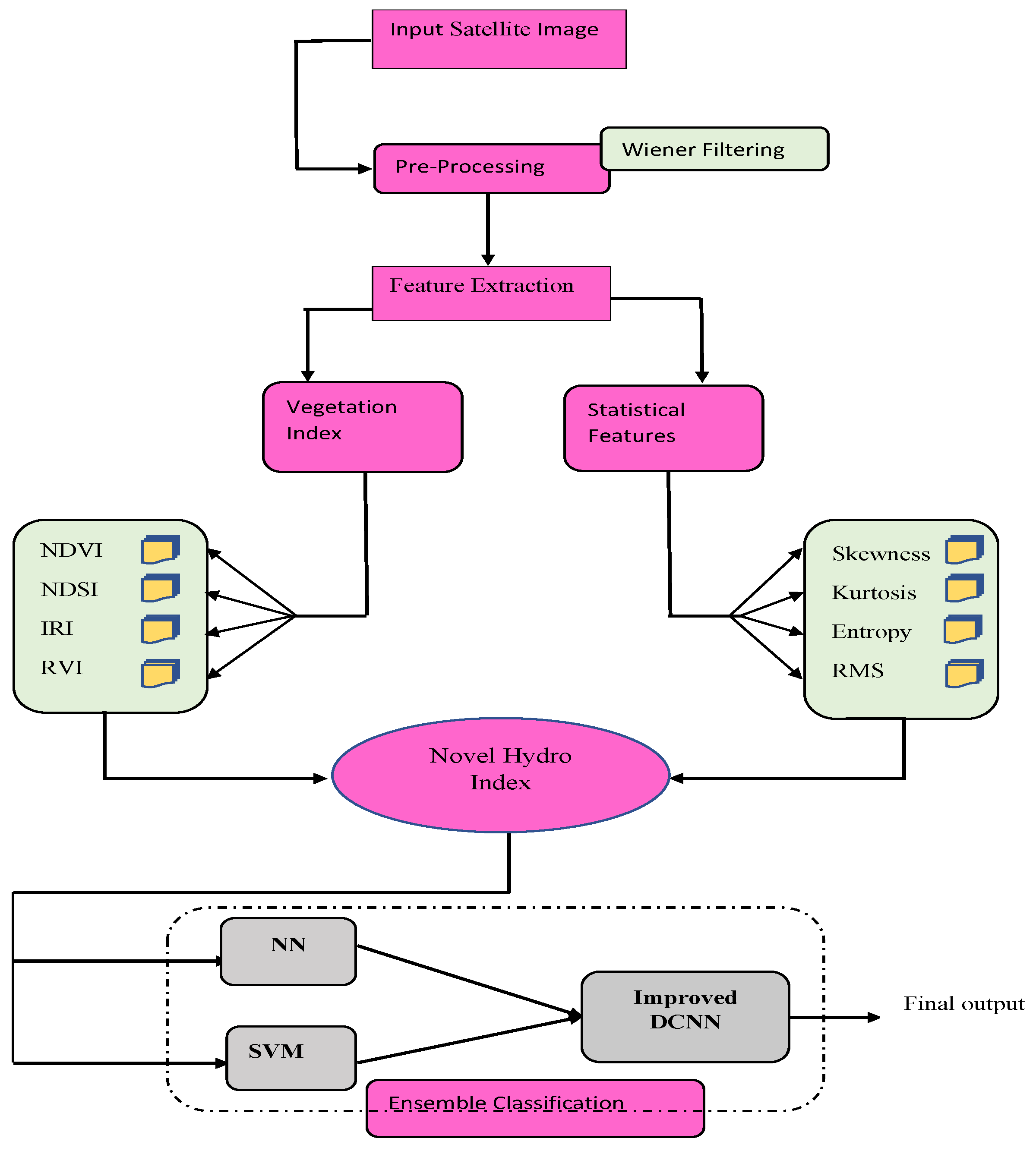
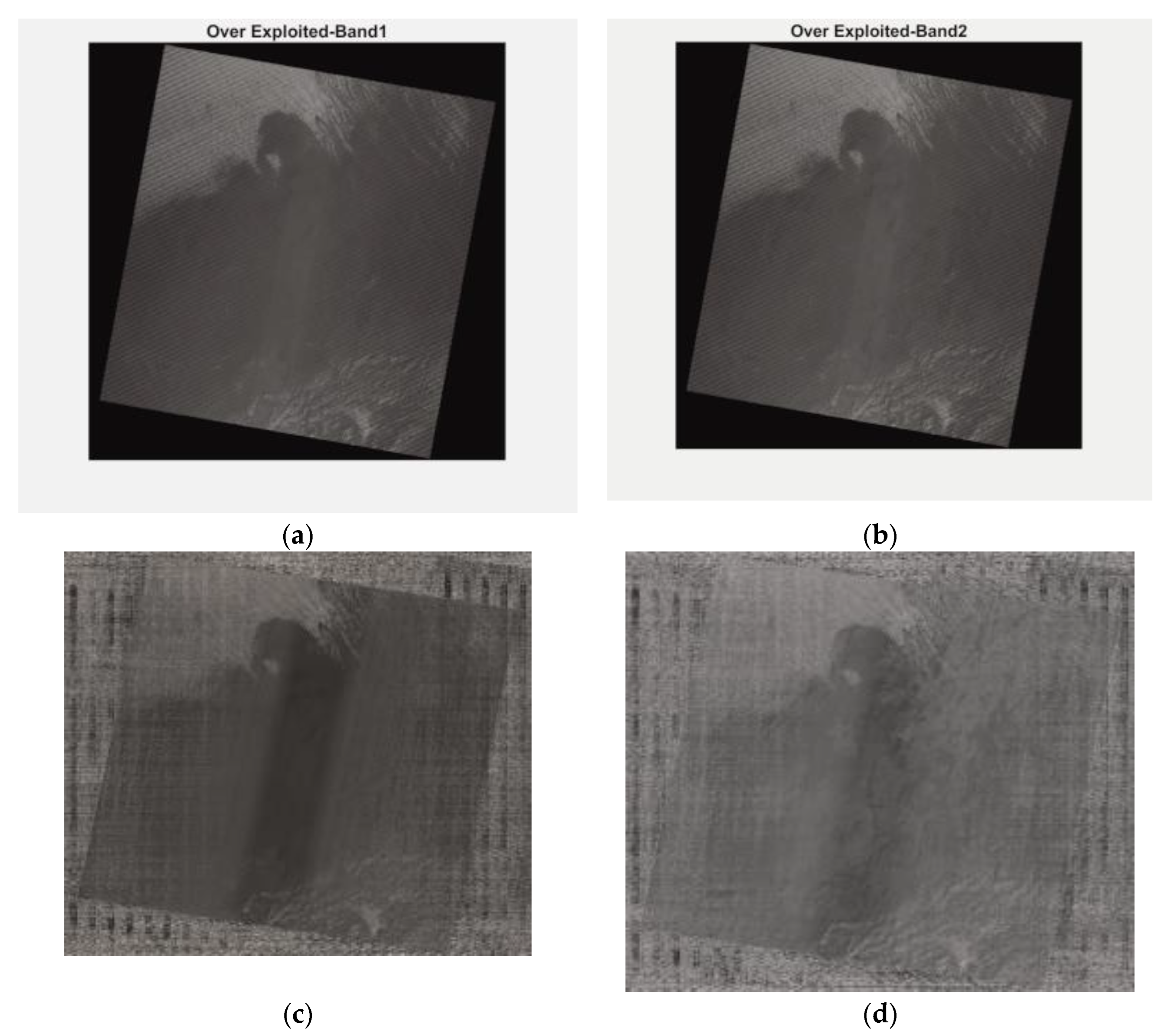
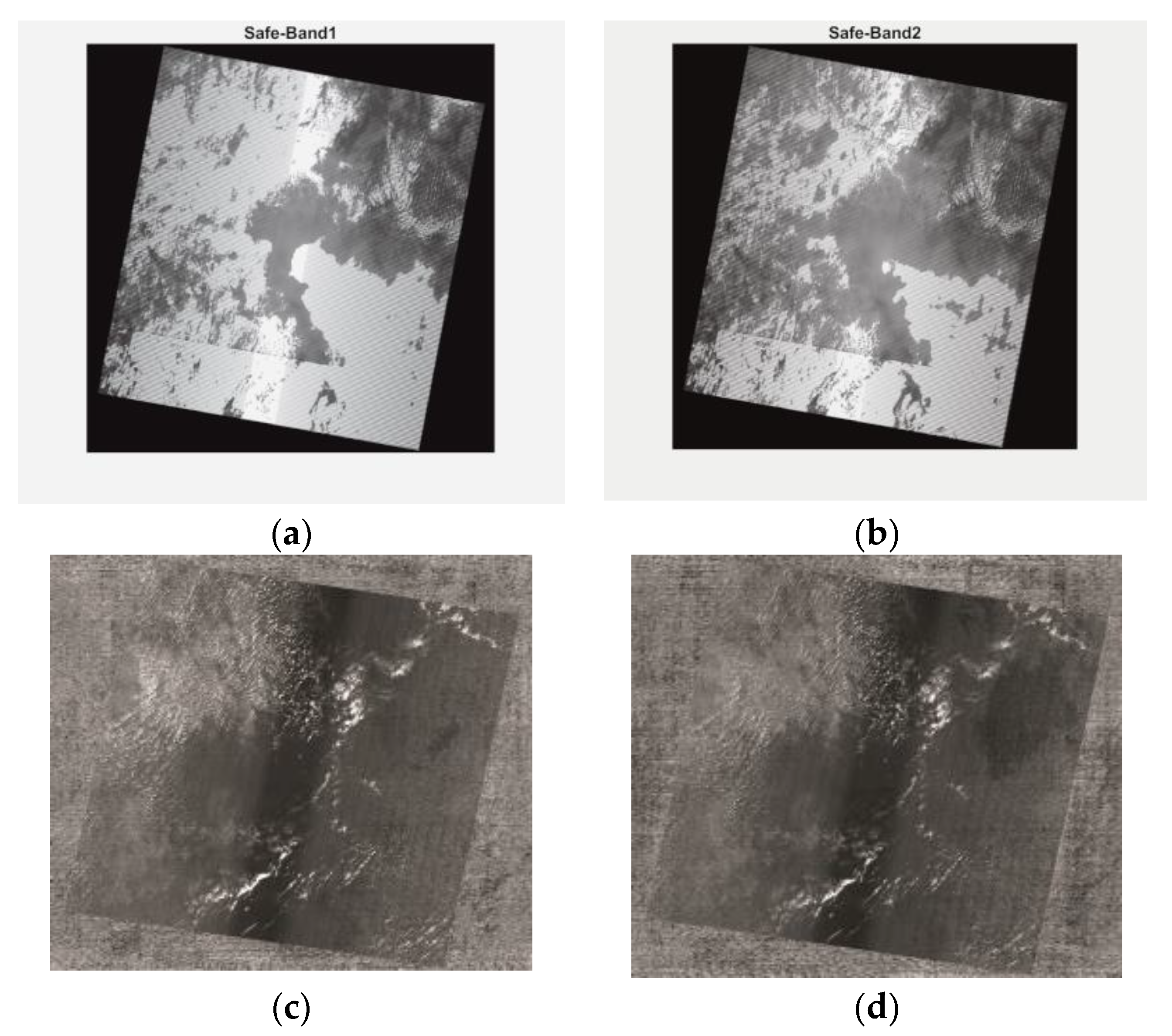
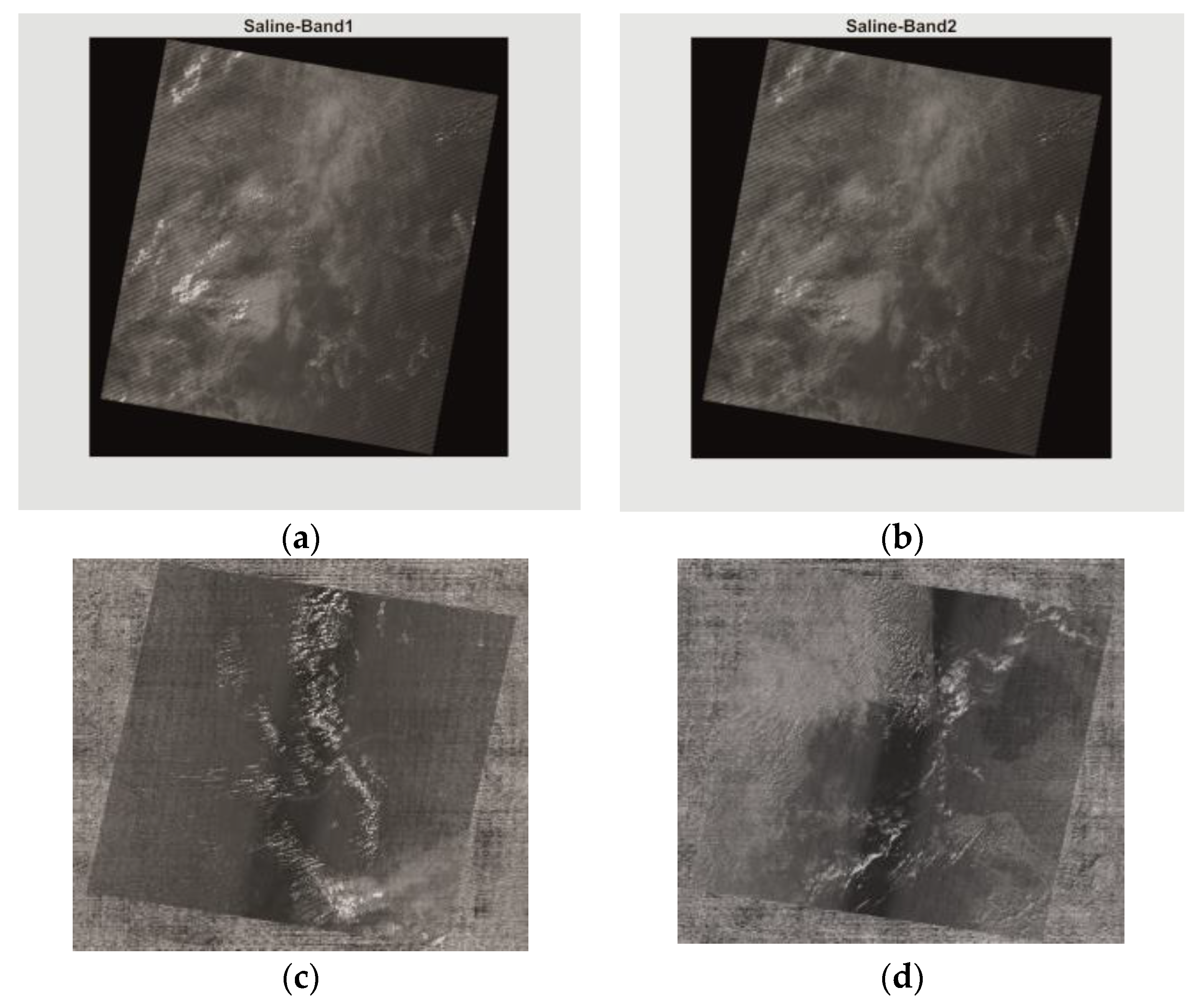
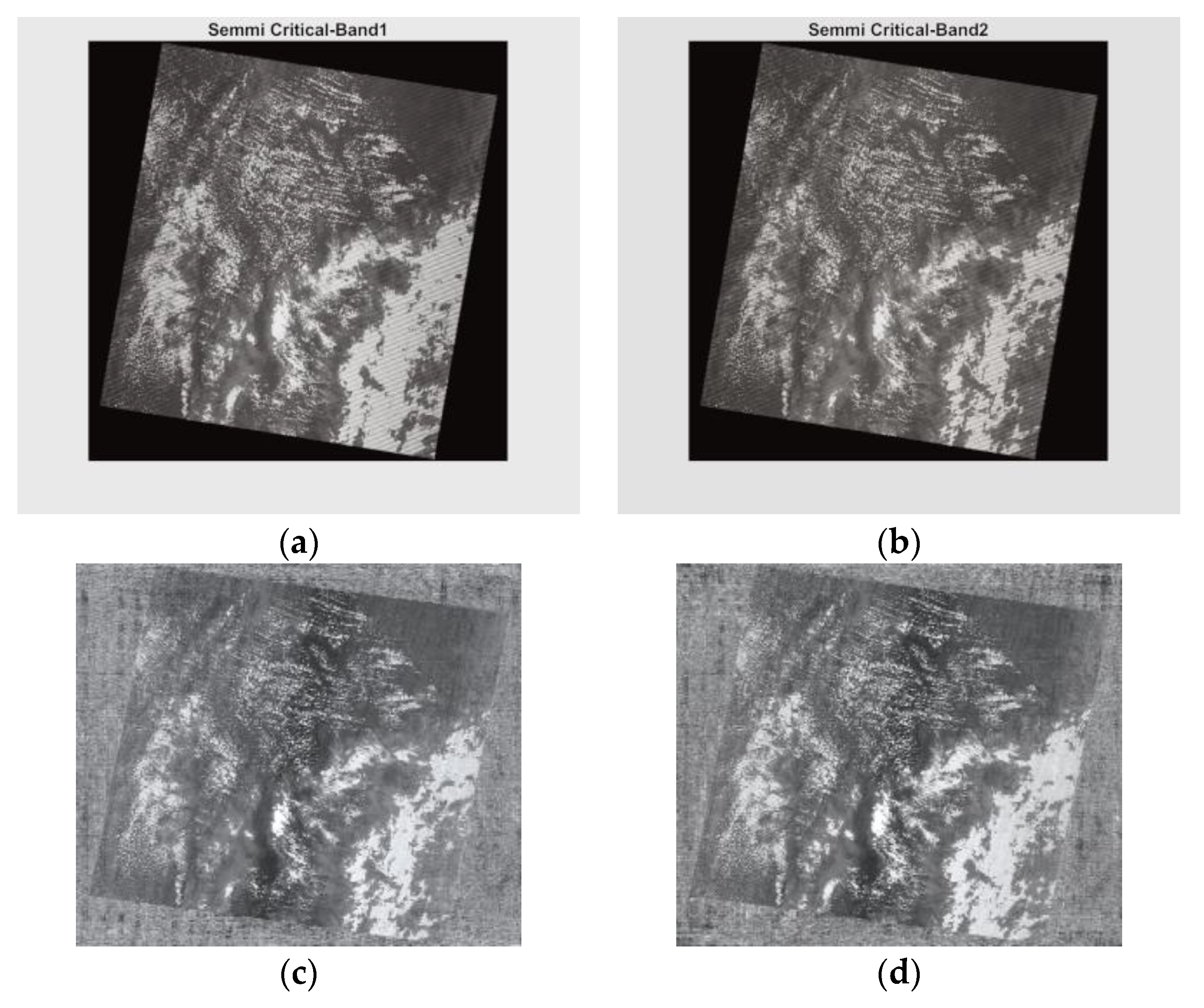
• Developed a Wiener filter for inverting the blurring and eliminating the additive noise from the acquired remote sensing images. In addition, the Wiener filter is optimal by minimizing the overall mean square error in the process of noise smoothing and inverse filtering;
• Integrated VI, NDVI, NDSI, IRI, and RVI, and statistical features for feature extraction. The extracted features are discriminative in that they decrease the sematic space between the feature subsets that help in improving the performance of underground water level prediction using remote sensing images;
• Proposed an EC model that includes improved NN, SVM, and DCNN for effective underground water level prediction.

The structure of this research is as follows; Section 2 explains existing works on the topic of underground water level prediction; Section 3 explains the concept of feature extraction and ensemble classification. The results and discussions are described in Section 4, and finally, the conclusion is stated in Section 5.

2. Literature Review

Majumdar et al. [20] developed a new strategy for groundwater level prediction that incorporates elements of the water balance with a Machine Learning (ML) algorithm. Here, the sensor data were used, which assessed various aspects of water balancing and land usage at various geographical resolutions, sequential resolutions, and multi-temporal satellite data. Evapotranspiration, moisture, and land cover were some of the remote sensing products. A cutting-edge ML approach, RF, was utilized to overcome these restrictions since combining these sets of data and then connecting them to groundwater flows utilizing physical models were inherently difficult processes. On both the training and testing datasets, the developed model withdrawals had a high level of accuracy. Veluguri et al. [21] planned to add unique hydro indicators that had not yet gained popularity in earlier methodologies. The developed work estimates statistical properties. In addition, VI incorporated “IRI transformation, Kath Thomas Tasseled cap transformation, normalized difference vegetation index, and simple ratio and the statistical and vegetation index were combined to create a unique hydro index”. Then, the ensemble method was used for an identification procedure that includes Deep Belief Network (DBN), NN, RF, and SVM. DBN produces the anticipated outcome by concerning certain metrics; the performance of the developed model was effective in comparison to prior models.

Zhengyang et al. [22] investigated the possibility of groundwater remote sensing in the framework of operational and future satellite-based sensors. The best use of remotely sensed data was integrated with ground-based data for GIS and numerical modeling. Further, to properly and effectively support product design and implementation in the mining region, Suganthi et al. [23] conducted research on feature information extraction. The analysis of Hyperspectral Remote Sensing Image (HRSI) technology’s detecting capabilities came first. HRSI has several bands and a high spectral resolution. As appropriate, certain bands can be removed to emphasize desired qualities. The spatial and spectral information was fully exploited in accordance with the features of HRSIs and the CNN depending upon Deep Learning (DL) was utilized for extracting the features. On training the features, CNN enables the computer to automatically extract data features.

Hai et al. set out to clearly explain the extant ML schemes used for modeling Groundwater Level (GWL) and milestones attained in this field [24]. Additionally, suggestions for potential upcoming research topics to increase the precision of GWL forecasts and broaden the field’s understanding were provided. For mapping potential areas of underground water in the western desert of Iraq, Mezheret al. [25] utilized statistical methods including Evidential Belief Function (EBF) and Logistic Regression (LR). The geographical interaction between groundwater wells and other conditioning elements was used to evaluate the potential of the groundwater regions. The thematic maps produced in this study demonstrated the efficacy of EBF and LR approaches for mapping groundwater potential.

To forecast GWL underneath ecosystems in the United States of America, Melissa et al. [26] employed satellite-based remote sensing. Groundwater decreases more commonly inside Groundwater Dependent Ecosystems (GDEs) located in regions of the state wherein groundwater resource management is lacking. Groundwater losses are most frequent within the GDEs located in those regions where sustained groundwater control is lacking. Shaimaa et al. [27] has offered two pumping scenarios. In the first scenario, it was assumed that over the next 50 years, the existing extraction rates would not change. The effectiveness of the aquifer was reciprocally influenced by geological and human factors. Nevertheless, despite its undeniable significance, groundwater levels in the utilization of water resources are frequently variable and rely on recharge from precipitation infiltration [28].

3. Methods

The steps involved in the proposed underground water level prediction framework are as follows: initially, the Wiener filter was utilized for image preprocessing. Then, the VI indexes (NDVI, NDSI, IRI, and RVI) and statistical features (entropy, RMS, Skewness, and Kurtosis) were used for feature extraction. Finally, an EC model (NN, SVM, and improved DCNN) was used for underground water level prediction. The illustrative depiction of the developed underground water level prediction model is represented in Figure 1.

3.1. Preprocessing

The input image $I\left(n,m\right)$ is subjected to a process under Wiener filtering, which aims to calculate a statistical estimate of an unknown image by employing a similar image as an input and filtering that known image to create the estimate as an output. In the Weiner filter, both the blurring and the gaussian type additive noises are instantly reversed. In the process of inverse filtering and noise smoothing, it minimizes the total mean square error so that the Wiener filter can offer the best mean square error performances. The attained preprocessed image is then passed to the next stage for extracting features. It is mathematically defined as the $I\left(n,m\right)$ which takes the Discrete Fourier Transform (DFT) to obtain $A\left(u,v\right)$. The original spectrum is estimated by taking the product of $A\left(u,v\right)$ and $G\left(u,v\right)$. The Wiener filter $G\left(u,v\right)$ is in Equation (1), where $H\left(u,v\right)$ is the Fourier transform of the point spread function, and $P_s\left(u,v\right)$ is the power spectrum of the signal process, and $P_n\left(u,v\right)$ of the noise process.

$$G\left(u,v\right)=\frac{H^{\ast }\left(u,v\right)P_s\left(u,v\right)}{{\left|H\left(u,v\right)\right|}^2{P}_s\left(u,v\right)+P_n\left(u,v\right)}$$

(1)

Here, DFT is applied in a long-time series of satellite images (data cube) along with a different time duration (1 year).

3.2. Extraction of Vegetation Index and Statistical Features

From the preprocessed image, VI indexes and statistical features were extracted. The detailed explanation about the individual VI indexes and statistical features is given below:

NDVI [29]: It is portrayed as a graphical marker that is deployed for analyzing the measurement of remote sensing in a space paradigm, which scrutinizes if the target is noticed or not. The $NDVI$ ($f{t}^{NDVI}$) is evaluated as in Equation (2).

$$f{t}^{NDVI}=\frac{\left(NIR-R\right)}{\left(NIR+R\right)}$$

(2)

Equation (2), $NIR$ and $R$ points out spectral reflectance and Near Infrared (NIR) areas. The NDVI relies on amid values of −1 and +1.

IRI transform: It is portrayed as the proportion of a mixture of NIR and Shortwave Infrared (SWIR). It is modeled as in Equation (3).

$$f{t}^{IRI}=\frac{\left(NIR-SWIR\right)}{\left(NIR+SWIR\right)}$$

(3)

NDSI [30]: The NDSI is a measurement of how much the visible (greenish) and SWIR reflectance differences differ from one another. It regulates the variation of 2 bands (one in the NIR or SWIR and the other one in the visible regions of the spectra). This helps to map snow. While most cloud reflectance stays high in the same portions of the electromagnetic spectrum, snow is not only highly reflective in the visible regions of the spectrum, but it is also highly absorbent in the NIR or SWIR regions, allowing for effective removal of most snow and clouds. In Equation (4), band 2 implies visible green with 0.53 to 0.61 μm, and band 5 implies SWIR with 1.55 to 1.75 μm.

$$f{t}^{NDSI}=\frac{T{M}_{band2}-T{M}_{band\mathit{5}}}{T{M}_{band2}+T{M}_{band\mathit{5}}}$$

(4)

RVI Index: Zyland Kim had [31] suggested a type of RVI [32] as shown in Equation (5).

$$f{t}^{RVI}=\frac{8{\sigma }_{hv}}{{\sigma }_{hh}+2{\sigma }_{hv}+{\sigma }_{vv}}$$

(5)

The backscattering coefficients for co-polarization and cross-polarization for various bands are ${\sigma }_{hh}$, ${\sigma }_{hv}$, and ${\sigma }_{vv}$. The RVI scales typically range from 0 to 1 and measure the scattering’s unpredictability. The RVI is almost 0 on a smooth, bare surface and rises as the plant develops [33]. The shape, size, and direction of the canopy elements as well as their dielectric qualities all have a role in the intensity of incoming energy that is dispersed by vegetation in the microwave area of the electromagnetic spectrum. Due to their superior spectral and spatial resolution, high-resolution satellite images are frequently employed in groundwater investigations. Additionally, the sensor setup, including the frequency, polarization, and incidence angle, has an impact on the backscattered microwave [34]. Accordingly, the derived NDVI, NDSI, infrared index, and RVI-based features are pointed out as: $f{t}^{VI}=\left[f{t}^{NDVI} f{t}^{IRI} f{t}^{NDSI} f{t}^{RVI}\right]$. On the other hand, the statistical features, including RMS [35], Skewness [36], Kurtosis [36], and entropy [37] are explained as follows:

RMS [35]: The RMS is a type of mean. It is helpful when attempting to determine the average size of numbers where the sign is unimportant as the squaring turns all of the integers into non-negatives.

Skewness [36]: When a probability distribution differs from the symmetric normal distribution in a provided data set, it is said to be skewness $SK$ [36].

Kurtosis [36]: Kurtosis, $KU$, is the degree to which outliers are present in the distribution.

Entropy [37]: The texture of the source image may be described using entropy, $EN$ [37]. It is a statistical measure of unpredictability. The resulting entropy, $RMS$, Skewness, and Kurtosis properties are therefore implied as $f{t}^{SF}$; $f{t}^{SF}=\left[RMS SK KU EN\right]$. The analysis of statistical feature importance is mentioned in Figure 2.

The Hydro Index (HI) is the combination of the Vegetation Index (VI) and the statistical features. The VI is represented by $\left(f{t}^{VI}\right)$ and the statistical feature is represented by $\left(f{t}^{SF}\right)$. Accordingly, Quasi Arithmetic Mean is evaluated for all statistical features ($F_1$) and the Weighted Geometric Mean ($F_2$) is evaluated for VI. Thus, NHI is computed as shown in Equation (6), in which $W_1$ and $W_2$ → weight evaluated by means of FMF as in Equation (9). Here, $l$ points out triangular function, and $a$ and $b$ refers to the lower and upper limit. Here, $F_1$ and $F_2$ are evaluated as shown in Equations (7) and (8), in which $w_i$ is computed using the chaotic cubic map.

$$NHI=\left(W_1{F}_1+W_2{F}_2\right)/2$$

(6)

$$F_1=f^{-1}\left({\displaystyle \sum _{j=1}^{m}f\left(s{f}_j\right)}\right)$$

(7)

$$F_2={\left({\displaystyle \prod _{i=1}^{m}s{f}_j{}^{w_i}}\right)}^{{\displaystyle \sum _{i=1}^{\raisebox{1ex}{$1$}\!\left/ \!\raisebox{-1ex}{$m$}\right.}{w}_i}}$$

(8)

$$W=\left\{\begin{array}{l}0, Y\le b\\ \frac{Y-b}{l-b}, b\le Y\le l\\ \frac{a-Y}{a-l}, l<Y<a\\ 0, Y\ge a \end{array}\right.$$

(9)

The total extracted 3290 HI features are fed to the EC model namely, NN, SVM, and improved DCNN for underground water level prediction.

3.3. Underground Water Level Prediction Using Ensemble Classifier

This research works on various aspects with active and passive sensors. Active sensors can operate in a wide range of irradiation conditions but are restricted to a smaller range of wavelengths depending on the type and quantity of light sources. Unlike active sensors, which have their own light-emitting devices, passive sensors rely on sunlight as their light source. The ability of active and passive sensing systems to evaluate pertinent agronomic and physiological characteristics still needs to be understood. These types of images belong to passive remote sensing systems and those passive images are used to obtain indices and statistics. The advantage of passive sensors is that they depend on the sun’s light to illuminate the target; as a result, they do not need their own energy source, making them simpler machinery. However, it is not suitable for low light levels. This information was acquired from https://earthexplorer.usgs.gov/, accessed on 1 November 2022.

The proposed ensemble model is a combination of NN, SVM, and improved DCNN. Initially, the 3290 total of extracted HI features were subjected to the NN and SVM, and the predicted results from them were subjected to improved DCNN to determine the final result.

3.3.1. Neural Network

The input passed to NN $NHI$ that is represented in Equation (10), wherein, $m$ → feature count in total [38].

$$HI=\left\{H{I}_1,H{I}_2,\dots \dots H{I}_m\right\}$$

(10)

The NN approach encompasses output, input, and hidden layers. The output $a^{\left(E\right)}$ in the hidden layer is exposed in Equation (11). The error ($E{r}^{\ast }$) should be lesser as shown in Equation (13), $s_D$ → output neuron count,${\stackrel{⌢}{x}}_{\widehat{y}}$ and $x_{\widehat{y}}$ → predicted and actual output.

$$a^{\left(E\right)}=bf\left(w_{\left(c\widehat{f}\right)}^{\left(V\right)}+{\displaystyle \sum _{e=1}^{s_f}{w}_{\left(\widehat{e}\widehat{f}\right)}^{\left(V\right)}In}\right)$$

(11)

$${\widehat{x}}_{\widehat{y}}=bf\left(w_{\left(c\widehat{y}\right)}^{\left(x\right)}+{\displaystyle \sum _{\widehat{f}=1}^{s_k}{w}_{\left(\widehat{f}\widehat{y}\right)}^{\left(x\right)}{a}_{}^{\left(E\right)}}\right)$$

(12)

$$E{r}^{\ast }=\underset{\left\{w_{\left(c\widehat{f}\right)}^{\left(v\right)},w_{\left(\widehat{e}f\right)}^{\left(v\right)},w_{\left(c\widehat{y}\right)}^{\left(x\right)},w_{\left(\widehat{f}\widehat{y}\right)}^{\left(x\right)}\right\}}{\arg \min }{\displaystyle \sum _{y=1}^{s_D}\left|x_{\widehat{y}}-{\stackrel{⌢}{x}}_{\widehat{y}}\right|}$$

(13)

In the above equations, $bf$ → activation function, $w_{\left(c\widehat{f}\right)}^{\left(V\right)}$ → Bias weight with ${\widehat{f}}^{th}$ hidden neuron, $\widehat{f}$&$e$ → neurons in hidden & input layer, $w_{\left(e\widehat{f}\right)}^{\left(V\right)}$ → Weight amid $e^{th}$ input neuron to ${\widehat{f}}^{th}$ hidden neuron, and ${\widehat{s}}_{\widehat{k}}$ → Input neuron count, ${\widehat{x}}_y$ → Network output formulated as in Equation (11). $\widehat{o}$ → Output neurons, $NH$ → Hidden neuron count $w_{\left(c\widehat{y}\right)}^{\left(x\right)}$ → Output bias weight of ${\widehat{y}}^{th}$ output layer, $w_{\left(\widehat{f}\widehat{y}\right)}^{\left(x\right)}$ → Weight among ${\widehat{f}}^{th}$ hidden layers to ${\widehat{y}}^{th}$ the output layer. The outcome from NN is referred to as $P_{nn}$.

3.3.2. Support Vector Machine

SVM handles classification problems and simpler nonlinear regression issues [39]. Lagrange’s work has two problems that should be taken into account, as they make quadratic programming problems less problematic in the SVM model.

$$\begin{array}{l}-L\left(\kappa \right)=-{\displaystyle \sum _{d=1}^Q{\gamma }_d}+\\ \frac{1}{2}.{\displaystyle \sum _{d=1}^J{\displaystyle \sum _{h=1}^J{\gamma }_d}}.{\gamma }_h.X_d.X_h.\kappa \left(z_d, z_h\right) \to \underset{x}{\min },\\ {\displaystyle \sum _{ d=1}^J{\gamma }_d,X_d=0, 0\le \gamma \le Cr}, d=\overline{1},\overline{J}\end{array}$$

(14)

In Equation (14), $z_d$ → data presented throughout training, ${\gamma }_d$ → dual term, $Y_d$ → +1 or −1and $\kappa \left(z_d,z_h\right)$, → kernels function. Furthermore, $J$ → data count in training dataset and $Cr$ → regularization factor. The outcome from SVM is referred to as $P_{svm}$. The SVM and NN outputs are fused and given to improved DCNN for final prediction.

3.3.3. Improved Deep Convolutional Neural Network

The well known DL model is DCNN [40]. The convolution layer often includes some convolution kernels that help with the calculation of different feature maps. Particularly, each neuron in the feature map is connected to a neuron in the layer above. The feature values are evaluated as in Equation (15) in position $\left(a , b\right)$ at $l$th layer of the matching $c$th feature map. The bias and weight of $c$th the filter are referred as $B_c^l$ and $W_c^l$, $Y_{a,b}^l$ refers to patched input.

$$Z_{a,b,c}^l=W_c^l{}^T{Y}_{a,b}^l+B_c^l$$

(15)

The activation value $\left(ac{t}_{a,b,c}^l\right)$ linked to the convolutional feature $Z_{a,b,c}^l$ is evaluated as in Equation (16).

$$ac{t}_{a,b,c}^l=act\left(Z_{a,b,c}^l\right)$$

(16)

Utilizing the convolutional layer outputs, the pooling layers of CNN perform downsampling operations. According to Equation (17), each feature map at the present layer is related to the following feature map at the pooling layer.

$$V_{a,b,c}^l=pool\left(ac{t}_{m,n,c}^l\right),\forall \left(m.n\right)\in R_{a,b}$$

(17)

As a newly improved DCNN, the reconstruction error is modeled as in Equation (18), in which $u$ refers to the number of training samples, $v$ refers to features in each group of samples, $P_{ab}$ refers to the reconstructed value of RBM training samples, $y_{ab}$ refers to the count of values.

$$R{C}_{error-new}=\frac{{\displaystyle \sum _{i=1}^u{\displaystyle \sum _{i=1}^v{P}_{ab}-y_{ab}}}}{uv{P}_y}$$

(18)

$$Loss= \frac{R{C}_{error}+CE}{2}$$

(19)

Thus, loss function is modeled as in Equation (19). The prediction result will come from the improved DCNN model that predicts the water level as Critical, Overexploited, Safe, Saline, or Semi-critical. The assumed parameters of the EC are: activation function is ReLU, learning rate is 0.0001, loss function is cross entropy, Kernel is radial basis function, number of epochs is 100, and optimizer is Adam. The results and discussion of the proposed framework are mentioned in Section 4.

4. Results and Discussion

4.1. Simulation Procedure

The developed underground water level prediction framework using remote sensing image is simulated using the MATLAB 2021b version 9.11 with a RAM of 16GB and Intel Core i3 12th generation processor. Despite many works available on underground water level prediction, only few research works fall under DL strategy to solve the given prediction process, hence, we are validating the performance of the proposed work over standard DL models, such as (LSTM, NB, RF, RNN, Bi-GRU, ML) [20], DL [21], CNN [22], EC [28], and TS + RF [41]. The dataset was collected from https://earthexplorer.usgs.gov/, accessed on 1 November 2022. Here, the image is divided into five categories: semi-critical, safe, overexploited, safe, and critical. Each category of the image is classified into one of five types: critical, overexploited, safe, saline, and semi-critical. The underground water level prediction has been performed by categorizing the levels of underground water into five levels as explained: (i) Critical: Indicates that the level of water is less, (ii) Overexploited: Indicates the over-consumed water level, (iii) Safe: Indicates that the level of water is sufficient, (iv) Saline: Indicates the salinity level of water, and (v) Semi-critical: Indicates the semi-critical level of water.

$$F-measure=\frac{2TP}{2TP+FP+FN}$$

(20)

$$FPR=\frac{FP}{FP+TN}$$

(21)

$$Specificity=\frac{TN}{TN+FP}$$

(22)

$$\mathrm{Pr}ecision=\frac{TP}{TP+FP}$$

(23)

$$Accuracy=\frac{TP+TN}{TP+TN+FP+FN}$$

(24)

The performance measures: F-measure, False Positive Rate (FPR), specificity, precision, accuracy, Matthews Correlation Coefficient (MCC), Negative Predictive Values (NPV), sensitivity, and False Negative Rate (FNR) are utilized for validating the proposed framework’s effectiveness, which are mathematically specified in Equations (20)–(28). True Positives, True Negatives, False Positives, and False Negatives are stated as TP, TN, FP, and FN.

$$MCC=\frac{TP\times TN-FP\times FN}{\sqrt{\left(TP+FP\right)\times \left(TP+FN\right)\times \left(TN+FP\right)\times \left(TN+FN\right)}}$$

(25)

$$NPV=\frac{TN}{TN+FN}$$

(26)

$$Sensitivity=\frac{TP}{FN+TP}$$

(27)

$$FNR=\frac{FN}{FN+TP}$$

(28)

4.2. Location Specification

Saline

• Andhra Pradesh-Nagayalanka: 15.9455 latitude, 80.9180 longitude—Water source level range—77 sq.km.
• Tamil Nadu-Nagapattinam: 10.7672 latitude, 79.8449 longitude—Water source level range—27.83 sq.km.

Semi critical

• Andhra Pradesh-Kadapa-Ramapuram: 14.8080 latitude, 78.7072 longitude—Water source level range—79 sq.km.
• Madhya Pradesh-Manasa: 24.4748 latitude, 75.1404 longitude—Water source level range—48 sq.km.

Safe

• Telangana-Mahabubnagar-Maddur: 16.8602 latitude, 77.6121 longitude—Water source level range—184 sq.km.
• Andhra Pradesh-Visakhapatnam-Kotapadu: 17.8861 latitude, 83.0435 longitude—Water source level range—352 sq.km.

Exploited

• Rajasthan-Jalor-Jaswantpura: 24.8019 latitude, 72.4598 longitude—Water source level range—64 sq.km.
• Rajasthan-Nagaur: 27.1983 latitude, 73.7493 longitude—Water source level range—77 sq.km.

Critical

• Karnataka-Raichur: 16.2160 latitude, 77.3566 longitude—Water source level range—83 sq.km.
• Rajasthan-Bharatpur: 27.2152 latitude, 77.5030 longitude—Water source level range—44.10 sq.km.

Figure 3 shows images of regions where the underground water level is in critical condition, as well as the preprocessed images. Figure 4 explains the images of regions where the underground water level is highly exploited i.e., overconsumed, as well as the corresponding preprocessed images. Figure 5 shows the images of regions with safe water level and the preprocessed images of two sample images. Figure 6 shows the images of the regions with saline water and the preprocessed image results using Wiener filtering. Figure 7 shows the images of the regions under the semi-critical level and the preprocessed images as well.

Figure 3 and Figure 4 show the representation of underground water level images at critical and highly exploited conditions, where, the pixel resolution level is poor and unable to gather more information from the particular image. Figure 5 depicts images of regions processed as those of safe water level, where we can get huge volumes of information with higher accuracy from the particular image. Figure 6 shows the representation of underground water level images with salinity conditions. Due to the salinity process, we are unable to gain clear portions from the image. Figure 7 shows the representation of underground water level images at semi-critical conditions, where we can get average data with acceptable accuracy. The location and its evaluation ranges of all the specified images are already declared in the initial stage.

4.3. Performance Analysis

In this work, we have considered 84 images for the Safe category, 35 images for Semi-critical, 14 Critical images, 14 images for the Saline category, and 28 images for the Overexploited category. In total, 175 images are considered. This section shows the performance analysis by varying the training percentage. For example, for 70% of the training rate, the number of training images is 123 and the number of testing images is 52.

At the 90th LP, the specificity of the adopted EC approach is significantly greater when compared with other LPs. The EC model has greater sensitivity and precision at the 80th and 90th LPs than at the 60th and 70th. At the 70th LP, the F-measure using the EC scheme is higher, whereas at the 60th LP, the F-measure using the EC scheme is higher. While the FNR is nearly similar at other LPs, it is much less at the 70th LP using the EC scheme. While the FPR at other LPs using the EC scheme is nearly similar, it is much higher at the 70th LP using the EC scheme. The MCC using the EC scheme has gained a high value of 0.99 at the 90th LP. The NPV using the EC scheme is high at 70th LP, with the next high value of NPV using the EC scheme acquired at the 90th LP with a value of 0.9.

In addition, the analysis of the EC scheme over extant classifiers, such as LSTM, NB, RF, RNN, Bi-GRU, EC [28], and TS + RF [41] is shown in

Table 1. Performance study on EC over extant classifiers in predicting the category of underground water levels and their conditions.

	LSTM	NB	RF	RNN	BI-GRU	EC [28]	ML [20]	DL [21]	CNN [22]	TS + RF [41]	EC (NN, SVM, DCNN)
F-measure	0.915	0.927	0.940	0.908	0.914	0.909	0.717	0.846	0.623	0.927	0.957
FPR	0.332	0.283	0.229	0.003	0.337	0	0.435	0.524	0.576	0.283	0.008
Specificity	0.667	0.716	0.770	0.996	0.662	1	0.717	0.762	0.788	0.716	0.929
Precision	0.845	0.865	0.888	0.997	0.843	1	0.435	0.524	0.576	0.865	0.920
Accuracy	0.881	0.898	0.917	0.891	0.878	0.892	0.435	0.524	0.576	0.898	0.928
MCC	0.747	0.784	0.824	0.796	0.742	0.798	0.152	0.286	0.364	0.784	0.928
NPV	0.994	0.995	0.995	0.766	0.992	0.766	0.717	0.762	0.788	0.995	1
Sensitivity	0.998	0.998	0.998	0.834	0.997	0.833	0.282	0.237	0.211	0.998	0.925
FNR	0.001	0.001	0.001	0.165	0.002	0.166	0.564	0.475	0.423	0.001	0

. The accuracy in Table 1 is high at the 90th LP with 0.9%, while LSTM, NB, RF, RNN, Bi-GRU, EC [28], ML [20], DL [21], CNN [22], and TS + RF [41] have acquired relatively lesser values of 0.881167, 0.898583, 0.917667, 0.891417, 0.878889, 0.892167, 0.8765, 0.8654, 0.8432, and 0.898583 in that order. This observation proves the performance of the proposed work on predicting water levels under the given categories.

4.4. Statistical Analysis

Table 2. Error statistics achieved by EC and existing classifiers in categorizing underground water levels and their conditions from 10-fold experimental validation.

Models	Error Deviation	Minimum Error	Mean Error	Maximum Error	Error Median
EC	0.008	0.059	0.067	0.080	0.065
LSTM	0.033	0.090	0.114	0.172	0.098
NB	0.023	0.092	0.121	0.156	0.119
RF	0.027	0.134	0.157	0.201	0.148
RNN	0.036	0.163	0.127	0.231	0.140
Bi-GRU	0.025	0.102	0.133	0.162	0.133
ML [20]	0.122	0.187	0.160	0.165	0.023
DL [21]	0.119	0.153	0.134	0.132	0.012
CNN [22]	0.124	0.187	0.151	0.147	0.022

shows the error statistics of the deployed EC model over LSTM, NB, RF, RNN, ML [20], DL [21], CNN [22], and Bi-GRU in categorizing the underground water levels and their conditions from 10-fold experimental validation. With this method, we have a data set that we divided randomly into 10 parts. We used nine of those parts for training and one tenth of them for testing. We repeated this procedure 10 times, each time reserving a different tenth for testing. Based on this, the statistical analysis was carried out with respect to error deviation, minimum error, mean error, maximum error, and error median. From Table 2, the deployed EC system demonstrated enhanced outcomes over LSTM, NB, RF, RNN, ML [20], DL [21], CNN [22], and Bi-GRU schemes for all statistical cases. Predominantly, the deployed EC method offers less error over LSTM, NB, RF, RNN, and Bi-GRU. This shows that the accomplishments of compared classifiers were not as superior as EC, whereas the EC model makes the prediction more precise. Particularly, the obtained mean error rate is less than 0.1 for the proposed EC model, whereas the rest of the conventional methods give a high error rate. Additionally, the maximum error rate obtained by the proposed EC model is 0.080, which is not the case of other models, as they show more than 0.1. Therefore, the enhancement of the EC model is proven over others with derived features and improved DCNN. The overall error statistics by means of error deviation, minimum error, mean error, maximum error, and error median states that the proposed EC model achieved superior results in underground water level prediction with a minimum error value, whereas the overall error statistics indicate that the proposed EC model is able to achieve higher results on other complex real-time datasets with a low error value.

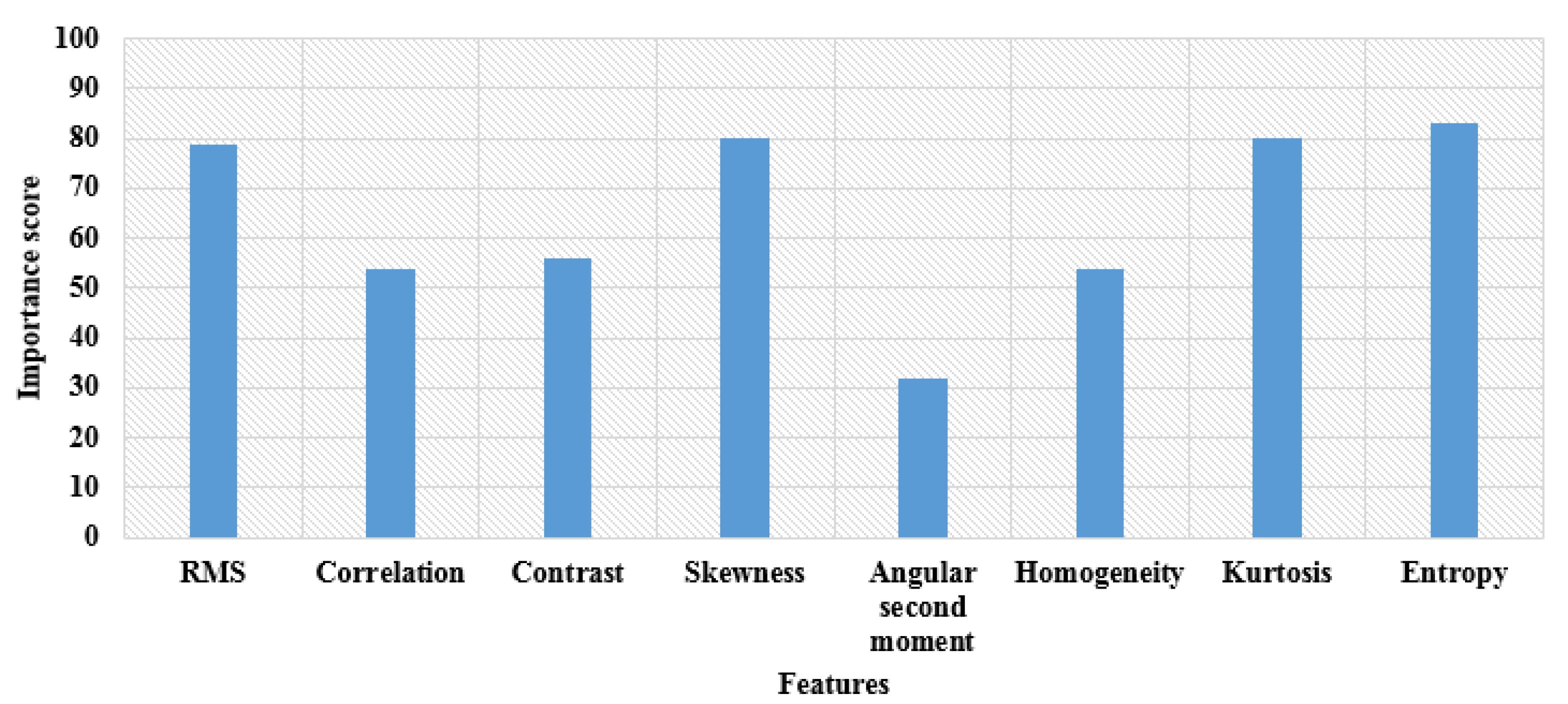
4.5. Analysis of Features on Statistical Errors

The analysis of the adopted EC scheme overrepresented the method without statistical features, the presented method without a novel hydro index, and the presented method without features as shown in

Table 3. Error statistics achieved by EC, which is trained by different features, in categorizing underground water levels and their conditions from 10-fold experimental validation.

	EC without Statistical Feature	EC without Novel Hydro Index	EC without Feature Extraction	Proposed EC
MCC	0.009	0.013	0.003	0.928
NPV	0.073	0.100	0.146	0.851
Specificity	0.046	0.044	0.051	0.929
FNR	0.053	0.054	0.053	0.021
F-measure	0.930	0.911	0.894	0.957
Accuracy	0.870	0.838	0.810	0.928
Sensitivity	0.946	0.945	0.946	0.925
FPR	0.953	0.955	0.948	0.008
Precision	0.915	0.880	0.847	0.920

. In Table 3, the NPV of EC is higher than the presented method without statistical features, the presented method without novel hydro index, and the presented method without features. Next to the EC scheme, the presented method without features has achieved superior NPV outcomes over the adopted method without statistical features and the presented method without a novel hydro index. Likewise, in Table 3, the FPR of EC is lesser (0.008) than the presented method without statistical features, the presented method without a novel hydro index, and the presented method without features. Next to the EC scheme, the presented method without features has achieved fewer FPR outcomes over the adopted method without statistical features and the presented method without a novel hydro index. Similarly, the F-measure of EC is high (0.957) over the presented method without statistical features, the presented method without a novel hydro index, and the presented method without features. Next to the EC scheme, the presented method without statistical features has achieved superior F-measure (0.930) outcomes over the adopted method without features and the presented method without a novel hydro index.

4.6. Discussion

One of the most vital natural elements is groundwater. In order to comprehend groundwater resources and maintain sustainable development of water resources and the environment, regional groundwater depth is a crucial parameter. Here, the Improved Hydro Index Value with Ensemble Classifier was used to evaluate the prediction of underground water levels in remote sensing images. A Wiener filter was developed for removing additive noise and blurring from obtained remote sensing images. The Wiener filter is best because it minimizes the total mean square error during the inverse filtering and noise smoothing processes. Statistical features and integrated VI, NDVI, NDSI, IRI, and RVI features were used for feature extraction. The effectiveness of predicting underground water levels using remote sensing images is improved by the discriminative extracted features, which reduce the sematic space between the feature subsets. Improved NN, SVM, and DCNN are included in the Proposed Ensemble Classifier (EC) model for accurate underground water level forecast. According to the findings, the suggested EC model’s False Positive Rate (FPR) is 0.0083, which is lower than that of current approaches. The proposed EC model, however, outperforms conventional models, including the Long Short-Term Memory (LSTM) network, Naive Bayes (NB), Random Forest (RF), Recurrent Neural Network (RNN), and Bidirectional Gated Recurrent Unit (Bi-GRU) with a high accuracy of 0.90.

5. Conclusions

This research suggested a new framework for predicting the underground level of water using remote sensing images. Firstly, a Wiener filter is used for preprocessing, and further, features including VI (NDVI, NDSI, IRI, and RVI) and statistical features (entropy, RMS, Skewness, and Kurtosis) are extracted from preprocessed images. Here, the VI and statistical features are combined as a novel hydro index. Finally, the extracted 3290 HI features are given to the EC model (NN, SVM, and improved DCNN) for underground water level prediction. According to the resulting findings, the proposed EC model’s False Positive Rate (FPR) is 0.0083, which is lower than that of conventional approaches. The proposed EC model, in contrast, has a high accuracy of 0.90, which is better than the conventional models. Further, the MCC of the EC model has gained a high value of 0.99 at the 90th LP, the NPV of the EC model is high at the 70th LP, and the next high NPV value of the EC model is obtained at the 90th LP with a value of 0.90. However, utilizing DL models raises many issues: DL models are frequently interpreted as black boxes that imply that it is very challenging to unravel and recognize the automatic feature selection process, which finally occurs, and the forecasts that emerge from any given DL-oriented schemes. They are also very expensive to train and utilize, regarding time and resources. In the future, this research will be further extended by analyzing various simulation settings with novel hybrid methods for feature selection.

References

1. Fathi, A.; Lee, T.; Mohebzadeh, H. Allocating Underground Dam Sites Using Remote Sensing and GIS Case Study on the Southwestern Plain of Tehran Province, Iran. J. Indian Soc. Remote Sens. 2019, 47, 989–1002. [Google Scholar] [CrossRef]
2. Yan, S.; Shi, K.; Li, Y.; Liu, J.; Zhao, H. Integration of Satellite Remote Sensing Data in Underground Coal Fire Detection: A Case Study of the Fukang Region, Xinjiang, China. Front. Earth Sci. 2020, 14, 1–12. [Google Scholar] [CrossRef]
3. Wang, X.; Guo, Z.; Wu, L.; Zhu, C.; He, H. Extraction of Palaeochannel Information from Remote Sensing Imagery in the East of Chaohu Lake, China. Front. Earth Sci. 2012, 6, 75–82. [Google Scholar] [CrossRef]
4. Fossi, D.H.; Djomo, H.D.; Takodjou Wambo, J.D.; Kouayep Tchoundi, L.C.; Deassou Sezine, E.; Takam Tchoupe, G.B.; Tchatchueng, R. Extraction and Analysis of Structural Lineaments from Mokolo Area, North Cameroon, Using DEM and Remote Sensing Images, and Their Influence on Drainage Morphometric. Arab. J. Geosci. 2021, 14, 2062. [Google Scholar] [CrossRef]
5. Guo, F.; Gao, Z. RETRACTED ARTICLE: Sponge City Plant Planning and Urban Construction Based on High-Resolution Remote Sensing Images. Arab. J. Geosci. 2021, 14, 1131. [Google Scholar] [CrossRef]
6. İrdemez, Ş.; Eymirli, E.B. Determination of Spatiotemporal Changes in Erzurum Plain Wetland System Using Remote Sensing Techniques. Environ. Monit. Assess. 2021, 193, 265. [Google Scholar] [CrossRef]
7. Siming, C.; Aidi, H.; Wenke, G. Remote Sensing Monitoring Method for Groundwater Level on Aeolian Desertification Area. J. Water Chem. Technol. 2020, 42, 522–529. [Google Scholar] [CrossRef]
8. Zacharias, I.; Dimitriou, E.; Koussouris, T. Quantifying Land-Use Alterations and Associated Hydrologic Impacts at a Wetland Area by Using Remote Sensing and Modeling Techniques. Environ. Model. Assess. 2004, 9, 23–32. [Google Scholar] [CrossRef]
9. Liu, H.; Jiang, Y.; Misa, R.; Gao, J.; Xia, M.; Preusse, A.; Sroka, A.; Jiang, Y. Ecological Environment Changes of Mining Areas around Nansi Lake with Remote Sensing Monitoring. Environ. Sci. Pollut. Res. 2021, 28, 44152–44164. [Google Scholar] [CrossRef]
10. Jha, M.K.; Chowdhury, A.; Chowdary, V.M.; Peiffer, S. Groundwater Management and Development by Integrated Remote Sensing and Geographic Information Systems: Prospects and Constraints. Water Resour. Manag. 2007, 21, 427–467. [Google Scholar] [CrossRef]
11. Joshi, P.K.; Kumar, M.; Midha, N.; Yanand, V.; Wal, A.P. Assessing Areas Deforested by Coal Mining Activities through Satellite Remote Sensing Images and Gis in Parts of Korba, Chattisgarh. J. Ind. Soc. Remote Sens. 2006, 34, 415–421. [Google Scholar] [CrossRef]
12. Sivasankar, T.; Borah, S.B.; Das, R.; Raju, P.L.N. An Investigation on Sudden Change in Water Quality of Brahmaputra River Using Remote Sensing and GIS. Natl. Acad. Sci. Lett. 2020, 43, 619–623. [Google Scholar] [CrossRef]
13. Lee, S.; Hyun, Y.; Lee, S.; Lee, M.J. Groundwater potential mapping using remote sensing and GIS-based machine learning techniques. Remote Sens. 2020, 12, 1200. [Google Scholar] [CrossRef] [Green Version]
14. Collignon, B. A New Tool for the Remote Sensing of Groundwater Tables: Satellite Images of Pastoral Wells. Open Geospat. Data Softw. Stand. 2020, 5, 4. [Google Scholar] [CrossRef]
15. Chowdary, V.M.; Ramakrishnan, D.; Srivastava, Y.K.; Chandran, V.; Jeyaram, A. Integrated Water Resource Development Plan for Sustainable Management of Mayurakshi Watershed, India Using Remote Sensing and GIS. Water Resour. Manag. 2009, 23, 1581–1602. [Google Scholar] [CrossRef]
16. Molla, M.H.; Chowdhury, M.A.T.; Islam, A.M.Z. Spatiotemporal Change of Urban Water Bodies in Bangladesh: A Case Study of Chittagong Metropolitan City Using Remote Sensing (RS) and GIS Analytic Techniques. J. Ind. Soc. Remote Sens. 2021, 49, 773–792. [Google Scholar] [CrossRef]
17. Cheng, C.; Zhang, F.; Shi, J.; Kung, H.-T. What Is the Relationship between Land Use and Surface Water Quality? A Review and Prospects from Remote Sensing Perspective. Environ. Sci. Pollut. Res. 2022, 29, 56887–56907. [Google Scholar] [CrossRef]
18. El Garouani, A.; Aharik, K.; El Garouani, S. Water Balance Assessment Using Remote Sensing, Wet-Spass Model, CN-SCS, and GIS for Water Resources Management in Saïss Plain (Morocco). Arab. J. Geosci. 2020, 13, 738. [Google Scholar] [CrossRef]
19. Jiang, H.; Liu, C.; Sun, X.; Lu, J.; Zou, C.; Hou, Y.; Lu, X. Remote Sensing Reversion of Water Depths and Water Management for the Stopover Site of Siberian Cranes at Momoge, China. Wetlands 2015, 35, 369–379. [Google Scholar] [CrossRef]
20. Majumdar, S.; Smith, R.; Butler, J.J.; Lakshmi, V. Groundwater Withdrawal Prediction Using Integrated Multitemporal Remote Sensing Data Sets and Machine Learning. Water Resour. Res. 2020, 56, e2020WR028059. [Google Scholar] [CrossRef]
21. Sureshkumar, V.; Somarajadikshitar, R.; Beeram, B.S. A Novel Representation and Prediction Initiative for Underground Water by Using Deep Learning Technique of Remote Sensing Images. Comput. J. 2022, bxac101. [Google Scholar] [CrossRef]
22. Wang, Z.; Tian, S. Ground Object Information Extraction from Hyperspectral Remote Sensing Images Using Deep Learning Algorithm. Microprocess. Microsyst. 2021, 87, 104394. [Google Scholar] [CrossRef]
23. Suganthi, S.; Elango, L.; Subramanian, S.K. Groundwater potential zonation by Remote Sensing and GIS techniques and its relation to the Groundwater level in the Coastal part of the Arani and Koratalai River Basin, Southern India. Earth Sci. Res. J. 2013, 17, 87–95. [Google Scholar]
24. Tao, H.; Hameed, M.M.; Marhoon, H.A.; Zounemat-Kermani, M.; Heddam, S.; Kim, S.; Sulaiman, S.O.; Tan, M.L.; Sa’adi, Z.; Mehr, A.D.; et al. Groundwater Level Prediction Using Machine Learning Models: A Comprehensive Review. Neurocomputing 2022, 489, 271–308. [Google Scholar] [CrossRef]
25. Shnewer, F.M.; Hasan, A.A.; AL-Zuhairy, M.S. Groundwater Site Prediction Using Remote Sensing, GIS and Statistical Approaches: A Case Study in the Western Desert, Iraq. IJET 2018, 7, 166–173. [Google Scholar] [CrossRef]
26. Zipper, S.C.; Gleeson, T.; Kerr, B.; Howard, J.K.; Rohde, M.M.; Carah, J.; Zimmerman, J. Rapid and accurate estimates of streamflow depletion caused by groundwater pumping using analytical depletion functions. Water Resources Research 2019, 55, 5807–5829. [Google Scholar] [CrossRef]
27. El-Hadidy, S.M.; Morsy, S.M. Expected Spatio-Temporal Variation of Groundwater Deficit by Integrating Groundwater Modeling, Remote Sensing, and GIS Techniques. Egypt. J. Remote Sens. Space Sci. 2022, 25, 97–111. [Google Scholar] [CrossRef]
28. Hussein, E.A.; Thron, C.; Ghaziasgar, M.; Bagula, A.; Vaccari, M. Groundwater Prediction Using Machine-Learning Tools. Algorithms 2020, 13, 300. [Google Scholar] [CrossRef]
29. Zhang, H.; Ma, J.; Chen, C.; Tian, X. NDVI-Net: A fusion network for generating high-resolution normalized difference vegetation index in remote sensing. ISPRS J. Photogramm. Remote Sens. 2020, 168, 182–196. [Google Scholar] [CrossRef]
30. Gascoin, S.; Dumont, Z.B.; Deschamps-Berger, C.; Marti, F.; Salgues, G.; López-Moreno, J.I.; Revuelto, J.; Michon, T.; Schattan, P.; Hagolle, O. Estimating fractional snow cover in open terrain from sentinel-2 using the normalized difference snow index. Remote Sens. 2020, 12, 2904. [Google Scholar] [CrossRef]
31. Gonenc, A.; Ozerdem, M.S.; Acar, E. Comparison of NDVI and RVI Vegetation Indices Using Satellite Images. In Proceedings of the 2019 8th International Conference on Agro-Geoinformatics (Agro-Geoinformatics), Istanbul, Turkey, 16–19 July 2019; pp. 1–4. [Google Scholar] [CrossRef]
32. Kim, Y.; van Zyl, J.J. A Time-Series Approach to Estimate Soil Moisture Using Polarimetric Radar Data. IEEE Trans. Geosci. Remote Sens. 2009, 47, 2519–2527. [Google Scholar] [CrossRef]
33. Koppe, W.; Gnyp, M.L.; Hütt, C.; Yao, Y.; Miao, Y.; Chen, X.; Bareth, G. Rice Monitoring with Multi-Temporal and Dual-Polarimetric TerraSAR-X Data. Int. J. Appl. Earth Obs. Geoinf. 2013, 21, 568–576. [Google Scholar] [CrossRef]
34. Wen, Q.; Liu, H.; Zhang, Z. A method of generating multivariate non-normal random numbers with desired multivariate skewness and kurtosis. Behav. Res. Methods 2020, 52, 939–946. [Google Scholar]
35. Martin, C.; Aleem, S.H.A.; Zobaa, A.F. On the root mean square error (RMSE) calculation for parameter estimation of photovoltaic models: A novel exact analytical solution based on Lambert W function. Energy Convers. Manag. 2020, 210, 112716. [Google Scholar]
36. Gawali, S. Shape of Data: Skewness and Kurtosis. 2021. Available online: https://www.analyticsvidhya.com/blog/2021/05/shape-of-data-skewness-and-kurtosis/ (accessed on 5 September 2022).
37. Yan, H.; Deng, H. An improved belief entropy in evidence theory. IEEE Access 2020, 8, 57505–57516. [Google Scholar] [CrossRef]
38. Mohan, Y.; Chee, S.S.; Xin, D.K.P.; Foong, L.P. Artificial Neural Network for Classification of Depressive and Normal in EEG. In Proceedings of the 2016 IEEE EMBS Conference on Biomedical Engineering and Sciences (IECBES), Kuala Lumpur, Malaysia, 4–8 December 2016; pp. 286–290. [Google Scholar] [CrossRef]
39. Avci, E. A New Intelligent Diagnosis System for the Heart Valve Diseases by Using Genetic-SVM Classifier. Expert Syst. Appl. 2009, 36, 10618–10626. [Google Scholar] [CrossRef]
40. Gu, J.; Wang, Z.; Kuen, J.; Ma, L.; Shahroudy, A.; Shuai, B.; Liu, T.; Wang, X.; Wang, G.; Cai, J.; et al. Recent Advances in Convolutional Neural Networks. Pattern Recognit. 2018, 77, 354–377. [Google Scholar] [CrossRef] [Green Version]
41. Rohde, M.M.; Biswas, T.; Housman, I.W.; Campbell, L.S.; Klausmeyer, K.R.; Howard, J.K. A Machine Learning Approach to Predict Groundwater Levels in California Reveals Ecosystems at Risk. Front. Earth Sci. 2021, 9, 784499. [Google Scholar] [CrossRef]
Figure 1. Diagrammatic depiction of the developed underground water level prediction model.
Remotesensing 15 02015 g001
Figure 2. Analysis of statistical feature importance.
Remotesensing 15 02015 g002
Figure 3. Images of regions where the underground water level is in critical condition. (a,b) Images of two different regions and (c,d) preprocessed image using Wiener filtering.
Remotesensing 15 02015 g003aRemotesensing 15 02015 g003b
Figure 4. Images of regions where the underground water level is highly exploited i.e., overconsumed. (a) Sample image 1 and (b) sample image 2. (c) Preprocessed image 1 by using Wiener filtering. (d) Preprocessed image 2 by using Wiener filtering.
Remotesensing 15 02015 g004
Figure 5. Images of regions with Safe water level. (a) Original image 1 and (b) original image 2. (c) Preprocessed image 1 by using Wiener filtering. (d) Preprocessed image 2 by using Wiener filtering.
Remotesensing 15 02015 g005
Figure 6. Images of regions with salinity (saline water). (a) Original image 1 and (b) original image 2. (c) Preprocessed image 1 by using Wiener filtering. (d) Preprocessed image 2 by using Wiener filtering.
Remotesensing 15 02015 g006
Figure 7. Images of regions with Semi-critical. (a) Original image 1 and (b) original image 2. (c) Preprocessed image 1 by using Wiener filtering. (d) Preprocessed image 2 by using Wiener filtering.
Remotesensing 15 02015 g007