Article

Rockfall Magnitude-Frequency Relationship Based on Multi-Source Data from Monitoring and Inventory

1
Institut Cartogràfic i Geològic de Catalunya (ICGC), 08038 Barcelona, Spain
2
Department of Civil and Environmental Engineering, Universitat Politècnica de Catalunya-BarcelonaTech, 08034 Barcelona, Spain
3
Univ. Grenoble Alpes, Univ. Savoie Mont Blanc, CNRS, IRD, Univ. Gustave Eiffel, ISTerre, 38000 Grenoble, France
4
Departament de Dinàmica de la Terra i de l’Oceà, GRC RISKNAT, UB-Geomodels, Facultat de Ciències de la Terra, Universitat de Barcelona (UB), 08028 Barcelona, Spain
*
Author to whom correspondence should be addressed.
Remote Sens. 2023, 15(8), 1981; https://doi.org/10.3390/rs15081981
Submission received: 5 February 2023 / Revised: 27 March 2023 / Accepted: 4 April 2023 / Published: 9 April 2023
(This article belongs to the Special Issue Remote Sensing for Rock Slope and Rockfall Analysis)

Abstract

:
Quantitative hazard analysis of rockfalls is a fundamental tool for sustainable risk management, even more so in places where the preservation of natural heritage and people’s safety must find the right balance. The first step consists in determining the magnitude-frequency relationship, which corresponds to the apparently simple question: how big and how often will a rockfall be detached from anywhere in the cliff? However, there is usually only scarce data on past activity from which to derive a quantitative answer. Methods are proposed to optimize the exploitation of multi-source inventories, introducing sampling extent as a main attribute for the analysis. This work explores the maximum possible synergy between data sources as different as traditional inventories of observed events and current remote sensing techniques. Both information sources may converge, providing complementary results in the magnitude-frequency relationship, taking advantage of each strength that overcomes the correspondent weakness. Results allow characterizing rockfall detachment hazardous conditions and reveal many of the underlying conditioning factors, which are analyzed in this paper. High variability of the hazard over time and space has been found, with strong dependencies on influential external factors. Therefore, it will be necessary to give the appropriate reading to the magnitude-frequency scenarios, depending on the application of risk management tools (e.g., hazard zoning, quantitative risk analysis, or actions that bring us closer to its forecast). In this sense, some criteria and proxies for hazard assessment are proposed in the paper.

1. Introduction

This paper is focused on the characterization of rockfall hazard scenarios using the magnitude-frequency relationship as the first step of any hazard and risk quantitative analysis. This task corresponds to relating the magnitude of potential rockfall events to their occurrence probability or frequency, which is based on the rockfall activity in the past. This basic data can be obtained both with traditional methods of inventory and nowadays thanks to monitoring with remote sensing techniques. This is the context presented in the following introductory section.

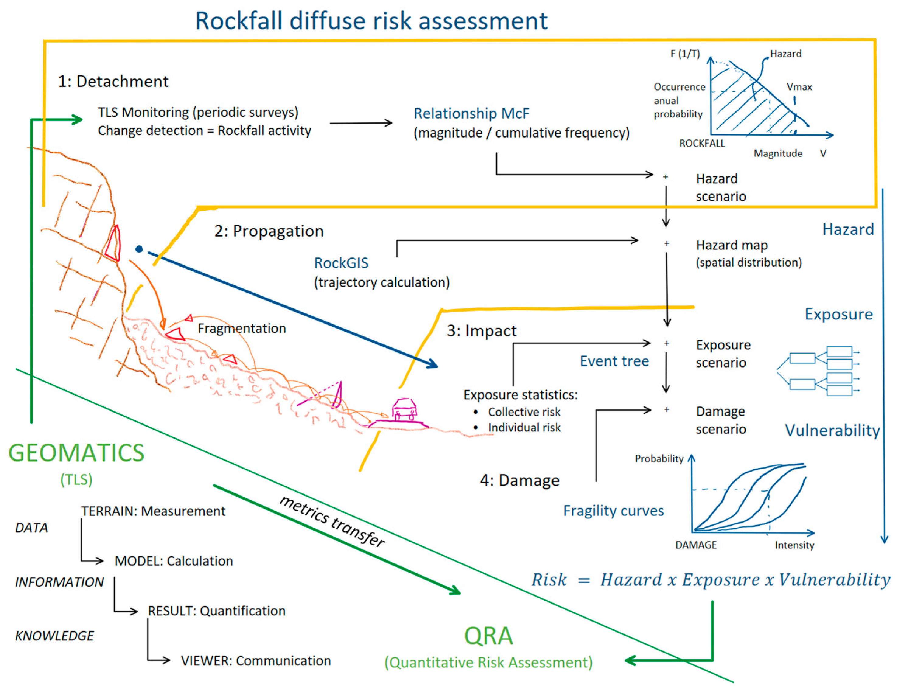
1.1. Magnitude-Frequency Relationship for Quantitative Assessment

Risk conceptualization and assessment are complex tasks because of the inherent uncertainties, and rockfall, as a stochastic natural process, is not an exception. Risk in geohazards is a concept that is often approached by society from an emotional point of view, either minimizing or maximizing it. If risk management and its communication to stakeholders are conducted in these terms, it can arbitrarily lead to imprudence or blocking, both equally unjustified. Instead, quantitative risk analysis (QRA) should provide an objective tool for risk management [1,2,3,4,5,6]. The complete procedure for rockfall QRA can be summarized in four stages (Figure 1):
  • Detachment: starting zone characterization to stabilize instability scenarios on the rock face dealing with rockfall initiation. The questions are: which events of a certain magnitude should be expected, and what is their probability of occurrence?
  • Propagation: trajectory analysis to map the resulting hazard distribution. In this step, it is critical to consider fragmentation, which modulates both the probability and intensity of impact. Rockfall simulation is required.
  • Impact: exposure considerations are to be cross checked with the hazard under several conditions, either from the perspective of individual or collective risk. The consideration of all possible damage scenarios can be addressed using event trees.
  • Damage: vulnerability analysis to estimate the intensity of damage for each element type in statistical terms. Fragility curves help to raise the uncertainty in this last step.
Based on previous research [7], two distinct analyses of rockfall hazards can be distinguished: diffuse and focused hazard analysis. While the approach to focused hazards tries to answer the question, “Is this single block unstable?” and “How unstable is it?”; for diffuse hazards, the question is another one: “How big and how often will a rockfall be detached from anywhere in the cliff?”. Geomatic remote sensing techniques, such as LiDAR or photogrammetry, can be used by both approaches to try to answer these questions [8,9,10,11]. When applied as monitoring techniques for change detection, rock surface deformation can be read as instability indications for focused analysis, and rockfall detection provides activity sampling for the frequency analysis of diffuse hazards. A broader state of the art on rockfall hazard assessment can be found in [10].
This paper aims at diffuse hazard analysis and is part of the Georisk project entitled “Advances in rockfall quantitative risk analysis (QRA) incorporating developments in geomatics” (www.georisk.upc.edu, accessed on 5 April 2023). The diagram in Figure 1 shows the scope of the project and the main objective of taking advantage of new geomatic developments for transferring metrics to risk analysis. At this point, remote sensing allows us the detection of rockfall activity (location and dating), as well as the measurement of detached volume or its magnitude [12]. Consequently, it provides both data necessary for magnitude-frequency analysis. Along with rockfall propagation, fragmentation may frequently occur [13]. Then, we can either measure the volume in the compact rock compartment before detachment or by summing the volume of all the resulting blocks at each run-out position. In the case of measuring the deposit volume as a whole, it will be possible to obtain the apparent expanded volume, including the porosity between fragments, which is necessary to make the appropriate correction. It must be distinguished between the size distribution of blocks resulting from fragmentation of one or superposed events [14], and the size distribution over time of total detached volume, the latter being the focus of this article.
Therefore, magnitude does not report the movement but only the dimensions of the initial trigger. Likewise, the magnitude-frequency relationships are the genuine expression of the probability of occurrence of rockfall release according to their size. This results from the properties of the rock mass and escarpment and the geodynamic and climatic context that causes the triggering actions. In this formulation, subsequent propagation is not considered, which will depend on the morphology and conditions of the slope located below the escarpment. Thus, the magnitude-frequency relationship does not fully express the idea of hazard but only its initial conditions, which should be more precisely called detachment hazard scenarios. In the rest of the text, we will use the notation McF to denote the relationship between magnitude and its cumulative frequency. McF has been analyzed for all landslide types [3,15,16,17,18,19,20]. According to the recent review of this issue specifically for rockfalls by [21], our approach is equivalent to the so-called McF methods.

1.2. Rockfall Activity Detection and Registration

In the diffuse risk analysis, rockfall is considered a recurrent phenomenon distributed over time and space. Thus, it is assumed that its frequency can be derived from past activity as a representative characterization also for the future, while the underlying conditions remain invariant. Therefore, the frequency analysis is based on the register of rockfall activity. Observing an event either directly or retrieved by survey, a documentary record, a land photographic register, or remote sensing and monitoring are commonly used methods for acquiring this type of data. Some additional considerations are detailed in Supplementary Material SM1. Except in the case of direct observation, it is necessary to do a certain process of extracting information from the available data, and this process will determine the properties of the inventory obtained. Whatever the data source, a perfect record of landslide activity is never obtained. In landslides, there is a current trend to combine the detection capabilities of remote sensing with processing using machine learning techniques [22,23].
In reporting rockfall activity, each record corresponds to an event, understood as a single rockfall, either a monolithic block or a disintegrated rock mass. However, they are physically connected in the same failure mechanism and with a simultaneous or continuous fall. We consider the following criteria into account in different cases: Despite having the same trigger (as is sometimes the case during an earthquake), simultaneous rockfalls from various points are distinct events. Even though it may make sense to consider them as progressive failure, rockfalls that occur near together but at different times due to various trigger pulses are considered separate events. For subsequent exploitations of the inventory, it is desirable to have additional fields of the conditions under which they occur (e.g., environmental conditions, identified triggers, linkage in progressive ruptures). However, for the McF analysis that we aim to conduct, three essential data points must be obtained from each event:
  • Where? The localization of the detachment point. In rockfall from vertical cliffs, xyz coordinates are needed, as xy coordinates on digital terrain models incur a great deal of indeterminacy in the elevation. To determine the spatial representativeness, at least each rockfall is needed to be linked to a cliff sector that will determine the spatial resolutions of the analysis.
  • When? The accuracy of the dating of events can be highly variable depending on the data source, from imprecise references in years to detailed dates and times. For the annual frequency calculation, we simply need the dating by years, but this is not the case in triggering factor analyses.
  • How big? This is the feature to be analyzed for hazard scenario assessment. It is expressed in the total volume of rock detached from the cliff as a single rockfall event.
Since the accuracy of these three components can be very variable, it is convenient to enrich inventories with auxiliary fields describing the accuracy of each variable independently, either numerically or qualitatively in typical cases, to reflect the interpretation process employed until data are registered. It is also important to consider the completeness of the inventory as a whole and even its heterogeneity according to the data sources used.

1.3. Remote Sensing in Rockfall Problems

A comprehensive review of remote sensing techniques for rockfall research is beyond the scope of this article, however, it is accessible in [8,10,24,25,26]. Other remote sensing systems are reported in [24,27,28,29,30,31]. Among them, two technologies are becoming predominant in rockfall analysis due to their versatility: LiDAR and photogrammetry, both of which provide 3D point clouds of the object’s surface, including the ground [24,27,32]. The combination of these two techniques on different platforms (terrestrial and airborne, lately from drones), providing complementary points of view (frontal, oblique, and zenithal), constitutes a complete remote sensing system for rockfall characterization [8,25,28,33]. The recent irruption of UAVs (unmanned aerial vehicles) in geosciences [34,35] has greatly facilitated access to oblique views, which are particularly useful in the study of rockfalls [36,37]. For the test sites in this paper (Section 3), we are using LiDAR monitoring data, in particular from a terrestrial laser scanner (hereafter TLS), which allows a frontal view of vertical cliffs from opposite slopes or viewpoints at their bottom.
The products that can be derived from rockfall 3D models/clouds cover the successive analysis steps: morphology and susceptibility of the slope; terrain surface for trajectory calculation and roughness consideration; rock mass structure and rupture mechanisms; volume measurement of potentially unstable masses and scars on the wall; volume measurement of deposits and fallen blocks; monitoring for the detection of rockfall activity; and monitoring for the detection of surface displacements as precursor signs of instability [38,39,40,41,42,43].

1.4. Objectives and Content

In accordance with the scope presented in this introduction, the main objective of this study is specified as optimizing the exploitation of rockfall inventories for hazard assessment. We intend to cross check the results of traditional inventories and monitoring to leverage each other and determine their complementarity. Specific objectives cover other related issues:
  • Hazard variability over time is due to triggering conditions and other evolving factors.
  • Hazard variability at different scales from outcrop to massif.
  • Influence of other factors on rockfall detachment conditions and related hazards.
All these investigations aim to better understand factors that influence the preparation and triggering of rockfalls, with the horizon set in their forecast to enrich risk management strategies. After this introductory section, the content of the paper is structured as follows: In Section 2, the methodology that will be applied is summarized, and the sampling extent feature is introduced. In Section 3, the case sites used as examples for the developments are presented with their rockfall activity samples obtained by monitoring and inventory. These data are analyzed in Section 4 separately by each source type to take into consideration the limitations encountered, apply appropriate treatments, and make the most of the available data. The results in terms of magnitude-frequency relationships are presented, and in Section 5 the main findings are discussed in view of the various applications to hazard assessment oriented to rockfall risk management before concluding.

2. Methods

The main definitions and formulations for McF analysis follow in this section.

2.1. Methodological Basis

According to the glossary in use [3,12], the rockfall magnitude is the volume V of the total detached mass in a single event, and its frequency is expressed in inverse cumulative terms, F V = F ( V o l u m e V ) . This formulation corresponds to the fact that we are not interested in the probability of any case of a specific size, but of all cases large enough to cause a certain level of effects. Under uniform and constant conditions of the rock mass and wall, the frequency increases proportionally to the period and extension of the source area. Therefore, frequency is normalized to spatial-temporal cumulative frequency, F s t V , being expressed in normalized units, h m 2 · y e a r 1 , where the source area extension is computed in h m 2 and the time span in y e a r s [7]. This way, F s t V describes the cliff activity in terms of the pursued McF. Multiple rockfall hazard studies in the last 25 years [19,44,45,46,47,48,49,50,51,52,53] have established that the distribution of detached volumes can be adjusted by a power law such as F s t V = A s t · V B , in which two parameters describe the rockfall activity of the rock cliff:
  • A s t 
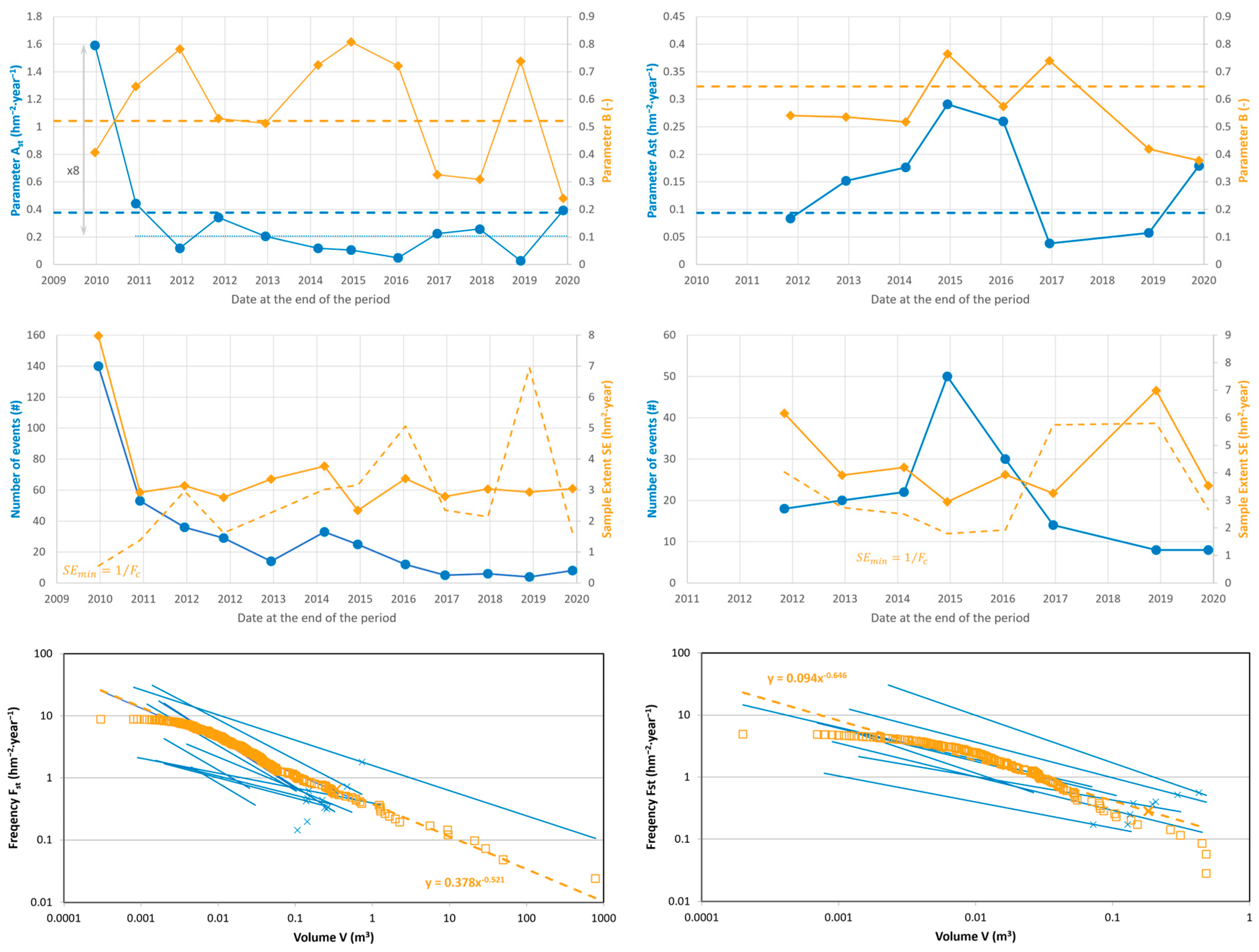
is the normalized or unitary activity, as A s t = F s t 1 , being the number of rockfalls of V 1 m3 detached from 1 hm2 of cliff surface in 1 year. It is a significant normalizing case since in most situations, this size is both frequent and destructive enough to be considered a reference.
  • B is the uniformity coefficient in the volume distribution. The greater the B , the greater the reduction in probability when going from small to large rockfalls. By definition of cumulative frequency, B > 0 , and the negative sign of the exponent is already introduced in the equation.
In Supplementary Material SM2, more details on McF power law are highlighted. There, we define the center of the hyperbola as the point where the curve F s t is orthogonal to the bisector line of the first quadrant ( F s t = 1 ), which is placed on the volume value V c = A s t · B 1 / B + 1 . By center definition, for volume values V V c , small linear variations in volume correspond to a larger change in frequency, and, inversely, for V V c large linear variations in volume have a small influence on the corresponding frequency. In other words, uncertainty in volume plays a more significant role on the left side than on the right, which leads to the necessity of measuring properly small volumes using TLS monitoring as an appropriate tool. The center does not necessarily correspond to the point of the hyperbola closest to the coordinate origin 0,0 ; instead, we call this point the origin of the hyperbola that is placed at, V 0 = A s t 2 · B 1 2 B + 1 , and this minimum distance is d 0 = V 0 1 + 1 / B .
As established by [7], the integration of the area below the hyperbola corresponds to the erosion rate, which is a proper descriptor of the detachment hazard of the outcrop. This calculation requires establishing upper and lower limits of plausible volumes linked to the characteristics of the massif and the slope [49]. Without considering these magnitude thresholds, the hazard cannot be fully concluded, but the center of McF describes the central part of the hazard and can be used to compare different case sites. For this purpose, two features of the hyperbola can be derived: from its origin ( d 0 , already introduced) and from its center ( p c , as the product of both coordinates of the center). It can be seen that p c = V c · F s t V c = A s t A s t · B 1 B 1 + B . In this paper, the center, V c ; F c , is used to describe McF by one point instead of a line to easier compare different case sites and to see how rock mass and environmental conditions influence the hazard potential. As seen in Section 5, without considering the truncated curve at the maximum expected magnitude, V m a x , that would provide the true meaning of hazards and erosion rates. Under this assumption, p c and d 0 are suggested as proxies for the intrinsic hazard of the slope before considering the geometry of the outcrop.

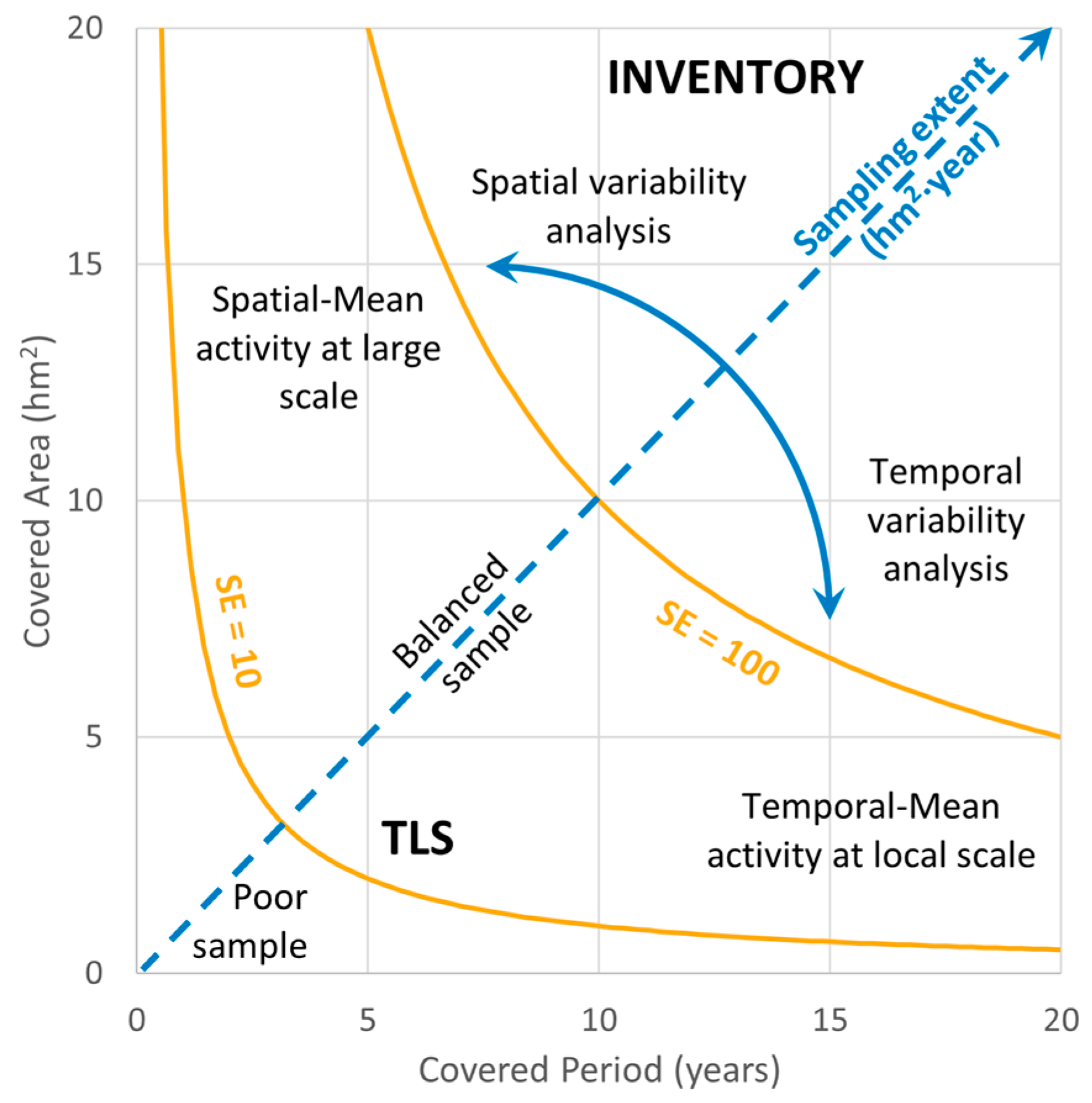
2.2. Sampling Extent

Rockfall inventories are registers of its activity covering a specific time span c t and source zone area c a , which are needed to be assessed for computing F s t . Furthermore, they define the sample contained in the inventory. In this manner, the sampling extent S E is defined as follows:
S E s a m p l i n g   e x t e n t = c o v e r e d   a r e a h m 2 × c o v e r e d   p e r i o d   y e a r
Very frequent rockfall activity is well characterized by samples of low S E , but not the infrequent activity or exceptional events in which we are particularly interested in hazard assessment. Then, a large S E is required, which can be provided by a time span or covered area (Figure 2). The bisector axis represents S E as the product of both axes (spatial and temporal). In this kind of graph, rockfall inventories can be represented to quickly see their attributes. Samples of equal S E are placed on a hyperbolic curve, and their distance from the bisector axis shows if they are time-over-space enriched samples or in reverse. On this graph, inventories obtained by the different data sources previously presented can be compared. Monitoring inventories, such as those from TLS, tend to be local and short samples, while observational inventories tend to build a sample with larger coverage in space and time, but then the problem is making sure it is complete. We propose merging rockfall inventories from different data sources to take advantage of the completeness of monitoring inventories and the representativeness of observational and historical inventories. This is because the longer the time span, the more confidence there is in calculating return periods. As declared in Section 1.4, we attempt to extract as much detail as possible about the spatial and temporal variability of hazards, such as [54]. Thus, we attempt combining multi-source data to compensate for the shortcomings of one source and another and to cover the widest magnitude range possible, such as [55]. The introduction of S E in the analysis allows us to achieve this since it characterizes the samples when combining them. S E happens to be an attribute of the recorded events, in which the extent of the rockfall has been detected and recorded.
Finally, it should be noted that the S E value, which allows obtaining a sufficient sample to characterize the activity, depends on the degree of the activity itself. In places or periods—both variables will be analyzed in this paper—of great activity, a small sampling area and period of time are sufficient to obtain a sufficient sample, whereas, in places or periods of minimal activity, it is necessary to expand the sampling to achieve a sufficient level of representativeness. Therefore, it is convenient to put S E in relation to the parameter, A s t , in such a way that we introduce the unitary sampling extent as S E u A = S E · A s t , which is dimensionless. Note that it is the expected number of rockfalls larger than 1 m3 to be registered by the sample. In Figure 3, samples of case sites analyzed in this paper and presented in the next Section 3 are shown this way. Every sample can be rapidly characterized by S E u A , because S E u A < 1 means that there is no sample larger enough to expect collected events larger than 1 m3 and to be confident with the A s t value. Alternatively, F c could be also used to normalize S E spite less intuitively. In that case, if S E u c = S E · F c 1 , the sampling extent covers appropriately the central part of the hyperbola, providing confidence in the obtained B value.
Another key feature of inventories obtained by rockfall monitoring is the sampling interval, as pointed out by [51,53], which should consider the scope of the monitoring. To perform trigger analysis, continuous monitoring is required. However, for McF analysis, discontinuous monitoring is preferred to maximize covered S E . The surveying period S P should be put in relation to the activity level ( A s t ) at the site. If surveys are planned with S P = V m i n B / A s t , it will be expected to mean one single event of V V m i n within a unitary source area of 1 hm2. In case sites such as those considered in this paper have A s t = 0.1 and B = 0.5 , a surveying period of 0.3 years would be appropriate to unequivocally identify rockfalls larger than V m i n = 10 3   m 3 .

3. Test Sites and Data

The test sites in this paper are Montserrat Massif and Castellfollit de la Roca Cliff, where ICGC is currently conducting monitoring with TLS for rockfall risk mitigation projects, which must meet the requirements of both safety and the preservation of the natural heritage. For this reason, research is being carried out in monitoring aimed at rockfall forecasts on which to base future sustainable risk management strategies. Monitoring was performed with two different TLS devices (see Table 1) offering similar performances: Optech from the beginning in 2007/08 and the Leica P50 from 2018.
The Montserrat Massif and Castellfollit de la Roca are excellent examples of both sorts of rockfall risks. The Montserrat Massif is an example of a location where boulders fall down a slope and impact with great force, while Castellfollit de la Roca is an example of a location where rockfalls cause the escarpment to retreat, which can lead to the collapse of constructions atop the cliff. In both cases, McF’s analysis helps us define hazard scenarios for subsequent risk management and communication. As claimed by [21], the main characteristics of the test sites can be found in Supplementary Material SM3, and more details on rockfall issues follow in the next subsections.

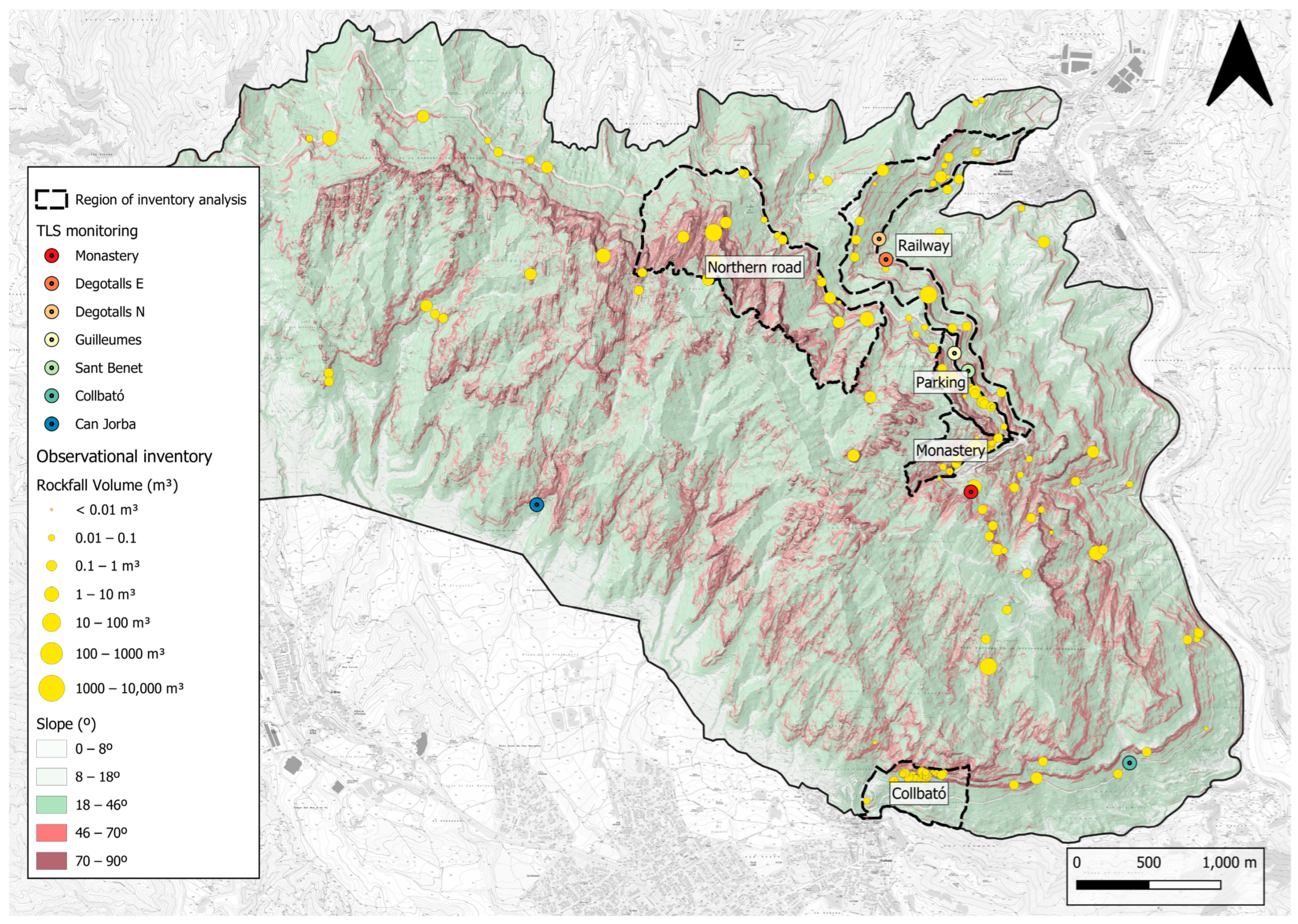
3.1. Conglomerate Massif in Montserrat

Montserrat is an isolated mountain placed 40 km inland from Barcelona, Catalonia, in the northeastern part of Spain. This massif is formed by thick layers of conglomerate interleaved by siltstone/sandstone from a Late Eocene fan delta along the southeastern margin of the Ebro Foreland Basin and adjacent to the Catalan Coastal Ranges [56]. At present, it emerges as inverted relief over the Llobregat River with an overall height difference of 1000 m (from 200 to 1200 m.a.s.l.). This configuration leads to the characteristic relief of staggered slopes, where vertical cliffs of conglomerate alternate with steep slopes of softer ground covered by densely vegetated colluvial deposits.
The mountain is a natural park due to its geological and biological assets and covers an extension of 35 km2. Moreover, at mid-height, there is a thousand-year-old monastery with a long and intense religious and cultural tradition. The double interest for tourists and hikers, together with the proximity to the metropolitan region of Barcelona, produces a great deal of frequentation in this small massif. This exceeds 3 million visitors, who concentrate especially in the vicinity of the monastery and sanctuary and in other places throughout the park. This exposure, combined with inherent geohazards, has demonstrated the risk for the building area and the terrestrial accesses, both roads and a rack railway. This risk was highlighted in the events of 2007–2008 in Degotalls affecting terrestrial accesses to monasteries and in 2010 affecting a building on the monastery grounds, which prompted first efforts to move from reactive to preventive actions [57].
Rock mass outcrops are represented by walls and needles, where rockfalls are generated. To assess the spatial variability of hazards all over the Montserrat Massif, slope units were established and called “slope domains.” Their delineation similarly follows the half-basin to [58], which is additionally crossed by the horizontal stratigraphic levels of main conglomerate units leading to 1070 domains. Since the relief is staggered, rockfall source areas are properly discretized through these domains. Rockfall source areas are identified following the approach of geomorphometric analysis of slopes proposed by [59]. In Montserrat, two morphological units are identified as rockfall source areas: inclined rock walls s l o p e 46 ° ; 70 ° and vertical walls s l o p e 70 ° ; 90 ° , with s l o p e being the raster derived from the 2.5D terrain elevation model. For the entire Montserrat Mountain and natural park, the sum of the rockfall source area is 1088 hm2. The dominant morphological unit is s l o p e 18 ° ; 46 ° , which corresponds to steep slopes where rockfalls propagate and form colluvial deposits.

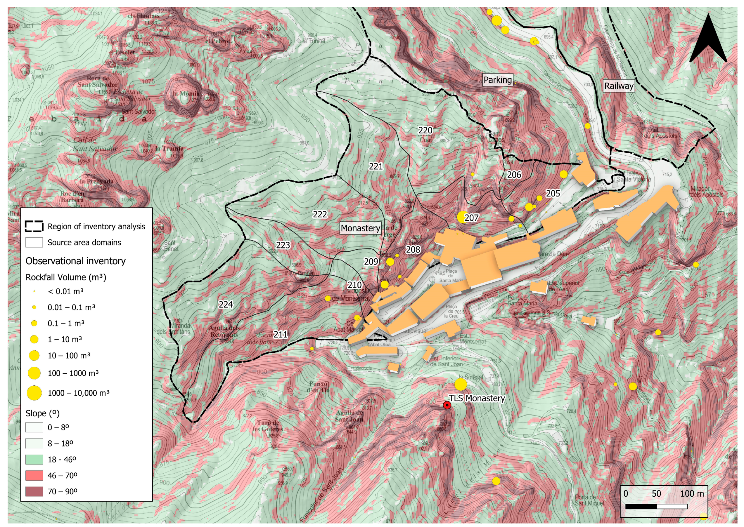
3.1.1. Observational Inventory

As part of the risk mitigation plan, an inventory was launched in 2014 to record the activity of geological risks in Montserrat, including rockfalls, shallow landslides, and torrential flows. It is a local scale inventory fed by different sources of information. On the one hand, a surveillance task is carried out consisting of periodic field inspections covering specific areas of interest and also being reactive to rainfall episodes. On the other hand, another way to obtain information is to search and extract from documents of heterogeneous nature. Recently, the inventory has been reviewed to improve homogeneity in the quality of the information. At this stage, three fields have been added to the DB that qualitatively describe the accuracy of the assessment of the three variables of the event vector (location, dating, and volume). The sample is formed by a total of 222 rockfalls that occurred between the years 1546 and 2020, with volumes ranging from 2 × 10⁻⁴ to 2.2 × 10³ m3, distributed throughout the massif with greater concentration in areas with higher human presence (Figure 4). The sample after filtering useless data (8%) is formed by a total of 205 rockfalls associated with only 97 slope domains. Accordingly, five zones have been selected for McF analysis, where the highest density of data is achieved because rockfalls directly affect infrastructures of major interest (Figure 4). They total 236 hm2 of rockfall source area or 22% of the total in Montserrat. Despite having recovered an event from the 16th century, it can be called “young inventory,” which has not been able to go back much in time since 92% of the records are from the 21st century. In terms of magnitude, 48% have a volume of less than 1 m3, 34% are between 1 and 10 m3, and the remaining 18% are greater than 10 m3. The inventory in Montserrat is estimated to have a total value of S E = 5156   h m 2 · y e a r .

3.1.2. TLS Monitoring

TLS monitoring started in May 2007, after a large rockfall in the Degotalls section of the monastery parking that affected both the road and the railway that has a parallel track 115 m down the slope. The progressive failure at this point of the wall led to another rockfall in December 2008, which is the largest event captured by TLS (before and after scanners were available) until the present. As part of the mitigation plan, other local sites have been progressively added to the monitoring system [26], until there are currently twelve stations, from which the seven longest series are included in this study (Figure 4). The most common period between surveys is about 6 months, although it was reduced to half for two years (2015–2016) looking for seasonal variations of rockfall activity, which was not clearly observed. The rock wall covered surface is mostly around 1 hm2, except for the panoramic view on the wall above the Monastery area from Fra Garí viewpoint, which is the triple. Due to the combined effect of coverage in space and time, S E varies by up to an order of magnitude depending on the station. Table 2 describes the main attributes of the sample obtained with TLS in Montserrat. In total, 592 rockfalls have been detected, which cover a wide range of six orders of magnitude.

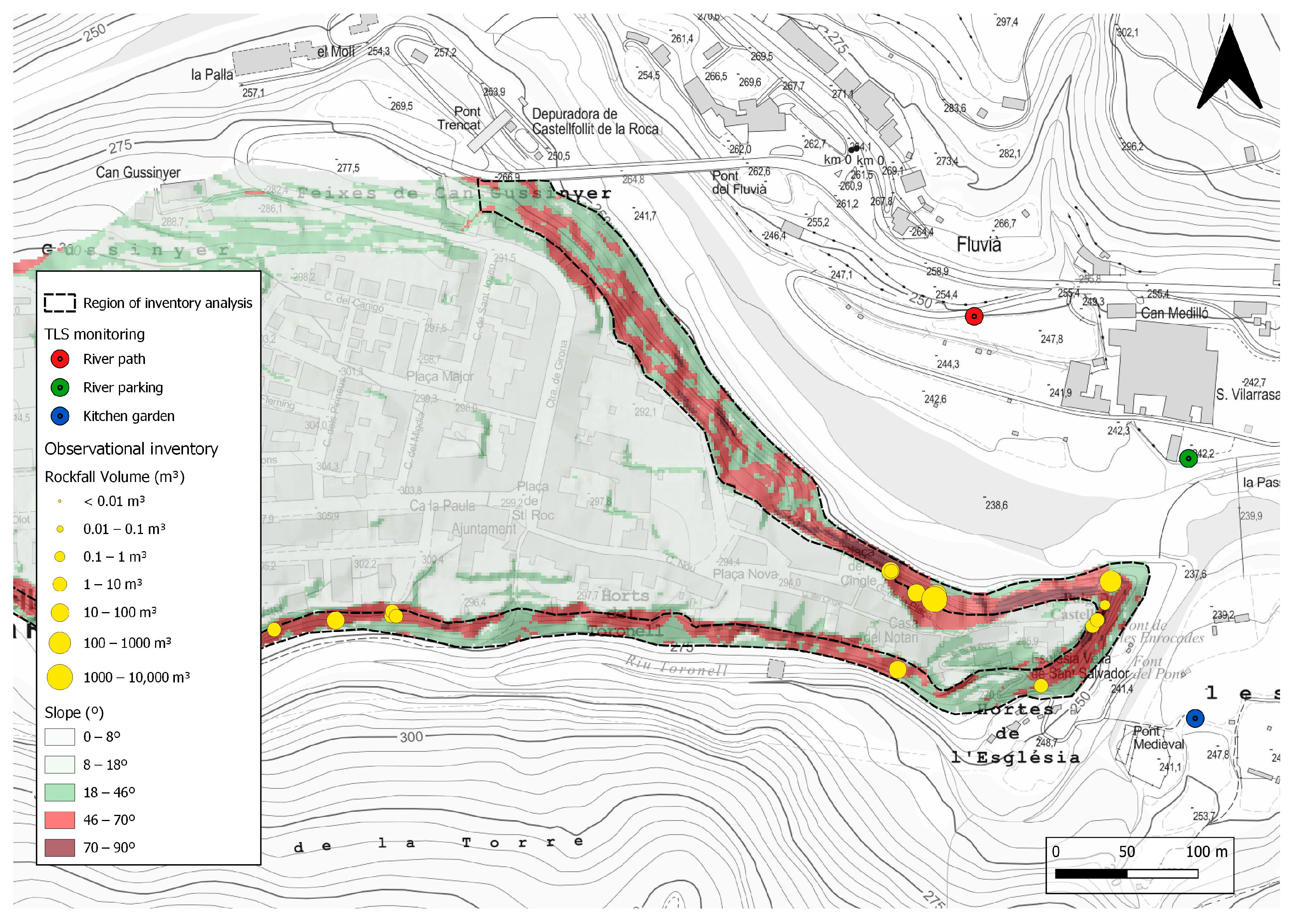
3.2. Basaltic Cliff in Castellfollit de la Roca

Castellfollit de la Roca is a village of 940 inhabitants located 40 km inland from Girona, Catalonia, in the northeastern part of Spain. This small municipality in extension (0.7 km2) is limited to the built-up center of medieval origin, defensively placed on a raised hill. This relief is caused by a Quaternary basaltic formation, which is the overlap of two lava flows from around 200,000 years ago that were separated by 20,000 years and a thin layer of paleosol, which makes a weak spot in the whole rock massif. The later erosive fluvial incisions on its banks (the main river Fluvià at the north flank and a tributary river, Toronell, at the south) have shaped the elongated cliffs that surround the entire hill [60]. This process has resulted in a basaltic cliff of up to 40 m in height and around 1200 m in perimetral length, which is currently one of the main geomorphological highlights of the natural park of the Garrotxa Volcanic Field and has a high value as a natural and cultural landscape.

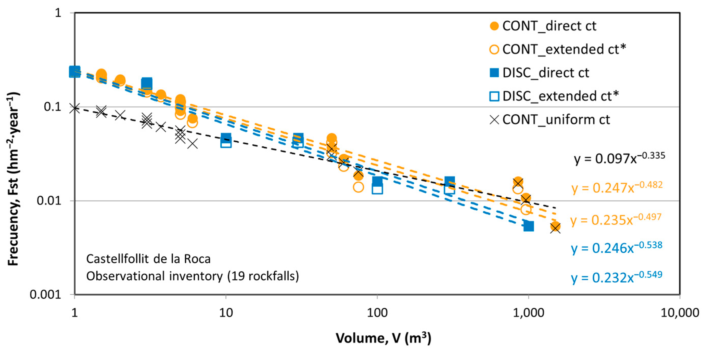
3.2.1. Observational Inventory

An observational inventory in Castellfollit has been built based on historical data compiled by recent documents on the local rockfall risk, whether academic studies or technical reports. There are some historical clues about the clifftop withdrawal over the centuries, but so far, no clear data on rockfall events have been found. A low-intensity surveillance task is carried out in parallel to TLS monitoring, which does not provide significant additional data. Until 2020, the inventory recorded 19 rockfall events, including large magnitude ones in 1976 and 2011. The list can be found in Supplementary Material SM3.

3.2.2. TLS Monitoring

In March 2006, TLS monitoring began in Castellfollit de la Roca. Based on the previous work [61], subsequent TLS monitoring has been able to detect both rockfall activity and precursory displacements. In this way, although the survey cadence is variable, a series of data from 2008 to 2020 has been obtained and is discussed here. The three operational TLS stations in Castellfollit (Figure 5) cover a significant extent of the northern side of the town, corresponding to the main cliff. On the other hand, there is no monitoring available of the cliff on the south side since it is a densely vegetated ravine that does not allow views suitable for remote sensing.
Table 3 describes the main attributes of the sample obtained with TLS in Castellfollit de la Roca, which totals S E = 33.14   h m 2 · year . In total, 298 rockfalls have been detected since 2008 with sizes between 2 × 10⁻⁴ m3 and 6 × 100 m3, which cover a limited range of four orders of magnitude because any large event in the inventory coincided with the scope covered by monitoring.

4. Data Analysis for McF Results

The data presented in the previous Section 3 are analyzed separately according to their source: both TLS monitoring (Section 4.1) and observational inventory (Section 4.2).

4.1. Monitoring Data Analysis

Characterizing the subsamples with their own sample extent S E i allows us to group the data into a single sample that will have the aggregate extent S E = i S E i , as long as the areas are not overlaid. Considering the sum of the wall surfaces covered by the different TLS locations, we obtain the equivalent sampling period of this integrative sample, which is a mean value weighted by each surface coverage, as seen in Table 2 and Table 3. Implicitly assuming that sectors are compatible, this fusion aims to be representative of a geographic entity at an upper scale and for a certain period. At the outset, quite similar rockfall activity can be observed in Castellfollit and Montserrat, with values between 6 and 9 rockfalls per year and per hm2 of the wall. However, it is necessary to see the distribution of volumes to translate these values in terms of hazards. The spatial–temporal cumulative frequency distribution, F s t , of the global set of TLS monitoring in Castellfollit de la Roca is shown in Figure 6. A very good fit is observed for a potential law in the wide central range of the sample, but some deviations at the extremes are the subject of analysis in the next subsections.
The Montserrat and Castellfollit TLS series that are presented in this work have been processed by the UB RiskNat team on behalf of the ICGC with a methodology and criteria that have been developed throughout different research works [61,62,63,64,65]. The tools and programming environments have been changing, and some criteria have been progressively adjusted. This evolution could have introduced a certain degree of heterogeneity in the series, as discussed in more detail in Section 5.2.2. In general, the core methodology, also called standard by [66], is based on the following sequence of steps: (1) co-registration and alignment of point clouds; (2) comparison and calculation of differences in terms of distance between models; (3) clustering to identify single events; (4) discrimination of changes to identify those corresponding to rockfalls; (5) rockfall event volume calculation; and (6) extraction of the registration list (centroids and volumes).
The general trend has been to seek the greatest possible automation in processing, both to reduce the number of dedicated hours by technicians and to ensure the homogeneity of results. In this sense, the last steps have been oriented toward the application of machine learning techniques [23,67], as described in [68]. Even though the metrics in the TLS point clouds have high resolution and accuracy, it should be noted that the calculation of the detached volumes is not univocal. Instead, the value you obtain depends on the method of integration you employ [69,70,71]. For the application presented here, it is not particularly relevant since we work on the volume distribution in orders of magnitude.

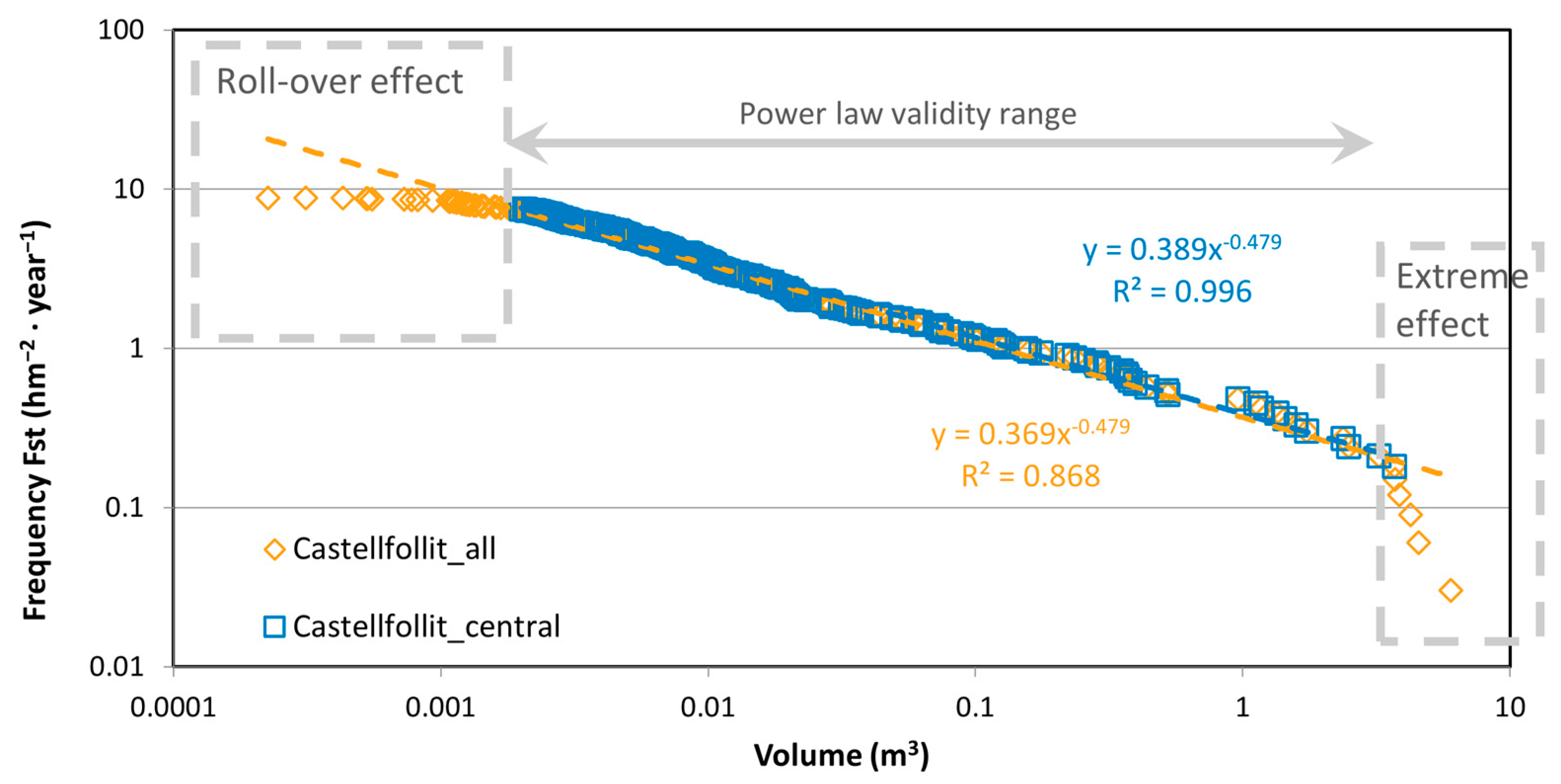
4.1.1. Rollover Effect

The roll-over effect at the lower limit of landslide inventories has been widely studied for all types of landslides and also for rockfall. This relates to the completeness of inventories and is commonly excluded from analyzes that are focused on magnitudes capable of causing significant damage [72,73,74,75]. In rockfalls detected with TLS monitoring, the lower threshold is small enough to include all the cases of interest. In this sense, we will only make a theoretical reflection on the conditioning factors in the roll-over effect in our application cases. It is necessary to consider the possibility that, physically, the massif would have a lower limit of volume susceptible to detachment conditioned by the failure mechanisms or the degradation of the rock. In Montserrat, the rock mass is formed by a conglomerate, according to the mechanism m e c 3 of detachment presented and discussed in Section 5.2.3, which corresponds to the weathering of the rock matrix and the fall of isolated pebbles. Detached volumes up to 10−6 m3 are physically possible and abundant around 10−4 m3. Beyond these actual lower limits, a roll-over effect can be caused by undersampling the smaller volumes. First, the performance of the laser scanner equipment and its on-site implementation determine an instrumental limitation to capturing small detachments. It is influenced by the measurement precision, the visual distance, the visibility of the rock surface, and ultimately the density of points obtained as a result of all the previous factors. Likewise, post-processing adds some additional restrictions, according to the criteria for defining clusters of points as detectable entities and the methods of discrimination and validation of results. As a result, in our case sites, this threshold for roll-over effect can be placed commonly in the range of 1 · 10 3 V m i n 5 · 10 3   m 3 . Finally, there may also be limitations derived from time discontinuities in data capture. It could be the case that changes detected throughout the period between surveys have actually been different falls, but due to being adjacent, they are confused into a single major one. This restriction could hide processes of progressive rupture that are very important to risk management [76]. These considerations link to those made in Section 2.2 for surveying design.
To identify the threshold at which this roll-over effect is noticeable in the sample, an empirical method is applied equivalent to the considerations made by other authors [48,77], which are simpler than those presented by [21]. We use a progressive cut on the sample, starting from the minimum volume and increasing the sense to find the point where the potential fitting is stable. If the sample is sufficiently wide in volume range and sufficiently densely populated, a stretch of stability for the fitting parameters is observed until reaching the point where the sample is already reduced to the right branch and this stability is lost again due to the variability of the upper extreme values. Figure 7 shows the example of the Castellfollit merged sample already presented, containing 298 rockfall events detected in the volume range of 2 × 10⁻⁴ to 6 m3. By applying this empirical method, we determine an upper threshold of the roll-over at 2 × 10⁻³ m3, in which the value’s stability of the parameters is reached for A s t = 0.32 and B = 0.52 , a maximum of the regression coefficient R 2 = 0.98 as well, and the removal of data is still limited (16%).

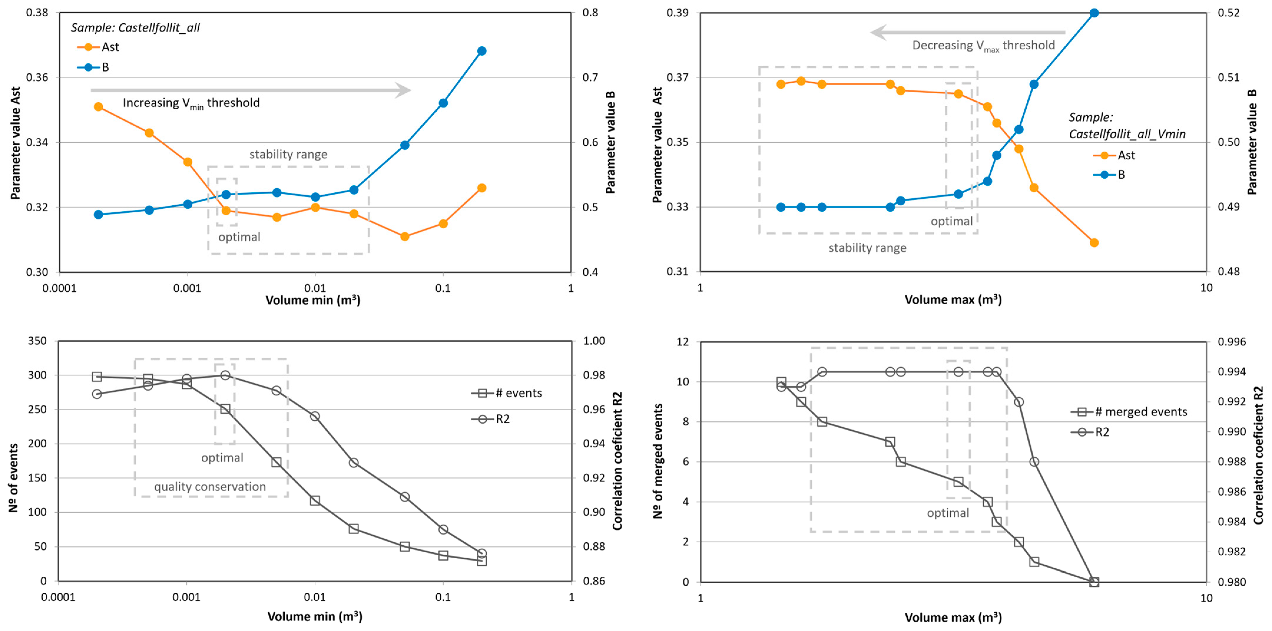
4.1.2. Undersampling of Large Events

This section continues with the same example case of Castellfollit from the previous subsection, once the lower limit for volume was applied. Considering its sample extent S E = 33.14 hm2·year, the largest volume that would nominally correspond to having been observed once in the mean ( F = 1 ) is that of F s t = F / S E , which is V 93 m3. Identically, according to the available S E and the fitted McF, it would be expected to have observed 2 events ( F = 2 ) of V 25 m3, or 3 of V 11 m3. However, the largest volume detected by TLS is 6m3. The shape of the upper limit in the volume distribution in Figure 6 would seem to indicate that there is a physical limit that makes events greater than 10 m3 very unlikely, following the considerations in [49]. Since 1976, however, a maximum detachment of 1500 m3 and up to 7 rockfalls of V 50 m3 have been observed, indicating that this is not the case. This information is available in Supplementary Material SM3. They are only included in the observational inventory because they were there before the start of monitoring with TLS or in places outside of TLS coverage, as was the case with the southern cliff next to the Toronell River in 2011.
On the contrary, we have detected 14 rockfalls in the 1–6 m3 range until 2020, when the fitted McF would expect to have only 6 events within this class. Therefore, we conclude that in our sample we have an undersampling of the largest volumes, in the sense that major events have accumulated in similar values of volume instead of differentiating more in gradation. Another effect could also be present, according to [77], due to the temporal spacing of the monitoring surveys or the criteria in the delimitation of the detached rock blocks, since these volumes actually represent multiple events interpreted as single events. In any case, such a distortion in the extreme values leads to a mismatch in the regression of the potential law. In this upper range of major events, the most significant fact is their occurrence, not so much their specific volume. In this sense, we can apply a filter to optimize the adjustment of the potential law. By comparing observed F ( V i ) with theoretical F s t ( V i ) · S E , we identify the major events with the largest divergence to be filtered manually. However, it is not an elimination of their occurrence, as far as the following data maintains the cumulative frequency.
Alternatively, we can apply the empirical method analogous to that of the preceding subsection for roll-over. In this case, we are trimming the sample by progressively discarding one record in a decreasing sense from the maximum volume. Using the Castellfollit example once more, Figure 7 demonstrates that the adjustment parameters attain stable values rapidly, where we select the optimal point with a maximum regression coefficient R 2 = 0.994 for A s t = 0.365 and B = 0.492 . This filter to V = 3.3 m3 instead of 6.0 m3, which was the largest detected rockfall, corresponds to collapsing the five largest registers into the sixth one. This maintains the value F = 6 as real cumulative frequency.

4.1.3. Oversampling of Large Events

The variability in extreme values argued in the previous subsection can also occur in the opposite direction. A clear example of this is the Degotalls north sub-sample. On 2nd January 2007, a 300 m3 rockfall on this 180 m high wall caused severe material damage to the monastery parking lot and the rack railway that runs parallel 115 m further down the slope. The recovery work included intensive rock clearing and fence installation, as well as the removal of parking spaces, while the next phases of protection were planned, including a project to stabilize large, potentially unstable blocks in the wall. In support of these tasks, the first laser scan of the wall was carried out in May 2007. Before starting this second phase of work, the progression of the rupture produced a new detachment three times larger on 28th December 2008, which forced the reconstruction of protective fences and stabilization, including their extension to cover both walls (N and E). These events have led the following TLS monitoring series to include a period of exceptional activity from 2007 to 2009.
Figure 8 shows the TLS records of activity on the Degotalls wall (north and east merged) and their McF distribution for the period 2007–2009. This includes the large detachment in 2008 and much of the clearing and stabilization work conducted on the wall. Figure 8 also shows the period 2009–2020, with S E 2007 09 = 7.98   h m 2 · y e a r and S E 2009 20 = 33.48   h m 2 · y e a r , respectively. For the total sample extent S E = 41.47   h m 2 · year once the roll-over has been filtered and McF adjusted with A s t = 0.354   h m 2 · year 1 and B = 0.544 , the largest expected detachment would be of volume V = 140   m 3 , which corresponds to F = F s t · S E = 1 . However, due to the described circumstances, the monitoring period has coincided with an event of V 1 = 786   m 3 140   m 3 according to the original cubication, which was subsequently revised upwards (see Section 5.2.2). However, in any case, the event was much greater than expected. This is not the case for the second sample value, which corresponds to F = F s t ( V 2 ) · S E = 1.6 ~ 2 . Equivalently to the treatment in the preceding subsection, the first value is not considered, but its occurrence and successive cumulative frequency values are. Once the effects of the two extremes, upper and lower, have been filtered, an optimal adjustment of A s t = 0.339   h m 2 · year 1 and B = 0.555 with R 2 = 0.991 results in a range of validity for almost 5 orders of magnitude in volume.

4.2. Observational Data Analysis

A basic property of the observational inventory is that it samples only if “seen” (a human view of the phenomenon) or “noticed” (damages and effects). Therefore, the detection capacity depends on the human presence and, by extension, their exposure. Consequently, the first question that arises is about the completeness of the sample that we can obtain, as already pointed out in Section 2.2. This leads to epistemic uncertainty, as discussed in [78]. This section starts with the question: Have we recorded all the activity (for all sizes) throughout all the time and covered all the space from which the inventory is obtained? Additionally, since the answer is negative, we attempt to solve the inverse question: of what space, of what period, and for what range of volumes is the obtained sample in the inventory representative?
As seen in Section 4.1, the detection of detachment activity with TLS enables a complete sample within its full extent S E to be obtained homogeneously for all volumes within a central range. S E of the sample is an attribute derived from the design of the monitoring surveys due to the start and end dates and their visual coverage. This fact allows direct exploitation of the record and the calculation of McF with a unique and constant S E for the whole sample. On the contrary, in observational inventories, S E is not previously defined but is a deduction from the sample and data it has been possible to collect in the past. In this case, we identify that the sample is heterogeneous since S E ( V i ) depends on the volume range. The strategy proposed in this case and presented in the following subsections consists of segmenting homogeneous sub-samples so that they can be calculated in terms of F s t and then integrating them again into a wider sample. To accomplish this, if sub-samples are discretized on the same basis as uniform categories of volumes, the subsequent integration is facilitated. In this work, the half-decimal order of magnitude is applied to get a uniform distribution on the logarithmic axis. McF undergoes a slight variation between continuous and discrete samples, as represented in the subsections below.

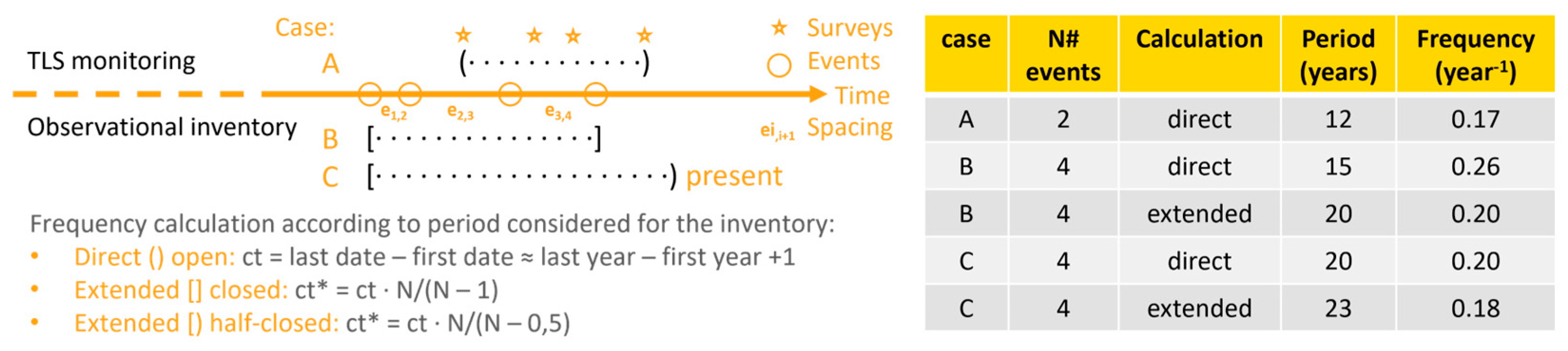
4.2.1. Frequency Calculation on Inventories

Spatio–temporal frequency is simply calculated as F s t V = N ( V ) / S E , N ( V ) is the number of events with a volume greater than or equal to V and S E includes the period c t of temporal coverage of the sample and the surface of the source area c a , according to Section 2.2. This has been conducted with the TLS monitoring data, in which the period directly obtained by the duration of the campaigns c t = t n t 0 is considered, with t 0 being the date of the first survey and t n being the date of the last available, which we know precisely by day and even by the hour. If we bypass the spatial normalization to focus on the temporal frequency, we have that F t V = N ( V ) / c t . In contrast, for observational inventories, there are two considerations to be made, as shown in Figure 9. On the one hand, in historical data, the dates are often imprecise, and we treat them only with the resolution of one year. In this rounding, we consider that the entire calendar year in which an event is located is covered by the inventory record, given that it has been covered by the effort to recover data from past activity. In this case, the period is calculated directly as c t = l a s t   y e a r f i r s t   y e a r + 1 . In addition, as stated in the previous paragraphs, in the records of observational inventory there is an indeterminacy in the time period covered by the sample obtained, especially when the observation has been indirect (e.g., historical documents, survey). If we consider that the period covered c t by the sample is delimited by the first and last observations, we would incur an overestimation of this frequency, since intuitively it must correspond to the inverse of their average spacing e ^ = i = 1 N 1 e i , i + 1 / N 1 = c t / ( N 1 ) , where e i , i + 1 is the spacing between each event and the next one.
Consequently, it is appropriate to consider an extended period c t * that corrects this distortion and becomes truly representative of the events in the sample. This allows the calculation equivalent to the monitoring data, F t V = N ( V ) / c t * and equivalently, F s t V = N ( V ) / S E * in the cases shown in Figure 9. There, we represent an open interval when both endpoints of the period are defined independently of the sample, as is the case for TLS. On the other hand, a closed interval corresponds to a period fitted by the first and last recorded event and then c t * = c t · N / N 1 . Finally, a half-closed interval is used to represent the most common case in historical inventories, in which the period is set between the first record in the past and present time and the period should be extended by the half c t * = c t · N / N 0.5 due to the initial extreme fitted by sampled data.
Since in observational inventories it is common to have few observations, this distortion can be relevant, although it loses weight as the value of N grows. This correction of the extended period c t * will gain influence in the analysis presented in the next subsection, where different periods are considered for each volume class. For example, in Castellfollit de la Roca, the historical inventory collected five recent events larger than 10 m3 in the last 30 years (1995, 2007, 2011, 2015, and 2017) (Figure 10). The closed interval defined by these events is c t = 2017 1995 + 1 = 23   years and the corresponding extended period c t * = c t · N / N 1 = 28.8   years . If we consider the half-closed interval between the first event and the present time at the end of 2020 included in the analysis, c t = 2020 1995 + 1 = 26   years and the corresponding extended period c t * = c t · N / N 0.5 = 28.9   years .
In conclusion, the time–frequency calculation is subject to uncertainty [79], especially in the range of the largest rockfalls, where the number of records is very low, reaching the extreme case of a single observation, for which the idea of recurrence loses its meaning and c t * falls into indeterminacy. Accordingly, when considering c t * , the volume range where a single event is recorded may not be considered sampled enough to be included for the McF adjustment.

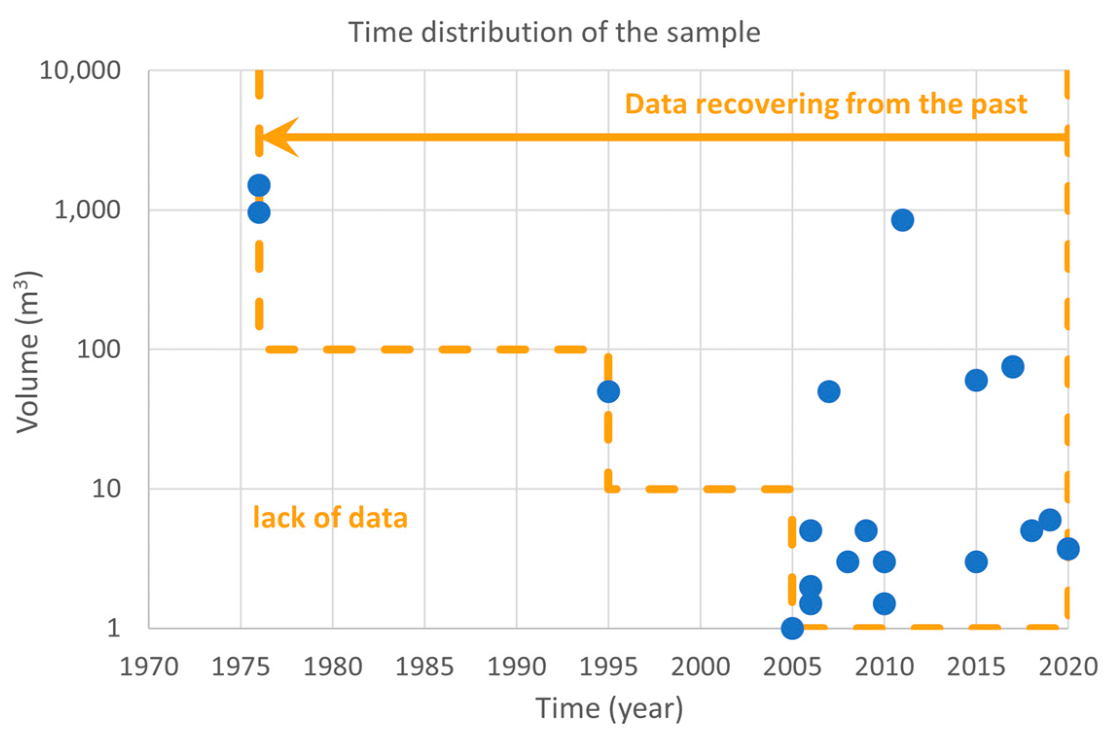
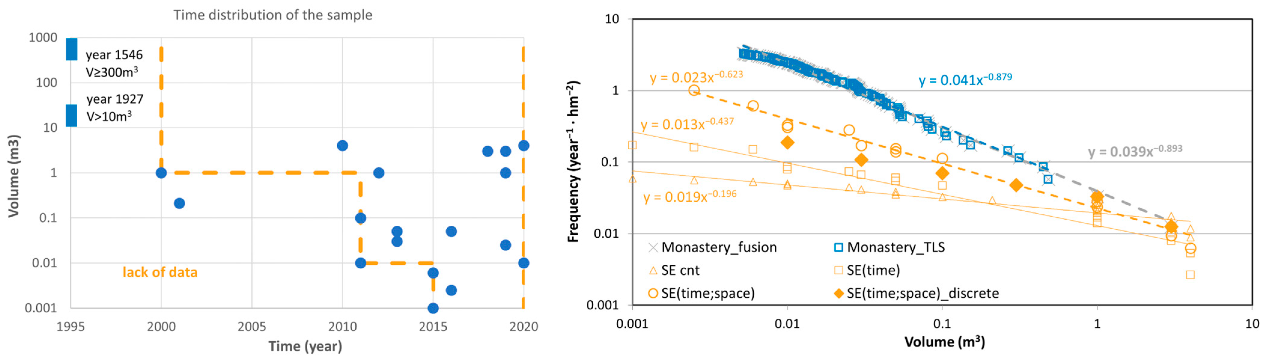
4.2.2. Size Distribution of Registered Events over Time

In the analysis of rockfall inventories, it is revealing to visualize the temporal distribution of the records collected. For example, Figure 10 shows the 19 events of the historical inventory in Castellfollit de la Roca collected in 2020 when searching for antecedents. On this distribution, we identify the volume ranges in which we have a sufficiently homogeneous sampling: during the 16 years of the period 2005–2020, we have a representative sample of rockfall with V   1 m 3 ; during 26 years from 1995 to 2020 we have a proper sub-sample of V 10   m 3 ; in 45 years of the entire period 1976–2020, we can only characterize the sub-sample of V 100   m 3 . In the bottom-left margin of the graphic, we identify a data gap in the inventory. In contrast, TLS monitoring detected 15 rockfalls inside the range of 1   m 3 < V < 10   m 3 detached from only half the cliff for 13 years ( S E = 33 ). It must be supposed that from 1976 to 2005 there was some V < 10   m 3 rockfall activity, but this information has not remained as a dated record in the memories of the interviewees nor in the available documentation. It should be noted that the definition of these sample limits is quite interpretive, with a margin of variability depending on the analyst.
This treatment corresponds to considering a variable value of c t and S E also in F s t calculation. In Figure 11, several McF adjustments can be observed and compared under different hypotheses and formats. Firstly, if a uniform c t = 2020 1976 + 1 = 45   years was applied to the whole range of volume values, A s t = 0.097 and B = 0.335 would be obtained. This means that for every 10 rockfalls of V 1   m 3 , one of them has V 1000   m 3 , because this low value of B implies that every three orders of magnitude in volume correspond only to one order of magnitude in frequency. Secondly, if a variable value of c t is considere a function of volume range, according to the considerations of lack of data in Figure 11, the slope of the regression line increases significantly to values B ~ 0.5 . Additionally, A s t arises because F s t is maintained for the largest rockfalls and is increased inversely to the c t value for successively smaller rockfalls. In this case, a slight difference is obtained between both considerations of covered time, either direct c t or extended c t * . The slope increases a little bit, being the fixed point in the lowest volumes where the c t * c t , as N 1 . Finally, the result is shown for the case where a discrete scheme is used for the volume. In this case, groups of data collapse at the beginning of their volume class, for instance: four rockfalls with a volume of 30   m 3 V < 100   m 3 compute for the class V 30   m 3 , at a lower value of volume. With a negative slope, this implies a slight lowering of F s t values for infrequent events and an additional increase in the slope B .

4.2.3. Size Distribution of Registered Events over Space

Finally, we address one last issue that affects inventory samples. It is relevant to remember the big difference between monitoring with TLS, which makes an exhaustive detection in the starting zone by a repetitive, systematic process, and inventory. This leads to observations in the arrival zone, often only in a reactive way to events with effects, which are conditioned by the propagation of falling rocks down the slope. The smaller the magnitude, the more conditioned the observation is on the fact of producing damage or effects to the elements at risk. In most inventories, the elements at risk act as data collectors, and their exposure and vulnerability somehow determine their detection capacity. Therefore, the position of the elements at risk concerning the extent of the rockfall trajectories is very influential in the sampling. When the inventory is built based on photointerpretation, despite not depending on the presence of human elements, it similarly happens that the detection capacity is conditioned by the rockfall propagation and the imprint generated on the environment, for example on the forest. This approach is similar to the idea of an “effective surveyed area”, which was introduced by [73] in inventories for landslide susceptibility analyses.
In the previous point, we asked ourselves, “What time span have we effectively controlled with the tasks furnishing the inventory?” Here we ask similarly: what space have we effectively controlled? Furthermore, equivalently to the answer to the first question regarding time, we find again a dependence of covered space on magnitude. Focusing on the case of Montserrat, we can see very clear examples of this idea. For instance, the built enclosure of the Monastery is surrounded by vertical walls, at the foot of which there are buildings and occupied spaces. Any event, even one of a small magnitude, can already have an impact on human activity and be perceived and recorded in the inventory. On the other hand, continuing up the slope, there are other more remote outcrops. If rocks fall from these, even if they are bigger than the previous ones, they are retained in the forest or the gullies and can go completely unnoticed. This means that the area covered by the sample, which contributes to the S E count, is variable according to the volume range. We can apply this distinction based on the division of the Montserrat massif into domains introduced in Section 3.1. In Table 4 and Figure 12, it can be seen that the application of this idea to the Monastery sample can be quantified, although based on expert judgment. Thus, for example, a rockfall of 1 m3 is only recorded if it occurs at lower levels, while an event of 100 m3 will be recorded anyway due to its visibility and repercussions.
This consideration generally implies an increasing value of S E with magnitude. However, at the highest extreme of magnitude, another consideration is also possible: can a rockfall of enormous magnitude occur at any outcrop of the rocky massif? As several authors have proposed [7,14,49,80], each rocky outcrop has a physical limit to the magnitude of events that can occur. This depends on the structure of the massif (mainly joint persistence) and the intersection with the surface of the escarpment, as well as its extension and especially its height. In this sense, we can identify some domains where the conditions are not met to generate failures greater than 3 × 10³ m3 or 1 × 10⁴ m3 (see Table 4). In the available inventory, we do not have any cases of this magnitude, so this effect does not influence the present analysis.
If we proceed with the case already presented by the Monastery of Montserrat, once this correction is applied to the McF adjustment, its influence on the parameters is evident. Here, the inventory collects 20 rockfalls with a total extension of 15.7 hm2 of rock walls, two of which are ancient and considered outside the continuity of registration. Both are well dated: one in 1546 has been obtained by documentary source, and the other by survey, and thanks to registration in a memorial, we know that it occurred on 19 May 1927. Since we lack information on the rockfalls themselves, we only know how they influence the surrounding landscape. This makes it difficult to estimate the volume, which is assumed to be equal to or greater than 300 m3 and clearly greater than 10 m3 respectively. Thus, we are considered to have only a sample suitable for McF analysis for lower volumes (Figure 13). If a uniform S E is applied to the entire sample resulting from 18 rockfalls in 21 years, the slope of the McF curve is very low ( B = 0.20 ), which is equivalent to saying that the probability of occurrence is quite similar for any size. Considering the correction described in the previous section, which makes S E variable over time and leads us to discard another set of data outside the confidence margin in the sampling, parameter B already takes a value greater than double ( B = 0.44 ). Moreover, if we consider the spatial variability of S E that is presented in this section, according to the values in Table 4, the slope ( B = 0.64 ) is already assimilated to other values in Montserrat for other sectors, although it is still significantly lower than what TLS monitoring indicates ( B = 0.88 ) for the local Monastery station placed at Fra Garí viewpoint.
Given the results, we conclude that the inventory achieves sample completeness for V 1   m 3 , but smaller rockfalls, it is sure to have missing records due to a lack of systematicity in data capture. This makes the adjustment fall short compared to the TLS monitoring for the range of 1 × 10⁻³ to 1 × 10⁻¹ m3, which covers a fairly similar time span. It should be noted that there are five major rockfalls in the inventory dated within the monitored period by TLS. However, they have not occurred in the space covered by the TLS surveys (3.57 hm2), which is 38% of the 9.4 hm2 that we consider covered by inventory at this range of volumes. Consequently, we see a high complementarity of inventory with monitoring, as we will detail in Section 5.1. In this case, it allows us to have confidence in the extrapolation of the TLS McF adjustment up to around V = 10   m 3 . Therefore, it is assumed that S E of TLS monitoring is large enough in time and space to reach a representativeness similar to the inventory, thanks to its completeness. The treatment discussed in this section has a significant impact on the McF adjustment for the rack railway industry. This is due to the fact that the position of the rack railway relative to the cliffs and rockfall runout varies along its route. More details on this sample can be found in Supplementary Material SM5.
In this work, the corrections have been applied to covered time and space depending on the volume in a coupled way, that is, for a certain magnitude range, a limitation of the time covered by the inventory is applied everywhere and a space restriction in sampling applies at all time spans. A possible extension and generalization of the method would consist of decoupling both variables and being able to determine the spatial–temporal coverage of the inventory independently. For each range of volumes in each domain, consider the period of time covered by the inventory. Even the temporal coverage could not be unique until the present but could be discontinuous when the available inventory is very heterogeneous as a result of work in disjointed stages.

5. McF Discussion

Both case sites (Montserrat Massif and Castellfollit de la Roca) and both data sources (TLS monitoring and observational inventory) were analyzed using the methods described in Section 4. Results for Montserrat are collected in Table 5 and Table 6, and for Castellfollit in Table 7. In the present section, results are discussed, focusing on different points of interest in each subsection.

5.1. Spatial Variability in McF

We have obtained the McF relationship that can be considered best adjusted to each available sample at different scales: outcrop covered by a TLS station, sector by a grouping of nearby TLS stations, or by areas covered by homogeneous inventory, and the massif as a whole.

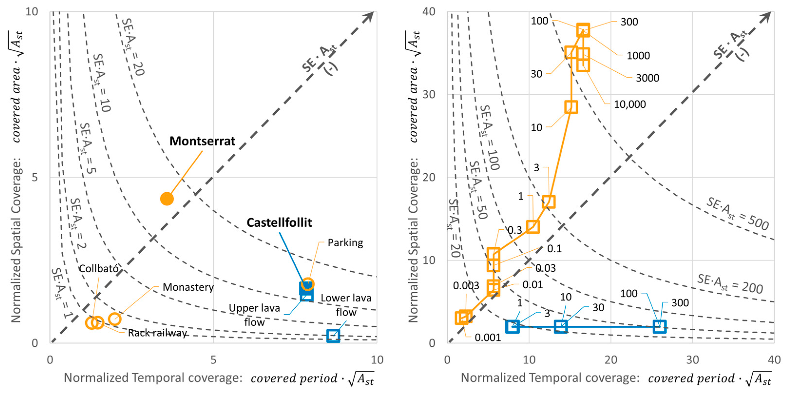
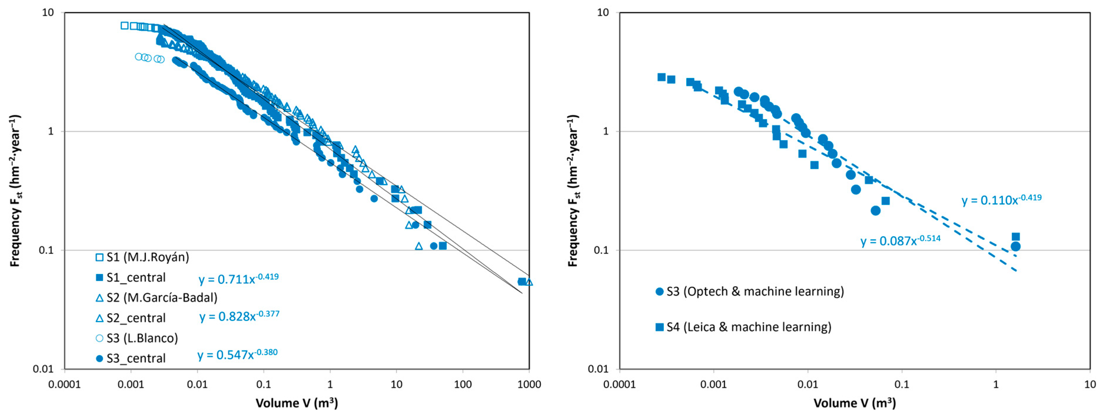
5.1.1. Multi-Scale Comparison

In the results from TLS in Montserrat (Table 5), we observe a large variation in McF laws comparing all the stations: A s t ranges from 0.04 to 0.6, and B ranges from 0.45 to 0.88. When we group the samples into regions, disparities are reduced, and each behavior can be attributed to different conditions over the mountain: upper/lower levels and north/south flanks. These regions are: Monastery (single station) is an upper-south slope; Parking (merging Degotalls north and east) is an upper-north slope; Railway (merging Guilleumes and Sant Benet) is a lower-north slope; and Collbató (merging Collbató road and Can Jorba) is a lower-south slope. These regions are equivalent to those obtained by the inventory analysis (Table 6). There are significant differences between McF provided by TLS and inventory (Figure 14), as will be discussed below. When regions are combined into a single McF for the massif as a whole, both sets of results are the same. Then, we obtain the coincident value for B = 0.62 and the value for A s t = 0.16 from TLS is more confident than the derived from inventory, which is seven times lower due to the incompleteness of the sample that is not achieved to offset. In any case, Montserrat is a rocky mountain with many conglomerate walls of varying slope, aspect, and height, so any McF result for the massif can only be intended as an approach to the average trend, for which it should be expected to have large spatial dispersion.
The results of the inventory analysis are presented in Table 6. McF parameters were obtained for each sub-sample of an inventory region according to the methodologies presented in Section 4.2. Optimal fitting was found through the analysis that applies the extended period c t * to the continuous sample and consider the variable value of S E ( V ) with magnitude according to the time and domain of each registered event. In contrast to homogeneous samples of TLS with constant value S E , where the merge can be conducted directly by mixing all data and adding S E , in inventory samples, it is proposed to discretize the samples on magnitude classes to be able to apply the equivalent procedure. In that case, direct period c t is used to calculate frequencies because we expect the event count to increase in the merged sample. It is worth noting that regions where any major rockfall was observed also contribute to adding S E for the largest events. In other words, the absence of recorded events of large magnitude in a sample of inventory is also data to be considered for a proper calculation of their frequency when merged with other regions where this kind of event was observed. This point agrees with considerations made for TLS monitoring in Degotall’s north wall that include an exceptionally large event (see Section 4.1). To improve the frequency calculation of the largest events, a sub-sample without correspondence to the TLS monitoring station (northern road in Table 6) has been added to the sample. This way we collected two rockfalls with V 1000   m 3 detected over S E = 4978   h m 2 · y e a r .
In contrast, for Castellfollit de la Roca (Table 7), differences between TLS and inventory are reduced (see Figure 14). In this site, we consider a single region because the extension of the basaltic cliff is reduced, but two analyses of spatial variability were attempted. It could be distinguished between north and south flanks corresponding to each fluvial valley using inventory data, although samples are very poor (9 and 10 events each). McF differs from the north flank ( A s t 0.15 and B 0.33 ) to the south flank ( A s t 0.4 and B 0.6 ), which agrees with the observation that larger rockfalls seem more frequent at the higher north cliff, while rockfalls of V 50   m 3 would have a similar frequency in both flanks. TLS stations cover different parts of the cliff: the station in river parking is focused on the lower lava flow forming the cliff (as explained in Section 3.2), and the other two stations are focused on the upper lava flow. These results (shown in Table 7 and Figure 14) indicate that the lower level has the higher activity of lower magnitude than the upper level, which agrees with the observation of upward erosion that configures the overhang profile of the cliff and leads to larger failures in the central-upper part. However, the sample attributed to the lower level has the smallest S E value, it watches to the end extreme of the cliff, and it covers a scar from the large event that occurred in 2011, so it may reflect other factors modulating rockfall activity. In Supplementary Material SM4, it is highlighted that maps or location figures of the inventoried activity are not necessarily indicative of the hazard distribution within the wall but must be interpreted according to the cycles of activity that may manifest.
Similarly to both lava flow levels at the cliff in Castellfollit, at Degotalls Wall in Montserrat, slight differences in rockfall activity are seen according to stratigraphic levels in the same outcrop. The rock mass shows smaller values of joint spacing in the lower half of the wall compared to the upper half, and correspondingly higher activity is detected in the lower part. However, these results are affected by the artefacts analyzed in Section 5.2.2, preventing them from being conclusive. Nevertheless, this variability has been observed at other sites [50] and is fully consistent with the model and methods.

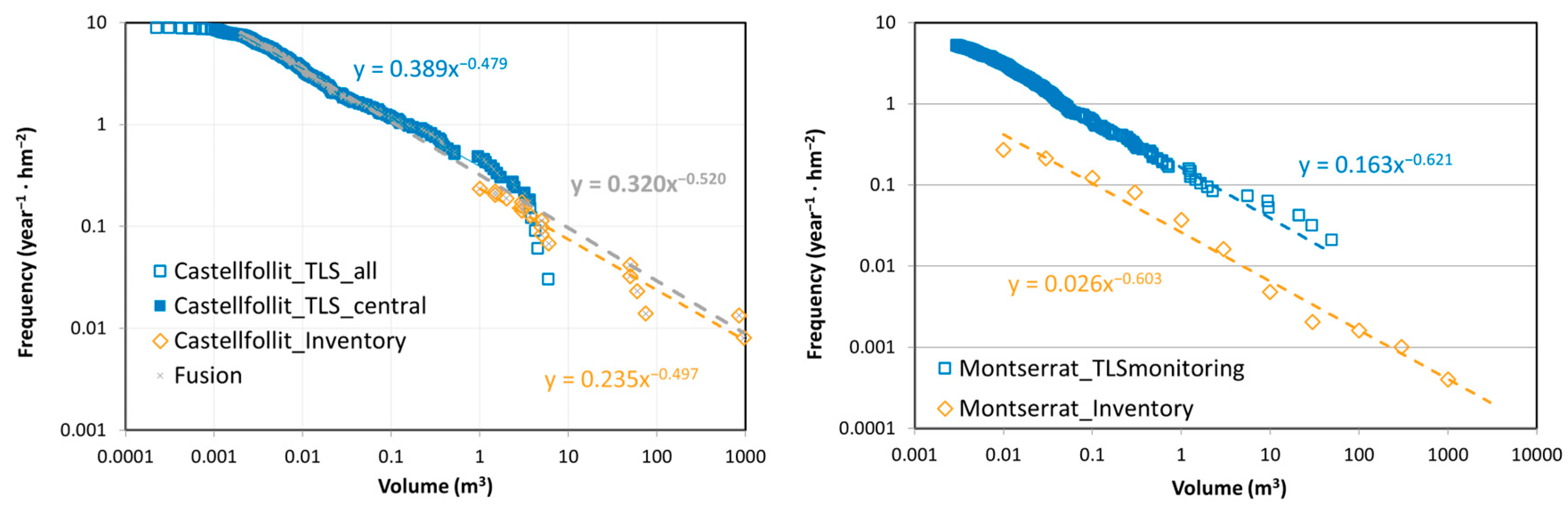
5.1.2. Multi-Source Comparison

As seen in Figure 14, McF results derived from TLS monitoring and observational inventory differ. In Castellfollit de la Roca, this difference is small, and both McF can be attempted to be merged into a fusion sample (see Figure 15) to get validity on the maximum range of magnitudes and be confident on the hazard scenarios at any point of the McF curve It has already been demonstrated [81] that there is a similar degree of coherence in Yosemite (USA) between rockfall inventory and remote sensing detection (combined TLS and SfM applied to aerial and terrestrial images), thanks to the high-quality inventory available [82]. In Montserrat, A s t obtained by inventory is six times lower than the value from TLS. We conclude that the inventory lacks quality and is insufficiently systematic to overcome the high variability present in Montserrat. However, similarity in both values for B gives us confidence to extend McF resulting from TLS two orders of magnitude up to major observed rockfalls ( V < 10 4   m 3 ).
We conclude a large margin of complementarity between both data sources, which could still be expanded with others of those presented in Section 1.2. On the one hand, TLS provides systematic detection that is homogeneous for all magnitudes, leading to a complete sample. Attention must be paid to S E value because it tends to have very local and short monitoring that limits its representativeness. Finally, new studies can only be planned from the present to the future, forcing them to wait a certain amount of time for a sufficient sample to be built. On the other hand, inventory allows going back to the past as long as there are preservation sources of activity data (e.g., written, oral, graphic). It can also cover a large sample size in both space and time, but there is no longer homogeneity with magnitude, and its completeness must always be questioned.

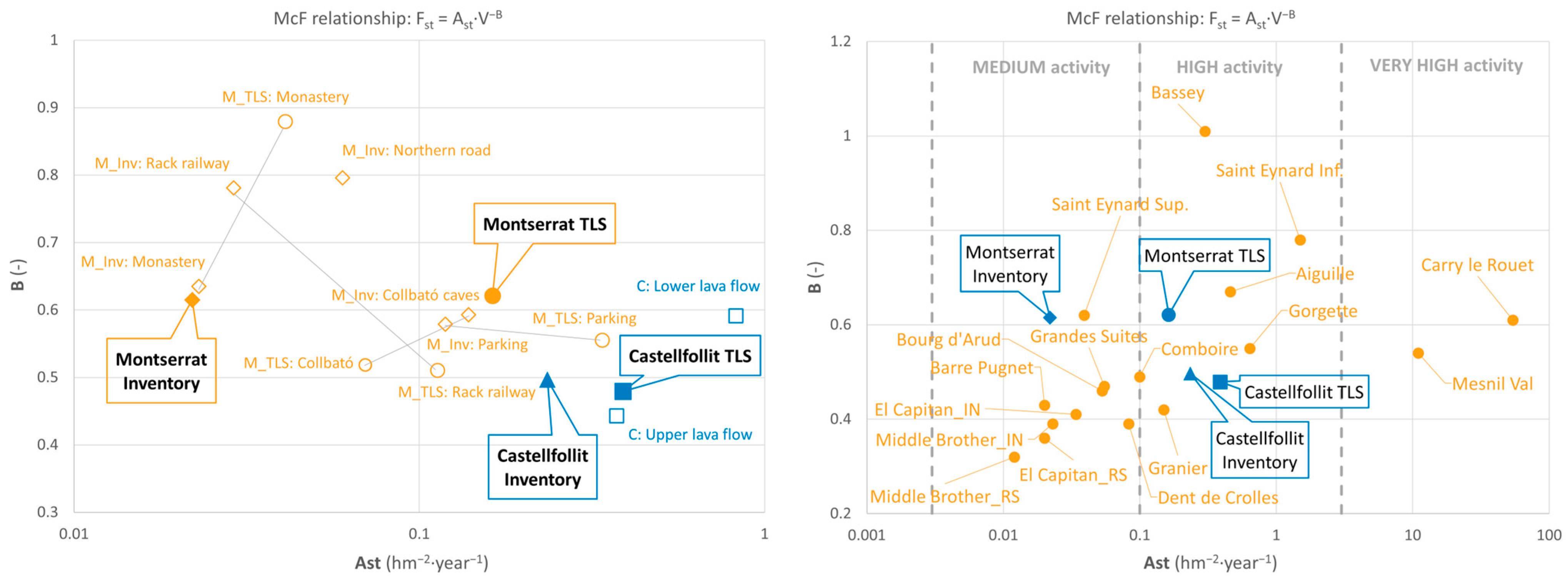
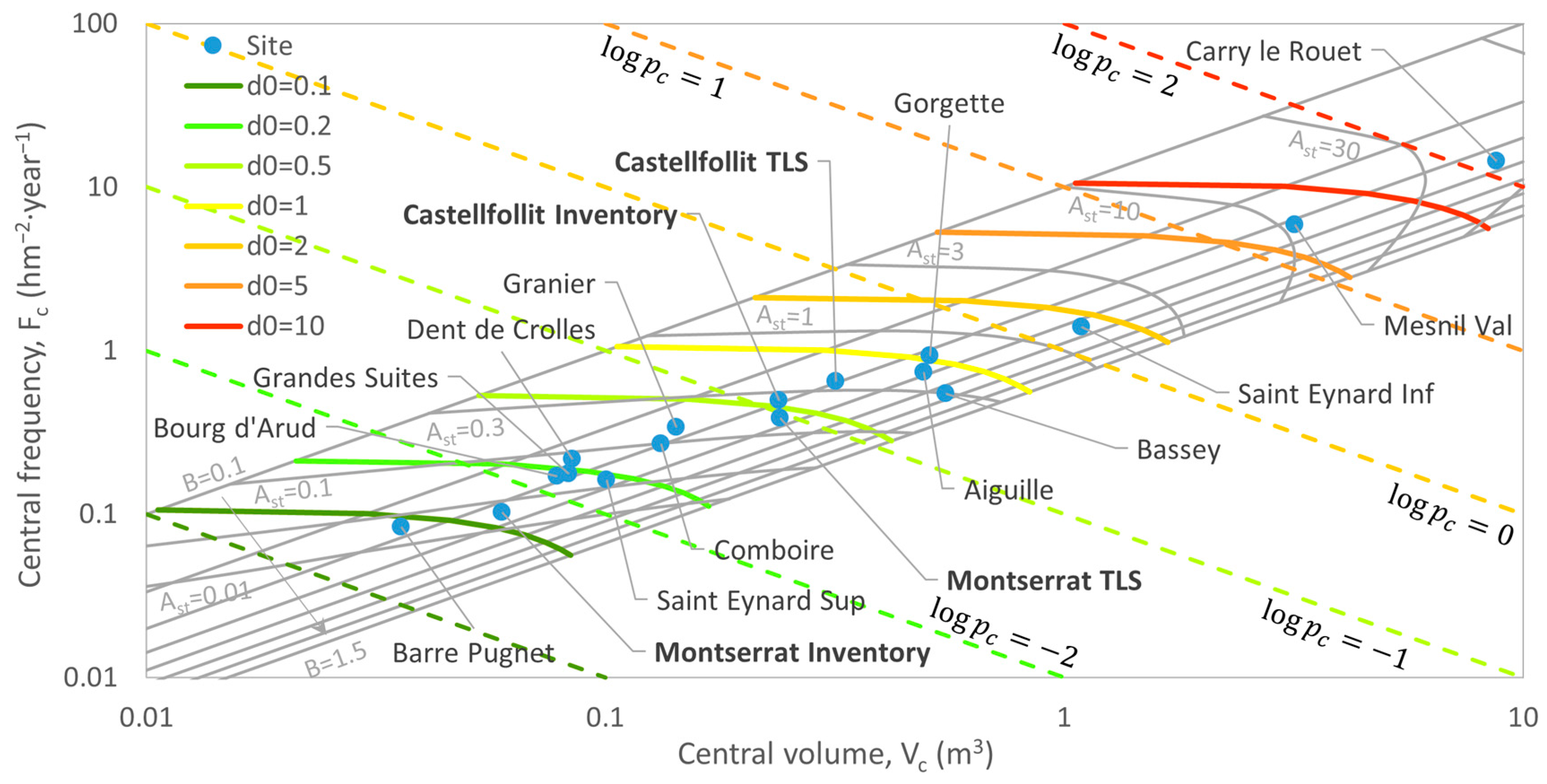
5.1.3. Multi-Site Comparison

In Figure 14, McF values for Montserrat and Castellfollit are compared to other reference sites in France and Yosemite, USA [7,81], and agreement is observed. According to these previous references and present results, the following conclusions are drawn. Parameter B is related to rock mass structure, and its value increases as the interlocking of the rock pieces decreases, which is related to the joint’s pattern and strength. The alternation of soft and hard layers could produce an additional increase in B . Parameter A s t is related to the geodynamical context and the intensity and constancy of erosive and triggering actions. For instance, it is expected highest to the lowest value of A s t when moving from coastal cliffs or deglaciated valleys to riverside slopes or mountains in a temperate climate. Thus, it is suggested to distinguish degrees of rockfall activity according to A s t (see Figure 14). The scale step factor used a one and a half decimal order of magnitude to keep similarity to the frequency classes adopted by the Austrian norm ONR-24810 [83] to define nominal blocks for rockfall fence design.
This comparison of different sites is difficult to read in terms of hazard, due to the dispersion in the plane of both parameters A s t and B . As stated, it is quite clear that an increase in the value of normalized activity A s t is directly related to a greater hazard, but the influence of parameter B in terms of hazard is less clear. When the value of B differs between two cases, it is difficult to directly compare McF curves. For this purpose, it would be useful to know the center of the hyperbola V c ; F c defined in Section 2.1, which represents McF in a single point (see Figure 16). On this plane, p c and d 0 are suggested as proxy descriptors of intrinsic hazard, which means, all conditions of the rock mass (e.g., structure, geotechnical properties) and environmental context (e.g., climatic, seismic) influence the hazard before the slope geomorphology itself. Features of the outcrop (e.g., height, slope, aspect) will modulate this intrinsic hazard to the complete idea of rockfall detachment hazard when the area below the McF curve is integrated with the range of expected magnitudes V m i n ; V m a x according to [7].

5.2. Temporal Variability in McF

A direct reading of the rockfall activity as the total number of events per year or the corresponding rockfall total volume rate m 3 / y e a r is not sufficient to assess a possible evolution of the hazard. Obviously, in one period there may be more activity of a lower magnitude compared to another of the same duration in which a single major event occurs, and the reading in terms of hazards may be different depending on the magnitude-frequency balance.

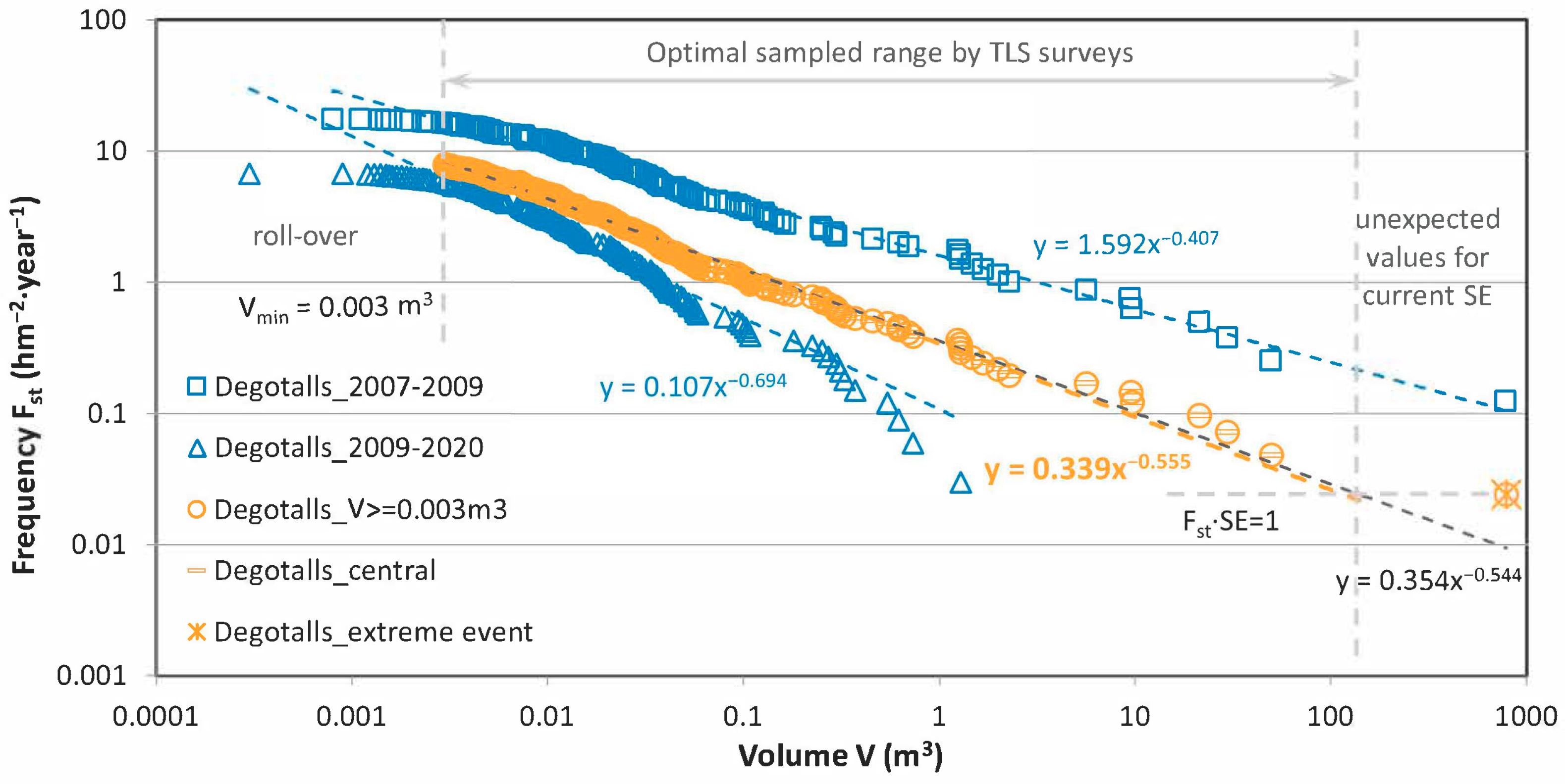
5.2.1. McF Relationship over Time

Taking the longest series of Montserrat (Degotalls and Monastery), an analysis of the variability of McF has been completed over the years. Sub-samples have been taken for periods ranging from one to two years, depending on the availability of surveys and the data obtained. Figure 17 shows the variability of the parameters A s t and B in the adjustment for each period in the raw data, avoiding filtering extreme effects explained in Section 4.1 to keep the entire sample. In the walls of Degotalls (N and E treated together to have wider sub-samples), the initial period corresponding to the great rockfall and subsequent works on the rock face stands out with a much higher activity than the rest, as already seen grouped in Figure 8. In this detail, we see that the value of A s t in the critical period 2007–2009 has no similarity with the rest, which have an average about eight times lower, and this comparison factor raises to 58 between the maximum ( A s t = 1.6 in 2007–2009) and minimum values ( A s t = 0.028 in 2019). Some inverse effect is also observed between the profiles of A s t and B , which is related to the maximum volume detected in each period. In a period when a noticeable event occurs, the value of B decreases and that of A s t increases compared to the general trend. We also observe a global trend of an exponential decrease in activity (number of rockfalls) that can be related to the protective works conducted and perhaps also to the evolution in analysis methodology, criteria, and tools, as reviewed in Section 5.2.2 and Supplementary Material SM5. Figure 17 includes the same analysis for Monastery rockfalls detected by TLS, where the same effect is also present but with less variability.
It must be concluded that rockfall activity and hazards vary over time on this annual or multi-year scale. The available series are not long enough to relate this to large cycles of triggering factors, and the surveys are not frequent enough to search for seasonal variability. Continuous monitoring could provide us with this information about triggers as become successively more common [84], or alternatively adapting survey cadence to triggering factors occurrence such as conducted by [85]. Finally, in both cases, we can see the wide variability of the McF adjustments obtained, a fact that highlights the importance of extending SE sufficiently to be able to obtain representative results of the representative hazards of the place in a timeless way, not conditioned by transitory circumstances.
An important point in this analysis is the representativeness of each sub-sample. In Figure 17, S E of each period is compared with a minimum value S E m i n = 1 / F c that is equivalent to the condition S E u c = S E · F c = 1 as introduced in Section 2.2. Except for the first surveying period in Degotalls (2007–2009), where S E u c 1 , the rest of the periods in Degotalls and Monastery are at the limit of S E u c ~ 1 , so the adjusted values for A s t and B must be taken with caution. The number of data points is also shown, but it is less indicative of the achieved representativeness.
Since rockfalls are not continuous movements but, on the contrary, isolated events of very short duration compared to the long inactive periods between falls, the measurement of the activity is highly dependent on the period of observation, as was seen in the previous section. This variability may reflect many underlying factors as follows [85,86]:
  • Variability of activity is due to natural cycles of the different triggering agents (e.g., rainfall regime, thermal regime, seismic activity, the evolution of the rock massif, and degradation of its resistant properties depending on environmental physical and chemical agents).
  • Modification of the activity due to the work carried out. The clearing of blocks of precarious stability concentrates in a short period a large part of the activity that would have happened more evenly over a longer period. Stabilizing potentially unstable masses makes the future activity less likely in a wide range of sizes. Therefore, McF could provide a quantitative method for assessing the effectiveness of hazard mitigation measures, as explored in Supplementary Material SM5.
In complex cases, such as the wall of Degotall’s north, it is surely a mixture of all these factors. This brings great uncertainty to the definition of hazardous scenarios. In this example of extreme variability, although we take the joint sample of north and east walls and McF adjustments for the 2007–2009 or 2009–2020 periods from Figure 8, we get, on the one hand, an event similar to that of 2008 ( V = 900   m 3 ), which corresponds to an occurrence frequency of F s t = 0.001 to F s t = 0.1 . On the other hand, a detachment hazard scenario with a return period, T = 100   y e a r s , for a unitary wall extension of 1   h m 2 ( F s t = 0.01 ) is equivalent to a rockfall of V = 32   m 3 to V = 2.3 · 10 5   m 3 , practically two orders of magnitude larger than any record in the inventory. This uncertainty would invalidate any further calculation of hazard. Therefore, which is the McF to be taken as a reference? It will surely depend on the time scale of the analysis.

5.2.2. McF Sensitivity to Detection Algorithms

Throughout the sixteen years of TLS applications to rockfall detection at these case sites, methods and tools applied for data processing have been evolving. It can be distinguished four major stages that have given rise to different series of data, particularly in Montserrat, the walls of Degotalls being the most common test area:
  • S1: Classic or standard processing with Polyworks and DBscan tools, initiated by [61] and developed by [62], with data from an Optech TLS device, from 2007 to 2017.
  • S2: Classic or standard processing with M3C2 and DBscan tools developed by [63] and applied by [64], with data from an Optech TLS device, from 2007 to 2017.
  • S3: Machine learning processing with PCM and CC tools developed by [23,67] and applied to data from an Optech TLS device, from 2007 to 2020.
  • S4: Machine learning processing with PCM and CC tools developed by [23,67] and applied to data from a Leica TLS device, from 2018 to 2020.
Monitoring series in Degotalls’ north wall obtained by Optech’s ILRIS-3D TLS device from 2007 to 2017 were initially processed by [62], reviewed by [64], and finally computed by [23] using the developed workflow PCM-CC that uses machine learning for the cluster classification of rockfall candidates. This comparison can be seen in Figure 18. Apparently, the distributions are quite similar, but there is significant variability in the parameters of the McF fit. Changes in criteria are seen in the interpretation of false positives, especially for small volumes. It is assumed that during the first years, there could be a tendency to preventively classify as rockfall the changes with this appearance, even if there was no reliable information to prove it. In 2018, we introduced imagery monitoring in parallel to TLS using the GigaPan device [69] to obtain high-definition images that have been helpful in the process of interpreting the detected changes. At the other end of the graph, for the largest volumes, there are also differences in the interpretation of the blocks successively detached in the period of high activity without intermediate monitoring from 2007 to 2009, which represents significant differences.
Another example of comparison shown in Figure 18 corresponds to the period 2018–2020 when parallel monitoring was conducted using both different TLS devices presented in Table 1. Differences in data capture (e.g., point cloud density, laser footprint) lead to different interpretations despite applying the same analysis procedure (in this case, the machine learning workflow PCM-CC) [23]. Thus, different data capture systems and processing methods introduce variability in results at different stages of the treatment of the point clouds [87], including the uncertainty in the volume calculation of point clouds [71]. This factor has a higher influence in small samples, such as the presented example.

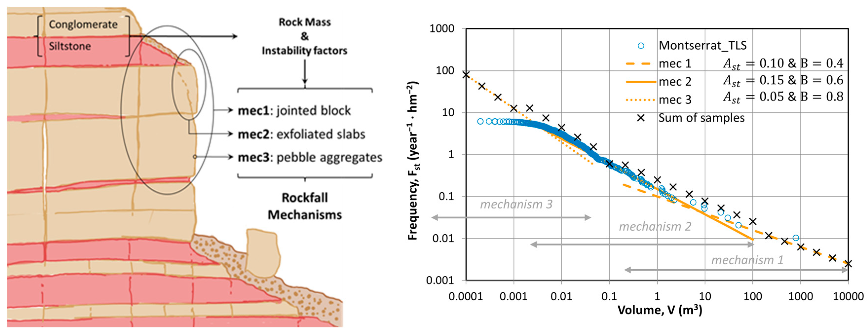
5.2.3. Detachment Mechanisms Overlap

In the McF distribution for the global Montserrat Massif by TLS, a slight ripple shape is observed (Figure 19). Instead of resulting from the previously analyzed specificities in the activity of sites and periods of the sub-samples that make it up, it could also reflect another intrinsic heterogeneity of rockfalls in this massif. As a follow-up to the description of the massif in Section 3.1, three mechanisms of rockfall can be distinguished, according to the structural element that fails and the factors preparing the detachment. They go beyond the classic differentiation (fall-slide-topple) already revealed by [88] that reflects the kinematics of the failure and the first movement when detaching, which have all been observed in Montserrat. Those are related to a range of sizes, but all three classes are overlayed:
  • Mechanism 1 ( m e c 1 ) corresponds to the most considered rockfall type, that is, rock blocks delimited by mechanical discontinuities in the rock mass. For the conglomerates in Montserrat, these are fracture sets and stratigraphic layers, both of high persistence, which delimit prismatic blocks of a wide range of volumes depending on the joint spacing at the specific point, from less than one cubic meter to several thousands of cubic meters (mainly from 10−1 to 104 m3). The basic properties of the discontinuities can be found in Supplementary Material SM3.
  • Mechanism 2 ( m e c 2 ) corresponds to weathering flakes produced by thermal exfoliation, forming curved plates or slabs of intermediate volume from 10−3 to 102 m3, although the most common are in the range of few to several dm3.
  • Mechanism 3 ( m e c 3 ) corresponds to pebble detachment from the conglomerate due to the matrix weathering in contrast to the resistance of the pebbles. Additionally, masses of aggregates can fall together, especially if small and local fractures are present. These rockfalls are of irregular shape and generally of small volume, ranging from 10−6 to less than 10−1 m3.
Since each of these mechanisms responds to different factors of rock mass resistance and destabilizing actions, they could each follow their own McF law over the range of magnitudes they have, which partially overlap. Figure 19 suggests a possible theoretical distinction between the three mechanisms with their parameters ( A s t , B and range of volumes) corresponding to the characteristics observed on the field, which would give rise to a unified McF distribution undulating similarly to that obtained by monitoring.
In this line of work, [23] has begun to apply the distinction of these mechanisms in cluster classification with machine learning techniques. Preliminarily, it has been seen that with the training samples used for the model, a satisfactory classification of m e c 2 rockfalls has been achieved, while lower effectiveness is observed in the identification of the m e c 1 mechanism. This is probably due to the central position of m e c 2 within the sample in contrast to the low number of records of other mechanisms involved in the training phase. Future developments will attempt to achieve a more efficient classification of rockfall clusters, in which the mechanism is also distinguished, and thus be able to confirm if different McF applies and even adapt specific volume calculation formulations to the different morphologies.
In Castellfollit, the toppling mechanism of basaltic columns has been clearly identified, which has led to the detection of precursor movements thanks to its large displacements from [60] to [29] with TLS and photogrammetry. However, lava flows have heterogeneous levels, and there could be other rupture mechanisms as suggested by [60], such as the 2011 large rupture at the fractured base, that may differ slightly in the McF pattern. It will be necessary to deepen it in future studies.

6. Conclusions

The magnitude-cumulated frequency relationship (McF) is the first step in any rockfall hazard analysis, providing the hazard scenarios to be considered in the source area. It is found that McF adjustments are very sensitive to many factors related to the available data (e.g., nature of the data source, quality of the recording, extent and completeness of the sample). The statistical treatment was performed to calculate temporal frequencies. These factors have been analyzed at two different sites, the Montserrat conglomeratic massif and the Castellfollit de la Roca basaltic cliff, where rockfall risk management is an ongoing challenge. Consequently, it has been revealed that it is necessary to carefully identify the attributes of the activity record to know the actual validity of McF over space, time, and magnitude range and what controls its applicability. Uncertainty in both parameters A s t and B in McF laws leads to large indeterminacy when choosing return periods for further risk assessment. We propose to work with the attribute of sampling extent S E defined in Section 2.2 and various ways of expressing the results of McF for better communication of hazards.
In Section 4, a methodological technique for optimizing the utilization of rockfall activity data from remote sensing and traditional inventory is described. On the one hand, monitoring series provide homogeneous samples, which are very useful for the characterization of the central part of the McF curve once the roll-over effect and distortions in extreme values have been filtered, following the indications provided in Section 4.1. Observational inventories, on the other hand, contain sample heterogeneities throughout both space and time since not all magnitude ranges are identified similarly. To fit the available data to the correct ranges of time, space, and magnitude, a processing strategy has been proposed in Section 4.2: inventory is decomposed into homogeneous sub-samples where the frequency calculation is feasible, which are integrated later into a representative joint sample. There may be dispersion between the results coming from monitoring detection and observational inventory, but at the same time, they can complement each other due to the completeness achieved by the first data source and the sampling extent that can be provided by the second. If a wider range of magnitudes is covered, the McF law will allow a wider application in quantitative risk analysis.
At the scale of a mountain massif (i.e., Montserrat), there can be great variability in McF laws, which must be considered to limit the scale of application of each one. Conversely, it is easier to achieve consistency at the scale of local homogeneous cliffs (i.e., Castellfollit de la Roca). In any case, clear variability over time is also detected at various temporal scales, making a careful review of the space-time coverage of the available samples necessary. Additionally, variations in McF adjustment have been found when changes in data capture or processing are introduced. To create a more homogeneous series, it is advisable to apply consistent approaches and methods or, if this is not possible, to account for this variability.
Despite the limited data available, it seems that the McF curves reflect the heterogeneity in changes of scale when we face different failure mechanisms according to the rock mass properties and destabilizing agents. Results from the case sites have been compared to other McF laws in the literature. It is proposed a qualitative scale of rockfall activity according to A s t parameter that can be mainly correlated with how geodynamic agents act on rock mass. Additionally, two parameters derived from McF, p c and d 0 are proposed as proxies for intrinsic hazards. With this term, we refer to the detachment regime conditioned by rock mass properties and environmental conditions before considering the local outcrop disposal on the slope. This last step leads to the maximum volume likelihood and the full picture of detachment hazards related to the retreat rate. However, this is beyond the scope of this paper.
Our findings suggest that every massif has slopes in different conditions, and each rock outcrop has its activity cycles, which, when characterized, open the door to new strategies for risk management, closer to forecast. Although a temporal prediction of the phenomenon of extensive’ coverage in diffuse risk has not yet been achieved, it is hoped to be able to focus interest and mitigation efforts throughout space–time thanks to monitoring. Likewise, the effectiveness of stabilization works can be quantified by a change in behavior in McF, and, in this challenge, remote sensing techniques such as laser scanning and digital photogrammetry are definitely very useful.

Supplementary Materials

The following supporting information can be downloaded at: https://www.mdpi.com/article/10.3390/rs15081981/s1, File SM1: Data sources on rockfall activity; File SM2: Power law for McF; File SM3: Test site features; File SM4: Rockfall activity mapping; File SM5: Hazard mitigation effectiveness.

Author Contributions

Conceptualization, M.J. and J.A.G.; methodology, M.J. and D.H.; validation, M.J., N.L., M.A.N.-A. and D.H.; formal analysis, M.J., N.L., M.A.N.-A., D.H. and R.C.; investigation, M.J. and R.C.; resources, O.P., M.G., D.G.-S. and L.B.; data curation, M.J., O.P., R.C., M.G., D.G.-S. and L.B.; writing—original draft preparation, M.J.; writing—review and editing, all authors; visualization, M.J. and O.P.; supervision, J.A.G. and J.P.; project administration, N.L. and M.A.N.-A.; funding acquisition, N.L., M.A.N.-A. and J.P. All authors have read and agreed to the published version of the manuscript.

Funding

This research was funded by project Georisk, “Advances in rockfall quantitative risk analysis (QRA) incorporating developments in geomatics (GeoRisk)”, grant number PID2019-103974RB-I00, funded by MCIN/AEI/10.13039/501100011033, the Ministerio de Ciencia e Innovación and the Agencia Estatal de Investigación of Spain. The APC was covered by Remote Sensing.

Data Availability Statement

More data and details can be found in the Supplementary Materials. There are available online for viewers of the rockfalls detected by TLS in both case sites: Montserrat and Castellfollit de la Roca. Finally, for people interested in more details, please, feel free to contact the corresponding author.

Acknowledgments

This work was performed in the framework of the risk mitigation program started in 2014 and covers all tasks focused on risk management, including studies, protective works, and monitoring. It is funded by the Catalan Government, promoted by the Patronat de la Muntanya de Montserrat (PMM, the public entity that manages the site as a natural and cultural heritage), and executed by the ICGC. Initial data from Castellfollit de la Roca were acquired with the support of the Spanish Ministry of Science and Education (predoctoral grant 2004-1852) and funded by the Natural Park of the Garrotxa Volcanic Field (PNZVG). The authors and members of RiskNat want to acknowledge the support from PROMONTEC (CGL2017-84720-R AEI/FEDER, UE) funded by the Spanish MINECO and the following projects: MEC CGL2006-06596 (DALMASA), TopoIberia CSD2006-0004/Consolider-Ingenio2010, MEC CGL2010-18609 (NUTESA), and the grant TED2021-130602B-I00 funded by MCIN/AEI/ 10.13039/501100011033 and by the “European Union NextGenerationEU/PRTR.”

Conflicts of Interest

The authors declare no conflict of interest.

References

  1. Agliardi, F.; Crosta, G.B.; Frattini, P. Integrating rockfall risk assessment and countermeasure design by 3D modelling techniques. Nat. Hazards Earth Syst. Sci. 2009, 9, 1059–1073. [Google Scholar] [CrossRef] [Green Version]
  2. Scavia, C.; Barbero, M.; Castelli, M.; Marchelli, M.; Peila, D.; Torsello, G.; Vallero, G. Evaluating Rockfall Risk: Some Critical Aspects. Geosciences 2020, 10, 98. [Google Scholar] [CrossRef] [Green Version]
  3. Hantz, D.; Corominas, J.; Crosta, G.; Jaboyedoff, M. Definitions and Concepts for Quantitative Rockfall Hazard and Risk Analysis. Geosciences 2021, 11, 158. [Google Scholar] [CrossRef]
  4. Janeras, M.; Buxó, P.; Paret, D.; Comellas, J.; Palau, J. Valoración del riesgo como herramienta de análisis de alternativas de protección frente desprendimientos de roca en el Cremallera de Núria. In VII Simposio Nacional Sobre Taludes y Laderas Inestables; Alonso, E., Corominas, J., Hürlimann, M., Eds.; CIMNE: Barcelona, Spain, 2009. (In Spanish) [Google Scholar]
  5. Budetta, P.; De Luca, C.; Nappi, M. Quantitative rockfall risk assessment for an important road by means of the rockfall risk management (RO.MA.) method. Bull. Eng. Geol. Environ. 2015, 75, 1377–1397. [Google Scholar] [CrossRef]
  6. Corominas, J.; Matas, G.; Ruiz-Carulla, R. Quantitative analysis of risk from fragmental rockfalls. Landslides 2019, 16, 5–21. [Google Scholar] [CrossRef] [Green Version]
  7. Hantz, D.; Colas, B.; Dewez, T.; Lévy, C.; Rossetti, J.-P.; Guerin, A.; Jaboyedoff, M. Caractérisation quantitative des aléas rocheux de départ diffus. Rev. Française Géotechnique 2020, 163, 2. [Google Scholar] [CrossRef]
  8. Casagli, N.; Intrieri, E.; Tofani, V.; Gigli, G.; Raspini, F. Landslide detection, monitoring and prediction with remote-sensing techniques. Nat. Rev. Earth Environ. 2023, 4, 51–64. [Google Scholar] [CrossRef]
  9. Bonilla-Sierra, V.; Scholtes, L.; Donzé, F.V.; Elmouttie, M.K. Rock slope stability analysis using photogrammetric data and DFN–DEM modelling. Acta Geotech. 2015, 10, 497–511. [Google Scholar] [CrossRef]
  10. Jaboyedoff, M.; Ben Hammouda, M.; Derron, M.H.; Guérin, A.; Hantz, D.; Noel, F. The Rockfall Failure Hazard Assessment: Summary and New Advances. In Understanding and Reducing Landslide Disaster Risk, 5th ed.; Springer International Publishing: Cham, Switzerland, 2021; pp. 55–83. [Google Scholar] [CrossRef]
  11. Yan, J.; Chen, J.; Tan, C.; Zhang, Y.; Liu, Y.; Zhao, X.; Wang, Q. Rockfall source areas identification at local scale by integrating discontinuity-based threshold slope angle and rockfall trajectory analyses. Eng. Geol. 2023, 313, 106993. [Google Scholar] [CrossRef]
  12. Corominas, J.; Einstein, H.; Davis, T.; Strom, A.; Zuccaro, G.; Nadim, F.; Verdel, T. Glossary of terms on landslide hazard and risk. In Engineering Geology for Society and Territory—Volume 2: Landslide Processes; Lollino, G., Giordan, D., Crosta, G., Eds.; Springer International Publishing: Cham, Switzerland, 2015; Volume 2, pp. 1775–1779. [Google Scholar] [CrossRef]
  13. Gili, J.A.; Ruiz-Carulla, R.; Matas, G.; Moya, J.; Prades, A.; Corominas, J.; Lantada, N.; Núñez-Andrés, M.A.; Buill, F.; Puig, C.; et al. Rockfalls: Analysis of the block fragmentation through field experiments. Landslides 2022, 19, 1009–1029. [Google Scholar] [CrossRef]
  14. Moos, C.; Bontognali, Z.; Dorren, L.; Jaboyedoff, M.; Hantz, D. Estimating rockfall and block volume scenarios based on a straightforward rockfall frequency model. Eng. Geol. 2022, 309, 106828. [Google Scholar] [CrossRef]
  15. Riley, K.L.; Bendick, R.; Hyde, K.D.; Gabet, E.J. Frequency–magnitude distribution of debris flows compiled from global data, and comparison with post-fire debris flows in the western U.S. Geomorphology 2013, 191, 118–128. [Google Scholar] [CrossRef]
  16. Guzzetti, F.; Malamud, B.D.; Turcotte, D.L.; Reichenbach, P. Power-law correlations of landslide areas in central Italy. Earth Planet. Sci. Lett. 2002, 195, 169–183. [Google Scholar] [CrossRef]
  17. Guthrie, R.H.; Deadman, P.J.; Cabrera, A.R.; Evans, S.G. Exploring the magnitude–frequency distribution: A cellular automata model for landslides. Landslides 2008, 5, 151–159. [Google Scholar] [CrossRef]
  18. Dussauge-Peisser, C.; Helmstetter, A.; Grasso, J.-R.; Hantz, D.; Desvarreux, P.; Jeannin, M.; Giraud, A. Probabilistic approach to rock fall hazard assessment: Potential of historical data analysis. Nat. Hazards Earth Syst. Sci. 2002, 2, 15–26. [Google Scholar] [CrossRef]
  19. Hungr, O.; Evans, S.G.; Hazzard, J. Magnitude and frequency of rock falls and rock slides along the main transportation corridors of southwestern British Columbia. Can. Geotech. J. 1999, 36, 224–238. [Google Scholar] [CrossRef]
  20. Brunetti, M.T.; Guzzetti, F.; Rossi, M. Probability distributions of landslide volumes. Nonlinear Process. Geophys. 2009, 16, 179–188. [Google Scholar] [CrossRef] [Green Version]
  21. Graber, A.; Santi, P. Power law models for rockfall frequency-magnitude distributions: Review and identification of factors that influence the scaling exponent. Geomorphology 2022, 418, 108463. [Google Scholar] [CrossRef]
  22. Bhuyan, K.; Tanyaş, H.; Nava, L.; Puliero, S.; Meena, S.R.; Floris, M.; van Westen, C.; Catani, F. Generating multi-temporal landslide inventories through a general deep transfer learning strategy using HR EO data. Sci. Rep. 2023, 13, 1–26. [Google Scholar] [CrossRef]
  23. Blanco, L.; García-Sellés, D.; Guinau, M.; Zoumpekas, T.; Puig, A.; Salamó, M.; Gratacós, O.; Muñoz, J.A.; Janeras, M.; Pedraza, O. Machine Learning-Based Rockfalls Detection with 3D Point Clouds, Example in the Montserrat Massif (Spain). Remote Sens. 2022, 14, 4306. [Google Scholar] [CrossRef]
  24. Abellan, A.; Derron, M.-H.; Jaboyedoff, M. “Use of 3D Point Clouds in Geohazards” Special Issue: Current Challenges and Future Trends. Remote Sens. 2016, 8, 130. [Google Scholar] [CrossRef] [Green Version]
  25. Abellán, A.; Oppikofer, T.; Jaboyedoff, M.; Rosser, N.J.; Lim, M.; Lato, M.J. Terrestrial laser scanning of rock slope instabilities. Earth Surf. Process. Landforms 2013, 39, 80–97. [Google Scholar] [CrossRef]
  26. Janeras, M.; Jara, J.-A.; Royán, M.J.; Vilaplana, J.-M.; Aguasca, A.; Fàbregas, X.; Gili, J.A.; Buxó, P. Multi-technique approach to rockfall monitoring in the Montserrat massif (Catalonia, NE Spain). Eng. Geol. 2017, 219, 4–20. [Google Scholar] [CrossRef] [Green Version]
  27. Jaboyedoff, M.; Oppikofer, T.; Abellán, A.; Derron, M.-H.; Loye, A.; Metzger, R.; Pedrazzini, A. Use of LIDAR in landslide investigations: A review. Nat. Hazards 2012, 61, 5–28. [Google Scholar] [CrossRef] [Green Version]
  28. Janeras, M.; Gili, J.A.; Palau, J.; Buxó, P. Checking complementarity of different LiDAR / photogrammetry terrain models for rockfall mitigation in a demanding environment. In Proceedings of the 3rd Virtual Geoscience Conference, Kingston, ON, Canada, 23–24 August 2018. [Google Scholar]
  29. Núñez-Andrés, M.A.; Prades-Valls, A.; Matas, G.; Buill, F.; Lantada, N. New Approach for Photogrammetric Rock Slope Premonitory Movements Monitoring. Remote Sens. 2023, 15, 293. [Google Scholar] [CrossRef]
  30. Guerin, A.; Jaboyedoff, M.; Collins, B.D.; Stock, G.M.; Derron, M.-H.; Abellán, A.; Matasci, B. Remote thermal detection of exfoliation sheet deformation. Landslides 2020, 18, 865–879. [Google Scholar] [CrossRef] [PubMed]
  31. Grechi, G.; Fiorucci, M.; Marmoni, G.; Martino, S. 3D Thermal Monitoring of Jointed Rock Masses through Infrared Thermography and Photogrammetry. Remote Sens. 2021, 13, 957. [Google Scholar] [CrossRef]
  32. Lato, M.J.; Vöge, M. Automated mapping of rock discontinuities in 3D lidar and photogrammetry models. Int. J. Rock Mech. Min. Sci. 2012, 54, 150–158. [Google Scholar] [CrossRef]
  33. Núñez Andrés, M.A.; Buill Pozuelo, F.; Puig i Polo, C.; Lantada, N.; Janeras Casanova, M.; Gili Ripoll, J.A. Comparison of several geomatic techniques for rockfall monitoring. In Proceedings of the 2019 4th Joint International Symposium on Deformation Monitoring, Athens, Greece, 15–17 May 2019. [Google Scholar]
  34. Eltner, A.; Hoffmeister, D.; Kaiser, A.; Karrasch, P.; Klingbeil, L.; Stöcker, C.; Rovere, A. UAVs for the Environmental Sciences; Wissenschaftliche Buchgesellschaft: Darmstadt, Germany, 2022. [Google Scholar]
  35. Giordan, D.; Adams, M.S.; Aicardi, I.; Alicandro, M.; Allasia, P.; Baldo, M.; De Berardinis, P.; Dominici, D.; Godone, D.; Hobbs, P.; et al. The use of unmanned aerial vehicles (UAVs) for engineering geology applications. Bull. Eng. Geol. Environ. 2020, 79, 3437–3481. [Google Scholar] [CrossRef] [Green Version]
  36. Ruiz-Carulla, R.; Corominas, J. Documenting rock mass failure with UAV during an emergency phase: Castell de Mur case study. In Proceedings of the 13th International Symposium on Landslides, Cartagena, Colombia, 22–26 February 2021. [Google Scholar]
  37. Robiati, C.; Mastrantoni, G.; Francioni, M.; Eyre, M.; Coggan, J.; Mazzanti, P. Contribution of High-Resolution Virtual Outcrop Models for the Definition of Rockfall Activity and Associated Hazard Modelling. Land 2023, 12, 191. [Google Scholar] [CrossRef]
  38. Blanch, X.; Abellan, A.; Guinau, M. Point Cloud Stacking: A Workflow to Enhance 3D Monitoring Capabilities Using Time-Lapse Cameras. Remote Sens. 2020, 12, 1240. [Google Scholar] [CrossRef]
  39. Blanch, X.; Eltner, A.; Guinau, M.; Abellan, A. Multi-Epoch and Multi-Imagery (MEMI) Photogrammetric Workflow for Enhanced Change Detection Using Time-Lapse Cameras. Remote Sens. 2021, 13, 1460. [Google Scholar] [CrossRef]
  40. Prades-Valls, A.; Corominas, J.; Lantada, N.; Matas, G.; Núñez-Andrés, M.A. Capturing rockfall kinematic and fragmentation parameters using high-speed camera system. Eng. Geol. 2022, 302, 106629. [Google Scholar] [CrossRef]
  41. Jaboyedoff, M.; Choanji, T.; Derron, M.-H.; Fei, L.; Gutierrez, A.; Loiotine, L.; Noel, F.; Sun, C.; Wyser, E.; Wolff, C. Introducing Uncertainty in Risk Calculation along Roads Using a Simple Stochastic Approach. Geosciences 2021, 11, 143. [Google Scholar] [CrossRef]
  42. Giacomini, A.; Thoeni, K.; Santise, M.; Diotri, F.; Booth, S.; Fityus, S.; Roncella, R. Temporal-Spatial Frequency Rockfall Data from Open-Pit Highwalls Using a Low-Cost Monitoring System. Remote Sens. 2020, 12, 2459. [Google Scholar] [CrossRef]
  43. Ge, Y.; Tang, H.; Xia, D.; Wang, L.; Zhao, B.; Teaway, J.W.; Chen, H.; Zhou, T. Automated measurements of discontinuity geometric properties from a 3D-point cloud based on a modified region growing algorithm. Eng. Geol. 2018, 242, 44–54. [Google Scholar] [CrossRef]
  44. Dussauge, C.; Grasso, J.-R.; Helmstetter, A. Statistical analysis of rockfall volume distributions: Implications for rockfall dynamics. J. Geophys. Res. Solid Earth 2003, 108, 2286. [Google Scholar] [CrossRef] [Green Version]
  45. Wieczorek, G.F.; Morrissey, M.M.; Iovine, G.; Godt, J.W. Rock-Fall Hazards in the Yosemite Valley, California; Open-File Report 98-467; USGS: Reston, VA, USA, 1998. Available online: http://pubs.usgs.gov/of/1998/ofr-98-0467/ (accessed on 4 February 2023).
  46. Hantz, D.; Dussauge-Peisser, C.; Jeannin, M.; Vengeon, J. Rock Fall Hazard Assessment: From Qualitative to Quantitative Failure Probability. In Fast Slope Movements; Patron Editore: Bologna, Italy, 2003; pp. 263–267. [Google Scholar]
  47. Barlow, J.; Lim, M.; Rosser, N.; Petley, D.; Brain, M.; Norman, E.; Geer, M. Modeling cliff erosion using negative power law scaling of rockfalls. Geomorphology 2012, 139–140, 416–424. [Google Scholar] [CrossRef]
  48. Santana, D.; Corominas, J.; Mavrouli, O.; Garcia-Sellés, D. Magnitude–frequency relation for rockfall scars using a Terrestrial Laser Scanner. Eng. Geol. 2012, 145–146, 50–64. [Google Scholar] [CrossRef]
  49. Corominas, J.; Mavrouli, O.; Ruiz-Carulla, R. Magnitude and frequency relations: Are there geological constraints to the rockfall size? Landslides 2018, 15, 829–845. [Google Scholar] [CrossRef] [Green Version]
  50. D’Amato, J.; Guerin, A.; Hantz, D.; Rossetti, J.; Jaboyedoff, M. Terrestrial Laser Scanner study of rockfall frequency and failure configurations. In Proceedings of the Jag 2013—Troisièmes Journées Aléas Gravitaires, Grenoble, France, 17–18 September 2013. [Google Scholar]
  51. Williams, J.G.; Rosser, N.J.; Hardy, R.J.; Brain, M.J. The Importance of Monitoring Interval for Rockfall Magnitude-Frequency Estimation. J. Geophys. Res. Earth Surf. 2019, 124, 2841–2853. [Google Scholar] [CrossRef] [Green Version]
  52. Malamud, B.D.; Turcotte, D.L.; Guzzetti, F.; Reichenbach, P. Landslide inventories and their statistical properties. Earth Surf. Process. Landforms 2004, 29, 687–711. [Google Scholar] [CrossRef]
  53. Van Veen, M.; Hutchinson, D.J.; Kromer, R.; Lato, M.; Edwards, T. Effects of sampling interval on the frequency—Magnitude relationship of rockfalls detected from terrestrial laser scanning using semi-automated methods. Landslides 2017, 14, 1579–1592. [Google Scholar] [CrossRef]
  54. Strunden, J.; Ehlers, T.A.; Brehm, D.; Nettesheim, M. Spatial and temporal variations in rockfall determined from TLS measurements in a deglaciated valley, Switzerland. J. Geophys. Res. Earth Surf. 2015, 120, 1251–1273. [Google Scholar] [CrossRef] [Green Version]
  55. Jacobs, B.; Huber, F.; Krautblatter, M. A complete rockfall inventory across twelve orders of magnitude. In Proceedings of the EGU General Assembly 2022, Vienna, Austria, 23–27 May 2022. [Google Scholar] [CrossRef]
  56. López-Blanco, M. Stratigraphic and tectonosedimentary development of the Eocene Sant Llorenç del Munt and Montserrat fan-delta complexes (Southeast Ebro basin margin, Northeast Spain). Contrib. Sci. 2006, 3, 125–148. [Google Scholar] [CrossRef]
  57. Palau, J.; Janeras, M.; Prat, E.; Pons, J.; Ripoll, J.; Martínez, P.; Comellas, J. Preliminary assessment of rockfall risk mitigation in access infrastructures to Montserrat. In Second World Landslide Forum; Springer: Berlin/Heidelberg, Germany, 2011. [Google Scholar]
  58. Alvioli, M.; Marchesini, I.; Reichenbach, P.; Rossi, M.; Ardizzone, F.; Fiorucci, F.; Guzzetti, F. Automatic delineation of geomorphological slope units with r.slopeunits v1.0 and their optimization for landslide susceptibility modeling. Geosci. Model Dev. 2016, 9, 3975–3991. [Google Scholar] [CrossRef] [Green Version]
  59. Loye, A.; Jaboyedoff, M.; Pedrazzini, A. Identification of potential rockfall source areas at a regional scale using a DEM-based geomorphometric analysis. Nat. Hazards Earth Syst. Sci. 2009, 9, 1643–1653. [Google Scholar] [CrossRef]
  60. Abellán, A.; Vilaplana, J.M.; Calvet, J.; García-Sellés, D.; Asensio, E. Rockfall monitoring by Terrestrial Laser Scanning—Case study of the basaltic rock face at Castellfollit de la Roca (Catalonia, Spain). Nat. Hazards Earth Syst. Sci. 2011, 11, 829–841. [Google Scholar] [CrossRef] [Green Version]
  61. Abellán, A. Improvements in Our Understanding of Rockfall Phenomenon by Terrestrial Laser Scanning: Emphasis on Change Detection and Its Application to Spatial Prediction. Ph.D. Thesis, Universitat de Barcelona, Barcelona, Spain, 2009. [Google Scholar] [CrossRef]
  62. Royán, M.J. Caracterización y Predicción de Desprendimientos de Rocas Mediante LiDAR Terrestre. Ph.D. Thesis, Universitat de Barcelona, Barcelona, Spain, 2015. (In Spanish). [Google Scholar]
  63. Blanch Górriz, X. Anàlisi Estructural i Detecció de Despreniments Rocosos a Partir de Dades LiDAR a la Muntanya de Montserrat. Bachelor’s Thesis, Universitat Politècnica de Catalunya, Barcelona, Spain, 2016. (In Catalan). [Google Scholar] [CrossRef]
  64. Garcia Badal, M. Millora Metodològica per a La Detecció i Caracterització de Despreniments Amb Dades de LiDAR Terrestre a La Muntanya de Montserrat. Master’s Thesis, Universitat de Barcelona, Barcelona, Spain, 2018. (In Catalan). [Google Scholar]
  65. Blanco, L. Afloraments Fracturats Digitalitzats. Avaluació de Les Tècniques Remotes En Models DFN i Aplicació de Machine Learning. Ph.D. Thesis, Universitat de Barcelona, Barcelona, Spain, 2023. (In Catalan). [Google Scholar]
  66. Schovanec, H.; Walton, G.; Kromer, R.; Malsam, A. Development of Improved Semi-Automated Processing Algorithms for the Creation of Rockfall Databases. Remote Sens. 2021, 13, 1479. [Google Scholar] [CrossRef]
  67. Zoumpekas, T.; Puig, A.; Salamó, M.; García-Sellés, D.; Nuñez, L.B.; Guinau, M. An intelligent framework for end-to-end rockfall detection. Int. J. Intell. Syst. 2021, 36, 6471–6502. [Google Scholar] [CrossRef]
  68. Farmakis, I.; DiFrancesco, P.-M.; Hutchinson, D.J.; Vlachopoulos, N. Rockfall detection using LiDAR and deep learning. Eng. Geol. 2022, 309, 106836. [Google Scholar] [CrossRef]
  69. Pedraza, O.; Aronés, Á.P.; Puig, C.; Janeras, M.; Gili, J.A. Rockfall monitoring: Comparing several strategies for surveying detached blocks and their volume, from TLS point clouds and GigaPan pictures. In Proceedings of the 5th Joint International Symposium on Deformation Monitoring (JISDM), Valencia, Spain, 20–22 June 2022. [Google Scholar]
  70. DiFrancesco, P.-M.; Bonneau, D.; Hutchinson, D.J. The Implications of M3C2 Projection Diameter on 3D Semi-Automated Rockfall Extraction from Sequential Terrestrial Laser Scanning Point Clouds. Remote Sens. 2020, 12, 1885. [Google Scholar] [CrossRef]
  71. Walton, G.; Weidner, L. Accuracy of Rockfall Volume Reconstruction from Point Cloud Data—Evaluating the Influences of Data Quality and Filtering. Remote Sens. 2022, 15, 165. [Google Scholar] [CrossRef]
  72. Melzner, S.; Rossi, M.; Guzzetti, F. Impact of mapping strategies on rockfall frequency-size distributions. Eng. Geol. 2020, 272, 105639. [Google Scholar] [CrossRef]
  73. Bornaetxea, T.; Marchesini, I.; Kumar, S.; Karmakar, R.; Mondini, A. Terrain visibility impact on the preparation of landslide inventories: A practical example in Darjeeling district (India). Nat. Hazards Earth Syst. Sci. 2022, 22, 2929–2941. [Google Scholar] [CrossRef]
  74. Pelletier, J.D.; Malamud, B.D.; Blodgett, T.; Turcotte, D.L. Scale-invariance of soil moisture variability and its implications for the frequency-size distribution of landslides. Eng. Geol. 1997, 48, 255–268. [Google Scholar] [CrossRef]
  75. Hungr, O.; McDougall, S.; Wise, M.; Cullen, M. Magnitude–frequency relationships of debris flows and debris avalanches in relation to slope relief. Geomorphology 2008, 96, 355–365. [Google Scholar] [CrossRef]
  76. Janeras, M.; Gili, J.A.; Guinau, M.; Vilaplana, J.M.; Buxó, P.; Palau, J. Lessons learned from Degotalls rock wall monitoring in the Montserrat Massif (Catalonia, NE Spain). In Proceedings of the 4th RSS Rock Slope Stability Symposium (RSS-2018), Chambéry, France, 13–15 November 2018. [Google Scholar]
  77. Carrea, D.; Abellan, A.; Derron, M.H.; Jaboyedoff, M. Automatic Rockfalls Volume Estimation Based on Terrestrial Laser Scanning Data. In Engineering Geology for Society and Territory—Volume 2: Landslide Processes; Lollino, G., Ed.; Springer International Publishing: Cham, Switzerland, 2015; pp. 425–428. [Google Scholar] [CrossRef] [Green Version]
  78. Straub, D.; Schubert, M. Modeling and managing uncertainties in rock-fall hazards. Georisk Assess. Manag. Risk Eng. Syst. Geohazards 2008, 2, 1–15. [Google Scholar] [CrossRef]
  79. De Biagi, V.; Napoli, M.L.; Barbero, M.; Peila, D. Estimation of the return period of rockfall blocks according to their size. Nat. Hazards Earth Syst. Sci. 2017, 17, 103–113. [Google Scholar] [CrossRef] [Green Version]
  80. Mavrouli, O.; Corominas, J. Evaluation of Maximum Rockfall Dimensions Based on Probabilistic Assessment of the Penetration of the Sliding Planes into the Slope. Rock Mech. Rock Eng. 2020, 53, 2301–2312. [Google Scholar] [CrossRef] [Green Version]
  81. Guerin, A.; Stock, G.M.; Radue, M.J.; Jaboyedoff, M.; Collins, B.D.; Matasci, B.; Avdievitch, N.; Derron, M.-H. Quantifying 40 years of rockfall activity in Yosemite Valley with historical Structure-from-Motion photogrammetry and terrestrial laser scanning. Geomorphology 2020, 356, 107069. [Google Scholar] [CrossRef]
  82. Stock, G.M.; Collins, B.D.; Santaniello, D.J.; Zimmer, V.L.; Wieczorek, G.F.; Snyder, J. Summary Narratives to Accompany Data Series 746. Historical Rockfalls in Yosemite National Park, California (1857–2011); US Geological Survey: Reston, VA, USA, 2013.
  83. Bichler, A.; Stelzer, G.; Hamberger, M. Technical Protection against Rockfall—Design, Monitoring and Maintenance according to the Austrian Guideline ONR 24810. GeoResources 2017, 4, 16–21. [Google Scholar]
  84. Williams, J.G.; Rosser, N.J.; Hardy, R.J.; Brain, M.J.; Afana, A.A. Optimising 4-D surface change detection: An approach for capturing rockfall magnitude–frequency. Earth Surf. Dyn. 2018, 6, 101–119. [Google Scholar] [CrossRef] [Green Version]
  85. Birien, T.; Gauthier, F. Assessing the relationship between weather conditions and rockfall using terrestrial laser scanning to improve risk management. Nat. Hazards Earth Syst. Sci. 2023, 23, 343–360. [Google Scholar] [CrossRef]
  86. Weidner, L.; Walton, G. Monitoring the Effects of Slope Hazard Mitigation and Weather on Rockfall along a Colorado Highway Using Terrestrial Laser Scanning. Remote Sens. 2021, 13, 4584. [Google Scholar] [CrossRef]
  87. van Veen, M.; Lato, M.; Hutchinson, D.J.; Kromer, R.A. The role of survey design in developing rock fall frequency- magnitude relationships using Terrestrial Laser Scanning: A case study from the CN Railway at White Canyon, BC. In Proceedings of the 3rd North American Symposium on Landslides, Roanoke, VA, USA, 4–8 June 2017. [Google Scholar]
  88. Rowe, E.; Hutchinson, D.J.; Kromer, R.A. An analysis of failure mechanism constraints on pre-failure rock block deformation using TLS and roto-translation methods. Landslides 2017, 15, 409–421. [Google Scholar] [CrossRef]
Figure 1. Sketch of the approach considering the contributions of Geomatics to the QRA (quantitative risk analysis) for rockfalls. Highlighted in the orange box is the part covered by this article: rockfall detachment and the hazard scenario definition in terms of magnitude-frequency relationship.
Remotesensing 15 01981 g001
Figure 2. Practical graph for the assessment of sampling extent S E according to its spatial and temporal coverage. Monitoring inventories, such as those obtained by TLS, tend to cover a limited cliff area because of site constraints, and time is equal to the monitoring period. Meanwhile, observational inventories, including documentary information, can easily cover larger areas for longer periods of time, but in that case, completeness becomes the main difficulty.
Remotesensing 15 01981 g002
Figure 3. Dimensionless expression of sampling extent S E u A = S E · A s t for Montserrat (in orange) and Castellfollit (in blue). On the left side, samples obtained by TLS monitoring are either global and disaggregated by regions or levels. On the right side, samples were obtained from observational inventory, where S E is variable with volume according to the analysis presented in Section 4.2.
Remotesensing 15 01981 g003
Figure 4. Map of the Montserrat Massif where the relief and rockfall source areas ( s l o p e 46 ° ) are highlighted. Main data sources are shown: location of TLS stations for monitoring, rockfall observational inventory available, and the areas where inventory analysis is performed.
Remotesensing 15 01981 g004
Figure 5. Map of the hill formed by basaltic cliffs, where Castellfollit de la Roca village is placed. The main data sources for this work are highlighted: the relief and rockfall source areas ( s l o p e 46 ° ); the rockfall observational inventory available; TLS stations in monitored sites.
Remotesensing 15 01981 g005
Figure 6. Power law fits, F s t ( V ) , for the global sample of rockfall inventory detected by TLS in Castellfollit de la Roca cliff. The fit improves in the central part, from 0.002 to 3.3 m3, involving 246 rockfalls (83% of the total amount of 298).
Remotesensing 15 01981 g006
Figure 7. Empirical method to determine the central part of the McF relationship and its parameters, A s t and B . On the left column, filtering the roll-over effect with a progressive cut in the sample starting from the minimum value of volume and in increasing sense to look for the optimal point where a stable power law fitting is reached. On the right column, filtering the under-sampling effect on the largest events with a progressive cut in the sample starting from the maximum value of volume and in decreasing sense to look for the optimal point where a stable power law fitting is reached. Example with data from the global sample in the Castellfollit case.
Remotesensing 15 01981 g007
Figure 8. Rockfall activity was detected by TLS in Degotalls’s north and east walls in Montserrat. Two periods are distinguished: 2007–2009 with large events, and works on the walls, and 2009–2020 with clearly lower activity. After roll-over and unexpected extreme values being filtered as explained in the text, the optimal McF is adjusted for the representative range covered by TLS monitoring with the current sample extent.
Remotesensing 15 01981 g008
Figure 9. An illustrative example of the frequency calculation considering the covered period is as follows: In the case of A, the period of TLS monitoring is derived from the surveys and is not influenced by the occurrence of events, and its frequency can be directly calculated from c t ; in the case of B, if we consider the period fitted by the first and last recorded event, the frequency is over-estimated and the period must be extended to c t * ; similarly, in the case of C, if we consider the period between the first record in the past and present time, the period should be extended by half due to an extreme fit by sampled data.
Remotesensing 15 01981 g009
Figure 10. Time distribution of the rockfall events recorded in the inventory for the Castellfollit de la Roca cliff. It is clearly seen that there has been a lack of data for lower-magnitude events in the past. Therefore, a variable covered time c t and sample extent S E must be considered for the three volume ranges.
Remotesensing 15 01981 g010
Figure 11. McF relationship obtained from historical inventory in Castellfollit de la Roca Cliff. Four formats of adjustments are presented: on the one hand, continuous and discrete data series; on the other hand, considering the direct covered time c t or the extended one c t * , both variable according to volume ranges as explained in the text. They are compared to the original McF adjustment if a uniform period c t was considered.
Remotesensing 15 01981 g011
Figure 12. Detailed map from Figure 4 for the Monastery area in Montserrat. The relief is highlighted by applying a hillshade to the slope map. Two kinds of rockfall source areas are distinguished: inclined walls ( s l o p e 46 ° ) and vertical walls ( s l o p e 70 ° ). Rockfall domains with influence on the Monastery built-up area are highlighted and identified with the code used in Table 4, and rockfalls from the observational inventory are included. The TLS station of Fra Garí is placed at the opposite slope and covers 75% of the rockfall source area of domains 207 to 210, where the scanner is focused.
Remotesensing 15 01981 g012
Figure 13. Process to obtain the McF relationship for the Monastery sector in Montserrat based on inventory. On the left side: time distribution of recorded rockfalls (left) according to their volume, with date excluded from the analysis. On the right side: a progressive improvement of the analysis from considering a uniform S E for all volume ranges within 21 years, considering its time dependence in the graph on the left side, and adding the space variability of S E explained in the text. Results are compared to those obtained by TLS monitoring.
Remotesensing 15 01981 g013
Figure 14. Parameters A s t and B of the McF relationship were obtained from TLS monitoring and observational inventory in the Montserrat massif and Castellfollit de la Roca cliff at different scales, highlighting global laws. For Montserrat, results by region are shown and paired for both source types. In Castellfollit, two levels of the cliff are distinguished thanks to TLS data. On the right side graph, McF parameters of both sites are compared to previous results at other sites in France and Yosemite, USA [7,81], where results coming from remote sensing (RS) and inventory (IN) are distinguished.
Remotesensing 15 01981 g014
Figure 15. McF comparison between data sources: TLS monitoring and observational inventory for Castellfollit de la Roca (left) and Montserrat Massif (right). Best McF fittings obtained at cliff and massif scales are presented.
Remotesensing 15 01981 g015
Figure 16. McF alternatively represented by the centre of the hyperbola V c ; F c as defined in Section 2.1. Gray lines show the correspondence with A s t and B parameters. As explained in the text, on the traffic light color scale p c and d 0 are suggested as proxies for intrinsic hazards.
Remotesensing 15 01981 g016
Figure 17. McF variability over time for Degotalls Wall (left column) and Monastery Wall (right column) in Montserrat. Parameters A s t and B fitted for every sub-sampling period (top) and global fitting in dashed lines; description of the sub-samples in terms of number of recorded events and sample extent S E compared to a minimum value, S E m i n for representativeness (center); McF curves for short sub-samples in blue showing the volume range covered, and global sample in orange in raw data without any filters applied to the extremes (bottom).
Remotesensing 15 01981 g017
Figure 18. Examples of changes introduced by different computation methods and tools when processing TLS data for rockfall detection. On the left graph, three computing stages (S1 to S3 presented in the text) were applied to TLS monitoring with an Optech ILRIS 3D device in Degotall’s north wall from 2007 to 2017. On the right graph, it can be seen the comparison between the results of rockfall detection using machine learning PCM-CC applied to monitor data obtained by Optech ILRIS-3D and Leica P50 during the 2018–2020 period for the mixed sample of Degotalls’ north and east walls.
Remotesensing 15 01981 g018
Figure 19. Influence of rockfall detaching mechanisms identified in Montserrat Massif (left) on the resulting McF distribution if three different power laws are assumed (right).
Remotesensing 15 01981 g019
Table 1. Significant features of the TLS devices in use at the case sites according to their technical specifications. Optech ILRIS-3D has been used since 2007 and Leica P50 since 2018.
ManufacturerModelMaximum RangeRange
Accuracy
Scan
Rate
Mean
Spacing
Spot
Diameter
(Name)(Name)(m)(mm @100 m)(Hz)(mm @100 m)(mm @100 m)
OptechILRIS-3D15007 2 × 1033029.0
LeicaScanStation P505704 up to 1 × 1068/16/31/6326.5
Table 2. Summary of TLS monitoring in Montserrat Massif and obtained rockfall inventory are used in this paper.
StationFirst
Survey
Last
Survey
Surveyed PeriodSurveysSurfaceSERockfallsMean
Activity
(Name)(Date)(Date)(Years)(Number)(hm2)(hm2·Year)(Number)(hm−2·Year−1)
Degotalls N2007-05-112020-11-2413.55261.7323.442259.60
Degotalls E2007-05-112020-11-2413.55261.3318.021407.77
Monastery 2011-02-152020-11-249.78253.5734.291704.56
Guilleumes2016-07-222020-11-254.35100.833.61113.05
Sant Benet2016-07-222020-11-254.35101.004.35122.76
Collbató 2015-07-072020-12-015.4171.035.57213.77
Can Jorba2016-07-192020-12-014.3781.295.64132.30
minmaxweightedsumsumsumsumweighted
Total2007-05-112020-12-018.8611210.7895.555926.20
Table 3. Summary of TLS monitoring in the Castellfollit de la Roca cliffs and obtained rockfall inventory are used in this paper.
StationFirst
Survey
Last
Survey
Surveyed PeriodSurveysSurfaceSERockfallsMean
Activity
(Name)(Date)(Date)(Years)(Number)(hm2)(hm2·Year)(Number)(hm−2·Year−1)
River path2008-01-182020-11-2312.8681.9224.691927.78
River parking2011-05-172020-11-239.5380.242.299340.67
Kitchen garden2008-01-182020-11-2312.8680.486.17132.11
minmaxweightedsumsumsumsumweighted
Total2008-01-182020-11-2312.5582.6433.142988.99
Table 4. Considered variability of rockfall volume range sufficiently covered by observational inventory for each domain of source area in Monastery of Montserrat. For each domain and volume range: Y if considered, N if not. The spatial distribution of the domains can be seen in Figure 12.
Volume Domains205206207208209210211220221222223224
V (m3)Source area (hm2)1.350.412.022.260.230.262.881.670.900.900.452.35
0.0012.5NNNYYNNNNNNN
0.0033.8YNNYYNNNNNNN
0.014.1YNNYYYNNNNNN
0.036.1YNYYYYNNNNNN
0.16.5YYYYYYNNNNNN
0.39.4YYYYYYYNNNNN
19.4YYYYYYYNNNNN
313.3YYYYYYYYYYYN
1015.7YYYYYYYYYYYY
3015.7YYYYYYYYYYYY
10015.7YYYYYYYYYYYY
30015.7YYYYYYYYYYYY
100015.7YYYYYYYYYYYY
300013.9YYYYYYYYNNYY
10,00011.5YYYYNYYNNNNY
Table 5. McF parameters were obtained for the Montserrat Massif case site at different scales based on TLS monitoring.
Sample V m i n V m a x A s t B R 2 S E · A s t V c d 0
(Name)(m3)(m3)(hm−2·Year−1)(--)(--)(--)(m3)(--)
TLS Station
Degotalls N3.0 × 10−35.0 × 1010.5930.4780.99313.900.4260.547
Degotalls E3.0 × 10−32.5 × 10−10.0610.8460.9821.110.2010.210
Monastery 5.2 × 10−34.8 × 10−10.0410.8790.9831.440.1710.177
Guilleumes2.0 × 10−32.2 × 10−10.1890.4610.9620.680.1880.245
Sant Benet1.6 × 10−34.8 × 10−10.1320.4540.9650.570.1440.189
Collbató road4.0 × 10−41.7 × 10−10.0910.4830.9770.510.1210.155
Can Jorba1.5 × 10−31.0 × 10−10.0570.5700.9520.320.1130.135
Region
Monastery5.2 × 10−34.8 × 10−10.0410.8790.9831.440.1710.177
Parking3.0 × 10−35.0 × 1010.3390.5550.99114.040.3410.413
Railway1.6 × 10−34.8 × 10−10.1130.5100.9820.900.1510.189
Collbató 1.0 × 10−31.1 × 10−10.0700.5180.9780.780.1120.140
Massif
Montserrat3.0 × 10−35.0 × 10+10.1630.6210.99115.570.2430.282
Table 6. Results of the observational inventory in Montserrat. McF obtained for the five considered regions and the integration into a global McF at massif scale. The analysis adopted is distinguished between the upper part of optimal fitting for each region and the lower part for the calculation of the global McF merging the partial samples of the inventory.
Analysis RegionMonasteryParkingRack RailwayCollbató CavesNorthern Road
Continuous   analysis   with   extended   period   c t *   and   V m i n 0.03   m 3 A s t 0.023 0.119 0.029 0.139 0.060
B 0.635 0.579 0.781 0.593 0.796
R 2 0.966 0.960 0.990 0.803 0.948
Discrete   analysis   with   direct   period   c t to merge all partial samples of the inventory into a global one
Volume   limit   V N S E N S E N S E N S E N S E N S E
m3#hm2·year#hm2·year#hm2·year#hm2·year#hm2·year#hm2·year
0.017126484118556613144864
0.036128976115556612644768
0.1483915651355311819448110
0.337459594755415214487111
1401080719791181051810584188
323142042806182557061532235
10142921032963483907021351125
3073413032943482907021311616
10084995032933481900019643222
30054978032923481897019623208
100024978032903481897019613208
A s t 0.026 0.029 0.061 0.014 0.118 0.015
Global B 0.603 0.422 0.436 0.446 0.461 0.580
R 2 0.983 0.971 0.978 0.958 0.861 0.950
Table 7. McF parameters were obtained for the case site of Castellfollit de la Roca Cliff based on TLS monitoring.
SampleMinimum VolumeMaximum Volume A s t B R 2 S E · A s t V c d 0
Namem3m3hm−2·Year−1------m3--
TLS-Station
River path2.1 × 10−33.7 × 1000.4030.4470.9819.940.3060.404
River parking2.0 × 10−33.8 × 1000.8260.5910.9941.890.6370.752
Kitchen garden7.1 × 10−31.1 × 1000.3820.3630.9112.360.2350.340
Level
Upper lava flow2.1 × 10−33.7 × 1000.3730.4430.99011.510.2870.381
Lower lava flow2.0 × 10−33.8 × 1000.8260.5910.9941.890.6370.752
Cliff
Castellfollit2.0 × 10−33.7 × 1000.3890.4790.99412.900.3210.412
Disclaimer/Publisher’s Note: The statements, opinions and data contained in all publications are solely those of the individual author(s) and contributor(s) and not of MDPI and/or the editor(s). MDPI and/or the editor(s) disclaim responsibility for any injury to people or property resulting from any ideas, methods, instructions or products referred to in the content.

