

Research on Cotton Field Irrigation Amount Calculation Based on Electromagnetic Induction Technology


1
College of Agriculture, Tarim University, Alar 843300, China
2
College of Life Sciences and Technology, Tarim University, Alar 843300, China
3
Institute of Agricultural Remote Sensing and Information Technology Application, College of Environmental and Resource Sciences, Zhejiang University, Hangzhou 310058, China
4
College of Horticulture and Forestry, Tarim University, Alar 843300, China
*
Author to whom correspondence should be addressed.
Remote Sens. 2023, 15(8), 1975; https://doi.org/10.3390/rs15081975
Submission received: 21 February 2023
/
Revised: 6 April 2023
/
Accepted: 7 April 2023
/
Published: 8 April 2023
(This article belongs to the Special Issue New Insights in Crop Monitoring and Management Using Remote Sensing Data)
Abstract
:The rapid and efficient acquisition of field-scale farmland soil profile moisture-distribution information is very important for achieving precise irrigation and the adjustment and deployment of irrigation strategies in farmland. EM38-MK2 is a portable, non-invasive device that induces electric currents in soil to generate secondary magnetic fields for the rapid measurement of apparent electrical conductivity in the field. In this study, cotton fields were used as experimental objects to obtain soil apparent conductivity data for three periods, which were combined with soil-moisture content data collected simultaneously from soil samples and measured in the laboratory to construct an apparent soil-profile moisture regression model. A simple kriging interpolation method was used to map the distribution of the irrigation volume in the field, considering only the highest irrigation volume in the field as the maximum water-holding capacity in the field. The results showed that EM38 could accurately detect the spatial variation of soil moisture in the field. The R2 of the linear fit between measured and predicted soil-water content ranged from 0.51 to 0.89; the RMSE ranged from 0.66 to 1.87; and the R2 and RPD of each soil-layer water content model of the single-period model were higher than those of the full-period model. By plotting the distribution of field irrigation, it could be seen that by comparing the predicted field irrigation with the actual irrigation, at least 160 m3 ha−1 of irrigation could be saved in all three periods at an irrigation depth of 40 cm, which is about 30% of the actual irrigation; at an irrigation depth of 60 cm, about 30% and 15% of irrigation could be reduced in July and August, respectively. There are three areas in the study area with high fixed-irrigation volumes located in the northwest corner, near 500 m in the northern half of the study area and 750 m east of the southern half of the study area. The results of this study proved that the use of EM38-MK2 to monitor and evaluate the soil-moisture content of the farmland at different periods can, to a certain extent, guide the irrigation amount needed to achieve efficient and precise irrigation in the field.
1. Introduction
Soil moisture is an essential and vital component of soil, which functions as a fundamental solvent for plant nutrient transport and delivery, a primary option for regulating soil temperature and reducing salinity. Accurate information on the spatial and temporal variability of soil moisture throughout the crop growing period is important for efficiently using the resources (e.g., water and nutrients) [1,2].
In addition, changes in multiple soil properties caused by changes in soil moisture can further affect the actual crop water requirements in localized areas of the field. Especially in arid regions with low salinization, untimely surveys of the spatial distribution of soil moisture can lead to slower crop growth and, more seriously, lower yields [3]. On the other hand, over-irrigated is more likely to causing the water infiltrate into groundwater and consequently pollutes groundwater quality [4,5]. Therefore, real-time and accurate acquisition of spatial information of soil moisture at field-scale is beneficial for timely adjustment of crop irrigation strategies and refinement of irrigation schemes in local areas, which is helpful for promoting crop growth and improving yields.
Usually, field-scale soil-moisture content monitoring methods not only limited by measurement points, but also take a lot of time, which makes it difficult to investigate the moisture content of soil at a certain depth effectively. In addition, traditional field-scale soil moisture monitoring methods (e.g., mass drying method) do provide accurate soil-moisture content data, but often cause damage to the original soil structure. The measuring device is radioactive (e.g., neutron source) [6], posing a potential threat to the safety of the device itself. All these reasons make it extremely difficult to monitor the soil moisture at a certain depth at a largescale. Therefore, there is an urgent need to adopt an accurate, fast and efficient soil moisture monitoring method that can be applied to larger scales. In recent years, monitoring various soil properties using electromagnetic induction has been intensively studied by a wide range of scholars [7,8], such as soil salinity [9,10,11], soil moisture [12,13], pH [14,15,16], soil capacity [17], soil texture [18], clay content [19], calcium carbonate [20], and soil organic carbon [21,22,23]. Electromagnetic induction techniques are commonly used to determine the weighted average of apparent conductivity of soils at a specific depth [24], and the soil apparent conductivity is a combination of several key properties [25], including soil-moisture content, soil soluble salt content, clay content, and soil temperature, making the use of electromagnetic induction techniques to obtain. Therefore, it is possible to use electromagnetic induction to obtain moisture content in the soil space [26]. Among the studies that used electromagnetic induction to obtain soil moisture, Kachanoski et al. (1988) were one of the first researchers who used electromagnetic induction instruments to obtain soil moisture [27]. Early results showed that the apparent soil conductivity data measured by electromagnetic induction could explain 77–96% of the variability in soil moisture. In addition, linear and second-order polynomial regression models could be developed on this basis. Calmita et al. used soil apparent conductivity data obtained by electromagnetic induction to predict the temporal variability of soil-moisture content with R2 > 0.5 [28]. The results demonstrated that although soil pore water is spatially variable, solid particle properties and pore water conductivity remain constant in time. Hanson and Kaita investigated the accuracy of soil-water content obtained from inversion models based on apparent soil conductivity data at three different levels of salt content [29]. The results showed that the R2 of the horizontal direction dipole inversion model was 0.81, 0.89, and 0.92, and the R2 of the vertical direction dipole model was 0.76, 0.94, and 0.95 for the three salt content levels of low, medium and high, respectively. This study was performed by calibrating the EM38-MK2 to the soil-moisture content estimations, which was determined by the neutron method, and each neutron probe tube of 0.3 m was measured using EM38-MK2 throughout the experiment. But this method would cause errors in the apparent conductivity values from EM38-MK2. Previous studies such as Huang and Hossain provided theoretical support for the application of electromagnetic induction technique for soil moisture monitoring in agricultural fields [30,31,32]. However, previous studies still lacked the application in practical irrigation period. In many oasis farmlands in the arid zone of South Xinjiang, due to the combination of various factors such as local climate, the soil-moisture content in the surface layer is often very low and spatial variability is high, but the soil-moisture content in the bottom layer near the water table is high and spatial variability is low [33]. This phenomenon will not only allow farmers to misjudge the soil-moisture content at the field scale, but also easily cause over-irrigation. Therefore, it is especially important to obtain accurate soil-moisture content at the field scale, especially at a certain depth. Electromagnetic induction technology helped obtain soil apparent conductivity data non-destructively and over a large area, and showed superiority in inverting soil capacitance, field water-holding capacity and soil-water content to predict the irrigation volume of farmland, refine field-scale irrigation strategies, and provide guidance for timely monitoring and management of soil moisture conditions in local areas.
Take these all into consideration, this study takes typical cotton fields in the arid zone of South Xinjiang as the research field, and takes advantage of the electromagnetic induction technology to obtain the information of physical and chemical properties of soil profiles quickly and efficiently. The main contents of this study include:
- (1)
- Using EM38-MK2 geodesic conductivity meter to collect apparent conductivity data of a few profile samples, combined with the laboratory measurement simultaneously. A linear regression model based on multiple linear regression method is used to construct soil moisture, soil capacity and field water-holding capacity with high accuracy.
- (2)
- Establishing multi-period model and single-period model to explore the applicability of the instrument.
- (3)
- Calculating predicted irrigation volume at multi-sites based on the field irrigation volume calculation method and using the simple kriging interpolation method to map the spatial distribution of predicted irrigation volume to refine the irrigation strategy and provide guidance for farmland irrigation.
2. Materials and Methods
2.1. Study Area
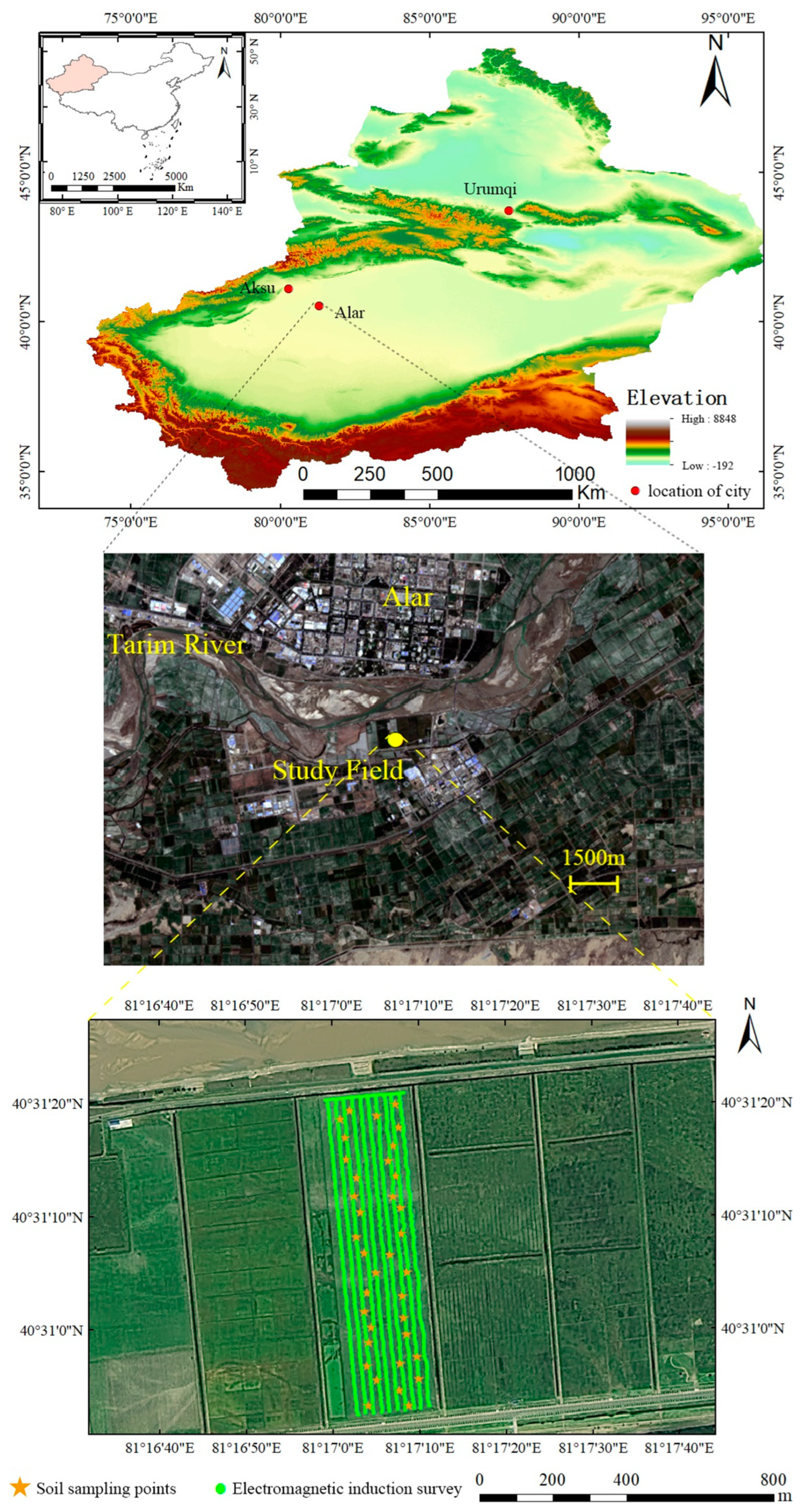
The study area is located in the National Agricultural Science and Technology Park in Alar, Xinjiang, China, as shown in Figure 1, with its central coordinates of 81°17′8″E and 40°31′8″N. The study area is approximately 900 m long from north to south and 200 m long from east to west, the study area is 18 ha, with a shortest linear distance from the Tarim river to the north of 110 m. The irrigation water source is drawn from the Aksu and Tarim rivers, the main cotton is Xinluzhong 78, the planting method is mulching [32]. The irrigation mode is drip irrigation during the cotton reproductive period. The spring and winter irrigation is diffuse irrigation, and the water table is buried at a depth of 1.2~1.5 m. The highest temperature in the study area in a year occurred in July (37.8 °C) and the lowest temperature was in July. The maximum and minimum temperatures were 37.8 °C and −8.6 °C in July and January (−8.6 °C), respectively, and the evapotranspiration ratio was about 40:1. The average sunshine duration between April and October was about 9.5 h. The annual temperature was above 10 °C and the annual total temperature reached 4113 °C. Cotton was irrigated six times during the reproductive period, with one winter irrigation and five drip irrigations (22 June, 9 July, 25 July, 13 August and 25 August). Among them, the first drip irrigation was carried out on 22 June at 450 m3/ha, and the remaining four times were carried out on 9 July, 25 July, 13 August and 25 August at 600 m3/ha, respectively, and winter irrigation was executed on November 20 at 3, 300 m3/ha.
2.2. EM38-MK2 Measurement
The EM38-MK2 consists of a transmitting coil (Tx) and two receiving coils (Rx) with a length of 1 m and a fixed operating frequency (14.6 KHz). By passing AC current through the transmitting coil and generating a primary magnetic field in the soil that gradually weakens with increasing soil depth, the magnetic field strength changes dynamically with time, causing an induced current to form in the soil, and the current induces a secondary magnetic field. The receiving coil receives both the primary magnetic field strength and the secondary magnetic field strength, and the signal receiving end can receive both the primary and secondary magnetic field signals. In automatic mode, the instrument can collect apparent conductivity data in only one mode, i.e., horizontal mode (horizontal dipole moment) or vertical mode (vertical dipole moment). In manual mode, the instrument can collect soil apparent conductivity data for both horizontal and vertical modes. The distance between the transmitter coil and the two receiver coils is 0.5 m and 1 m, respectively, and the measurement depths are 0.375 m and 0.75 m in the horizontal mode and 0.75 m and 1.5 m in the vertical mode. The new EM38-MK2 model also adopts new technology to automatically perform temperature compensation, correct circuit faults, and eliminate data drift caused by the temperature variations. the instrument has a built-in GPS.
2.3. Irrigation and Rainfall Events
Soil samples and apparent conductivity data were collected three times in June, July, and August. The key reasons for choosing these three periods for the study were, first, that all three periods were times of high-water demand and high irrigation in oasis cotton fields. Second, that the actual irrigation time in the study area was mostly concentrated in June, July, and August during the cotton growth period. In addition, considering that the study area had not been irrigated once from the end of winter irrigation last year to the beginning of June, and that the first drip irrigation was carried out on 22 June, the collection time was 20 June. 450 m3/h2 was irrigated by drip irrigation on 22 June. In addition, the rainfall in the sample area was difficult to influence the actual irrigation amount because the planting method was mulching, and the water obtained from rainfall was difficult to penetrate into the soil.
2.4. ECa Data Collection
The experiments were conducted using a geodetic conductivity meter EM38-MK2 for apparent electrical conductivity (ECa, mS m−1) measurements, which was divided into 10 measurement rows with a spacing of 20 m according to the width of the test area. Data were collected on 20 June (before the first drip irrigation), 7 July (before the second drip irrigation), and 15 August (before the third drip irrigation), 2018, and a total of three times for apparent conductivity data, using EM38-MK2 vertical and horizontal measurement modes once each, and a total of 10 measurement rows from south to north, with the instrument set to automatic recording mode and a frequency of one set of data collection per second The distribution of EM38-MK2 measurement points and soil sampling profile points is shown in Figure 1.
2.5. Soil Samples Collection
A total of three collections of apparent conductivity and soil-profile samples were conducted on 20 June, 7 July, and 15 August, 2018, and after the EM38 automatic mode collection was completed, the range of apparent conductivity in the study area was determined based on the size of the measured apparent conductivity dataset with the maximum and minimum values as the upper and lower limits, respectively, and the obtained apparent conductivity dataset was divided into 36 gradients, and in turn, according to the divided The manual mode apparent conductivity data and soil-profile samples were collected simultaneously according to the divided apparent conductivity gradient; the apparent conductivity data of the sampling points were recorded, and 36 soil-profile sample points were collected each time (Figure 1). Soil profiles were sampled in layers from 0 to 20, 20 to 40, 40 to 60, 60 to 80, and 80 to 100 cm, and the collected soil-profile samples were placed in self-sealing bags and numbered, and brought back to the laboratory for timely soil moisture determination using the mass drying method. In 2018 a total of three surveys were conducted in June, July and August, each with 36 profiles, and a total of 180 different soil-profile samples were collected in a single survey, for a total of 540 soil-profile samples throughout the year.
To calculate the irrigation volume needed to obtain soil capacity and field water-holding data, soil profile excavation and ring knife soil samples were collected on 27 October 2018, after soil auger-sampling was completed. The sample locations were selected by the EM38-MK2 automatic mode to obtain high and low values of apparent conductivity points to determine the range of modeling independent variables, and 30 of them were selected according to the apparent conductivity data close to a certain gradient, and each point was first collected for apparent conductivity data. Then, the soil profile was excavated to a depth of 70 cm, and one ring knife soil sample was taken at every 20 cm depth to collect a depth of 60 cm, for a total of 90. A total of 90 ring-knife soil samples were collected to determine soil bulk and field water-holding capacity data.
2.6. Establishing Model between Soil Water and ECa
The measured water contents of 36 sets of soil-profile samples collected in each cycle were sorted according to their numerical values, and the modeling and validation samples were drawn in a ratio of 2:1, i.e., two of every three adjacent samples were randomly selected as modeling data with the remaining one as validation data, and these were finally divided into 24 sets of modeling data and 12 sets of validation data. With the soil apparent conductivity data measured by the EM38-MK2 vertical model as the independent variable and the measured soil-moisture value as the dependent variable, the decomposition model between the soil-moisture content and soil apparent conductivity was constructed by the multiple linear regression method, and the modeling ideas were divided into two kinds of local modeling and global modeling, with local modeling as a single-period model and monthly modeling in June, July and August, respectively, and a total of three models using local modeling as a single-period model. June, July and August were modeled separately, and a total of three models were built. The global model is a multi-period mixed model, i.e., a unified model was built for all samples of the three periods. Determination coefficient (R2), root mean square error (RMSE), relative percent deviation (RPD) and mean relative error (MRE) were used to evaluate the stability and prediction accuracy of the model. Among them, the coefficient of determination reflected the degree of fit between the predicted and measured values; the root mean square error measured the deviation between the observed and true values; the mean relative error reflected the actual error of the predicted values; and the relative analytical error was an indicator of the predictive ability of the model, which was the ratio of the sample standard deviation to the root mean square error [34].
where is the predicted value, and is the measured value. where is the average value. n was the sample number. SD is the standard deviation.
2.7. Calculation Method of Drip Irrigation Cotton Field Soil Irrigation
The irrigation data in this study were the difference between the field water-holding capacity and the actual soil volumetric water content, where the field water-holding capacity was a stable property of the soil with little temporal variability, so it was considered as a stable value. The value was considered as the average of the measured field water-holding capacity. The actual soil volumetric water content was the product of the mass water content and the soil bulk weight, and the mass water content was obtained from the inversion of the apparent conductivity of each soil layer in each period. The mass water content was calculated from the apparent conductivity inversion model for each period. Soil capacity was also considered as a stable property of the soil, and was considered as the average of the measured soil capacity data to facilitate the irrigation volume calculation. taking into account only the maximum irrigation volume in the field as the field water-holding capacity. The formula for calculating the irrigation volume was:
where θi is the irrigation volume in m3 ha−1, S is the area per hectare in m2, h is the soil depth in m, ρ is the soil bulk weight in g cm−3, and θm is the mass water content of the soil to be irrigated in g kg−1.
The irrigation amount for different depth profiles of soil was calculated differently. The irrigation amount for 0~40 cm was the sum of 0~20 cm and 20~40 cm, the irrigation amount for 0~60 cm was the sum of 0~20 cm, 20~40 cm, and 40~60 cm, and so on.
3. Results
3.1. Statistics Assessment of Soil Moisture Data
Table 1 shows an overview of the measured water content data for each soil profile in three periods. Given the proximity of the test area to the Tarim River and the burial depth of groundwater mostly located at 1.2~1.5 m, the maximum, minimum and average values of soil-water content increased with the increase of soil depth in the same period. In terms of spatial variability of soil moisture in the test area, the coefficient of variation of soil-moisture content in Table 1 decreased as soil depth increased in the same period. The spatial variability of soil moisture in the surface layer (0–20 cm) was large, and the spatial variability of soil moisture in the bottom layer 80–100 cm was not obvious. From multiple periods in the same soil layer, the spatial variability of soil-moisture content in the surface layer 0–20 cm decreased gradually as the irrigation frequency increased. The variability coefficients of soil-water content in the bottom 60~80 cm and 80~100 cm had less variability in the three periods. After a preliminary analysis, from June to August, the environmental temperature kept rising and, theoretically, the rate of soil-water dissipation increased, but after several rounds of irrigation and the elevation of groundwater levels due to the flood season of Tarim River, the water content of the bottom layer, especially the 60~80 cm and 80~100 cm soil layers, increased and maintained a small spatial variability both in space and time.
3.2. Comparison of Accuracy of Soil Moisture Inversion Models
Multiple linear regression relationships between soil-moisture content and ECa at five different depths and three different times are given in Table 2. 24 profiles (modeling dataset) and were established between ECa values and validated using the remaining 18 profiles (validation dataset) at two depths measured by EM38-MK2; the R2 obtained ranged from 0.61~0.89.
Table 3 shows the fit between the predicted soil-moisture content and the soil-moisture content of the reserved validation set for each soil layer in the three periods. The p-values obtained by F-test of all models were less than 0.01. The R2 of the apparent conductivity inversion soil moisture model for the surface layer 0–20 cm in June, July and August were all higher than 0.80, and the RPD values were around 2.50, indicating that the predicted soil-moisture content of the surface layer (0–20 cm) in these three periods fit well with the measured values. The R2 and RPD values of the inversion model of the apparent conductivity of 80–100 cm in June and August were the lowest among the five soil layers in the same period, indicating that the prediction error of the inversion model of the apparent conductivity of 80–100 cm in June and August was higher than that of the other soil layers. After preliminary analysis, considering the leaching effect of winter irrigation on the salts in the soil, the salts were leached to below 1 m. However, the cotton field did not have any irrigation activity after the previous year’s winter irrigation until the first irrigation in 2018, and with the gradual recovery of ground temperature in spring, some of the soluble soil salts also formed a re-salt zone with the rising movement of soil moisture, which in turn affected the apparent conductivity values in the re-salt zone, leading to the stability of the model and its prediction. The stability of the model and its prediction ability decreased.
From the end of winter irrigation in the previous year to June, along with the gradual increase of ambient temperature in the study area, the apparent conductivity inversion model R2 of the soil layer deeper than 20 cm showed a decrease trend with increasing soil depth, and so did RPD. In addition to the influence cause by soil salinity, the degree of spatial variability of soil moisture itself can further cause error variation. As shown in Table 1, the coefficient of variation of soil-moisture content in different soil layers in the same period decreased as the soil depth increased, from which it was inferred that the spatial variability of soil-moisture content in the bottom layer (80–100 cm) in June was smaller, and the degree of spatial variability of soil moisture was relatively low. The prediction error of the inverse model prediction increased, and its predictive ability was not as good as that of other soil layers in the same period.
Comparing the results in June with July, first, in terms of influence caused by crop growth metabolic activities in July, the water requirement of cotton reached its highest at the boll stage and the root system was most active. Second, in terms of soil moisture changes, after the first irrigation in the cotton field, the root layer under the film, especially the surface soil moisture, was fully replenished. Finally, in terms of changes in the apparent conductivity inversion model of the same soil layer for two periods, the R2, RMSE and RPD values of the apparent conductivity inversion model at 0–20 cm changed less while the MRE decreased. Additionally, in July, the R2 and RPD values at 20–40 cm were the lowest and MRE was the highest among the five soil layers, so the stability and accuracy of the inversion model of this layer were relatively low.
The average monthly temperature in August was at the highest temperature of the year, and the metabolic activities of cotton slowed down compared with July, and the water demand gradually decreased. Although the cotton field was irrigated several times, the water content of the surface soil still decreased compared with that in July. The five soil apparent conductivity inversion models for the same period did not have regularity under the interactions of multiple factors dominated by temperature. Compared with the same soil layer apparent conductivity inversion model in July, both R2 and RPD values obtained by apparent conductivity model at the 20–40 cm soil layer increased in August, so the stability and predictive ability of the model were improved.
From the evaluation indicators in Table 3, the linear inversion model soil moisture was possible in most cases. For agricultural fields in arid regions, the water–salt ratio in the soil not only directly affects the soil apparent conductivity values, but also is a crucial factor for high crop yield. In the following, the influence of two aspects on the predictive ability of the model, the degree of spatial variability in different soil layers and soil salinity, will be discussed. First, in terms of the spatial variability of soil moisture in different soil layers, as shown in Table 1 and Table 3, when the degree of spatial variability of soil moisture is large (e.g., 0–20 cm soil layer in the same period), the R2 value of the multivariate linear model was high, and the RPD value was also at a high level, indicating that the predictive ability of the model was high. In contrast, when the spatial variability of soil moisture was small (e.g., 80–100 cm depth in the same period), the predictive ability of the multivariate linear model was lower. This relationship was not sufficient to fully account for the higher spatial variability of soil moisture, because the soil texture in the study area is homogeneous and the mulching technique was used, which aimed to increase the temperature and retain moisture and to slow down the natural loss of soil moisture and soil temperature as much as possible. Therefore, whether the degree of spatial variability of soil moisture was more favorable for model fitting and prediction for farmland with heterogeneous soil texture needed further study.
Finally, in terms of soil salinity, soil salinity was bound to affect the inversion of apparent conductivity of soil moisture to some extent. In this study (Table 4), the mean value of apparent conductivity at 0.375 m in June (35.21 mS m−1) was lower than the mean value of apparent conductivity at 0.75 m (54.30 mS m−1), based on the positive correlation between apparent conductivity and soil-salinity content in agricultural soils, as well as previous related studies on the spatial and temporal variability of soil salinity [35], indicating that the soil-salt content located in the rhizosphere, especially in the 20–40 cm soil layer, was lower than that in the non-rhizosphere (below 60 cm) in June. the predictive ability of the 20–40 cm apparent conductivity model was better than that of the non-root layer apparent conductivity model. However, the mean values of apparent conductivity in July were 117.03 mS m−1 and 112.60 mS m−1 at 0.375 m and 0.75 m, respectively, and 78.75 mS m−1 at 1.5 m, indicating that the difference in soil salinity content between 0.375 m and 0.75 m during this period was not significant. While the soil salinity content at 1.5 m was very low, indicating that its soil salinity was The R2 of the apparent conductivity model at 20–40 cm in July was 0.60, and the accuracy of the model was reduced compared with that in June. Therefore, although salinity had a certain influence on soil moisture inversion in a few soil layers, and this influence effect reduced the degree of fit between the predicted and measured values of the model, the model still had considerable predictive ability and could be applied practically.
3.3. Comparison between Multi-Period and Single-Period Model
To investigate whether EM38-MK2 could be directly applied to multi-period applications, the full-period model and the single-period model were developed in this study (Table 5), and the comparison of evaluation indexes of each model is shown in Table 6. Comparing the two modeling ideas for the same soil layer, it can be seen that the R2 and RPD values of the single-period model for each soil layer water content model were higher than the full-period model, and the MRE value was lower than the full-period model. After preliminary analysis, on the one hand, agricultural soils are non-homogeneous, and soil salinity is constantly moving up and down in the vertical direction by irrigation and evapotranspiration. On the other hand, the influence of higher ambient temperature easily triggers evapotranspiration water consumption, which can affect the variability of soil-water content in the horizontal direction. The highest RPD of the full period model was 1.38 and the lowest RPD of the single period model was 1.33, indicating that the multi-period model of apparent conductivity inversion of soil-water content has good predictive ability and high stability. The lowest coefficient of determination was found in the full-period model at 40–60 cm, which is presumed to be the result of soil water uptake by directional growth of a few main crop roots at this depth, coupled with changes in ambient temperature. Since the predictive ability of the full-period model was not as good as that of the single-period model, this suggests that the parameter of multiple-period model cannot be applied to a simple linear model at a specific period, but a separate set of linear model parameters should be used for each period.
3.4. Distribution of Irrigation Amount
Table 7 shows the statistical results of soil bulk density and field capacity of the soil samples. The results show that the coefficient variation of both at the field scale in the study area was not higher than 10%, and the degree of variation was small. Therefore, the average values of 1.48 g cm3 and 25.44% for soil-bulk density and soil-field capacity can be used as the desired target values for both in field-scale irrigation calculations. This value can be used as soil capacity and field water-holding capacity in the calculation of irrigation volume at the field scale.
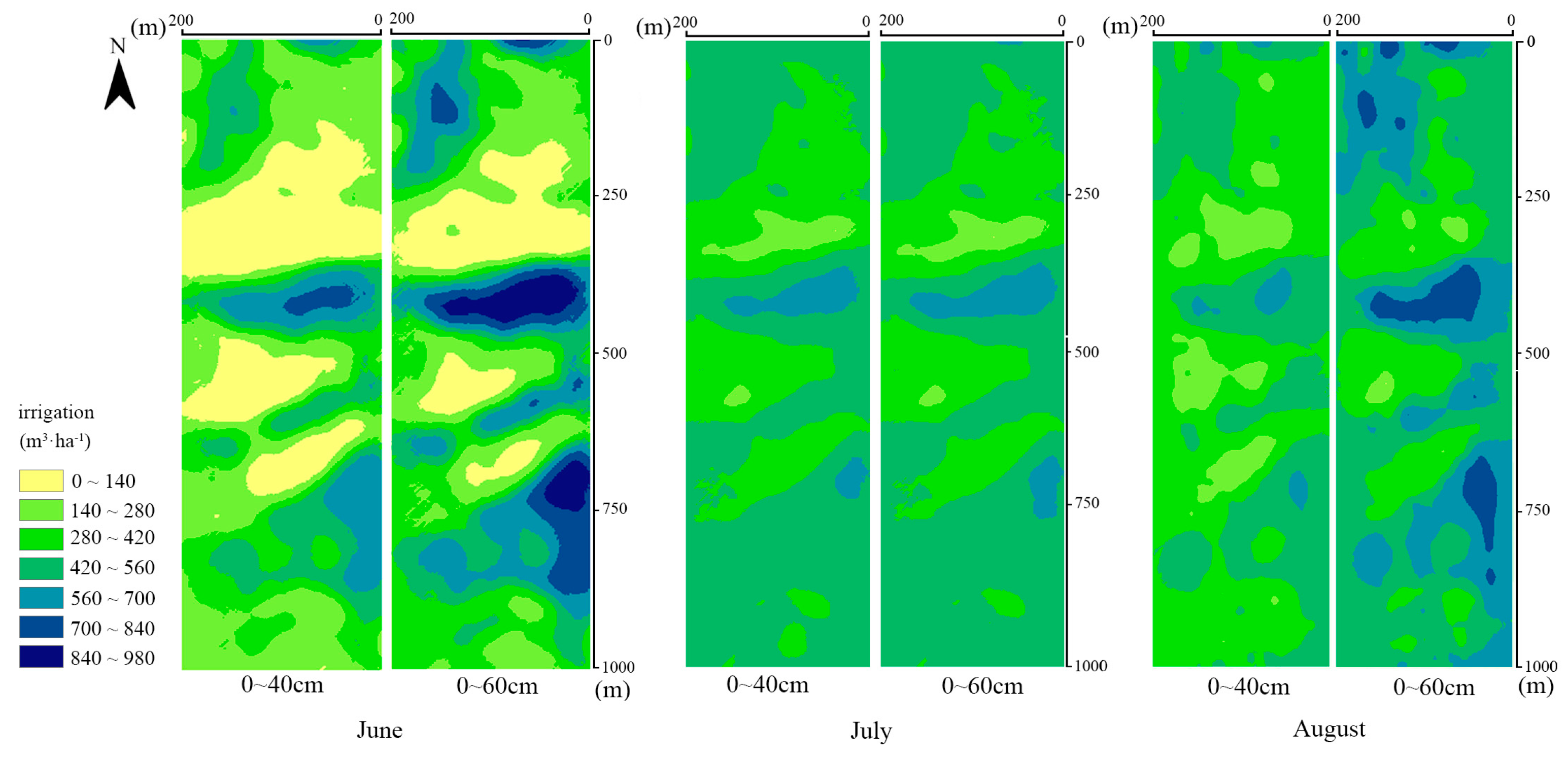
Kriging, also known as spatial local interpolation, is a method for te unbiased optimal estimation of regionalized variables in a finite area based on variance function theory and structural analysis and is one of the main elements of geo-statistics. In this study, the soil apparent conductivity data obtained from EM38 automatic model was brought into the soil-moisture estimation model to calculate the soil-water content in the study area, and the irrigation amount in the study area was calculated by Equation (5). The ordinary kriged land statistical in inversion interpolation method was selected for irrigation volume distribution mapping. The interpolated irrigation volume distribution map was first rasterized, and then the rasterized data were reclassified according to the legend in Figure 2 as the grading standard, and the number of rasterized cells at each level was counted. The theoretical irrigation volume was calculated by taking the median value at each level. Figure 2 shows the distribution of irrigation amount in June, July, and August, respectively.
First, from the overall spatial distribution, the northern part of the study area is adjacent to the Tarim River, and most of the area has less irrigation water than the southern part. The high irrigation-volume amount in the northern part of the study area is mainly located in a small part of the northeast corner of the study area, and a small part of about 500 m from north to south. The high irrigation-volume amount in the northern part of the study area is mainly due to the high apparent soil conductivity. By combining previous studies on apparent conductivity and soil salinity [35,36], it was shown that in areas with a high apparent conductivity, soil-salinity content is also high [37]. So, the soil salinity content in the high irrigation volume area is slightly higher than other areas in the study area. In addition, during the field survey, it was found that a small portion of the bare soil in the high irrigation area appeared to have a white color at the topsoil, and the cotton crop planted was short with a very low seedling emergence rate. It can be judged that the soil-salt concentration in this area exceeded the salt-tolerance threshold of the crop, and thus affected the growth of the crops. The accumulation of salt crusts caused the “whitening phenomenon” in the topsoil. A small part of the northeast corner of the study area with high irrigation is mainly affected by the flood the Tarim River in dry periods. The area of high irrigation in the southern of the study area is located in the eastern of the study area from north to south for 750 m. The field survey found that this high irrigation area is also affected by high apparent soil conductivity. Although the soil salinization is similar to the high irrigation area in the northern of the study area for 500 m, it exists only at topsoil (10 cm). Unlike the area with high irrigation in the northern for 500 m, the eastern part for 750 m rarely has seedling emergence, so it is assumed that the soil with high apparent conductivity in the topsoil (10 cm) does not threatens the growth of crops in this area. The height and emergence rate of cotton crops are consistent with the surrounding area, and the top does not appear to have the “whitening phenomenon”.
Second, in terms of the temporal variation, the distribution of irrigation amount at depths of 0–40 cm and 0–60 cm in June tended to be consistent with the overall color distribution at both depths in June. The highest irrigation volume was greater than 700 m3 ha−1 at the above-mentioned highly irrigated areas. The average monthly ambient temperature in July increased compared to June, and the rate of water loss from the topsoil located in the non-film covered areas increased compared to June, as can be seen in Figure 2. The yellow area with irrigation volume lower than 140 m3 ha−1 disappeared in July, both the minimum irrigation volume at the depths of 0–40 cm and 0–60 cm increased compared to June. The gray area with irrigation amount of 420–560 m3 ha−1 accounted for the largest percentage, indicating that the irrigation amount increased significantly in July compared to June. From July to August, although the water demand of cotton roots gradually slowed down, the average monthly temperature was still increasing, as shown by a significant decrease in the percentage of gray area with irrigation volume of 420–560 m3 ha−1 but still concentrated in the northeast corner, 500 m area from north to south and 750 m east area. Comparing the locations of the high irrigation areas in June, we can see that the locations are basically the same of the above three areas in August. Therefore, in the actual irrigation process, we should specify the appropriate irrigation strategy to avoid the reduction of crop yield in cotton fields due to insufficient irrigation.
With the research on soil water management plans for agricultural fields in recent years [38], the monitoring and management of soil water dynamics has received much attention. As a typical arid farmland in South Xinjiang, the soil moisture in this study area is strongly heterogeneous in space due to the arid climate and high evapotranspiration ratio. The soil-moisture distribution is described as “dry at the top and wet at the bottom layer”, which is not conducive to farmers’ accurate estimation of soil-moisture content of farmland and causes excessive irrigation. On the other hand, at present, the irrigation scheme mostly adopts a same irrigation strategy to the total farmland. This irrigation method not only causes waste of soil water in the local area with low irrigation volume, but also leads to insufficient irrigation water in the local area with high irrigation volume, which leads to yield reduction.
Compared with the actual irrigation volume, the irrigation amount obtained by inversion model in this study saved 163.07, 161.32, and 208.46 m3 ha−1 in June, July, and August at the depth of 0–40 cm, respectively; saved 58.43, 156.24, and 91.79 m3 ha−1 in June, July, and August at the depth of 0–60 cm, respectively. The 0–60 cm saved 58.43, 156.24 and 91.79 m3 ha−1 of irrigation in June, July, and August, respectively. Thus, only considering soil moisture, the method used in this study can reduce irrigation amount by at least 160 m3 ha−1 for crops with shallow root depths and reduce about 30% and 15% in July and August for crops or fruit trees at deep root depths, but less in June. By contrast to the results of previous studies, this study aimed to reduce the waste of soil moisture by using a fine-grained regional irrigation amount. The field-scale inversion of soil moisture is more effective in keeping an eye on soil-moisture conditions in highly irrigated areas, while facilitating rapid information on soil-moisture distribution at the farm scale. However, only the soil-moisture condition was considered in this study, and the content of soil moisture requiring salt leaching in highly irrigated areas was missing. Therefore, future studies will subsequently concentrate on the assessment of the effect of soil-salt concentrations on the uptake of soil moisture by crops in multiple water-demand periods, so that the irrigation amount can effectively alleviate the physiological drought of crops, and be applied to the leaching of soil salts to meet the requirements for more demand under-membrane drip irrigation systems in arid areas of Xinjiang.
4. Conclusions
In this study, an inversion of field-scale soil-moisture data was performed using the apparent soil conductivity of cotton fields obtained by EM38-MK2. The results from the inversion model showed that the linear-inversion approach of soil moisture using soil apparent conductivity data was feasible. Moreover, the ability of the inversion model to be directly applied to multiple periods was also investigated, and the results showed that the predictive ability of the full-period model was not as good as that of the single-period model, indicating that the inversion model of soil-moisture content for multiple periods cannot be directly applied to a simple model for a specific period, and a separate set of models should be used for each period separately, which can improve the accuracy of prediction of soil moisture. In this study, soil-irrigation volume distribution was also mapped by simple kriging interpolation method combined with soil-moisture capacity and field water-holding capacity data, taking into account only soil-moisture conditions. By comparing these with the actual irrigation volume, the predicted field-irrigation volume for all three periods was less than the actual irrigation volume, refining the regional irrigation volume and reducing the waste of soil moisture. Therefore, the geodetic conductivity meter used in this study can achieve the purpose of guiding irrigation amounts to a certain extent by the inversion of soil moisture, soil-moisture capacity and field water-holding capacity data under the premise of considering soil moisture only.
Author Contributions
All authors contributed in a substantial way to the manuscript. J.H.: conceived and designed the research themes analyzed the data. C.F.: contribution to data analysis. N.W.: contributed to the revision and translation. M.W.: contributed to revision and translation. J.W.: contributed to the revision. J.P.: conceived and designed the research themes analyzed the data. All authors have read and agreed to the published version of the manuscript.
Funding
This research was supported by grants from the Tarim University President’s Fund (Grant Nos. TDZKCX202205, TDZKSS202227, TDZKSS202350), the Bingtuan Science and Technology Program (Grant No. 2020CB032), the National Key Research and Development Program of China (Grant No. 2018YFE0107000).
Data Availability Statement
Not applicable.
Conflicts of Interest
The authors declare no conflict of interest.
References
- Fereres, E.; Soriano, M.A. Deficit Irrigation for Reducing Agricultural Water Use. J. Exp. Bot. 2007, 58, 147–159. [Google Scholar] [CrossRef] [Green Version]
- Misra, R.K.; Padhi, J. Assessing Field-Scale Soil Water Distribution with Electromagnetic Induction Method. J. Hydrol. 2014, 516, 200–209. [Google Scholar] [CrossRef]
- Wijewardana, Y.G.N.S.; Galagedara, L.W. Estimation of Spatio-Temporal Variability of Soil Water Content in Agricultural Fields with Ground Penetrating Radar. J. Hydrol. 2010, 391, 24–33. [Google Scholar] [CrossRef]
- Li, P.; He, S.; He, X.; Health, R.T.-E. Seasonal Hydrochemical Characterization and Groundwater Quality Delineation Based on Matter Element Extension Analysis in a Paper Wastewater Irrigation Area; Springer: Berlin/Heidelberg, Germany, 2018; Volume 10, pp. 241–258. [Google Scholar] [CrossRef]
- Foster, S.; Chilton, J.; Nijsten, G.J.; Richts, A. Groundwater-a Global Focus on the “Local Resource”. Curr. Opin. Environ. Sustain. 2013, 5, 685–695. [Google Scholar] [CrossRef]
- Dalton, F.N. Development of Time-Domain Reflectometry for Measuring Soil Water Content and Bulk Soil Electrical Conductivity. In Advances in Measurement of Soil Physical Properties: Bringing Theory into Practice; Wiley: New York, NY, USA, 2012; pp. 143–167. ISBN 9780891189251. [Google Scholar]
- Triantafilis, J.; Kerridge, B.; Journal, S.B.-A. Digital Soil-class Mapping from Proximal and Remotely Sensed Data at the Field Level. Agron. J. 2009, 101, 841–853. [Google Scholar] [CrossRef]
- Altdorff, D.; Sadatcharam, K.; Unc, A.; Krishnapillai, M.; Galagedara, L. Comparison of Multi-Frequency and Multi-Coil Electromagnetic Induction (Emi) for Mapping Properties in Shallow Podsolic Soils. Sensors 2020, 20, 2330. [Google Scholar] [CrossRef] [PubMed] [Green Version]
- Visconti, F.; Science, J.D.P.-E.J. of S. A Semi-empirical Model to Predict the EM38 Electromagnetic Induction Measurements of Soils from Basic Ground Properties. Eur. J. Soil Sci. 2021, 72, 720–738. [Google Scholar] [CrossRef]
- Xie, W.; Yang, J.; Yao, R.; Wang, X. Article Spatial and Temporal Variability of Soil Salinity in the Yangtze River Estuary Using Electromagnetic Induction. Remote. Sens. 2021, 13, 1875. [Google Scholar] [CrossRef]
- Corwin, D.; Analysis, J.R. soil science and plant. Establishing Soil Electrical Conductivity-Depth Relations from Electromagnetic Induction Measurements. Commun. Soil Sci. Plant Anal. 1990, 21, 861–901. [Google Scholar] [CrossRef]
- Zare, E.; Arshad, M.; Zhao, D.; Nachimuthu, G.; Triantafilis, J. Two-Dimensional Time-Lapse Imaging of Soil Wetting and Drying Cycle Using EM38 Data across a Flood Irrigation Cotton Field. Agric. Water Manag. 2020, 241, 106383. [Google Scholar] [CrossRef]
- Huth, N.; Research, P.P.-S. An Electromagnetic Induction Method for Monitoring Variation in Soil Moisture in Agroforestry Systems. Soil Res. 2007, 45, 63–72. [Google Scholar] [CrossRef]
- Dunn, B.W.; Beecher, H.G. Using Electro-Magnetic Induction Technology to Identify Sampling Sites for Soil Acidity Assessment and to Determine Spatial Variability of Soil Acidity in Rice Fields. Aust. J. Exp. Agric. 2007, 47, 208–214. [Google Scholar] [CrossRef]
- Wienhold, B.J. Apparent Electrical Conductivity for Delineating Spatial Variability in Soil Properties. In Handbook of Agricultural Geophysics; CRC Press, Taylor and Francis Group: Boca Raton, FL, USA; pp. 211–215. ISBN 9781420019353.
- Van Meirvenne, M.; Islam, M.M.; De Smedt, P.; Meerschman, E.; Van De Vijver, E.; Saey, T. Key Variables for the Identification of Soil Management Classes in the Aeolian Landscapes of North-West Europe. Geoderma 2013, 199, 99–105. [Google Scholar] [CrossRef]
- Jung, W.K.; Kitchen, N.R.; Sudduth, K.A.; Kremer, R.J.; Motavalli, P.P. Relationship of Apparent Soil Electrical Conductivity to Claypan Soil Properties. Soil Sci. Soc. Am. J. 2005, 69, 883–892. [Google Scholar] [CrossRef] [Green Version]
- White, M.L.; Shaw, J.N.; Raper, R.L.; Rodekohr, D.; Wood, W. A Multivariate Approach for High-Resolution Soil Survey Development. Soil Sci. 2012, 177, 345–354. [Google Scholar] [CrossRef] [Green Version]
- Cockx, L.; Van Meirvenne, M.; Vitharana, U.W.A.; Verbeke, L.P.C.; Simpson, D.; Saey, T.; Van Coillie, F.M.B. Extracting Topsoil Information from EM38DD Sensor Data Using a Neural Network Approach. Soil Sci. Soc. Am. J. 2009, 73, 2051–2058. [Google Scholar] [CrossRef]
- Vitharana, U.W.A.; Van Meirvenne, M.; Simpson, D.; Cockx, L.; De Baerdemaeker, J. Key Soil and Topographic Properties to Delineate Potential Management Classes for Precision Agriculture in the European Loess Area. Geoderma 2008, 143, 206–215. [Google Scholar] [CrossRef]
- Jaynes, D.B. Mapping the Areal Distribution of Soil Parameters with Geophysical Techniques. In Applications of GIS to the Modeling of Non-Point Source Pollutants in the Vadose Zone; Wiley: New York, NY, USA, 2015; pp. 205–216. ISBN 9780891189435. [Google Scholar]
- Johnson, C.K.; Doran, J.W.; Duke, H.R.; Wienhold, B.J.; Eskridge, K.M.; Shanahan, J.F. Field-Scale Electrical Conductivity Mapping for Delineating Soil Condition. Soil Sci. Soc. Am. J. 2001, 65, 1829–1837. [Google Scholar] [CrossRef] [Green Version]
- Martinez, G.; Vanderlinden, K.; Ordóñez, R.; Muriel, J.L. Can Apparent Electrical Conductivity Improve the Spatial Characterization of Soil Organic Carbon? Vadose Zone J. 2009, 8, 586–593. [Google Scholar] [CrossRef]
- Doolittle, J.A.; Brevik, E.C. The use of electromagnetic induction techniques in soils studies. Geoderma 2014, 223, 33–45. [Google Scholar] [CrossRef] [Green Version]
- Friedman, S.P. Soil Properties Influencing Apparent Electrical Conductivity: A Review. Comput. Electron. Agric. 2005, 46, 45–70. [Google Scholar] [CrossRef]
- Heilig, J.; Kempenich, J.; Doolittle, J.; Brevik, E.C.; Ulmer, M. Evaluation of Electromagnetic Induction to Characterize and Map Sodium-Affected Soils in the Northern Great Plains. Soil Horizons 2011, 52, 77. [Google Scholar] [CrossRef]
- Kachanoski, R.G.; Gregorich, E.G.; Van Wesenbeeck, I.J. Estimating Spatial Variations of Soil Water Content Using Noncontacting Electromagnetic Inductive Methods. Can. J. Soil Sci. 1988, 68, 715–722. [Google Scholar] [CrossRef]
- Calamita, G.; Perrone, A.; Brocca, L.; Onorati, B.; Manfreda, S. Field Test of a Multi-Frequency Electromagnetic Induction Sensor for Soil Moisture Monitoring in Southern Italy Test Sites. J. Hydrol. 2015, 529, 316–329. [Google Scholar] [CrossRef]
- Hanson, B.R.; Kaita, K. Response of Electromagnetic Conductivity Meter to Soil Salinity and Soil-Water Content. J. Irrig. Drain. Eng. 1997, 123, 141–143. [Google Scholar] [CrossRef]
- Huang, J.; Scudiero, E.; Clary, W.; Corwin, D.L.; Triantafilis, J. Time-Lapse Monitoring of Soil Water Content Using Electromagnetic Conductivity Imaging. Soil Use Manag. 2017, 33, 191–204. [Google Scholar] [CrossRef]
- Huang, J.; Purushothaman, R.; McBratney, A.; Bramley, H. Soil Water Extraction Monitored per Plot across a Field Experiment Using Repeated Electromagnetic Induction Surveys. Soil Syst. 2018, 2, 11. [Google Scholar] [CrossRef] [Green Version]
- Hossain, M.B.; Lamb, D.W.; Lockwood, P.V.; Frazier, P. EM38 for Volumetric Soil Water Content Estimation in the Root-Zone of Deep Vertosol Soils. Comput. Electron. Agric. 2010, 74, 100–109. [Google Scholar] [CrossRef]
- Li, X.; Shao, M.A.; Zhao, C.; Liu, T.; Jia, X.; Ma, C. Regional spatial variability of root-zone soil moisture in arid regions and the driving factors—A case study of Xinjiang, China. Can. J. Soil Sci. 2019, 99, 277–291. [Google Scholar] [CrossRef]
- Kayacan, E.; Kayacan, E.; Ramon, H.; Saeys, W. Towards Agrobots: Identification of the Yaw Dynamics and Trajectory Tracking of an Autonomous Tractor. Comput. Electron. Agric. 2015, 115, 78–87. [Google Scholar] [CrossRef] [Green Version]
- Khongnawang, T.; Zare, E.; Srihabun, P.; Khunthong, I.; Triantafilis, J. Digital soil mapping of soil salinity using EM38 and quasi-3d modelling software (EM4Soil). Soil Use Manag. 2022, 38, 277–291. [Google Scholar] [CrossRef]
- Zarai, B.; Walter, C.; Michot, D.; Montoroi, J.P.; Hachicha, M. Integrating multiple electromagnetic data to map spatiotemporal variability of soil salinity in Kairouan region, Central Tunisia. J. Arid. Land 2022, 14, 186–202. [Google Scholar] [CrossRef]
- Li, H.; Liu, X.; Hu, B.; Biswas, A.; Jiang, Q.; Liu, W.; Wang, N.; Peng, J. Field-Scale Characterization of Spatio-Temporal Variability of Soil Salinity in Three Dimensions. Remote Sens. 2020, 12, 4043. [Google Scholar] [CrossRef]
- Hedley, C.B.; Yule, I.J. A Method for Spatial Prediction of Daily Soil Water Status for Precise Irrigation Scheduling. Agric. Water Manag. 2009, 96, 1737–1745. [Google Scholar] [CrossRef]
Figure 1.
Location of study area, sampling points of electromagnetic induction survey. and soil sampling.
Figure 1.
Location of study area, sampling points of electromagnetic induction survey. and soil sampling.

Figure 2.
Distribution of irrigation in June, July and August.


Table 1.
Statistics of measured soil moisture. Note: Max, Maximum; Min, Minimum; Mean, Arithmetic mean; CV, Coefficient of Variation.
Table 1.
Statistics of measured soil moisture. Note: Max, Maximum; Min, Minimum; Mean, Arithmetic mean; CV, Coefficient of Variation.
| Month | Depth (cm) | Max (%) | Min (%) | Mean (%) | CV(%) |
|---|---|---|---|---|---|
| June | 0~20 | 17.34 | 8.25 | 12.38 | 23.91 |
| 20~40 | 21.89 | 14.15 | 17.63 | 14.55 | |
| 40~60 | 25.82 | 13.91 | 21.16 | 13.43 | |
| 60~80 | 28.96 | 19.59 | 24.65 | 8.23 | |
| 80~100 | 30.37 | 20.95 | 26.39 | 8.22 | |
| July | 0~20 | 27.19 | 13.27 | 17.32 | 18.06 |
| 20~40 | 28.15 | 17.42 | 21.04 | 11.38 | |
| 40~60 | 27.83 | 15.92 | 23.44 | 15.29 | |
| 60~80 | 29.52 | 18.82 | 26.34 | 9.39 | |
| 80~100 | 32.43 | 24.36 | 27.95 | 8.40 | |
| August | 0~20 | 21.84 | 11.98 | 15.39 | 14.99 |
| 20~40 | 25.80 | 15.47 | 19.39 | 12.67 | |
| 40~60 | 27.32 | 17.30 | 23.78 | 13.32 | |
| 60~80 | 32.27 | 21.25 | 27.57 | 9.21 | |
| 80~100 | 32.50 | 23.52 | 28.27 | 6.97 |
Table 2.
Predicted relationships of soil-water content at different depths and periods.
| Month | Depth (cm) | Models | R2 |
|---|---|---|---|
| June | 20 | y = 0.009X1 + 0.090X2 + 7.032 | 0.87 |
| 40 | y = 0.045X1 + 0.027X2 + 14.529 | 0.89 | |
| 60 | y = −0.027X1 + 0.110X2 + 16.929 | 0.76 | |
| 80 | y = −0.053X1 + 0.126X2 + 20.500 | 0.67 | |
| 100 | y = −0.037X1 + 0.102X2 + 22.730 | 0.61 | |
| July | 20 | y = −0.042X1 + 0.082X2 + 13.166 | 0.87 |
| 40 | y = −0.057X1 + 0.081X2 + 18.841 | 0.62 | |
| 60 | y = 0.043X1 − 0.080X2 + 27.092 | 0.77 | |
| 80 | y = 0.037X1 − 0.063X2 + 28.947 | 0.75 | |
| 100 | y = −0.032X1 + 0.007X2 + 31.02 | 0.74 | |
| August | 20 | y = −0.054X1 − 0.005X2 + 18.27 | 0.88 |
| 40 | y = 0.033X1 − 0.067X2 + 22.116 | 0.65 | |
| 60 | y = −0.085X1 + 0.035X2 + 27.41 | 0.79 | |
| 80 | y = −0.017X1 − 0.035X2 + 30.971 | 0.71 | |
| 100 | y = 0.061X1 − 0.091X2 + 30.154 | 0.7 |
Note: X1 means ECv0.75, X2 means ECv1.5.
Table 3.
Indices of cross-validation Soil Moisture Model. Note: R2, coefficient of determination; RMSE, root mean square error; RPD, Relative percent deviation; MRE, Mean relative error.
Table 3.
Indices of cross-validation Soil Moisture Model. Note: R2, coefficient of determination; RMSE, root mean square error; RPD, Relative percent deviation; MRE, Mean relative error.
| Month | Depth (cm) | R2 | RMSE (%) | RPD | MRE (%) |
|---|---|---|---|---|---|
| June | 0–20 | 0.87 | 1.80 | 2.44 | 1.26 |
| 20–40 | 0.89 | 1.33 | 2.89 | 1.10 | |
| 40–60 | 0.73 | 1.07 | 1.70 | 2.32 | |
| 60–80 | 0.64 | 0.98 | 1.38 | 0.89 | |
| 80–100 | 0.58 | 1.39 | 1.19 | 1.08 | |
| July | 0~20 | 0.86 | 0.86 | 2.50 | 0.75 |
| 20~40 | 0.60 | 1.80 | 1.13 | 2.50 | |
| 40~60 | 0.75 | 1.87 | 1.75 | 2.30 | |
| 60~80 | 0.73 | 0.91 | 1.81 | 1.56 | |
| 80~100 | 0.71 | 1.17 | 1.36 | 1.79 | |
| August | 0–20 | 0.88 | 0.66 | 2.69 | 0.57 |
| 20–40 | 0.59 | 1.73 | 1.20 | 2.99 | |
| 40–60 | 0.51 | 1.48 | 1.01 | 2.20 | |
| 60–80 | 0.72 | 1.17 | 1.62 | 0.88 | |
| 80–100 | 0.66 | 0.79 | 1.38 | 0.69 |
Table 4.
The statistical characteristic values of geospatial electromagnetic induction measurements of apparent electrical conductivity (ECa) at different periods.
Table 4.
The statistical characteristic values of geospatial electromagnetic induction measurements of apparent electrical conductivity (ECa) at different periods.
| Date | ECa | Min (mS m−1) | Max (mS m−1) | Mean (mS m−1) |
|---|---|---|---|---|
| June | ECh0.375 | 102.422 | 3.75 | 35.21 |
| ECh0.75 | 100 | 10.547 | 54.30 | |
| ECV0.75 | 173.359 | 13.086 | 65.20 | |
| ECV1.5 | 139.102 | 20.313 | 73.18 | |
| July | ECh0.375 | 145 | 34.004 | 117.03 |
| ECh0.75 | 163.535 | 23.516 | 112.06 | |
| ECV0.75 | 120.891 | 35.898 | 86.95 | |
| ECV1.5 | 160.195 | 18.516 | 78.75 | |
| August | ECh0.375 | 141.328 | 12.3635 | 65.33 |
| ECh0.75 | 159.1605 | 6.035 | 84.22 | |
| ECV0.75 | 173.6525 | 16.641 | 82.29 | |
| ECV1.5 | 165.0975 | 17.91 | 75.21 |
Table 5.
Predicted relationships of soil-water content at different depths for the whole period.
| Method | Depth (cm) | Models | R2 |
|---|---|---|---|
| Multi-period | 0~20 | Y = 0.097X1 − 0.061X2 + 12.052 | 0.54 |
| 20~40 | Y = 0.061X1 − 0.033X2 + 17.410 | 0.51 | |
| 40~60 | Y = 0.070X1 − 0.084X2 + 23.876 | 0.33 | |
| 60~80 | Y = 0.065X1 − 0.077X2 + 26.993 | 0.60 | |
| 80~100 | Y = 0.026X1 − 0.029X2 + 27.734 | 0.40 |
Table 6.
Accuracy assessment of single period model and multi-period model. Note: R2, coefficient of determination; RMSE, root mean square error; RPD, Relative percent deviation; MRE, Mean relative error.
Table 6.
Accuracy assessment of single period model and multi-period model. Note: R2, coefficient of determination; RMSE, root mean square error; RPD, Relative percent deviation; MRE, Mean relative error.
| Method | Depth (cm) | R2 | RMSE (%) | RPD | MRE (%) |
|---|---|---|---|---|---|
| Multi-period | 0~20 | 0.52 | 1.29 | 0.96 | 0.89 |
| 20~40 | 0.47 | 2.42 | 1.01 | 1.74 | |
| 40~60 | 0.26 | 2.65 | 0.54 | 2.21 | |
| 60~80 | 0.58 | 1.57 | 1.28 | 1.5 | |
| 80~100 | 0.35 | 1.34 | 1.38 | 1.58 | |
| Single period | 0~20 | 0.89 | 1.21 | 1.79 | 0.68 |
| 20~40 | 0.64 | 1.75 | 1.36 | 1.46 | |
| 40~60 | 0.79 | 1.86 | 1.63 | 1.74 | |
| 60~80 | 0.62 | 1.57 | 1.77 | 1.34 | |
| 80~100 | 0.77 | 1.47 | 1.33 | 0.84 |
Table 7.
Statistic of soil-bulk density and field capacity. Note: Max, Maximum; Min, Minimum; Mean, mean; CV, Coefficient of Variation.
Table 7.
Statistic of soil-bulk density and field capacity. Note: Max, Maximum; Min, Minimum; Mean, mean; CV, Coefficient of Variation.
| Soil Properties | Max | Min | Mean | CV |
|---|---|---|---|---|
| Bulky density (g cm−3) | 1.63 | 1.25 | 1.48 | 5% |
| Field Capacity (%) | 34.69 | 20.31 | 25.44 | 10% |
Disclaimer/Publisher’s Note: The statements, opinions and data contained in all publications are solely those of the individual author(s) and contributor(s) and not of MDPI and/or the editor(s). MDPI and/or the editor(s) disclaim responsibility for any injury to people or property resulting from any ideas, methods, instructions or products referred to in the content. |
© 2023 by the authors. Licensee MDPI, Basel, Switzerland. This article is an open access article distributed under the terms and conditions of the Creative Commons Attribution (CC BY) license (https://creativecommons.org/licenses/by/4.0/).
Share and Cite
MDPI and ACS Style
Han, J.; Wang, M.; Wang, N.; Wang, J.; Peng, J.; Feng, C. Research on Cotton Field Irrigation Amount Calculation Based on Electromagnetic Induction Technology. Remote Sens. 2023, 15, 1975. https://doi.org/10.3390/rs15081975
AMA Style
Han J, Wang M, Wang N, Wang J, Peng J, Feng C. Research on Cotton Field Irrigation Amount Calculation Based on Electromagnetic Induction Technology. Remote Sensing. 2023; 15(8):1975. https://doi.org/10.3390/rs15081975
Chicago/Turabian StyleHan, Jianwen, Mingyue Wang, Nan Wang, Jiawen Wang, Jie Peng, and Chunhui Feng. 2023. "Research on Cotton Field Irrigation Amount Calculation Based on Electromagnetic Induction Technology" Remote Sensing 15, no. 8: 1975. https://doi.org/10.3390/rs15081975
Note that from the first issue of 2016, this journal uses article numbers instead of page numbers. See further details here.