Forecasting Precipitation from Radar Wind Profiler Mesonet and Reanalysis Using the Random Forest Algorithm

Abstract

Data-driven machine learning technology can learn and extract features, a factor which is well recognized to be powerful in the warning and prediction of severe weather. With the large-scale deployment of the radar wind profile (RWP) observational network in China, dynamical variables with higher temporal and spatial resolution in the vertical become strong supports for machine-learning-based severe convection prediction. Based on the RWP mesonet that has been deployed in Beijing, this study uses the measurements from four triangles composed of six RWP stations to determine the profiles of divergence, vorticity, and vertical velocity before rainfall onsets. These dynamic feature variables, combined with cloud properties from Himawari-8 and ERA-5 reanalysis, serve as key input parameters for two rainfall forecast models based on the random forest (RF) classification algorithm. One is for the rainfall/non-rainfall forecast and another for the rainfall grade forecast. The roles of dynamic features such as divergence, vorticity, and vertical velocity are examined from ERA-5 reanalysis data and RWP measurements. The contribution of each feature variable to the performance of the RF model in independent tests is also discussed here. The results show that the usage of RWP observational data as the RF model input tends to result in better performance in rainfall/non-rainfall forecast 30 min in advance of rainfall onset than using the ERA-5 data as inputs. For the rainfall grade forecast, the divergence and vorticity that were estimated from the RWP measurements at 800 hPa show importance in improving the model performance in heavy and moderate rain forecasts. This indicates that the atmospheric dynamic variable measurements from RWP have great potential to improve the prediction skill of convection with the aid of a machine learning model.

1. Introduction

Accurate precipitation prediction is of great importance for reducing the adverse impact on the hydrologic cycle and climate system [1]. With the rise in the number of multi-source observations being assimilated into numerical models, the skill of large-scale precipitation forecast has been increasingly improved. The observations lay a solid foundation for the initial condition of the numerical weather prediction model, mainly coming from a variety of platforms such as aircraft [2,3], ground-based weather radar [4,5,6,7], and satellite [8,9,10], among others. Nevertheless, convective-scale precipitation prediction remains highly uncertain, particularly over urban, mountainous, and coastal regions.

To this end, the strategy of target observation has widely been used to confront this challenge through the addition of observations in regions where the forecast is sensitive to the initial condition errors [11,12,13,14]. The added measurements of the atmospheric profiles of humidity, temperature, and wind have been well demonstrated to exert a positive impact on weather prediction skill [15,16]. These atmospheric profiles can be used to derive thermodynamic and dynamic variables, such as moisture static energy, horizontal divergence, vorticity, and vertical velocity, which are recognized to be key to convective initiation [17,18,19]. Compared with space-borne measurements such as Aeolus, the ground-based radar wind profiler (RWP) can provide temporally continuous wind profiles. Fortunately, the network of RWP is accessible for public research and operational use in severe weather monitoring and forecasting [20], which is composed of more than 170 stations at the time of writing this manuscript. An RWP mesonet has been established in Beijing that has more than six stations, which are expected to provide areal averaged dynamic variables, such as divergence, vorticity, and vertical velocity [21].

Meanwhile, various types of statistical methodologies [22] and machine learning algorithms are increasingly used to build a relationship between the predicted and predictors based on mass and muti-source training datasets, serving as a new and blooming solution for convective precipitation nowcasting, mainly by using weather radar [1,23,24], satellite [25], lidar [26], numerical weather prediction (NWP) outputs [27,28,29], or a combination of them [30,31,32], as the modeling input dataset. Compared with other machine learning algorithms, the random forest (RF) algorithm can provide a good balance of accuracy, robustness, and interpretability [33], and it has seen increases in usage across a wide range of meteorological applications in recent years [34,35]. Similar to many other decision-tree-theory-based algorithms, the RF algorithm can evaluate the contribution of different input features (predictors) from different data sources to the model performance, which can provide guidance for more advanced machine learning models (such as deep learning models) from the perspective of features selection. It makes it possible and necessary for us to see the potential influences that dense RWP observations will exert on precipitation forecasting via an RF model. It is implemented by comparing the precipitation forecast from the RF model with two different input datasets; one is based on variables from ERA-5 reanalysis data and the other from RWP observations.

The remaining part of this paper proceeds as follows: Section 2 describes the data and methods, Section 3 details the main findings, and the summary is concluded in Section 4.

2. Data and Methods

2.1. Atmospheric Dynamic Variables from RWP

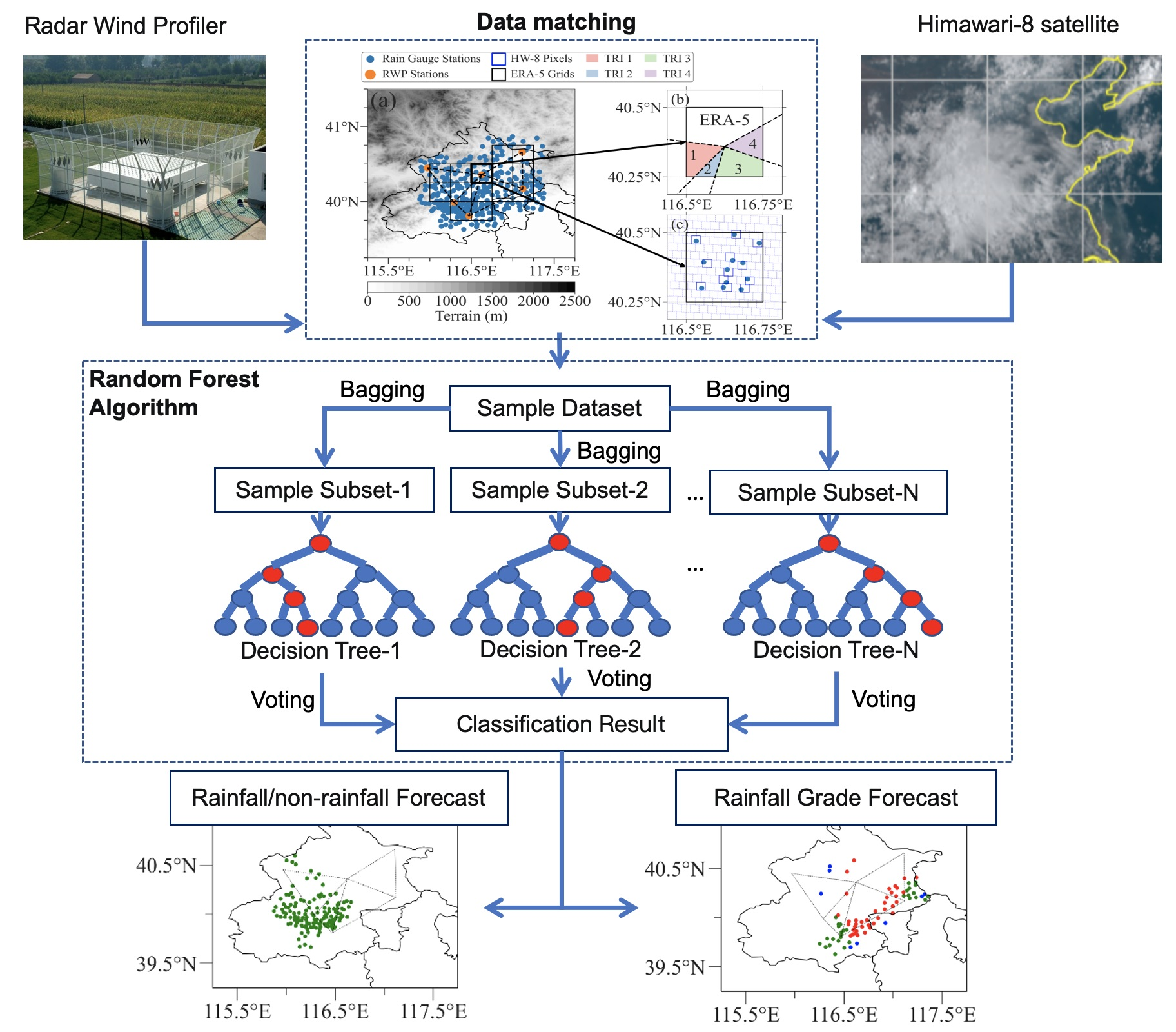
Figure 1a shows the spatial distribution of the RWP mesonet in Beijing, in which 4 triangles are formed. The well-recognized RWP triangular retrieving method, which was originally proposed by Bellamy [36], is used here to retrieve the profiles of divergence (D), vorticity (ξ), and vertical velocity (ω) within each triangle formed by the RWPs. The RWP data in the summers of 2018 and 2019 (June, July, and August) were selected for this study. According to the latitude and longitude of each vertex site of the triangle and the radius of the earth, the components of each side of the triangle in spherical coordinates (${\mathit{\Delta }x}_i,{\mathit{\Delta }y}_i,i=\mathrm{1,2},3$) are calculated. Then, the divergence (D) and vertical vorticity (ξ) at the same height are calculated by using the horizontal wind ($u_i,v_i,i=\mathrm{1,2},3$) measured with the RWPs at the vertexes. The formulae are as follows:

$$\left\{\begin{array}{c}D=\frac{(u_2-u_1)(\mathit{\Delta }{y}_3-\mathit{\Delta }{y}_1)-(u_3-u_1)(\mathit{\Delta }{y}_2-\mathit{\Delta }{y}_1)+(\mathit{\Delta }{x}_2-\mathit{\Delta }{x}_1)(v_3-v_1)-(\mathit{\Delta }{x}_3-\mathit{\Delta }{x}_1)(v_2-v_1)}{(\mathit{\Delta }{x}_2-\mathit{\Delta }{x}_1)(\mathit{\Delta }{y}_3-\mathit{\Delta }{y}_1)-(\mathit{\Delta }{x}_3-\mathit{\Delta }{x}_1)(\mathit{\Delta }{y}_2-\mathit{\Delta }{y}_1)}\\ \xi =\frac{(v_2-v_1)(\mathit{\Delta }{y}_3-\mathit{\Delta }{y}_1)-(v_3-v_1)(\mathit{\Delta }{y}_2-\mathit{\Delta }{y}_1)+(\mathit{\Delta }{x}_2-\mathit{\Delta }{x}_1)(u_3-u_1)-(\mathit{\Delta }{x}_3-\mathit{\Delta }{x}_1)(u_2-u_1)}{(\mathit{\Delta }{x}_2-\mathit{\Delta }{x}_1)(\mathit{\Delta }{y}_3-\mathit{\Delta }{y}_1)-(\mathit{\Delta }{x}_3-\mathit{\Delta }{x}_1)(\mathit{\Delta }{y}_2-\mathit{\Delta }{y}_1)}\end{array}\right.$$

(1)

The vertical velocity ω can be calculated by integrating the divergence in the vertical direction, according to the mass continuity equation. The calculation formula can be written as follows:

$$\omega =-{\int }_{P_0}^P\left(\frac{\partial u}{\partial x}+\frac{\partial u}{\partial y}\right)dp=-{\int }_{P_0}^{P}Ddp$$

(2)

2.2. Variables from Himawari-8 Satellite, ERA-5 Reanalysis and Rain Gauge

The Himawari-8 (HW-8), a new-generation geostationary satellite operated by the Japan Meteorological Agency, was launched on 7 October 2014 and has been able to provide observations with high spatial and temporal resolution (at 10 min) since 7 July 2015. The advanced Himawari imager (AHI) carried by the satellite has 16 channels [37], which can provide observations with different spatial resolutions (0.5–2 km) and central wavelengths (0.47–13.31 μm). Previous studies have shown that convective cloud systems can be accurately identified and tracked by using the cloud top brightness temperature observed by the infrared channel with a central wavelength of 10.4 μm and the reflectance observed by the visible channel with a central wavelength of 0.64 μm, so as to monitor the whole process of the occurrence, development, and extinction of convective cloud systems [25,38,39,40]. Therefore, the data from the two channels mentioned above are used as input features of the random forest model in this study, and both of them have a spatial resolution of ~2 km (0.02°) and temporal resolution of 10 min. This time range of the data includes the summers of 2018 and 2019 (June to August), covering the whole Beijing area.

ERA-5 reanalysis from the European Centre for Medium-Range Weather Forecasts (ECMWF) can provide a variety of environmental data with a temporal resolution of 1 h and a horizontal grid resolution of 0.25° × 0.25°, including using common convective parameters such as convective available potential energy (CAPE), the K index (also called George’s index), and the lift index (LI), which can be used to analyze large-scale environmental characteristics before the onset of convective weather [41]. While in practical application, the atmospheric environment data output from the NWP model is used [28,29]. In the vertical direction, ERA-5 provides reanalysis of air temperature, air pressure, humidity, and horizontal wind at 37 levels between 1000 and 10 hPa. In addition, the ERA-5 reanalysis provides divergence, vorticity, and vertical velocity data, which can be used to fill the area that cannot be covered by the triangular grid, so that the spatial matching of the mesh data of different shapes can be carried out (See Section 2.3 for more details). This study intends to use reanalysis data from the summers of 2018 and 2019 (June to August) in combination with other observational data as input features to the RF model. The ERA-5 data located within the rectangle ranging from 115.25°E to 117.75°E and from 39.25°N to 41.25°N are selected. Furthermore, this study will discuss the changes in the RF model performance when the divergence, vorticity, and vertical velocity features come from the reanalysis data as the source of the training dataset.

The rain gauge measurements from the surface synoptic station and automatic weather station throughout the whole Beijing region, which are operationally maintained by the China Meteorological Administration (CMA), are selected in this study. To temporally match the rain gauge with HW-8 observation, which has a temporal resolution of 10 min, cumulative precipitation within 10 min is calculated based on 1-min rainfall observations measured with rain gauges collected in the study area (Figure 1). All of these gauge measurements are obtained for the whole summers of 2018 and 2019 (June to August). Additionally, all of these precipitation measurements have been subject to strict data quality control.

2.3. Data Processing and Matching

In order to compare the forecast performance of the RF model using the gridded profile products of divergence (D), vorticity (ξ), and vertical velocity (ω) from the ERA-5 reanalysis as inputs, the triangular-averaged counterparts of atmospheric dynamic variables retrieved from RWP observations are converted into a grid of 0.25° × 0.25° to match the resolution of the ERA-5 reanalysis data. The area-weighted method is adopted to fill in D, ξ, and ω into each ERA-5 grid, which is schematically shown in Figure 1. The specific steps are as follows:

Firstly, according to the relative positions of the 4 triangles formed by 6 RWP stations in Beijing and ERA-5 grids, the overlap area (a_i) between the ith ERA-5 grid and its corresponding triangles is calculated, and then the weight (w_i) is assigned according to the ratio of overlap area ai to grid area (A_g), which is shown as follows:

$$w_i=\frac{a_i}{A_g}$$

(3)

where i denotes the ith ERA-5 grid overlapping with any number of triangles, as shown in Figure 1b.

Then, the weight W_RWP for all RWP triangles that overlap with a given ERA-5 grid is calculated, and the formula is as follows:

$$W_{\mathrm{RWP}}=\sum _{i=1}^4{w}_i$$

(4)

If the ERA-5 grid does not overlap with any triangles, namely if there are no RWP mesonet observational data on this grid, W_RWP will be equal to 0. When the W_RWP is equal to or greater than 10%, the ERA-5 grid is defined as an “observation grid”.

Finally, for each “observation grid”, the atmospheric dynamic variable (F_g), including D, ξ, and ω, was estimated by combining the component from the RWP observation (f_i) with the component from the ERA-5 reanalysis (f_era), according to the weights w_i and W_RWP. The formula is as follows:

$$F_g=(1-W_{RWP})\cdot f_{era}+\sum _{i=1}^4(w_i\cdot f_i)$$

(5)

In this way, f_i data are further converted into grid data with the same spatial resolution as the ERA-5 reanalysis by using the bilinear interpolation algorithm. Ultimately, we show the gridded D, ξ, and ω data for all grids in our study area in Figure 1, which is well matched with the satellite grid product from HW-8.

It should be noted that the ERA-5 data are stored in isobaric coordinates, while the RWP data are geometric coordinates. Therefore, to match the RWP-retrieved D, ξ, and ω with ERA-5 reanalysis data in the vertical, the geometric height of the RWP variables have been transformed to isobaric height using the hypsometric equation and then the linear interpolation method is applied. On this basis, the rain gauge station closest to each satellite pixel is selected to obtain rainfall for this satellite pixel, which is schematically demonstrated in Figure 1c. If a pixel does not match any of the gauge stations, the sample is dropped. If there is more than one station in the same pixel, the rainfall data of these stations are averaged, ensuring a one-to-one correspondence between the satellite pixel and the rainfall data. Finally, all of these data are matched well with each other in accordance with time, which lays a solid dataset foundation for the ensuing RF modeling and evaluation, as shown in

Table 1. The data sources of feature variables used as inputs for the RF modeling.

Data Source	Temporal Resolution	Feature Name	Units
ERA-5 reanalysis	60 min	Convective Available Potential Energy	J·kg−1
		Convective Inhibition	J·kg−1
		K Index	°C
		Surface Pressure	hPa
		Temperature	°C
		2 m Dewpoint Temperature	°C
		Zero Degree Level	m
		Total Totals Index	°C
		Precipitable Water	mm
		u-component and v-component wind	m/s
		Relative Humidity	%
Radar wind profiler (RWP)	6 min	Vorticity	s−1
		Divergence	s−1
		Vertical Velocity	Pa·s−1
Himawari-8 (HW-8)	10 min	10.4 μm Brightness Temperature	K
		0.64 μm Albedo	non-dimensional
Rain gauge	10 min	Precipitation	mm

.

Here, only HW-8 pixels paired with a gauge station are selected as input samples. Meanwhile, to make full use of the RWP observation data in modeling and to ensure sufficient samples for modeling, sample points are also selected according to the following criteria: (1) pixels should be located inside the observation grid; (2) there is at least one observation grid around the pixel, even if its position does not meet Condition (1). By this way, 300 plus sample pixels are selected in our study area.

Meanwhile, the precipitation events used in this study are required to meet the following criteria: (1) the average rainfall rate of all samples in the study area is greater than or equal to 0.1 mm/10 mins from a certain time and lasts for more than 30 min; (2) the interval time of the adjacent rainfall process is greater 120 min; (3) the onset time of a rainfall event is defined as the moment (i.e., t = 0) that the average rainfall of the samples firstly reaches 0.5 mm/10 mins.

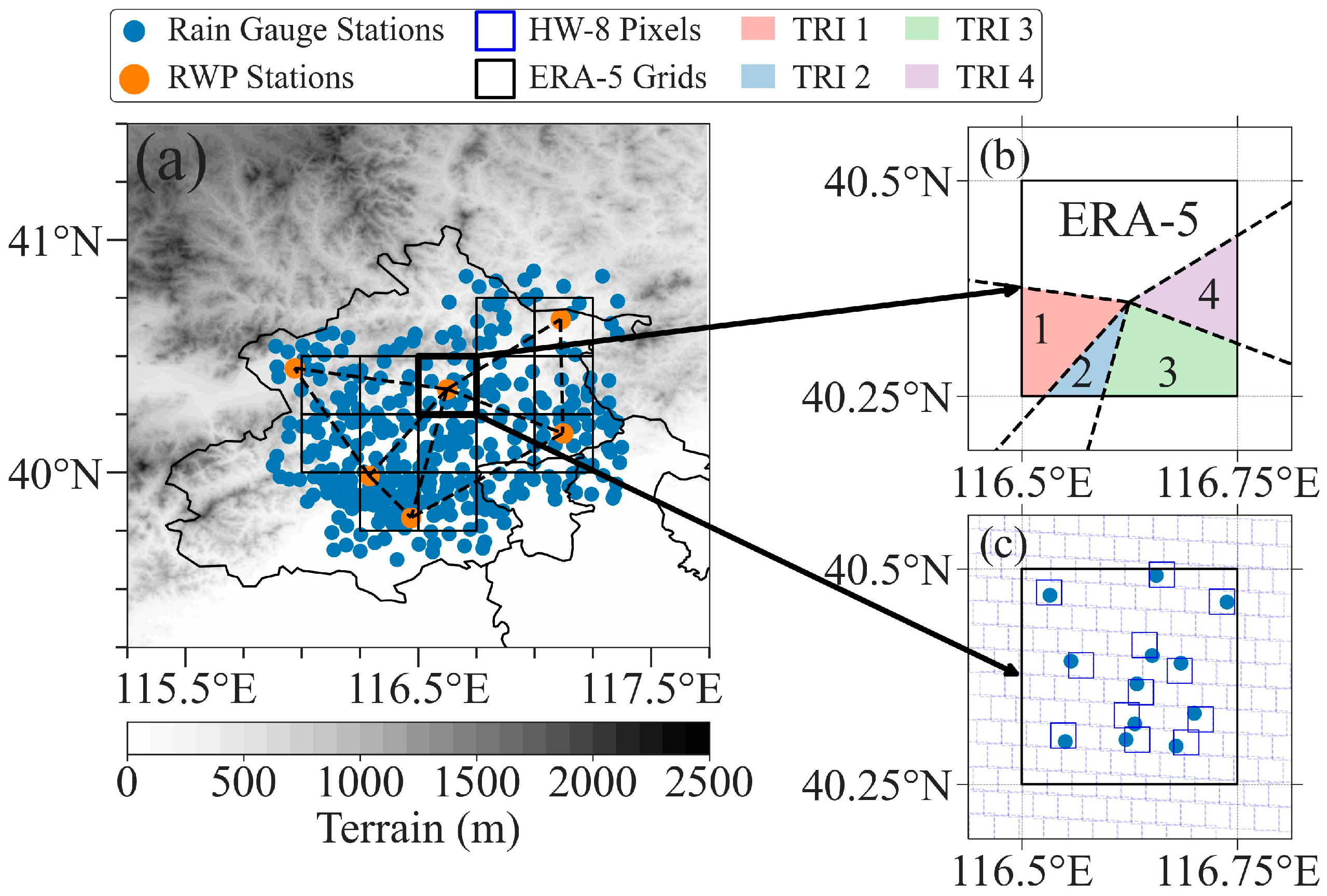
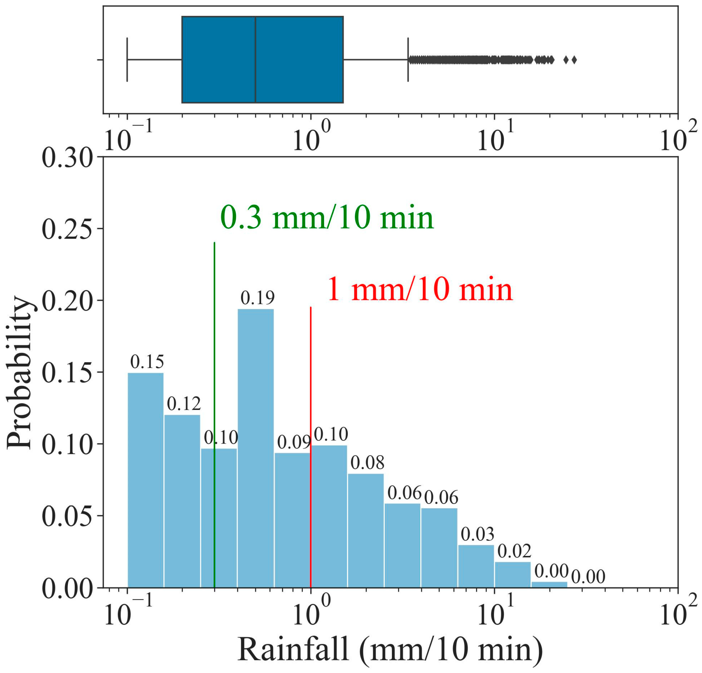
Then, three rainfall grades are defined by the observed precipitation (rainfall) probability distribution of all rain gauges in the study area during the summers of 2018 and 2019, which is presented in Figure 2. According to this probability distribution, all of the rainfall samples are divided into three terciles. In particular, the lowest tercile (rainfall ≤ 0.3 mm) is deemed to be light rain, the middle tercile (0.3 mm ≤ rainfall < 1 mm) to be moderate rain, and highest tercile (rainfall ≥ 1 mm) to be heavy rain.

Prior to performing the temporal match of the input dataset, the latency of the various datasets used in this study needs to be clarified. HW-8 has a temporal resolution of 10 min, but the transmission of the HW-8 satellite data needs 5–10 min, leading to a significant time delay. The RWP can be available in real time at 6-min intervals. Here, we merely carry out the 30-min nowcasting of rainfall. Therefore, the 30-min HW-8 satellite measurements correspond to the period from −40 to −10 min before the onset of rainfall, and the 30-min RWP observational data correspond to the period from −42 min to −12 min before the onset of rainfall. For example, the HW-8 data corresponding to 20 min before rainfall (t = −20) is generally matched with the RWP data corresponding to 24 min before precipitation (t = −24). All of these observational data from both HW-8 and RWP are further matched with the atmospheric environmental variables from the hourly ERA-5 reanalysis data, which is implemented by using the linear interpolation method. At the end of the day, we prepared the dataset for RF modeling based on a muti-source dataset with various spatial and temporal resolutions, including satellite observation, RWP observation, and ERA-5 reanalysis. Given no analysis field or operational forecasting meteorological field are available for us in this study, we had to resort to ERA-5 reanalysis data, which cannot always be available. Note that in the future, in the rainfall nowcasting operation, we can take in the analysis field or forecasting meteorological field in the operational rainfall nowcasting model.

2.4. The Random Forest Classification Algorithm

2.4.1. Random Forest Classifier

In the classification task, the RF algorithm can take the optimal estimator with the highest voter turnout as the output result for the final model, according to the voting result of each decision tree on the input samples and the principle of minority obedience to majority.

The RF algorithm adopts a random sampling method with a bagging regression method, which ensures the scientific nature of each decision tree model from a statistical point of view [42]. In addition, since there are unused out-of-the-bag (OOB) samples in the training processes of the RF model, the OOB samples can be used as verification set samples during the training process in order to evaluate the accuracy of the prediction classification or regression of the random forest model. When the number of trees is sufficient, the OOB score can be used as an unbiased estimation method for model accuracy [43,44].

The scikit-learn class library based on Python language is a common machine learning module that integrates the basic functions of random forest model training, parameter optimization, and prediction, and provides several evaluation indicators to evaluate the model performance. It is noteworthy that the widely used “Random Forest Classifier” method has been used to implement the random forest classification algorithm (https://scikit-learn.org/stable/, accessed on 16 March 2023).

2.4.2. Training Process

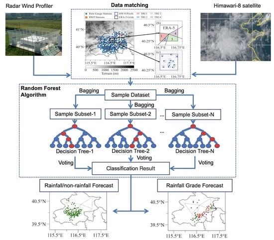
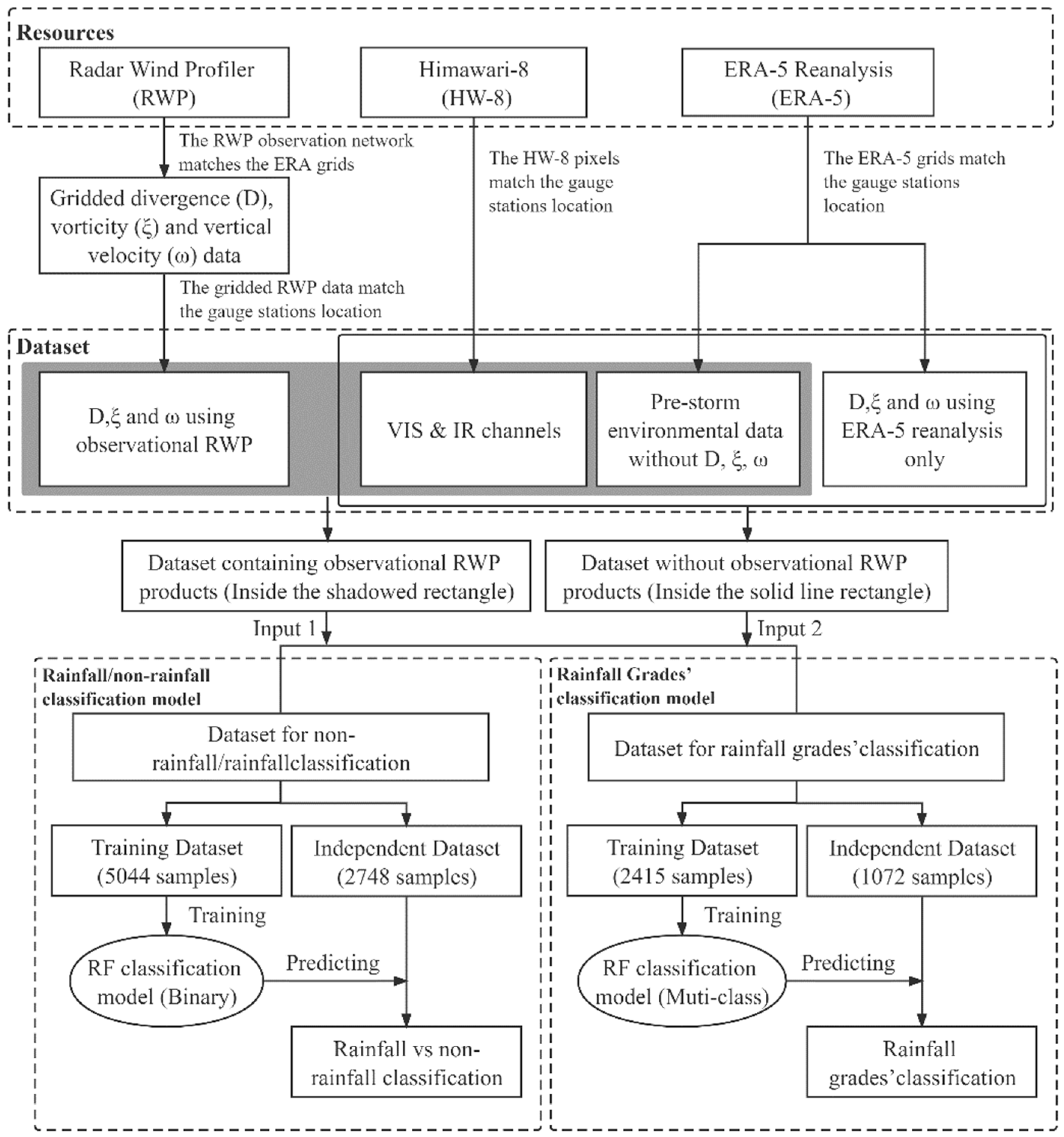
This study intends to develop a set of rainfall forecast and rainfall grade forecast algorithms based on the RF classification model, and the technical flow chart is shown in Figure 3.

After the temporal-spatial matching and interpolation of the modeling dataset, the rainfall events in the summer of 2019 (from June to August) are selected as the training set. The RF binary classification model is used for the forecast of rainfall/non-rainfall, which labels the samples with no rainfall as 0 and those with rainfall as 1. For the rainfall grade forecast, the RF muti-class classification model is adopted, after removing the samples without rainfall in the modeling dataset and defining the sample labels according to the rainfall grades divided in Section 2.3. The training of the above two RF classification models is independent. In this step, the correlation coefficient between each feature in the training set and rainfall is calculated first, and the optimal feature subset is selected by the backward sequence selection method based on the feature importance score of the RF model. Then, the grid search method is used to adjust the hyperparameters of the model to obtain the optimal RF classification model. Finally, the trained forecast model is applied to the independent dataset (from June to August 2018).

When the independent dataset is used to evaluate the model, the evaluation data within 30 min before the rainfall initiates are selected, which are then taken as inputs into the model with a resolution of 10 min. It is intended to predict whether rainfall occurs at different lead times (i.e., −40, −30, −20, and −10 min). In addition, these datasets are used to predict different grades of rainfall, including light rain, moderate rain, and heavy rain. In addition, the differences in the forecast performance of the two models are evaluated when the atmospheric dynamic variables, including D, ξ, and ω, are from ERA-5 reanalysis instead of RWP retrievals.

For the sake of simplicity, the RF classification model for rainfall/non-rainfall forecast, which uses RWP data as the source of D, ξ, and ω features, is dubbed as the binary RWP model, whereas the rainfall grade forecast model is named as the muti-class RWP model. Similarly, by changing the input dataset from RWP to ERA-5 reanalysis, the models become a binary ERA-5 model and a muti-class ERA-5 model.

2.5. Accuracy Evaluation

For the rainfall/non-rainfall forecast, the confusion matrix commonly used in binary models is used in the present study to calculate the difference between the forecast output of the model and the actual label of the sample. On this basis, the performance of the model is evaluated by further calculating the well-established metrics, including the false alarm ratios (FAR), probability of detection (POD), and accuracy, all of which are three commonly used test metrics for weather forecasting. In addition, the threat score (TS) and the equitable threat score (ETS) are used. The calculation formulae of the above five metrics are given as follows:

$$FAR=\frac{FP}{TP+FP}$$

(6)

$$POD=\frac{TP}{TP+FN}$$

(7)

$$Accuarcy=\frac{TP+TN}{TP+TN+FP+FN}$$

(8)

$$TS=\frac{TP}{TP+FP+FN}$$

(9)

$$ETS=\frac{TP-Dr}{TP+FP+FN-Dr}$$

(10)

$$Dr=\frac{(TP+FP)(TP+FN)}{TP+TN+FP+FN}$$

(11)

where TP represents the number of observed samples and predicted results that are positive; FN represents the number of observed samples that are positive and predicted results that are negative; FP represents the number of observed samples that are negative and predicted results that are positive; and TN represents the number of observed samples that are negative and predicted results that are also negative.

In the binary classification problem, the output label of the RF model is the judgment probability of the model for each type of label, and setting different probability thresholds will lead to different output results and thus obtain different confusion matrices. Therefore, this paper adopts the metric of the area under the curve (AUC) to evaluate the performance of the model under different probability thresholds.

For the rainfall grade forecast based on the multi-class RF classification model, we take each classification label as the benchmark and mark the output result of the model and the sample label as “True”, otherwise it is “False”. The confusion matrix is applied to the multi-classification label test in this “one-to-many” way, and then the evaluation index of each label is calculated. Since the accuracy rate is expressed as the proportion of samples correctly classified, this indicator is used to evaluate the overall performance of the magnitude prediction model for all labels.

3. Results and Discussion

3.1. Correlation Analysis between Atmospheric Dynamic Variables from RWP and Rainfall

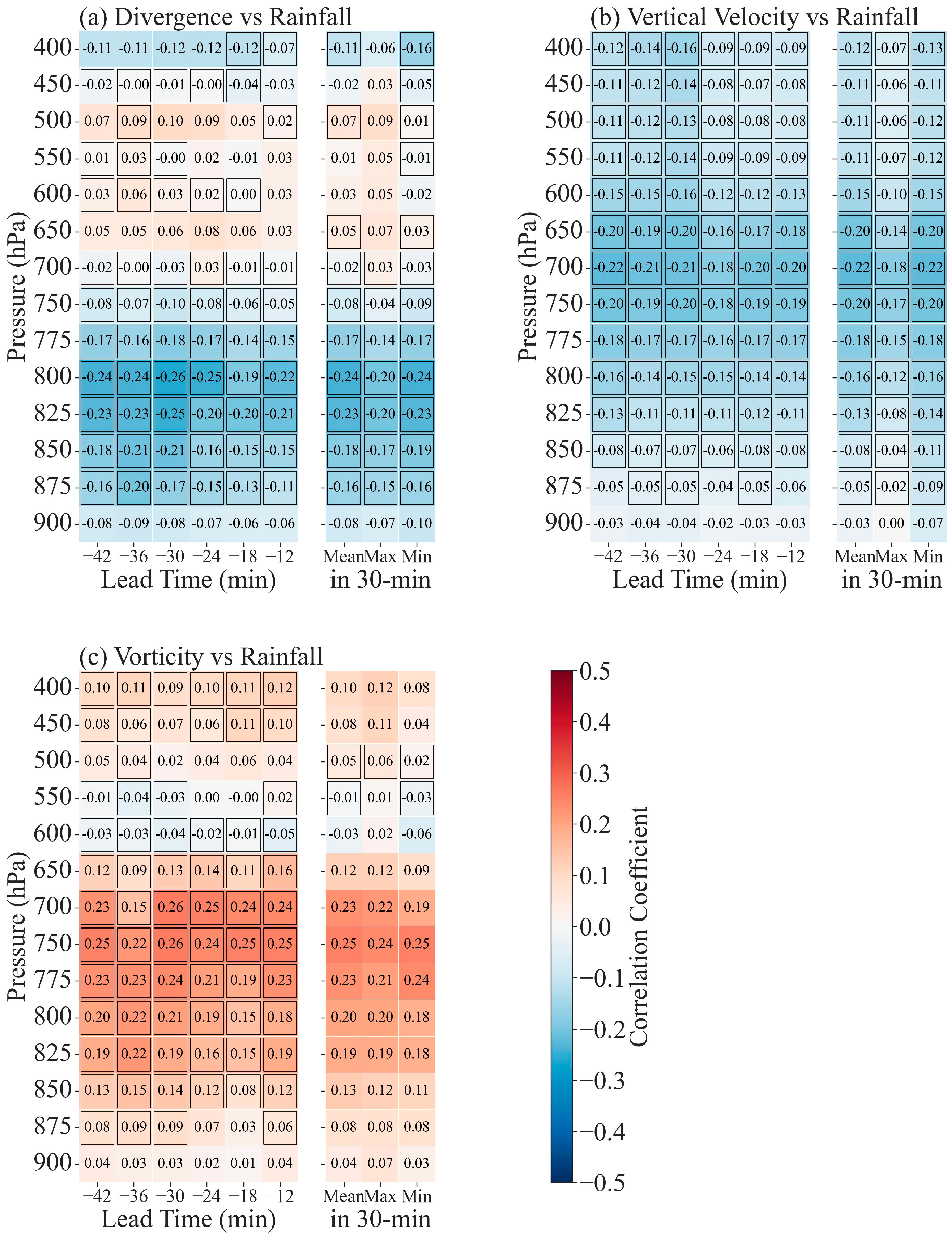
Given the huge uncertainties of the RWP retrievals of atmospheric dynamic features near the rainfall onset, the divergence, vorticity, and vertical velocity based on the RWP measurements at 6-min intervals are selected for the period from t = −42 to t = −12 min. Then, the time-lagged Spearman correlation coefficient matrices between the rainfall samples at the beginning of rainfall (t = 0) and the atmospheric dynamic feature at each level are calculated. Additionally, the correlations between the rainfall and the mean, maximum, and minimum of those features in the first 30 min are calculated.

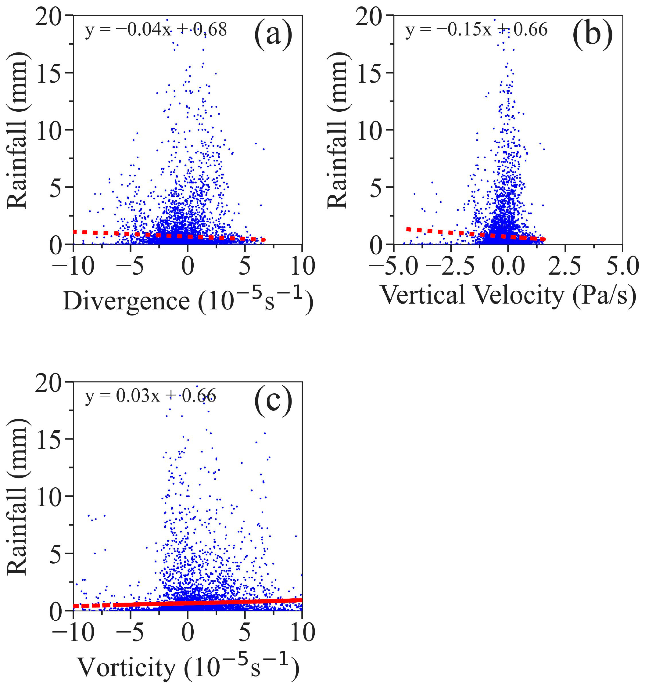
Figure 4a shows the correlation coefficient between the divergence profile and rainfall. Interestingly, a negative correlation is found at the pressure levels starting from the ground surface up to 700 hPa, and a positive correlation is found between 700 hPa and 500 hPa. The negative correlation is larger at the lower level, from 775 hPa to 875 hPa. For the vertical velocity (Figure 4b), the correlation coefficient is negative. Additionally, the correlation coefficient becomes positive for most of the pressure levels between the vorticity profile and rainfall (Figure 4c). The levels with larger absolute values of correlation coefficients are basically consistent with the divergence profiles, but the symbols are the opposite. Overall, the vertical velocity presents a negative correlation (Figure 4b), in which the levels with a larger absolute value of correlation coefficients are distributed in the middle levels, from 650 hPa to 750 hPa. As shown in Figure 5, the pre-storm divergence and vertical velocity are negatively associated with rainfall, and vorticity is found to be positively associated with rainfall. Positive vorticity favors the formation of cyclone circulation, and thus the increase in positive vorticity tends to provide an environment that is favorable for the rainfall onset.

Based on the analysis of the correlation coefficient, we select the levels where the absolute values of the correlation coefficient between the mean value of each variable and rainfall are equal or greater than 0.2. It follows that the divergence at 800 hPa and 825 hPa; the vertical velocity at 650 hPa, 700 hPa, and 750 hPa; and the vorticity at 700 hPa, 750 hPa, 775 hPa, and 800 hPa are the ultimate potential features. This to some extent justifies the necessity to use the input variable from the RWP mesonet observations.

3.2. Influence of Different Input Features on RF Model Performance

The optimal feature subset refers to the data subset that is extracted from the original variable dataset, which is further used for the development of classification or regression models in an attempt to achieve a similar or an even better estimation accuracy than using the original variable [45]. Finding the optimal feature subset is one of the most important issues in feature engineering. Its purpose is to remove the irrelevant or redundant features in an attempt to simplify the model, to improve the accuracy of the model, and to reduce the running time.

The feature importance ranking function of the RF model can be used to determine the optimal feature subset. The backward selection method is adopted here. The specific process is as follows: First, the importance of all of the features determined in Section 3.1 is calculated and sorted, as shown in

Table 2. The list of the input features of the RF models used in rainfall/non-rainfall forecast (binary) and rainfall grade forecast (multi-class). Note that the removal order of each undetermined feature is determined by the feature importance score of the RF model, and the removal order of features with a low score was the first. The optimal feature subsets of binary and multi-class prediction models determined by the backward sorting method are the features without asterisk (*).

Data Source	Feature Name	Descriptions	Remove Order
			Binary	Multi-Class
ERA-5 reanalysis	CAPE	Convective Available Potential Energy	18	18
	DEG0L	Zero Degree Level	7	10
	KX	K Index	14	21
	LI	Lifting Index	1 *	2 *
	MUCAPE	Most Unstable Convective Available Potential Energy	13	5
	PW	Precipitable Water	20	20
	R_550	Relative Humidity on 550 hPa	17	15
	θse_800	Potential Pseudo-Equivalent Temperature on 800 hPa	22	19
	SHR_1-0	0–1 km Wind Shear	8	12
	T_400	Temperature on 400 hPa	19	14
	TOTALX	Total Totals Index	9	13
Himawari-8 (HW-8)	IR	10.4μm Brightness Temperature	21	17
	VIS	0.64μm Albedo	5 *	1 *
Radar wind profiler (RWP)	D_800	Divergence on 800 hPa	12	22
	D_825	Divergence on 825 hPa	10	9
	VO_700	Vorticity on 700 hPa	16	11
	VO_750	Vorticity on 750 hPa	4 *	3 *
	VO_775	Vorticity on 775 hPa	2 *	7
	VO_800	Vorticity on 800 hPa	11	16
	W_650	Vertical Velocity on 650 hPa	3 *	8
	W_700	Vertical Velocity on 700 hPa	6 *	4
	W_750	Vertical Velocity on 750 hPa	15	6

. Then, starting from the features with the least importance, the features of the undetermined feature set are deleted successively in order to build the RF model until only two variables remain in the undetermined features. Finally, the prediction accuracy of the RF model is evaluated according to the evaluation index of the RF model in each cycle (i.e., the OOB score). The subset corresponding to the small number of variables and the high prediction accuracy of the model is taken as the optimal subset, that is, the result of variable selection.

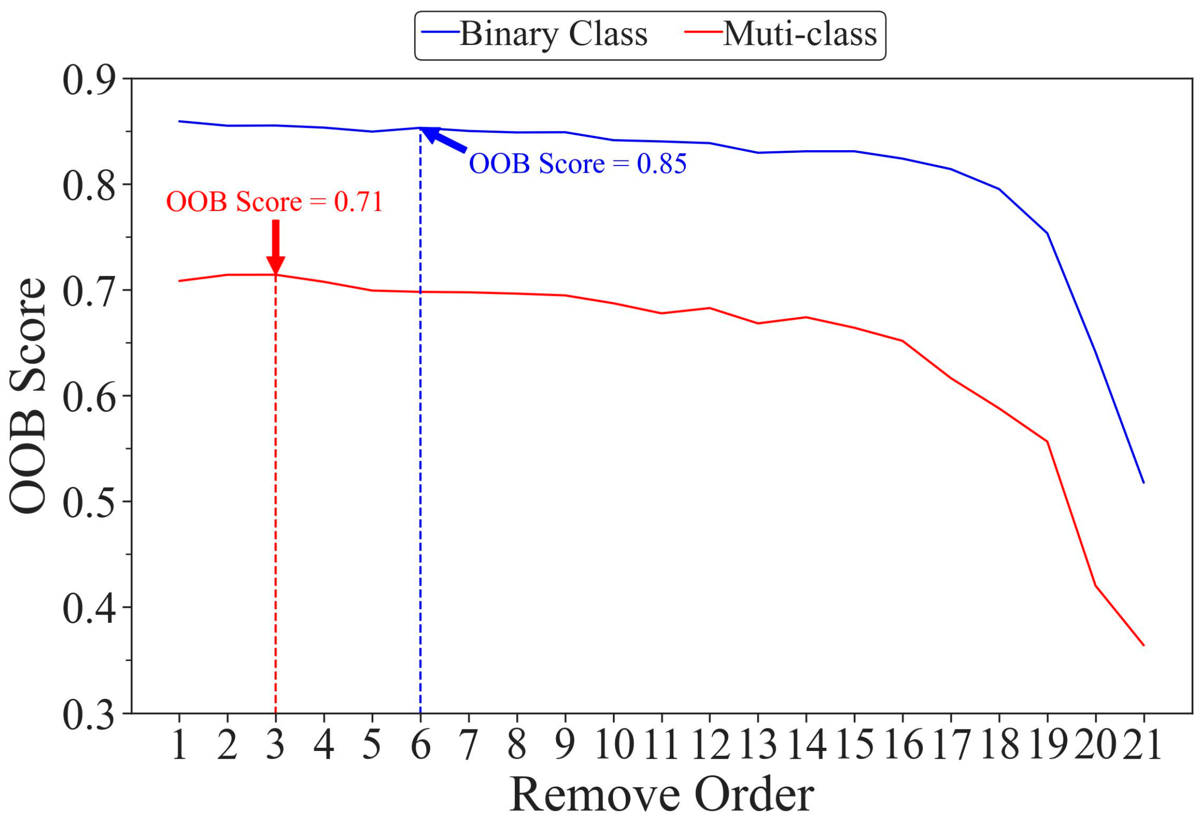
The OOB scores corresponding to the input feature selection process of the two RF models are shown in Figure 6. For the binary classification RF model (used for the rainfall/non-rainfall forecast), when the first six features are removed in the order that is shown in Table 2, the OOB score of the model changes little compared with that before the removal. However, when the features are removed from the original feature set, the OOB score begins to decline. For the muti-class classification RF model (used for the rainfall grade forecast), the OOB score reaches its highest when the first three features are removed from the undetermined feature set, and then the OOB score decreases with the removal of the features. Note that the selected feature subset refers to those features without an asterisk in Table 2.

3.3. Hyperparameter Optimization

Hyperparameter tuning (or hyperparameter optimization) is the process of determining the correct combination of hyperparameters that maximizes the model performance. It runs multiple tests in one training session. Each trial is a complete execution of the training program, and the hyperparameter setting values are selected within a specified range. This process, once it is completed, will give a set of hyperparameter values that best fit the model for optimal results. For the RF algorithm, the out-of-pocket samples can be used as the validation data set, and the model performance can be evaluated during training.

After determining the optimal feature subset, we use the grid search method to arrange and combine the hyperparameter values of the model and build models one by one according to these combinations. After that, the optimal hyperparameters are determined according to the performance (measured by the OOB score in this paper) of these models in the verification set (the out-of-bag samples). The undetermined hyperparameters and their undetermined value ranges are shown in

Table 3. Descriptions for the undetermined hyperparameters for the binary RF model and muti-class RF model used for rainfall forecast. For the max_features, ‘sqrt’ indicates that the value is the square root of the number of features, ‘log’ indicates that the value is the logarithm of the number of features, and ‘None’ indicates no restriction.

Hyperparameter Name	Descriptions	Adjusting Range	Values of Selected Parameters
			Binary	Muti-Class
n_estimators	The number of trees in the forest.	10, 50, 90, 100, 200, 300, 500, 800, 1000	300	200
max_depth	The maximum depth of the tree.	5, 8, 15, 25, 30, None	8	5
min_samples_leaf	The minimum number of samples required to be at a leaf node.	1, 2, 5, 10	5	1
min_samples_split	The minimum number of samples required to split an internal node.	2, 5, 10, 15	2	5
max_features	The number of features to consider when looking for the best split.	sqrt, log, None	sqrt	None

. The hyperparameter optimization is carried out based on the blended dynamic variables from ERA-5 reanalysis and RWP measurements, which is executed separately for the binary and muti-class classification RF model. When the input data changed to ERA-5 reanalysis, no further adjustment has been made in hyperparameter optimization.

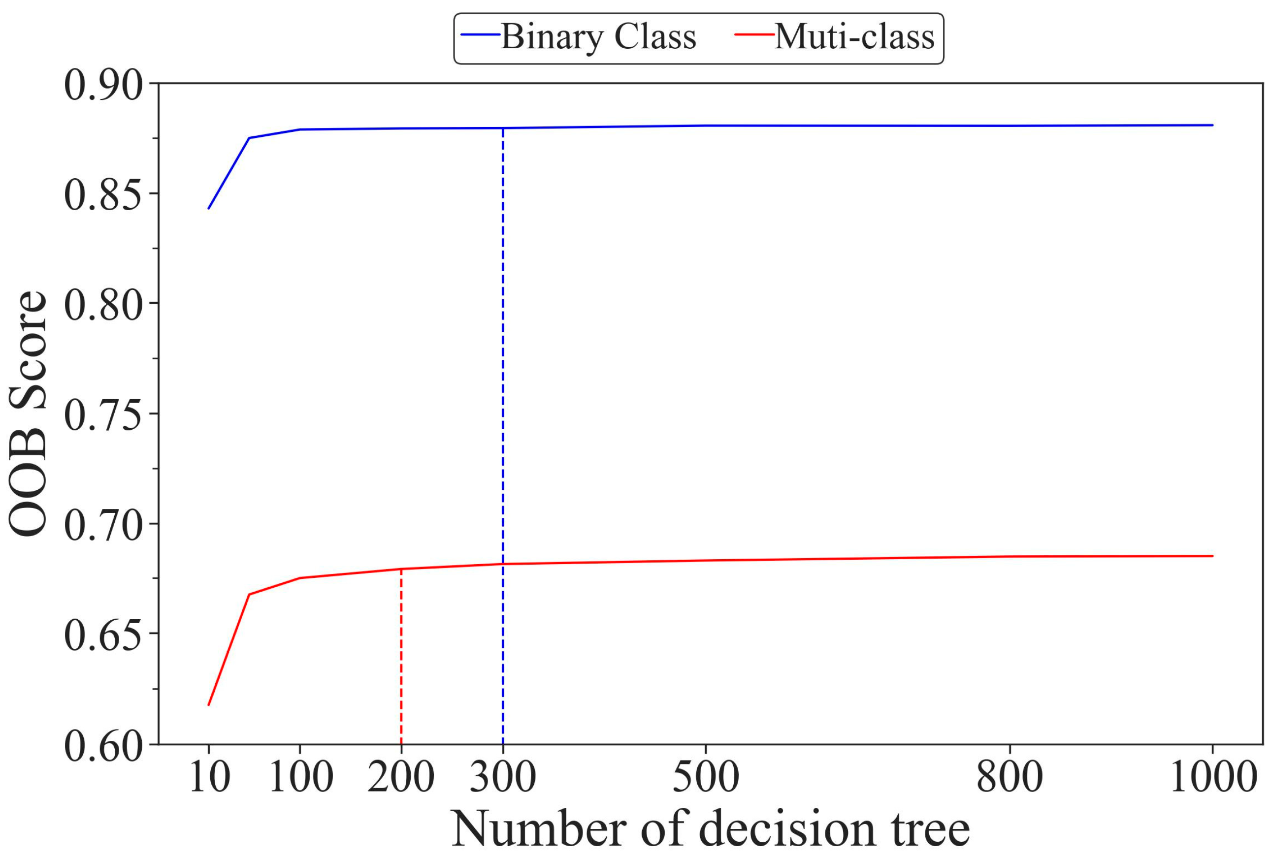
Figure 7 shows the OOB scores of the binary model (blue line, used for the rainfall/non-rainfall forecast) and the muti-class model (red line, used for the rainfall grade forecast) change with the total number of decision trees. At the beginning, the OOB score increases with the increase in the number of decision trees in the model, and the model performance is continuously optimized. However, after reaching a certain level, the OOB scores level off, indicating that the model accuracy is barely improved. Correspondingly, the amount of computation consumed by the model is increasing. Considering the balance between the performance and the complexity of the model, the total number of decision trees of the model that is used for the rainfall/non-rainfall forecast in this study is set to 300, and that of the model that is used for the rainfall grade forecast is set to 200. The rest of the hyperparameter settings are shown in Table 3.

3.4. The Feature Importance Scores of the Input Features from Different Data Sources

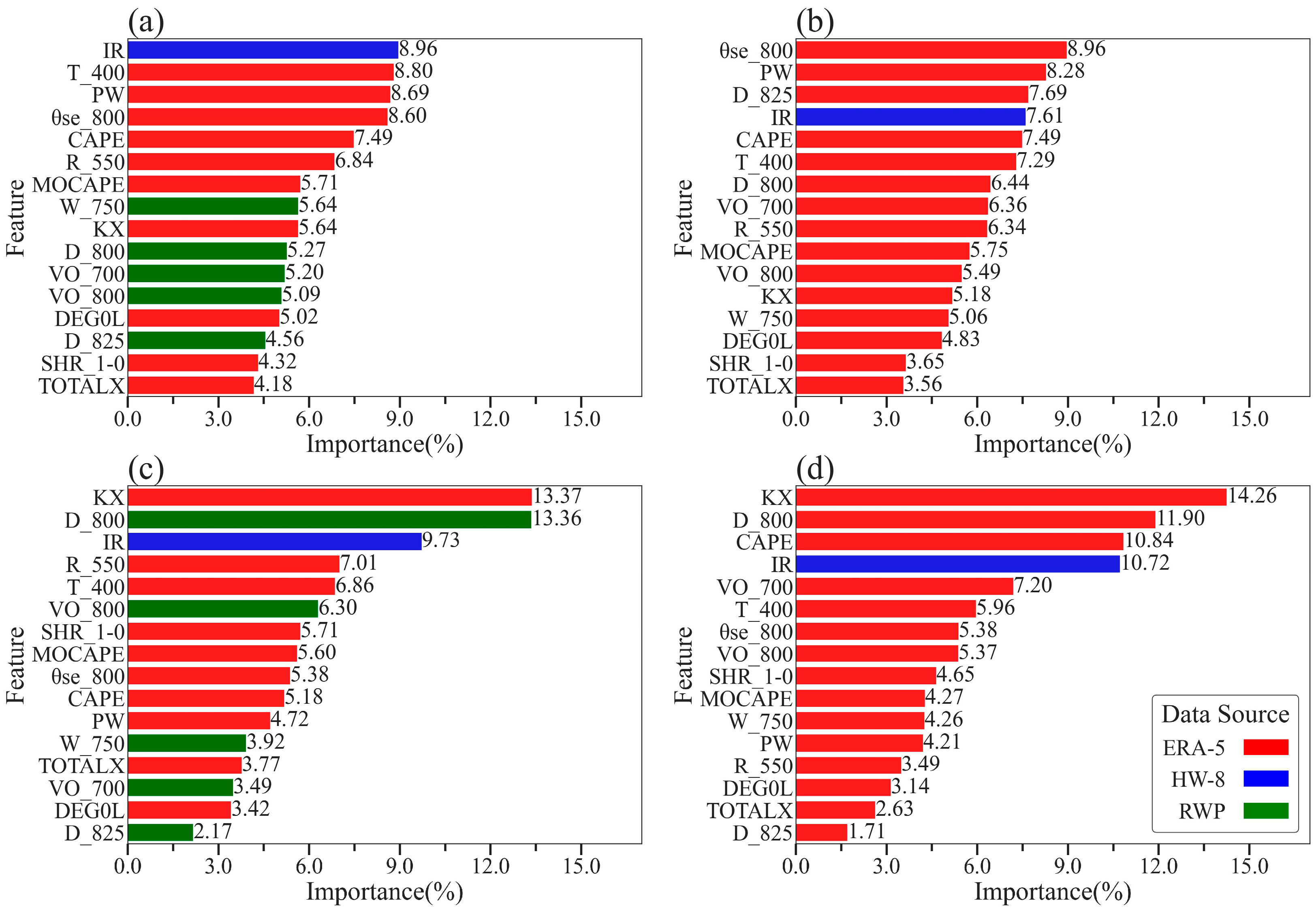
The ranking lists of the feature importance scores in the rainfall/non-rainfall forecast and the rainfall grade forecast are shown in Figure 8. As presented in Figure 8a, where the input features of D, ξ, and ω for the binary RF model are obtained from RWP measurements, the importance scores of each input feature are roughly ranked from high to low as geostationary satellite data, the thermodynamic features based on ERA-5, and the dynamic features based on RWP observation, with the 0–1 km wind shear and total index using ERA-5 ranking last. When the input features of D, ξ, and ω are from ERA-5 reanalysis, with the rest of the input features unchanged, the scores of the divergence at 825 hPa and 800 hPa (4.56% vs. 7.69%, 5.27% vs. 6.44%) and vorticity at 800 hPa and 700 hPa (5.09% vs. 5.49%, 5.20% vs. 6.36%) increase, while the score of the vertical velocity at 750 hPa decrease (Figure 8b). For the rainfall grade forecast (Figure 8c,d), when ERA-5 reanalyses are used as the data source, the importance score of the vorticity at 700 hPa increases from 3.49% to 7.20%, compared with the observation data, as does the importance score for the vertical velocity at 750 hPa. Conversely, the vorticity at 800 hPa shows a significant decrease in importance score. For the divergence at 800 hPa and 825 hPa, their ranking does not change relative to the other characteristics, although their importance scores decrease when the data source is changed.

For the other features in Table 2 that use ERA-5 as data sources, the importance scores of some features change greatly when they are combined with the divergence, vorticity, and vertical velocity features of different data sources as input features. When the D, ξ, and ω characteristics change from observational data to ERA-5 data, the relative humidity on 550 hPa in the rainfall forecast decreases (7.01% vs. 3.49%), and the importance score of CAPE increases (5.18% vs. 10.84%). However, the feature importance score of CAPE does not change in the rainfall/non-rainfall forecast. There are significant changes in the pseudo-equivalent potential temperature at 800 hPa (8.60% vs. 8.96%), temperature t 400 hPa (8.80% vs. 7.29%), relative humidity at 550 hPa (6.84% vs. 6.34%), and K index (5.64% vs. 5.18%). As for the satellite features, whether the combination of D, ξ, and ω features from any data source are used as model inputs, its feature importance scores rank the highest.

Compared with the rainfall/non-rainfall forecast, the feature importance scores of divergence and vorticity at 800 hPa in the rainfall grade forecast model are higher, while the importance scores of ω at 750 hPa, ξ at 700 hPa, and D at 825 hPa are lower than those in the rainfall/non-rainfall forecast. For the other features that only use ERA-5 as a data source, the importance of the K index and 0–1 km wind shear in the rainfall grade forecast is much higher than that in the rainfall/non-rainfall forecast; however, CAPE, precipitable water (PW), and the pseudo-equivalent potential temperature at 800 hPa decline in the rainfall/non-rainfall forecast.

3.5. Independent Dataset Evaluate Results

3.5.1. Evaluation of Rainfall/Non-Rainfall Forecast

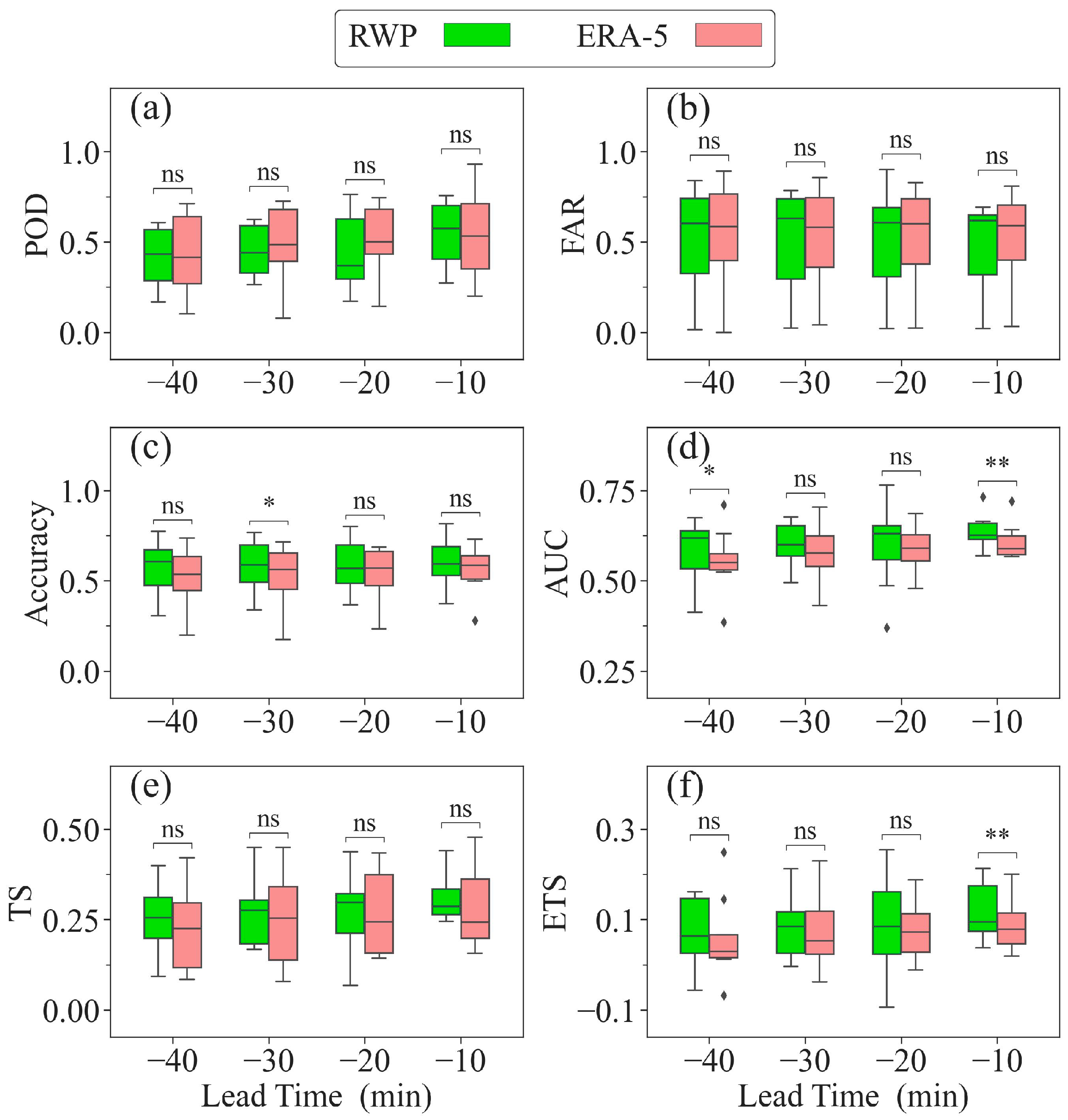
The criteria in Section 2.5 are used to evaluate the performance of the rainfall/non-rainfall forecast based on the RF model using RWP observational data (binary RWP model) and ERA-5 reanalysis (binary ERA-5 model). The samples for evaluation are selected within 30 min before the onset of each rainfall process (i.e., t = −40–−10 min). Then, the boxplot is drawn according to the score distribution of each process, which is demonstrated in Figure 9.

Figure 9a shows that the probability of detection (POD) at t = −30 and t = −20 min resulting from the forecast that is based on the binary ERA-5 model is slightly higher than the one that is based on the binary RWP model. In terms of false alarm ratios (FAR) for the rainfall/non-rainfall forecast, the binary RWP model outperforms the binary ERA-5 model for its relatively low scores within 30 min before the onset of rainfall (Figure 9b). The use of RWP in the RF model also results in a much better performance for a much higher accuracy score (Figure 9c), AUC score (Figure 9d), and ETS (Figure 9f). This suggests that the binary RWP model has advantages in rainfall/non-rainfall forecast, compared to the binary ERA-5 model. Nevertheless, for the TS score (Figure 9e), the median score of the binary RWP model is higher than the binary ERA-5 model, and the binary ERA-5 model has a higher TS score for some rainfall cases, therefore, the maximum score is better than that of the binary RWP model. Overall, the binary RWP model performs on average much better than the binary ERA-5 model.

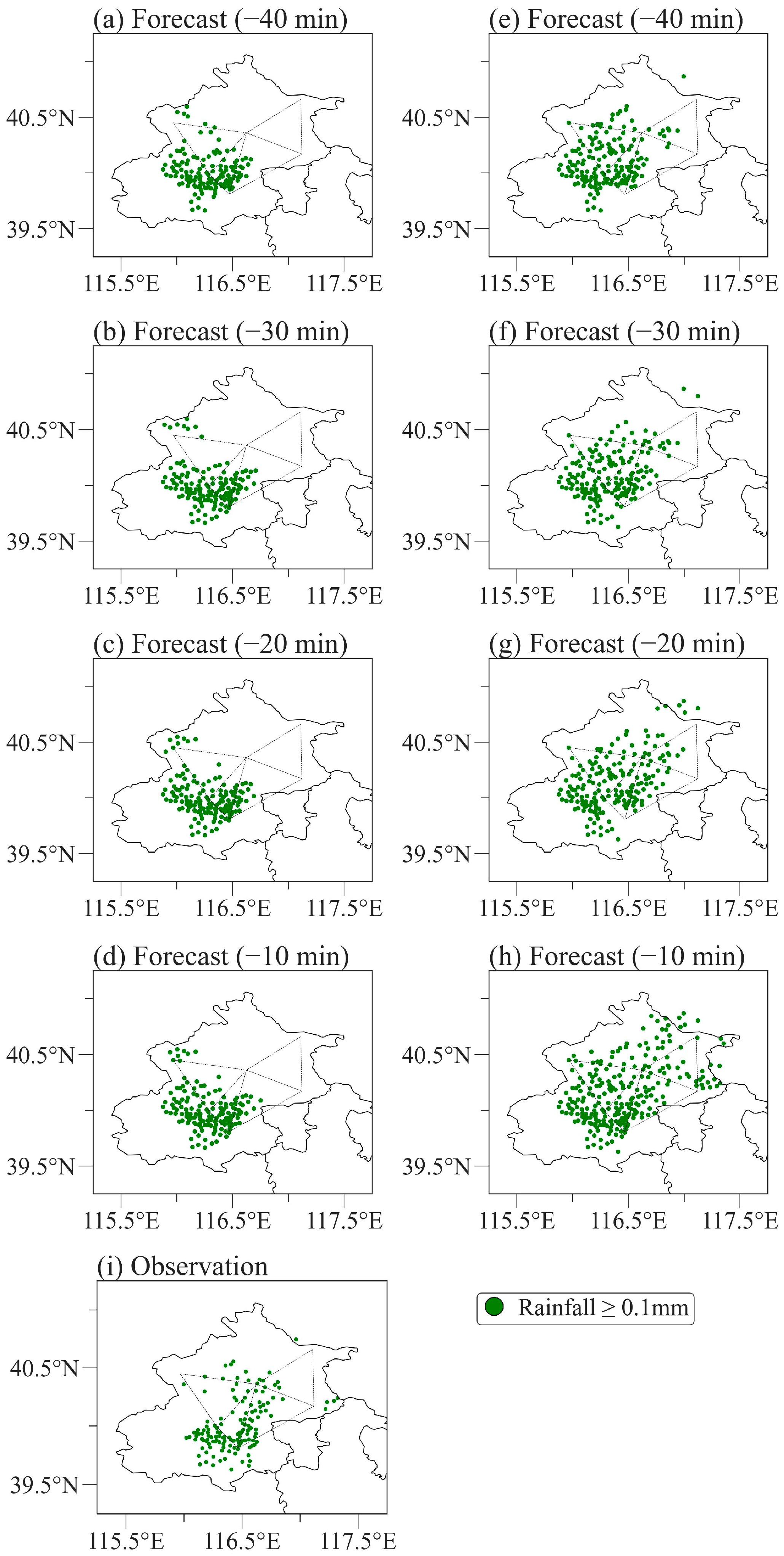
A case in point for the mode performance is shown in Figure 10 by using different input atmospheric dynamic variables. This rainfall event begins at 23:20 BJT on 16 July 2018. The binary RWP model can well forecast the areas with rainfall in the southwest of Beijing, while for the central and northern areas with sparse rainfall, the model misses it. By comparison, the forecast from the binary ERA-5 model produces rainfall in almost all of the stations, which cannot reflect the whole picture of this rainfall process. According to the criteria that are listed in

Table 4. Summary of the performance metrics of the RF model used to carry out the rainfall/non-rainfall forecast within 30 min before the rainfall onset at 23:20 BJT on 16 July 2018.

Data Source	Lead Time (min)	FAR	POD	Accuracy	AUC	TS	ETS
RWP	−40	0.42	0.56	0.65	0.64	0.40	0.16
	−30	0.38	0.62	0.68	0.68	0.45	0.21
	−20	0.40	0.62	0.67	0.66	0.44	0.20
	−10	0.41	0.63	0.63	0.66	0.44	0.19
ERA-5	−40	0.46	0.64	0.63	0.63	0.42	0.15
	−30	0.44	0.69	0.65	0.66	0.45	0.18
	−20	0.46	0.70	0.63	0.64	0.43	0.15
	−10	0.49	0.89	0.60	0.64	0.48	0.15

, the accuracy, AUC, and ETS scores of the binary RWP model in this case are better than the binary ERA-5 model for each lead time. There are no significant differences in the TS scores between the two data sources for the rainfall/non-rainfall forecast at the lead times of 30 and 20 min; however, the binary RWP model is superior to the binary ERA-5 model at the lead time of 40 min, while the reverse is true for the lead time of 10 min.

3.5.2. Evaluation of Rainfall Grade Forecast

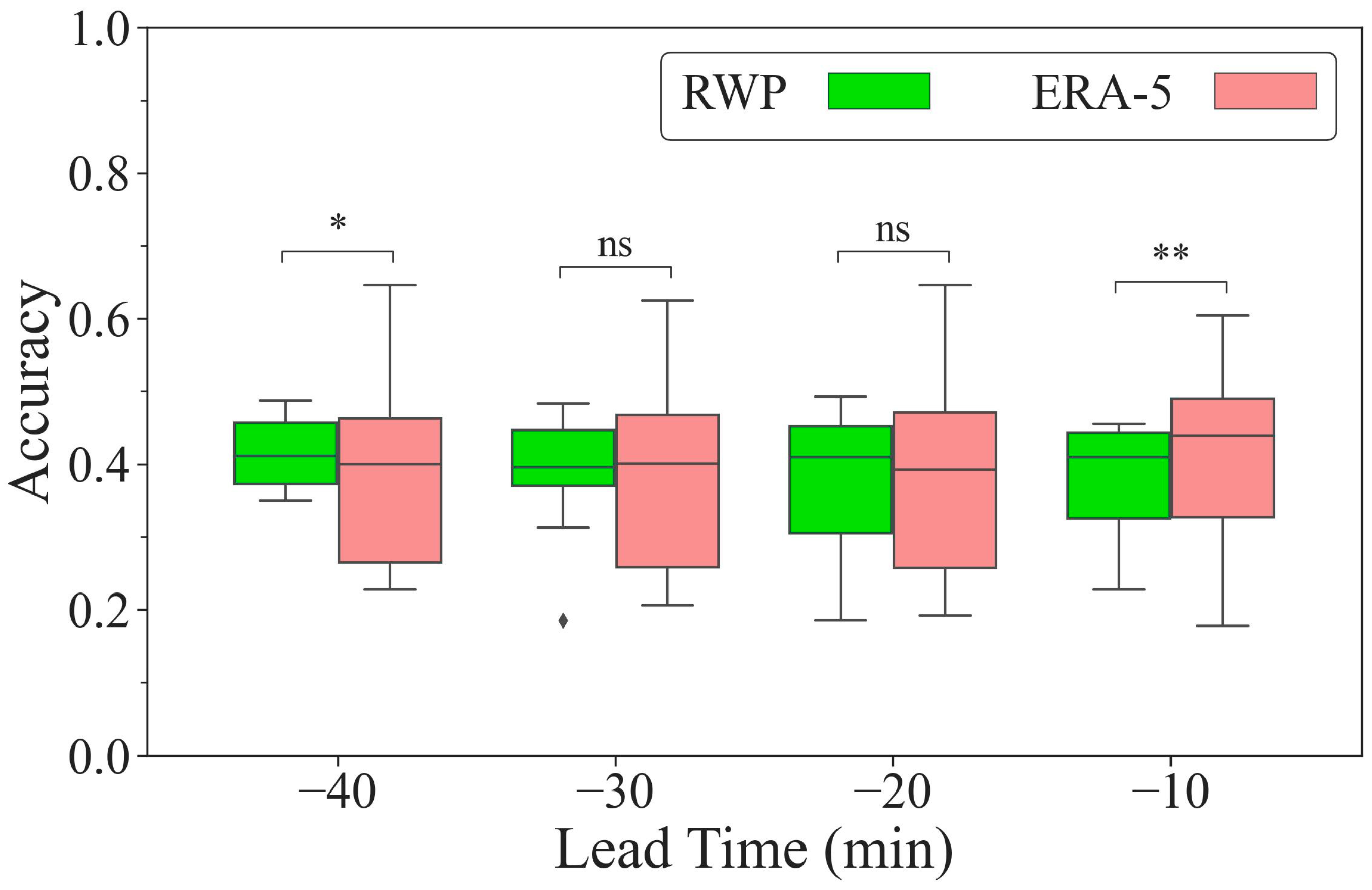
In this section, the performance of the rainfall grade forecast based on the RF model using RWP observational data (muti-class RWP model) and ERA-5 reanalysis (muti-class ERA-5 model) are evaluated. Figure 11 shows the accuracy of the muti-class RWP model and the muti-class ERA-5 model within 30 min before the onset of each rainfall process. Compared with the forecast using the muti-class ERA-5 model, the muti-class RWP model has a relatively centralized accuracy score, which becomes less obvious as the time of rainfall approaches. In particular, the muti-class ERA-5 model is superior to the muti-class RWP model in the view of accuracy at the lead time of 10 min only.

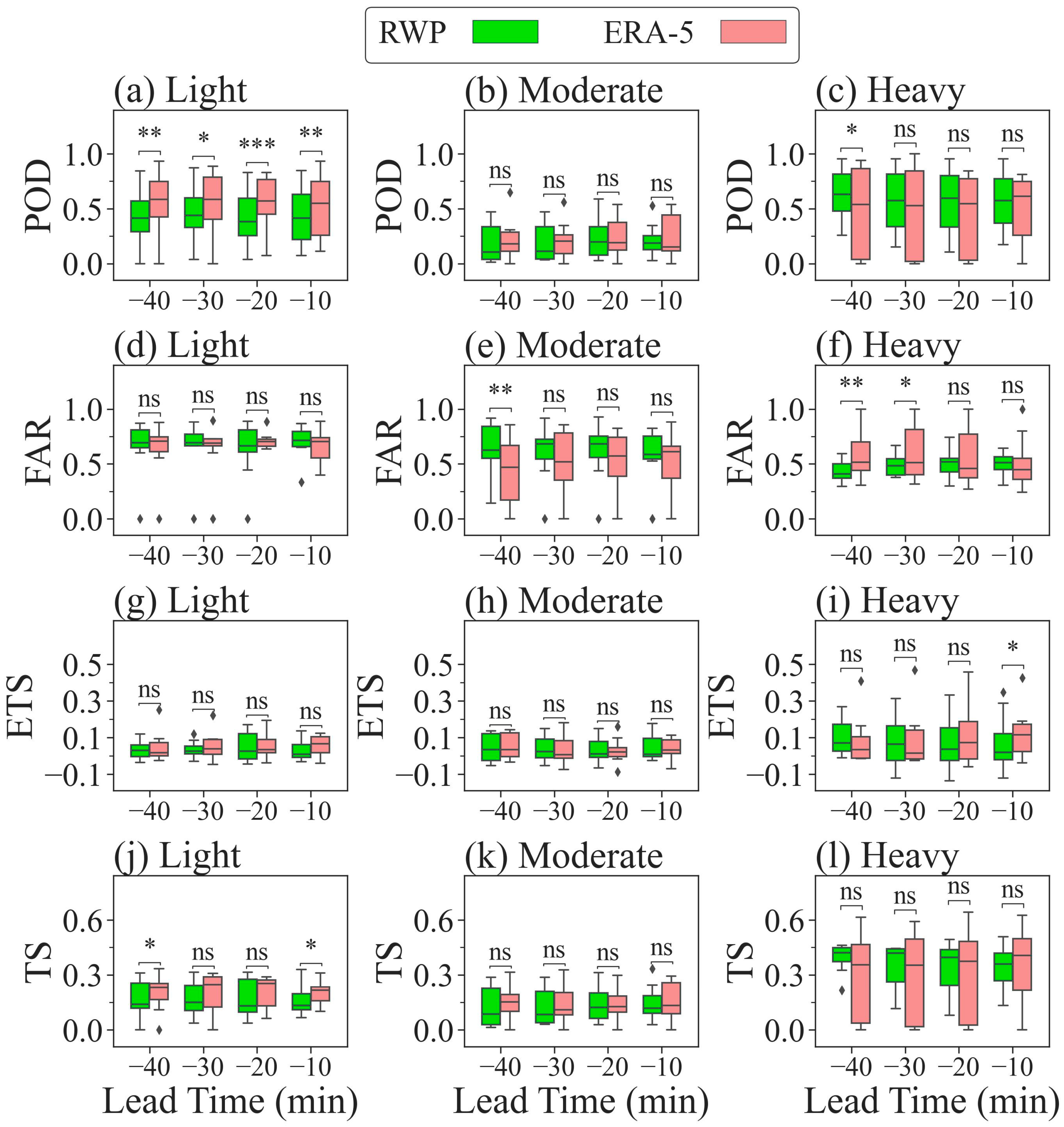
In addition, we evaluate the model performance for different rainfall grades, which is shown in Figure 12. For light rain, the POD scores for all of the forecast ranges (30, 20, and 10 min) from the muti-class RWP model are much higher compared to those from the muti-class ERA-5 model. By comparison, the multi-class ERA-5 model shows advantages in POD for its higher POD scores for all of the forecast ranges. ETS and TS do not exhibit much discrepancy for either of the models. For moderate rain, both of the models tend to provide similar forecast given that the difference does not pass the statistical significance test. For heavy rain, the muti-class RWP model produces a higher median POD score, but a much lower FAR score than the muti-class ERA-5 model in all of the forecast ranges. Interestingly, more than 75% of the heavy rainfall forecast by the muti-class RWP model has a TS score greater than 0.3. In contrast, the multi-class ERA-5 model produces a TS score approaching 0 in some cases. The FAR score from the multi-class ERA-5 model is higher at 30 and 20 min before the rainfall onset. This suggests that the muti-class RWP model produces better rainfall nowcasting skill than the multi-class ERA-5 model, especially for heavy rainfall.

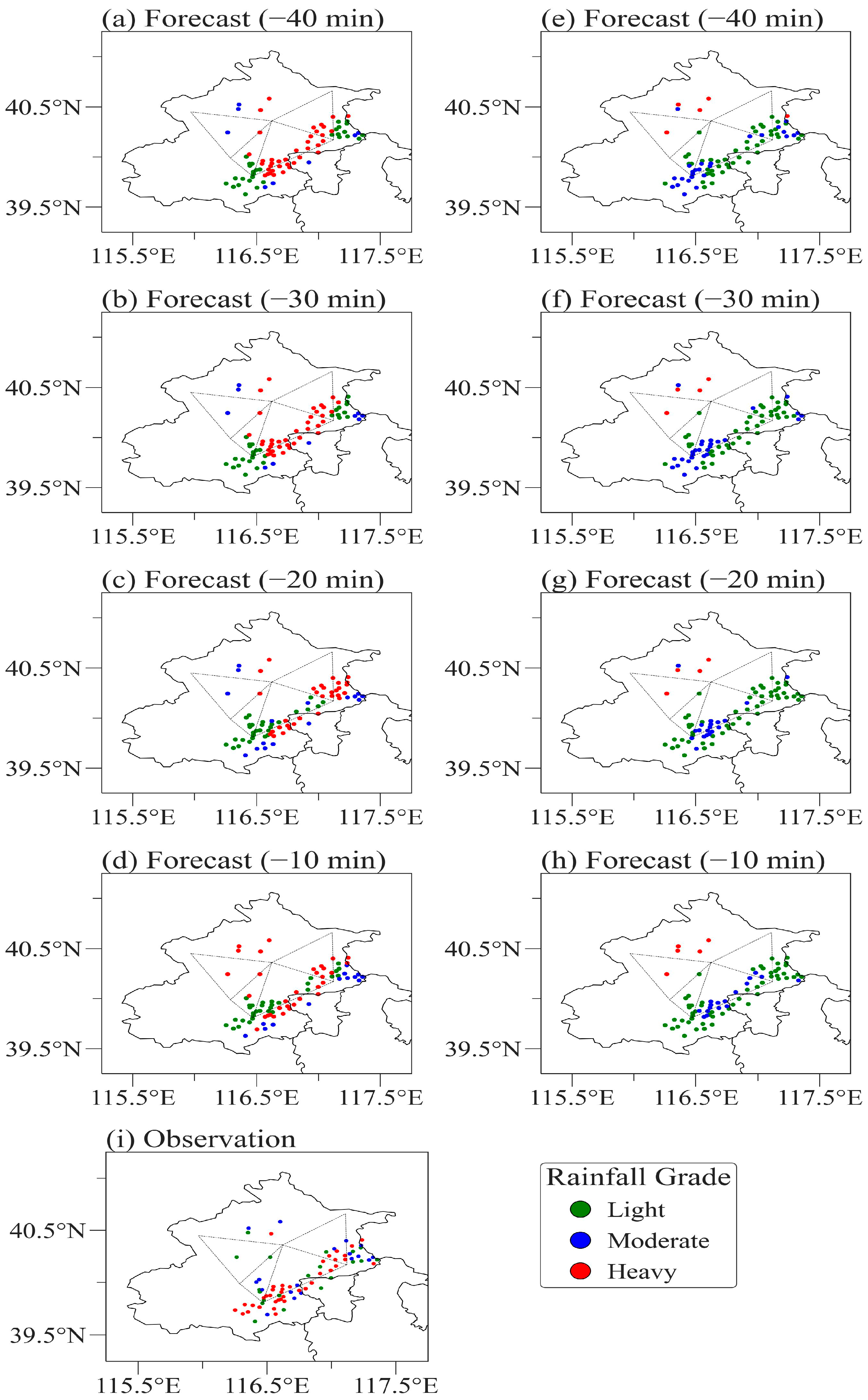
Figure 13 shows the forecast output of the muti-class RWP model and the muti-class ERA-5 model, which is the same as Figure 10 but for the grade forecast for the rainfall event initiated at 12:10 Beijing time (BJT) on 12 August 2018. The green, blue, and red dots indicate the weather stations with light, moderate, and heavy rain forecast, respectively. The muti-class RWP model can predict heavy rain in the northern and central part of the rainfall region, while the muti-class ERA-5 model may underestimate the rainfall grade. The criteria in

Table 5. The same as Table 4, but for the grade forecast of the rainfall case that occurred at 12:10 BJT on 12 August 2018.

Metrics	Grades	Lead Time (min)
		−40		−30		−20		−10
		RWP	ERA-5	RWP	ERA-5	RWP	ERA-5	RWP	ERA-5
Accuracy	All	0.49	0.25	0.46	0.22	0.32	0.26	0.33	0.24
POD	Light	0.50	0.600	0.45	0.60	0.30	0.75	0.35	0.75
	Mod.	0.17	0.28	0.17	0.22	0.22	0.22	0.17	0.11
	Heavy	0.63	0.05	0.61	0.03	0.37	0.03	0.40	0.03
FAR	Light	0.67	0.733	0.69	0.73	0.79	0.72	0.77	0.72
	Mod.	0.62	0.808	0.7	0.86	0.75	0.79	0.77	0.88
	Heavy	0.37	0.6	0.38	0.75	0.55	0.75	0.53	0.8
TS	Light	0.25	0.226	0.23	0.23	0.14	0.26	0.16	0.25
	Mod.	0.13	0.128	0.12	0.09	0.13	0.12	0.11	0.06
	Heavy	0.46	0.049	0.44	0.02	0.26	0.02	0.27	0.02
ETS	Light	0.07	0.01	0.04	0.01	−0.04	0.02	−0.03	0.02
	Mod.	0.05	−0.04	0.03	−0.07	0.01	−0.02	−0.01	−0.07
	Heavy	0.15	−0.01	0.13	−0.03	−0.04	−0.03	−0.03	−0.04

can also reflect this point. When the muti-class RWP model is used, the score of heavy rain is higher than that using the muti-class ERA-5 model; however, for light rain and moderate rain, the score when using the muti-class ERA-5 model is higher than that using the muti-class RWP model. From the overall accuracy score of each magnitude, the accuracy rate of the rainfall grade forecast model using the muti-class RWP model is still better than that using the muti-class ERA-5 model.

4. Conclusions

In this study, the divergence, vorticity, and vertical velocity features before the onset of rainfall are calculated by using the observational data of the radar wind profiler (RWP) network in Beijing. After temporal-spatial matching and interpolation, the RWP data are matched with HW-8 satellite data, ERA-5 reanalysis, and 1-min rainfall observation data (rainfall gauges), and a set of machine learning datasets is constructed by synthesizing the observation and reanalysis data.

The time-lag correlation analysis has been used here between the rainfall and atmospheric dynamic variables at various heights. The results show that the divergence, vorticity, and vertical velocity features from the RWP mesonet observation are correlated with the rainfall within 30 min before the beginning of rainfall, indicating that those features are pivotal key pre-storm signals.

Furthermore, the forecast models that are based on the random forest algorithm are developed for the rainfall/non-rainfall forecast (binary model) and the rainfall grade forecast (muti-class model). The model forecasting performance is assessed and compared for the two RF models by varying the different data sources of divergence, vorticity, and vertical velocity features. One is from the measurements of the RWP mesonet in Beijing and another from the ERA-5 reanalysis. The atmospheric dynamic variables exhibit a quite different feature importance score for both the binary RF model and the muti-class RF model, which are used to carry out the rainfall/non-rainfall forecast and the rainfall grade forecast, respectively. This indicates that the importance scores vary dramatically, depending on the data sources. When the atmospheric dynamic features such as D, ξ, and ω are estimated from RWP observations, the divergence and vorticity at 800 hPa are emphasized in the rainfall grade forecast, whereas the features of divergence, vorticity, and vertical velocity are generally less important than the thermodynamic features, and they are more concentrated and lower in the ranking for the rainfall/non-rainfall forecast. The features that are driven by satellite are considered to be the most important in both of the forecasts.

The independence dataset is used for evaluating in the binary model and the muti-class model. Further analysis is carried out for the model performance difference between both of the RF models by varying the data sources (i.e., RWP observation and ERA-5 reanalysis) for the estimated features, such as D, ξ, and ω. The RF classification model for the rainfall/non-rainfall forecast, which uses RWP data as the source of D, ξ, and ω features, has a better effect than the model that is based on ERA-5 reanalysis. In addition, for the rainfall grade forecast, the RF classification model using the RWP-derived D, ξ, and ω features tends to produce a much more reasonable spatial pattern of moderate rain and heavy rainfall forecast.

In a word, the usage of dynamic variables from the RWP mesonet measurements improves the prediction skill of rainfall to some degree. Nevertheless, there exist no valid measured profiles of thermodynamic variables. This will inevitably impair our understanding of the pre-storm environment. In the future, the profiles will become available for temperature and humidity, particularly below the cloud base, from the microwave radiometer observational network, along with the geostationary satellite. These observations are hopefully beneficial for the prediction skill of rainfall. Last but not least, the advanced machine learning methods are warranted to be applied in order to address the weakness or shortcomings of the random forest algorithm that has been used in the present study.

References

- Ravuri, S.; Lenc, K.; Willson, M.; Kangin, D.; Lam, R.; Mirowski, R.; Fitzsimons, M.; Athanassiadou, M.; Kashem, S.; Madge, S.; et al. Skilful precipitation nowcasting using deep generative models of radar. Nature 2021, 597, 672–677. [Google Scholar] [CrossRef] [PubMed]
- Jonassen, M.O.; Ólafsson, H.; Ágústsson, H.; Rögnvaldsson, Ó.; Reuder, J. Improving High-Resolution Numerical Weather Simulations by Assimilating Data from an Unmanned Aerial System. Mon. Weather Rev. 2012, 140, 3734–3756. [Google Scholar] [CrossRef] [Green Version]
- Li, Z. Impact of assimilating Mode-S EHS winds in the Met Office’s high-resolution NWP model. Meteorol. Appl. 2021, 28, e1989. [Google Scholar] [CrossRef]
- Mueller, C.K.; Saxen, T.; Roberts, R.; Wilson, J.; Betancourt, T.; Dettling, S.; Oien, N.; Yee, J. NCAR Auto-Nowcast System. Weather Forecast. 2003, 18, 545–561. [Google Scholar] [CrossRef]
- Wilson, J.W.; Feng, Y.R.; Chen, M.; Roberts, R.D. Nowcasting challenges during the Beijing Olympics: Successes, failures, and implications for future nowcasting systems. Weather Forecast. 2010, 25, 1691–1714. [Google Scholar] [CrossRef]
- Ballard, S.; Li, Z.; Davud, S.; Helen, B.; Cristina, C.P.; Nicolas, G.; Lee, H.S. Use of radar data in NWP-based nowcasting in the Met Office. In Proceedings of the Weather Radar and Hydrology Symposium, Exeter, UK, 18 April 2011. [Google Scholar]
- Pulkkinen, S.; Chandrasekar, V.; Lerber, A.V.; Harri, A.M. Nowcasting of Convective Rainfall Using Volumetric Radar Observations. IEEE Trans. Geosci. Remote Sens. 2020, 58, 7845–7859. [Google Scholar] [CrossRef]
- Mecikalski, J.R.; Li, X.L.; Carey, L.D.; McCaul, E.W.; Coleman, T.A. Regional comparison of GOES cloud-top properties and radar characteristics in advance of first-flash lightning initiation. Mon. Weather Rev. 2013, 141, 55–74. [Google Scholar] [CrossRef] [Green Version]
- Bedka, M.; Wang, C.; Rogers, R.; Carey, L.D.; Feltz, W.; Kanak, J. Examining deep convective cloud evolution using total lightning, WSR-88D, and GOES-14 super rapid scan datasets. Weather Forecast. 2015, 30, 571–590. [Google Scholar] [CrossRef]
- Gravelle, C.M.; Mecikalski, J.R.; Line, W.E.; Bedka, K.M.; Petersen, R.A.; Sieglaff, J.M.; Stano, G.T.; Goodman, S.J. Demonstration of a GOES-R satellite convective toolkit to “bridge the gap” between severe weather watches and warnings: An example from the 20 May 2013 Moore, Oklahoma, tornado outbreak. Bull. Am. Meteorol. Soc. 2016, 97, 69–84. [Google Scholar] [CrossRef]
- Baker, N.L.; Daley, R. Observation and background adjoint sensitivity in the adaptive observation-targeting problem. Quart. J. R. Meteorol. Soc. 2000, 126, 1431–1454. [Google Scholar] [CrossRef]
- Majumdar, S.J. A Review of Targeted Observations. Bull. Am. Meteorol. Soc. 2016, 97, 2287–2303. [Google Scholar] [CrossRef]
- Chiara, G.D.; Bonavita, M.; English, S.J. Improving the Assimilation of Scatterometer Wind Observations in Global NWP. IEEE J. Sel. Top. Appl. Earth Obs. Remote Sens. 2017, 10, 2415–2423. [Google Scholar] [CrossRef]
- Janisková, M.; Fielding, M.D. Direct 4D-Var assimilation of space-borne cloud radar and lidar observations. Part II: Impact on analysis and subsequent forecast. Q. J. R. Meteorol. Soc. 2020, 146, 3877–3899. [Google Scholar] [CrossRef]
- Caumont, O.; Cimini, D.; Löhnert, U.; Lucas, A.A.; Bleisch, R.; Buffa, F.; Ferrario, M.E.; Haefele, A.; Huet, T.; Madonna, F.; et al. Assimilation of humidity and temperature observations retrieved from ground-based microwave radiometers into a convective-scale NWP model. Q. J. R. Meteorol. Soc. 2016, 142, 2692–2704. [Google Scholar] [CrossRef] [Green Version]
- Wang, C.; Chen, M.; Chen, Y. Impact of Combined Assimilation of Wind Profiler and Doppler Radar Data on a Convective-Scale Cycling Forecasting System. Mon. Weather Rev. 2022, 150, 431–450. [Google Scholar] [CrossRef]
- Wang, D.; Giangrande, S.E.; Feng, Z.; Hardin, J.C.; Prein, A.F. Updraft and Downdraft Core Size and Intensity as Revealed by Radar Wind Profilers: MCS Observations and Idealized Model Comparisons. J. Geophys. Res. Atmos. 2020, 125, e2019JD031774. [Google Scholar] [CrossRef]
- Zhang, Y.; Gou, J.; Yang, Y.J.; Wang, Y.; Yim, S. Vertical Wind Shear Modulates Particulate Matter Pollutions: A Perspective from Radar Wind Profiler Observations in Beijing, China. Remote Sens. 2020, 12, 546. [Google Scholar] [CrossRef] [Green Version]
- Giangrande, S.E.; Biscaro, T.; Peters, J.M. Seasonal Controls on Isolated Convective Storm Drafts, Precipitation Intensity, and Life Cycle as Observed During GoAmazon2014/5. EGUsphere, 2022; manuscript in preparation. [Google Scholar]
- Liu, B.; Gou, J.; Gong, W.; Zhang, Y.; Ma, Y. Characteristics and performance of wind profiles as observed by the radar wind profiler network of China. Atmos. Meas. Tech. 2020, 13, 4589–4600. [Google Scholar] [CrossRef]
- Guo, X.; Guo, J.; Zhang, D.L.; Yun, Y. Vertical Divergence Profiles as Detected by a Wind Profiler Mesonet over East China: Implications for Nowcasting Convective Storms. Q. J. 2023; manuscript in preparation. [Google Scholar]
- Akdi, Y.; Ünlü, K.D. Periodicity in precipitation and temperature for monthly data of Turkey. Theor. Appl. Climatol. 2021, 143, 957–968. [Google Scholar] [CrossRef]
- Han, L.; Sun, J.; Zhang, W. Convolutional Neural Network for Convective Storm Nowcasting Using 3-D Doppler Weather Radar Data. IEEE Trans. Geosci. Remote Sens. 2019, 58, 1487–1495. [Google Scholar] [CrossRef]
- Han, L.; Zhao, Y.; Chen, H.; Chandrasekar, V. Advancing Radar Nowcasting Through Deep Transfer Learning. IEEE Trans. Geosci. Remote Sens. 2021, 60, 4100609. [Google Scholar] [CrossRef]
- Mecikalski, J.R.; Williams, J.K.; Jewett, C.P.; Ahijevych, D.; LeRoy, A.; Walker, J.R. Probabilistic 0–1-h convective initiation nowcasts that combine geostationary satellite observations and numerical weather prediction model data. J. Appl. Meteorol. Climatol. 2015, 54, 1039–1059. [Google Scholar] [CrossRef] [Green Version]
- Gao, H.; Shen, C.; Zhou, Y.; Wang, X.; Chan, P.; Hon, K.; Zhou, D.; Li, J. A Spatio-Temporal Neural Network for Fine-Scale Wind Field Nowcasting Based on Lidar Observation. IEEE J. Sel. Top. Appl. Earth Obs. Remote Sens. 2022, 15, 5596–5606. [Google Scholar] [CrossRef]
- Han, L.; Sun, J.; Zhang, W.; Xiu, Y.; Feng, H.; Lin, Y. A machine learning nowcasting method based on real-time reanalysis data. J. Geophys. Res. Atmos. 2017, 122, 4038–4051. [Google Scholar] [CrossRef] [Green Version]
- Zhou, K.; Zheng, Y.; Li, B.; Dong, W.; Zhang, X. Forecasting Different Types of Convective Weather: A Deep Learning Approach. J. Meteorol. Res. 2019, 33, 797–809. [Google Scholar] [CrossRef]
- Zhou, K.; Sun, J.; Zheng, Y.; Zhang, Y. Quantitative Precipitation Forecast Experiment Based on Basic NWP Variables Using Deep Learning. Adv. Atmos. Sci. 2020, 39, 1472–1486. [Google Scholar] [CrossRef]
- Ahijevych, D.; Pinto, J.; Willliams, J.K.; Steiner, M. Probabilistic forecasts of mesoscale convective system initiation using the random forest data mining technique. Weather Forecast. 2016, 31, 581–599. [Google Scholar] [CrossRef]
- Leinonen, J.; Hamann, U.; Germann, U.; Mecikalski, J.R. Nowcasting thunderstorm hazards using machine learning: The impact of data sources on performance. Nat. Hazards Earth Syst. Sci. 2021, 22, 577–597. [Google Scholar] [CrossRef]
- Liu, X.; Chen, H.; Han, L.; Ge, Y. A Machine Learning Approach for Convective Initiation Detection Using Multi-Source Data. In Proceedings of the IGARSS 2022—2022 IEEE International Geoscience and Remote Sensing Symposium, Kuala Lumpur, Malaysia, 17–22 July 2022. [Google Scholar]
- Breiman, L. Random forests. Mach. Learn. 2001, 45, 5–32. [Google Scholar] [CrossRef] [Green Version]
- Hill, A.J.; Schumacher, R.S.; Jirak, I.L. A New Paradigm for Medium-range Severe Weather Forecasts: Probabilistic Random Forest-based Predictions. Weather Forecast. 2022, 38, 251–272. [Google Scholar] [CrossRef]
- McCandless, T.; Gagne, D.; Kosović, B.; Haupt, S.E.; Yang, B.; Becker, C.; Schreck, J. Machine Learning for Improving Surface-Layer-Flux Estimates. Bound. Layer Meteorol. 2021, 185, 199–228. [Google Scholar] [CrossRef]
- Bellamy, J.C. Objective calculations of divergence, vertical velocity and vorticity. Bull. Am. Meteorol. Soc. 1949, 30, 45–49. [Google Scholar] [CrossRef]
- Bessho, K.; Date, K.; Hayashi, M.; Ikeda, A.; Imai, T.; Inoue, H.; Kumagai, Y.; Miyakawa, T.; Murata, H.; Ohno, T.; et al. An introduction to Himawari-8/9-Japan’s new generation geostationary meteorological satellites. J. Meteorol. Soc. Jpn. 2016, 94, 151–183. [Google Scholar] [CrossRef] [Green Version]
- Mecikalski, J.R.; Bedka, K.M. Forecasting Convective Initiation by Monitoring the Evolution of Moving Cumulus in Daytime GOES Imagery. Mon. Weather Rev. 2006, 134, 49–78. [Google Scholar] [CrossRef] [Green Version]
- Chen, D.; Guo, J.; Yao, D.; Lin, Y.; Zhao, C.; Min, M.; Xu, H.; Liu, L.; Huang, X.; Chen, T.; et al. Mesoscale convective systems in the Asian monsoon region from advanced Himawari imager: Algorithms and preliminary results. J. Geophys. Res. Atmos. 2019, 124, 2210–2234. [Google Scholar] [CrossRef] [Green Version]
- Chen, D.; Guo, J.; Yao, D.; Feng, Z.; Lin, Y. Elucidating the life cycle of warm-season mesoscale convective systems in eastern China from the Himawari-8 geostationary satellite. Remote Sens. 2020, 12, 2307. [Google Scholar] [CrossRef]
- Hoffmann, L.; Günther, G.; Li, D.; Stein, O.; Wu, X.; Griessbach, S.; Heng, Y.; Konopka, P.; Müller, R.; Vogel, B.; et al. From ERA-Interim to ERA5: The considerable impact of ECMWF’s next-generation reanalysis on Lagrangian transport simulations. Atmos. Chem. Phys. 2019, 19, 3097–3124. [Google Scholar] [CrossRef] [Green Version]
- Altman, N.; Krzywinski, M. Ensemble methods: Bagging and random forests. Nat. Methods 2017, 14, 933–935. [Google Scholar] [CrossRef]
- Chen, Z.Y.; Zhang, T.H.; Zhang, R.; Zhu, Z.M.; Yang, J.; Chen, P.Y.; Ou, C.Q.; Guo, Y. Extreme gradient boosting model to estimate PM 2.5 concentrations with missing-filled satellite data in China. Atmos. Environ. 2019, 202, 180–189. [Google Scholar] [CrossRef]
- Di, Q.; Amin, H.; Shi, L.; Kloog, I.; Silvern, R.; Kelly, J.; Sabath, M.B.; Choirat, C.; Koutrakis, P.; Lyapustin, A.; et al. An ensemble-based model of PM2.5 concentration across the contiguous United States with high spatiotemporal resolution. Environ. Int. 2019, 130, 104909. [Google Scholar] [CrossRef] [PubMed]
- Genuer, R.; Poggi, J.M.; Christine, T.M. Variable selection using random forests. Pattern Recognit. Lett. 2010, 31, 2225–2236. [Google Scholar] [CrossRef] [Green Version]
Figure 1.
Spatial distribution map of rain gauge stations, radar wind profiler (RWP) stations, Himawari-8 (HW-8) satellite pixels, and ERA-5 reanalysis grids in the study area. (a) is the spatial distribution diagram of rain gauge stations and RWP stations in the study area, where blue dots represent rain gauge stations, orange dots represent RWP stations, black dotted lines represent triangular boundaries formed by three RWP stations, and the solid square grid represents an ERA-5 grid with the weight of RWP observational data (described in Section 2.3) greater than or equal to 10%. (b) is the spatial matching diagram of the triangle network of the RWP and ERA-5 grid, where the black solid line represents the boundary of the ERA-5 grid and the color-shaded parts represent the overlapping parts of the triangle composed of different RWP and the ERA-5 grid. (c) is the spatial matching diagram of the rain gauge station (solid blue dot) and Himawari-8 (HW-8) satellite pixel (blue box).
Figure 2.
The observed rainfall probability distribution of all rain gauges in the study area during the summer of 2018–2019, in which the green line represents the 33.33% quantile and the red line represents the 66.66% quantile. The above figure is the box chart of rainfall intensity, with the 25th, 50th, and 75th percentiles represented from left to right. While the outside of the box extends to 1.5 times the quartile deviation (25th to 75th percentile), the outliers are indicated by black dots.
Figure 3.
Flow chart of random forest model establishment and training.
Figure 4.
Time-lag correlation coefficients between rainfall intensity and (a) divergence, (b) vertical velocity, and (c) vorticity (at 10-min intervals) retrieved from the RWP mesonet within 30 min before the onset of rainfall (−42–−12 min). The black solid grid points represent statistical significance passing the 99% confidence level.
Figure 5.
Scatter plots between rainfall amount at t = 0–10 min (a) divergence, (b) vertical velocity, and (c) vorticity retrieved from the RWP mesonet within 30 min before the onset of rainfall (−42–−12 min). The regression lines are also shown.
Figure 6.
The OOB (out-of-bag) score of the random forest classification model used for rainfall/non-rainfall forecast (binary class, blue) and rainfall grade forecast (muti-class, red) changes along with the removal of undetermined features. T the corresponding feature removal sequence of each model is shown in Table 2.
Figure 7.
The same as Figure 5 but for the OOB score as a function of the number of decision trees (DT).
Figure 8.
The feature importance score of the RF classification model for the rainfall/non-rainfall forecast (a,b) and rainfall grade forecast (c,d), which are based on the feature variables of D, ξ, and ω from different data sources ((a,c) are from RWP and (b,d) are from ERA-5).
Figure 9.
The performance of the RF classification model for rainfall/non-rainfall forecast within 30 min before the onset of rainfall, where the input features of D, ξ, and ω are from the RWP (in green) and ERA-5 (in pink), respectively. The evaluation metrics include POD (a), FAR (b), accuracy (c), AUC (d), TS (e), and ETS (f). * and ** above the box plot represents statistical significance passing the 95% and 99% confidence level, whereas “ns” represents no statistical significance, and outliers are indicated by black dots.
Figure 10.
The forecast output results of the random forest model within 30 min before the rainfall initiated at 23:20 BJT on 16 July 2018, where panels (a–d) are based on the features of divergence, vorticity, and vertical velocity from the RWP measurements (the binary RWP model) and panels (e–h) are from the ERA-5 reanalysis data (the binary ERA-5 model). The panels (i) is the rainfall observation record at 23:20 BJT.
Figure 11.
Box plots showing the accuracy used to assess the RF model for the rainfall grade forecast, which is based on RWP measurements (in green) and ERA-5 reanalysis data (in pink), respectively. * and ** above the box plot represents statistical significance passing the 95% and 99% confidence level, whereas “ns” represents no statistical significance, and outliers are indicated by black dots.
Figure 12.
The same as Figure 9 but for the results of the rainfall grade forecast. * and ** above the box plot represents statistical significance passing the 95% and 99% confidence level, whereas “ns” represents no statistical significance, and outliers are indicated by black dots.
Figure 13.
The same as Figure 10 but for the grade forecast of the rainfall initiated at 12:10 BJT on 12 August 2018, where panels (a–d) are based on the features of divergence, vorticity, and vertical velocity from the RWP measurements (the binary RWP model) and panels (e–h) are from the ERA-5 reanalysis data (the binary ERA-5 model). The panels (i) is the rainfall observation record at 12:10 BJT. The green, blue, and red dots represent the rain gauge stations with light, moderate, and heavy rain forecast, respectively.