


Rapid Mapping of Slow-Moving Landslides Using an Automated SAR Processing Platform (HyP3) and Stacking-InSAR Method

1
National Institute of Natural Hazards, Ministry of Emergency Management of China, Beijing 100085, China
2
School of Earth Sciences and Resources, China University of Geosciences (Beijing), Beijing 100083, China
3
Faculty of Geomatics, East China University of Technology, Nanchang 330013, China
*
Author to whom correspondence should be addressed.
Remote Sens. 2023, 15(6), 1611; https://doi.org/10.3390/rs15061611
Submission received: 13 January 2023
/
Revised: 17 February 2023
/
Accepted: 14 March 2023
/
Published: 16 March 2023
(This article belongs to the Special Issue Landslide Inventory Mapping and Monitoring Using Remote Sensing Techniques)
Abstract
:The increasing number of landslide hazards worldwide has placed greater demands on the production and updating of landslide inventory maps. As an important data source for landslide detection, interferometric synthetic aperture radar (InSAR) data processing is time-consuming and also requires specialized knowledge, which severely hinders its widespread application. At present, a new cloud-based online platform, i.e., Alaska Satellite Facility’s Hybrid Pluggable Processing Pipeline (ASF HyP3) was developed for massive SAR data processing. In this study, combining the HyP3 online platform and Stacking-InSAR method, we constructed a new easy-to-use processing chain for rapidly identifying slow-moving landslides over large areas. With this processing chain, a total of 923 interferometric pairs covering an area of over 1800 km2 were processed within a few hours (about 4 to 5 h). A total of 81 slow-moving landslides were immediately detected and mapped using Stacking-InSAR method, of which 65 landslides were confirmed by previous studies and 16 landslides were newly detected. Results show that the new processing chain can greatly improve the efficiency of wide-area landslide mapping and is expected to serve as an effective tool for rapid updating the existing landslide inventories and contribute to the prevention and management of geological hazards.
1. Introduction
Landslides are a common geological phenomenon in mountainous areas, and they can lead to significant death and property damage [1,2]. In China, recent catastrophic landslides such as the 24 June 2017 Xinmo landslide [3], the October and November 2018 Baige landslide [4], are characterized by high altitude, hidden locations, long dormant periods and rapid movement, making it difficult to identify such disasters during on-site investigations [5]. Moreover, in the context of global climate change and human activity, landslide hazards will become more frequent [6,7]. Thus, developing a rapid landslide mapping method over large areas is an urgent need for disaster prevention and mitigation.
Slow-moving landslides usually occur in areas with mechanically weak soil/rock and high seasonal rainfall [8], with a slow rate of material movement (mm/year to m/year) [9]. Usually, slow-moving landslides are difficult to identify due to the imperceptible deformation and dense vegetation cover. The synthetic aperture radar (SAR) data has the advantage of wide coverage (about 250 km for Sentinel-1 image) and penetrating clouds/fog. On this basis, the advanced Interferometric SAR (InSAR) technologies such as differential InSAR (D-InSAR) [10], persistent scatterer InSAR (PS-InSAR) [11], and small baseline subset InSAR (SBAS-InSAR) [12,13,14] are very suitable for measuring subtle surface displacements [15,16,17], which have great potential for identifying these slow-moving landslides [18,19,20,21]. For instance, ref. [22] adopted the time-series InSAR method to detect slow-moving landslides in the steep mountainous areas of Nepal, demonstrating the potential of the Sentinel-1 data to map landslides. Ref. [23] adopted Stacking-InSAR method to identify potential landslides in mountainous areas and proved its effectiveness by comparing it with the SBAS-InSAR method. Ref. [24] successfully interpreted 904 active landslides in an area of 179,000 km2 on the Tibetan Plateau using a combination of InSAR observations and optical images. Ref. [25] investigated slow-moving shallow soil landslides in the New Zealand region using SBAS-InSAR method. Ref. [26] analyzed the efficiency of PS-InSAR method in landslide mapping. Ref. [27] adopted the parallel SBAS technique and spatial clustering to map potential instability phenomena affecting the Italian Peninsula.
Although InSAR technology has substantial advantages in identifying slow-moving landslides, the high hardware/software requirements, time-consuming processing, and the involvement of specialized knowledge greatly limit its widespread application [28], especially the rapid mapping and updating of the existing landslide inventories. To alleviate this issue, some organizations and institutions provide freely accessible InSAR products (such as LiCSAR [29]) or cloud-based online services (such as Hybrid Pluggable Processing Pipeline (HyP3) [30]). Among them, LiCSAR products are easy to use, and with the LiCSBAS time series analysis package, users can quickly obtain large-scale deformation data with relatively reliable accuracy [29]. However, LiCSAR products with 100 m spatial resolution are more suitable for large-scale tectonic strain mapping [31]. Additionally, LiCSAR products have no available data in some regions and are less customizable. In contrast, the HyP3 is a new free cloud-based online service platform for Sentinel-1 SAR data processing, developed by NASA’s Alaska Satellite Facility Distributed Active Archive Center (ASF DAAC) [32]. It supports users to process Sentinel-1 data on demands. By submitting the jobs online, users can quickly obtain the processed products (such as wrapped/unwrapped differential interferograms). It does not require users to download and process the raw SAR data, which greatly saves storage resources, shortens the data processing time, and simplifies the InSAR data processing. However, the application of this online platform is still relatively rare [32,33], while few studies have confirmed its efficiency in landslide mapping.
In this paper, we combined the HyP3 platform and Stacking-InSAR method to construct a new easy-to-use processing chain for rapidly identifying slow-moving landslides over large areas. This processing chain has three main advantages: ease of use, small space occupation, and fast processing speed. To prove its effectiveness, the Batang section of Jinsha River, covering an area of approximately 1832 km2, was selected as the study area, where landslide disasters are very frequent. Slow-moving landslides in the study area were identified and analyzed by using this new processing chain. We expected it to be an effective tool to quickly update the existing landslide inventories and assist in the prevention and management of geological hazards.
This paper is organized as follows: Section 2 mainly describes the landslide mapping chain used in this study, Section 3 focuses on the description of the study area and the use of data, Section 4 presents the results and validation, and Section 5 discusses the results, ending with a conclusion in Section 6.
2. Methodology
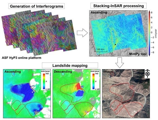
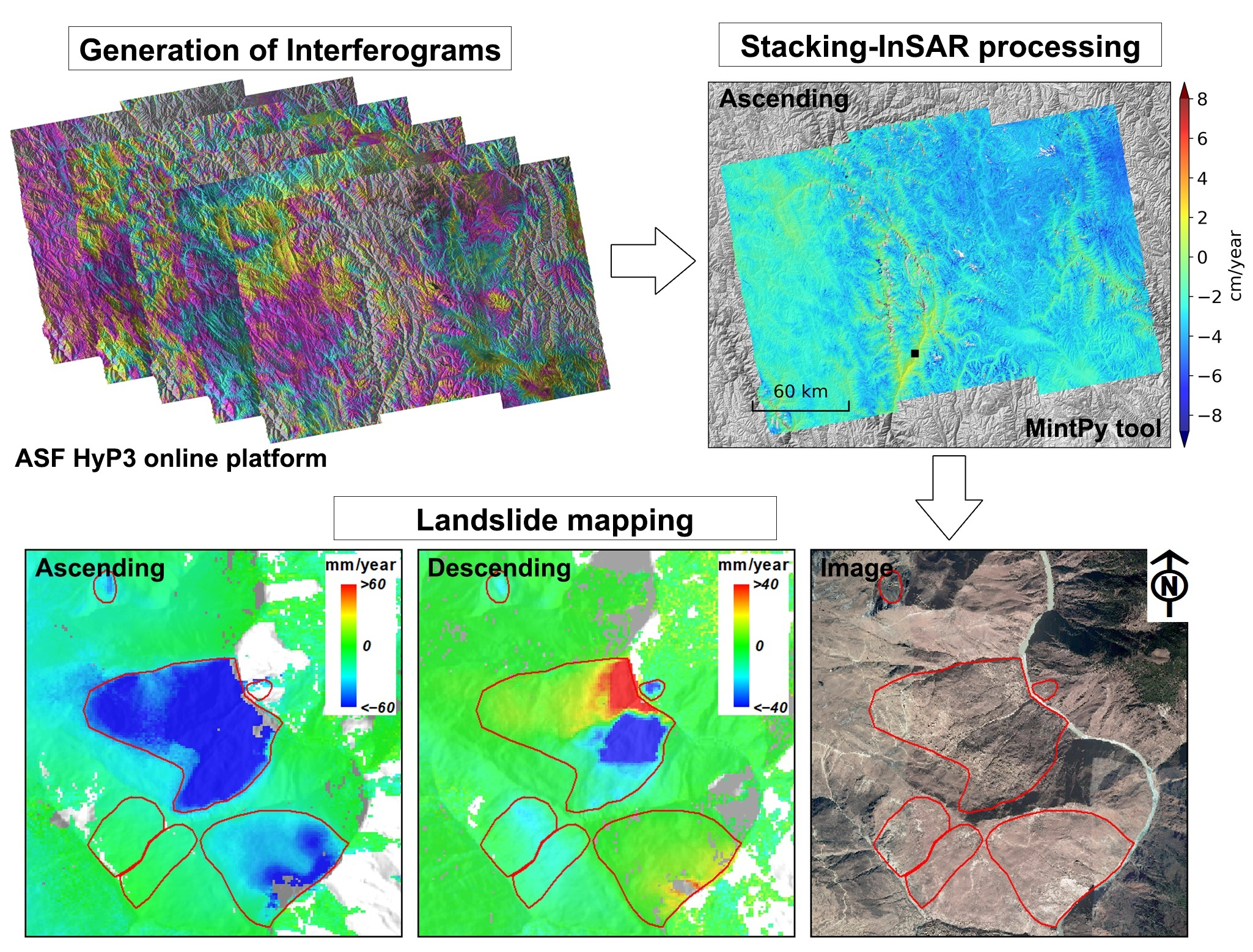
Figure 1 presents the new landslide mapping chain. It mainly includes two steps. First, Sentinel-1 SAR images of the study area were selected to generate unwrapped differential interferograms by using the HyP3 online platform. Subsequently, the Stacking-InSAR method was adopted to process these interferograms and obtain the annual deformation rate maps of the study area. Finally, slow-moving landslides were visually identified by combining optical images and digital elevation model (DEM). The open-source MintPy tool [34] was applied for Stacking-InSAR processing, meaning that the entire processing chain was open source and free to use.
2.1. Generation of Interferograms Using HyP3 Platform
The HyP3 was originally developed to solve the problems of large storage resource, time-consuming computation, and high requirements for users’ knowledge in the process of SAR data processing [30]. It is an automated SAR data processing online platform that mainly relies on core Amazon services, such as Amazon Elastic Compute Cloud and Amazon Simple Storage Service. It provides users with customized on-demand SAR processing services [32], and users are not required to purchase or install complex SAR processing software and have sophisticated SAR processing skills.
The HyP3 is primarily used to process Sentinel-1 data freely provided by European Space Agency (ESA). Based on ASF data platform, users can search and query the archived Sentinel-1 SAR data. The HyP3 can automatically access and process these archived data. Currently, the HyP3 mainly supports radiometric terrain correction (RTC), autonomous Repeat Image Feature Tracking (autoRIFT), and InSAR processing chains, all based on GAMMA software [32].
For the InSAR processing, differential interferometry is the primary type of interferometry performed by the HyP3 online platform. There are several parameters that can be set, including the temporal baseline, perpendicular baseline, and the number of looks. The temporal baseline is defined as the time interval between imaging passes. Currently, HyP3 supports a temporal baseline setting of up to 60 days. This is typically sufficient to detect geological hazards. The perpendicular baseline is the perpendicular component of the physical distance between the two acquisitions. This value should be very small to ensure coherence, and values from 0 to 300 m can be set in the HyP3. The number of looks determines the pixel spacing and the resolution of output products. The 10 × 2 looks with a 40 m pixel spacing (80 m resolution) and 20 × 4 looks with an 80 m pixel spacing (160 m resolution) can be selected by users, and the default is 20 × 4 looks with a smaller product size. In addition, users can also choose the output products, including wrapped phase, displacement maps (unwrapped), DEM, etc. A water mask can also be set during the phase unwrapping. It should be noted that the current version of the HyP3 platform only supports processing Sentinel-1 images with the VV polarization. Products are distributed as the UTM-projected GeoTIFFs format, which is convenient for subsequent analysis using relevant software.
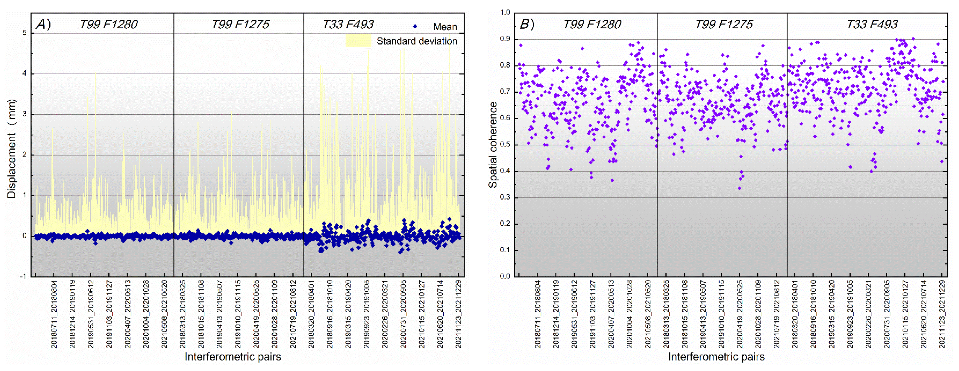
After downloading the processed products, a key step is to check the quality of the data to ensure its reliability. It consists of two main parts: one is to check the completeness of the data, and the other is to estimate the data error. Since the HyP3 platform is automated, there is a possibility that the processed products may be incomplete or even missing. In this case, a required step is to manually check the generated interferograms one by one and reprocess the incomplete ones. In addition, estimating the error of interferograms is also required, as it is difficult to guarantee that each interferogram is reliable. In this case, estimating the mean and standard deviation and calculating the spatial coherence of these interferograms are critical for selecting high quality interferograms. Finally, the cropping of data according to the extent of the study area should be considered to further decrease the computational expense.
2.2. Landslide Mapping Using Stacking-InSAR Method
The Stacking-InSAR method was first proposed by [35]. It is an enhancement technique that obtains the average deformation rate by linearly stacking a set of unwrapped differential interferograms [36]. The assumption behind this method is that in independent differential interferograms, the atmospheric error phase is random and equal, and the deformation rate over the region is approximately linear. Based on this assumption, the Stacking-InSAR method can effectively reduce the impact of atmospheric delay and obtain the accurate average deformation rate [36]. Here, the Stacking-InSAR method adopts the temporal baseline to weight the data. The average velocity is estimated by the following equation.
where Vdef represents the average velocity after stacking, phi represents the unwrapped phase, ∆t represents the temporal baseline of the differential interferogram, and n represents the number of differential interferograms to be stacked. In this study, we aimed to achieve fast landslide detection. Thus, we did not apply any additional processing, such as atmospheric correction, when performing the Stacking-InSAR processing.
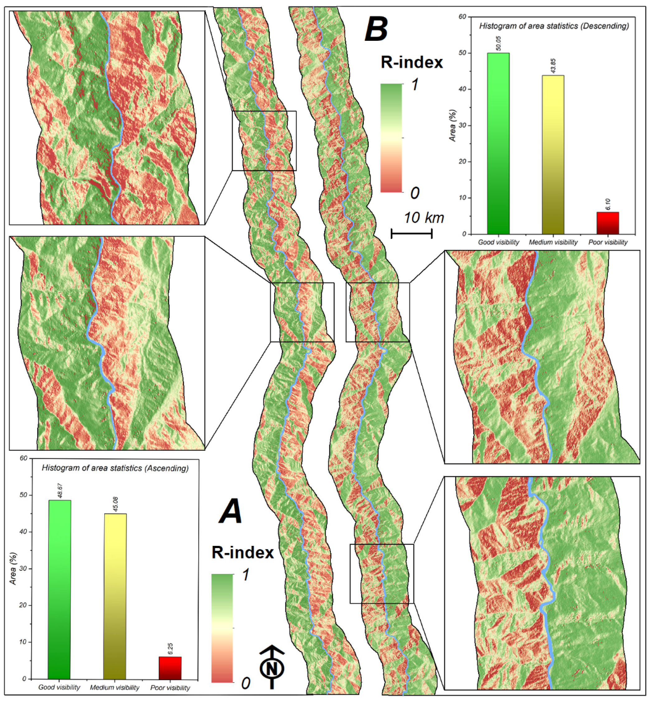
Due to the limitations of SAR satellite side-view imaging and terrain conditions, it is necessary to analyze the visibility of SAR satellites prior to landslide mapping. According to the geometric relationship between satellite orientation and local terrain, there are three main types of geometric distortions, i.e., foreshortening, layover, and shadow. Among them, the layover and shadow areas in the SAR images have poor visibility and deformation in these areas cannot be effectively detected by InSAR techniques [37,38]. In this study, R-index was applied to measure the effect of topography on SAR images [38]. The R-index denotes the ratio between the slant range and the ground range and can be calculated from satellite geometry parameters and DEM data. The calculation equation is as follows:
where S represents the local terrain slope, A represents the aspect, θ represents the azimuth angle of SAR satellite, α represents the incident angle of SAR satellite, Sh represents the shadow coefficient, and La represents the layover coefficient. The values of Sh and La can be calculated by the GIS-based shadow model. The detailed calculation steps can be found in [38]. The value of the R-index varies between 0 and 1, with a value of 0 indicating poor visibility (layover and shadow). The value between 0 and sin(α) indicates medium visibility (foreshortening), and greater than sin(α) indicates good visibility. In this study, the layover and shadow areas were masked to avoid misidentification.
Finally, slow-moving landslides in the study area were visually identified by using the average deformation rate maps. The optical images and DEM data were also used to refine landslide boundaries. The identification results were validated by comparing them one by one with the existing landslide inventories.
3. Study Area and Data
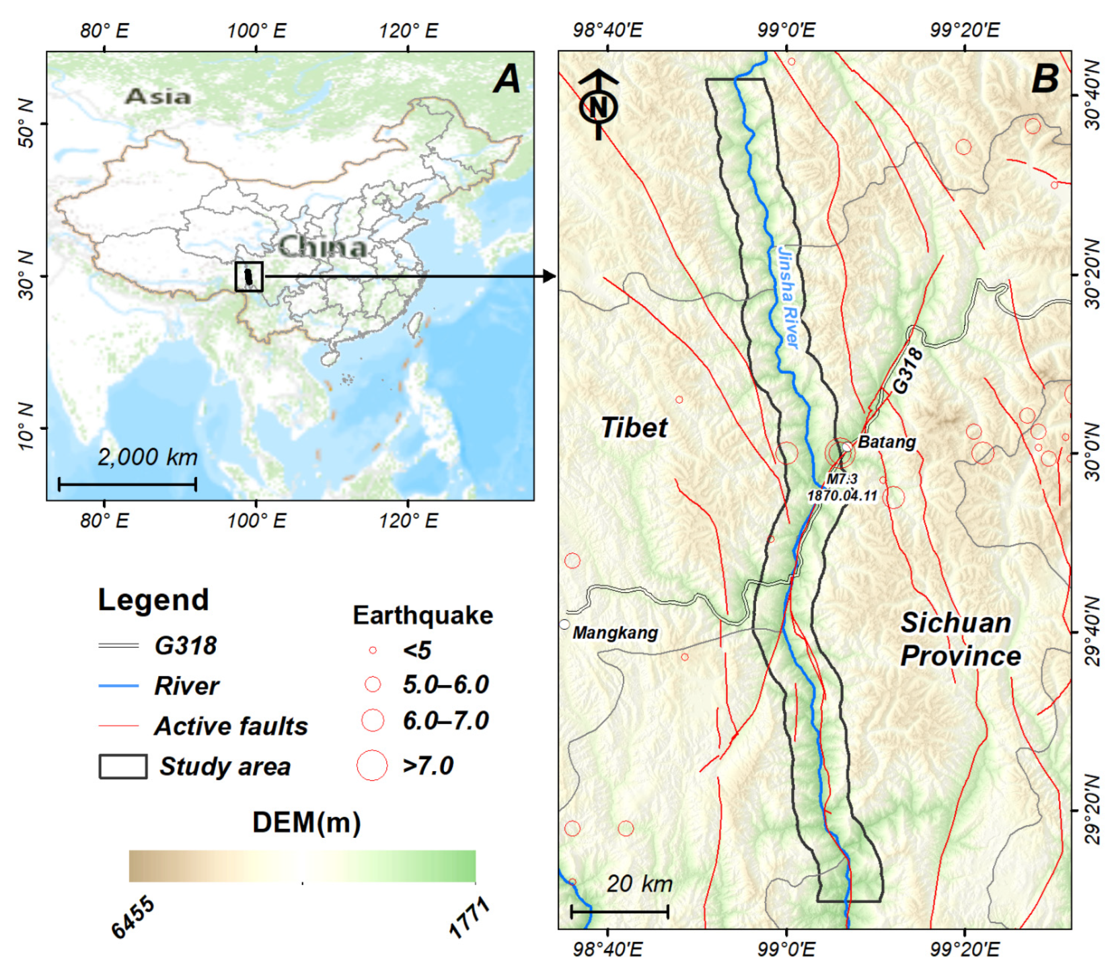
In this study, we selected the Batang section of Jinsha River (about 1832 km2) in China as the study area (as shown in Figure 2). The Jinsha River is the upper reaches of the Yangtze River, characterized by huge elevation differences and deep valleys. Due to tectonic movements, a series of north–south active faults have developed around the study area. Historically, several large earthquakes occurred here, such as the magnitude 7.3 earthquake in 1870. The combination of multiple factors makes landslide disasters in the study area very frequent. A typical case of recent disasters is that in October 2018, two collapses of the Baige landslide occurred within a month, damming the Jinsha River twice [4]. These two landslide events caused catastrophic flooding that threatened people’s lives and caused significant economic losses. Thus, there is an urgent need for the rapid mapping and updating of landslides in this area to prevent the occurrence of similar disasters.
Through the ASF data platform, we first retrieved 352 Sentinel-1 images for ascending and descending tracks from January 2018 to December 2021. To reduce the effect of temporal and spatial decoherence, the perpendicular and temporal baselines should be set relatively small. According to the options provided by HyP3 platform, the maximum temporal baseline for this study was set to 36 days, and the maximum perpendicular baseline was set to 200 m. We, therefore, created three InSAR processing flows containing a total of 923 interferometric pairs. The detailed data usage is shown in Table 1.
Subsequently, these interferometric pairs were submitted to the HyP3 online platform for InSAR data processing. The number of looks was set to 10 × 2, allowing results with a pixel spacing of 40 m. After downloading the processed products, we manually checked the interferograms one-by-one to ensure their completeness and estimated the data error of each interferometric pair to ensure their availability. The unwrapped interferograms with good coherence were, therefore, selected. Finally, we adopted the MintPy tool to perform the Stacking-InSAR processing.
In addition, Google Earth images (2 m) and DEM (12.5 m) were also collected to assist Stacking-InSAR results in identifying slow-moving landslides. The DEM data are from ALOS PALSAR DEM products and can be downloaded from the ASF website.
4. Results and Validation
4.1. Slow-Moving Landslide Mapping
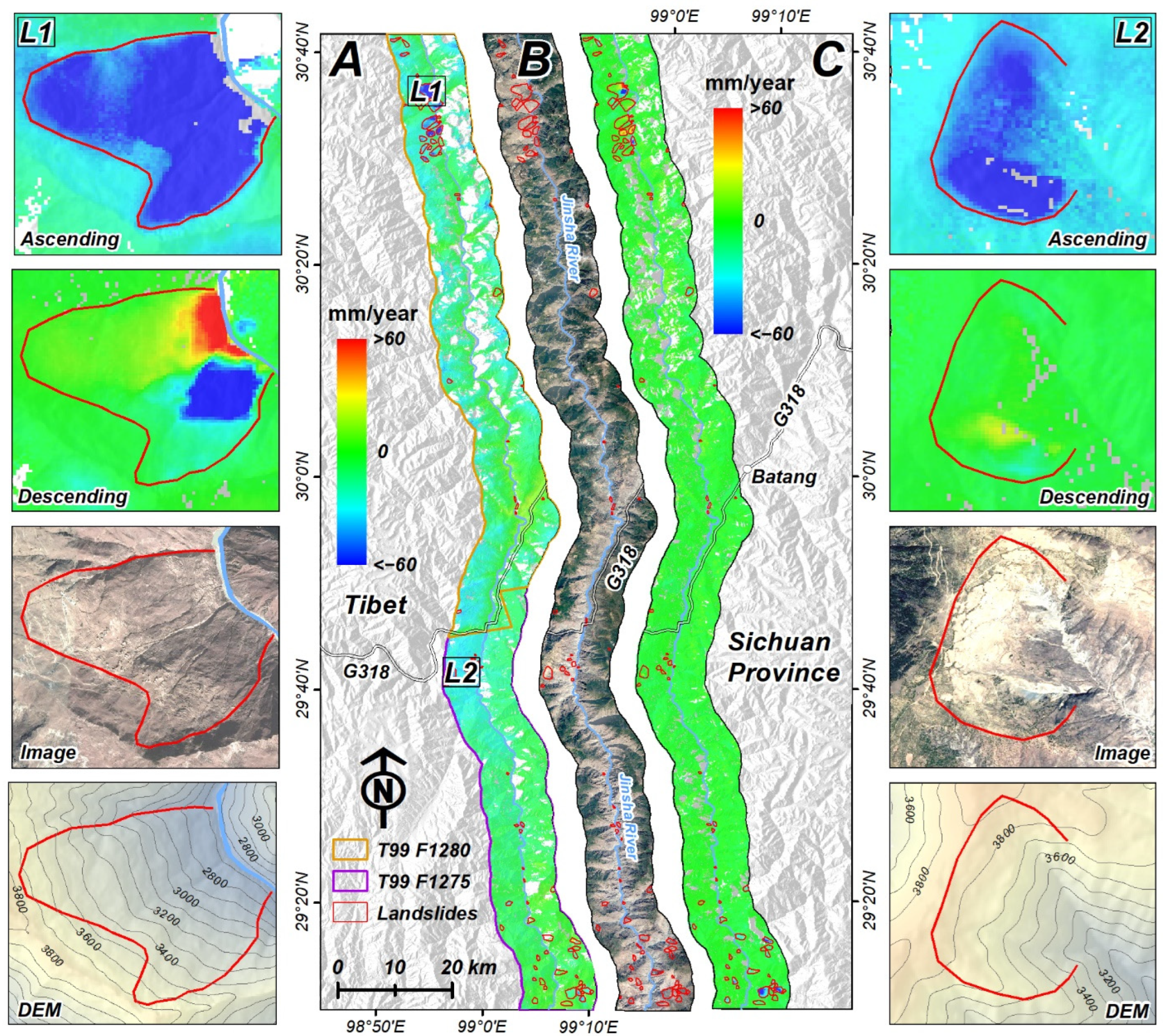
Figure 3 presents the Stacking-InSAR results for the study area. Note that the average deformation rate (mm/year) is in the line-of-sight (LOS) direction. A positive value indicates the movement close to the satellite (red color) and vice versa for negative value (blue color). According to [39], the scatterers were corrupted by the strong noise when the absolute value of the LOS velocity was below 6–7 mm/year. Thus, in this study, we mainly interpreted the scatterers with deformation rate greater than 10 mm/year.
A total of 81 slow-moving landslides were identified and mapped. The landslide areas ranged from about 0.05 km2 to more than 5 km2, with an average area of about 0.6 km2. The total area of identified slow-moving landslides was nearly 50 km2. Most of the mapped slow-moving landslides were distributed along the Jinsha River. Optically, most of them were old landslides that have historically failed.
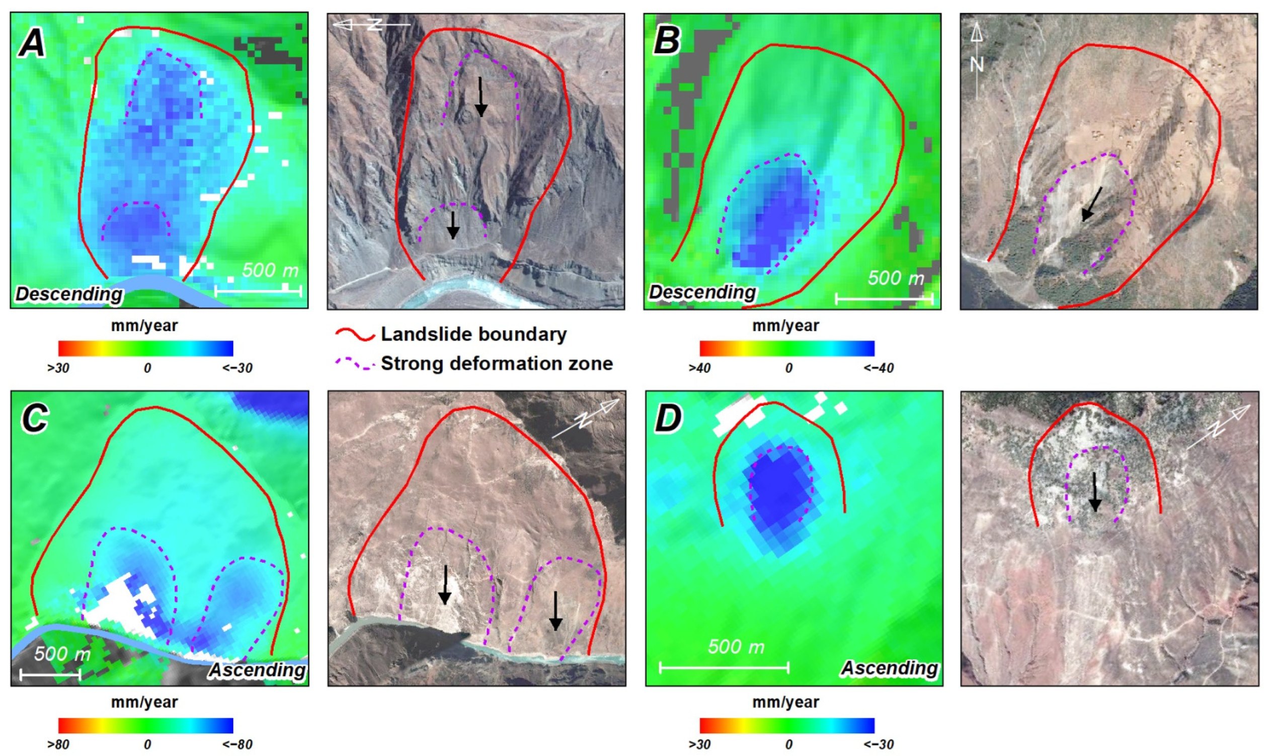
Figure 4 illustrates the annual deformation rate of four typical slow-moving landslides from 2018 to 2021. For Figure 4A, the whole landslide was in motion during the monitoring period, with a maximum LOS velocity exceeding 30 mm/year. Moreover, its characteristics can be clearly seen from the optical image, and its front edge close to the Jinsha River has begun to partially collapse, with evident cracks appearing. For Figure 4B, the significant deformation part of this landslide is located at its front edge, with a maximum LOS velocity exceeding 40 mm/year. The grayish-white slip wall and the loose accumulation on its front edge are clearly visible on the optical image. It appears to be a pull-type landslide, with the sliding rate at the rear being significantly less than that at the front. In addition, it is worth noting that the slope at the middle of the landslide body is relatively gentle, with some buildings. Once the landslide fails, these buildings will be at risk of damage. For Figure 4C, the landslide, shaped similar to a lap chair, has a large sliding rate at the front edge, with a maximum LOS velocity exceeding 80 mm/year. The damage characteristics of its front edge can also be clearly seen on the optical image. For Figure 4D, the LOS velocity at the top of the landslide exceeds 30 mm/year. The deformation area is mainly located at the top of the gully and visible signs of damage can also be seen from the optical image. Under the effect of heavy rainfall, it is likely to evolve into a source of mudslides. Overall, landslide boundaries identified based on the average velocity maps are in good agreement with corresponding geomorphological features, implying that the InSAR-driven landslide identification results are reliable.
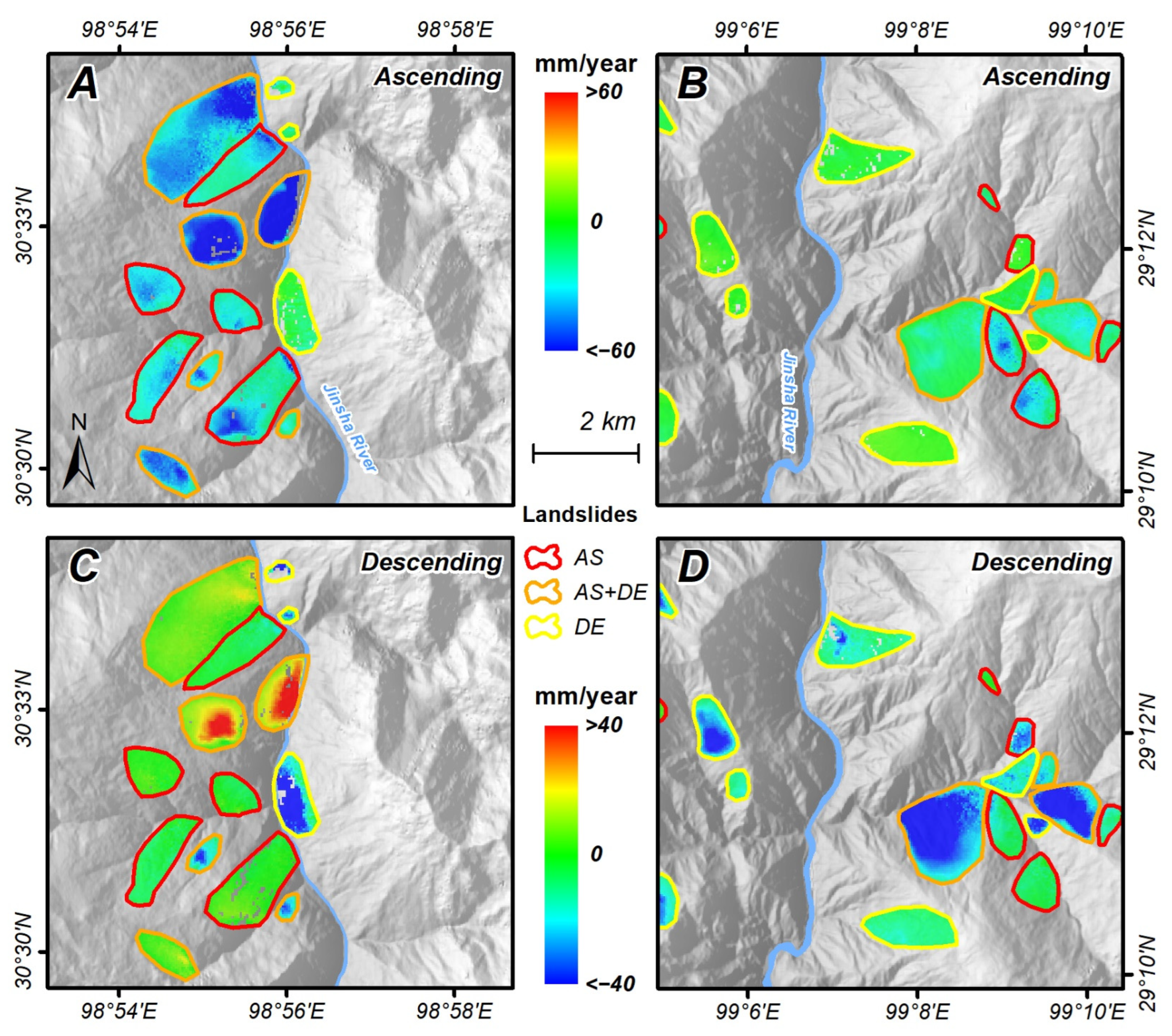
As shown in Figure 5, it can be seen that landslides with larger deformations are shown on both ascending and descending results, while landslides with smaller deformation only visible on a single track. Of these identified landslides, 51 were identified using the ascending track, and 52 were identified using the descending track. The number of landslides identified using the ascending and descending tracks is approximately equal, accounting for about 64% of the total number identified. In addition, 22 slow-moving landslides are identified from both the ascending and descending tracks, only 27% of the total. Evidently, the combination of ascending and descending data can effectively reduce landslide identification omissions, especially in mountainous areas. Moreover, the results of ascending and descending tracks can also be confirmed with each other, although the number of their overlap is small. Additionally, due to the characteristics of SAR imaging, there is a certain difference in the deformation rate of the same slope driven by ascending and descending tracks. For quantitative analysis, we can decompose the slope deformation by using the ascending and descending data to obtain the real motion of the slope. Thus, we recommend using both ascending and descending track data for mapping landslides in mountainous areas when data are available.
4.2. Comparison with Existing Landslide Inventories
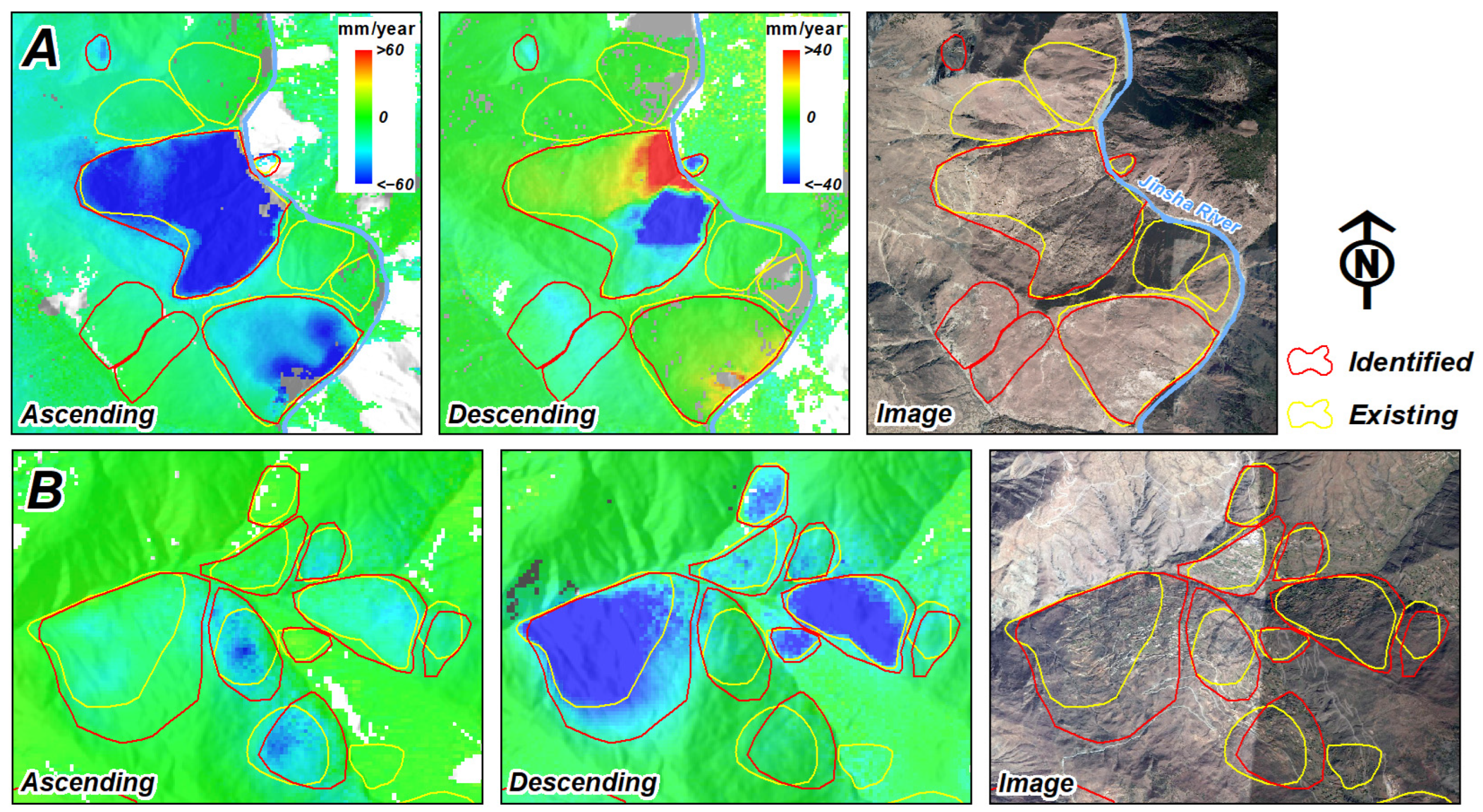
To further validate the mapped results, we compared each identified slow-moving landslide with previous identifications in the study area. In the study area, a total of 90 landslides were detected by using Sentinel-1 (ascending and descending) and ALOS PALSAR-1 (ascending) data from 2007 to 2019, and these slow-moving landslides were also confirmed by optical images [24,40]. Thus, they can be considered as relatively complete landslide inventories covering the study area. We identified 65 of these landslides, although the identified landslide boundaries did not completely overlap (as shown in Figure 6). There were 25 landslides that we did not identify. In addition, we detected 16 new landslides that were not in the previous results. There are several possible reasons for this discrepancy. For instance, we used Sentinel-1 data from 2018 to 2021 and did not use ALOS PALSAR-1 data. Moreover, the movement state of landslides may not be the same at different time periods, which is a long-term cumulative non-linear deformation. In any case, a recognition overlap rate of more than 70% is sufficient to prove that our identification results are reliable.
Overall, the new processing chain is reliable and effective for wide-area landslide mapping, which can be used as a powerful tool to quickly update the existing landslide inventories.
5. Discussion
5.1. Error Estimation of Interferograms
Estimating the quality of interferograms is a crucial step before applying them. In this study, we directly characterized the data errors by estimating the mean and standard deviation of each interferogram. To avoid estimation bias, we randomly selected several areas in the low-slope (less than 15 degrees) regions for error estimation. The main assumption of this step is that low-slope areas are less prone to landslides and, therefore, have little expected deformation.
Figure 7A shows the mean and standard deviation of each interferogram. We found that the absolute values of the means of all interferograms were within 0.5 mm and the standard deviations were within 5 mm. These residual values were acceptable considering the observation error of InSAR and the fact that we did not perform any additional error corrections (e.g., orbital errors, tropospheric errors, and topographic errors) [41]. This indicated that the interferograms derived from the HyP3 online platform were applicable and effective for landslide mapping.
Subsequently, we calculated the average value of spatial coherence of these interferograms, as shown in Figure 7B. To ensure the quality of the Stacking-InSAR results, the interferogram with average spatial coherence values below 0.5 were discarded. In total, there were 46 interferometric pairs with average spatial coherence below 0.5, i.e., 23 in T99 F1280, 12 in T99 F1275, and 11 in T33 F493. Therefore, there were actually 877 interferograms involved in the Stacking-InSAR processing.
5.2. Visibility Analysis of SAR Satellites
Based on the R-index, we analyzed the terrain visibility of the study area, as shown in Figure 8. For the ascending track, 6.25% of the study area was affected by the layover and shadow (poor visibility), 45.08% was affected by foreshortening (medium visibility), and the remaining 48.67% of the study area had good visibility. Similar to the ascending track, the percentage of areas with poor, medium, and good visibility for the descending track was 6.10%, 43.85%, and 50.05%, respectively. Apparently, the study area was less affected by the layover and shadow. In this study, to avoid misidentification, the layover and shadow areas were masked out before mapping the landslides. For the surface deformation in the foreshortening area, we combined optical images to comprehensively identify landslides. Even in this case, the number of landslides identified using a single track (ascending or descending) only accounted for about 64% of the total number of landslides. Therefore, it is strongly recommended to use the combination of ascending and descending tracks for landslide detection in mountainous areas to obtain a more complete landslide inventory.
5.3. Advantages and Limitations
In this study, we presented a case study of slow-moving landslide mapping over large areas by using a new landslide mapping chain. We summarized that the new landslide mapping chain has three main advantages.
First of all, it is very easy to use without complicated data processing skills. This is mainly due to the convenience of HyP3 and the simplicity of Stacking-InSAR method. Moreover, the whole processing chain is open source and nearly automatic, thus users do not need to install and master complex commercial processing software to receive reliable results. In addition, ref. [23] confirmed the effectiveness of the Stacking-InSAR method in low coherence areas, which can be applied to mountain areas with dense vegetation.
Second, it greatly reduces data processing time. In fact, it is one of the main advantages of the HyP3 and Stacking-InSAR method. With HyP3, it took only 4–5 h to process a total of 923 interferometric pairs. However, in a normal workstation environment (Intel Xeon Gold 6152 CPU, 32 G memory), we estimated that it would take at least 1–2 months to process these interferometric pairs. It is almost unbearable for practical applications, especially in emergency response. Moreover, the time spent by the Stacking-InSAR method is almost negligible (several minutes) because it does not require any additional processing. However, if SBAS-InSAR is adopted, it may take several hours to process.
Third, it greatly saves storage resources, although it is a significant advantage of the HyP3 online platform. For this study, a total of 923 interferometric pairs occupied less than 1 terabyte (TB) of storage space, compared to 15–20 TB that might be required for conventional processing. It is a huge advantage for large-scale data processing.
In addition, in the absence of a priori knowledge of landslide distribution, the new processing chain can rapidly identify the landslide distribution area and narrow the study area to save the time of conventional InSAR processing. Therefore, this processing chain can also be regarded as a prior experiment of conventional InSAR processing.
Undoubtedly, the new processing chain also has some limitations. An important limitation is that HyP3 does not support arbitrary adjustment of parameters during the interferometric processing (such as filtering parameters, phase unwrapping methods), meaning that we may sometimes not obtain the desired results. For instance, the HyP3 online platform only supports the output of products with a pixel spacing of 40 m or 80 m. For landslide detection, it means that some small-scale landslides may be missed. Moreover, the HyP3 platform sets a monthly processing quota, meaning that each user can only process a given number of interference pairs per month (1000 jobs/month), although, in most cases, it is sufficient for a region.
In addition, we mainly focused on the rapid identification of wide-area landslides, which means that we only performed the stacking of interferograms without any additional processing, such as atmospheric correction, topography correction, etc. A recent study reported that atmospheric correction of interferograms prior to the implementation of Stacking-InSAR processing would help to improve the deformation accuracy, especially when processing SAR images over large areas [42]. We will perform this process in the future to further improve the landslide mapping chain. Moreover, for time-series landslide analysis, the Stacking-InSAR method still has some limitations. In terms of this aspect, users can replace the Stacking-InSAR method with SBAS-InSAR or another time-series InSAR method as needed to obtain time-series landslide deformation data.
Finally, the deformation signal observed by InSAR may be caused by various earth movements [41], not just landslides. In this case, to avoid misidentification, the optical and geomorphological features of landslides need to be considered together when using InSAR-driven surface deformations to interpret landslides. Moreover, the InSAR method can only detect deformation regions, not the whole landslide boundary. Thus, the use of high-resolution optical imagery can also help to finely delineate the landslide boundary.
Overall, the new landslide mapping chain is very suitable for the rapid detection of slow-moving landslides over large areas. In the future, we expect to use this processing chain to identify and update landslide inventory maps for more areas around the world to further promote the understanding of landslide hazards.
6. Conclusions
Almost every country or region in the world is potentially threatened by landslide hazards. Identifying slow-moving landslides in advance is considered as a critical step for prevention and management of landslide hazards. However, rapid identification of slow-moving landslides over large areas is difficult and challenging. In this work, we constructed a new easy-to-use processing chain for rapidly identifying slow-moving landslides over large areas, by combining the HyP3 online platform and Stacking-InSAR method.
With this new processing chain, we obtained a total of 923 interferograms covering an area of over 1800 km2 within a few hours and identified a total of 81 slow-moving landslides. Among them, 65 were confirmed by previous studies, and 16 landslides were newly detected. The effectiveness of the new processing chain was confirmed. The results showed that the new landslide mapping chain greatly simplifies the process of wide-area landslide mapping, which can be used as an effective tool to update the existing landslide inventories and contribute to the prevention and management of geological hazards.
Author Contributions
Conceptualization, Y.Y. and X.X.; methodology, Y.Y. and G.X.; software, Y.Y. and G.X.; validation, Y.Y. and H.G.; formal analysis, Y.Y.; investigation, H.G.; resources, Y.Y.; data curation, Y.Y.; writing—original draft preparation, Y.Y.; writing—review and editing, G.X. and H.G.; visualization, Y.Y.; supervision, X.X.; project administration, Y.Y.; funding acquisition, X.X. All authors have read and agreed to the published version of the manuscript.
Funding
This research was funded by the National Natural Science Foundation of China (grant number: 41941016, U1839204, U2139201, 41572193 and 42104008) and the National Institute of Natural Hazards, Ministry of Emergency Management of China Research Fund (ZDJ2018-22).
Data Availability Statement
Not applicable.
Acknowledgments
We are very grateful for the HyP3 online platform and the open-source MintPy tool. The InSAR products were processed by the ASF DAAC HyP3 2022 using the hyp3_gamma plugin version 5.4.4 running GAMMA release 20210701. This work contains modified Copernicus Sentinel data 2019, processed by ESA. In addition, we are also very grateful to Yao Xin for providing existing landslide inventories in the study area, and Ren Junjie for providing the facility support.
Conflicts of Interest
The authors declare no conflict of interest.
References
- Haque, U.; da Silva, P.F.; Devoli, G.; Pilz, J.; Zhao, B.; Khaloua, A.; Wilopo, W.; Andersen, P.; Lu, P.; Lee, J.; et al. The human cost of global warming: Deadly landslides and their triggers (1995–2014). Sci. Total Environ. 2019, 682, 673–684. [Google Scholar] [CrossRef]
- Tsai, F.; Hwang, J.H.; Chen, L.C.; Lin, T.H. Post-disaster assessment of landslides in southern Taiwan after 2009 Typhoon Morakot using remote sensing and spatial analysis. Nat. Hazards Earth Syst. Sci. 2010, 10, 2179–2190. [Google Scholar] [CrossRef] [Green Version]
- Hu, K.; Wu, C.; Tang, J.; Pasuto, A.; Li, Y.; Yan, S. New understandings of the June 24th 2017 Xinmo Landslide, Maoxian, Sichuan, China. Landslides 2018, 15, 2465–2474. [Google Scholar] [CrossRef] [Green Version]
- Fan, X.; Xu, Q.; Alonso-Rodriguez, A.; Subramanian, S.S.; Li, W.; Zheng, G.; Dong, X.; Huang, R. Successive landsliding and damming of the Jinsha River in eastern Tibet, China: Prime investigation, early warning, and emergency response. Landslides 2019, 16, 1003–1020. [Google Scholar] [CrossRef]
- Xu, Q. Understanding and Consideration of Related Issues in Early Identification of Potential Geohazards. Geomat. Inf. Sci. Wuhan Univ. 2020, 45, 1651–1659. [Google Scholar]
- Emberson, R.; Kirschbaum, D.; Stanley, T. Global connections between El Nino and landslide impacts. Nat. Commun. 2021, 12, 2262. [Google Scholar] [CrossRef]
- Crozier, M.J. Deciphering the effect of climate change on landslide activity: A review. Geomorphology 2010, 124, 260–267. [Google Scholar] [CrossRef]
- Lacroix, P.; Handwerger, A.L.; Bièvre, G. Life and death of slow-moving landslides. Nat. Rev. Earth Environ. 2020, 1, 404–419. [Google Scholar] [CrossRef]
- Hungr, O.; Leroueil, S.; Picarelli, L. The Varnes classification of landslide types, an update. Landslides 2014, 11, 167–194. [Google Scholar] [CrossRef]
- Gabriel, A.K.; Goldstein, R.M.; Zebker, H.A. Mapping small elevation changes over large areas: Differential radar interferometry. J. Geophys. Res. 1989, 94, 9183–9191. [Google Scholar] [CrossRef]
- Ferretti, A.; Prati, C.; Rocca, F. Permanent scatterers in SAR interferometry. IEEE Trans. Geosci. Remote Sens. 2001, 39, 8–20. [Google Scholar] [CrossRef]
- Berardino, P.; Fornaro, G.; Lanari, R.; Sansosti, E. A new algorithm for surface deformation monitoring based on small baseline differential SAR interferograms. IEEE Trans. Geosci. Remote Sens. 2002, 40, 2375–2383. [Google Scholar] [CrossRef] [Green Version]
- Casu, F.; Manzo, M.; Lanari, R. A quantitative assessment of the SBAS algorithm performance for surface deformation retrieval from DInSAR data. Remote Sens. Environ. 2006, 102, 195–210. [Google Scholar] [CrossRef]
- Li, S.; Xu, W.; Li, Z. Review of the SBAS InSAR Time-series algorithms, applications, and challenges. Geod. Geodyn. 2022, 13, 114–126. [Google Scholar] [CrossRef]
- Osmanoğlu, B.; Sunar, F.; Wdowinski, S.; Cabral-Cano, E. Time series analysis of InSAR data: Methods and trends. ISPRS J. Photogramm. Remote Sens. 2016, 115, 90–102. [Google Scholar] [CrossRef]
- Qu, F.; Lu, Z.; Kim, J.; Turco, M.J. Mapping and characterizing land deformation during 2007–2011 over the Gulf Coast by L-band InSAR. Remote Sens. Environ. 2023, 284, 113342. [Google Scholar] [CrossRef]
- Pourkhosravani, M.; Mehrabi, A.; Pirasteh, S.; Derakhshani, R. Monitoring of Maskun landslide and determining its quantitative relationship to different climatic conditions using D-InSAR and PSI techniques. Geomat. Nat. Hazards Risk 2022, 13, 1134–1153. [Google Scholar] [CrossRef]
- Dai, K.; Li, Z.; Xu, Q.; Burgmann, R.; Milledge, D.G.; Tomas, R.; Fan, X.; Zhao, C.; Liu, X.; Peng, J.; et al. Entering the Era of Earth Observation-Based Landslide Warning Systems: A Novel and Exciting Framework. IEEE Geosci. Remote Sens. Mag. 2020, 8, 136–153. [Google Scholar] [CrossRef] [Green Version]
- Mondini, A.C.; Guzzetti, F.; Chang, K.-T.; Monserrat, O.; Martha, T.R.; Manconi, A. Landslide failures detection and mapping using Synthetic Aperture Radar: Past, present and future. Earth-Sci. Rev. 2021, 216, 103574. [Google Scholar] [CrossRef]
- Tsironi, V.; Ganas, A.; Karamitros, I.; Efstathiou, E.; Koukouvelas, I.; Sokos, E. Kinematics of Active Landslides in Achaia (Peloponnese, Greece) through InSAR Time Series Analysis and Relation to Rainfall Patterns. Remote Sens. 2022, 14, 844. [Google Scholar] [CrossRef]
- Kang, Y.; Lu, Z.; Zhao, C.; Xu, Y.; Kim, J.-W.; Gallegos, A.J. InSAR monitoring of creeping landslides in mountainous regions: A case study in Eldorado National Forest, California. Remote Sens. Environ. 2021, 258, 112400. [Google Scholar] [CrossRef]
- Bekaert, D.P.S.; Handwerger, A.L.; Agram, P.; Kirschbaum, D.B. InSAR-based detection method for mapping and monitoring slow-moving landslides in remote regions with steep and mountainous terrain: An application to Nepal. Remote Sens. Environ. 2020, 249, 111983. [Google Scholar] [CrossRef]
- Zhang, L.; Dai, K.; Deng, J.; Ge, D.; Liang, R.; Li, W.; Xu, Q. Identifying Potential Landslides by Stacking-InSAR in Southwestern China and Its Performance Comparison with SBAS-InSAR. Remote Sens. 2021, 13, 3662. [Google Scholar] [CrossRef]
- Xin, Y.; Jianhui, D.; Xinghong, L.; Zhenkai, Z.; Jiaming, Y.; Fuchu, D.; Kaiyu, R.; Lingjing, L. Primary Recognition of Active Landslides and Development Rule Analysis for Pan Three-river-parallel Territory of Tibet Plateau. Adv. Eng. Sci. 2020, 52, 16–37. [Google Scholar]
- Cook, M.E.; Brook, M.S.; Hamling, I.J.; Cave, M.; Tunnicliffe, J.F.; Holley, R. Investigating slow-moving shallow soil landslides using Sentinel-1 InSAR data in Gisborne, New Zealand. Landslides 2022, 20, 427–446. [Google Scholar] [CrossRef]
- Yazici, B.V.; Tunc Gormus, E. Investigating persistent scatterer InSAR (PSInSAR) technique efficiency for landslides mapping: A case study in Artvin dam area, in Turkey. Geocarto Int. 2020, 37, 2293–2311. [Google Scholar] [CrossRef]
- Festa, D.; Bonano, M.; Casagli, N.; Confuorto, P.; De Luca, C.; Del Soldato, M.; Lanari, R.; Lu, P.; Manunta, M.; Manzo, M.; et al. Nation-wide mapping and classification of ground deformation phenomena through the spatial clustering of P-SBAS InSAR measurements: Italy case study. ISPRS J. Photogramm. Remote Sens. 2022, 189, 1–22. [Google Scholar] [CrossRef]
- Li, Y.; Jiang, W.; Zhang, J. A time series processing chain for geological disasters based on a GPU-assisted sentinel-1 InSAR processor. Nat. Hazards 2021, 111, 803–815. [Google Scholar] [CrossRef]
- Morishita, Y.; Lazecky, M.; Wright, T.; Weiss, J.; Elliott, J.; Hooper, A. LiCSBAS: An Open-Source InSAR Time Series Analysis Package Integrated with the LiCSAR Automated Sentinel-1 InSAR Processor. Remote Sens. 2020, 12, 424. [Google Scholar] [CrossRef] [Green Version]
- Hogenson, K.; Kristenson, H.; Kennedy, J.; Johnston, A.; Rine, J.; Logan, T.A.; Zhu, J.; Williams, F.; Herrmann, J.; Smale, J.; et al. Hybrid Pluggable Processing Pipeline (HyP3): A Cloud-Native Infrastructure for Generic Processing of SAR Data. In Proceedings of the 2016 AGU Fall Meeting, San Francisco, CA, USA, 12–16 December 2016. [Google Scholar]
- Weiss, J.R.; Walters, R.J.; Morishita, Y.; Wright, T.J.; Lazecky, M.; Wang, H.; Hussain, E.; Hooper, A.J.; Elliott, J.R.; Rollins, C.; et al. High-Resolution Surface Velocities and Strain for Anatolia From Sentinel-1 InSAR and GNSS Data. Geophys. Res. Lett. 2020, 47, e2020GL087376. [Google Scholar] [CrossRef]
- Agapiou, A.; Lysandrou, V. Detecting Displacements Within Archaeological Sites in Cyprus After a 5.6 Magnitude Scale Earthquake Event Through the Hybrid Pluggable Processing Pipeline (HyP3) Cloud-Based System and Sentinel-1 Interferometric Synthetic Aperture Radar (InSAR) Analysis. IEEE J. Sel. Top. Appl. Earth Obs. Remote Sens. 2020, 13, 6115–6123. [Google Scholar] [CrossRef]
- Nicolau, A.P.; Flores-Anderson, A.; Griffin, R.; Herndon, K.; Meyer, F.J. Assessing SAR C-band data to effectively distinguish modified land uses in a heavily disturbed Amazon forest. Int. J. Appl. Earth Obs. Geoinf. 2021, 94, 102214. [Google Scholar] [CrossRef]
- Yunjun, Z.; Fattahi, H.; Amelung, F. Small baseline InSAR time series analysis: Unwrapping error correction and noise reduction. Comput. Geosci. 2019, 133, 104331. [Google Scholar] [CrossRef] [Green Version]
- Sandwell, D.T.; Price, E.J. Phase gradient approach to stacking interferograms. J. Geophys. Res. Solid Earth 1998, 103, 30183–30204. [Google Scholar] [CrossRef] [Green Version]
- Kang, Y.; Zhao, C.; Zhang, Q.; Lu, Z.; Li, B. Application of InSAR Techniques to an Analysis of the Guanling Landslide. Remote Sens. 2017, 9, 1046. [Google Scholar] [CrossRef] [Green Version]
- Ren, T.; Gong, W.; Bowa, V.M.; Tang, H.; Chen, J.; Zhao, F. An Improved R-Index Model for Terrain Visibility Analysis for Landslide Monitoring with InSAR. Remote Sens. 2021, 13, 1938. [Google Scholar] [CrossRef]
- Notti, D.; Herrera, G.; Bianchini, S.; Meisina, C.; García-Davalillo, J.C.; Zucca, F. A methodology for improving landslide PSI data analysis. Int. J. Remote Sens. 2014, 35, 2186–2214. [Google Scholar] [CrossRef]
- Kovács, I.P.; Bugya, T.; Czigány, S.; Defilippi, M.; Lóczy, D.; Riccardi, P.; Ronczyk, L.; Pasquali, P. How to avoid false interpretations of Sentinel-1A TOPSAR interferometric data in landslide mapping? A case study: Recent landslides in Transdanubia, Hungary. Nat. Hazards 2018, 96, 693–712. [Google Scholar] [CrossRef] [Green Version]
- Xin, Y. Active Landslides by InSAR Recognition in Three-River-Parallel Territory of Qinghai-Tibet Plateau (2007–2019). 2022. Available online: https://poles.tpdc.ac.cn/en/data/a0c9b7cb-3184-4214-990d-76dc27aa2722/?q= (accessed on 10 June 2022).
- Stephenson, O.L.; Liu, Y.K.; Yunjun, Z.; Simons, M.; Rosen, P.; Xu, X. The Impact of Plate Motions on Long-Wavelength InSAR-Derived Velocity Fields. Geophys. Res. Lett. 2022, 49, e2022GL099835. [Google Scholar] [CrossRef]
- Xiao, R.; Yu, C.; Li, Z.; Jiang, M.; He, X. InSAR stacking with atmospheric correction for rapid geohazard detection: Applications to ground subsidence and landslides in China. Int. J. Appl. Earth Obs. Geoinf. 2022, 115, 103082. [Google Scholar] [CrossRef]
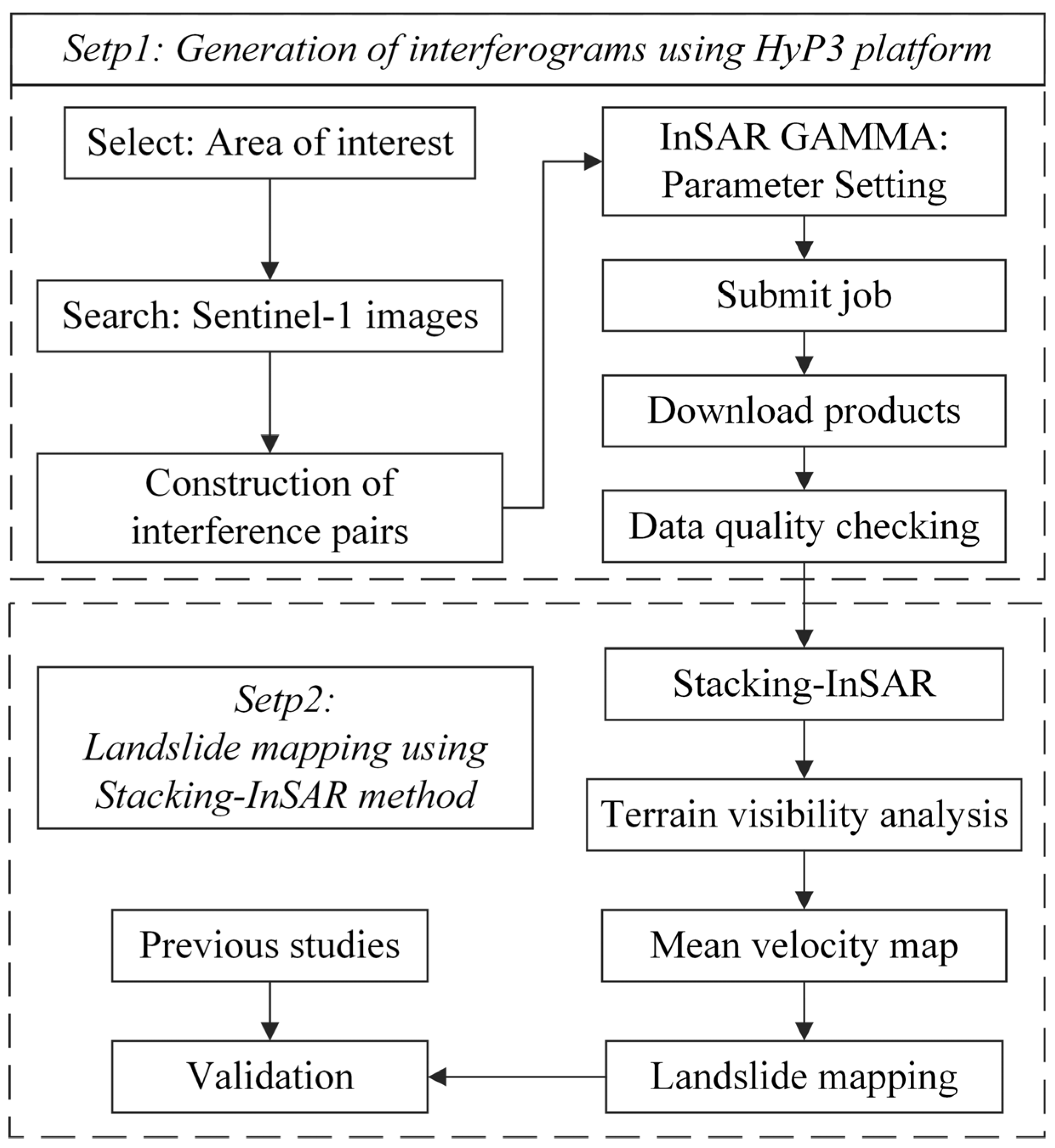
Figure 1.
The new rapid landslide mapping chain used in this study.

Figure 2.
Map of the study area. (A) The geographical location of the study area, (B) Tectonic and topographic map of the study area. Red lines show major active faults, and red circles show major earthquakes.
Figure 2.
Map of the study area. (A) The geographical location of the study area, (B) Tectonic and topographic map of the study area. Red lines show major active faults, and red circles show major earthquakes.

Figure 3.
The LOS velocity of the study area and optical images. (A) LOS velocity of ascending track, (B) Optical images obtained from Google Earth, (C) LOS velocity of ascending track. The four black rectangles on the left and right show the LOS velocity maps, optical features, and topography of two typical landslides (L1 and L2 in (A)), respectively. The hill shade data calculated from DEM is used as the base map.

Figure 4.
The LOS velocity and optical features of four typical slow-moving landslides. (A,B) LOS velocity of descending track, (C,D) LOS velocity of ascending track. The red lines show the landslide boundary, the purple lines show the strong deformation zone of the landslide determined by the LOS velocity, and the black arrows indicate the sliding direction of the landslide.

Figure 5.
Comparison of LOS velocity maps for ascending (A,B) and descending (C,D) tracks of typical landslides. For clarity, the hill shade data calculated from DEM is used as the base map.
Figure 5.
Comparison of LOS velocity maps for ascending (A,B) and descending (C,D) tracks of typical landslides. For clarity, the hill shade data calculated from DEM is used as the base map.

Figure 6.
Comparison of landslide identification results for two typical areas with the existing landslide inventories. (A,B) are two sub-regions of the study area. The base map of ascending and descending is the hill shade data. Optical images are from Google Earth.
Figure 6.
Comparison of landslide identification results for two typical areas with the existing landslide inventories. (A,B) are two sub-regions of the study area. The base map of ascending and descending is the hill shade data. Optical images are from Google Earth.

Figure 7.
Error estimation of all interferograms generated by the HyP3 online platform: (A) the mean and standard deviation of each interferogram, (B) average spatial coherence of each interferogram. Note that the horizontal axis only shows partial interferometric pairs.
Figure 7.
Error estimation of all interferograms generated by the HyP3 online platform: (A) the mean and standard deviation of each interferogram, (B) average spatial coherence of each interferogram. Note that the horizontal axis only shows partial interferometric pairs.

Figure 8.
R-index maps of the ascending (A) and descending (B) tracks over the study area. The black rectangles on the left and right are a zoomed-in view of the R-index maps. The visibility statistics for the ascending and descending tracks are shown in the lower left and upper right corners, respectively.


Table 1.
The Sentinel-1 images and interferograms used in this study.
| Track | Time | Number of Images | Number of Interferograms |
|---|---|---|---|
| Ascending (T99 F1280) | January 2018–December 2021 | 117 | 304 |
| Ascending (T99 F1275) | January 2018–December 2021 | 117 | 281 |
| Descending (T33 F493) | January 2018–December 2021 | 118 | 338 |
| Total | -- | 352 | 923 |
Disclaimer/Publisher’s Note: The statements, opinions and data contained in all publications are solely those of the individual author(s) and contributor(s) and not of MDPI and/or the editor(s). MDPI and/or the editor(s) disclaim responsibility for any injury to people or property resulting from any ideas, methods, instructions or products referred to in the content. |
© 2023 by the authors. Licensee MDPI, Basel, Switzerland. This article is an open access article distributed under the terms and conditions of the Creative Commons Attribution (CC BY) license (https://creativecommons.org/licenses/by/4.0/).
Share and Cite
MDPI and ACS Style
Yi, Y.; Xu, X.; Xu, G.; Gao, H. Rapid Mapping of Slow-Moving Landslides Using an Automated SAR Processing Platform (HyP3) and Stacking-InSAR Method. Remote Sens. 2023, 15, 1611. https://doi.org/10.3390/rs15061611
AMA Style
Yi Y, Xu X, Xu G, Gao H. Rapid Mapping of Slow-Moving Landslides Using an Automated SAR Processing Platform (HyP3) and Stacking-InSAR Method. Remote Sensing. 2023; 15(6):1611. https://doi.org/10.3390/rs15061611
Chicago/Turabian StyleYi, Yaning, Xiwei Xu, Guangyu Xu, and Huiran Gao. 2023. "Rapid Mapping of Slow-Moving Landslides Using an Automated SAR Processing Platform (HyP3) and Stacking-InSAR Method" Remote Sensing 15, no. 6: 1611. https://doi.org/10.3390/rs15061611
Note that from the first issue of 2016, this journal uses article numbers instead of page numbers. See further details here.