
Cloud Mesoscale Cellular Classification and Diurnal Cycle Using a Convolutional Neural Network (CNN)


1
Bay Area Environmental Research Institute, NASA Ames Research Center, Mountain View, CA 94035, USA
2
Department of Geophysics, Porter School of Environmental and Earth Sciences, Tel-Aviv University, Tel-Aviv 6997801, Israel
3
Department of Computer Sciences, Tel-Aviv University, Tel-Aviv 6997801, Israel
4
Department of Geosciences, University of Oslo, 0371 Oslo, Norway
5
Department of Atmospheric Sciences, University of Washington, Seattle, WA 98195, USA
6
Department of Physics, University of Maryland, UMBC, Baltimore, MD 21250, USA
*
Author to whom correspondence should be addressed.
Remote Sens. 2023, 15(6), 1607; https://doi.org/10.3390/rs15061607
Submission received: 26 January 2023
/
Revised: 13 March 2023
/
Accepted: 13 March 2023
/
Published: 15 March 2023
(This article belongs to the Section AI Remote Sensing)
Abstract
:Marine stratocumulus (MSC) clouds are important to the climate as they cover vast areas of the ocean’s surface, greatly affecting radiation balance of the Earth. Satellite imagery shows that MSC clouds exhibit different morphologies of closed or open mesoscale cellular convection (MCC) but many limitations still exist in studying MCC dynamics. Here, we present a convolutional neural network algorithm to classify pixel-level closed and open MCC cloud types, trained by either visible or infrared channels from a geostationary SEVIRI satellite to allow, for the first time, their diurnal detection, with a 30 min. temporal resolution. Our probability of detection was 91% and 92% for closed and open MCC, respectively, which is in line with day-only detection schemes. We focused on the South-East Atlantic Ocean during months of biomass burning season, between 2016 and 2018. Our resulting MCC type area coverage, cloud effective radii, and cloud optical depth probability distributions over the research domain compare well with monthly and daily averages from MODIS. We further applied our algorithm on GOES-16 imagery over the South-East Pacific (SEP), another semi-permanent MCC domain, and were able to show good prediction skills, thereby representing the SEP diurnal cycle and the feasibility of our method to be applied globally on different satellite platforms.
1. Introduction
Marine stratocumulus (MSC) clouds are an important component of the climate system, as they cover vast areas of the Earth’s ocean surface, they affect the radiation balance of the Earth [1], and are major contributors to the uncertainty in the changing energy budgets in climate models [2]. MSC clouds are low-level clouds that strongly reflect incoming solar radiation back to space, thereby exerting a net-negative shortwave cloud radiative effect that is primarily controlled by factors such as the cloud albedo and cloud coverage, which are properties of the open and closed mesoscale cellular convection (MCC) structure, comprising MSC clouds [3]. These two dynamic states of open and closed MCC cells are clearly observed in satellite imagery, as seen in the research domain area investigated herein (Figure 1). The cell type morphology and properties (e.g., cloud droplet number concentrations, effective radius, and precipitation rate) modulate the overall cloud coverage and albedo of the MSC cloud fields [4,5], sometimes on very short time scales. Hence, the ability to track cloud type coverage changes from space will enable us to better discern how different environmental conditions (such as different meteorological features or pollution levels, e.g., from fires) interact and affect these clouds, and how this in turn affects the Earth’s radiative budget and climate. From the remote sensing perspective, among these unique regions of open and closed MCC clouds are the semi-permanent stratocumulus cloud decks over the South-East Atlantic (SEA) Ocean, which are often overlaid by absorbing aerosols (e.g., [6]), and so adequate retrieval of aerosol properties from such regions relies on the correct assumption on the underlying cloud albedo, which is a function of the MCC cloud type [7].
To-date, several machine learning-based algorithms to detect MCC cloud types have been developed. Among the most established is the Wood and Hartmann [4] algorithm, which is based on training a MLP (Multi-Layer Perceptron) model with MODIS (Moderate Resolution Imaging Spectrometer) and the LWP (liquid water path) amount and distribution to categorize the MCC cell type on imagery patches of 256 × 256 km2. This method produces results for patches with relatively large spatial resolutions, and was shown to be useful in determining global and seasonal trends [1,2]. However, due to the algorithm utilization of cloud products derived from visible imagery and its coarse spatial resolution, its applicability for studying the dynamics and diurnal cycle of such systems is limited. Recently, a modification to this method was published [8], wherein a deep CNN (convolutional neural network) was trained on cloud-masked scene patches of 128 × 128 pixels (128 × 128 km2 close to nadir) of visible reflectance (0.55 mm) images from MODIS as their input, while producing six MCC cloud types, expanding on the Wood and Hartmann [4]’s four cloud types. Although Ref. [8] used CNN in their cloud classification, they used it as a multi-label classification (i.e., producing one class per patch), where the patch class pertains to the area surrounding the center of the patch (e.g., [9]). This method produces one cloud type class for relatively a large spatial patch (128 × 128 km2), restricts retrievals to within 45 degrees from nadir, and is limited to once-daily temporal coverage. A much finer spatial-scale segmentation approach for MCC cell type investigations was demonstrated in [3], where a watershed segmentation method was used to delineate open and closed cellular structures (order of 7 km) from GOES geostationary imagery. Their method proved to be useful for tracking open and closed cell dynamics; however, the scenes had to be classified manually a priori as closed/open cells before their utilization as inputs to the segmentation algorithm used to track cloud movement. Recently, Ref. [10] used CNN to detect pockets of open cells (POC) from MODIS imagery to come up with a long-term estimation of their occurrence over the SEA and other semi-permanent MSC locations. However, their classification was focused on larger-scale seasonal variations of only POC within an entire domain using the once-daily MODIS dataset. Our goal here was to develop a simple-to-use algorithm that can generate a MCC cloud typing with fine spatial and temporal resolutions from geostationary satellite imagery.
To achieve the goal set in this work, we utilized a fully convolutional CNN architecture (following [11,12]) to generate a semantically segmented (i.e., pixel-by-pixel) classification maps of open and closed MCC cloud types. Our algorithm was constructed to utilize single-channel (visible or infrared) high-temporal-resolution imagery (30 min) from geostationary satellites. Specifically, our algorithm was trained and used to predict 3 × 3 km2 pixel resolution images from the SEVIRI instrument onboard the MeteoSat satellite, but was also applied on the Advanced Baseline Imager (ABI) on GOES. The main contributions from this work include the following:
- Generating MSC cloud type classification on a fine temporal and spatial resolution compared with currently available products;
- The ability to generate high-temporal-resolution diurnal variability (including during the nighttime) for MCC cloud types from satellite observations;
- The algorithm was shown to be easily transformable to different satellite platforms.
This manuscript is organized in the following manner: Section 2 describes the research domain and the SEVIRI dataset used for this investigation, Section 3 describes the training and test data used in the algorithm development for both the VIS (visible) and IR (infrared) imagery, algorithm configurations, and hyperparameter tests, as well as its final configuration. Section 4 provides results from both VIS-only and IR-only trained models and discusses their comparison and validation with test data and other datasets, as well as examines MCC cloud type diurnal and seasonal variability for the research domain. In addition, it presents the applicability of the method on the GOES-ABI imagery and discusses the strengths and weaknesses of the new method, and how it may be improved for global operational applications. Section 5 discusses our work in the context of other works and steps forward.
2. Data
2.1. The Research Domain
Herein, we focused on the South-East Atlantic (SEA) Ocean domain (Figure 1), off the coast of southern West Africa (0–30°S, 20°W–10°E). This region is of special interest to the radiative and climate community because of its semi-permanent stratocumulus cloud deck, which exerts a substantial influence on regional and global radiative budget estimations and their uncertainty in climate models (e.g., [13,14]). This is especially true during the biomass burning (BB) season (Aug–Oct.), where the prevailing easterly wind transports BB aerosols from sub-Saharan Africa fire events to the SEA where the MSC cloud deck is located. This leads to a persistent above-cloud aerosol phenomenon during the BB season that is highly unique to the SEA region ([14,15,16,17]), which was specifically targeted by several international campaign efforts between 2016 and 2018, including the ORACLES (ObseRvations of Aerosols above CLouds and their intEractionS) campaign [6], CLoud–Aerosol–Radiation Interaction and Forcing: Year 2017 (CLARIFY-2017, [18]), and LASIC—Layered Atlantic Smoke Interactions with Clouds [19]. Previous studies have shown that above-cloud BB aerosols can influence the cloud water path and cloud microphysics through semi-direct and indirect effects [20,21,22,23,24]. However, this is still a topic of active research. Hence, in this work we focused on satellite measurements that corresponded to the BB season sampled during ORACLES.
2.2. SEVIRI
SEVIRI (Spinning Enhanced Visible and Infrared Imager) is the main payload of the current European Meteosat Second Generation (MSG) satellite, having 12 spectral channels, of which 8 are in the infrared with a surface resolution of 3 km at the subsatellite point. The primary location of Meteosat is at 0°E, which provides full disk images about every 12 min. In this work, we used multi-channel-calibrated and geo-rectified Level 1B products with 4 files per hour (at 15 min. intervals) downloaded from the Lille University ICARE ftp website: icare.univ-lille1.fr/SPACEBORNE/GEO/MSG+0000/L1_B (accessed on 1 November 2021). From the multi-channel NetCDF file we extracted the visible (VIS) top-of-atmosphere reflectance channels at 0.6, 0.8, and 1.6 mm (value range 0–1), and the infrared (IR) brightness temperature (BT, in Kelvin) channels of 3.9, 10.8, and 12.0 mm. To convert channel data into grayscale images, visible channels were multiplied by 255. IR images (IRscaled) were normalized according to the following equation and converted to unsigned 8-bit integers:
where BTmin and BTmax were chosen to be 270 and 295 K, respectively. These values were selected from the image histograms to represent the majority of the pixels’ ranges in the investigated domain, where most of the clouds are low level and have relatively high BT temperatures. While we used the 0.6 channel for labeling purposes, and either 0.6 (VIS) or 10.8 (clear IR) as inputs to our models, the additional channels were used as visual auxiliaries in the labeling process.
2.3. GOES-ABI
The Advanced Baseline Imager (ABI) is the primary instrument on the GOES-R Series for imaging Earth’s weather, oceans, and environment. ABI views the Earth with 16 different spectral bands, including two visible channels, four near-infrared channels, and ten infrared channels. The GOES data (GOES-16, centered on 75°W) used herein for predictions of MCC over the South-East Pacific (SEP) were taken from the ICARE ftp website under /SPACEBORNE/GEO/GOESNG-0750/L1_B/. When generating predictions with GOES, we used the IR channel (10.3 mm) as an input, scaled similarly to SEVIRI using Equation (1).
3. Methodology
3.1. Convolutional Neural Network (CNN) Models
CNN (convolutional neural network) architectures (e.g., [25]), which comprise a type of deep neural network (NN), containing multiple layers, are suited to ingest and process images, as they can perform 3D convolution operations over their n-dimensional input array (width × height × depth). Through their multiple convolutional filters, they perform feature extraction through the training process, which also preserves the spatial relationship between the pixels, thus learning image features in addition to other features including spectral ones and local ones (e.g., intensity).
CNNs have been implemented in a wealth of applications, especially in the AI (Artificial Intelligence) community (face recognition, self-driving cars), as well as with the remote sensing community, for performing image classification (e.g., [8,26,27]) or semantic segmentation (e.g., [11,12,28]). Specifically, in Ref. [8] MCC cloud prediction was based on a single class selection for a given patch (128 × 128 pixels/km2), utilizing only the encoder (i.e., feature extractor) part of a CNN architecture, as illustrated in Figure 2. However, this type of classification often does not take into account the entire surrounding spatial context. Furthermore, their prediction over an entire region (thousands of kilometers) was performed via predicting adjacent patches rather than patches with overlap, eventually resulting in a relatively sparsely classified image (as seen in their Figure 7). Here, as our goal was to classify each pixel in a given image, we utilized a fully convolutional network (FCN, [29]) in an encoder–decoder structure (Figure 2). The encoder functions as a feature extractor, while the decoder attempts to reconstruct the image labels at a scale similar to the original image by upsampling the high-level but spatially compact features, usually through 2-D transpose convolutions (also known as deconvolutional filters). As depicted in the figure, the encoder part contains multiple blocks with varying sizes and numbers of convolutional layer units and batch normalization and ReLU (rectified Linear Unit) activation function units, resulting in the contraction of the original image size. This approach is commonly used in architectures such as VGG-16 [30], ResNet [31], DeepLab [32], and FCN [29]. To obtain the semantically segmented output image, a decoder part (Figure 2) needs to be added to upsample and “de-convolve” the contracted image back to the original size. Skipping connections or “pool indices” are added between the encoder and decoder parts to allow for different-level features to be upsampled and concatenated before the final classification layer (e.g., softmax multi-class). This entire architecture structure is commonly applied in some of the most popular architectures, such as DeepLab [32] and U-Net (e.g., [33]).
3.2. Training and Test Sets
The first step in creating a CNN network is to establish a training set for the network to learn from. As this is a supervised network (i.e., learns from examples), cloud type labels need to be generated manually from the input imagery files. Figure 3 shows an example of the labeling procedure, where VIS imagery (a) was used as a reference to define cloud MCC type polygons (b) that were then converted to a discrete color class map (c). The labeling was carried out using the open-source Python labeling tool labelme [35], which allows the creation of multi-faceted polygons representing regions of mutual labels. The ground-truth maps (Figure 3c) were decoded into a PNG (portable network graphic) image file format, with discrete color numbers for each of the class types. Before carrying out the training process of the network, these numbers were converted to integer values between 0 and 3 to represent the four class types as follows: 0—other (black in the color legend), which includes ocean/background and cloud types other than MCC, 1—closed MCC (red), 2—Disorganized (disorg.) MCC (green), and 3—open MCC (yellow). For training the IR network (which uses the 10.8 mm IR imagery as input, see Figure 3d), VIS-based label maps (e.g., Figure 3c) were used as ground-truth maps.
To construct our training set, we selected 50 independent scenes (each covering a domain of 3639 × 3795 km2), sampled randomly between the months of August through October in 2016–2018 over various hours of the day (09:00–15:00 UTC), with an emphasis on allowing each year, month, and time of day to be represented. Identification of MCC cloud types was conducted manually by the authors, who are experts on the subject matter in this field. Specifically, closed MCC is characterized by close-knit cell structures, which feature high reflectivity (bright pixels), while open MCC is characterized by a honey-comb structure, with bright edges and dark inner pixels. We trained our network using 10,000 128 × 128-pixel patches selected randomly from the training dataset (42 scenes), without overlap, with 85% of the patches used for the training and 15% for validation. The remaining 8 labeled scenes were used for the final model testing. Patch sizes of 64 × 64, 128 × 128, and 256 × 256 pixels were all tested in the training process. As the patch size of 128 × 128 pixels provided the best validation accuracy, we used this as our input patch size. Note that although our input patch size was selected to be 128 × 128 pixels, the classifications were generated per pixel (i.e., 3 × 3 km2 for SEVIRI and 2 × 2 km2 for GOES-ABI).
To augment our labeled dataset used for training, we applied image augmentation routines, which include patch rotation (vertical and horizontal) variations. Brightness and contrast augmentations were tested as well, but did not yield much difference, plausibly because of the utilization of batch normalization during training.
3.3. CNN Model Setup, Architecture, and Hyperparameter Selection
Following our labeling procedure, we tested three encoder–decoder-based CNN architectures: (1) a simple (three-block) Unet, (2) a full Unet (nine blocks), and (3) a Resnet101 (encoder)–DeepLabV3 (decoder). All three were implemented through the open-source Pytorch module in Python, with the first network manually coded, and the last two using the pre-coded models in the Pytorch package, modified to fit our data input and output dimensions, without using the pre-trained weights. As the second model (a full Unet architecture) based on that of Ref. [36] provided the best results, it was used for the ensuing analysis. The uniqueness of a Unet architecture is that it has a similar number of downsample (encoder) and upsample (decoder) blocks, whereas in our simple architecture we used the total of three blocks (each with two convolution layers), and in the full Unet we had nine blocks with twenty-three overall convolutional layers [36], improving the segmentation results.
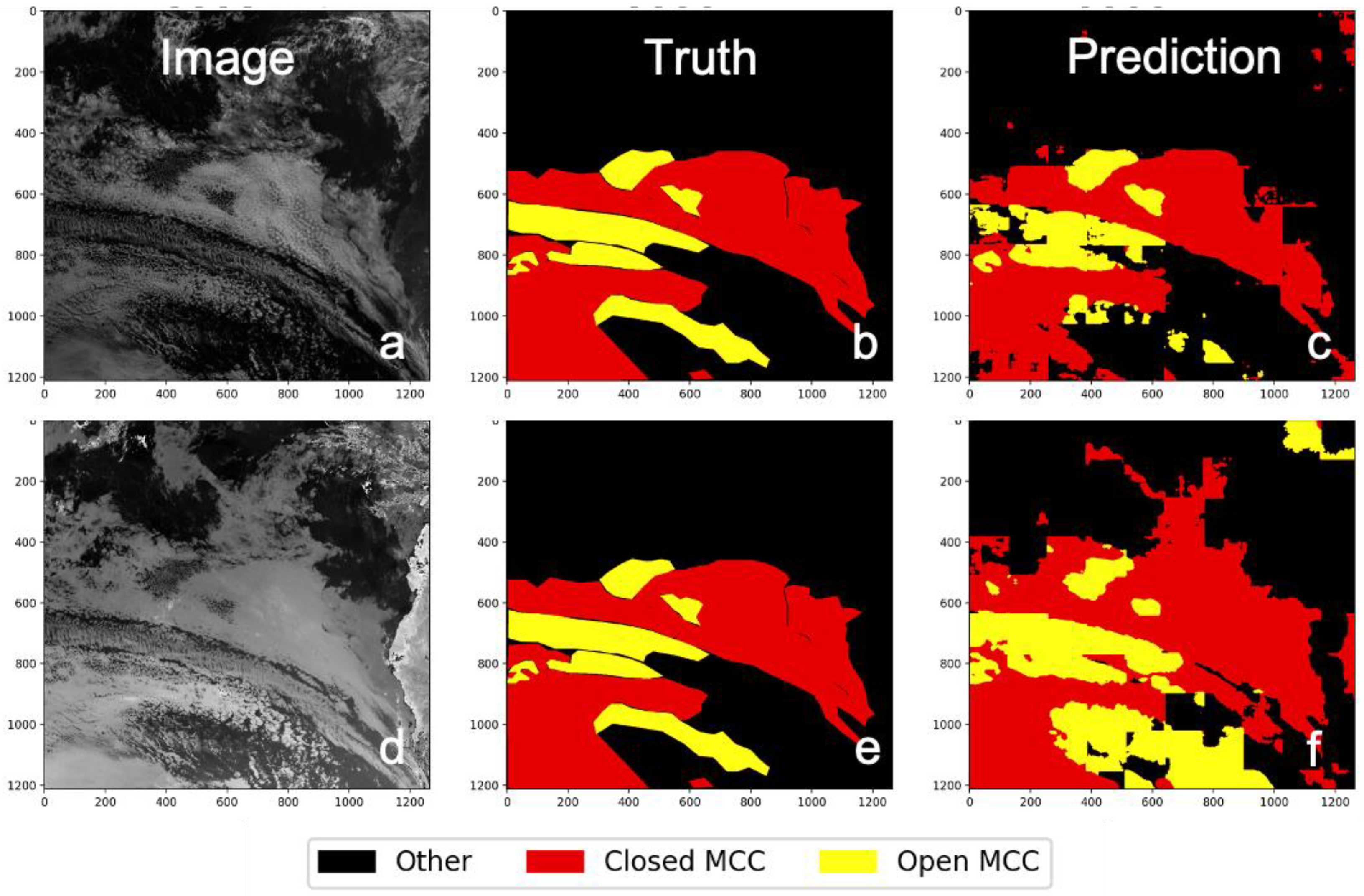
As detailed in our training procedure, we defined four classes (background/other, closed MCC, disorg. MCC, and open MCC), where the background/other class contains both the ocean background scenes and other cloud types (mid- and high-level clouds as well as other low-level clouds without a distinct organized cellular structure). As mentioned above, the closed and open MCC classes have distinct differences, with closed having a more close-knit honeycomb structure and being characterized by small cloud droplets, and open MCC has a honey-comb-like structure with a clear area in the middle, with larger effective cloud radii and smaller cloud optical thickness (COT) than the closed MCC. The disorg. MCC type is almost a hybrid version of these two types, featuring larger cells but without a distinct honey-comb structure. Moreover, it consists of small COT (like the open MCC) and small effective radii (like closed MCC). Since its structure is not well defined, its labeling can be subjective at times, which can eventually affect its prediction accuracy. Some examples of inconsistent “ground-truth” disorg. MCC labels compared with model predictions are shown in Figure 4. This model used one visible channel (0.6 mm) as an input for the four-class classification task. For this, we received an overall test set accuracy of 75%, which was driven down by the low (37%) accuracy for the disorg. MCC class type, mostly being confused with the other cloud types as shown in the figure. As the ‘other’ class type might include mid- or high-level clouds (identified from the IR channels), this might be one of the causes of mis-classification. In addition, and as seen from rows a–c in Figure 4, ground-truth disorg. MCC can feature slightly different structures (with varying sizes of “blob”-type scales), which makes their objective labeling and prediction difficult. For example, in Figure 4a–c predictions are shown on the right column, with Disorg. MCC predicted as disorg., open, and closed for panels a, b, and c, respectively. However, although the original label (generated over an entire domain scene) defined these patches as disorg., the prediction either as open or closed in panels b and c does seem correct based on the small-scale view of the selected patch. In contrast, panels d–f show ground truth as either closed or open MCC, which were partially predicted as disorg. MCC. Here, the model seemed to be predicting well based on the smaller-scale patch size (128 × 128). We also note (Figure 4f) that the predicted map was smoother than the truth map, which could also negatively bias the model prediction accuracy. Another reason for the low prediction accuracy of the disorg. MCC class is the small amount of training samples (15%), as this type represents a transition between a closed MCC structure and a less structured one.
Hence, in an attempt to improve the classes’ statistic imbalance, we used a weighted cross-entropy (CE) loss function in our next model iteration, with w = 1/S, where S is the relative proportion of each class in the training set as follows: S = [0.43 0.25 0.15 0.17]:
where x is the input, y is the target, w is the weight, C is the number of classes, and N spans a batch-size (number of samples used for training in each step of the epoch) dimension. This resulted in disorg. MCC’s accuracy improving to 47% and the open MCC-type’s test accuracy improving from 76% to 80%. Following this, we decided to combine the disorg. MCC class type with the “other/bkg” class type and concentrate our efforts on analyzing the closed MCC versus open MCC cloud type over the investigated domain, as these two MCC types are most distinct in terms of their frequency and radiative effects in the research domain.
To decide on the best network architecture and hyperparameter setup for the three-class case (after class 0 and 2 were unified), we tested several loss functions, including un-weighted CE, weighted CE, Focal Loss [37], and L2 norm, where the weighted loss CE was the only one that solved the class imbalance issue for the open MCC type. We selected the best batch-size and learning rate (LR) using a grid search over the following parameters: batch size {8,16,32,64,128,256} and LR {1 × 10⁻³, 1 × 10⁻⁴, 1 × 10⁻⁵}, where the best results were achieved by using a batch size of 16 and a LR of 0.0001. We trained over 200 epochs, with the Adam stochastic gradient-based optimizer [38] and Beta parameters of 0.9 and 0.999, respectively. For initialization, we used the Xavier initialization method [39] with mean = 0 and std = 1. When using batch normalization with the Unet architecture, during the test/inference process we used the normalization weights from the training. For pre-processing, the data were normalized so that their mean was around zero and the standard deviation was 1. Training with each parameter setup took about an hour with a single Nvidia GeForce RTX GPU processing card.
Our final prediction process was performed on full domain scenes (1213 × 1265 pixels), which are needed for calculating domain cloud type percentages and their temporal trends. Here, we first performed a moving window prediction of 128 × 128 pixel patches (with no overlap). Then, we performed morphological operations [40] in order to fill small holes and to delete some “islands” in the masks. We used a kernel of elliptical shape in the size of 3 × 3 pixels and a dilation operation with three iterations. This operation enhanced both the boundaries and filled the islands and holes within the entire prediction domain, thereby creating a smoother prediction mask. An attempt to use an 8/9 window overlap prediction with a focus of the center 42 × 42 pixels resulted in a slightly visually smoother image but did not improve the overall prediction (slightly decreasing overall accuracy by 1.5%) and increased prediction time by ×9 fold; hence, it was not implemented.
4. Results
This section summarizes our results as follows: (1) MCC semantic segmentation using only VIS imagery as inputs under various VIS model configurations, (2) MCC semantic segmentation using only IR imagery and comparison with VIS model predictions, (3) MCC cloud type diurnal and seasonal variability over the research domain and comparison with the available literature, and (4) MCC predictions over the South-East Pacific (SEP) domain utilizing GOES-ABI IR images as inputs.
4.1. MCC Semantic Segmentation—VIS Model
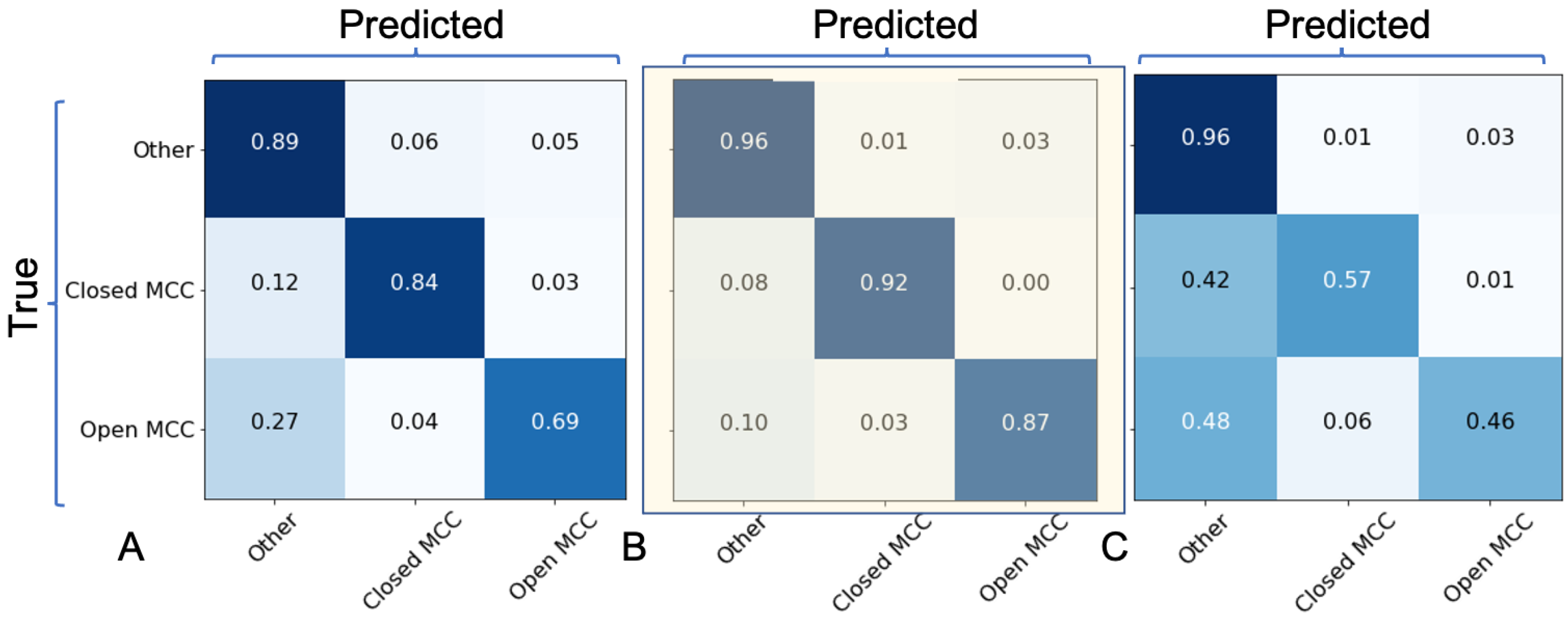
As detailed in the methodology section, our final model used the full Unet architecture, with the hyperparameters listed in Section 3.3, while training and predicting with three main classes, namely: (1) other, (2) closed MCC, and (3) open MCC. With the final setup, we trained the model twice: (1) on all randomly selected data patches (128 × 128) for the three classes (~9200 patches), hereafter referred to as the all-data model, and (2) only on patches that showed a majority (97% and above) of one class within the patch boundaries (~5050), hereafter referred to as the single-class model. Figure 5 presents the confusion matrix (CM) prediction accuracy on test patches not used in the model training for the two trained models. Figure 5A shows the all-data model predictions on patches containing more than one class per patch, and Figure 5B shows all-data model predictions on patches containing one class majority. Figure 5C shows the CM prediction results from a single-class-trained model used to predict patches containing multiple classes. The incentive of testing the prediction on patches having more than one class versus patches with one main class was to allow better comparison with current state-of-the-art models (i.e., [8]), which generate predictions of mostly uniform patches. As seen, when a patch contained one main class, the all-data trained model performed similarly to [8], with 92% vs. 94% for the closed MCC type, and 87% vs. 89% for the open MCC type, respectively. The fact that the open MCC type, when predicted in a multi-class patch, showed slightly lower accuracy rates seems to stem from the uncertainty in the boundary definition in instances where open MCCs are enclosed as POCs within a closed MCC deck. This was also shown recently by [10], where their pixel-by-pixel accuracy of POC predictions in MODIS imagery was much lower (not reported) compared with their accuracy based on an entire POC instance detection per image. The latter resulted in 86% POC prediction accuracy, very similar to ours. Conversely, in Figure 5C, we show that training a model on patches that contain mostly one class did not perform well when attempting to predict multi-class patches. This exercise revealed that the main errors we had were on the boundaries between multiple cloud classes. Hence, since the ground-truths on the boundaries are not well-defined because of the texture of the clouds that change smoothly, our overall model accuracy is actually higher than the reported confusion matrix accuracies.
Although we showed (Figure 5A,B) good detection rates for our test patches using the VIS model, we noted that when performing a prediction on the entire domain, closed and open MCC cloud coverage percentage decreased between 14:00 and 16:00 UTC. This is likely a result of the diminishing lighting available in or the VIS channel towards dusk. Hence, we explored this issue further and resolved it through the utilization of the IR-based model, as detailed in the next section.
4.2. MCC Semantic Segmentation—Comparison between VIS and IR Models
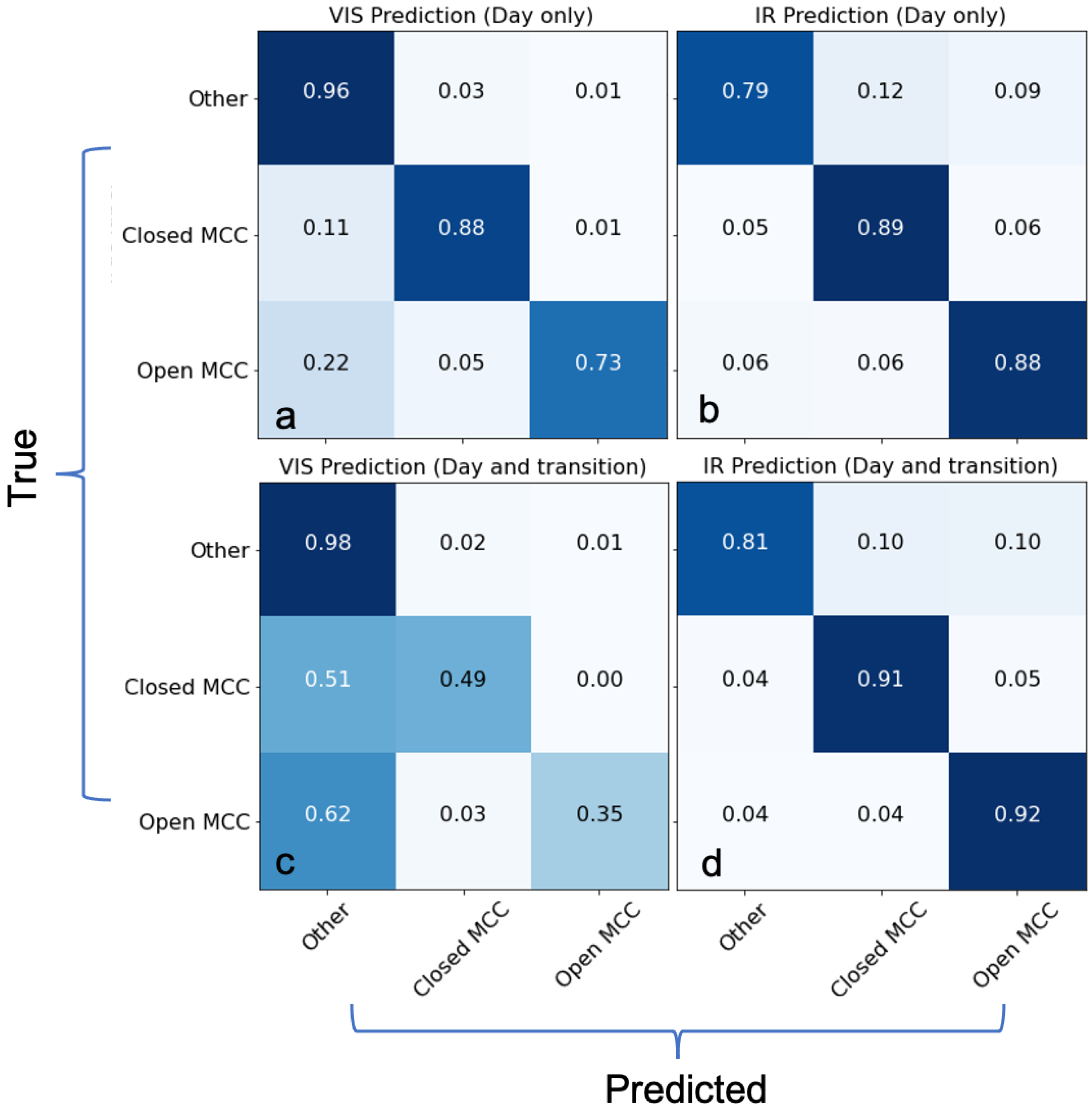
The IR-only model was trained with similar parameters as the VIS-only model, using the 10.8 mm scaled image channel as an input. In Figure 6 we show predictions from either the VIS-only model (a–c) and the IR-only model (d–f) for a test scene on 5 September 2017 at 10:00 UTC that was not used in the training. CM values for other, closed, and open MCC classes were 95%, 88%, and 73% for the VIS model, and 71%, 93%, and 95% for the IR model, respectively. The latter confirms the superiority of the IR model in better distinguishing between closed and open MCC cloud types, with the VIS-only model mostly confused between these two classes and the “other” class.
Figure 7 summarizes the comparison between the two models, with panels a and b showing VIS and IR confusion matrix results, respectively, for two full day-only scenes (at 10:00 and 12:00 UTC), and panels c and d show accumulated VIS and IR results, respectively, for four full test scenes (3639 × 3795 km2) including twilight times (where light is still available for visible imagery) at 08:00 and 16:00 UTC, which correspond to the local time at the domain location. These results demonstrate the better capability of the IR-only model to classify open MCC structure, as POCs or as larger patches, during both daytime and transition times, where the VIS model fails. As shown, the IR-only model seemed to suffer from low accuracy values for the “other” class type. This is likely a result of a mix of multiple classes into this one class with sufficiently different features as seen by the IR channel.
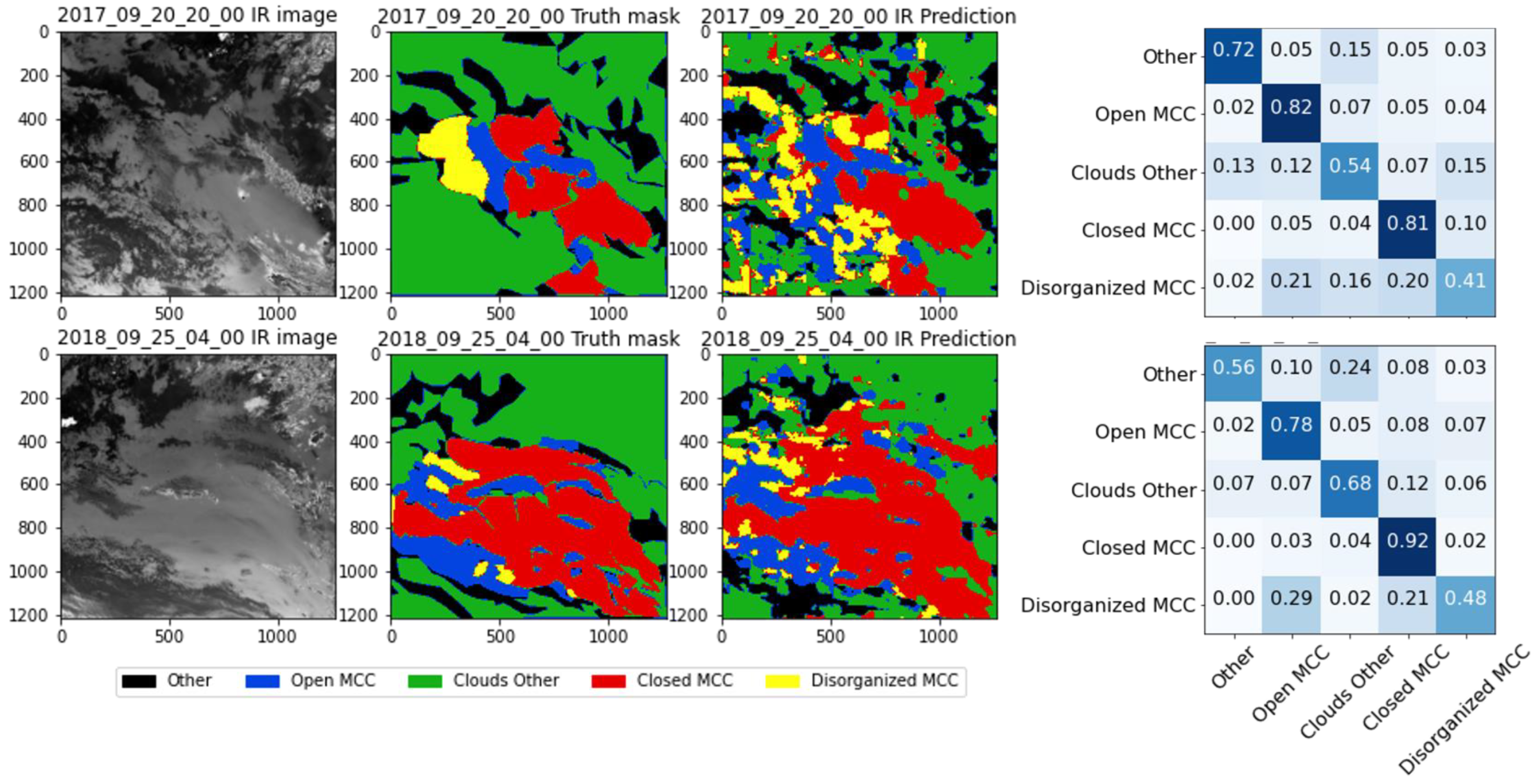
To investigate the capability of the IR-only model further, we trained an additional IR model, defining five classes to break down our “other” class back into disorganized and other types of clouds (mid- and high-level clouds), leaving the new “other” category to cover only clear ocean and land surfaces, as shown in Figure 8. Here, we see that the classes that exhibited low accuracy values were the disorganized and other clouds, while the open and closed classes exhibited high accuracy between 80 and 90% depending on the scenes. Additionally, it is worth mentioning that the truth masks, which were manually created, might have resulted in true-positive values to be low because of inconsistent truth labeling rather than because of real mis-classification by the model. This issue is evident in many other supervised machine learning applications, and especially ones for remote-sensing applications where intensive manual labeling can enhance predictability and accuracy but is very sparse due to its costly nature. Future solutions to this might include the development of an unsupervised classification scheme that can be used as a basis for a larger labeled dataset.
4.3. MCC Cloud Type Diurnal Variations and Seasonal Trends
In this section we present prediction results using our three-class IR-only CNN network architecture, for the period between August and October, covering 2016, 2017, and 2018 BB seasons that were also sampled by ORACLES.
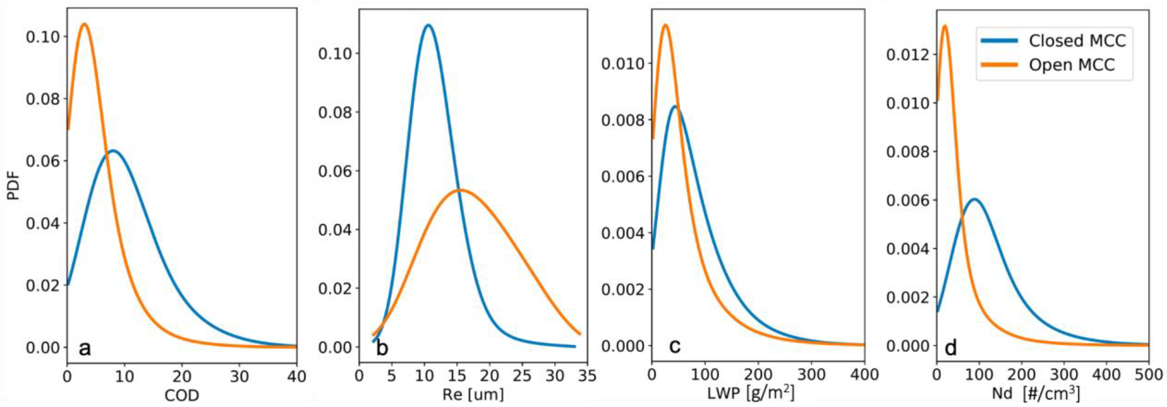
Figure 9 shows the probability distribution functions during the day (08:00–16:00 UTC) for the three BB seasons of closed and open MCC clouds for four cloud property variables available from the cloud property retrieval algorithms developed for MODIS [41,42] and applied on the SEVIRI dataset by the NASA Langley Cloud group (see data link in data the availability section). We show only daytime statistics because of the high uncertainty of the cloud property retrieval algorithm during the night. As seen, open MCC clouds showed larger effective radii (Re) and smaller cloud optical depths (COD) than closed MCC clouds, which is expected based on the fact that open MCC clouds are considered precipitating systems. This is also in accordance with [8,10], both analyzing several years of once-daily MODIS overpasses. As LWP is directly proportional to Re and COD in the MODIS retrieval algorithm, the LWP showed corresponding trends, especially dominated by COD. Additionally, as expected, cloud number concentration (Nd) was much higher for the closed MCC, as these are predominately non-precipitating systems.
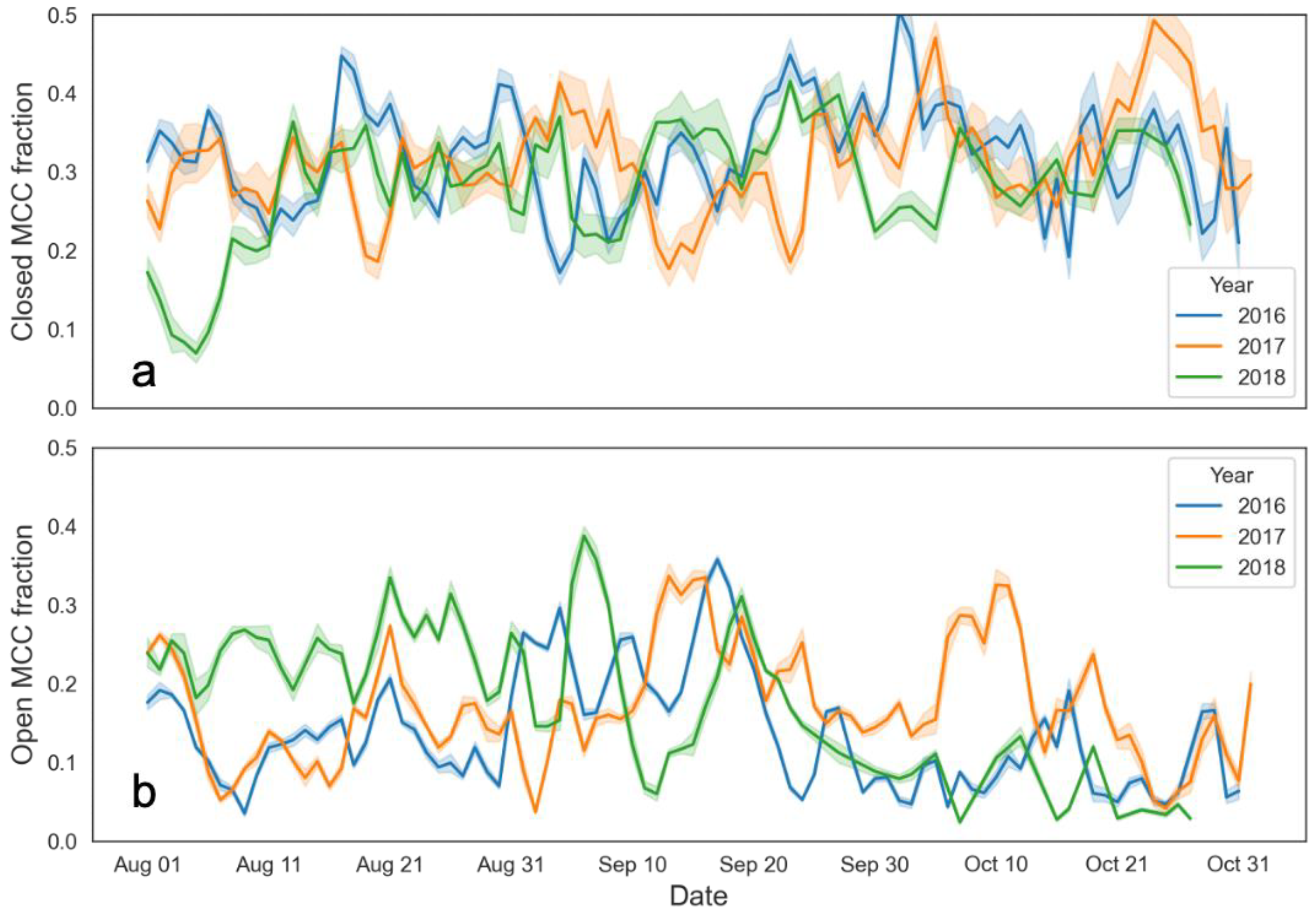
Figure 10 shows the seasonal variations based on half-hourly diurnal predictions for August through October for the three years corresponding with the ORACLES campaign (2016–2018). The closed MCC fraction (percentage cover of the research domain) ranged between 0.25 and 0.4, with some higher values spiking in mid-August 2016 and October 2017. Open MCC showed higher variability with an average of 15% coverage and peaks during August–September 2016, September and October 2017, and August 2018, with the latter corresponding to a low fraction in the closed MCC fraction (see Figure 10a).
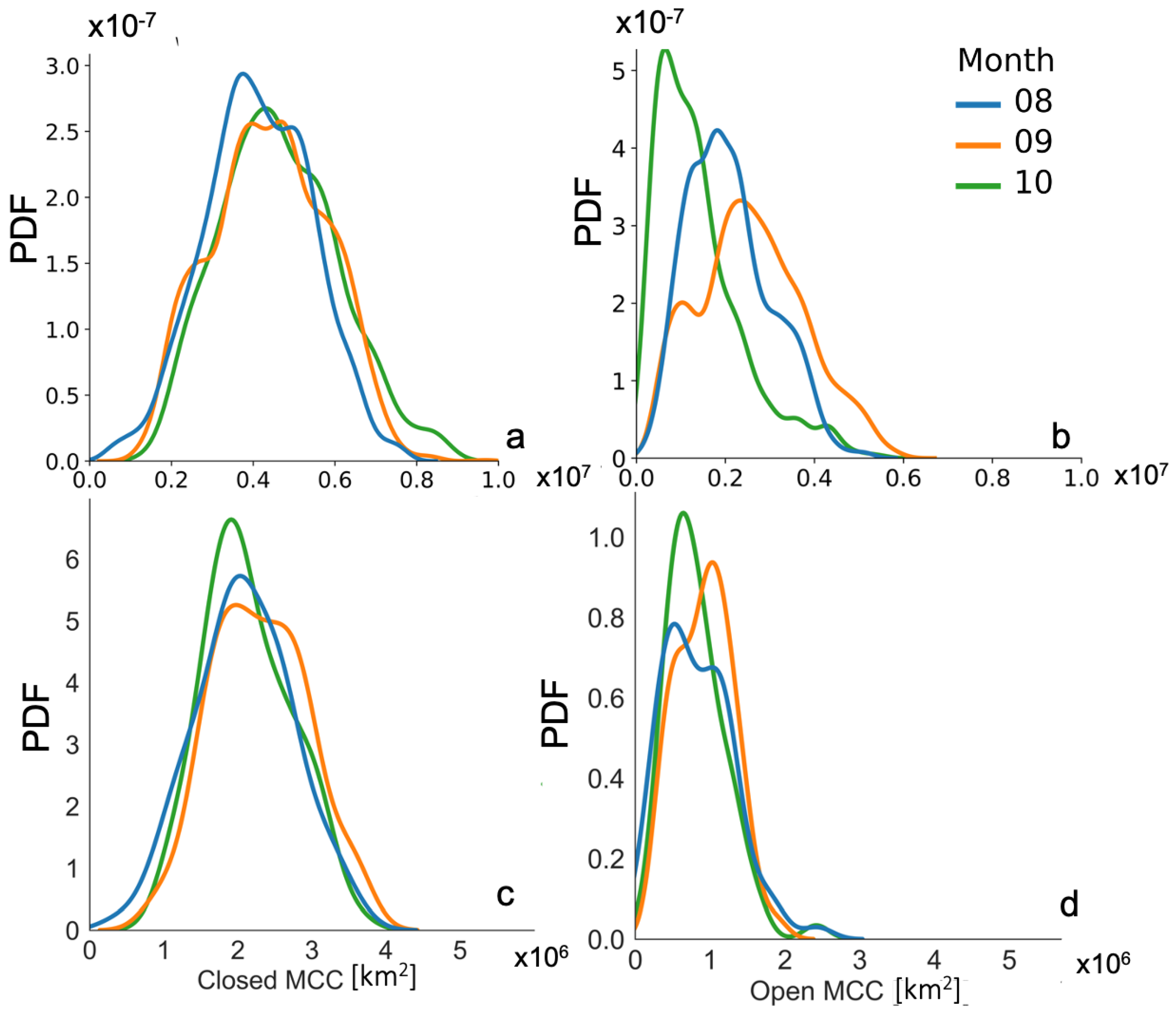
To validate and compare our results to available data from MODIS [8], we calculated the area coverage of closed and open MCC clouds classified by their method and compared it with our results. Since our algorithm assigns a class per each pixel, cloud area coverage was calculated by multiplying the domain area by the fractional cloud type amount, as the SEVIRI L1B product pixels are equidistant. Cloud type coverage area for Yuan et al. [8]’s product were calculated based on integrating the total area classified by the scheme (identifying a class per 128 × 128 km2 patch), where closed MCC uses the sum of both stratus and closed MCC (their classes being 0 and 1), and open MCC uses open MCC and clustered cumulus (their classes being 3 and 4) within the domain area. Although these two algorithms use two different approaches, we see that the cloud type area distributions (Figure 11) are remarkably similar. Specifically, while closed MCC area distributions were shown to be relatively constant for all three months (Figure 11a,c), open MCC showed differences among the three months, with October having a lower open MCC area coverage, following August and September (Figure 11b,d).
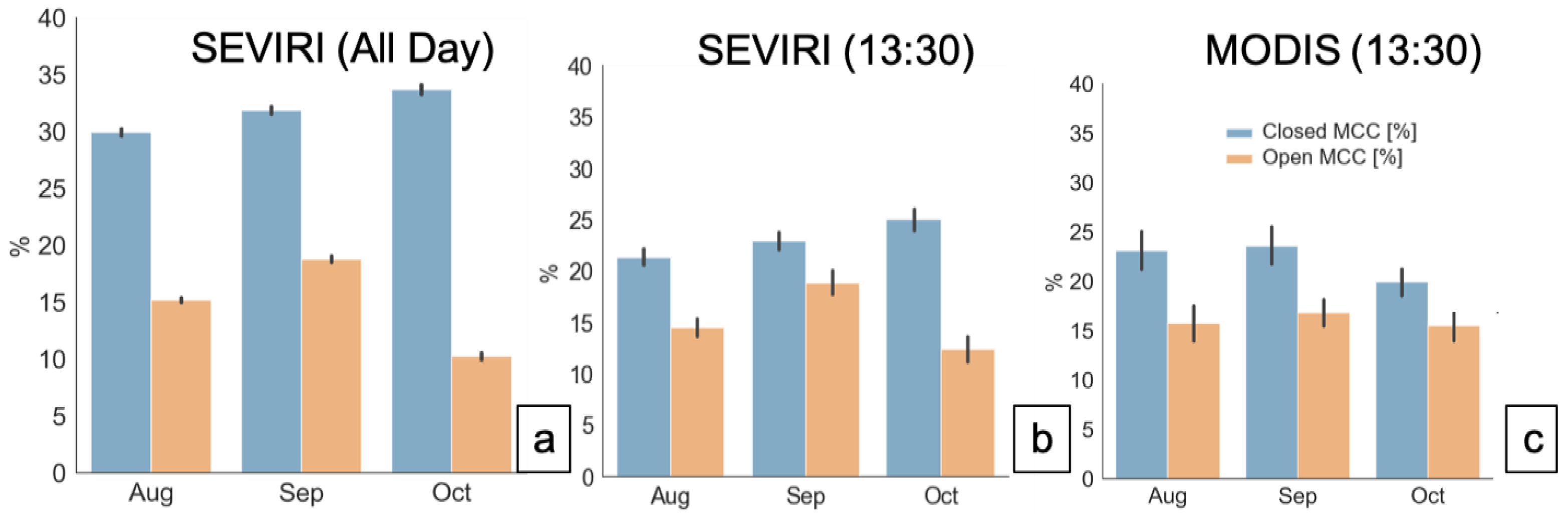
Furthermore, in Figure 12 we show the domain cloud coverage percentage comparisons. Figure 12a shows cloud type percentage means over the entire day (for 30 min. prediction intervals using SEVIRI data and the current methodology), while Figure 12b shows only daytime predictions that correspond to the MODIS Aqua overpass (at 13:30 local time). To compare with Yuan et al. [8], we used their closed and open MCC cloud area coverage (daily, over 2016–2018), calculated as detailed in Figure 11, divided by the total cloud area coverage given by their algorithm to obtain the domain area cloud coverage shown in Figure 12c. As seen, the results were fairly consistent with closed MCC coverage between 20 and 25% and open MCC at around 15% for both algorithms. The increase in closed MCC for the all-day SEVIRI data (Figure 12a) represents the increase in closed MCC during the night (see also Figure 13b).
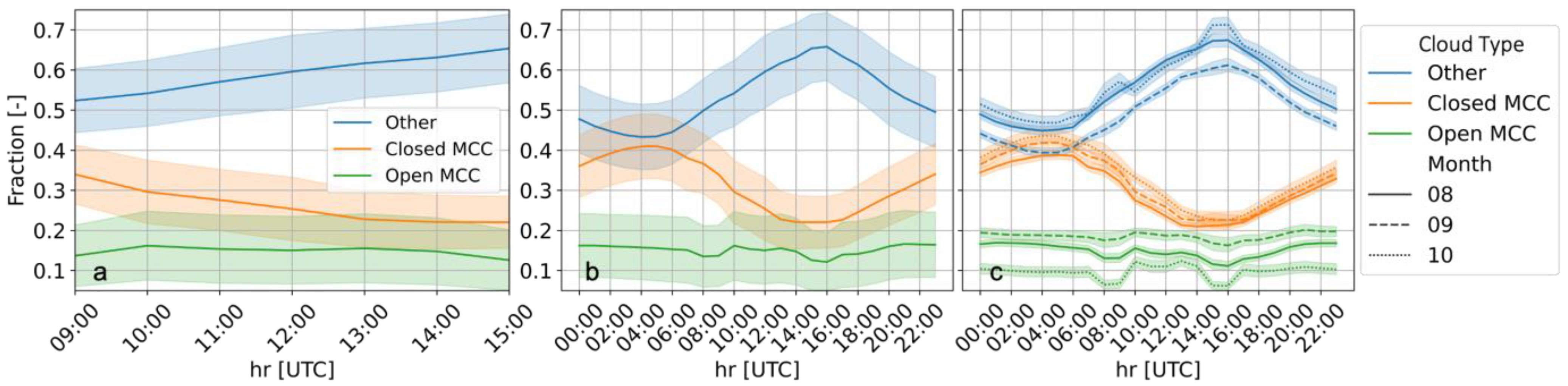
Figure 13 shows time-of-day variations of our class types, i.e., other, closed, and open MCC. Daytime variations were quite small, as depicted by Figure 13a, for both the closed and open MCC classes, and depict the need for a diurnal detection algorithm for better understanding of these clouds’ diurnal dynamics. While Figure 13a only shows the tail of the decrease in closed MCC from dawn onwards until the afternoon minimum, it allows one to derive the relatively steady behavior of both closed and open MCC during the day, a feature that was possible to extract due to the utilization of the IR model, which does not exhibit daytime illumination variability as its visible counterpart. As described by [43] and references therein, the diurnal cycle of marine BL clouds has a distinct but broad stratocumulus maximum during nighttime, which is also shown here (Figure 13b), occurring between 22:00 and 04:00 UTC, with a decrease after dawn. Applying our algorithm to MODIS day (13:30) and night (01:30) overpass scenes (not shown) also revealed a similar trend with nighttime closed MCC coverage, increasing to about 40%. We note that the decrease of closed MCC during the day (Figure 13b) was only slightly compensated by open MCC, mainly in the early and late afternoon, as is sometimes evident from the formation of POCs, which occupy only a small fraction of the domain. In contrast, closed MCC’s decrease often occurred with the “other” type increasing, the latter including both the disorganized MCC type but also other clouds and the open ocean. When inspecting the images visually, the decrease in closed MCC was initially compensated for by an increase in disorganized structures during the day, later (in the late afternoon) becoming either open or dissipating into clear sky scenes.
In Figure 13c we show the same diurnal variability as in Figure 13b, but separated into the main BB-dominated months, i.e., August through October. As seen, the diurnal variability of closed MCC was very small among these three months, and while the diurnal variability of open MCC was very small as well, the open MCC amount differed within these three months. Although others (e.g., [43,44]) have shown diurnal variability for MSC clouds from radar and microwave ground-based observations, as well as diurnal variability of LWP (i.e., morning and afternoon) from satellite observations (e.g., [45]), we note here that this is the first time that the diurnal variability of MCC cloud types was described from high-temporal-resolution satellite observations. Reasons for the differences in seasonal variability of open MCC within the investigated period might include the fact that meteorological conditions, as well as fire conditions and aerosol amount and composition (as described by e.g., [46]), were different between the three months. However, the relationships between aerosol amount and type and cloud properties are beyond the scope of this work and are developed in a companion paper (in prep.). A decrease in POC from August through October over the SEA cloud deck was also observed by [10] using 13-year daytime MODIS climatology, which supports our results shown here.
4.4. Application of IR Model MCC Classification on GOES-ABI
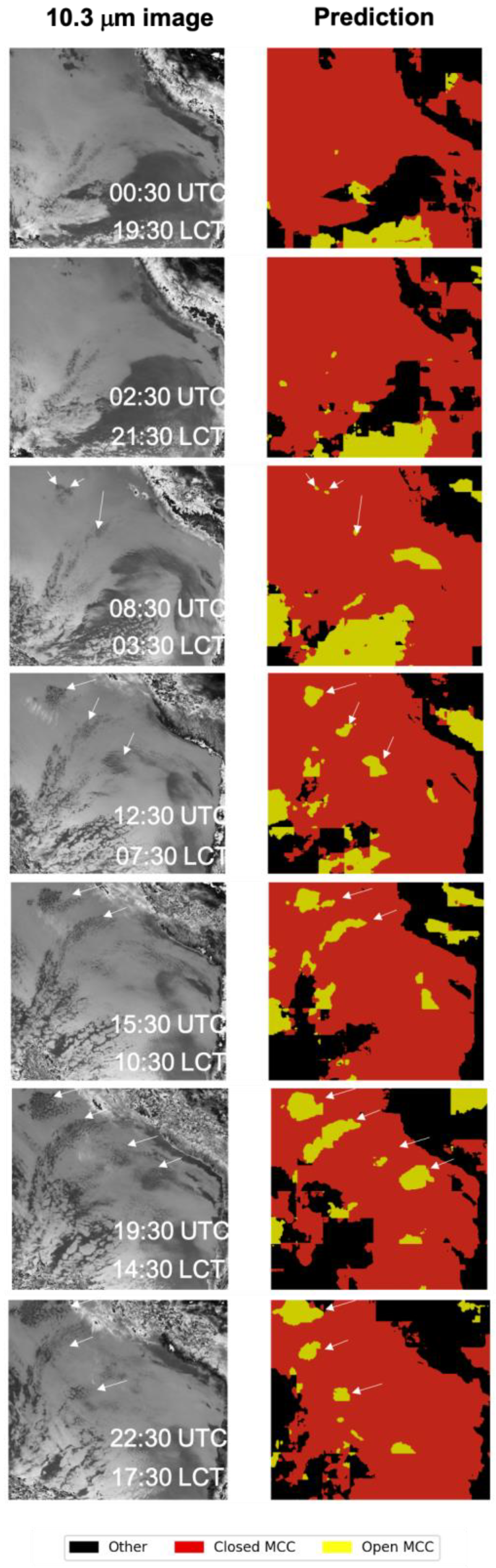
To test the applicability of our algorithm towards a global product, we used our IR-only model that was trained on SEVIRI images (as detailed above) to predict closed and open MCC cloud types from GOES-16. This was carried out for the Peruvian stratocumulus semi-permanent cloud deck over the SEP (South-East Pacific) domain covering the region between 10–30°S and 70–90°W. The two main differences among the SEVIRI and the GOES-16 are the spectral band maximum of the IR input channel (10.3 mm in GOES compared with 10.8 mm in SEVIRI) and the slightly higher spatial resolution (2 km compared with 3 km) ground FOV (field-of-view) per pixel. Despite these differences, we did not make any adjustments to our model prior to prediction and the only pre-processing performed on the input was the scaling according to Equation (1). Figure 14 shows an example of prediction for 1 October 2018 over the SEP domain using the GOES-16 10.3 mm channel as input, with several distinct time-stamps. As seen, closed MCC cover was dominant during the night (upper three rows), while the non-bounded open cells seemed to prevail during the night and decrease at sunrise (07:30 LT), and POCs started to grow and aggregate from before sunrise and peaked in the afternoon (14:30 LT). The open MCCs observed at the bottom parts of the image were converted to structures resembling more disorganized MCCs and hence are marked by black (i.e., the “other” class, which combines several cloud and background types). Additional misclassification can occur since GOES has different resolutions than the training dataset; thus, it is possible that if the clouds are too broken in the open cell (e.g., clustered cumulus), they will be classified as “other”.
Nevertheless, although we did not generate ground truth for this region, we see that our model was able to capture the formation and dissipation of open MCCs and the expansion of the closed MCC regions as the night progressed.
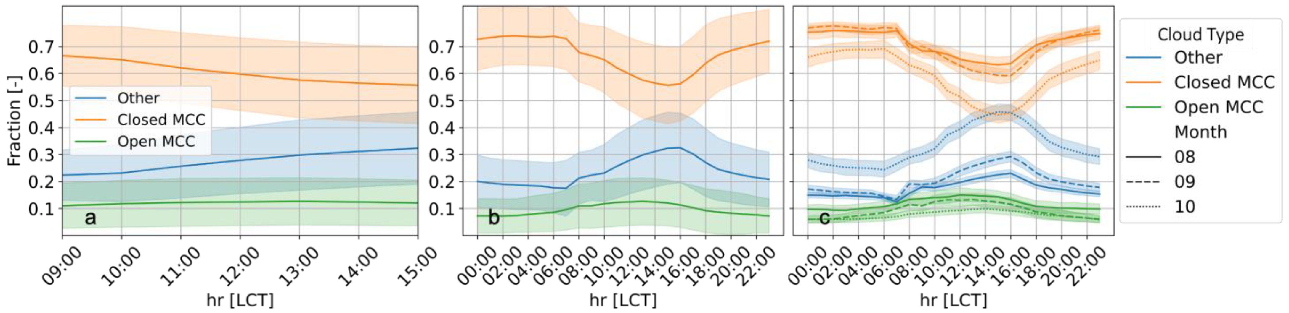
Figure 15 further shows daytime and diurnal plots, similar to Figure 13, but for the SEP region. Data were available only for Aug–Oct for 2018. As shown, daytime and diurnal trends followed similar behavior for both the SEA and SEP regions, with minimal changes during daytime hours and a decrease in the closed MCC coverage later in the day, peaking broadly during the night. Nevertheless, there was a small trend showing open cells increased during the day, between 10:00 and 14:00 local time (evident also in Figure 14), and indeed, Wood et al. [47] showed that POCs over the SEP preferentially form during early morning hours when precipitation maximizes, which partially explains our observation of this daytime maximum. Another interesting difference is the percentage coverage among cloud types over the SEP, where closed MCCs dominated the scene for the entire season (slightly less in October) and exhibited much larger fractions when compared to their counterparts in the SEA region. Since closed MCCs have been associated with higher lower tropospheric stability (LTS), e.g., [2], we postulate that the higher monthly mean LTS calculated from ERA-5 reanalysis over the SEP (22–24 over the entire domain) during these months compared with the SEA (19–20 over the domain) and the larger spatial spread of this stability over the SEP domain is the main reason for this. Finally, open MCC featured a similar trend to that observed in other investigations (e.g., [10]), i.e., a decrease in open MCC coverage from August through October.
5. Discussion
In this work, we developed a CNN-based model for semantic segmentation of MCC cloud types. These clouds are common over vast areas over the Earth’s oceans and exist mostly as semi-permanent cloud decks, specifically off the coast of Namibia, over the SEA, off the coast of Chile, over the SEP, and off the coast of California. Their persistence and radiatively important properties play a large role in the Earth’s radiative budget, while also causing confounding results in global models aiming at their accurate predictions. While heavily investigated using multiple observational (ground-based, in-situ, satellite) and modeling tools (e.g., [2,5,43,47] and references therein), current remote-sensing schemes that perform MCC classification have been developed for day-only observations, e.g., Wood and Hartmann [4] and Yuan et al. [8], for MODIS, and in addition, only predict the patch type (either 256 × 256 km2 or 128 × 128 km2, respectively). Newer algorithms such that of Watson-Parris et al. [10], which was developed using a semantically segmented CNN-based model, only predict a certain type of cloud, which are the open-cell pockets enclosed within the closed-cell deck, and do so only for daytime scenes. Herein, we expanded and developed a semantically segmented CNN-based algorithm classifying both closed and open MCC cells in the broad sense, where not only enclosed open cells are classified, but a wider variety, which also allows tracking the closed-to-open cell transitions over larger areas. In addition, our algorithm classifies IR images, which allows generating both day and night predictions for an improved understanding of these unique clouds’ diurnal cycles and their dependency on meteorological and environmental variables. This is the first time that MCC cloud types could be classified from space during both day and night, and since the diurnal cycle of mesoscale organizations has barely been studied before, our work sheds new light on that. Indeed, recently Zhang and Zuidema [43] showed the diurnal cycle of low-level clouds over Ascension Island, but this was based on cloud classes observed and classified from a single ground-based location, noting their instantaneous definition (e.g., cumulus, stratocumulus, etc.), which is hard to extrapolate regionally.
When testing visible and infrared images as inputs to our algorithm, we realized that visible images when used during transition times of day (early morning and late afternoon) did not yield good prediction results due to illumination differences. In contrast, we found that the IR-only based model was capable of accurately predicting the almost-constant coverage of both closed and open MCC clouds during the day, while also allowing the probing of their diurnal variability under different conditions. The latter was used to show that during October, a month with a relatively low BB amount, open MCC diurnal variation was more distinct than in months with higher BB amounts such as August and September. Furthermore, and concurrent with previous observations, the amount of open MCC derived by our algorithm was shown to be higher during August and September than October, with a relatively stable coverage amount by the closed MCC cloud type over the SEA domain. Diurnal variability derived from our algorithm has corroborated ground-based observations, noticing the broad closed MCC peak during nighttime and its dissipation during the day.
To validate our algorithm further, we compared various closed and open MCC cloud property distributions with the available literature and found that during the day our results corresponded well with available distributions for Re and COD, where open MCC Re was higher and COD was lower when compared with closed MCC. In addition, we also observed an increased cloud number concentration in the closed MCC cloud types, as expected.
When comparing cloud type area coverage between the current work and [8], we found similar trends wherein closed MCC area did not change much during the BB season and open MCC decreased in October. In addition, when comparing cloud type cover (in percentage) over the SEA domain, our results and the algorithm developed by [8] yielded similar results, with closed MCC occupying about 25–30% of the domain and open MCC 15–20% during the day.
In our attempt to generalize the prediction model on a different satellite platform, we applied our IR-only model trained on SEVIRI imagery over the SEA domain to GOES-16 new-generation imagery over the SEP domain. Here, we showed good prediction results, coherent with the SEA results when inspected visually. In addition, when examining the diurnal variation over August–October of 2018, we found similar behavior to the SEA domain, with a more distinct increase in open MCC during the day and a decrease from August through October, while closed MCC dominated this domain, most likely because of higher regional lower tropospheric stability.
Nevertheless, to further test and quantify our algorithm globally, we will need to generate a larger set of truth labels, which will make the algorithm more robust, especially if we also want to predict disorganized MCCs, which are more subjective to define when only using visual imagery. Additional effort and verification are needed to compare predictions generated for different spatial resolution inputs, as briefly demonstrated here.
Future applications to use this algorithm are ongoing and we are currently utilizing the method developed herein, collocated with fine temporal and spatial resolution airborne in situ data, to study closed and open MCC cloud adjustments over the SEA during the BB season.
Author Contributions
Paper conceptualization, funding acquisition, methodology, data curation, formal analysis, visualization, software and writing original draft, M.S.R.; software, D.N.; data curation formal analysis and visualization, H.C.; writing—review and editing, M.S.R., D.N., H.C., R.W. and Z.Z. All authors have read and agreed to the published version of the manuscript.
Funding
This research was funded by the NASA Atmospheric Composition and Modeling program (ACMAP), through the NNH18ZDA001N grant.
Data Availability Statement
SEVIRI multi-channel georectified and calibrated files were downloaded from the University of Lille ftp website: ftp.icare.univ-lille1.fr (accessed on 1 November 2021), using /SPACEBORNE/GEO/MSG+0000/L1_B for SEVIRI data over the SEA, and /SPACEBORNE/GEO/GOESNG-0750/L1_B/ for GOES data over the SEP. SEVIRI processed cloud products, generated by the NASA Langley center were downloaded from: https://cloud1.arc.nasa.gov/oracles/data/ (accessed on 1 November 2021), Level 2 MCC cloud type product from MODIS generated by [8] were downloaded from here: https://disc.gsfc.nasa.gov/datasets/MYD_L2_MPLCT_001/summary?keywords=MYD_L2_MPLCT_001 (accessed on 1 November 2021). Software codes and training data can be found under: https://github.com/DavidHuji/clouds_segmentation (accessed on 1 November 2021).
Acknowledgments
We would like to thank to Jerome Reidi for his contribution to the availability and interpretation of the L1B SEVIRI dataset, and Douglas Spangenberg, for his assistance with the SEVIRI cloud products processing for the ORACLES campaign.
Conflicts of Interest
The authors declare no conflict of interest. The funders had no role in the design of the study; in the collection, analyses, or interpretation of data; in the writing of the manuscript; or in the decision to publish the results.
References
- Muhlbauer, A.; McCoy, I.L.; Wood, R. Climatology of stratocumulus cloud morphologies: Microphysical properties and radiative effects. Atmos. Chem. Phys. 2014, 14, 6695–6716. [Google Scholar] [CrossRef] [Green Version]
- McCoy, I.L.; Wood, R.; Fletcher, J.K. Identifying Meteorological Controls on Open and Closed Mesoscale Cellular Convection Associated with Marine Cold Air Outbreaks. JGR Atmos. 2017, 122, 11678–11702. [Google Scholar] [CrossRef] [Green Version]
- Gufan, A.; Lehahn, Y.; Fredj, E.; Price, C.; Kurchin, R.; Koren, I. Segmentation and Tracking of Marine Cellular Clouds observed by Geostationary Satellites. Int. J. Remote Sens. 2016, 37, 1055–1068. [Google Scholar] [CrossRef]
- Wood, R.; Hartmann, D.L. Spatial Variability of Liquid Water Path in Marine Low Cloud: The Importance of Mesoscale Cellular Convection. J. Clim. 2006, 19, 1748–1764. [Google Scholar] [CrossRef]
- Wood, R.; Bretherton, C.S.; Leon, D.; Clarke, A.D.; Zuidema, P.; Allen, G.; Coe, H. An aircraft case study of the spatial transition from closed to open mesoscale cellular convection over the Southeast Pacific. Atmos. Chem. Phys. 2011, 11, 2341–2370. [Google Scholar] [CrossRef] [Green Version]
- Redemann, J.; Wood, R.; Zuidema, P.; Doherty, S.J.; Luna, B.; LeBlanc, S.E.; Diamond, M.S.; Shinozuka, Y.; Chang, I.Y.; Ueyama, R.; et al. An overview of the ORACLES (ObseRvations of Aerosols above CLouds and their intEractionS) project: Aerosol–cloud–radiation interactions in the southeast Atlantic basin. Atmos. Chem. Phys. 2021, 21, 1507–1563. [Google Scholar] [CrossRef]
- Chang, I.; Christopher, S.A. Identifying Absorbing Aerosols Above Clouds from the Spinning Enhanced Visible and Infrared Imager Coupled with NASA A-Train Multiple Sensors. IEEE Trans. Geosci. Remote Sens. 2016, 54, 3163–3173. [Google Scholar] [CrossRef]
- Yuan, T.; Song, H.; Wood, R.; Mohrmann, J.; Meyer, K.; Oreopoulos, L.; Platnick, S. Applying deep learning to NASA MODIS data to create a community record of marine low-cloud mesoscale morphology. Atmos. Meas. Tech. 2020, 13, 6989–6997. [Google Scholar] [CrossRef]
- Vallet, A.; Sakamoto, H. A Multi-Label Convolutional Neural Network for Automatic Image Annotation. J. Inf. Process. 2015, 23, 767–775. [Google Scholar] [CrossRef] [Green Version]
- Watson-Parris, D.; Sutherland, S.A.; Christensen, M.W.; Eastman, R.; Stier, P. A Large-Scale Analysis of Pockets of Open Cells and Their Radiative Impact. Geophys. Res. Lett. 2021, 48, e2020GL092213. [Google Scholar] [CrossRef]
- Segal-Rozenhaimer, M.; Li, A.; Das, K.; Chirayath, V. Cloud detection algorithm for multi-modal satellite imagery using convolutional neural-networks (CNN). Remote Sens. Environ. 2020, 237, 111446. [Google Scholar] [CrossRef]
- Li, A.S.; Chirayath, V.; Segal-Rozenhaimer, M.; Torres-Perez, J.L.; van den Bergh, J. NASA NeMO-Net’s Convolutional Neural Network: Mapping Marine Habitats with Spectrally Heterogeneous Remote Sensing Imagery. IEEE J. Sel. Top. Appl. Earth Obs. Remote Sens. 2020, 13, 5115–5133. [Google Scholar] [CrossRef]
- Sakaeda, N.; Wood, R.; Rasch, P.J. Direct and semidirect aerosol effects of southern African biomass burning aerosol. J. Geophys. Res. 2011, 116, D12205. [Google Scholar] [CrossRef]
- Zuidema, P.; Redemann, J.; Haywood, J.; Wood, R.; Piketh, S.; Hipondoka, M.; Formenti, P. Smoke and Clouds above the Southeast Atlantic: Upcoming Field Campaigns Probe Absorbing Aerosol’s Impact on Climate. Bull. Am. Meteorol. Soc. 2016, 97, 1131–1135. [Google Scholar] [CrossRef] [Green Version]
- Swap, R.; Garstang, M.; Macko, S.A.; Tyson, P.D.; Maenhaut, W.; Artaxo, P.; Kållberg, P.; Talbot, R. The long-range transport of southern African aerosols to the tropical South Atlantic. J. Geophys. Res. 1996, 101, 23777–23791. [Google Scholar] [CrossRef]
- Painemal, D.; Kato, S.; Minnis, P. Boundary layer regulation in the southeast Atlantic cloud microphysics during the biomass burning season as seen by the A-train satellite constellation. J. Geophys. Res. Atmos. 2014, 119, 11288–11302. [Google Scholar] [CrossRef]
- Zhang, Z.; Meyer, K.; Yu, H.; Platnick, S.; Colarco, P.; Liu, Z.; Oreopoulos, L. Shortwave direct radiative effects of above-cloud aerosols over global oceans derived from 8 years of CALIOP and MODIS observations. Atmos. Chem. Phys. 2016, 16, 2877–2900. [Google Scholar] [CrossRef] [Green Version]
- Haywood, J.M.; Abel, S.J.; Barrett, P.A.; Bellouin, N.; Blyth, A.; Bower, K.N.; Brooks, M.; Carslaw, K.; Che, H.; Coe, H.; et al. The CLoud–Aerosol–Radiation Interaction and Forcing: Year 2017 (CLARIFY-2017) measurement campaign. Atmos. Chem. Phys. 2021, 21, 1049–1084. [Google Scholar] [CrossRef]
- Zuidema, P.; Chiu, C.; Fairall, C.; Ghan, S.; Kollias, P.; McFarguhar, G.; Mechem, D.; Romps, D.; Wong, H.; Yuter, S.; et al. Layered Atlantic Smoke Interactions with Clouds (LASIC) Science Plan; DOE Office of Science Atmospheric Radiation Measurement (ARM) Program (United States): Washington, DC, USA, 2015; p. 49.
- Wilcox, E.M. Stratocumulus cloud thickening beneath layers of absorbing smoke aerosol. Atmos. Chem. Phys. 2010, 10, 11769–11777. [Google Scholar] [CrossRef] [Green Version]
- Wilcox, E.M. Direct and semi-direct radiative forcing of smoke aerosols over clouds. Atmos. Chem. Phys. 2012, 12, 139–149. [Google Scholar] [CrossRef] [Green Version]
- Lu, Z.; Liu, X.; Zhang, Z.; Zhao, C.; Meyer, K.; Rajapakshe, C.; Wu, C.; Yang, Z.; Penner, J.E. Biomass smoke from southern Africa can significantly enhance the brightness of stratocumulus over the southeastern Atlantic Ocean. Proc. Natl. Acad. Sci. USA 2018, 115, 2924–2929. [Google Scholar] [CrossRef] [PubMed] [Green Version]
- Che, H.; Stier, P.; Gordon, H.; Watson-Parris, D.; Deaconu, L. Cloud adjustments dominate the overall negative aerosol radiative effects of biomass burning aerosols in UKESM1 climate model simulations over the south-eastern Atlantic. Atmos. Chem. Phys. 2021, 21, 17–33. [Google Scholar] [CrossRef]
- Diamond, M.S.; Saide, P.E.; Zuidema, P.; Ackerman, A.S.; Doherty, S.J.; Fridlind, A.M.; Gordon, H.; Howes, C.; Kazil, J.; Yamaguchi, T.; et al. Cloud adjustments from large-scale smoke–circulation interactions strongly modulate the southeastern Atlantic stratocumulus-to-cumulus transition. Atmos. Chem. Phys. 2022, 22, 12113–12151. [Google Scholar] [CrossRef]
- LeCun, Y.; Bengio, Y.; Hinton, G. Deep learning. Nature 2015, 521, 436–444. [Google Scholar] [CrossRef]
- Zhong, Y.; Fei, F.; Liu, Y.; Zhao, B.; Jiao, H.; Zhang, L. SatCNN: Satellite image dataset classification using agile convolutional neural networks. Remote Sens. Lett. 2017, 8, 136–145. [Google Scholar] [CrossRef]
- Maggiori, E.; Tarabalka, Y.; Charpiat, G.; Alliez, P. Convolutional Neural Networks for Large-Scale Remote-Sensing Image Classification. IEEE Trans. Geosci. Remote Sens. 2017, 55, 645–657. [Google Scholar] [CrossRef] [Green Version]
- Pešek, O.; Segal-Rozenhaimer, M.; Karnieli, A. Using Convolutional Neural Networks for Cloud Detection on VENμS Images over Multiple Land-Cover Types. Remote Sens. 2022, 14, 5210. [Google Scholar] [CrossRef]
- Long, J.; Shelhamer, E.; Darrell, T. Fully Convolutional Networks for Semantic Segmentation. In Proceedings of the IEEE Conference on Computer Vision and Pattern Recognition, Boston, MA, USA, 7–12 June 2015; pp. 3431–3440. [Google Scholar]
- Simonyan, K.; Zisserman, A. Very Deep Convolutional Networks for Large-Scale Image Recognition. arXiv 2015. [Google Scholar] [CrossRef]
- He, K.; Zhang, X.; Ren, S.; Sun, J. Deep Residual Learning for Image Recognition. In Proceedings of the 2016 IEEE Conference on Computer Vision and Pattern Recognition (CVPR), Las Vegas, NV, USA, 27–30 June 2016; IEEE: New York, NY, USA; pp. 770–778. [Google Scholar]
- Chen, L.-C.; Papandreou, G.; Kokkinos, I.; Murphy, K.; Yuille, A.L. DeepLab: Semantic Image Segmentation with Deep Convolutional Nets, Atrous Convolution, and Fully Connected CRFs. IEEE Trans. Pattern Anal. Mach. Intell. 2018, 40, 834–848. [Google Scholar] [CrossRef] [Green Version]
- Ronneberger, O.; Fischer, P.; Brox, T. U-Net: Convolutional Networks for Biomedical Image Segmentation. In Medical Image Computing and Computer-Assisted Intervention—MICCAI 2015; Navab, N., Hornegger, J., Wells, W.M., Frangi, A.F., Eds.; Lecture Notes in Computer Science; Springer International Publishing: Cham, Switzerland, 2015; Volume 9351, pp. 234–241. ISBN 978-3-319-24573-7. [Google Scholar]
- Badrinarayanan, V.; Kendall, A.; Cipolla, R. SegNet: A Deep Convolutional Encoder-Decoder Architecture for Image Segmentation. IEEE Trans. Pattern Anal. Mach. Intell. 2017, 39, 2481–2495. [Google Scholar] [CrossRef]
- Wada, K. Labelme: Image Polygonal Annotation with Python; MIT Computer Science and Artificial Intelligence Laboratory (CSAIL): Cambridge, MA, USA, 2016; Available online: https://github.com/wkentaro/labelme (accessed on 1 October 2021).
- Buda, M.; Saha, A.; Mazurowski, M.A. Association of genomic subtypes of lower-grade gliomas with shape features automatically extracted by a deep learning algorithm. Comput. Biol. Med. 2019, 109, 218–225. [Google Scholar] [CrossRef] [Green Version]
- Lin, T.-Y.; Goyal, P.; Girshick, R.; He, K.; Dollar, P. Focal Loss for Dense Object Detection. In Proceedings of the IEEE International Conference on Computer Vision, Venice, Italy, 22–29 October 2017; pp. 2980–2988. [Google Scholar]
- Kingma, D.P.; Ba, J. Adam: A Method for Stochastic Optimization. arXiv 2017. [Google Scholar] [CrossRef]
- Glorot, X.; Bengio, Y. Understanding the difficulty of training deep feedforward neural networks. In Proceedings of the Thirteenth International Conference on Artificial Intelligence and Statistics, JMLR Workshop and Conference Proceedings, Sardinia, Italy, 13–15 May 2010; pp. 249–256. [Google Scholar]
- Jean, S.; Soille, P. Mathematical Morphology and Its Applications to Image Processing; Springer Science & Business Media: Berlin/Heidelberg, Germany, 2012. [Google Scholar]
- Minnis, P.; Sun-Mack, S.; Young, D.F.; Heck, P.W.; Garber, D.P.; Chen, Y.; Spangenberg, D.A.; Arduini, R.F.; Trepte, Q.Z.; Smith, W.L.; et al. CERES Edition-2 Cloud Property Retrievals Using TRMM VIRS and Terra and Aqua MODIS Data—Part I: Algorithms. IEEE Trans. Geosci. Remote Sens. 2011, 49, 4374–4400. [Google Scholar] [CrossRef]
- Yost, C.R.; Minnis, P.; Sun-Mack, S.; Chen, Y.; Smith, W.L. CERES MODIS Cloud Product Retrievals for Edition 4—Part II: Comparisons to CloudSat and CALIPSO. IEEE Trans. Geosci. Remote Sens. 2021, 59, 3695–3724. [Google Scholar] [CrossRef]
- Zhang, J.; Zuidema, P. The diurnal cycle of the smoky marine boundary layer observed during August in the remote southeast Atlantic. Atmos. Chem. Phys. 2019, 19, 14493–14516. [Google Scholar] [CrossRef] [Green Version]
- Eastman, R.; Warren, S.G. Diurnal Cycles of Cumulus, Cumulonimbus, Stratus, Stratocumulus, and Fog from Surface Observations over Land and Ocean. J. Clim. 2014, 27, 2386–2404. [Google Scholar] [CrossRef] [Green Version]
- Wood, R.; Bretherton, C.S.; Hartmann, D.L. Diurnal cycle of liquid water path over the subtropical and tropical oceans: DIURNAL CYCLE of LIQUID WATER PATH. Geophys. Res. Lett. 2002, 29, 7-1–7-4. [Google Scholar] [CrossRef] [Green Version]
- Che, H.; Segal-Rozenhaimer, M.; Zhang, L.; Dang, C.; Zuidema, P.; Sedlacek III, A.J.; Zhang, X.; Flynn, C. Seasonal variations in fire conditions are important drivers in the trend of aerosol optical properties over the south-eastern Atlantic. Atmos. Chem. Phys. 2022, 22, 8767–8785. [Google Scholar] [CrossRef]
- Wood, R.; Comstock, K.K.; Bretherton, C.S.; Cornish, C.; Tomlinson, J.; Collins, D.R.; Fairall, C. Open cellular structure in marine stratocumulus sheets. J. Geophys. Res. 2008, 113, D12207. [Google Scholar] [CrossRef] [Green Version]
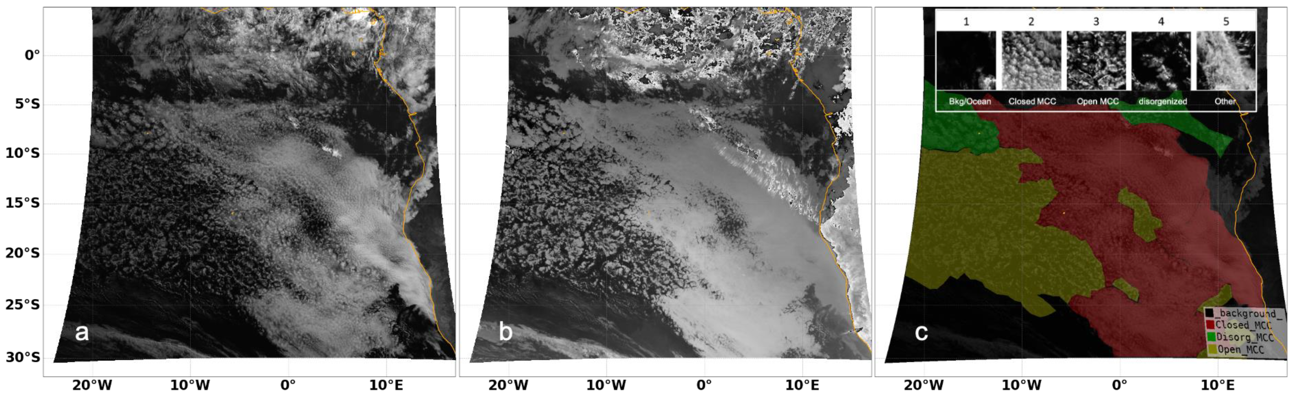
Figure 1.
(a) SEVIRI VIS channel (0.6 mm), (b) IR channel (10.8 mm), and (c) MCC cloud type regions (closed, open, and disorganized) as labeled for the training process overlying the visible image. The image is from 20 August 2016, 09:00 UTC, showing the research area and training domain over the SEA Ocean. The insert in (c) shows examples of the different cloud types recognized within the research domain, with type (Bkg/ocean) and other (other cloud types, not MCC) lumped together as background/other types in the final training process. MCC cloud types and their selection for the model training are further detailed in the Section 3.

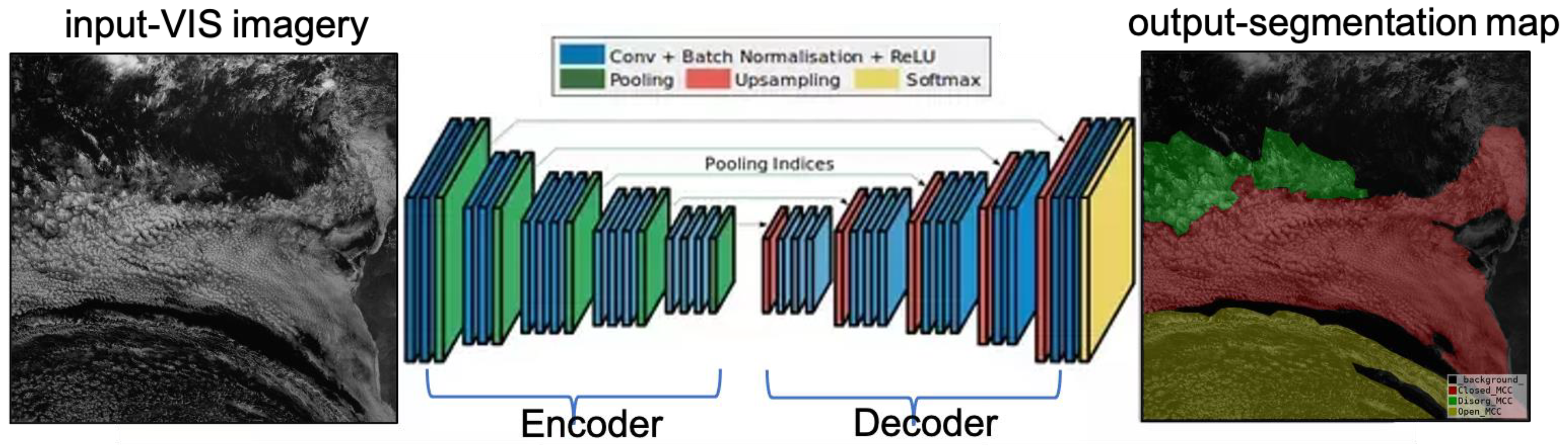
Figure 2.
A general scheme of a fully convolutional network (adapted from [34]) that generates a semantic segmentation cloud classification map with an imagery input layer (of VIS channel in this case). The encoder part includes a series of convolutions, batch normalizations, and activation functions, each to extract spatial features diminishing the original imagery dimensions. The decoder part includes convolutions and upsampling operations, also drawing from various encoder layer outputs, to re-generate the original image dimensions. The final output layer is a multi-class map (with dimensions similar to the input image) generated by a multi-class SOFTMAX probabilistic output function.

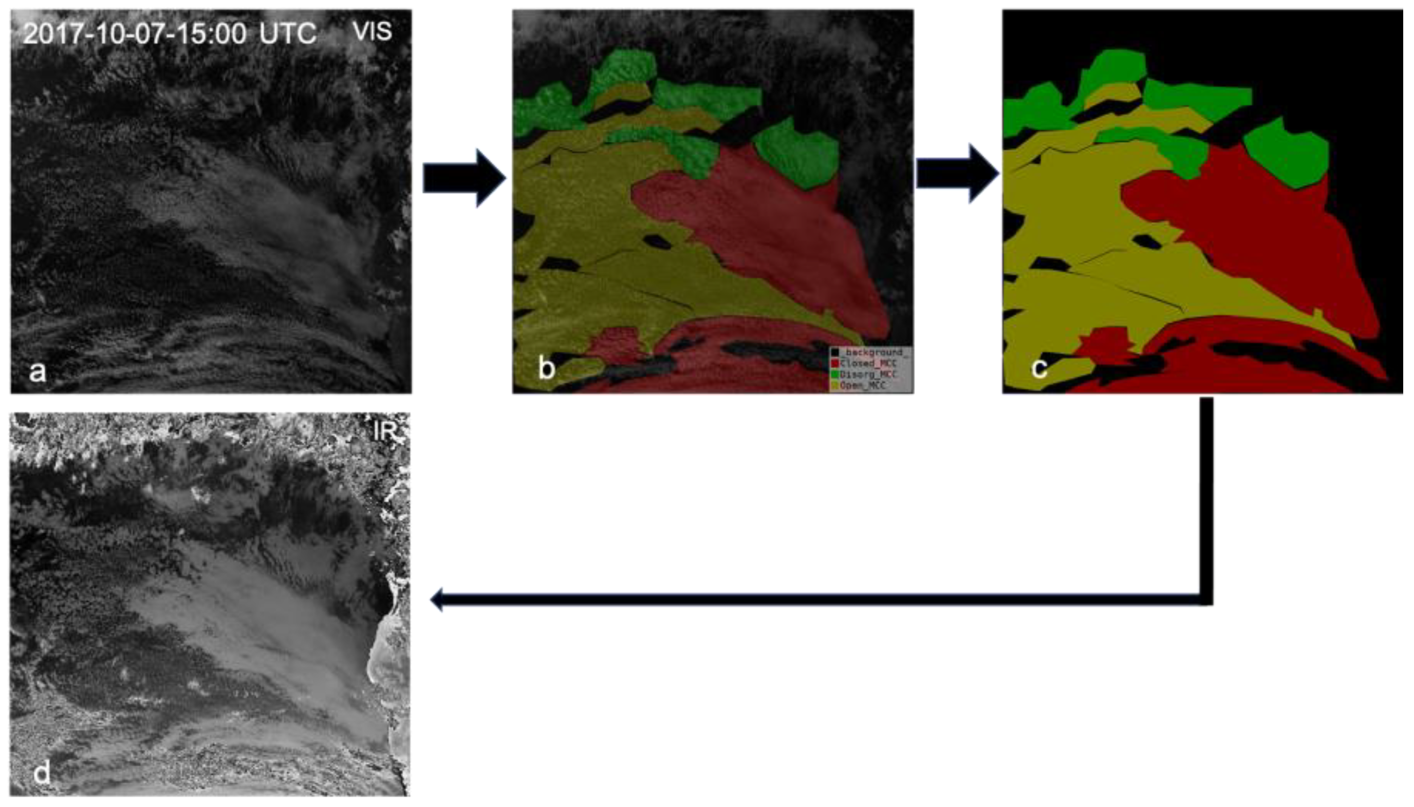
Figure 3.
An example of the labeling process used in training our cloud type MCC CNN network, with (a) a VIS image as an input to the labeling tool labelme [35], (b) the labeled polygons overlaid on the imagery, (c) the generated PNG discrete label map used as the ground-truth map in the training process, and (d) a scaled IR image that was used as an input to train the IR network, using the label map in (c) as the ground-truth map.

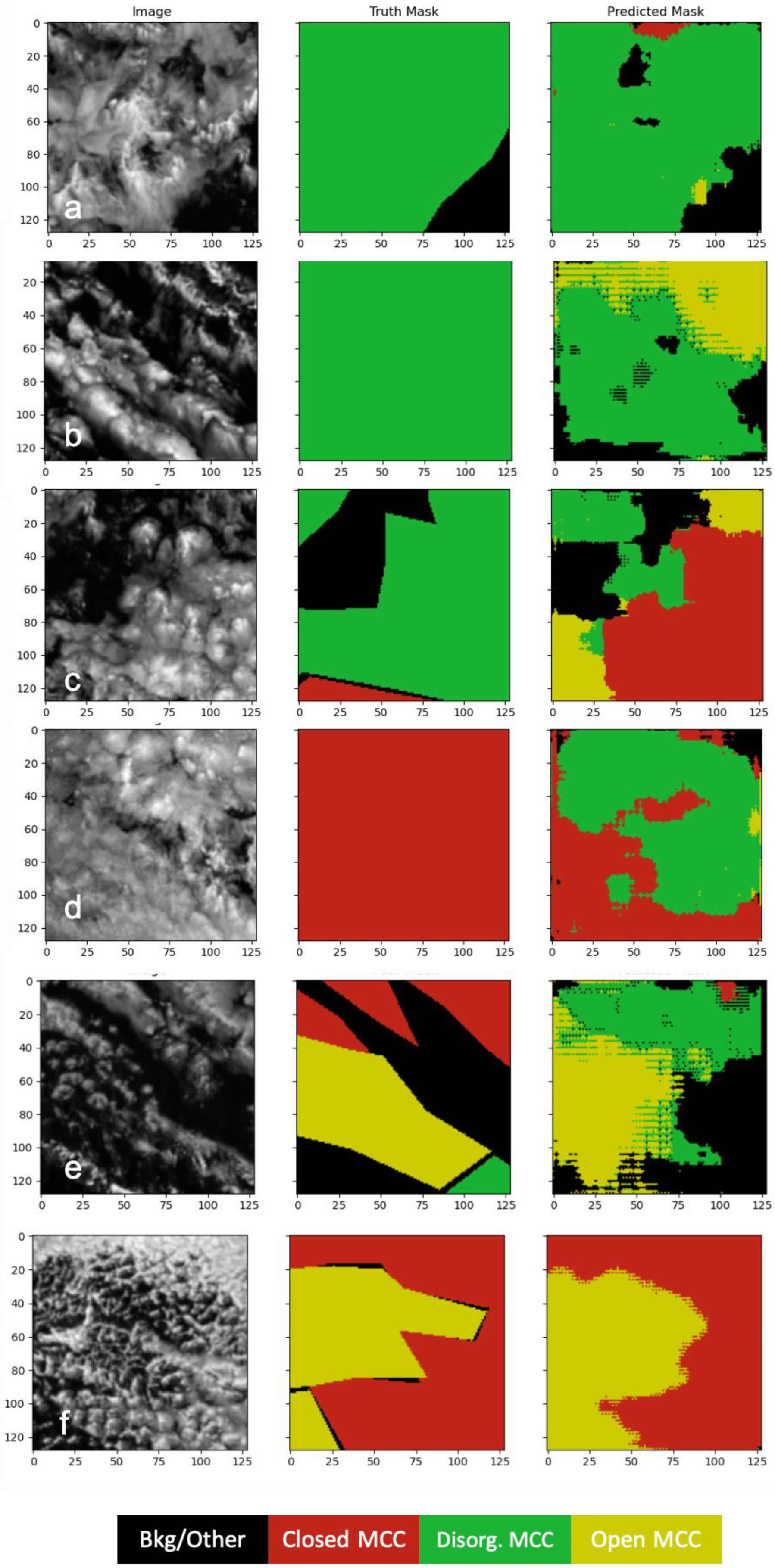
Figure 4.
Samples of 128 × 128 pixel patches used for prediction, where the left column shows the input VIS patch image, the center column shows the manually generated ground-truth map label used to calculate our test result accuracy, and the right column shows the class label prediction with (a) the manually labeled and correctly predicted disorg. class, (b) a manually labeled disorg. scene classified as partly disorg. and partly open MCC, (c) a manually labeled disorg. scene classified as closed MCC by the model, (d) a manually labeled closed MCC classified as partially closed MCC and partially disorg. (e) a mixed scene manually labeled as open and closed, classifying the closed label as disorg., and (f) manually labeled and correctly predicted closed and open MCC classes.

Figure 5.
(A) Confusion matrix showing random test patch prediction using the all-data VIS-model with the final selected architecture for the three-class model; (B) the same model as in (A), but predicting only patches with one (more than 97% of the pixels) main class; (C) single-patch model training prediction on random (multi-class) test patches. The highlighted CM in (B) represents the results that correspond to values obtained by the other available models trained using NN or CNN, as detailed in the text.

Figure 6.
(a) Visible channel input, (b) truth mask, and (c) prediction by the VIS-only model for a test scene on 5 September 2017, 10:00 UTC, and (d–f) similar but for the IR-only model prediction.
Figure 6.
(a) Visible channel input, (b) truth mask, and (c) prediction by the VIS-only model for a test scene on 5 September 2017, 10:00 UTC, and (d–f) similar but for the IR-only model prediction.

Figure 7.
Confusion matrix calculated for test-set images (a) for VIS-only prediction during daytime scenes, and (b) the same but for the IR-only model; (c) confusion matrix for VIS-only prediction during daytime and transition (08:00 and 16:00 UTC) scenes, and (d) the same as (c) but for IR model predictions.

Figure 8.
The left upper panels show the IR input, mask, and prediction triplet for 20 September 2017 at 20:00 UTC and the right upper panel shows its corresponding confusion matrix. The left lower panels show the IR input, mask, and prediction triplet for 25 September 2018 at 04:00 UTC and the right lower panel shows its corresponding confusion matrix.

Figure 9.
Probability distribution functions (PDFs) for all daylight hours (08:00–16:00 UTC) of four cloud properties retrieved from SEVIRI using the MODIS algorithm, with (a) showing COD (cloud optical depth), (b) Re (cloud effective radii), (c) LWP (liquid water path), and (d) Nd (cloud number concentration). Closed MCC is shown in solid blue lines and open MCC is shown in solid orange lines.

Figure 10.
Variations of closed (a) and open (b) MCC cloud type coverage during the BB season (August–October) over the SEA for 2016–2018.
Figure 10.
Variations of closed (a) and open (b) MCC cloud type coverage during the BB season (August–October) over the SEA for 2016–2018.

Figure 11.
Normalized probability density functions for (a) closed MCC and (b) open MCC derived by the current algorithm from SEVIRI (integrating 30 min. predictions) and (c) closed MCC and (d) open MCC derived by Yuan et al. [8]’s algorithm for the MODIS daytime overpass, aggregating data from the BB months (August–October) both over the SEA domain as defined in Figure 1.

Figure 12.
Domain area cloud coverage percentage for closed (blue) and open (orange) MCC cloud types, calculated using (a) all-day (30 min. interval) SEVIRI retrievals using the current work, (b) SEVIRI retrievals sampled at 13:30 local time to correspond with the MODIS overpass, and (c) Yuan et al. [8]’s retrievals from once-daily MODIS Aqua overpass.

Figure 13.
(a) Time of day (daytime only) fractional amount (where fraction represents the amount of pixels classified by a certain cloud type relative to the entire pixels over the research domain) for Closed, Open and Other cloud types, (b) same as a but for the entire diurnal cycle, where shaded area represents the 95% confidence interval margin based on the data standard deviation per each class, and (c) diurnal variability similar to b but parsed for each month (class color is similar to previous panels and months marked by different line types).

Figure 14.
Example of selected time-stamp predictions using the IR-only model on the GOES-ABI IR channel (10.3 mm) imagery as an input. IR images are shown on the left and prediction (with color code in the legend) on the right columns, respectively. Time is presented in both UTC and local time (LCT, which is UTC-5 in this region). White arrows represent areas of POC (pockets of open cells) in the corresponding images.

Figure 15.
Similar to Figure 13, but for the SEP region in 2018, as defined in text, presented at local time (UTC-5), showing (a) time of day (daytime only) fractional amount (where fraction represents the amount of pixels classified by a certain cloud type relative to the entire pixels over the research domain) for closed, open, and other cloud types; (b) the same as (a) but for the entire diurnal cycle, where the shaded area represents the 95% confidence interval margin based on the data standard deviation per each class, and (c) diurnal variability similar to (b) but parsed for each month (class color is similar to previous panels and months are marked by different line types).

Disclaimer/Publisher’s Note: The statements, opinions and data contained in all publications are solely those of the individual author(s) and contributor(s) and not of MDPI and/or the editor(s). MDPI and/or the editor(s) disclaim responsibility for any injury to people or property resulting from any ideas, methods, instructions or products referred to in the content. |
© 2023 by the authors. Licensee MDPI, Basel, Switzerland. This article is an open access article distributed under the terms and conditions of the Creative Commons Attribution (CC BY) license (https://creativecommons.org/licenses/by/4.0/).
Share and Cite
MDPI and ACS Style
Segal Rozenhaimer, M.; Nukrai, D.; Che, H.; Wood, R.; Zhang, Z. Cloud Mesoscale Cellular Classification and Diurnal Cycle Using a Convolutional Neural Network (CNN). Remote Sens. 2023, 15, 1607. https://doi.org/10.3390/rs15061607
AMA Style
Segal Rozenhaimer M, Nukrai D, Che H, Wood R, Zhang Z. Cloud Mesoscale Cellular Classification and Diurnal Cycle Using a Convolutional Neural Network (CNN). Remote Sensing. 2023; 15(6):1607. https://doi.org/10.3390/rs15061607
Chicago/Turabian StyleSegal Rozenhaimer, Michal, David Nukrai, Haochi Che, Robert Wood, and Zhibo Zhang. 2023. "Cloud Mesoscale Cellular Classification and Diurnal Cycle Using a Convolutional Neural Network (CNN)" Remote Sensing 15, no. 6: 1607. https://doi.org/10.3390/rs15061607
Note that from the first issue of 2016, this journal uses article numbers instead of page numbers. See further details here.