
Causes and Impacts of Decreasing Chlorophyll-a in Tibet Plateau Lakes during 1986–2021 Based on Landsat Image Inversion


1
State Key Laboratory of Tibetan Plateau Earth System, Environment and Resources (TPESER), Institute of Tibetan Plateau Research, Chinese Academy of Sciences, Beijing 100101, China
2
University of Chinese Academy of Sciences, Beijing 100049, China
3
Piesat Information Technology Co., Ltd., Beijing 100195, China
*
Author to whom correspondence should be addressed.
Remote Sens. 2023, 15(6), 1503; https://doi.org/10.3390/rs15061503
Submission received: 12 December 2022
/
Revised: 3 March 2023
/
Accepted: 6 March 2023
/
Published: 8 March 2023
Abstract
:Lake chlorophyll-a (Chl-a) is one of the important components of the lake ecosystem. Numerous studies have analyzed Chl-a in ocean and inland water ecosystems under pressures from climate change and anthropogenic activities. However, little research has been conducted on lake Chl-a variations in the Tibet Plateau (TP) because of its harsh environment and limited opportunities for in situ data monitoring. Here, we combined 95 in situ measured lake Chl-a concentration data points and the Landsat reflection spectrum to establish an inversion model of Chl-a concentration. For this, we retrieved the mean annual Chl-a concentration in the past 35 years (1986–2021) of 318 lakes with an area of > 10 km2 in the TP using the backpropagation (BP) neural network prediction method. Meteorological and hydrological data, measured water quality parameters, and glacier change in the lake basin, along with geographic information system (GIS) technology and spatial statistical analysis, were used to elucidate the driving factors of the Chl-a concentration changes in the TP lakes. The results showed that the mean annual Chl-a in the 318 lakes displayed an overall decrease during 1986–2021 (−0.03 μg/L/y), but 63%, 32%, and 5% of the total number exhibited no significant change, significant decrease, and significant increase, respectively. After a slight increase during 1986–1995 (0.05 μg/L/y), the mean annual lake Chl-a significantly decreased during 1996–2004 (−0.18 μg/L/y). Further, it decreased slightly during 2005–2021 (−0.02 μg/L/y). The mean annual lake Chl-a concentration was significantly negatively correlated with precipitation (R2 = 0.48, p < 0.01), air temperature (R2 = 0.31, p < 0.01), lake surface water temperature (LSWT) (R2 = 0.51, p < 0.01), lake area (R2 = 0.42, p < 0.01), and lake water volume change (R2 = 0.77, p < 0.01). The Chl-a concentration of non-glacial-meltwater-fed lakes were higher than those of glacial-meltwater-fed lakes, except during higher precipitation periods. Our results shed light on the impacts of climate change on Chl-a variation in the TP lakes and lay the foundation for understanding the changes in the TP lake ecosystem.
1. Introduction
Lakes serve as links in the interaction among the atmosphere, hydrosphere, and biosphere [1]. Lake ecosystems play a vital role in global climate change, biodiversity conservation, and human survival and development [2]. Moreover, lake water quality is an important index in studying the change in the lake ecosystem and its response to climate change [3,4,5]. Being affected by anthropogenic activities and climate change, global lakes have decreased in number, area, aquatic vegetation, and transparency; further, cyanobacterial blooms have been shown to be increasing in frequency and advancing temporally [6,7].
Lake chlorophyll-a (Chl-a), a critical pigment contained in various phytoplankton, serves as a crucial index in the evaluation of lake phytoplankton biomass, lake nutritional status, and lake ecosystem quality [8,9,10]. Chl-a concentration, together with the other parameters affecting optical features of lake water such as suspended particulate matter, colored dissolved organic matter (CDOM), and pure water, constitute the basis of water color remote sensing monitoring [11,12]. In this light, we can invert Chl-a concentration, suspended particulate concentration, water transparency, turbidity, dissolved organic matter, vertical attenuation coefficient of the incident and outgoing light in water, and a certain trophic state index through optical characteristics identified by spaceborne remote sensing [13,14].
The conventional remote sensing inversion models between water reflectance and lake Chl-a are mainly band ratio, band combination, multivariate statistical regression, stepwise regression, and exponentiation algorithm [15,16,17,18,19,20,21,22]. These statistical regression models are simple and with good interpretability, but they can barely solve the complex nonlinear relation of lake Chl-a and water reflectance, resulting in poor inversion accuracy. The classification-based algorithm system is complex and possibly possesses high precision, but the related parameters are difficult to obtain from the numerous studied objects. Machine learning, including the algorithms of backpropagation (BP) neural network, gaussian process regression (GPR), support vector regression (SVR), and random forest (RF) [23,24,25], constantly self-adjusts the relationships between independent and dependent variables and reduces the error and thus is an effective method to solve nonlinear regression problems. However, machine learning also needs to initially select possible relationships between independent and dependent variables for comparison, and sufficient measured data to train the inversion model to avoid “overfitting” or “overlearning” and the deteriorated model’s generalization ability [26,27].
In recent decades, several studies have analyzed the Chl-a in ocean and inland water ecosystems under pressure from climate change and anthropogenic activities [28,29,30,31,32]. However, little research has focused on lake Chl-a variations in the Tibet Plateau (TP) [33] because of its harsh environment and limited opportunities for in situ monitoring [34]. Most of the lakes on the TP are oligotrophic [35] and conduce low productivity under the cold climate [36]. The lake water optical properties in the TP are affected by not only Chl-a of phytoplankton, but also non-pigmented particles of other suspended matter and colored dissolved organic matter. Therefore, it is necessary to construct an adaptable inversion model based on in situ survey data to accurately invert lake Chl-a variations in the TP and detect their driving factors.
In this study, based on in situ survey data of Chl-a in the TP lakes, we combined the traditional band combination and BP neural network to establish an inversion model of lake Chl-a depending on Landsat water reflectance. The Chl-a values in the TP lakes from 1986–2021 were inverted for the analyses of their spatiotemporal changes. The hydrometeorological data and other water quality parameters of the lake basin in the TP were used to further analyze its affecting factors of lake Chl-a variations. Our research on lake Chl-a and its affecting factors can deepen the current understanding of the TP water quality, thus aiding in the performance and mechanism of the response of surface water environment to climate change in the area.
2. Study Area
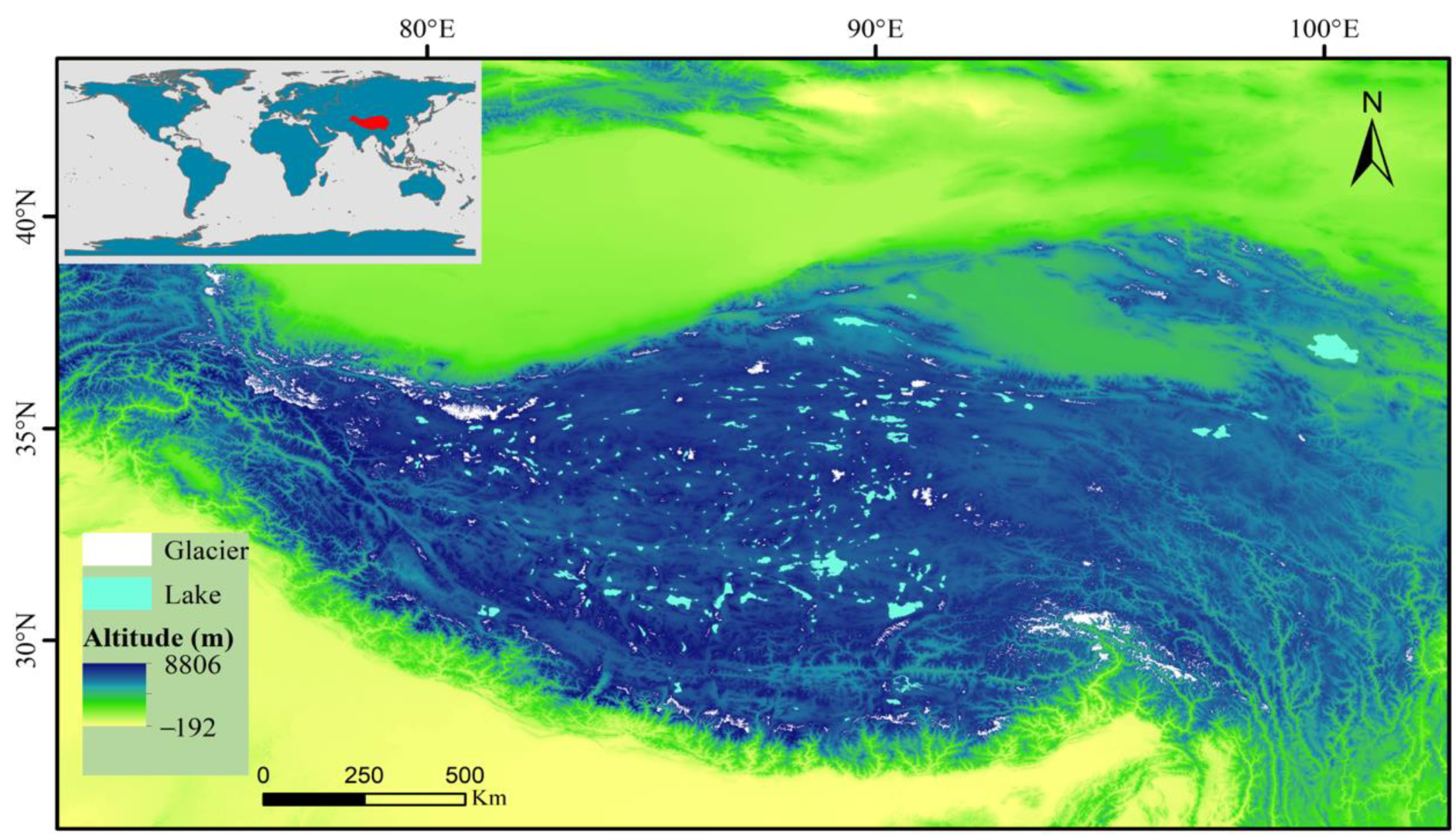
The TP (China territory) covers an area of ~2.57 million km2, ranging from 26°00′12″ N to 39°46′50″ N, 73°18′52″ E to 104°46′59″ E [37]. In 2018, there were more than 1400 lakes with an area of >1 km2, and a total area of ~50,000 km2 on the TP [38]. Most lakes are located in the alpine environment with >4000 m altitude where anthropogenic activities are scarce and weak. Most of the TP lakes are deeper than 30 m [39], with few aquatic vascular plants [40]. In recent decades, the variations in the TP lake physical features, such as lake area [41,42], water level [43,44], water volume [45,46,47,48,49,50], transparency [51], lake surface water temperature [52,53], and lake ice phenology [54,55,56], all respond significantly to the regional climate and environmental changes. These changes have inevitably exerted considerable effects on the lake ecosystem. In this study, we selected 318 TP lakes with an area of >10 km2 (occupying 95% of total TP lake area) as research objects (Figure 1). The second glacier inventory [57] revealed glacial meltwater replenishment in 180 of the 318 lake basins. The basin boundary data were obtained from HydroSHEDS (https://www.hydrosheds.org (accessed on 15 June 2022)).
3. Data and Methods
3.1. In Situ Measurement of Water Quality Parameters
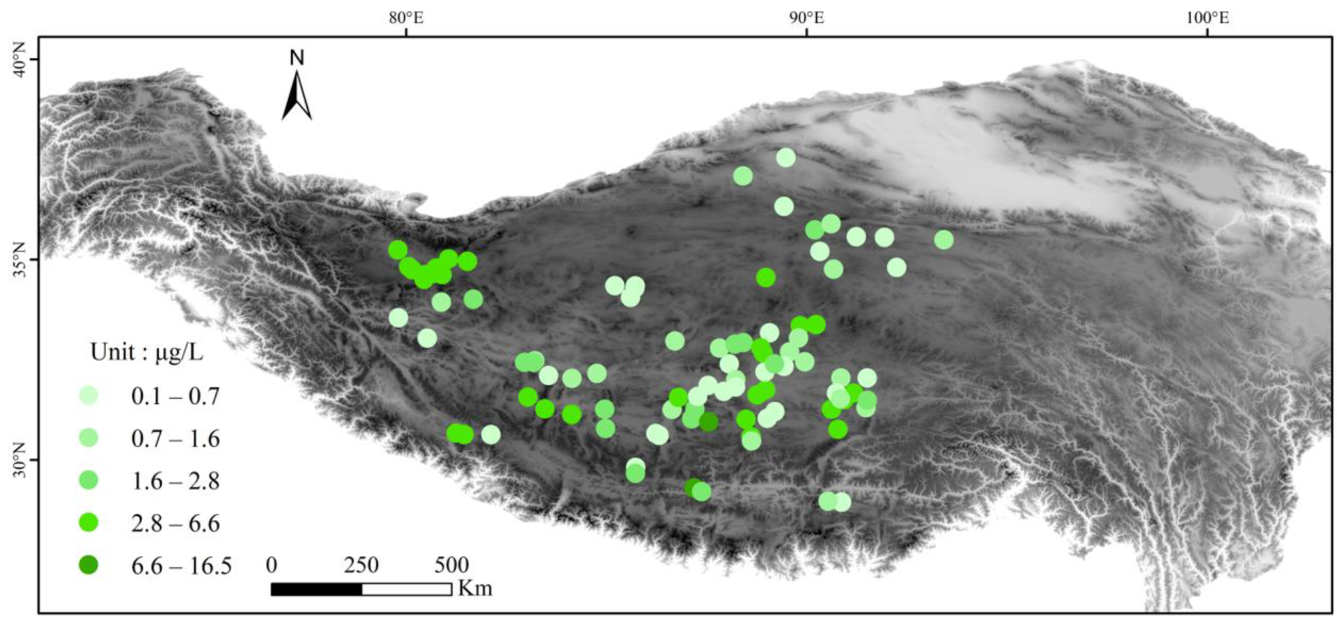
Water quality measurements were obtained from our long-term fieldwork investigation [35]. The water quality parameters, summarized in Supplementary Table S1, were measured by a widely used YSI EXO multi-parameter water quality instrument. The sensor or sampler was located at ~10–20 cm below the lake surface for both measurement and sample collection. The parameters included Chl-a concentration (95 samples), blue-green algae concentration (84 samples), turbidity (83 samples), pH (112 samples), dissolved oxygen (DO) (120 samples), fluorescent dissolved organic matter (fDOM) (54 samples), transparency (SD) (69 samples), and salinity (124 samples). Suspended matter concentration was calculated based on the water samples collected from lakes using filtration with Whatman glass fiber filters (pore size, 0.7 μm; diameter, 45 mm) followed by drying, calcination, and weighing (38 samples). To minimize the influence of the input runoff, we selected the central area of the lake or the open water area for measurement or sampling. The distribution of measured Chl-a data in 95 lakes is shown in Figure 2.
3.2. Climatic and Hydrological Factors
The China Meteorological Forcing Dataset (CMFD), with a temporal resolution of 3 h and spatial resolution of 0.1° [58], was used to estimate the mean annual temperature and precipitation in each lake basin. Lake surface water temperature (LSWT) was retrieved from the LSWT dataset collected across the Tibetan Plateau during 1978 to 2017 [59]. The lake area and water volume change data were acquired based on the research on the area and water volume change of lakes in the TP from 1976–2019 (relative to 1976) [60]. These data were accessed from http://www.tpdc.ac.cn (accessed on 15 July 2022) and had been widely used in previous studies conducted on the TP lake changes [61,62,63]. The glacier replenishment of the lake basin was analyzed based on the second glacier inventory dataset [57]. The altitude data were extracted from Digital Elevation Model (DEM) data in ArcGIS.
3.3. Remote Sensing Data and Processing Platform
The two datasets Landsat/LC05/C01/T1_SR and Landsat/LC08/C01/T1_SR (https://earthexplorer.usgs.gov/ (accessed on 15 January 2022)), containing land reflectance, were used for remote sensing inversions. These data were collected by Landsat-5 and Landsat-8 satellites for every 16 days crossing the investigated area. They contained five visible light and near-infrared (VNIR) bands and two short-wave infrared (SWIR) bands, and brightness temperature by two thermal infrared (TIR) bands. These data were processed to the L1TP level through precision and terrain correction. The two products of L5SR and L8SR are continuous and consistent, because the wavelengths of the bands of Landsat-5 and Landsat-8 do not change much. Several studies have successfully inverted water Chl-a by using Landsat-5 products and L5SR [64,65,66]. Furthermore, the LC08 SR product has been widely used in Chl-a inversion in water bodies of long time sequence with acceptable error [67,68,69,70]. To batch process the required Landsat surface reflectance data, we used the online remote sensing data processing platform Google Earth Engine (GEE, https://earthengine.google.com/ (accessed on 30 June 2022)).
3.4. Inversion Model Construction
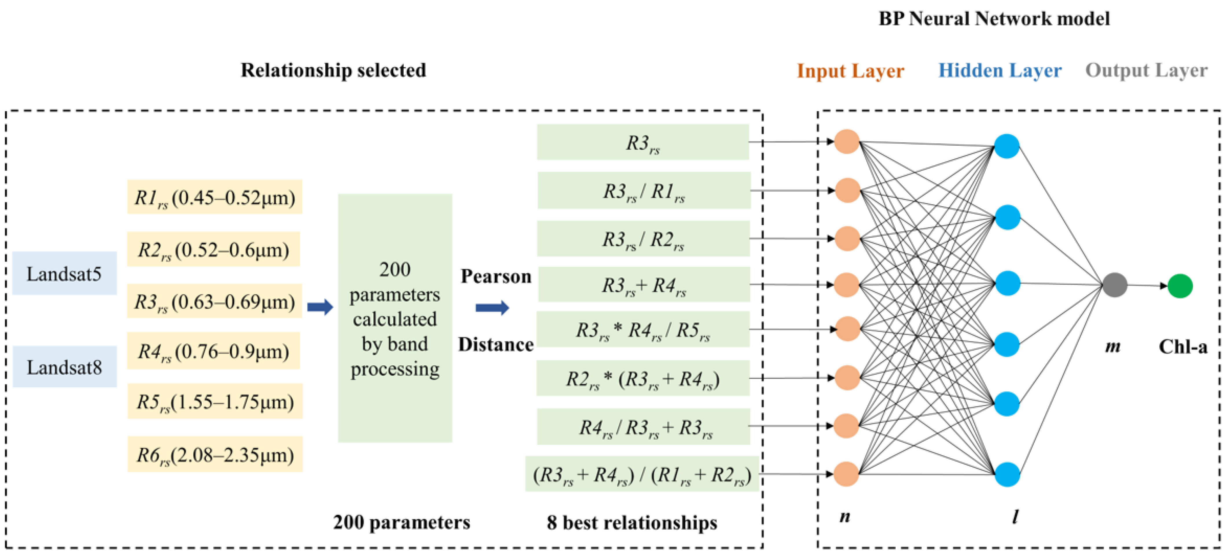
We selected six water reflectance bands of R1rs (0.45–0.52 μm), R2rs (0.53–0.59 μm), R3rs (0.64–0.67 μm), R4rs (0.85–0.88 μm), R5rs (1.57–1.65 μm), and R6rs (2.11–2.29 μm) in Landsat/LT08/C01/T1_SR images, which covered the ranges of our in situ measured data. We established 200 bands of combined parameters using the traditional band ratio, band combination, multiple linear regression, stepwise regression, and exponential algorithm. The satellite observation data with less than a 2-day time gap to the in situ measurement time were selected so that they were quasi-synchronous. Then, we applied the Pearson and Distance correlation coefficients to quantify the relationship coefficients (R) between established 200-band combined parameters and in situ measured Chl-a of 95 lakes in the TP. Eight functions, with a higher relationship coefficient between the band combined parameters and measured Chl-a, were selected as input sets for the machine learning algorithms of BP neural network, SVR, GPR, and RF. The calculation was performed in the MATLAB software. The coefficient of determination (R2), root mean square error (RMSE), mean absolute percentage error (MAPE), coefficient of variation (CV), slope, bias, and mean absolute error (MAE) [71] demonstrated that the inversion model of the BP neural network algorithm performed the best.
The selected BP neural network model, shown in the Supplementary Text S1, was comprised of three layers: input layer, hidden layer, and output layer. The input layer was composed of eight sub-nodes, representing eight higher relationship coefficient functions between the measured Chl-a and remote sensing reflectance band combined. The output layer was composed of only one neuron, reflecting the expected lake Chl-a concentration. As the measured samples of 95 lakes were insufficient, the excessive number of hidden layer nodes would inherently lead to a complex structure and poor generalization. Thus, we selected six hidden layer nodes. The overall framework of the inversion model is summarized in Figure 3.
The ten-fold cross-validation approach was used to test the model’s predictive ability and overfitting problem to evaluate the performance of each model efficiently [72]. Ten-fold cross-validation can randomly split all the samples into ten groups of nearly equal size. Each group was considered as the validation dataset to assess the model performance, while the rest of the nine groups were considered for the model fitting. This procedure was repeated ten times until each group was validated and assessed to make the corresponding predictions.
4. Results
4.1. Precisions of Inversion Model
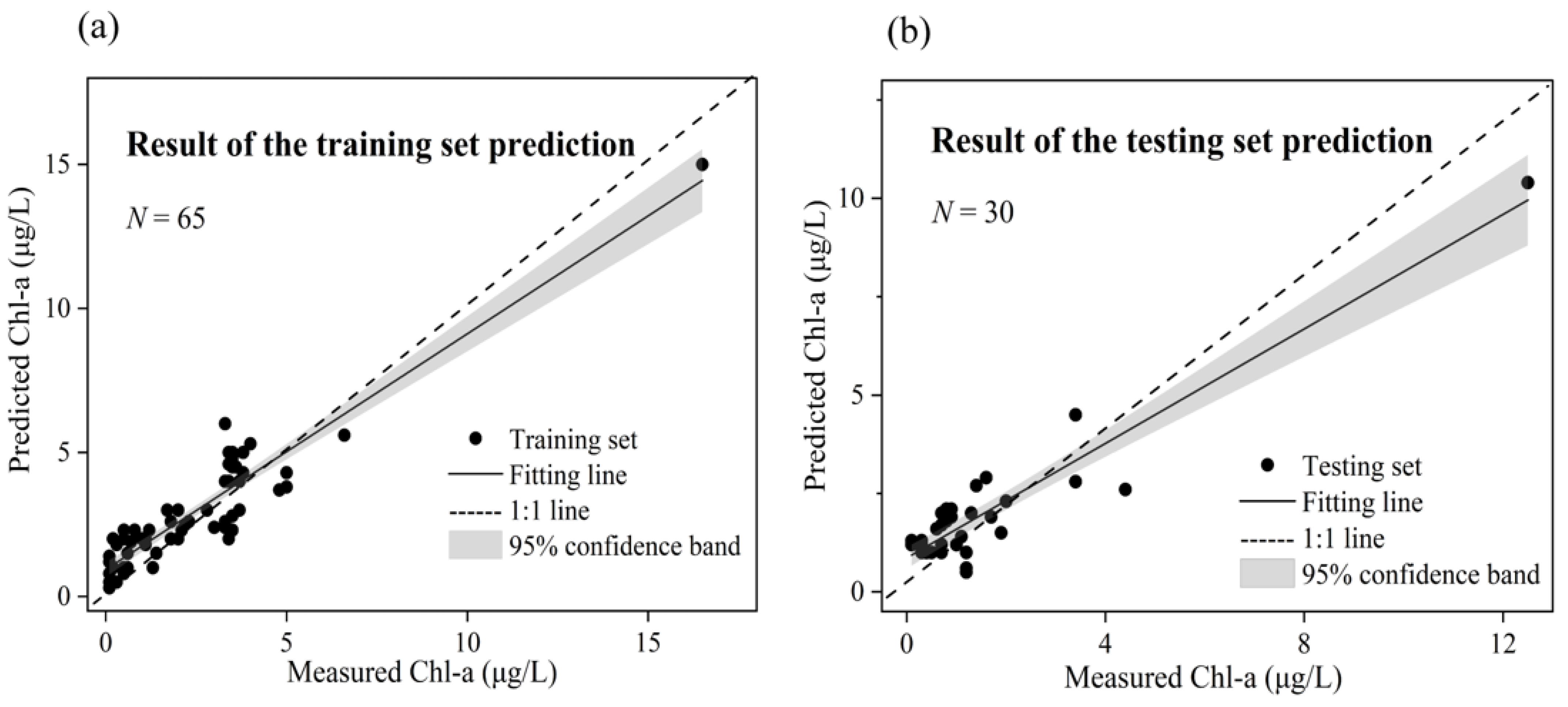
The water reflectances corresponding to the measured Chl-a of 95 lakes were input into the BP neural network model to retrieve the lake Chl-a inversion results, which were compared with the measured lake Chl-a data. We calculated the R2, RMSE, bias, MAE, CV, slope, and MAPE (Table 1) of the relationships between the estimated Chl-a values and in situ measured lake Chl-a to evaluate the model accuracy. In the ten-fold cross-validation test, the training set yielded the following metrics: R2 = 0.83, RMSE = 1.47, and bias = 1.33. The testing set yielded R2 = 0.85, RMSE = 1.21, and bias = 1.21 (Table 1). The error of inversion was acceptable, thus indicating the excellent performance of the inversion model (Figure 4).
4.2. Spatial Distribution of Lake Chl-a Concentration
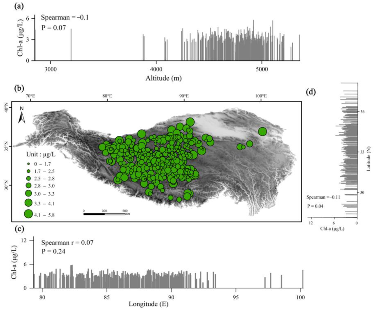
The mean annual water reflectances of Landsat from 1986–2021 in each lake area were processed on the GEE platform and input into the BP neural network model established by MATLAB to quantify lake Chl-a in the TP (Supplementary Table S2). We further examined the geographical distribution of lake Chl-a by calculating the multi-year average Chl-a concentration of the 318 lakes with an area > 10 km2 from 1986–2021 (Figure 5). No significant correlation (p > 0.01) between the lake Chl-a concentration and lake location (longitude and latitude) and altitude was discerned.
4.3. Spatial and Temporal Variations in Lake Chl-a Concentration
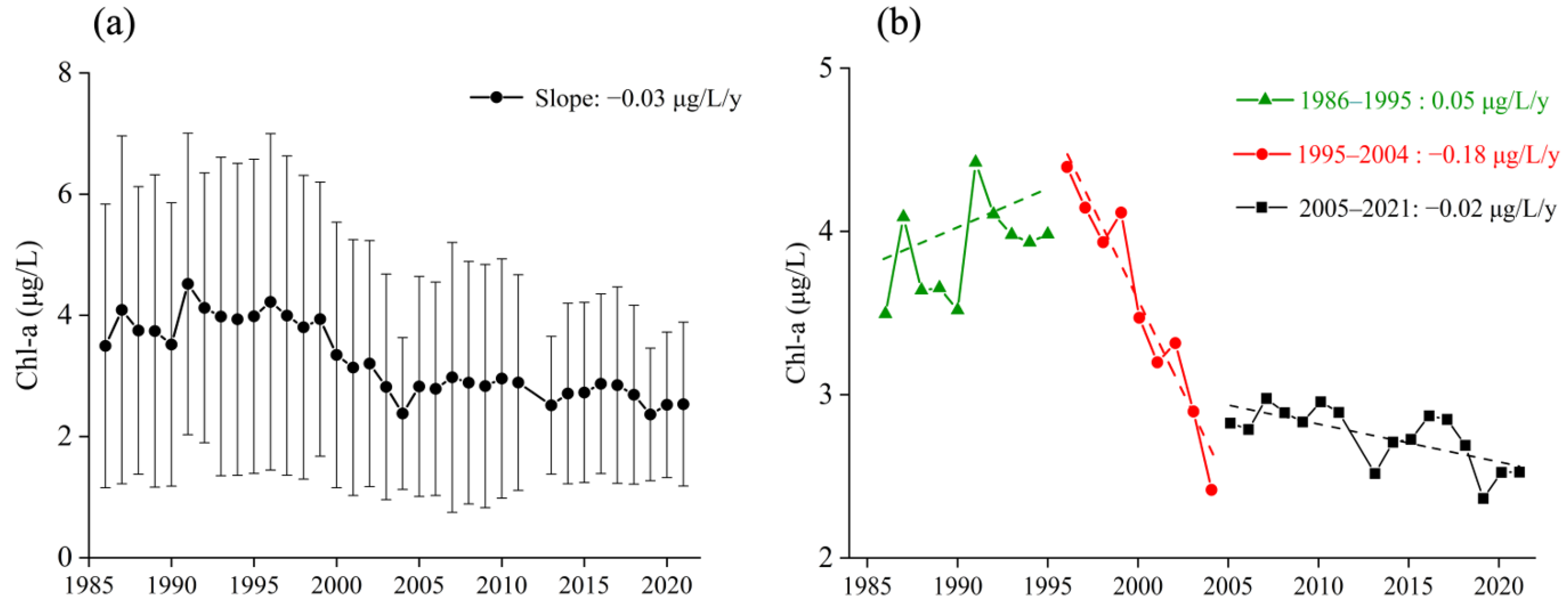
The mean annual Chl-a concentration in 318 lakes with an area > 10 km2 showed a general decreasing trend (−0.03 μg/L/y) from 1986–2021 (Figure 6a). We further analyzed the annual variation rate of these lakes’ mean annual Chl-a concentration and found that the three periods can be distinguished (Figure 6b). Lake Chl-a increased during 1986–1995 (0.05 μg/L/y), decreased significantly during 1996–2004 (−0.18 μg/L/y), and decreased slightly during 2005–2021 (−0.02 μg/L/y) (Figure 6b).
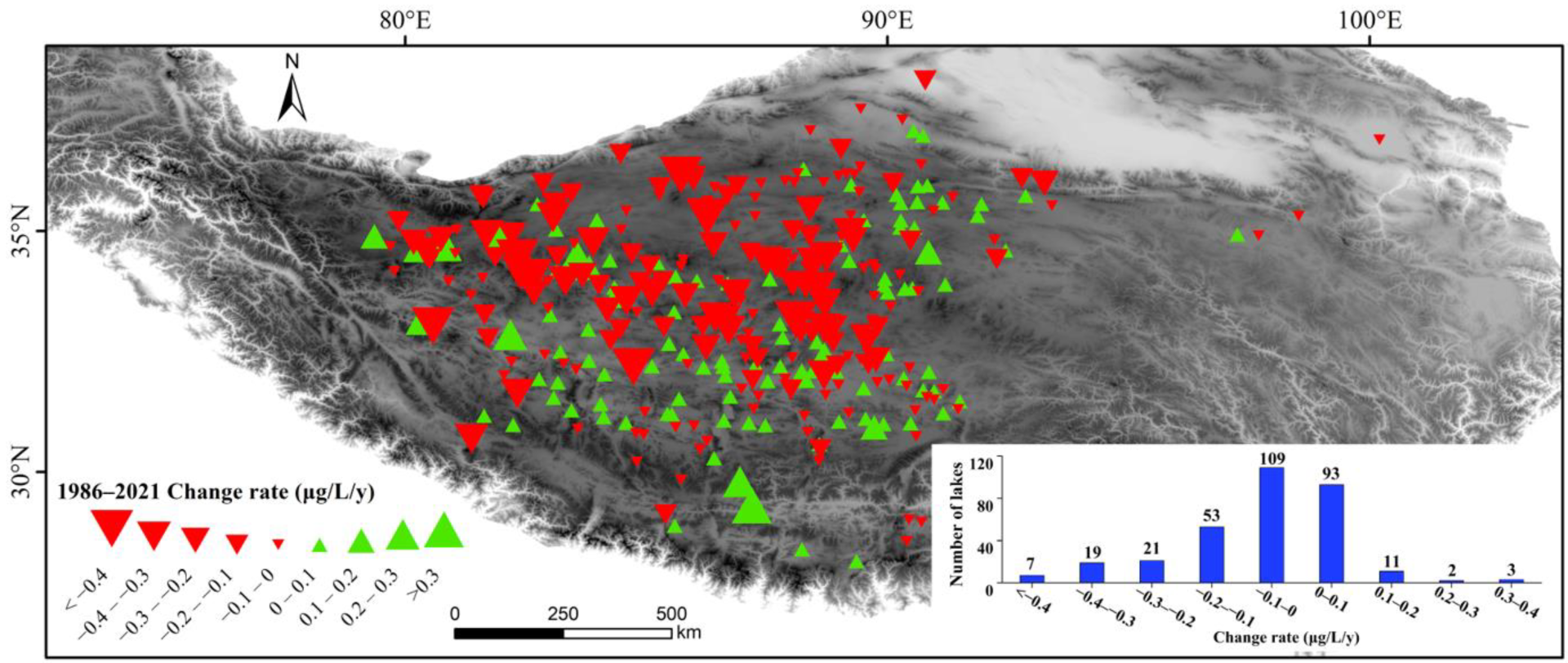
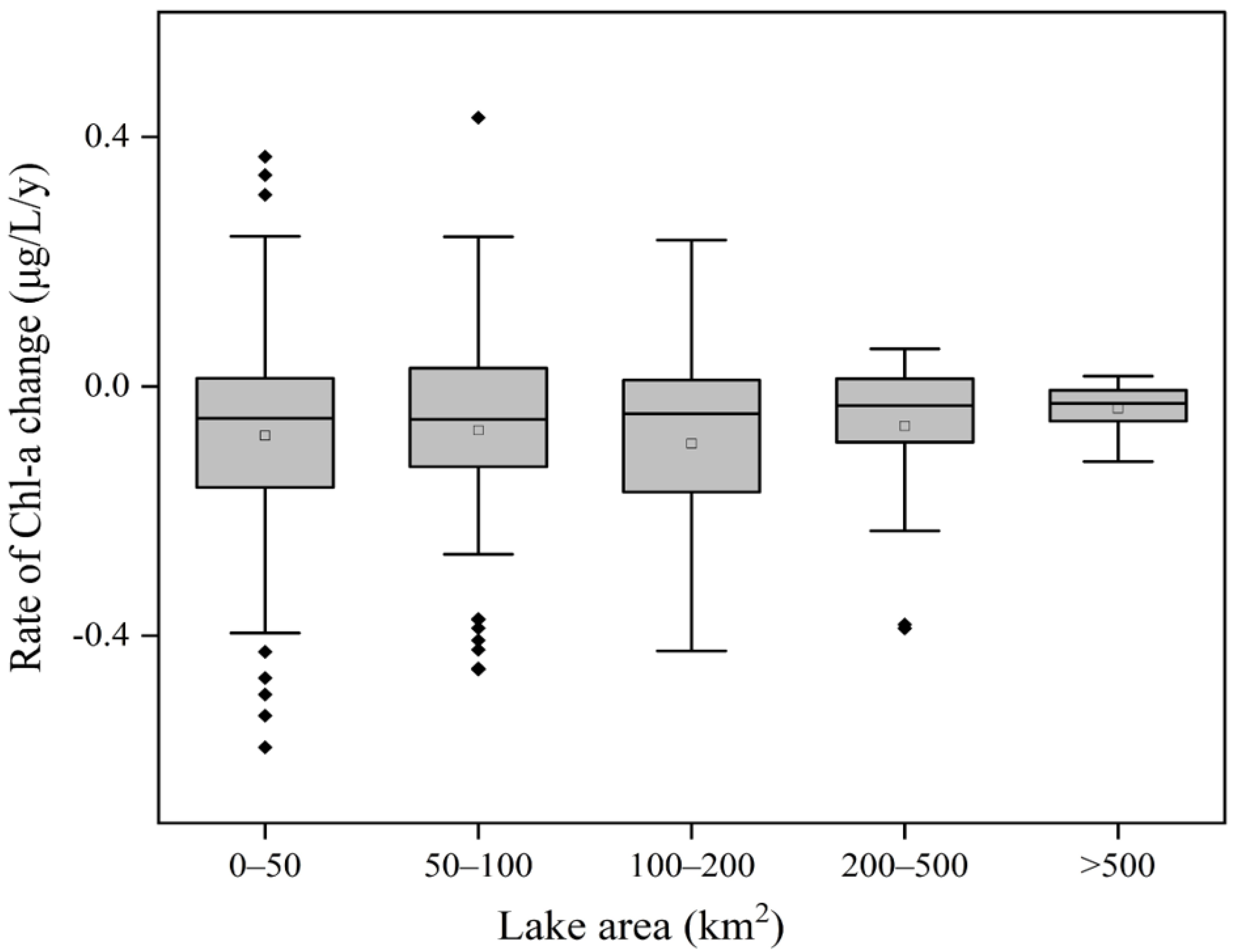
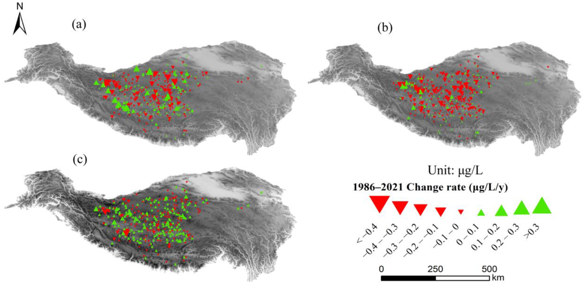
The rates of mean annual Chl-a concentration variation from 1986–2021 of the 318 lakes are shown in Figure 7. Although the mean annual variation rate of Chl-a concentration in most lakes generally exhibited no significant change, some lakes showed a decrease or an increase. Among them, 202 lakes (63%) showed no substantial change with the rate of –0.01 μg/L/y; 100 lakes (32%) showed significant decrease at the rate of –0.24 μg/L/y; and only 16 lakes (5%) exhibited an increase with a rate of 0.22 μg/L/y. During the study period, the Chl-a in several lakes of the northern TP significantly decreased (p < 0.01); in contrast, the Chl-a in most lakes of the southern TP increased significantly (p < 0.05), as shown in Figure 7. The annual variation in Chl-a in large lakes (area > 200 km2) was weak and tended to be stable (Figure 8).
From 1986–1995, although the overall variation in lake Chl-a exhibited an increasing trend, the number of lakes with increased Chl-a was lower than that of lakes with decreased Chl-a; however, lakes with increased Chl-a exhibited higher Chl-a increase rates, and only a few lakes in the northern and northwestern TP exhibited higher Chl-a decrease rates (Figure 9a). From 1996–2004, the Chl-a generally decreased, with a higher decline rate in the northern TP; only a few lakes in the northwestern TP exhibited Chl-a increase (Figure 9b). From 2005–2021, while there was a significant increase in the number of lakes with increasing Chl-a concentration, their increasing amplitude was still lower than the amplitude of the decline in lakes with decreasing Chl-a concentration in the same period (Figure 9c).
5. Discussion
5.1. Influence of Climate Change on Lake Chl-a
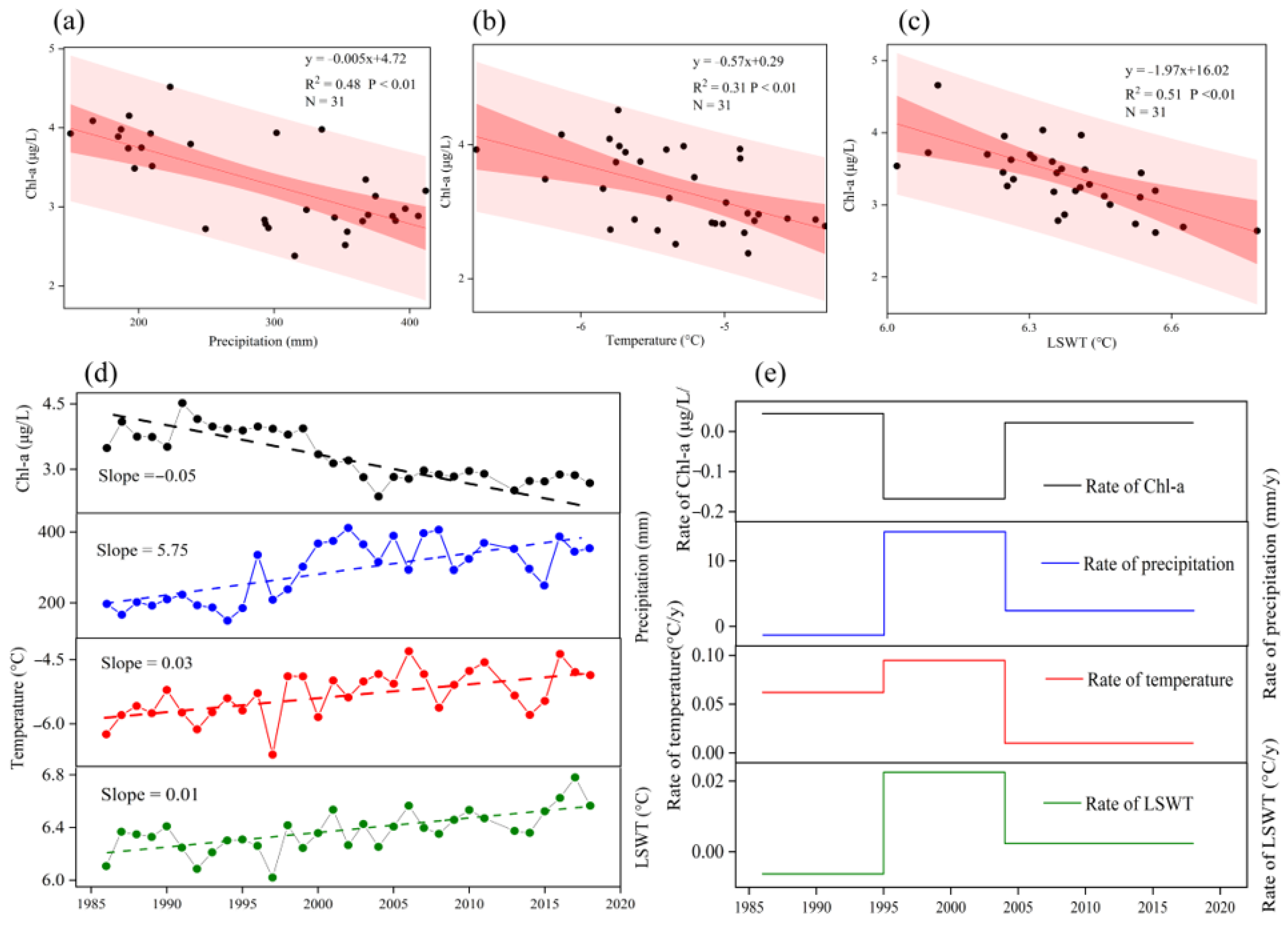
Precipitation and temperature have apparent effects on lake ecosystem [73,74]. LSWT is a sensitive indicator to climate change and its changing amplitude is even surpassing that of air temperature change under global warming [75,76]. The mean annual Chl-a concentration was significantly negatively correlated with precipitation (R2 = 0.48, p < 0.01), temperature (R2 = 0.31, p < 0.01), and LSWT (R2 = 0.51, p < 0.01) (Figure 10a–c) in the TP lakes. Precipitation, temperature, and LSWT all increased from 1986–2018, while lake Chl-a generally decreased (Figure 10d), but they exhibited inconsistent variation trends in different periods (Figure 10e). From 1986–1995, precipitation decreased slightly, whereas temperature, LSWT, and Chl-a exhibited a weak increase. From 1996–2004, precipitation, temperature, and LSWT showed a rapid increase, whereas lake Chl-a decreased. From 2005–2017, precipitation showed an insignificant increase, whereas temperature, LSWT, and lake Chl-a slowly decreased or remained almost unchanged (Figure 10e).
Correlation analysis showed that temperature and precipitation significantly affected lake Chl-a concentration. Although precipitation and its derived runoff might bring dissolved and suspended components and terrestrial organic matter into the lake, thus potentially promoting the growth of phytoplankton [77], increased precipitation in lake basins may exert the opposite effect on lake ecosystems in the TP. The clean atmosphere of the TP is conducive to the very low mineral nutrients contained in precipitation, and the scarce vegetation cover in the TP implies that the runoff formed by precipitation carries less terrestrial organic matter into the lake. Even if the nutrients from precipitation can promote the growth of lake phytoplankton, the increase in lake water volume caused by precipitation exceeds the increase in nutrients, thereby resulting in the decrease in nutrients and lake Chl-a density [78,79,80]. A similar correlation between precipitation and Chl-a has been previously reported in other regions [81,82].
Climate warming tends to increase or decrease Chl-a concentration in phytoplankton-rich or -deficient lakes, respectively [83]. An investigation of TP lakes found fish only in lakes with salinity less than 7 g/L in the total investigated lakes [84]. They concluded that the ratio of Chl and total phosphorus was positively related to temperature in lakes with predators, and negatively in lakes without predators. For most saline or salty lakes in TP with no predators (such as fishes or gammarid), there are only two trophic levels: phytoplankton and zooplankton. Rising temperature would benefit zooplankton development, which then restrains phytoplankton growth [84]. Therefore, only 1/3 of the 318 studied lakes showed decreased Chl-a concentration during 1986–2021, but these lakes predominated the generally decreasing tendency because the remaining 2/3 of the lakes showed no changes. In fact, greater understanding of the physiological processes of lake phytoplankton is still needed for elucidating the phytoplankton biomass variation under future climate warming [85].
5.2. Influence of Lake Area, Volume Change, and Glacier Replenishment Type on Lake Chl-a
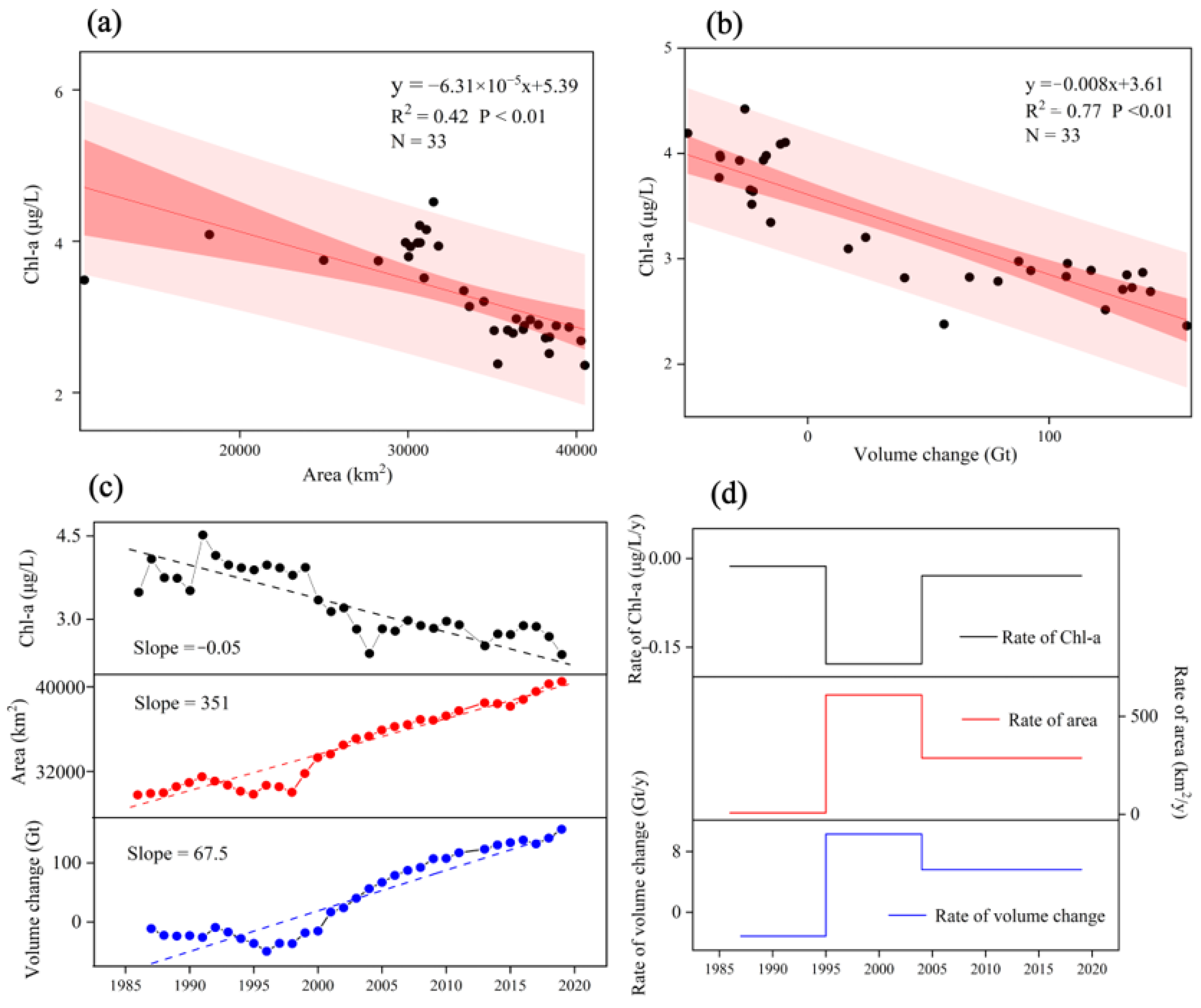
During 1986–2019, significant negative correlations between lake Chl-a and lake area and volume change (R2 = 0.42, p < 0.01; R2 = 0.77, p < 0.01) were found (Figure 11a,b). As lake area and volume increased, lake Chl-a decreased (Figure 11c), a finding which was consistent with the unvalidated inversion results that Chl-a concentration in large lakes was lower than that in small lakes [33]. However, their variability rates were not always consistent among different periods (Figure 11d). From 1986–1995, although lake area increased slightly, lake water volume and lake Chl-a exhibited a weaker decrease. From 1996–2004, both lake area and water volume increased, whereas lake Chl-a decreased rapidly. From 2005–2019, with the slowing rate of increase in lake area and water volume, lake Chl-a decreased gradually or remained nearly unchanged.
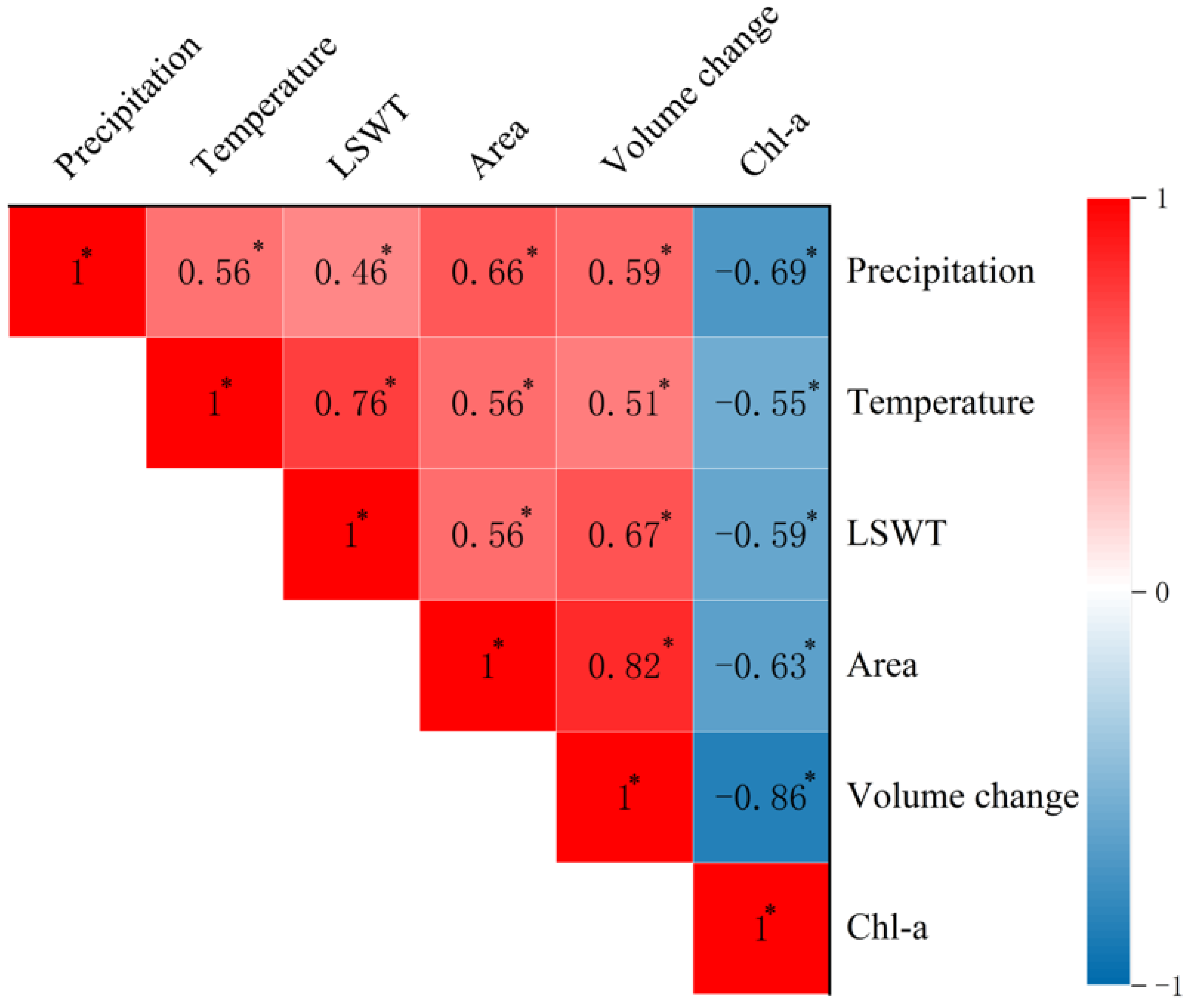
We further used the correlation coefficient method to analyze the degree of impact of meteorological and hydrological factors (temperature, precipitation, LSWT, area, and volume change) on lake Chl-a. The correlation coefficient between lake volume change and lake Chl-a showed the highest value, indicating that the lake volume change was the main cause of lake Chl-a variations (Figure 12). The lake water volume in the central and northern TP increased, whereas that in southern TP decreased, which also supports our results: the Chl-a in several lakes of the northern TP decreased significantly, whereas that in most lakes of the southern TP increased significantly.
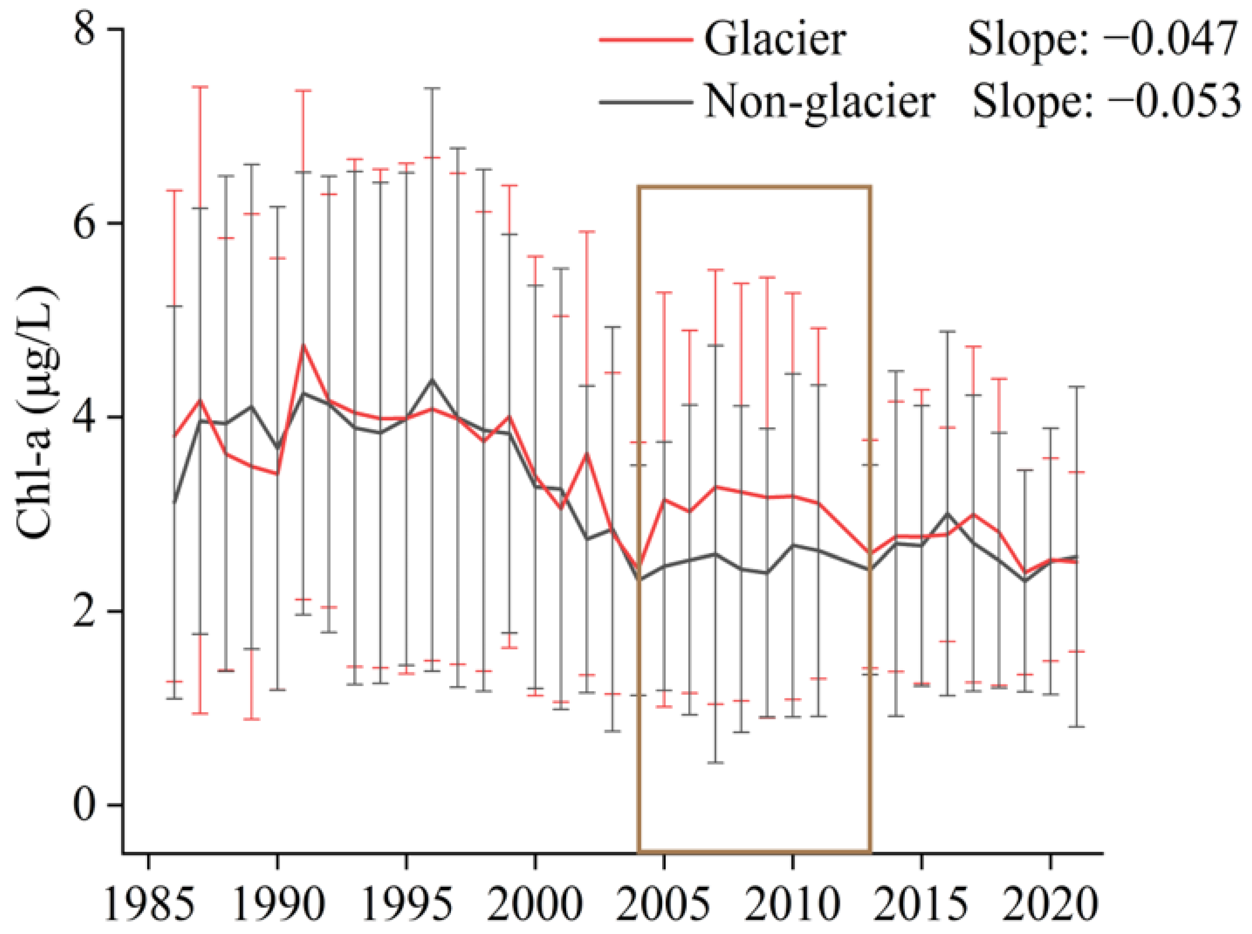
The widespread glaciers on the TP have been considered as an essential factor in the accelerated change of lakes in recent decades [42,45]. The decrease in water temperature and the increase in light attenuation in meltwater-related lakes can regulate the growth of phytoplankton, thus affecting lake Chl-a concentration [86,87]. Of the 318 lakes, we compared the mean annual Chl-a in 180 lakes fed by glacial meltwater with that in the lakes without glacial meltwater. The slope of Chl-a in glacial-meltwater-fed lakes was higher than that in non-glacial-meltwater-fed lakes (p = 0.005) (Figure 13), and this trend was mainly derived from the significant difference noted during 2004–2013 (p = 0.0002). There was no significant difference between these two in other periods. This was probably due to the stronger increase in precipitation during this period, which was conducive for decreased Chl-a in lakes that were replenished only by precipitation.
5.3. Influence of Lake Water Quality Parameters on Lake Chl-a
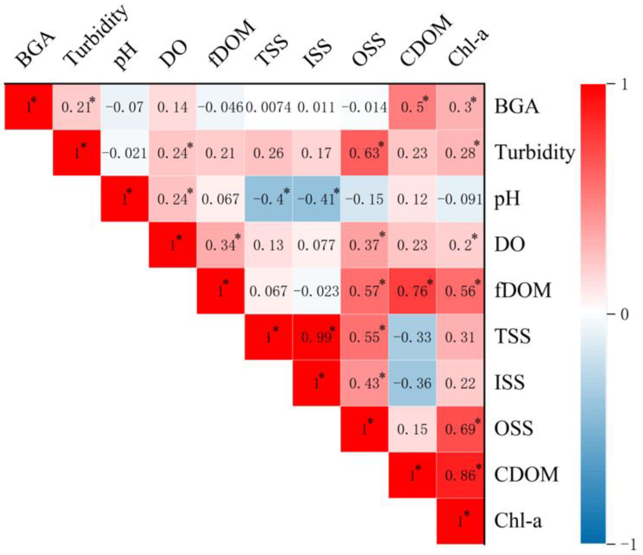
Lake Chl-a is the most direct response of the lake ecosystem quality, which is unavoidably affected by other factors [8,9]. We further analyzed the relationships between lake Chl-a and other water quality parameters based on the measured data of total suspended solids (TSS), inorganic suspended solids (ISS), organic suspended solids (OSS), turbidity, colored dissolved organic matter (CDOM), fluorescent-colored dissolved organic matter (fDOM), dissolved oxygen (DO), blue-green algae (BGA), and pH (Figure 14).
The backward scattering coefficient of suspended solids exerted a direct nonlinear effect on water reflectivity [86], while the Chl-a concentration was positively correlated with the concentration of suspended solids, including total, organic, and inorganic suspended solids. The relationship of Chl-a with OSS (R = 0.69, p < 0.01) was stronger than that with ISS (R = 0.22, p > 0.05). Thus, it is reasonable to infer that the content of inorganic suspended solids did not have a significant effect on nutrients utilized by phytoplankton [88]. Moreover, lake Chl-a was positively correlated with turbidity (R = 0.28, p < 0.05), indicating that highly turbid lakes exhibited high Chl-a concentration, and vice versa. Turbidity is the result of the scattering and absorption of light from particles in water. Scattering is mainly caused by suspended particulate matter, while absorption is partially driven by lake Chl-a and colored dissolved or particulate matter [89]. Therefore, increased turbidity is related to increased suspended matter or lake Chl-a and colored dissolved matter.
CDOM is one of the measurable optical components in relation to water color change of dissolved organic matters [90,91,92]. CDOM can also reflect the indirect correlation between salinity and water color in estuaries or coastal regions [93,94]. fDOM is an ideal substitution for CDOM and has been widely used to study water environments because it can be simply and efficiently measured [95,96,97,98]. fDOM is significantly correlated with CDOM [99,100] and can be used to calculate CDOM concentration using different algorithms and wavelength absorption coefficients [101]. In this study, we utilized an absorption coefficient at 375 nm because absorption coefficients in shorter wavelengths tend to better describe CDOM in clean water environments compared with longer wavelengths [102,103]. Although the concentrations of CDOM and fDOM in the studied lakes were low, fDOM, CDOM, and Chl-a were significantly positively correlated with each other (R = 0.56, p < 0.01; R = 0.86, p < 0.01). These findings indicate that phytoplankton in the oligotrophic lakes are still strongly associated with dissolved organic matter.
DO has a relationship with phytoplankton metabolism [104]. In this study, DO was found to be weakly but positively correlated with Chl-a (R = 0.20, p < 0.05). This is probably because increased photosynthesis of phytoplankton may consume CO2 in the water and produce DO. Cyanobacteria, as a component of phytoplankton, was significantly positively correlated with Chl-a (R = 0.30, p < 0.05), whereas Chl-a had a weak relationship with pH. The correlation coefficient analyses, except CDOM and fDOM, which are closely linked with Chl-a, showed that OSS is the key factor impacting Chl-a variations.
5.4. Limitations and Suggestions for Future Work
This study focused on lake Chl-a concentration inversion based on the water reflectance of Landsat images and lake Chl-a changes in the TP lakes. Although we have shown the relationships between lake Chl-a and the environmental factors of lakes in the TP, more detailed investigations are still needed to assess the causes of lake Chl-a changes. First, the timing of the in situ measuring of lake Chl-a did not correspond well with the satellite crossing dates due to the low temporal resolution of Landsat images. This is possible to conduce to the relatively large inversion error based on the remote sensing reflectance. Second, the knowledge was limited on the nutrients necessary for lake phytoplankton growth and on the water color influenced by phytoplankton composition. This led to a very weak explanation of relationships among Chl-a and other water quality parameters. Third, the negative relationship between Chl-a and temperature was only based on the statistical analyses. The cumulative effect of climate warming on phytoplankton biomass remains unclear for most global lakes, especially in the TP. Therefore, it is necessary to use remote sensing data with higher temporal and spectral resolution for inverse Chl-a concentration and discern a greater detail of its relationship with water quality. The nutrient components necessary for different phytoplankton growth and their relations with salinity require further investigation. Seasonal Chl-a monitoring in the lakes needs to be carried out to detect the relations between temperature changes and Chl-a variations.
6. Conclusions
This study analyzed the spatiotemporal variation patterns and influencing factors of Chl-a in the TP lakes. The following key conclusions were drawn:
- A comparison between the measured lake Chl-a concentration and remote sensing reflectance inversion data demonstrated that the inversion of Chl-a of the TP lakes by the BP neural network prediction model was remarkable.
- Lake Chl-a concentration increased during 1986–1995, while a significant decline period was identified during 1996–2004, with finally a slight increase during 2005–2021.
- The mean annual Chl-a concentration in the TP lakes was significantly negatively correlated with precipitation, temperature, LSWT, lake area, and lake water volume change in the study region. With an increase in precipitation, temperature, and lake area, Chl-a concentration exhibited a downward trend. Chl-a concentration of non-glacial -meltwater-fed lakes was higher than that of glacial-meltwater-fed lakes, except during periods of higher precipitation.
Supplementary Materials
The following supporting information can be downloaded at: https://www.mdpi.com/article/10.3390/rs15061503/s1, Table S1: In situ measured lake water quality parameters; Table S2: Inversion of Chl-a concentration; Text S1: BP neutral net model.
Author Contributions
Conceptualization, L.Z. and S.P.; methodology, S.P.; software, S.P.; validation, C.L., J.J. and S.P.; formal analysis, S.P.; investigation, L.Z., C.L. and J.J.; resources, L.Z., C.L. and J.J.; data curation, L.Z., C.L., and J.J.; writing—original draft preparation, S.P.; writing—review and editing, L.Z., C.L. and J.J.; visualization, S.P.; supervision, L.Z.; project administration, L.Z.; funding acquisition, L.Z. All authors have read and agreed to the published version of the manuscript.
Funding
This research was funded by the National Nature Science Foundation of China (41831177), Second Tibetan Plateau Scientific Expedition and Research (STEP) (2019QZKK0202), CAS Strategic Priority Research Program (XDA20020100 and XDA19020303), and CAS Alliance of Field Observation Stations (KFJ-SW-YW038).
Data Availability Statement
The data of experimental images used to support the findings of this research are available from the corresponding author upon reasonable request.
Conflicts of Interest
The authors declare no conflict of interest.
References
- Williamson, C.E.; Saros, J.E.; Vincent, W.F.; Smol, J.P. Lakes and reservoirs as sentinels, integrators, and regulators of climate change. Limnol. Oceanogr. 2009, 54, 2273–2282. [Google Scholar] [CrossRef]
- Tranvik, L.J.; Downing, J.A.; Cotner, J.B.; Loiselle, S.A.; Striegl, R.G.; Ballatore, T.J.; Dillon, P.; Finlay, K.; Fortino, K.; Knoll, L.B. Lakes and reservoirs as regulators of carbon cycling and climate. Limnol. Oceanogr. 2009, 54, 2298–2314. [Google Scholar] [CrossRef] [Green Version]
- Crossman, J.; Futter, M.N.; Oni, S.K.; Whitehead, P.G.; Jin, L.; Butterfield, D.; Baulch, H.M.; Dillon, P.J. Impacts of climate change on hydrology and water quality: Future proofing management strategies in the Lake Simcoe watershed, Canada. J. Great Lakes Res. 2013, 39, 19–32. [Google Scholar] [CrossRef]
- Zhang, X.Q.; Sun, R.; Zhu, L.P. Lake Water in the Yamzhog Yumco Basin in South Tibetan Region: Quality and Evaluation. J. Glaciol. Geocryol. 2012, 34, 950–958. [Google Scholar]
- Zhang, Y.Y.; Hua, R.X.; Xia, R. Impact Analysis of Climate Change on Water Quantity and Quality in the Huaihe River Basin. J. Nat. Resour. 2017, 32, 114–126. [Google Scholar]
- Verburg, P.; Hecky, R.E.; Kling, H. Ecological consequences of a century of warming in Lake Tanganyika. Science 2003, 301, 505–507. [Google Scholar] [CrossRef] [Green Version]
- Zhang, F.F.; Li, J.S.; Shen, Q.; Zhang, B.; Wu, C.Q.; Wu, Y.F.; Wang, G.L.; Wang, S.L.; Lu, Z.Y. Algorithms and Schemes for Chlorophyll a Estimation by Remote Sensing and Optical Classification for Turbid Lake Taihu, China. IEEE J. Sel. Top. Appl. Earth Obs. Remote Sens. 2015, 8, 350–364. [Google Scholar] [CrossRef]
- Gons, H.J.; Auer, M.T.; Effler, S.W. MERIS satellite chlorophyll mapping of oligotrophic and eutrophic waters in the Laurentian Great Lakes. Remote Sens. Environ. 2008, 112, 4098–4106. [Google Scholar] [CrossRef]
- Guildford, S.J.; Hecky, R.E. Total nitrogen, total phosphorus, and nutrient limitation in lakes and oceans: Is there a common relationship? Limnol. Oceanogr. 2000, 45, 1213–1223. [Google Scholar] [CrossRef] [Green Version]
- Lyche-Solheim, A.; Feld, C.K.; Birk, S.; Phillips, G.; Carvalho, L.; Morabito, G.; Mischke, U.; Willby, N.; Søndergaard, M.; Hellsten, S. Ecological status assessment of European lakes: A comparison of metrics for phytoplankton, macrophytes, benthic invertebrates and fish. Hydrobiologia 2013, 704, 57–74. [Google Scholar] [CrossRef] [Green Version]
- Mancino, G.; Nole, A.; Urbano, V.; Amato, M.; Ferrara, A. Assessing water quality by remote sensing in small lakes: The case study of Monticchio lakes in southern Italy. iFor.-Biogeosci. For. 2009, 2, 154–161. [Google Scholar] [CrossRef] [Green Version]
- Wu, G.F.; Cui, L.J.; Duan, H.T.; Fei, T.; Liu, Y.L. Absorption and backscattering coefficients and their relations to water constituents of Poyang Lake, China. Appl. Opt. 2011, 50, 6358–6368. [Google Scholar] [CrossRef]
- Binding, C.E.; Greenberg, T.A.; Bukata, R.P. The MERIS Maximum Chlorophyll Index; its merits and limitations for inland water algal bloom monitoring. J. Great Lakes Res. 2013, 39, 100–107. [Google Scholar] [CrossRef]
- Li, S.J.; Wang, X.J. The Spectral Features Analysis and Quantitative Remote Sensing Advances of Inland Water Quality Parameters. Geogr. Territ. Res. 2002, 18, 26–30. [Google Scholar]
- Gons, H.J. Optical teledetection of chlorophyll a in turbid inland waters. Environ. Sci. Technol. 1999, 33, 1127–1132. [Google Scholar] [CrossRef]
- Gurlin, D.; Gitelson, A.A.; Moses, W.J. Remote estimation of chl-a concentration in turbid productive waters—Return to a simple two-band NIR-red model? Remote Sens. Environ. 2011, 115, 3479–3490. [Google Scholar] [CrossRef]
- Huang, Y.H.; Jiang, D.; Zhuang, D.F.; Fu, J.Y. Research on remote sensing estimation of chlorophyll concentration in water body of Tangxun Lake. J. Nat. Disasters 2012, 21, 215–222. [Google Scholar]
- Le, C.F.; Li, Y.M.; Zha, Y.; Sun, D.Y.; Huang, C.C.; Lu, H. A four-band semi-analytical model for estimating chlorophyll a in highly turbid lakes: The case of Taihu Lake, China. Remote Sens. Environ. 2009, 113, 1175–1182. [Google Scholar] [CrossRef]
- Mishra, S.; Mishra, D.R. Normalized difference chlorophyll index: A novel model for remote estimation of chlorophyll-a concentration in turbid productive waters. Remote Sens. Environ. 2012, 117, 394–406. [Google Scholar] [CrossRef]
- O’Reilly, J.E.; Maritorena, S.; Mitchell, B.G.; Siegel, D.A.; Carder, K.L.; Garver, S.A.; Kahru, M.; McClain, C. Ocean color chlorophyll algorithms for SeaWiFS. J. Geophys. Res. Oceans 1998, 103, 24937–24953. [Google Scholar] [CrossRef] [Green Version]
- O’Reilly, J.E.; Werdell, P.J. Chlorophyll Algorithms for Ocean Color Sensors—Oc4, Oc5 & Oc6. Remote Sens. Environ. 2019, 229, 32–47. [Google Scholar] [CrossRef] [PubMed]
- Yang, W.; Matsushita, B.K.; Chen, J.; Fukushima, T.; Ma, R.H. An Enhanced Three-Band Index for Estimating Chlorophyll-a in Turbid Case-II Waters: Case Studies of Lake Kasumigaura, Japan, and Lake Dianchi, China. IEEE Geosci. Remote Sens. Lett. 2010, 7, 655–659. [Google Scholar] [CrossRef] [Green Version]
- Gao, Y.R.; Liu, M.L.; Wu, Z.X.; He, J.B.; Yu, Z.M. Chlorophyll-a concentration estimation with field spectra of summer water-body in Lake Qiandao. Sci. Limnol. Sin. 2012, 24, 553–561. [Google Scholar]
- Sun, D.Y.; Li, Y.M.; Wang, Q. A Unified Model for Remotely Estimating Chlorophyll a in Lake Taihu, China, Based on SVM and In Situ Hyperspectral Data. IEEE Trans. Geosci. Remote Sens. 2009, 47, 2957–2965. [Google Scholar] [CrossRef]
- Zhang, Y.C.; Qian, X.; Qian, Y.; Liu, J.P.; Kong, F.X. Quantitative retrieval of chlorophyll a concentration in Taihu Lake using machine learning methods. Glaciol. Geocryol. 2009, 30, 1321–1328. [Google Scholar]
- Bresciani, M.; Stroppiana, D.; Odermatt, D.; Morabito, G.; Giardino, C. Assessing remotely sensed chlorophyll-a for the implementation of the Water Framework Directive in European perialpine lakes. Sci. Total Environ. 2011, 409, 3083–3091. [Google Scholar] [CrossRef] [Green Version]
- Wang, J.L.; Zhang, Y.J.; Yang, F.; Cao, X.M.; Bai, Z.Q.; Zhu, J.X.; Chen, E.Y.; Li, Y.F.; Ran, Y.Y. Spatial and temporal variations of chlorophyll-a concentration from 2009 to 2012 in Poyang Lake, China. Environ. Earth Sci. 2014, 73, 4063–4075. [Google Scholar] [CrossRef]
- Polat, S.; Terbiyik, T. Variations of Planktonic Chlorophyll-a in Relation to Environmental Factors in a Mediterranean Coastal System (Iskenderun Bay, Northeastern Mediterranean Sea). Sains Malays. 2013, 42, 1493–1499. [Google Scholar]
- Pusparini, N.; Prasetyo, B.; Ambariyanto; Widowati, I. The Thermocline Layer and Chlorophyll-a Concentration Variability during Southeast Monsoon in the Banda Sea. IOP Conf. Ser. Earth Environ. Sci. 2017, 55, 012039. [Google Scholar] [CrossRef] [Green Version]
- Ruiz-Verdú, A.; Jiménez, J.C.; Lazzaro, X.; Tenjo, C.; Delegido, J.; Pereira, M.; Sobrino, J.A.; Moreno, J. Comparison of MODIS and Landsat-8 retrievals of chlorophyll-a and water temperature over Lake Titicaca. In Proceedings of the 2016 IEEE International Geoscience and Remote Sensing Symposium (IGARSS), Beijing, China, 10–15 July 2016; pp. 7643–7646. [Google Scholar]
- Tan, W.X.; Liu, P.C.; Liu, Y.; Yang, S.; Feng, S.N. A 30-Year Assessment of Phytoplankton Blooms in Erhai Lake Using Landsat Imagery: 1987 to 2016. Remote Sens. 2017, 9, 1265. [Google Scholar] [CrossRef] [Green Version]
- Zhang, Y.C.; Ma, R.H.; Zhang, M.; Duan, H.T.; Loiselle, S.; Xu, J.D. Fourteen-Year Record (2000–2013) of the Spatial and Temporal Dynamics of Floating Algae Blooms in Lake Chaohu, Observed from Time Series of MODIS Images. Remote Sens. 2015, 7, 10523–10542. [Google Scholar] [CrossRef] [Green Version]
- Pi, X.H.; Feng, L.; Li, W.F.; Liu, J.G.; Kuang, X.X.; Shi, K.; Qi, W.; Chen, D.L.; Tang, J. Chlorophyll-a concentrations in 82 large alpine lakes on the Tibetan Plateau during 2003–2017: Temporal-spatial variations and influencing factors. Int. J. Digit. Earth 2021, 14, 714–735. [Google Scholar] [CrossRef]
- Yao, T.D.; Wu, F.Y.; Ding, L.; Sun, J.M.; Zhu, L.P.; Piao, S.L.; Deng, T.; Ni, X.J.; Zheng, H.B.; Hua, O.Y. Multispherical interactions and their effects on the Tibetan Plateau’s earth system: A review of the recent researches. Natl. Sci. Rev. 2015, 2, 468–488. [Google Scholar] [CrossRef] [Green Version]
- Liu, C.; Zhu, L.; Wang, J.; Ju, J.; Kai, J. In-situ water quality investigation of the lakes on the Tibetan Plateau. Sci. Bull. 2021, 66, 1727–1730. [Google Scholar] [CrossRef]
- Yang, Y.; Hu, R.; Lin, Q.Q.; Hou, J.Z.; Liu, Y.Q.; Han, B.P.; Naselli-Flores, L. Spatial structure and β-diversity of phytoplankton in Tibetan Plateau lakes: Nestedness or replacement? Hydrobiologia 2018, 808, 301–314. [Google Scholar] [CrossRef]
- Zhang, Y.L.; Li, B.Y.; Zheng, D. A discussion on the boundary and area of the Tibetan Plateau in China. Geogr. Res. 2002, 21, 1–8. [Google Scholar]
- Zhang, G.Q.; Luo, W.; Chen, W.F.; Zheng, G.X. A robust but variable lake expansion on the Tibetan Plateau. Sci. Bull. 2019, 64, 1306–1309. [Google Scholar] [CrossRef] [Green Version]
- Zhu, L.P.; Qiao, B.J.; Yang, R.M.; Liu, C.; Wang, J.B.; Ju, J.T. New recoginition of water storages and physicochemical property of the lakes on the Tibetan Plateau. Chin. J. Nat. 2017, 39, 166–172. [Google Scholar]
- Wang, D. The Geography of Aquatic Vascular Plants of Qinghai Xizang (Tibet) Plateau. Ph.D. Dissertation, Wuhan University, Wuhan, China, 2003. [Google Scholar]
- Lu, A.X.; Yao, T.D.; Wang, L.H.; Liu, S.Y.; Guo, Z.L. Study on the Fluctuations of Typical Glaciers and Lakes in the Tibetan Plateau Using Remote Sensing. J. Glaciol. Geocryol. 2005, 27, 783–792. [Google Scholar]
- Zhu, L.P.; Xie, M.P.; Wu, Y.H. Quantitative analysis of lake area variations and the influence factors from 1971 to 2004 in the Nam Co basin of the Tibetan Plateau. Chin. Sci. Bull. 2010, 55, 1294–1303. [Google Scholar] [CrossRef]
- Jiang, L.G.; Nielsen, K.; Andersen, O.B.; Bauer-Gottwein, P. Monitoring recent lake level variations on the Tibetan Plateau using CryoSat-2 SARIn mode data. J. Hydrol. 2017, 544, 109–124. [Google Scholar] [CrossRef] [Green Version]
- Song, C.Q.; Huang, B.; Ke, L.H.; Richards, K.S. Seasonal and abrupt changes in the water level of closed lakes on the Tibetan Plateau and implications for climate impacts. J. Hydrol. 2014, 514, 131–144. [Google Scholar] [CrossRef]
- Qiao, B.J.; Zhu, L.P.; Yang, R.M. Temporal-spatial differences in lake water storage changes and their links to climate change throughout the Tibetan Plateau. Remote Sens. Environ. 2019, 222, 232–243. [Google Scholar] [CrossRef]
- Pang, S.Y.; Zhu, L.P.; Yang, R.M. Interannual Variation in the Area and Water Volume of Lakes in Different Regions of the Tibet Plateau and Their Responses to Climate Change. Front. Earth Sci. 2021, 9, 943. [Google Scholar] [CrossRef]
- Song, C.Q.; Huang, B.; Ke, L.H. Modeling and analysis of lake water storage changes on the Tibetan Plateau using multi-mission satellite data. Remote Sens. Environ. 2013, 135, 25–35. [Google Scholar] [CrossRef]
- Yang, R.M.; Zhu, L.P.; Wang, J.B.; Ju, J.T.; Ma, Q.F.; Turner, F.; Guo, Y. Spatiotemporal variations in volume of closed lakes on the Tibetan Plateau and their climatic responses from 1976 to 2013. Clim. Chang. 2017, 140, 621–633. [Google Scholar] [CrossRef]
- Zhang, G.Q.; Xie, H.J.; Yao, T.D.; Kang, S.C. Water balance estimates of ten greatest lakes in China using ICESat and Landsat data. Chin. Sci. Bull. 2013, 58, 3815–3829. [Google Scholar] [CrossRef] [Green Version]
- Zhang, R.; Zhu, L.P.; Ma, Q.F.; Chen, H.; Liu, C.; Zubaida, M. The consecutive lake group water storage variations and their dynamic response to climate change in the central Tibetan Plateau. J. Hydrol. 2021, 601, 126615. [Google Scholar] [CrossRef]
- Liu, C.; Zhu, L.P.; Li, J.S.; Wang, J.B.; Ju, J.T.; Qiao, B.J.; Ma, Q.F.; Wang, S.L. The increasing water clarity of Tibetan lakes over last 20 years according to MODIS data. Remote Sens. Environ. 2021, 253, 112199. [Google Scholar] [CrossRef]
- Wan, W.; Li, H.; Xie, H.J.; Hong, Y.; Long, D.; Zhao, L.M.; Han, Z.Y.; Cui, Y.K.; Liu, B.J.; Wang, C.G. A comprehensive data set of lake surface water temperature over the Tibetan Plateau derived from MODIS LST products 2001–2015. Sci. Data 2017, 4, 170095. [Google Scholar] [CrossRef] [Green Version]
- Zhang, G.Q.; Yao, T.D.; Xie, H.J.; Qin, J.; Ye, Q.H.; Dai, Y.F.; Guo, R.F. Estimating surface temperature changes of lakes in the Tibetan Plateau using MODIS LST data. J. Geophys. Res. Atmos. 2014, 119, 8552–8567. [Google Scholar] [CrossRef]
- Yao, X.J.; Li, L.; Zhao, J.; Sun, M.P.; Li, J.; Gong, P.; An, L.N. Spatial-temporal variations of lake ice phenology in the Hoh Xil region from 2000 to 2011. J. Geogr. Sci. 2016, 26, 70–82. [Google Scholar] [CrossRef]
- Cai, Y.; Ke, C.Q.; Li, X.G.; Zhang, G.Q.; Duan, Z.; Lee, H. Variations of lake ice phenology on the Tibetan Plateau from 2001 to 2017 based on MODIS data. J. Geophys. Res. Atmos. 2019, 124, 825–843. [Google Scholar] [CrossRef]
- Guo, L.N.; Wu, Y.H.; Zheng, H.X.; Zhang, B.; Li, J.S.; Zhang, F.F.; Shen, Q. Uncertainty and variation of remotely sensed lake ice phenology across the Tibetan Plateau. Remote Sens. 2018, 10, 1534. [Google Scholar] [CrossRef] [Green Version]
- Guo, W.Q.; Liu, S.Y.; Xu, J.L.; Wu, L.Z.; Shangguan, D.H.; Yao, X.J.; Wei, J.F.; Bao, W.J.; Yu, P.C.; Liu, Q.; et al. The second Chinese glacier inventory: Data, methods and results. J. Glaciol. 2015, 61, 357–372. [Google Scholar] [CrossRef] [Green Version]
- He, J.; Yang, K.; Tang, W.J.; Lu, H.; Qin, J.; Chen, Y.Y.; Li, X. The first high-resolution meteorological forcing dataset for land process studies over China. Sci. Data 2020, 7, 25. [Google Scholar] [CrossRef] [Green Version]
- Guo, L.N.; Zheng, H.X.; Wu, Y.H.; Fan, L.X.; Wen, M.X.; Li, J.S.; Zhang, F.F.; Zhu, L.P.; Zhang, B. An integrated dataset of daily lake surface water temperature over the Tibetan Plateau. Earth Syst. Sci. Data 2022, 14, 3411–3422. [Google Scholar] [CrossRef]
- Zhang, G.Q.; Bolch, T.; Chen, W.F.; Crétaux, J.F. Comprehensive estimation of lake volume changes on the Tibetan Plateau during 1976–2019 and basin-wide glacier contribution. Sci. Total Environ. 2021, 772, 145463. [Google Scholar] [CrossRef]
- Ma, N.; Szilagyi, J.; Niu, G.Y.; Zhang, Y.S.; Zhang, T.; Wang, B.B.; Wu, Y.H. Evaporation variability of Nam Co Lake in the Tibetan Plateau and its role in recent rapid lake expansion. J. Hydrol. 2016, 537, 27–35. [Google Scholar] [CrossRef]
- Yang, W.; Yao, T.D.; Guo, X.F.; Zhu, M.L.; Li, S.H.; Kattel, D.B. Mass balance of a maritime glacier on the southeast Tibetan Plateau and its climatic sensitivity. J. Geophys. Res.-Atmos. 2013, 118, 9579–9594. [Google Scholar] [CrossRef]
- Zhou, J.; Wang, L.; Zhang, Y.S.; Guo, Y.H.; Li, X.P.; Liu, W.B. Exploring the water storage changes in the largest lake (Selin Co) over the Tibetan Plateau during 2003-2012 from a basin-wide hydrological modeling. Water Resour. Res. 2015, 51, 8060–8086. [Google Scholar] [CrossRef] [Green Version]
- Khattab, M.F.; Merkel, B.J. Application of Landsat 5 and Landsat 7 images data for water quality mapping in Mosul Dam Lake, Northern Iraq. Arab. J. Geosci. 2014, 7, 3557–3573. [Google Scholar] [CrossRef]
- Yip, H. An Assessment of Present and Historical (1984–2012) Lake Diefenbaker Water Clarity and Chlorophyll-a Concentration Using Landsat Imagery; University of Saskatchewan: Saskatoon, SK, Canada, 2014. [Google Scholar]
- Maeda, E.E.; Lisboa, F.; Kaikkonen, L.; Kallio, K.; Koponen, S.; Brotas, V.; Kuikka, S. Temporal patterns of phytoplankton phenology across high latitude lakes unveiled by long-term time series of satellite data. Remote Sens. Environ. 2019, 221, 609–620. [Google Scholar] [CrossRef]
- Prasad, S.; Saluja, R.; Garg, J.K. Assessing the efficacy of Landsat-8 OLI imagery derived models for remotely estimating chlorophyll-a concentration in the Upper Ganga River, India. Int. J. Remote Sens. 2020, 41, 2439–2456. [Google Scholar] [CrossRef]
- He, Y.; Jin, S.G.; Shang, W. Water Quality Variability and Related Factors along the Yangtze River Using Landsat-8. Remote Sens. 2021, 13, 2241. [Google Scholar] [CrossRef]
- Chen, J.; Zhu, W.N.; Pang, S.N.; Cheng, Q. Applicability evaluation of Landsat-8 for estimating low concentration colored dissolved organic matter in inland water. Geocarto Int. 2022, 37, 1–15. [Google Scholar] [CrossRef]
- Kuhn, C.; Valerio, A.D.; Ward, N.; Loken, L.; Sawakuchi, H.O.; Karnpel, M.; Richey, J.; Stadler, P.; Crawford, J.; Striegl, R.; et al. Performance of Landsat-8 and Sentinel-2 surface reflectance products for river remote sensing retrievals of chlorophyll-a and turbidity. Remote Sens. Environ. 2019, 224, 104–118. [Google Scholar] [CrossRef] [Green Version]
- Seegers, B.N.; Stumpf, R.P.; Schaeffer, B.A.; Loftin, K.A.; Werdell, P.J. Performance metrics for the assessment of satellite data products: An ocean color case study. Opt. Express 2018, 26, 7404–7422. [Google Scholar] [CrossRef] [Green Version]
- Rodríguez, J.D.; Pérez, A.; Lozano, J.A. Sensitivity Analysis of k-Fold Cross Validation in Prediction Error Estimation. IEEE Trans. Pattern Anal. Mach. Intell. 2010, 32, 569–575. [Google Scholar] [CrossRef]
- Mavromatis, T.; Stathis, D. Response of the water balance in Greece to temperature and precipitation trends. Theor. Appl. Climatol. 2011, 104, 13–24. [Google Scholar] [CrossRef]
- Risbey, J.S.; Entekhabi, D. Observed Sacramento Basin streamflow response to precipitation and temperature changes and its relevance to climate impact studies. J. Hydrol. 1996, 184, 209–223. [Google Scholar] [CrossRef]
- Jane, S.F.; Hansen, G.J.A.; Kraemer, B.M.; Leavitt, P.R.; Mincer, J.L.; North, R.L.; Pilla, R.M.; Stetler, J.T.; Williamson, C.E.; Woolway, R.I.; et al. Widespread deoxygenation of temperate lakes. Nature 2021, 594, 66–70. [Google Scholar] [CrossRef]
- Woolway, R.I.; Kraemer, B.M.; Lenters, J.D.; Merchant, C.J.; O’Reilly, C.M.; Sharma, S. Global lake responses to climate change. Nat. Rev. Earth Environ. 2020, 1, 388–403. [Google Scholar] [CrossRef]
- Kalff, J. Limnology: Inland Water Ecosystems; Prentice Hall: Upper Saddle River, NJ, USA, 2002. [Google Scholar]
- Deng, W.Q.; Sun, K.; Jia, J.J.; Ha, X.R.; Lu, Y.; Wang, S.Y.; Li, Z.X.; Gao, Y. Evolving phytoplankton primary productivity patterns in typical Tibetan Plateau lake systems and associated driving mechanisms since the 2000s. Remote Sens. Appl. Soc. Environ. 2022, 28, 100825. [Google Scholar] [CrossRef]
- Kai, J.L.; Wang, J.B.; Huang, L.; Wang, Y.; Ju, J.T.; Zhu, L.P. Seasonal variations of dissolved organic carbon and total nitrogen concentrations in Nam Co and inflowing rivers, Tibet Plateau. J. Lake Sci. 2019, 31, 1099–1108. [Google Scholar] [CrossRef] [Green Version]
- Soballe, D.M.; Kimmel, B.L. A large-scale comparison of factors influencing phytoplankton abundance in rivers, lakes, and impoundments. Ecology 1987, 68, 1943–1954. [Google Scholar] [CrossRef]
- Markensten, H. Climate effects on early phytoplankton biomass over three decades modified by the morphometry in connected lake basins. Hydrobiologia 2006, 559, 319–329. [Google Scholar] [CrossRef]
- McDonald, C.P.; Stets, E.G.; Striegl, R.G.; Butman, D. Inorganic carbon loading as a primary driver of dissolved carbon dioxide concentrations in the lakes and reservoirs of the contiguous United States. Glob. Biogeochem. Cycles 2013, 27, 285–295. [Google Scholar] [CrossRef]
- Kraemer, B.M.; Mehner, T.; Adrian, R. Reconciling the opposing effects of warming on phytoplankton biomass in 188 large lakes. Sci. Rep. 2017, 7, 10762. [Google Scholar] [CrossRef]
- Lin, Q.Q.; Xu, L.; Hou, J.Z.; Liu, Z.W.; Jeppesen, E.; Han, B.P. Responses of trophic structure and zooplankton community to salinity and temperature in Tibetan lakes: Implication for the effect of climate warming. Water Res. 2017, 124, 618–629. [Google Scholar] [CrossRef]
- Gerten, D.; Adrian, R. Effects of climate warming, North Atlantic Oscillation, and El Nino-Southern Oscillation on thermal conditions and plankton dynamics in northern hemispheric lakes. Sci. World J. 2002, 2, 586–606. [Google Scholar] [CrossRef] [PubMed] [Green Version]
- Ouma, Y.O.; Waga, J.; Okech, M.; Lavisa, O.; Mbuthia, D. Estimation of Reservoir Bio-Optical Water Quality Parameters Using Smartphone Sensor Apps and Landsat ETM+: Review and Comparative Experimental Results. J. Sens. 2018, 2018, 3490757. [Google Scholar] [CrossRef]
- Vinebrooke, R.D.; Thompson, P.L.; Hobbs, W.; Luckman, B.H.; Graham, M.D.; Wolfe, A.P. Glacially mediated impacts of climate warming on alpine lakes of the Canadian Rocky Mountains. Int. Ver. Theor. Angew. Limnol. Verh. 2010, 30, 1449–1452. [Google Scholar] [CrossRef]
- Salmaso, N.; Zignin, A. At the extreme of physical gradients: Phytoplankton in highly flushed, large rivers. Hydrobiologia 2010, 639, 21–36. [Google Scholar] [CrossRef]
- Myint, S.W.; Walker, D. Quantification of surface suspended sediments along a river dominated coast with NOAA AVHRR and SeaWiFS measurements: Louisiana, USA. Int. J. Remote Sens. 2002, 23, 3229–3249. [Google Scholar] [CrossRef]
- Babin, M.; Stramski, D.; Ferrari, G.M.; Claustre, H.; Bricaud, A.; Obolensky, G.; Hoepffner, N. Variations in the light absorption coefficients of phytoplankton, nonalgal particles, and dissolved organic matter in coastal waters around Europe. J. Geophys. Res.-Oceans 2003, 108, 3211. [Google Scholar] [CrossRef]
- Kutser, T.; Pierson, D.C.; Kallio, K.Y.; Reinart, A.; Sobek, S. Mapping lake CDOM by satellite remote sensing. Remote Sens. Environ. 2005, 94, 535–540. [Google Scholar] [CrossRef]
- Menken, K.D.; Brezonik, P.L. Influence of chlorophyll and colored dissolved organic matter (CDOM) on lake reflectance spectra: Implications for measuring lake properties by remote sensing. Lake Reserv. Manag. 2006, 22, 179–190. [Google Scholar] [CrossRef] [Green Version]
- Ferrari, G.M.; Dowell, M.D. CDOM absorption characteristics with relation to fluorescence and salinity in coastal areas of the southern Baltic Sea. Estuar. Coast. Shelf Sci. 1998, 47, 91–105. [Google Scholar] [CrossRef]
- Harvey, E.T.; Kratzer, S.; Andersson, A. Relationships between colored dissolved organic matter and dissolved organic carbon in different coastal gradients of the Baltic Sea. AMBIO 2015, 44, S392–S401. [Google Scholar] [CrossRef] [Green Version]
- Kim, J.; Cho, H.M.; Kim, G. Significant production of humic fluorescent dissolved organic matter in the continental shelf waters of the northwestern Pacific Ocean. Sci. Rep. 2018, 8, 4887. [Google Scholar] [CrossRef]
- Milbrandt, E.C.; Coble, P.G.; Conmy, R.N.; Martignette, A.J.; Siwicke, J.J. Evidence for the production of marine fluorescence dissolved organic matter in coastal environments and a possible mechanism for formation and dispersion. Limnol. Oceanogr. 2010, 55, 2037–2051. [Google Scholar] [CrossRef]
- Snyder, L.; Potter, J.D.; McDowell, W.H. An Evaluation of Nitrate, fDOM, and Turbidity Sensors in New Hampshire Streams. Water Resour. Res. 2018, 54, 2466–2479. [Google Scholar] [CrossRef] [Green Version]
- Tanaka, K.; Kuma, K.; Hamasaki, K.; Yamashita, Y. Accumulation of humic-like fluorescent dissolved organic matter in the Japan Sea. Sci. Rep. 2014, 4, 5292. [Google Scholar] [CrossRef] [Green Version]
- Oestreich, W.K.; Ganju, N.K.; Pohlman, J.W.; Suttles, S.E. Colored dissolved organic matter in shallow estuaries: Relationships between carbon sources and light attenuation. Biogeosciences 2016, 13, 583–595. [Google Scholar] [CrossRef] [Green Version]
- Slonecker, E.T.; Jones, D.K.; Pellerin, B.A. The new Landsat 8 potential for remote sensing of colored dissolved organic matter (CDOM). Mar. Pollut. Bull. 2016, 107, 518–527. [Google Scholar] [CrossRef]
- Ligi, M.; Kutser, T.; Kallio, K.; Attila, J.; Koponen, S.; Paavel, B.; Soomets, T.; Reinart, A. Testing the performance of empirical remote sensing algorithms in the Baltic Sea waters with modelled and in situ reflectance data. Oceanologia 2017, 59, 57–68. [Google Scholar] [CrossRef] [Green Version]
- Meler, J.; Kowalczuk, P.; Ostrowska, M.; Ficek, D.; Zablocka, M.; Zdun, A. Parameterization of the light absorption properties of chromophoric dissolved organic matter in the Baltic Sea and Pomeranian lakes. Ocean Sci. 2016, 12, 1013–1032. [Google Scholar] [CrossRef] [Green Version]
- Zhang, Y.L.; Zhang, E.L.; Liu, M.L. Spectral absorption properties of chromophoric dissolved organic matter and particulate matter in Yunnan Plateau lakes. J. Lake Sci. 2009, 21, 255–263. [Google Scholar]
- Gholizadeh, M.H.; Melesse, A.M.; Reddi, L. A Comprehensive Review on Water Quality Parameters Estimation Using Remote Sensing Techniques. Sensors 2016, 16, 1298. [Google Scholar] [CrossRef] [Green Version]
Figure 1.
Regional distribution of the studied lakes and their relations with supplying glaciers in the TP.
Figure 1.
Regional distribution of the studied lakes and their relations with supplying glaciers in the TP.

Figure 2.
Distribution map of in situ measured lake Chl-a and their values in the TP.

Figure 3.
Workflow chart of the BP neural network model for inversion of lake Chl-a.

Figure 4.
Comparison between the measured and predicted Chl-a of the training set (a) and testing set (b) of lake Chl-a inversion in the BP neural network model. Sum of N in the training and testing sets is the number of input data, which were randomly divided into the training and testing sets.
Figure 4.
Comparison between the measured and predicted Chl-a of the training set (a) and testing set (b) of lake Chl-a inversion in the BP neural network model. Sum of N in the training and testing sets is the number of input data, which were randomly divided into the training and testing sets.

Figure 5.
Distribution of lake Chl-a (b) and its relationship with altitude (elevation) (a), and location (longitude and latitude) (c,d).
Figure 5.
Distribution of lake Chl-a (b) and its relationship with altitude (elevation) (a), and location (longitude and latitude) (c,d).

Figure 6.
Mean annual lake Chl-a changes during 1986–2021 in the TP. General decreasing tendency with standard deviations in box (a) and various features in different periods (b).
Figure 6.
Mean annual lake Chl-a changes during 1986–2021 in the TP. General decreasing tendency with standard deviations in box (a) and various features in different periods (b).

Figure 7.
Overall distribution of lake Chl-a concentration change rate during 1986–2021. Red and green triangles and their sizes indicate the degree of decrease and increase, respectively. The numbers of lakes with different degrees of change are shown in lower right graph.
Figure 7.
Overall distribution of lake Chl-a concentration change rate during 1986–2021. Red and green triangles and their sizes indicate the degree of decrease and increase, respectively. The numbers of lakes with different degrees of change are shown in lower right graph.

Figure 8.
Change rate of lake Chl-a concentration divided by different lake areas (2019) (0–50: N = 169, 50–100: N = 61, 100–200: N = 44, 200–500: N = 28, >500: N = 15).
Figure 8.
Change rate of lake Chl-a concentration divided by different lake areas (2019) (0–50: N = 169, 50–100: N = 61, 100–200: N = 44, 200–500: N = 28, >500: N = 15).

Figure 9.
Spatial distribution of mean annual lake Chl-a variations in the TP in different periods during 1986–2021: 1986–1995 (a), 1996–2004 (b), 2005–2021 (c). Red and green triangles and their sizes indicate the degrees of decrease and increase, respectively.
Figure 9.
Spatial distribution of mean annual lake Chl-a variations in the TP in different periods during 1986–2021: 1986–1995 (a), 1996–2004 (b), 2005–2021 (c). Red and green triangles and their sizes indicate the degrees of decrease and increase, respectively.

Figure 10.
Relationships between lake Chl-a and precipitation (a), air temperature (b), and lake surface water temperature (c) in the TP, together with their changing tendency (d) and changing comparison over three periods (e) during 1986–2017 (N = 31).
Figure 10.
Relationships between lake Chl-a and precipitation (a), air temperature (b), and lake surface water temperature (c) in the TP, together with their changing tendency (d) and changing comparison over three periods (e) during 1986–2017 (N = 31).

Figure 11.
Relationships between lake Chl-a and variations in lake area (a) and lake water volume change (b), together with their changing tendencies (c) and changing comparisons of three periods (d) during 1986–2019 (N = 33).
Figure 11.
Relationships between lake Chl-a and variations in lake area (a) and lake water volume change (b), together with their changing tendencies (c) and changing comparisons of three periods (d) during 1986–2019 (N = 33).

Figure 12.
Correlation coefficient analyses among meteorological and hydrological factors (temperature, precipitation, LSWT, volume change, and area) and lake Chl-a during 1986–2019 (N = 33). The cross of the horizontal and vertical coordinates represents the correlation between the two factors, and the last column is the correlation between Chl-a and other factors. Color intensity is proportional to the correlation coefficients (see color scale); * (p ≤ 0.05) indicates the level of significance.

Figure 13.
Comparison of mean annal lake Chl-a between glacial-meltwater- (standard deviation in red bar) and non-glacial-meltwater-fed lakes (standard deviation in black bar). The period with the greatest difference between the two types of lakes is 2004–2013 (yellow rectangular box) (N = 35) (p = 0.00022).

Figure 14.
Correlation matrices between lake Chl-a and in situ surveyed water quality parameters: blue-green algae (BGA), turbidity, pH, dissolved oxygen (DO), fluorescent-colored dissolved organic matter (fDOM), total suspended solids (TSS), inorganic suspended solids (ISS), organic suspended solids (OSS), and colored dissolved organic matter (CDOM). The cross of the horizontal and vertical coordinates represents the correlation between the two factors, and the last column is the correlation between Chl-a and other factors. Color intensity of numbers is proportional to the correlation coefficients (see color scale); * (p ≤ 0.05) indicates the level of significance.


Table 1.
Statistical output: coefficient of determination (R2), root mean square error (RMSE), bias, mean absolute error (MAE), mean absolute percentage error (MAPE), coefficient of variation (CV), and slope comparing the algorithm performance of the training and testing set.
Table 1.
Statistical output: coefficient of determination (R2), root mean square error (RMSE), bias, mean absolute error (MAE), mean absolute percentage error (MAPE), coefficient of variation (CV), and slope comparing the algorithm performance of the training and testing set.
| Data Set | R2 | RMSE (μg/L) | Bias (μg/L) | MAE (μg/L) | MAPE | CV | Slope |
|---|---|---|---|---|---|---|---|
| Training set | 0.83 | 1.47 | 1.33 | 1.46 | 30% | 0.87 | 0.81 |
| Testing set | 0.85 | 1.21 | 1.09 | 1.33 | 28% | 0.71 | 0.87 |
Disclaimer/Publisher’s Note: The statements, opinions and data contained in all publications are solely those of the individual author(s) and contributor(s) and not of MDPI and/or the editor(s). MDPI and/or the editor(s) disclaim responsibility for any injury to people or property resulting from any ideas, methods, instructions or products referred to in the content. |
© 2023 by the authors. Licensee MDPI, Basel, Switzerland. This article is an open access article distributed under the terms and conditions of the Creative Commons Attribution (CC BY) license (https://creativecommons.org/licenses/by/4.0/).
Share and Cite
MDPI and ACS Style
Pang, S.; Zhu, L.; Liu, C.; Ju, J. Causes and Impacts of Decreasing Chlorophyll-a in Tibet Plateau Lakes during 1986–2021 Based on Landsat Image Inversion. Remote Sens. 2023, 15, 1503. https://doi.org/10.3390/rs15061503
AMA Style
Pang S, Zhu L, Liu C, Ju J. Causes and Impacts of Decreasing Chlorophyll-a in Tibet Plateau Lakes during 1986–2021 Based on Landsat Image Inversion. Remote Sensing. 2023; 15(6):1503. https://doi.org/10.3390/rs15061503
Chicago/Turabian StylePang, Shuyu, Liping Zhu, Chong Liu, and Jianting Ju. 2023. "Causes and Impacts of Decreasing Chlorophyll-a in Tibet Plateau Lakes during 1986–2021 Based on Landsat Image Inversion" Remote Sensing 15, no. 6: 1503. https://doi.org/10.3390/rs15061503
Note that from the first issue of 2016, this journal uses article numbers instead of page numbers. See further details here.