ResiDualGAN: Resize-Residual DualGAN for Cross-Domain Remote Sensing Images Semantic Segmentation

Abstract

The performance of a semantic segmentation model for remote sensing (RS) images pre-trained on an annotated dataset greatly decreases when testing on another unannotated dataset because of the domain gap. Adversarial generative methods, e.g., DualGAN, are utilized for unpaired image-to-image translation to minimize the pixel-level domain gap, which is one of the common approaches for unsupervised domain adaptation (UDA). However, the existing image translation methods face two problems when performing RS image translation: (1) ignoring the scale discrepancy between two RS datasets, which greatly affects the accuracy performance of scale-invariant objects; (2) ignoring the characteristic of real-to-real translation of RS images, which brings an unstable factor for the training of the models. In this paper, ResiDualGAN is proposed for RS image translation, where an in-network resizer module is used for addressing the scale discrepancy of RS datasets and a residual connection is used for strengthening the stability of real-to-real images translation and improving the performance in cross-domain semantic segmentation tasks. Combined with an output space adaptation method, the proposed method greatly improves the accuracy performance on common benchmarks, which demonstrates the superiority and reliability of ResiDualGAN. At the end of the paper, a thorough discussion is conducted to provide a reasonable explanation for the improvement of ResiDualGAN. Our source code is also available.

1. Introduction

With the development of unmanned aerial vehicle (UAV) photography and remote sensing (RS) technology, the number of very-high-resolution (VHR) RS images has increased explosively [1]. Semantic segmentation is a vital application area for VHR RS images, which gives a pixel-level ground class classification for every image. Followed by AlexNet [2], convolutional neural network (CNN)-based methods—learning from part annotated data and part predicting data in the same dataset—show great advantages compared with traditional methods when performing semantic segmentation tasks [3,4,5,6,7,8], which also bring a giant promotion of semantic segmentation for VHR RS images [9].

Nevertheless, though great success has been made, the disadvantages of CNN-based methods are also obvious, such as laborious annotation, poor generalization, and so on [10]. Worse still, the characteristic of laborious annotation and poor generalization may be magnified in the RS field [11]. With more and more RS satellites being launched and UAVs being widely used, RS images are produced using various sensor types with different heights, angles, geographical regions, and at different dates or times in one day [12]. As a result, RS images always show a mutual domain discrepancy. When a well-trained CNN module is applied to a different domain, the performance is most likely to decline due to the gap between the two domains [13]. However, annotation is a laborious and time-wasting job that is not likely to be obsessed by every RS dataset [11]. Hence, how to minimize this kind of discrepancy between domains and fully utilize these non-annotated data is now a hotspot issue in the RS field.

To this end, unsupervised domain adaptation (UDA) has been proposed in the computer vision (CV) field to align the discrepancy between the source and the target domain. Approaches of UDA can be roughly divided into four categories: adversarial generative methods [14,15,16], adversarial discriminative methods [17,18,19], semi-supervised and self-learning methods [20,21], and others [22]. In this paper, we mainly focus on the former two categories. The adversarial generative method minimizes the discrepancy between two domains at the pixel level, which makes the images of two domains resemble each other at a low level. Inspired by generative adversarial networks (GANs) [23], CyCADA [14] uses CycleGAN [24] to diminish the pixel-level discrepancy, outperforming other methods at that time. The adversarial discriminative method is another common approach for UDA. The adversarial discriminative method minimizes the domain gap at the feature and output levels. Ganin’s [17] work tries to align feature space distribution via a domain classifier. AdaptSegNet [18] significantly improves the performance by output space discrimination. FADA [19] proposes a fine-grained adversarial learning strategy for feature-level alignment. Recently, self-learning and Transformer-based methods have shown superiority in the CV field. CBST [20] proposes an iterative self-training procedure that alternatively generates pseudo labels on target data and re-trains the model with these labels. DAformer [22] introduces the Transformer [25] to the UDA problem.

In the field of RS, some attempts have been made [11,12,13,26,27,28,29,30,31,32]. Benjdira’s [26] work first introduces CycleGAN into the cross-domain semantic segmentation of RS images, validating the feasibility of using image translation to minimize the domain gap between two RS datasets. FSDAN [27] and MUCSS [12] follow the routine of Benjdira’s work. FSDAN extends the pixel-level adaptation to both the feature level and output level. MUCSS utilizes the self-training strategy to further improve performance. Except for generative methods, Bo’s [11] work explores curriculum learning to accomplish the feature alignment process from locally semantic to globally structural feature discrepancies. Lubin’s [31] work incorporates comparative learning with the framework of UDA and achieves better accuracy. For most of the recent work, the generative methods have been gradually abandoned because of their instability and deficiency. However, in this paper, we reconsider the merits of the generative models. By simply modifying the structure of the existing generative model, the proposed generative method surpasses all the other methods.

Utilizing the GANs-based UDA methods and self-training strategies, the performance of cross-domain semantic segmentation of VHR RS images has greatly improved. However, compared with the CV field, RS images have some unique features that should be processed specifically, while most of the architectures of networks used for RS image-to-image translation are directly carried from the CV field, such as CycleGAN and DualGAN [33], which may bring about the following problems:

First, ignoring the scale discrepancy of RS images datasets. RS images in a single domain are taken at a fixed height using a fixed camera focal length, and the object distance for any objects in RS images is a constant number, leading to a scale discrepancy between two RS images datasets. As a comparison, images in the CV field are mostly taken from a portable camera or an in-car camera, where objects may be close to the camera; however, objects may also be away from the camera, which provides a varied scale for all kinds of objects. Consequently, traditional image translation methods carried from the CV field are not suitable for the translation of RS images, which may cause the accuracy decrease for some specific classes. Some previous works attempt to utilize the image resizing process as pre-processing before feeding them forward into networks [27,32]. However, this pre-processing may lead to information loss of images, resulting in a performance decline of the semantic segmentation model.

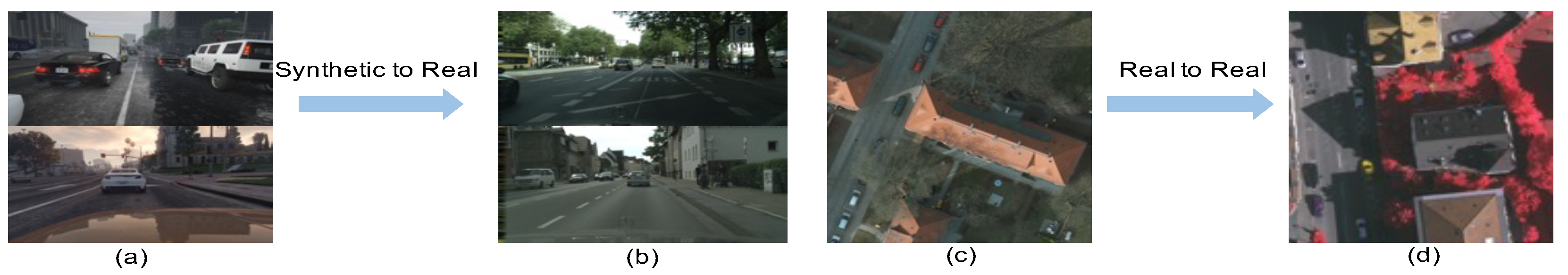
Second, underutilizing the feature of real-to-real translation of RS images (Figure 1). CycleGAN or DualGAN and many other image-to-image translation networks were initially designed to carry out not only real-to-real translation but also synthetic-to-real translation—such as photos to paints or game to the real world—while RS images translation is always real-to-real, where both sides are real-world images that are geographically significant. Synthetic-to-real translation is likely to bring a structure information change to a certain object because of the architecture of generators, which disturbs the task of segmentation. In addition, the gap of the marginal distribution between synthetic and real is larger than that between real and real, such as generating a Cityscapes [34] stylized image from GTA5 [35] where the generator is too overloaded to generate a new image, which could be largely avoided in RS images translation because both sides are from the real world.

Aimed at the two aforementioned problems, this paper proposes a new architecture of GANs based on DualGAN, named ResiDualGAN, for RS images domain translation and cross-domain semantic segmentation. ResiDualGAN resolves the first problem by using an in-network resizer module to fully utilize the scale information of RS images. Further, a residual connection that transfers the function of the generator from generating new images to generating residual items is used, which addresses the second problem. By simply combining with other methods, our proposed method reaches state-of-the-art accuracy performance in a common dataset. The main contributions of the paper can be summarized as follows:

1.

A new architecture of GANs, ResiDualGAN, is implemented based on DualGAN to carry out unpaired RS images cross-domain translation and cross-domain semantic segmentation tasks, in which an in-network resizer module and a residual architecture are used to fully utilize unique features of RS images compared with images used in the CV field. The experiment results show the superiority and stability of the ResiDualGAN. Our source code is available at https://github.com/miemieyanga/ResiDualGAN-DRDG (accessed on 12 January 2023).

2.

To the best of our knowledge, the proposed method reaches state-of-the-art performance when carrying out a cross-domain semantic segmentation task between two open-source datasets: Potsdam and Vaihingen [36]. The mIoU and F1-score are 55.83% and 68.04%, respectively, when carrying out a segmentation task from PotsdamIRRG to Vaihingen, showing increases of 11.71% and 11.09% compared with state-of-the-art methodologies.

3.

On the foundation of thorough experiments and analyses, this paper attempts to explain the reason why such great improvement could be achieved by implementing this kind of simple modification, which should be specially noted when a method from the CV field is applied to RS images processing.

2. Method

To describe the proposed methodology more specifically, some notions used in this paper should be defined first. Let $X_S\in {\mathbb{R}}^{H_S\times W_S\times B}$ be images from the source domain S with a resolution of $r_S$, where B is the number of channels. Let $X_T\in {\mathbb{R}}^{H_T\times W_T\times B}$ be images from the target domain T, with resolution $r_T$. $Y_S\in {\mathbb{Z}}^{H_S\times W_S\times C}$ are the labels of $X_S$, where C is the number of classes, while there are no labels for $X_T$. For simplifying the problem, we propose the following formulation. The size and resolution of images should conform to this formulation to diminish the effect of the scale factor:

$$\frac{H_S}{H_T}=\frac{W_S}{W_T}=\frac{r_T}{r_S}$$

(1)

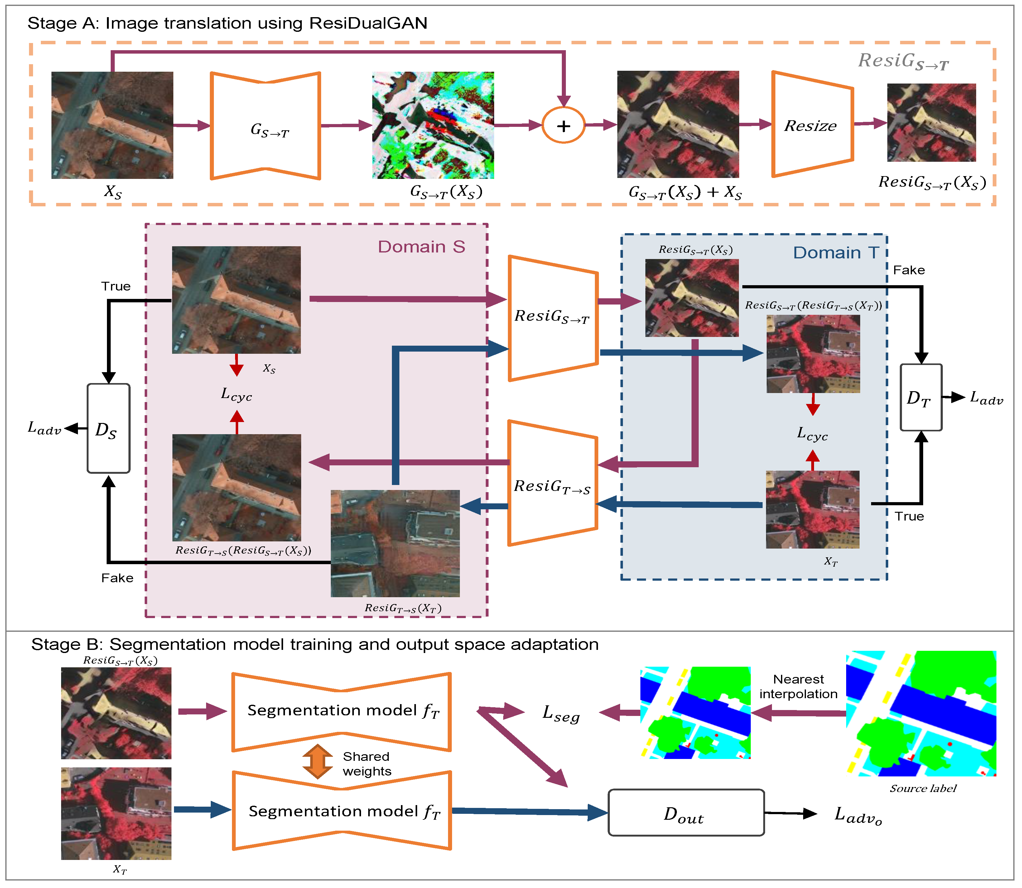
The objective of the proposed methodology is, for any given images $X_T$ in the target domain, we want to find a semantic segmentation model $f_T:X_T\to Y_T\in {\mathbb{Z}}^{H_T\times W_T\times C}$, which is expected to generate prediction labels $Y_T$ for $X_T$. The overview of the proposed method is shown in Figure 2, where two separated stages are implemented. Stage A is used to carry out an unpaired images style transfer from S to T with ResiDualGAN, which is proposed in this paper. Stage B trains a semantic segmentation model $f_T$ by utilizing the style-transferred images obtained from stage A with their respective labels $Y_S$. Additionally, an output space adaptation (OSA), proposed by [18], is applied during stage B, which is a more effective way to improve the performance of cross-domain semantic segmentation models compared with the feature-level adaptation used in many RS studies [27].

2.1. Stage A: Image Translation Using ResiDualGAN

2.1.1. Overall

The objective of Stage A is to translate $X_S$ to the style of $X_T$. Inspired by DualGAN [33], which is proven to be the optimal choice for VHR RS images translation [12], ResiDualGAN is proposed for VHR RS images translation, which consists of two major components: ResiGenerators and discriminators. ResiGenerator is exploited to generate a style-transferred image while the discriminator is designed to discern whether an image is generated by ResiGenerator or not. ResiDualGAN consists of two ResiGenerators, $Resi{G}_{S\to T}$ and $Resi{G}_{T\to S}$, and two discriminators, $D_S$ and $D_T$. $Resi{G}_{S\to T}$ is used for translating images from S to T, while $Resi{G}_{T\to S}$ is for T to S. $D_S$ performs the task of discerning whether an image is from S or being generated by $Resi{G}_{T\to S}$, while $D_T$ discerns whether an image is from T or being generated by $Resi{G}_{S\to T}$.

2.1.2. ResiGenerator

The architecture of $Resi{G}_{S\to T}:{\mathbb{R}}^{H_S\times W_S\times B}\to {\mathbb{R}}^{H_T\times W_T\times B}$ is illustrated in Figure 2, containing a generator $G_{S\to T}$ based on U-Net [4] and a resizer module $Resiz{e}_{S\to T}$. $G_{S\to T}:{\mathbb{R}}^{H_S\times W_S\times B}\to {\mathbb{R}}^{H_S\times W_S\times B}$ generates a residual item for its input. $Resiz{e}_{S\to T}:$${\mathbb{R}}^{H_S\times W_S\times B}\to {\mathbb{R}}^{H_T\times W_T\times B}$ is a resizing function that resizes images of the source domain to the size of the target domain, implemented as a network or an interpolation function. Based on ablation experiments discussed later in the paper, a bilinear interpolation function is used as the resizing function eventually. For the source domain images $X_S$, we want to obtain their corresponding target-stylized images $X_{S\to T}$ using $Resi{G}_{S\to T}$, which can be written as the following formulation:

$$X_{S\to T}=Resi{G}_{S\to T}\left(X_S\right)=Resiz{e}_{S\to T}\left(G_{S\to T}\left(X_S\right)+k\times X_S\right)$$

(2)

where k is the hyperparameter. All of the random noises are simplified for facilitating expression. According to the hypothesis in Equation (1), after the resizing operation, the resolution of $X_{S\to T}$ should be the same as $X_T$. The architecture of $Resi{G}_{T\to S}$ resembles $Resi{G}_{S\to T}$, where the only remaining difference is the resizer module $Resiz{e}_{T\to S}:{\mathbb{R}}^{H_T\times W_T\times B}\to {\mathbb{R}}^{H_S\times W_S\times B}$. $Resiz{e}_{T\to S}$ is a reverse procedure of $Resiz{e}_{S\to T}$, which resizes an image with the size of $H_T\times W_T\times B$ to the size of $H_S\times W_S\times B$. Consequently, the size and resolution of $Resi{G}_{T\to S}\left(X_{S\to T}\right)$ should be the same as $X_S$.

Our method is distinct from the super-resolution method. The super-resolution method only changes the resolution of images, while the aim of our paper is to minimize the domain gap between the source domain and the target domain. In fact, we can simply resize images to the same resolution and obtain a perfect super-resolution result. However, as shown in Section 4.3, the in-network resizer module performs better compared with the pre-resizing operation.

ResiGenerator is the main innovation of the proposed method. In general, we simply add an in-network resizer module and a residual connection into the original generator of DualGAN. However, in Section 3.4, we will evaluate that this simple modification leads to a significant improvement in performance. Further, in Section 4.3, we will demonstrate that only the combination of the in-network resizer module and the residual connection will bring such an improvement. If only the in-network resizer module or only the residual connection is used, the improvement will be quite limited.

2.1.3. Adversarial Loss

The ResiGenerator attempts to generate images to deceive the discriminator, while the discriminator attempts to distinguish whether images are generated by ResiGenerator or not, resulting in an adversarial loss $L_{adv}$. Analogous with DualGAN, a Wasserstein-GAN (WGAN) loss proposed by [37] is used to measure the adversarial loss. WGAN resolves the problem that the distance may be equal to 0 when there is no intersection of two data distributions by utilizing the Earth-Mover (EM) distance as a measure for two data distributions, which avoids the vanishing gradients problem of networks. Differentiate with traditional GANs [23], using a sigmoid output as a final output for the discriminator; discriminators of DualGAN remove the sigmoid as a final layer, which is also used by this paper. Moreover, the gradient penalty proposed by [38] is used to stabilize the training procedure and avoid the weights clipping operation in WGAN, which is in order to enforce the Lipschitz constraint in WGAN. The gradient penalty is not written in the formulations for the purpose of simplification. Above all, the adversarial loss $L_{adv}$ of source domain S to target domain T can be written as follows:

$$L_{adv}^{S\to T}={\mathbb{E}}_{x_T\sim X_T}\left(D_T\left(x_T\right)\right)-{\mathbb{E}}_{x_S\sim X_S}\left(D_T\left({ResiG}_{S\to T}\left(x_S\right)\right)\right)$$

(3)

2.1.4. Reconstruction Loss

$Resi{G}_{T\to S}$ reconstructs $X_{S\to T}$ to the style of the source domain. Ideally, $Resi{G}_{T\to S}\left(X_{S\to T}\right)$ should be entirely the same as $X_S$. However, loss always exists. Considering both sides of ResiDualGAN, the reconstruction loss $L_{cyc}$ can be measured by an L1 penalty as follows:

$$\begin{array}{cc}\hfill & L_{cyc}={\mathbb{E}}_{x_S\sim X_S}(\parallel Resi{G}_{T\to S}(Resi{G}_{S\to T}\left(x_S\right))-x_S{\parallel }_1)\hfill \\ \hfill & +{\mathbb{E}}_{x_T\sim X_T}(\parallel Resi{G}_{S\to T}\left(Resi{G}_{T\to S}\left(x_T\right)\right)-x_T{\parallel }_1)\hfill \end{array}$$

(4)

2.1.5. Total Loss

Considering adversarial loss and reconstruction loss together, the total loss for ResiDualGAN can be written:

$$\begin{array}{c}\hfill L_{ResiG}={\lambda }_{cyc}{L}_{cyc}+{\lambda }_{adv}(L_{adv}^{S\to T}+L_{adv}^{T\to S})\end{array}$$

(5)

where ${\lambda }_{cyc}$ and ${\lambda }_{adv}$ are hyperparameters corresponding to the reconstruction loss and the adversarial loss, respectively. During the training of ResiDualGAN, the discriminators attempts to maximize $L_{ResiG}$ while the ResiGenerator attempts to minimize, which can be written as the following min–max criterion:

$$\begin{array}{ccc}max& min& L_{ResiG}\\ D_S& Resi{G}_{S\to T}& \\ D_T& Resi{G}_{T\to S}& \end{array}$$

(6)

After the training of Stage A, a ResiGenerator $Resi{G}_{S\to T}$ can be obtained to perform the style translation task in Equation (2) and $X_{S\to T}$ is generated for the next training in Stage B, which is uncoupled with the training of Stage A.

2.2. Stage B: Segmentation Model Training

2.2.1. Overall

The objective of Stage B is to find the optimal model $f_T$ for semantic segmentation in the target domain (Figure 2, Stage B). In Stage B, an OSA is performed where we can regard $f_T$ as a generator in traditional GANs, which generates softmax prediction outputs for both $X_{S\to T}$ and $X_T$. Meanwhile, the function of discriminator $D_{out}$ in Stage B is to discern whether the output of $f_T$ is generated by $X_{S\to T}$ or $X_T$. OSA assumes that while images may be very different in appearance, their outputs are structured and share many similarities, such as spatial layout and local context. In this task, OSA minimizes the output space gap between $f_T\left(X_{S\to T}\right)$ and $f_T\left(X_T\right)$, and significantly improves the segmentation accuracy on $X_T$. As well as the traditional GANs, at the beginning, we will train $D_{out}$ firstly, followed by $f_T$.

2.2.2. Discriminator Training

Generally, because the semantic segmentation model is trained on the annotated source domain, the segmentation results of the source domain are more regular than those of target domain images. For example, the periphery of the building is clear for source domain images but zigzags for target domain images. OSA uses a discriminator $D_{out}$ to distinguish whether the segmentation result is from the source domain or the target domain, which encourages the model to generate regular results for target domain images. As a result, the segmentation results of the target domain are better both qualitatively and quantitatively after OSA. A binary cross-entropy loss $L_{out}$ is used for training $D_{out}$.

$$L_{out}=-{\mathbb{E}}_{x_T\sim X_T}\left(log(1-D_{out}\left(f_T\left(x_T\right)\right))\right)-{\mathbb{E}}_{x_{S\to T}\sim X_{S\to T}}\left(log\left(D_{out}\left(f_T\left(x_{S\to T}\right)\right)\right)\right)$$

(7)

2.2.3. Semantic Segmentation Training

At first, a cross-entropy loss is used to train $f_T$. Because the shape of $X_{S\to T}$ is $H_T\times W_T\times B$, while the shape of the label $Y_S$ is $H_S\times W_S\times C$, a nearest interpolation method is performed to resize $Y_S$ as $Y_{S\to T}\in {\mathbb{Z}}^{H_T\times W_T\times B}$. Then, the segmentation loss is

$$L_{seg}=-{\mathbb{E}}_{(x_{S\to T},y_{S\to T})\sim (X_{S\to T},Y_{S\to T})}(\sum _C^{c=1}{y}_{S\to T}log\left(f_T\left(x_{S\to T}\right)\right))$$

(8)

where $y_{S\to T}\in Y_{S\to T}$ is the nearest interpolation resizing of $y_S$, which is the label for $x_S\to T$. Next, we forward $X_T$ to $f_T$ and obtain an output $f_T\left(X_T\right)$, which attempts to fool the discriminator $D_{out}$, resulting in an adversarial loss $L_{ad{v}_o}$:

$$\begin{array}{c}\hfill L_{ad{v}_o}={\mathbb{E}}_{x_T\sim X_T}\left(log(1-D_{out}\left(f_T\left(x_T\right)\right))\right)\end{array}$$

(9)

2.2.4. Total Loss

Considering all items in Stage B, the total loss for the semantic segmentation task can be written as

$$\begin{array}{c}\hfill L_{total}={\lambda }_{seg}{L}_{seg}+{\lambda }_{ad{v}_o}{L}_{ad{v}_o}\end{array}$$

(10)

where ${\lambda }_{seg}$ and $L_{ad{v}_o}$ are hyperparameters corresponding to the segmentation loss and the the OSA loss. During the training of Stage B, we optimize the following min–max criterion:

$$\begin{array}{c}\hfill \underset{D_{out}}{max}\underset{f_T}{min}{L}_{total}\end{array}$$

(11)

After the training of Stage B, a semantic segmentation model $f_T$ for target images $X_T$ can be finally obtained.

2.3. Networks Settings

2.3.1. ResiGenerators

A ResiGenerator consists of a generator and an in-network resizer module. The generator is implemented as a U-Net [4], which is a fully convolutional network with skip connections between the down-sampling and up-sampling layers. For the down-sampling layers, we set the size of the convolving kernel as 4, padding as 1, and strides as 2. The channels of layers are {64, 128, 256, 512, 512, 512, 512}, where, except for the first layer and the final layer, all layers are followed by an instance normalization [39] and a Leaky ReLU [40] with a negative slope of 0.2. For up-sampling layers, the same convolving kernel size, stride, and padding values from the down-sampling layers are utilized. All layers are composed of a transposed convolutional layer followed by an instance normalization and a ReLU [41]. Dropout layers with a probability of 0.5 are exploited in all up-sampling and down-sampling layers with more than 256 channels. The resizer module could be implemented in many approaches. Based on the experimental results in Section 4.3.2, we eventually exploit the bilinear interpolation as the optimal implementation of the resizer module.

2.3.2. Discriminators

Discriminators of ResiDualGAN are implemented as fully convolutional networks as well. The channels of layers are {64, 128, 256, 512, 512, 1}, where, except for the last layer, all the layers are followed by a batch normalization [42] layer and a Leaky ReLU with a negative slope of 0.2. The output of the last layer does not pass through any activation functions due to the constraints of WGAN [37].

2.3.3. Output Space Discriminator

The implementation is totally the same as that in [18], which is a fully convolutional network with a kernel of 4 × 4; stride of 2; and channels of 64, 128, 256, 512, 1. Except for the last layer, every layer is followed by Leaky ReLU with a negative slope of 0.2. The output of the last layer is resized to the size of the input.

2.3.4. Segmentation Baseline

DeeplabV3 [43] is adopted as the baseline network for the semantic segmentation task of the proposed method. To accelerate the coverage procedure, the encoder of the baseline is replaced with ResNet-34 [44], which is pre-trained on ImageNet [45].

2.4. Training Settings

All the models are implemented on PyTorch 1.8.1 and trained on an NVIDIA A30 with 24 GB RAM running Ubuntu 18.04. The total time consumption is about 23 h, where 80% of the time is used for training ResiDualGAN and the remaining 20% is for the segmentation model and output space adaptation. The total time consumption is approximate to that of DualGAN [33] and CycleGAN [24], and is more efficient than MUCSS [12] (about 30 h), which needs to generate pseudo labels and perform self-training.

2.4.1. Stage A

We set $k=1$, ${\lambda }_{adv}=1$, and ${\lambda }_{cycle}=10$ for training of the ResiDualGAN. Adam [46] with $\beta =\left(0.5,0.999\right)$ is adopted as the optimizer for ResiGenerators, while RMSProp [47] with $\alpha =0.99$ is adopted for the discriminators. The learning rates for all ResiGenerators and discriminators are set as 0.0005. The batch size is set as 1, where we randomly select images from the source domain and the target domain for training. For every 5 iterations of training for discriminators, 1 iteration of training for ResiGenerators is performed. Finally, a total of 100 epochs are trained.

2.4.2. Stage B

We set ${\lambda }_{seg}=1$ and $L_{ad{v}_o}=0.02$ for the training of Stage B. Adam with $\beta =(0.9,0.999)$ is adopted as the optimizer for semantic segmentation model $f_T$ and output space discriminator $D_{out}$. The initial learning rates are both set as 0.0002. We dynamically adjust the learning rate of $f_T$ by multiplying by 0.5 when the metrics have stopped ascending. The batch size is set as 16.

3. Experimental Results

3.1. Datasets

To fully verify the effectiveness of the proposed UDA method, three VHR RS datasets are introduced in the experiment, namely, the Potsdam dataset, Vaihingen dataset, and BC403 dataset.

The first two datasets belong to the ISPRS 2D open-source RS semantic segmentation benchmark dataset [36]; all images are processed into true orthophotos (TOPs), with annotations of 6 ground classes: clutter/background, impervious surface, car, tree, low vegetation, and building. The Potsdam dataset contains three different band modes: IR-R-G (three channels), R-G-B (three channels), and IR-R-G-B (four channels). IR-R-G and R-G-B are exploited in the following experiments and are abbreviated as PotsdamIRRG and PotsdamRGB. Both datasets consist of 38 VHR TOPs with a fixed size of 6000 × 6000 pixels and spatial resolution of 5 cm. The Vaihingen dataset contains only one band mode, IR-R-G (three channels), and consists of 33 TOPs, in which every TOP contains 2000 × 2000 pixels with a resolution of 9 cm. To conform to the constraints of Equation (1), we clip images of Potsdam into the size of 896 × 896 and images of Vaihingen into the size of 512 × 512, where the numbers 896 and 512 are specifically set for facilitating the down-sampling operation in the CNN. Eventually, 1296 images for PotsdamIRRG and PotsdanRGB, and 1696 images for Vaihingen—in which 440 images of Vaihingen are validation datasets—are obtained.

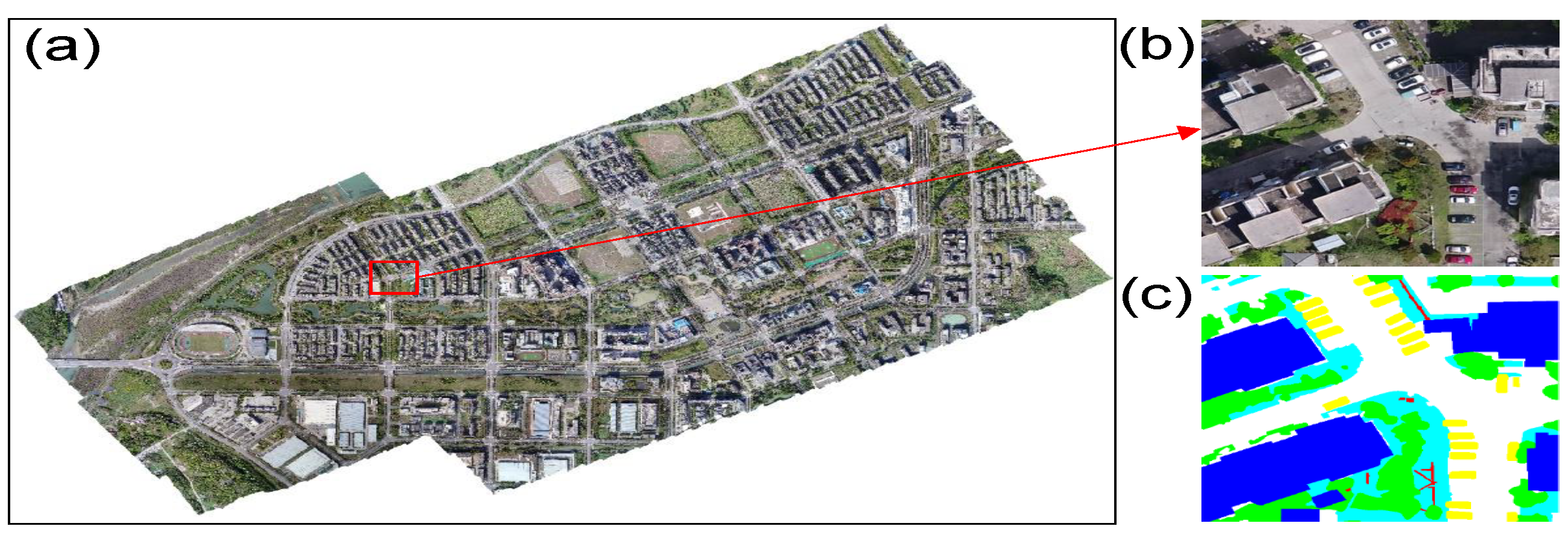
The third dataset (BC403) is manually annotated by us. This dataset is constructed using VHR drone imagery obtained from Beichuan County area with a spatial resolution of 7 cm. Beichuan County is located in southwestern China, under the jurisdiction of Mianyang City, Sichuan Province. This dataset was collected in April 2018 and is part of the Wenchuan Earthquake 10th Anniversary UAV dataset. Beichuan County has a subtropical monsoonal humid climate and has architectural features typical of Chinese counties, which is totally different from the above two datasets in terms of image feature characteristics. The original image size of the dataset is 27,953 × 43,147 (Figure 3a). The down-sampled RS images are cropped into 1584 tiles of 768 × 768 pixels with 30% overlapping (Figure 3b). Images in this dataset are provided with their semantic labels (Figure 3c), including six classes of ground objects—clutter/background, impervious surface, car, tree, low vegetation, and building—as in the Potsdam and Vaihingen dataset. We select 20% of the images as the validation dataset and the remaining images for the test dataset. The test dataset does not overlap with the validation dataset.

3.2. Experimental Settings

We design three cross-domain tasks to simulate situations that might be encountered in practical applications using the above datasets:

1.

IR-R-G to IR-R-G: PotsdamIRRG to Vaihingen. A commonly used benchmark for evaluating models.

2.

R-G-B to IR-R-G: PotsdamRGB to Vaihingen. Another commonly used benchmark for evaluating models.

3.

IR-R-G to RGB: PotsdamIRRG to BC403. Instead of using PotsdamRGB as the target dataset, where channels of R and G are identical with PotsdamIRRG, we use our annotated BC403 dataset to perform this cross-domain task.

3.3. Evaluation Metrics

To facilitate comparison with different methods, IoU and F1-score are employed as metrics in this paper. For every class in six different ground classes, the formulation of IoU can be written as

$$\mathrm{IoU}=\frac{\left|\mathrm{A}\cap \mathrm{B}\right|}{\left|\mathrm{A}\cup \mathrm{B}\right|}$$

(12)

where A is the ground truth and B denotes the predictions. After calculations of IoU for six classes, mIoU can be obtained, which is the mean IoU for every class. The F1-score can be written as

$$\mathrm{F}1-\mathrm{score}=\frac{2\times \mathrm{Precision}\times \mathrm{Recall}}{\mathrm{Precision}+\mathrm{Recall}}$$

(13)

3.4. Compared with the State-of-the-Art Methods

For a comprehensive comparative analysis, we keep all of the settings of networks consistent with ours and hyperparameters in other methods as optimal as possible. Four state-of-the-art methods are used for comparison, i.e., Benjdira’s [26], DualGAN [33], AdaptSegNet [18], and MUCSS [12], where the former two are image-to-image translation methods, AdaptSegNet is an adversarial discriminative method, and MUCSS combines DualGAN with self-training strategies for cross-domain semantic segmentation tasks.

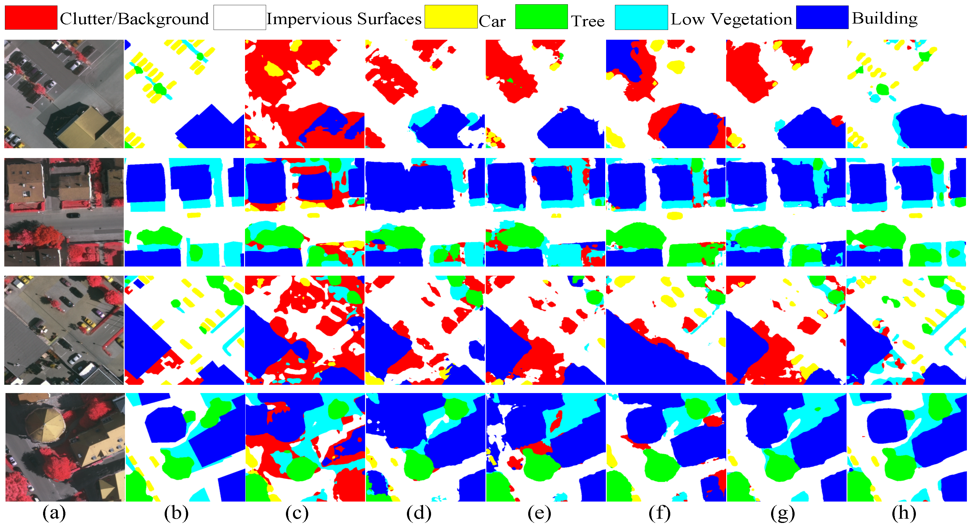
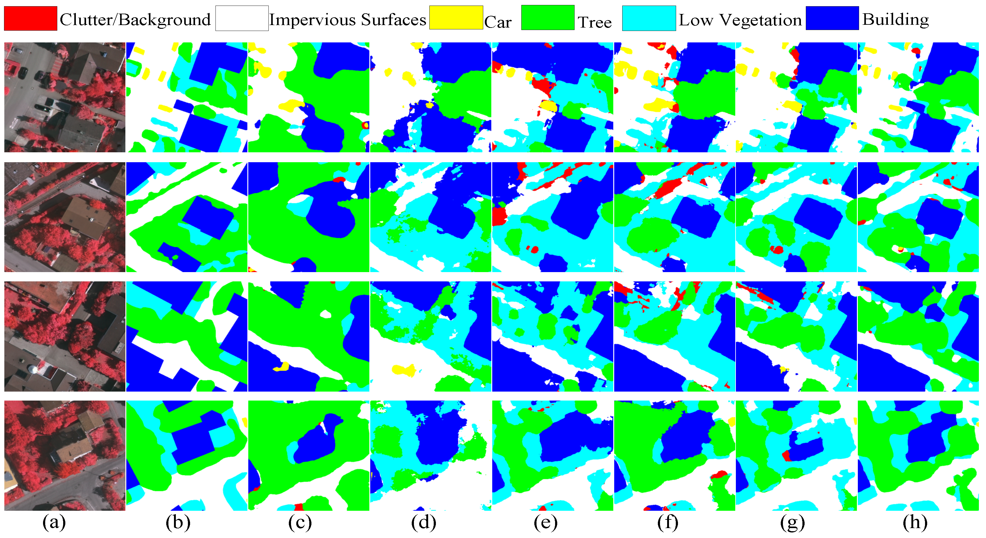
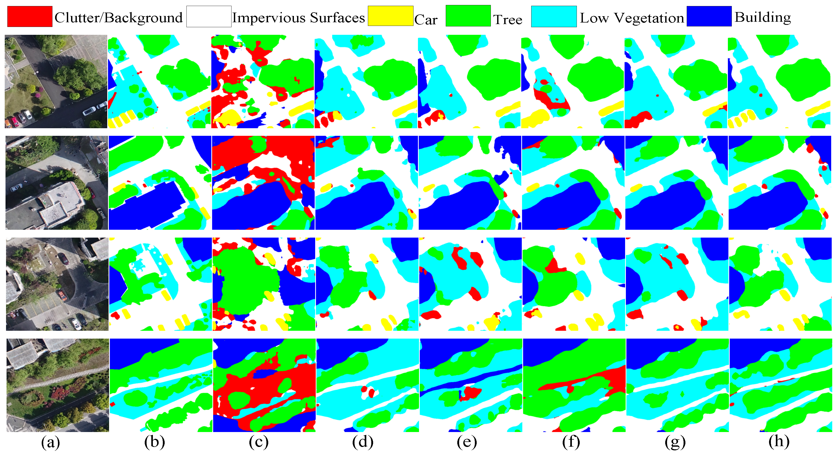
Both the quantitative and qualitative results show the superiority of the proposed methods.

Table 1. The quantitative results of the cross-domain semantic segmentation from PotsdamIRRG to Vaihingen.

Methods	Background/Clutter		Impervious Surface		Car		Tree		Low Vegetation		Building		Overall
	IoU	F1Score	IoU	F1Score	IoU	F1Score	IoU	F1Score	IoU	F1Score	IoU	F1Score	IoU	F1Score
Baseline (DeeplabV3 [43])	2.12	4.01	47.68	64.47	20.39	33.62	51.37	67.81	30.25	46.38	65.74	79.28	36.26	49.26
Benjdira’s [26]	6.93	9.95	57.41	72.67	20.74	33.46	44.31	61.08	35.60	52.17	65.71	79.12	38.45	51.41
DualGAN [33]	7.70	11.12	57.98	73.04	25.20	39.43	46.12	62.79	33.77	50.00	64.24	78.02	39.17	52.40
AdaptSegNet [18]	5.84	9.01	62.81	76.88	29.43	44.83	55.84	71.45	40.16	56.87	70.64	82.66	44.12	56.95
MUCSS [12]	10.82	14.35	65.81	79.03	26.19	40.67	50.60	66.88	39.73	56.39	69.16	81.58	43.72	56.48
ResiDualGAN	8.20	13.71	68.15	81.03	49.50	66.06	61.37	76.03	40.82	57.86	75.50	86.02	50.59	63.45
ResiDualGAN + OSA	11.64	18.42	72.29	83.89	57.01	72.51	63.81	77.88	49.69	66.29	80.57	89.23	55.83	68.04

The bold number is the best result of every column.

and Figure 4 show the quantitative and qualitative segmentation results of PotsdamIRRG to Vaihingen, respectively;

Table 2. The quantitative results of the cross-domain semantic segmentation from PotsdamRGB to Vaihingen.

Methods	Background/Clutter		Impervious Surface		Car		Tree		Low Vegetation		Building		Overall
	IoU	F1Score	IoU	F1Score	IoU	F1Score	IoU	F1Score	IoU	F1Score	IoU	F1Score	IoU	F1Score
Baseline ((DeeplabV3 [43])	1.81	3.43	46.29	63.17	13.53	23.70	40.23	57.27	14.57	25.39	60.78	75.56	29.53	41.42
Benjdira’s [26]	2.03	3.14	48.48	64.99	25.99	40.57	41.97	58.87	23.33	37.50	64.53	78.26	34.39	47.22
DualGAN [33]	3.97	6.67	49.94	66.23	20.61	33.18	42.08	58.87	27.98	43.40	62.03	76.35	34.44	47.45
AdaptSegNet [18]	6.49	9.82	55.70	71.24	33.85	50.05	47.72	64.31	22.86	36.75	65.70	79.15	38.72	51.89
MUCSS [12]	8.78	12.78	57.85	73.04	16.11	26.65	38.20	54.87	34.43	50.89	71.91	83.56	37.88	50.30
ResiDualGAN	8.80	13.90	52.01	68.35	42.58	59.58	59.88	74.87	31.42	47.69	69.61	82.04	44.05	57.74
ResiDualGAN +OSA	9.76	16.08	55.54	71.36	48.49	65.19	57.79	73.21	29.15	44.97	78.97	88.23	46.62	59.84

The bold number is the best result of every column.

and Figure 5 are PotsdamRGB to Vaihingen; and

Table 3. The quantitative results of the cross-domain semantic segmentation from PotsdamIRRG to BC403.

Methods	Background/Clutter		Impervious Surface		Car		Tree		Low Vegetation		Building		Overall
	IoU	F1Score	IoU	F1Score	IoU	F1Score	IoU	F1Score	IoU	F1Score	IoU	F1Score	IoU	F1Score
Baseline (DeeplabV3 [43])	2.74	5.26	27.35	42.44	35.68	52.22	43.18	60.02	11.43	19.99	60.51	75.20	30.15	42.52
Benjdira’s [26]	4.79	6.54	68.37	79.65	47.99	54.76	22.69	45.76	22.68	42.05	72.57	80.85	39.85	51.60
DualGAN [33]	3.52	8.78	66.48	80.97	39.26	64.35	30.58	36.68	28.03	35.73	68.53	83.63	39.40	51.69
AdaptSegNet [18]	4.57	8.17	56.37	72.03	50.90	66.95	52.01	67.87	14.70	25.06	74.38	85.17	42.15	54.21
MUCSS [12]	3.13	5.86	71.83	83.35	27.72	41.62	32.53	48.17	27.95	42.08	78.82	87.82	40.33	51.48
ResiDualGAN	13.79	23.72	72.26	83.64	61.06	75.69	46.56	62.76	33.73	49.67	76.08	86.15	50.58	63.61
ResiDualGAN + OSA	13.25	23.03	75.51	85.95	61.32	75.87	51.22	67.18	35.35	51.33	82.51	90.24	53.19	65.60

The bold number is the best result of every column.

and Figure 6 are PotsdamIRRG to BC403. After the OSA, we finally obtain the mIoU and F1-score of segmentation results of 55.83% and 68.04% from PotsdamIRRG to Vaihingen, an increase of 11.71% and 11.09%, respectively, compared with other methods; for PotsdamRGB to Vaihingen, we obtain 46.62% and 59.84%, an increase of 7.90% and 7.95%; for PotsdamIRRG to BC403, we obtain 53.19% and 65.60%, an increase of 11.04% and 11.39%. It can be observed that the improvement in car class is significant while the improvement in low vegetation is deficient. In Section 4.3.1, we will discuss the principal reason for these imbalanced improvements.

4. Discussion

4.1. Hyperparameters Settings

To boost the performance of our model, we evaluate the proposed method (ResiDualGAN+OSA) on the evaluation datasets of Vaihingen under the task of transferring the segmentation model from PotsdamIRRG to Vaihingen. The grid search method is used to find the optimal hyperparameters combination.

Table 4. Evaluation results of ResiDualGAN under different hyperparameter settings. The results are obtained from the task of cross-domain semantic segmentation from PotsdamIRRG to Vaihingen and evaluated on the validation part of Vaihingen. The mIoU and F1 are overall IoU and overall F1-score, respectively.

Hyperparameters Settings		mIoU	F1
$L_{adv},L_{cyc}=(1,10)$	$k=0.5$	53.29	66.09
	$k=1$	56.80	68.46
	$k=2$	55.10	67.39
$k=1$	$L_{adv},L_{cyc}=(1,1)$	56.00	68.24
	$L_{adv},L_{cyc}=(1,5)$	56.71	69.10
	$L_{adv},L_{cyc}=($1, 10)	56.80	68.46
	$L_{adv},L_{cyc}=(1,20)$	54.79	67.34
	$L_{adv},L_{cyc}=(5,1)$	54.43	67.33
	$L_{adv},L_{cyc}=(5,5)$	52.69	65.02
	$L_{adv},L_{cyc}=(5,10)$	55.73	68.26
	$L_{adv},L_{cyc}=(10,1)$	53.39	65.51
	$L_{adv},L_{cyc}=(10,5)$	55.12	67.10
	$L_{adv},L_{cyc}=(10,10)$	54.98	67.56

The bold number is the best result of every column.

shows the results of the grid search. Firstly, for a given $L_{adv},L_{cyc}=(1,10)$, we evaluate the model’s performance under different k settings. When $k=1$, the best result is reached with mIoU = 56.80% and and overall F1-score = 68.46%. Secondly, with $k=1$ fixed, we evaluate how the settings of $L_{adv},L_{cyc}$ affect the model’s performance. We split the grid of the search space into $\{1,5,10\}\times \{1,5,10\}$, where × is the Cartesian product. The best result is obtained when $L_{adv},L_{cyc}=(1,10)$. Eventually, we set the hyperparameters of ResiDualGAN as $k,L_{adv},L_{cyc}=(1,1,10)$.

In addition, we can observe that the results do not fluctuate too much under different hyperparameter settings (max of mIou − min of mIou = 56.80% − 52.69% = 4.11%), which demonstrates the stability of our model under different hyperparameter settings.

4.2. Image Translation

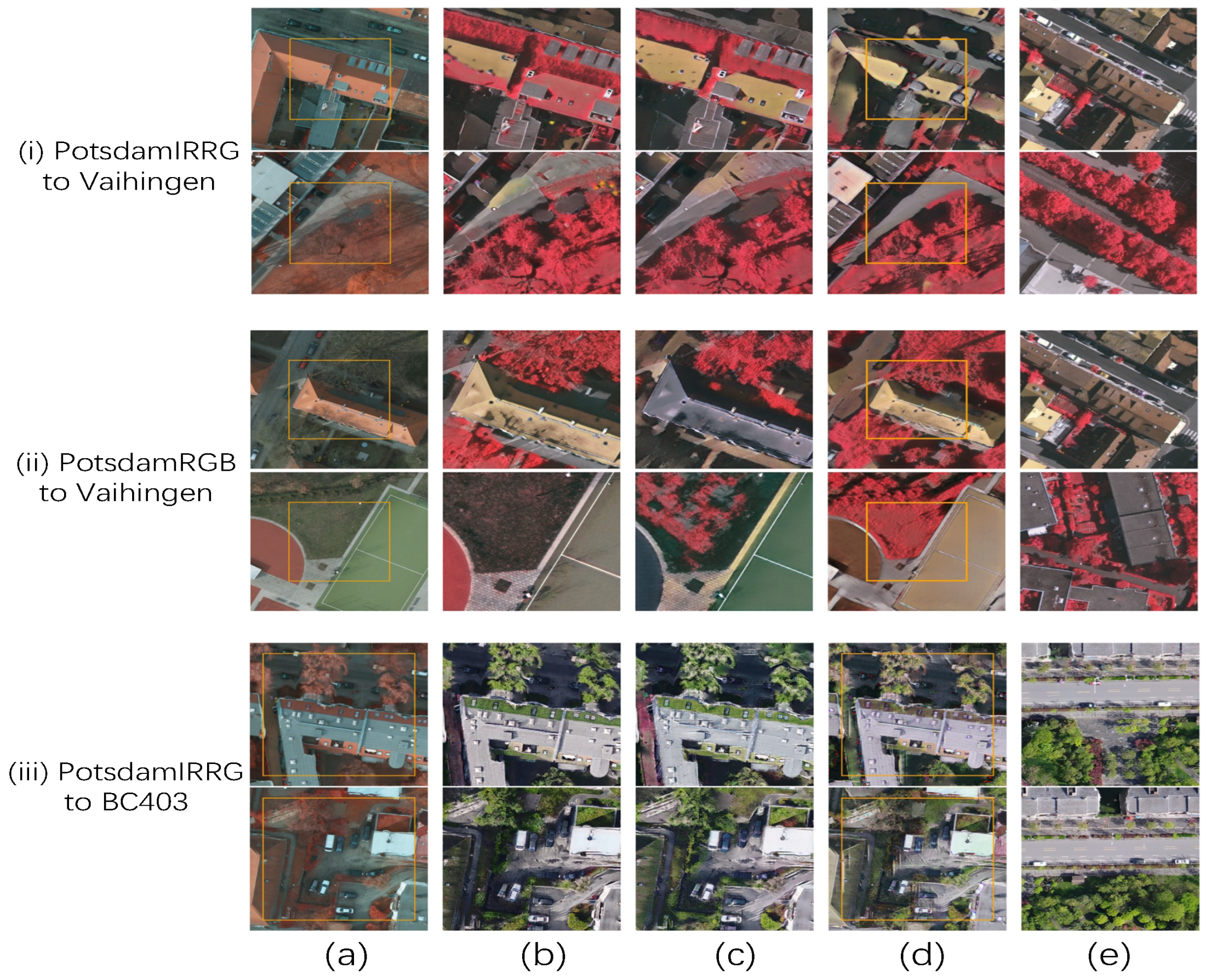
Figure 7 shows the image translation results of ResiDualGAN. The translation of the tan roof in Figure 7(i-a) is a tough problem for the existing GANs, where the tan roof is likely to be translated as low vegetation, e.g., Figure 7(i-b) and Figure 7(i-c). The ResiDualGAN avoids this problem, as shown in Figure 7(i-d), where the tan roof is translated into yellow, which corresponds to Vaihingen in Figure 7(i-e). Although great improvement has been made, the translated results of ResiDualGAN are still visually unfriendly; where the color of the imperious surface is translated into yellow, the shadow is too thick to recognize the objects below the shadow, and so on. Fortunately, although visually unfriendly, the translated results of ResiDualGAN are suitable for the training in Stage B. The state-of-the-art segmentation performance fully proves the superiority of ResiDualGAN in RS images’ cross-domain semantic segmentation tasks.

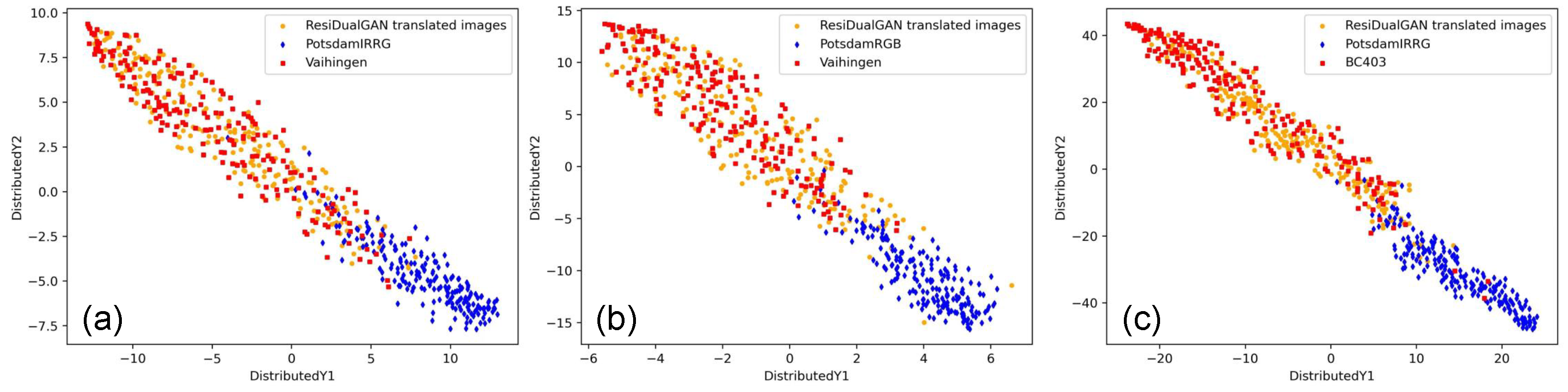
Figure 8 shows the t-SNE [48] visualized result of image translation. t-SNE stands for t-distributed stochastic neighbor embedding, which is a method for dimensionality reduction. t-SNE is a commonly used visualizing method to show the data distribution of different domains. In our paper, what we want to do is to show the data distribution of the source domain (e.g., PotsdamIRRG), target domain (e.g., Vaihingen), and ResiDualGAN-transferred images (e.g., transferred images from PotsdamIRRG to Vaihingen). To achieve this, we need to extract the semantic features of every image first. We train a classification network based on ResNet-18 [44]. The classification network is designed to distinguish whether an image is from the source domain (PotsdamIRRG) or the target domain (Vaihingen). After training the network roughly, we pass the source domain images (PotsdamIRRG), target domain images (Vaihingen), and ResiDualGAN-transferred images (transferred images from PotsdamIRRG to Vaihingen) through the encoder of the network and obtain the semantic features. Then, we use t-SNE to reduce the dimension of the semantic features to two. We draw every two-dimensional point in Figure 8. The visualization result shows that ResiDualGAN matches the data distribution of the source domain data with the target domain data well. The feature distribution of most of the translated images is similar to those of the target domain.

4.3. Ablation Study

4.3.1. Resizer Module

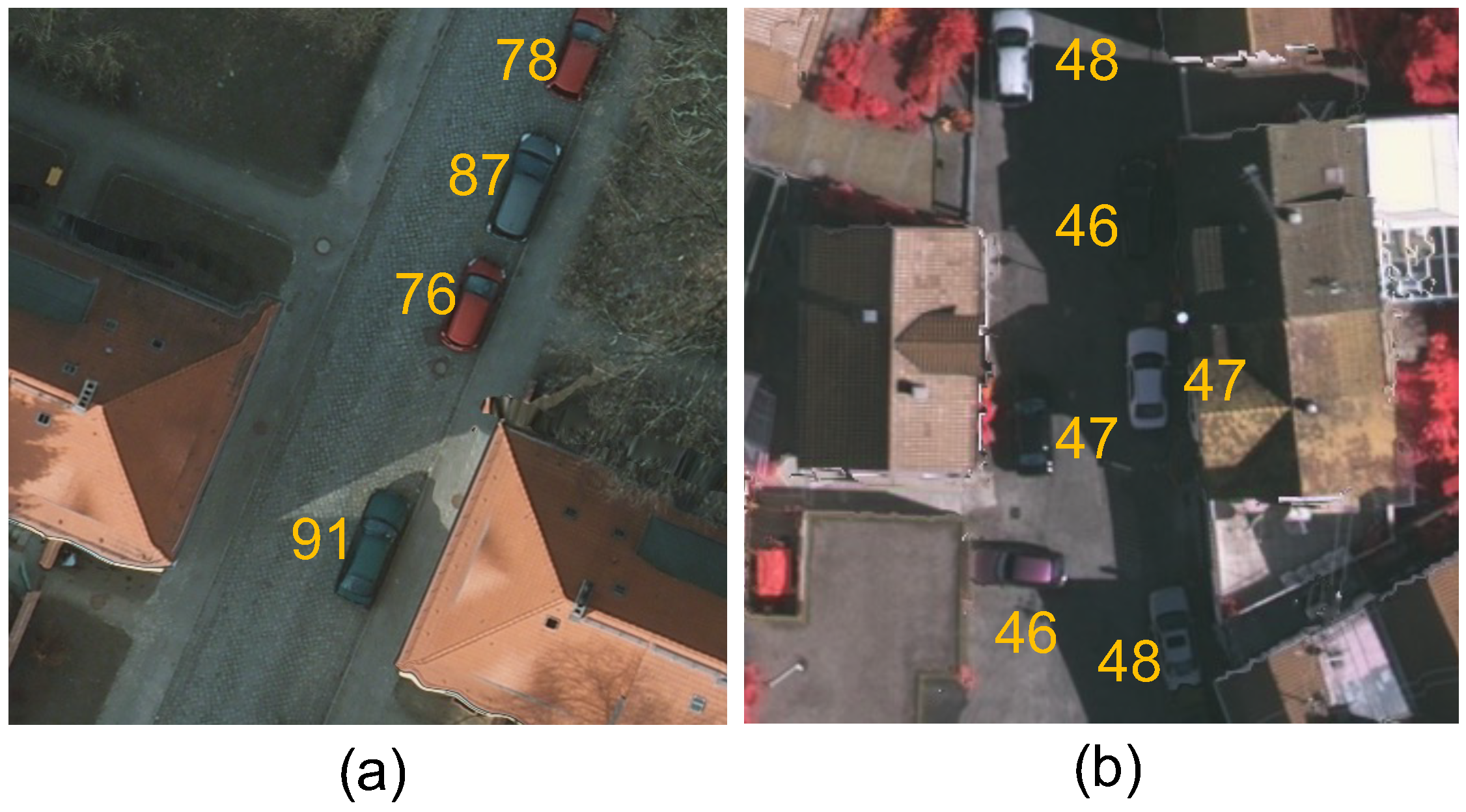
In RS images, some scale-invariant classes (e.g., cars) have a relatively fixed size because of the fixed resolution of RS images. Therefore, if two datasets have different resolutions, the size of cars may be distinct. Figure 9 shows that kind of tendency; the sizes of cars in PotsdamIRRG are close to each other but are always much larger than cars in Vaihingen.

CNN is a scale-sensitive network [49]. CNN learns to recognize features from the training data and predicts testing data using the knowledge learned from the training data. Consequently, for scale-invariant objects, e.g., cars, scale is a feature that can be learned for CNN. Scale-sensitivity of CNN brings a great challenge for some CV tasks, such as the detection of cars from street scene images [49,50], where cars in such images present a large variance in scale (as shown in Figure 1, cars in street scene images). However, the variance in scale benefits the UDA tasks. By learning different scale information of a category, CNN possesses the ability to recognize objects with different scales, which benefits the UDA semantic segmentation tasks of car, person, and other scale-invariant classes from GTA5 to Cityscapes. Nevertheless, as mentioned above, the sizes of scale-invariant classes in an RS dataset are close to each other, which greatly challenges the UDA tasks of RS images.

The resizer module in ResiDualGAN addresses the scale discrepancy problem of two domains. Complying with Equation (1), ResiDualGAN unifies the resolution of target domain images $X_T$ and $Resi{G}_{S\to T}\left(X_S\right)$ to $r_T$, and the resolution of source domain images $X_S$ and $Resi{G}_{T\to S}\left(X_T\right)$ to $r_S$, addressing the problem of both discriminators $D_S$ and $D_T$ receiving two images with different resolutions, which may avoid the vanishing gradient problem of discriminators and accelerate the convergence of generators.

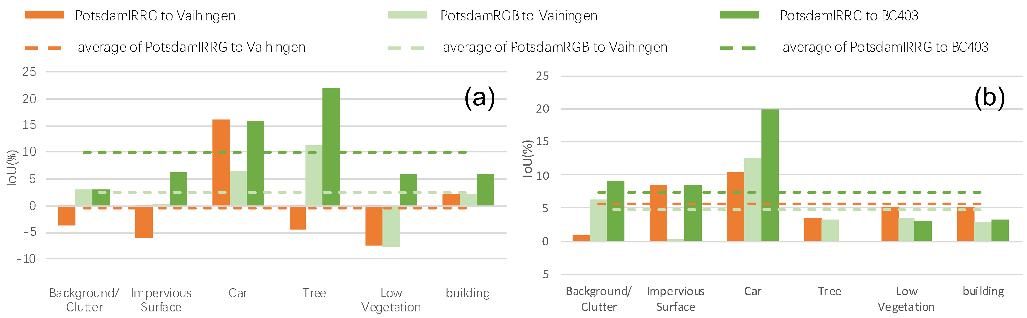
The resizer module greatly improves the accuracy performance of ResiDualGAN in cross-domain RS image semantic segmentation tasks. If we remove the resizer module, the mIoU drops to 44.97% and the F1-score drops to 58.51% (

Table 5. Ablation study for ResiDualGAN. The results are obtained from the task of cross-domain semantic segmentation (from PotsdamIRRG to Vaihingen) and evaluated on the test part of Vaihingen. The mIoU and F1 are overall IoU and overall F1-score, respectively.

Experiment	Method	mIoU	F1
Resize	No Resize	44.97	58.51
	Pre-resize	53.46	66.10
	In-network Resize	55.83	68.04
Resizing Function	Nearest	53.86	66.30
	Bilinear	55.83	68.04
	Resizer model	52.97	65.88
Backbone	ResNet [44]	52.51	65.33
	LinkNet [51]	52.22	64.84
	U-Net [4]	55.83	68.04
Residual Connection	No Residual	38.67	52.37
	Residual (fixed k)	55.83	68.04
k	Learnable	54.05	67.02
	Fixed	55.83	68.04

The bold number is the best result of every column.

). Figure 10 shows the improvements provided by the resizer module of ResiDualGAN under two pairs of comparisons: (1) DualGAN vs. ResiDualGAN (No Residual) and (2) ResiDualGAN (No Resizer) vs. ResiDualGAN. ResiDualGAN (No Residual) is just an extension of DualGAN that adds a resizer module after the generator, and ResiDualGAN (No Resizer) only removes the resizer module in ResiGenerator. We perform the experiments using the same hyperparameter settings. The results show that, for scale-invariant classes (e.g., cars), the improvements are much higher than the average, while for scale-invariant classes (e.g., low vegetation), the improvements are under the average.

Additionally, in-network resizing also affects the performance. Previous works [27,32] use the resizing function as a pre-processing step for input data, which leads to information loss. An in-network resizer module adapts itself while resizing images, bringing better performance. Table 5 shows the experimental results, in which a pre-processing resizing operation reduces the mIoU from 55.83% to 53.46% and the F1-score from 68.04% to 66.10%, which demonstrates the superiority of our method.

4.3.2. Resizing Function

Different image resizer methods may affect the on-task performance of networks [52]. Consequently, the implementation of the resizer module will have a significant effect on the semantic segmentation results. In this paper, we compare three types of resizing methods: nearest interpolation; bilinear interpolation; and a resizer model, which is proposed by [52]. The former two methods are linear methods that contain no parameters to be learned, and the last method is a lightweight network that has shown its superiority compared with linear methods on some CV tasks. Table 5 shows the experimental results for the optimal resizer module, where the bilinear interpolation obtains the highest mIoU and F1-score. The nearest interpolation obtains worse results compared with the bilinear interpolation, resulting from the information loss of images. The resizer model shows the worst results and should be further optimized to adapt the VHR RS images translation tasks better in future works. As a result, the bilinear interpolation method is selected as the implementation of the resizer module of ResiDualGAN.

4.3.3. Backbone

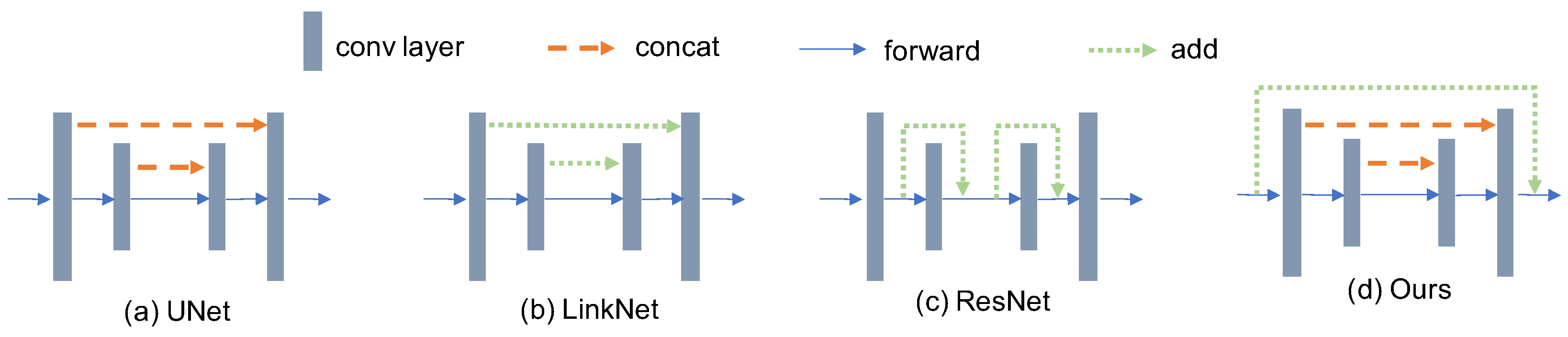
The setting of the backbone of the generator will affect the segmentation model’s accuracy. We quantitatively compare three CNN-based backbones: U-Net [4], LinkNet [51], and ResNet [44]. The structures of the three networks are shown in Figure 11. U-Net (Figure 11a) is a commonly used backbone in the generation tasks, which connects encoder and decoder layers with feature concatenation. LinkNet (Figure 11b) resembles U-Net but replaces the concat operation as a plus operation between layers. ResNet (Figure 11c) utilizes residual connections on a feature level that contribute to building a deeper network. In particular, it is worth noting that the residual connection of ResiDualGAN is totally distinct from it in ResNet. As Figure 11d shows, ResiDualGAN merely adds the input with the output of the backbone. In ResNet, the skip connection is used to add the input feature to the output feature, where the feature is firstly passed through the encoder and added to the feature with the same channels. The procedure of encoding an image to a feature map produces unnecessary information loss. The optimal way is to add the input image to the output image of the backbone, where the function of the backbone becomes generating a residual item but encoding an image and then decoding to obtain a new image. The experimental results are shown in Table 5. For a fair comparison, we control the parameters of the three backbones to be generally equivalent. The quantitative results illustrate that U-Net is the better choice as a backbone for our generative model. The experimental results also show that our residual connection design is much better.

4.3.4. Residual Connection

Combining with the resizer module, the residual connection plays a pivotal role in achieving the state-of-the-art accuracy performance of ResiDualGAN. If we remove the residual connection in our model, the mIoU drops from 55.83% to 38.67% and the overall F1-score drops from 68.04% to 52.37%, as shown in Table 5. The residual connection retains the original data and avoids the modification of the structure information. Translation between RS datasets is real-to-real, where all the pixels are geographically significant. Image-to-image translation GANs such as DualGAN are widely utilized in UDA, which not only perform real-to-real translation but also synthetic-to-real translation, e.g., GTA5 to Cityscapes. However, real-to-real translation is distinct from synthetic-to-real translation. Intuitively, during the procedure of image-to-image translation, the networks should modify the real images less than the synthetic images, where the margin distribution between real and real is more closed than between synthetic and real [53]. Meanwhile, it is not expected to modify the structure information of real images, which may affect the segmentation performance. Nevertheless, the U-shape network generator of DualGAN is likely to modify the structure information. The residual connection of ResiDualGAN retains the original structure information as much as possible and focuses on the translation of other information, e.g., color, shadow, and so on. As a result, the residual connection improves the segmentation performance and is more suitable for RS images translation.

4.3.5. Fixed k

k is a vital parameter for ResiDualGAN, which decides how much of the residual item will affect the generated image. Rather than giving a fixed number, we can also set the k as a learnable parameter and update k in every iteration. The experimental results in Table 5 show that the fixed $k=1$ reaches a better result.

4.4. Output Space Adaptation

An output space adaptation is adopted to further improve the performance of ResiDualGAN. Theoretically, different from image classification based on features that describe the global visual information of the image, high-dimensional features learned for semantic segmentation encode complex representations. As a result, adaptation in the feature space may not be the best choice for semantic segmentation [18]. The OSA has been proven to be more effective than feature space adaptation when facing the semantic segmentation task of RS images [27]. In this paper, the OSA improves the mIoU by 5.24% from PotsdamIRRG to Vaihingen, 2.57% from PotsdamRGB to Vaihingen, and 1.61% from PotsdamIRRG to BC403. The OSA can also be replaced with other methods, such as self-training, to reach higher accuracy performance in future works. A more thorough discussion of Stage B is beyond the scope of this paper.

5. Conclusions

With the aim to learn a semantic segmentation model for RS images from an annotated dataset to an unannotated dataset, ResiDualGAN has been proposed in this paper to minimize the domain gap at the pixel level. Considering the scale discrepancy of scale-invariant objects, an in-network resizer module is used, which greatly increases the segmentation accuracy of scale-invariant classes. Considering the feature of real-to-real translation of RS images, a simple but effective residual connection is utilized, which not only stabilizes the training procedure of the GANs model but also improves the accuracy of results when combined with the resizer module. Combined with an output space adaptation, we reach state-of-the-art accuracy performance on the benchmarks, which highlights the superiority and reliability of the proposed method.

ResiDualGAN is a simple, stable, and effective method to train an adversarial generative model for RS images cross-domain semantic segmentation tasks. However, ResiDualGAN only minimizes the pixel-level domain gap. How to combine ResiDualGAN with adversarial discriminative methods that minimize the feature-level and output-level domain gap and self-training strategies that are better for higher performance in cross-domain semantic segmentation of RS images is a potential topic for future works. In addition, the input image size of ResiDualGAN is strictly limited because of the constraints of the down-sampling process of CNN. Utilizing the Transformer [25] to replace all or part of the CNN components will be a further step of ResiDualGAN.

References

- Gao, H.; Guo, J.; Guo, P.; Chen, X. Classification of Very-High-Spatial-Resolution Aerial Images Based on Multiscale Features with Limited Semantic Information. Remote Sens. 2021, 13, 364. [Google Scholar] [CrossRef]
- Krizhevsky, A.; Sutskever, I.; Hinton, G.E. ImageNet Classification with Deep Convolutional Neural Networks. In Proceedings of the Advances in Neural Information Processing Systems, Lake Tahoe, NV, USA, 3–8 December 2012; Curran Associates, Inc.: Red Hook, NY, USA, 2012; Volume 25. [Google Scholar]
- Long, J.; Shelhamer, E.; Darrell, T. Fully convolutional networks for semantic segmentation. In Proceedings of the 2015 IEEE Conference on Computer Vision and Pattern Recognition (CVPR), Boston, MA, USA, 7–12 June 2015; pp. 3431–3440. [Google Scholar]
- Ronneberger, O.; Fischer, P.; Brox, T. U-net: Convolutional networks for biomedical image segmentation. In Medical Image Computing and Computer-Assisted Intervention—MICCAI 2015; Springer: Cham, Switzerland, 2015; pp. 234–241. [Google Scholar]
- Chen, L.C.; Zhu, Y.; Papandreou, G.; Schroff, F.; Adam, H. Encoder-decoder with atrous separable convolution for semantic image segmentation. In Proceedings of the European Conference on Computer Vision (ECCV), Munich, Germany, 8–14 September 2018; pp. 801–818. [Google Scholar]
- Zhou, R.; Zhang, W.; Yuan, Z.; Rong, X.; Liu, W.; Fu, K.; Sun, X. Weakly Supervised Semantic Segmentation in Aerial Imagery via Explicit Pixel-Level Constraints. IEEE Trans. Geosci. Remote Sens. 2022, 60, 1–17. [Google Scholar] [CrossRef]
- Saha, S.; Shahzad, M.; Mou, L.; Song, Q.; Zhu, X.X. Unsupervised single-scene semantic segmentation for Earth observation. IEEE Trans. Geosci. Remote Sens. 2022, 60, 1–11. [Google Scholar] [CrossRef]
- Pan, X.; Xu, J.; Zhao, J.; Li, X. Hierarchical Object-Focused and Grid-Based Deep Unsupervised Segmentation Method for High-Resolution Remote Sensing Images. Remote Sens. 2022, 14, 5768. [Google Scholar] [CrossRef]
- Yuan, X.; Shi, J.; Gu, L. A review of deep learning methods for semantic segmentation of remote sensing imagery. Expert Syst. Appl. 2021, 169, 114417. [Google Scholar] [CrossRef]
- Guo, Y.; Liu, Y.; Georgiou, T.; Lew, M.S. A review of semantic segmentation using deep neural networks. Int. J. Multimed. Inf. Retr. 2018, 7, 87–93. [Google Scholar] [CrossRef] [Green Version]
- Zhang, B.; Chen, T.; Wang, B. Curriculum-Style Local-to-Global Adaptation for Cross-Domain Remote Sensing Image Segmentation. IEEE Trans. Geosci. Remote Sens. 2021, 60, 1–12. [Google Scholar] [CrossRef]
- Li, Y.; Shi, T.; Zhang, Y.; Chen, W.; Wang, Z.; Li, H. Learning deep semantic segmentation network under multiple weakly-supervised constraints for cross-domain remote sensing image semantic segmentation. ISPRS J. Photogramm. Remote Sens. 2021, 175, 20–33. [Google Scholar] [CrossRef]
- Yao, X.; Wang, Y.; Wu, Y.; Liang, Z. Weakly-Supervised Domain Adaptation With Adversarial Entropy for Building Segmentation in Cross-Domain Aerial Imagery. IEEE J. Sel. Top. Appl. Earth Obs. Remote Sens. 2021, 14, 8407–8418. [Google Scholar] [CrossRef]
- Bousmalis, K.; Silberman, N.; Dohan, D.; Erhan, D.; Krishnan, D. Unsupervised pixel-level domain adaptation with generative adversarial networks. In Proceedings of the IEEE Conference on Computer Vision and Pattern Recognition, Honolulu, HI, USA, 21–26 July 2017; pp. 3722–3731. [Google Scholar]
- Shrivastava, A.; Pfister, T.; Tuzel, O.; Susskind, J.; Wang, W.; Webb, R. Learning from simulated and unsupervised images through adversarial training. In Proceedings of the IEEE Conference on Computer Vision and Pattern Recognition, Honolulu, HI, USA, 21–26 July 2017; pp. 2107–2116. [Google Scholar]
- Yan, Z.; Yu, X.; Qin, Y.; Wu, Y.; Han, X.; Cui, S. Pixel-level Intra-domain Adaptation for Semantic Segmentation. In Proceedings of the 29th ACM International Conference on Multimedia, Virtual Event, 20–24 October 2021; Association for Computing Machinery: New York, NY, USA, 2021; pp. 404–413. [Google Scholar]
- Ganin, Y.; Lempitsky, V. Unsupervised Domain Adaptation by Backpropagation. In Proceedings of the 32nd International Conference on Machine Learning, PMLR, Lille, France, 7–9 July 2015; pp. 1180–1189. [Google Scholar]
- Tsai, Y.H.; Hung, W.C.; Schulter, S.; Sohn, K.; Yang, M.H.; Chandraker, M. Learning to adapt structured output space for semantic segmentation. In Proceedings of the IEEE Conference on Computer Vision and Pattern Recognition, Salt Lake City, UT, USA, 18–23 June 2018; pp. 7472–7481. [Google Scholar]
- Wang, H.; Shen, T.; Zhang, W.; Duan, L.Y.; Mei, T. Classes Matter: A Fine-Grained Adversarial Approach to Cross-Domain Semantic Segmentation. In Proceedings of the Computer Vision—ECCV 2020, Glasgow, UK, 23–28 August 2020; Vedaldi, A., Bischof, H., Brox, T., Frahm, J.M., Eds.; Springer International Publishing: Cham, Switzerland, 2020; pp. 642–659. [Google Scholar]
- Zou, Y.; Yu, Z.; Kumar, B.; Wang, J. Unsupervised domain adaptation for semantic segmentation via class-balanced self-training. In Proceedings of the European Conference on Computer Vision (ECCV), Munich, Germany, 8–14 September 2018; pp. 289–305. [Google Scholar]
- Tranheden, W.; Olsson, V.; Pinto, J.; Svensson, L. Dacs: Domain adaptation via cross-domain mixed sampling. In Proceedings of the IEEE/CVF Winter Conference on Applications of Computer Vision, Waikoloa, HI, USA, 3–8 January 2021; pp. 1379–1389. [Google Scholar]
- Hoyer, L.; Dai, D.; Van Gool, L. Daformer: Improving network architectures and training strategies for domain-adaptive semantic segmentation. In Proceedings of the IEEE/CVF Conference on Computer Vision and Pattern Recognition, New Orleans, LA, USA, 18–24 June 2022; pp. 9924–9935. [Google Scholar]
- Goodfellow, I.; Pouget-Abadie, J.; Mirza, M.; Xu, B.; Warde-Farley, D.; Ozair, S.; Courville, A.; Bengio, Y. Generative adversarial nets. Adv. Neural Inf. Process. Syst. 2014, 27, 139–144. [Google Scholar]
- Zhu, J.Y.; Park, T.; Isola, P.; Efros, A.A. Unpaired image-to-image translation using cycle-consistent adversarial networks. In Proceedings of the IEEE International Conference on Computer Vision, Venice, Italy, 22–29 October 2017; pp. 2223–2232. [Google Scholar]
- Vaswani, A.; Shazeer, N.; Parmar, N.; Uszkoreit, J.; Jones, L.; Gomez, A.N.; Kaiser, L.; Polosukhin, I. Attention is all you need. Adv. Neural Inf. Process. Syst. 2017, 30, 5998–6008. [Google Scholar]
- Benjdira, B.; Bazi, Y.; Koubaa, A.; Ouni, K. Unsupervised Domain Adaptation Using Generative Adversarial Networks for Semantic Segmentation of Aerial Images. Remote Sens. 2019, 11, 1369. [Google Scholar] [CrossRef] [Green Version]
- Ji, S.; Wang, D.; Luo, M. Generative Adversarial Network-Based Full-Space Domain Adaptation for Land Cover Classification From Multiple-Source Remote Sensing Images. IEEE Trans. Geosci. Remote Sens. 2021, 59, 3816–3828. [Google Scholar] [CrossRef]
- Shi, L.; Wang, Z.; Pan, B.; Shi, Z. An End-to-End Network for Remote Sensing Imagery Semantic Segmentation via Joint Pixel- and Representation-Level Domain Adaptation. IEEE Geosci. Remote Sens. Lett. 2021, 18, 1896–1900. [Google Scholar] [CrossRef]
- Shi, T.; Li, Y.; Zhang, Y. Rotation Consistency-Preserved Generative Adversarial Networks for Cross-Domain Aerial Image Semantic Segmentation. In Proceedings of the 2021 IEEE International Geoscience and Remote Sensing Symposium IGARSS, Brussels, Belgium, 11–16 July 2021; pp. 8668–8671. [Google Scholar]
- Tasar, O.; Happy, S.; Tarabalka, Y.; Alliez, P. ColorMapGAN: Unsupervised domain adaptation for semantic segmentation using color mapping generative adversarial networks. IEEE Trans. Geosci. Remote Sens. 2020, 58, 7178–7193. [Google Scholar] [CrossRef] [Green Version]
- Bai, L.; Du, S.; Zhang, X.; Wang, H.; Liu, B.; Ouyang, S. Domain Adaptation for Remote Sensing Image Semantic Segmentation: An Integrated Approach of Contrastive Learning and Adversarial Learning. IEEE Trans. Geosci. Remote Sens. 2022, 60, 1–13. [Google Scholar] [CrossRef]
- Wittich, D.; Rottensteiner, F. Appearance based deep domain adaptation for the classification of aerial images. ISPRS J. Photogramm. Remote Sens. 2021, 180, 82–102. [Google Scholar] [CrossRef]
- Yi, Z.; Zhang, H.; Tan, P.; Gong, M. Dualgan: Unsupervised dual learning for image-to-image translation. In Proceedings of the IEEE International Conference on Computer Vision, Venice, Italy, 22–29 October 2017; pp. 2849–2857. [Google Scholar]
- Cordts, M.; Omran, M.; Ramos, S.; Rehfeld, T.; Enzweiler, M.; Benenson, R.; Franke, U.; Roth, S.; Schiele, B. The cityscapes dataset for semantic urban scene understanding. In Proceedings of the IEEE Conference on Computer Vision and Pattern Recognition, Las Vegas, NV, USA, 27–30 June 2016; pp. 3213–3223. [Google Scholar]
- Richter, S.R.; Vineet, V.; Roth, S.; Koltun, V. Playing for Data: Ground Truth from Computer Games. In Proceedings of the Computer Vision—ECCV 2016, Amsterdam, The Netherlands, 11–14 October 2016; Leibe, B., Matas, J., Sebe, N., Welling, M., Eds.; Lecture Notes in Computer Science. Springer International Publishing: Cham, Switzerland, 2016; pp. 102–118. [Google Scholar] [CrossRef] [Green Version]
- ISPRS WG III/4. ISPRS 2D Semantic Labeling Contest. Available online: https://www2.isprs.org/commissions/comm2/wg4/benchmark/semantic-labeling (accessed on 3 January 2023).
- Arjovsky, M.; Chintala, S.; Bottou, L. Wasserstein generative adversarial networks. In Proceedings of the 34th International Conference on Machine Learning, PMLR, Sydney, Australia, 6–11 August 2017; pp. 214–223. [Google Scholar]
- Gulrajani, I.; Ahmed, F.; Arjovsky, M.; Dumoulin, V.; Courville, A. Improved Training of Wasserstein GANs. arXiv 2017, arXiv:1704.00028v3. [Google Scholar]
- Ulyanov, D.; Vedaldi, A.; Lempitsky, V. Instance normalization: The missing ingredient for fast stylization. arXiv 2016, arXiv:1607.08022. [Google Scholar]
- Maas, A.L.; Hannun, A.Y.; Ng, A.Y. Rectifier nonlinearities improve neural network acoustic models. In Proceedings of the 30th International Conference on Machine Learning, Atlanta, GA, USA, 17–19 June 2013; Volume 30, p. 3. [Google Scholar]
- Nair, V.; Hinton, G.E. Rectified linear units improve restricted boltzmann machines. In Proceedings of the 27th International Conference on Machine Learning (ICML-10), Haifa, Israel, 21–24 June 2010. [Google Scholar]
- Ioffe, S.; Szegedy, C. Batch Normalization: Accelerating Deep Network Training by Reducing Internal Covariate Shift. arXiv 2015, arXiv:1502.03167. [Google Scholar]
- Chen, L.C.; Papandreou, G.; Schroff, F.; Adam, H. Rethinking atrous convolution for semantic image segmentation. arXiv 2017, arXiv:1706.05587. [Google Scholar]
- He, K.; Zhang, X.; Ren, S.; Sun, J. Deep residual learning for image recognition. In Proceedings of the IEEE Conference on Computer Vision and Pattern Recognition, Las Vegas, NV, USA, 27–30 June 2016; pp. 770–778. [Google Scholar]
- Deng, J.; Dong, W.; Socher, R.; Li, L.J.; Li, K.; Fei-Fei, L. Imagenet: A large-scale hierarchical image database. In Proceedings of the 2009 IEEE Conference on Computer Vision and Pattern Recognition, Miami, FL, USA, 20–25 June 2009; pp. 248–255. [Google Scholar]
- Diederik, P.K.; Ba, J. Adam: A Method for Stochastic Optimization. arXiv 2017, arXiv:1412.6980. [Google Scholar]
- Tieleman, T.; Hinton, G. Lecture 6.5-rmsprop: Divide the gradient by a running average of its recent magnitude. COURSERA Neural Netw. Mach. Learn. 2012, 4, 26–31. [Google Scholar]
- Van der Maaten, L.; Hinton, G. Visualizing data using t-SNE. J. Mach. Learn. Res. 2008, 9, 2579–2605. [Google Scholar]
- Hu, X.; Xu, X.; Xiao, Y.; Chen, H.; He, S.; Qin, J.; Heng, P.A. SINet: A scale-insensitive convolutional neural network for fast vehicle detection. IEEE Trans. Intell. Transp. Syst. 2018, 20, 1010–1019. [Google Scholar] [CrossRef] [Green Version]
- Gao, Y.; Guo, S.; Huang, K.; Chen, J.; Gong, Q.; Zou, Y.; Bai, T.; Overett, G. Scale optimization for full-image-CNN vehicle detection. In Proceedings of the 2017 IEEE Intelligent Vehicles Symposium (IV), Los Angeles, CA, USA, 11–14 June 2017; pp. 785–791. [Google Scholar]
- Chaurasia, A.; Culurciello, E. Linknet: Exploiting encoder representations for efficient semantic segmentation. In Proceedings of the 2017 IEEE Visual Communications and Image Processing (VCIP), St. Petersburg, FL, USA, 10–13 December 2017; pp. 1–4. [Google Scholar]
- Talebi, H.; Milanfar, P. Learning to Resize Images for Computer Vision Tasks. arXiv 2021, arXiv:2103.09950. [Google Scholar]
- Zheng, C.; Cham, T.J.; Cai, J. T2net: Synthetic-to-realistic translation for solving single-image depth estimation tasks. In Proceedings of the European Conference on Computer Vision (ECCV), Munich, Germany, 8–14 September 2018; pp. 767–783. [Google Scholar]
Figure 1.
Synthetic-to-real and real-to-real translation. (a) GTA5. (b) Cityscapes. (c) PotsdamRGB. (d) Vaihingen. GTA5 is a commonly used computer-synthesized dataset; the typical task of UDA in the computer vision field is to train a model on GTA5 and deploy it on a natural world scene such as Cityscapes. As a comparison, the mission of UDA of RS images is always the real-world scene (e.g., Potsdam) to another real-world scene (e.g., Vaihingen).
Figure 2.
Overview of the proposed method.
Figure 3.
Overview of the BC403 dataset (a). True orthophoto with a size of 768 × 768 (b) and its semantic labels (c).
Figure 4.
The qualitative results of the cross-domain semantic segmentation from PotsdamIRRG to Vaihingen. (a) Target images. (b) Labels. (c) Baseline (DeeplabV3 [43]). (d) Benjdira’s [26]. (e) DualGAN [33]. (f) AdaptSegNet [18]. (g) MUCSS [12]. (h) ResiDualGAN + OSA (ours).
Figure 5.
The qualitative results of the cross-domain semantic segmentation from PotsdamRGB to Vaihingen. (a) Target images. (b) Labels. (c) Baseline (DeeplabV3 [43]). (d) Benjdira’s [26]. (e) DualGAN [33]. (f) AdaptSegNet [18]. (g) MUCSS [12]. (h) ResiDualGAN + OSA (ours).
Figure 6.
The qualitative results of the cross-domain semantic segmentation from PotsdamIRRG to BC403. (a) Target images. (b) Labels. (c) Baseline (DeeplabV3 [43]). (d) Benjdira’s [26]. (e) DualGAN [33]. (f) AdaptSegNet [18]. (g) MUCSS [12]. (h) ResiDualGAN + OSA (ours).
Figure 7.
Results of image translation from (i) PotsdamIRRG to Vaihingen, (ii) PotsdamRGB to Vaihingen, and (iii) PotsdamIRRG to BC403. (a) Input images. (b) CycleGAN [24]. (c) DualGAN [33]. (d) ResiDualGAN. (e) Target images. The area within the orange rectangle in (a,d) is used for image translation in (b,c), where in (i) and (ii) the size of (a) is and the orange rectangle of (a) is , as are the sizes of (b–e) to conform the Equation (1). In (iii), the size of (a) is and the orange rectangle of (a) is , as are the sizes of (b–e).
Figure 8.
Visualization of the t-SNE [48] results of ResiDualGAN. Every point in the figure refers to the t-SNE dimension reduction result of the feature of an image. The feature is obtained from the encoder of the ResNet-18 [44] network. The orange dots refer to features of images generated by ResiDualGAN under the image translation tasks from (a) PotsdamIRRG to Vaihingen, (b) PotsdamRGB to Vaihingen, and (c) PotsdamIRRG to BC403. The other points refer to features of images from PotsdamIRRG/PotsdamRGB/Vaihingen/BC403.
Figure 9.
The length of cars in Potsdam (a) and Vaihingen (b) measured by pixel. The number in the figure represents the pixel length of the adjacent car.
Figure 10.
The improvement provided by the resizer module. (a) The difference in mIoU between DualGAN and ResiDualGAN, which removes the residual connection and DualGAN. (b) The difference in mIoU between ResiDualGAN and ResiDualGAN, which removes the resizer module.
Figure 11.
Diagram of the network structure of (a) UNet [4], (b) LinkNet [51], (c) ResNet [44], and (d) ResiDualGAN (ours).