Quantification of Pollutants in Mining Ponds Using a Combination of LiDAR and Geochemical Methods—Mining District of Hiendelaencina, Guadalajara (Spain)

Abstract

More than twenty years after the last mining operations were completed in the Hiendelaencina Mining District, it is necessary to carry out a geochemical characterisation of the tailings stored in two contiguous mine ponds. Both have significant amounts of quartz, siderite, barite and muscovite and show significant contents of As, Ba, Pb, Sb and Zn. The tailings show alkaline pH and low electrical conductivity values, which support the visual observation that rules out acid drainage into the environment. The comparison of the National Topographic Map of 1954 with LiDAR data from 2014 has allowed estimating the volume of abandoned waste. Based on the volume of slurry and its average density, the total tonnage of pollutants has been estimated at 279 ± 9 t stored in Pond North and 466 ± 11 t stored in Pond South. Although these are significant quantities that pose a risk to the environment and nearby populations, they are lower than those present in other Spanish districts, such as the Iberian Pyrite Belt or Cartagena-La Unión. The combined use of LiDAR data, aerial imagery and geochemical methods has proven to be very useful for the estimation of the volume of pollutants stored in mine ponds.

1. Introduction

Spain has an extensive mining tradition that, after several centuries of exploitation, has left behind an impressive geological and mining heritage [1]. Extractive activity is always closely linked to numerous impacts and alterations of the biophysical environment. With regard to metallic mining, one of the main problems still pending adequate resolution is the abandonment of these areas and, consequently, the proper management of one of the most dangerous and polluting deposits of mining waste: mine tailings [2]. The different minerals extracted are subject to mechanical and metallurgical treatments that generate significant quantities of fine-grained residues that are dumped and accumulate in slurry ponds, where they are subject to wind, water and gravity erosion processes. On average, only 14% of the mined material is ore that is converted into usable metals [3]. The remaining 86% is waste that is stored in these waste deposits in the form of slurry. Slurry from metal mining, according to the European List of Wastes, can be classified as hazardous, as it contains toxic substances such as As, Cd, Hg or Pb, with the potential to generate acidic water flows [4]. It is therefore important to carry out a mineralogical and geochemical characterization of these elements and to calculate the volumes stored in order to assess subsequently the potential hazardousness of the release of the accumulated elements into the environment. An example of the abandonment of significant quantities of mining waste is the mining district of Hiendelaencina, a small village in the province of Guadalajara (Spain). It is an extraction and processing of silver (Ag) mine with a long historical mining tradition [5], which has been abandoned for 25 years. About 70% of this element is obtained from the metallurgical treatment of ores present in polymetallic hydrothermal Zn-Pb-(Cu-Ag) deposits, such as the Hiendelaencina deposit [6]. The minerals extracted and treated in this mining district belong precisely to the sulphide and sulfosalt classes, composed mainly of As, Cu, Fe, Pb, Sb and Zn.

During the last mining operations in the 1990s, the fine sludges were stored in two contiguous slurry ponds close to the village; yet, there are no previous studies on the current condition of these wastes in Hiendelaencina. Therefore, it was considered necessary to carry out a geo-environmental characterisation of the mining ponds and their areas of influence. In this type of study, it is necessary to have precise data on the volume of accumulated waste, especially when dealing with deposits abandoned many years ago, subject to significant processes of erosion and dispersion of these metals. In this sense, LiDAR data are presented as a very effective tool for obtaining high-resolution digital models that allow the analysis and identification of geomorphological features [7], as well as the establishment of morphometric estimates of the terrain [8,9,10]. These tools have also been very useful in the identification and description of mining remains and associated settlements in other mine districts [11,12].

With regard to the calculation of the tonnages of pollutants in the San Carlos ponds, two important issues stand out: the method of calculation and the values obtained. The method for measuring the volume is the one recently published by Martín-Velázquez et al. [7] based on satellite images, digital mapping and LiDAR data. The use of this technique has some limitations related to the quality and accuracy of the data, the scale of work or the state of conservation of the mining structure [13]. However, this tool has a great potential associated with (i) the possibility of obtaining information accurately that can be quickly compared to other topographic techniques such as photogrammetry, (ii) the possibility of making flights at any time of the year, and under any weather conditions (the light beam is able to pass through clouds and reach the ground), and (iii) its ability to obtain data under a vegetation cover (thanks to the capture of returns) [14]. A quality that has favoured a generalisation of its use is its capacity to provide 3D models from which it is possible to estimate volume measurements with the help of a GIS [9,10,15].

The method employed for volume estimation uses LiDAR data, as in other mining environments [16,17,18]. It also allows the calculation of the total amounts of contaminant metals through XRD and basic geochemistry of the wastes. Howle et al. [16] estimated the erosion loss of contaminated sediments in a time-limited temporal series from LiDAR data collected by the authors. Martínez-Segura et al. [18] estimated the volumes of mining and agrochemical industry tailings ponds using LiDAR, electrical tomography and a significant number of borehole surveys. Witt [17] used the most similar method to Martín-Velázquez et al. [7], recent LiDAR data to estimate the volume of mining ponds and metal concentration data from previous remediation studies of the ponds.

Geomorphological mapping of the ponds was carried out by the same authors in the previously cited study [7], which has made it possible to establish the forms of erosion and deposition. Using LiDAR data from 2009 and 2014, a tailings erosion rate of 346 ± 9 t/ha*year and a mobilisation of 10.3 ± 0.6 t of potentially hazardous metals was calculated. Despite this high erosion rate, the volume of toxic elements stored in the ponds is unknown. To achieve this objective, the volume of slurries in the ponds were calculated from aerial images, topographic maps and LiDAR data from 2014 [19]. With these data, and with the density of the slurry estimated from its mineralogy, it was possible to calculate the volume of toxic elements stored in the ponds of the Hiendelaencina District, which are susceptible to dispersion and contamination of the environment. This would be the starting point for the subsequent assessment of the polluting potential of the deposit and the most appropriate remediation strategies.

2. Study Area

Among the silver deposits in the Iberian Peninsula, the mining district of Hiendelaencina (Guadalajara) stands out by far, where silver of a very high grade (>1000 g/t) began to be extracted from the mid-19th century onwards [5,20]. This mining district includes several veins and mines, such as those known as Santa Cecilia, Suerte, Fortuna, Verdad de los Artistas and San Carlos, where the present study was carried out. The most important vein in the district was mined at San Carlos, called “Filón Rico” (Rich Vein) because of its great richness in silver (>1500 g/t). The paragenesis is composed of native silver and Ag sulfosalts (pyrargyrite, proustite, freieslebenite, stephanite, miargyrite and freibergite), as well as galena, stibnite, sphalerite, pyrite, chalcopyrite and bournonite. The gangue minerals are mainly quartz, barite and siderite [6,21]. The slurry ponds of the San Carlos Mine are located northeast of the village of Hiendelaencina, only 1.5 km from the population centre (Figure 1). They make up two contiguous ponds called Pond N and Pond S, which form a single body of approximately 69,000 m² of surface area and an average height of 12 m. These ponds are located between the Alto Rey and Bodera Mountain ranges of the Spanish Central System on a plain at an altitude of 1085 m between the courses of the Diógenes and Cal Streams, which are tributaries of the Tagus River Basin. This plain is made up of Plio-Quaternary gravels and clays, below which are found detrital sedimentary materials (gravels and sands) of Tertiary age and metamorphic materials (gneisses) of the Palaeozoic [22].

Three major periods of exploitation and operation of the Hiendelaencina mines can be defined: (i) First Period (1844–1876): two-thirds of the total silver in the entire district was mined because of the high grade and relative ease of extraction of the ore. In the second half of this period, the reduction in the quantities of silver extracted led to the abandonment of operations in most of the mines and their abandonment in 1876; (ii) Second Period (1889–1903): activity was resumed with the exploitation of the district’s dumps, as well as the exploitation of newly discovered mines. Mining activity was maintained in the area until the amount of Ag extracted was again significantly reduced at the end of the 19th century; and (iii) Third Period (1903–1914 and later): the improvement and optimisation of the mining methods allowed for the professionalisation of the work with novel machinery and facilities. Unfortunately, work was halted in 1914 with the outbreak of the First World War. Ownership of the mines was ceded to national mining companies, who continued small-scale mining until 1926 [20]. In 1980, deeper areas of the deposits were surveyed unsuccessfully [21], and a new treatment plant was built in order to re-treat the old dumps (Figure 2).

The storage of all the waste material crushed in the mining works of recent years, with improved machinery and metallurgical techniques, gave rise to the two mining ponds at San Carlos, which are the subject of this study [24]. The definitive abandonment of all mining operations took place in 1996.

3. Methodology

Mineralogical and geochemical studies have been carried out on both slurry ponds at Hiendelaencina. In addition, LiDAR data were used to calculate the volumes of mining slurries and potentially hazardous elements contained in them.

3.1. Sampling

In order to perform the mineralogical and geochemical studies of the slurries, two field surveys were carried out, one for the sampling of each pond, in September 2020 (Pond N) and in May 2021 (Pond S). A sample was also collected at a faraway enough distance (10 km NW of the pond next to the town of Bustares) to serve as a measurement blank (BUS-1.5). Vertical samplings were carried out on the slopes of the two ponds. A total of 20 samples were collected in Pond N (from surface to 9.5 m depth) and 18 in Pond S (from surface to 8.5 m depth), always with a constant vertical separation of 0.5 m between them (Figure 3). Due to the morphology of the slope of Pond N, it was necessary to carry out the sampling in three parts of the pond slope very close to each other.

The sampling was carried out with a soil sampler from the manufacturer, Eijkelkamp, which allows the collection of undisturbed and uniformly sized samples using stainless steel rings with a diameter of 5 cm. Each sample is protected with parafilm to ensure the best possible preservation until laboratory treatment. The sampling points of both ponds were georeferenced with a Magellan differential GPS model MobileMapper CX that provides submeter accuracy.

3.2. Mineralogical and Geochemical Analysis

Sample treatment consisted of drying at room temperature and grinding in a Retsch RM100 agate mortar to a size of less than 53 μm. The mineralogical study by X-Ray Diffraction (XRD) was carried out at the Technological Support Centre (CAT in Spanish) of the Rey Juan Carlos University, with Panalytical X’pert PRO equipment. The analyses were carried out with a Cu anti-cathode under standard conditions: speed 2°/min between 2° and 70° at 40 mA and 45 kV. The phase quantification was carried out using the RIR method [25]. The chemical compositions of major, minor and trace elements were performed in ACTLABS (Activation Laboratories, Canada) by ICP-MS (Inductively Coupled Plasma-Mass Spectrometry) and ICP-OES (Inductively Coupled Plasma-Optical Emission Spectroscopy). The detection limits for the major elements were 0.01% for SiO₂, Al₂O₃, Fe₂O_{3 total}, MgO, CaO, Na₂O, K₂O and P₂O₅; and 0.001% for MnO, TiO₂ and S. For minor elements, the detection limits were: 20 μg/g for Cr; 5 μg/g for Pb and As; 2 μg/g for Ba; 1 ppm for Ni, Cu and Zn; 0.3 μg/g for Ag and 0.2 μg/g for Sb.

The pH and conductivity measurements of the slurries were carried out using CRISON equipment. For this purpose, after drying, 10 g of dried sample were weighed, and 25 mL of distilled water were added. The mixture was shaken vigorously for 10 min and left to stand for 30 min before measurement. For the identification of possible accessory mineral phases (<3%), four representative samples were studied by Scanning Electron Microscopy-Energy Dispersive Spectroscopy (SEM-EDS) at the Research Support Centre of the Faculty of Geological Sciences of the Complutense University of Madrid. A JEOL JSM-820 scanning electron microscope was operated in a low vacuum mode at a voltage of 20 kV.

The statistical data were processed using Minitab^® 21 software (Minitab, LLC, State College, PA, USA). The multivariate analysis was based for the cluster analysis (dendrograms and Euclidean distance) of the set of samples and significant metals (Ag, Ba, Cu, Pb, S, Sb, Zn and As).

3.3. Mine Tailings Volumes and Toxic Element Mass from Aerial Imagery and LiDAR Data

The volume of the tailings stored in the mine ponds and eroded from them after the metallurgical process ended have been calculated from aerial images, a topographic map and LiDAR data (Figure 4). These documents are available at the National Geographic Information Centre of the Spanish National Geographic Institute (IGN in Spanish) and, taking into account their different formats, were integrated and processed in the Geographic Information System ArcGIS version 10.7.1 (Esri, Redlands, CA, USA). The aerial images have captured dates from 1956 to 2015, flight scales around 1:30,000 and pixel sizes from 0.45 to 1 m (

Table 1. Aerial imagery characteristics. AMS, American Army Map Service; GSD, Ground Sampling Distance; PNOA, National Aerial Orthophotography Plan. Time span or year in the Flight Name column indicate when the photogrammetric flights were performed over the whole or part of the Spanish territory. Dates in the Frame Date column indicate when the aerial images were taken over the study area.

Flight Name	Frame Date	Scale	Pixel Size (GSD; m)	Original Frame Format
AMS 1956–1957. Ministry of Defense	8 October 1956	1:32,000	0.5–1	Analog
National 1980–1986	1983	1:30,000	0.45–0.75	Analog
PNOA 2015	28 June 2015	1:30,000	0.45	Digital

). The 1956–1957 and 2015 flights are georeferenced by IGN with RMSE x,y ≤ 1.00 m [19], whereas the 1980–1986 flights were georeferenced with a mean residual error of 0.57 m [7]. The 1954 topographic map has a scale of 1:25,000 and a contour interval of 10 m [26]. The 2014 LiDAR flight has 0.5 points/m², 0.30 m horizontal accuracy (RMSE x,y) and 0.15 m vertical accuracy (RMSE z) [19]. Due to the small size of the studied area, only five analogue frames, two digital analogue frames and a LiDAR frame were used.

The aerial images from 1983 were used to delimit the perimeter of the mine ponds during the period in which they were in operation. The 2015 images were used to identify tailings that had been mobilised by water, wind and anthropogenic activity outside the perimeter of the mine ponds since the cessation of mining activity [7]. The PNOA flight of 2015 was used, as it is the closest in date to the available LiDAR data. For the purposes of this mapping, stereo pair images were printed at a scale of approximately 1:2000 and viewed under a tabletop stereoscope. The change in slope of the LiDAR elevation map was also used to delimit the north and south mine ponds. The tailing boundaries were digitised and stored in shape file format, and their areas were calculated based on them. The x,y,z coordinates of the LiDAR point cloud were transformed into a three-dimensional model from which the digital terrain model (DTM) was obtained. The LAZ file format of the LiDAR data was converted to LAS file format using LASTools, the vegetation was removed from the dataset and the LAS file format was converted to the raster format. The reference surface on which the LiDAR DTM was superimposed was obtained from the original relief features on which the slurry accumulated. The visual inspection of the 1956 stereoscopic images and the altitudinal information of the 1954 topographic map allowed the identification of a piedmont flat-topped summit at an altitude of 1100 m (Figure 4). Therefore, a constant height DTM was generated at 1100 m on which the LiDAR DTM was superimposed.

The tailings volumes within the original perimeter of the mine ponds and in the surrounding area were estimated, respectively, from the 1983 and 2015 polygonal layers, which were applied as masks in the ArcGIS cut and fill tools. Similarly, the volumes associated with the north mine pond were calculated. From these values, the volumes of the south mine pond and the surrounding areas of each pond were derived using mathematical relationships (e.g., south mine pond = 2015 contour − mine pond north contour or surrounding area contour = 2015 contour − 1983 contour). The uncertainty of the volumes was estimated from the error per pixel of the raster subtraction multiplied by the number of pixels. The ArcGIS raster calculator tool was used to calculate the per pixel value of the raster subtraction in each mask. Using the ArcGIS statistical tool, the arithmetic median and standard deviation were obtained, and the standard error formula was applied.

Finally, the amount of potentially hazardous elements that are stored in the mine ponds was estimated using the tailings volumes from this work, as well as the published values of dry density for the study area [7].

4. Results

4.1. Mineralogical Characterisation

Table 2. Semi-quantitative mineralogical composition (wt%) of the studied samples from the mine tailings. Qtz: quartz, Mus: muscovite; Fsp: feldspar; Si: siderite; Ba: barite; Pyr: pyrargyrite.

Depth (m)	Mine Pond N						Mine Pond S
	Sample	Qtz	Mus	Fsp	Si	Ba	Sample	Qtz	Mus	Fsp	Si	Ba	Pyr
0	HB-44	50	25	0–5	10	10	HB2-25	45	30	10	10	5	-
0.5	HB-43	55	30	5	10	0	HB2-26	45	30	10	10	0–5	-
1	HB-42	50	20	15	10	5	HB2-27	45	30	10	10	0–5	-
1.5	HB-41	60	20	5	10	5	HB2-28	45	30	10	10	5	-
2	HB-40	60	25	5	5	5	HB2-29	45	30	10	10	5	-
2.5	HB-39	60	25	5	10	-	HB2-30	35	30	10	5	15	0–5
3	HB-38	50	35	5	5	5	HB2-31	45	30	10	10	5	-
3.5	HB-37	55	30	5	10	-	HB2-32	40	25	15	10	0–5	0–5
4	HB-36	60	25	5	10	0	HB2-33	40	25	20	10	5	-
4.5	HB-35	70	20	5	5	-	HB2-34	45	30	10	10	5	-
5	HB-34	60	20	5	10	5	HB2-35	45	30	15	5	0–5	0–5
5.5	HB-33	50	30	10	10	-	HB2-36	45	30	15	5	5	-
6	HB-32	50	30	5	10	5	HB2-37	45	30	10	10	0–5	-
6.5	HB-31	55	30	5	10	-	HB2-38	40	30	25	5	-	-
7	HB-30	60	25	5	5	5	HB2-39	45	30	15	5	5	-
7.5	HB-29	55	30	5	10	-	HB2-40	40	35	20	0–5	-	-
8	HB-28	50	30	5	10	5	HB2-41	40	30	15	10	5	-
8.5	HB-27	60	25	5	5	5	HB2-42	45	30	10	10	5	-
9	HB-26	55	20	10	10	5
9.5	HB-25	45	30	10	10	5

shows the semi-quantitative mineralogical composition of the two adjacent ponds, Pond N and Pond S, carried out by XRD. Both ponds have a homogeneous composition and are made up by the same minerals quartz, muscovite, potassium feldspar, siderite and barite, although in different proportions.

The main differences lie in the quartz and feldspar contents. Pond N has a higher quartz content (45–70%) than Pond S (35–45%) and a lower feldspar content (5–10%) than Pond S (10–25%). The significant presence of feldspar and muscovite, as well as significant percentages by weight of quartz, are related to the mineralogy of the host rock (gneiss) of the mineralisation. Also noteworthy are the high contents of siderite (5–10%) and barite (5–10%) in both ponds, which are also paragenesis minerals. It is also interesting to note the presence of pyrargyrite (<5%) in two samples from Pond S. Pyrargyrite is one of the Ag sulfosalts that were extracted in the mineralisation. Other argentiferous and/or metallic minerals in the mineralisation such as proustite, freibergite, galena, chalcopyrite or arsenopyrite have not been identified by XRD. This is probably due to the methodological limitations of the XRD technique (<3% by weight), and/or to the efficiency of the metallurgical treatment of the extracted materials, which benefited in an optimal way the elements that still remained in the reworked dumps in the last mining phase.

For the identification of mineral phases in accessory quantities (<3% by weight), a study was carried out by means of SEM-EDS. Significant amounts of barite and siderite were confirmed (Figure 5), and other ore minerals, such as pyrite and arsenopyrite, were identified in minor quantities. Siderite occurs in rhombohedral crystals, while barite occurs in parallel and tabular groups, with inclusions of argentiferous sulfosalts. It was not possible to appreciate the mineral habits of the ore due to fragmentation caused by crushing prior to the metallurgical treatment.

4.2. Geochemical Characterisation

Table 3. Fe₂O_{3 total}, trace elements content and electrical conductivity (EC) values in Pond North, Pond South and the blank sample (BUS-1.5; background values).

	Sample	Depth	Ag	As	Ba	Cr	Cu	Fe2O3 total	Ni	Pb	S	Sb	Zn	EC
		(m)	(μg/g)	(μg/g)	(wt%)	(μg/g)	(μg/g)	(wt%)	(μg/g)	(μg/g)	(wt%)	(μg/g)	(μg/g)	(μS/cm)
Mine Pond N	HB-44	0	14.6	136	6.87	40	11	6.24	16	172	0.20	23.2	81	42
	HB-43	0.5	8.1	185	1.50	60	14	6.24	18	72	0.10	20.1	120	41
	HB-42	1	8.1	148	3.88	50	9	5.99	13	84	0.11	16	264	48
	HB-41	1.5	10.7	119	1.29	70	15	5.52	17	125	0.10	23.9	130	66
	HB-40	2	23.5	108	5.12	50	31	6.14	17	481	0.13	40.2	374	57
	HB-39	2.5	9.5	105	0.23	100	45	5.93	21	250	0.10	29.6	129	61
	HB-38	3	4.2	51	1.12	60	8	4.98	16	63	0.10	8.3	112	162
	HB-37	3.5	7.7	94	0.91	60	20	5.28	18	140	0.11	19.8	111	61
	HB-36	4	9.2	72	1.31	50	15	6.32	14	126	0.11	31.7	124	112
	HB-35	4.5	6	122	0.71	70	10	4.79	16	58	0.11	13.8	88	97
	HB-34	5	6.6	135	1.34	60	10	5.94	14	66	0.07	15.6	88	104
	HB-33	5.5	4	43	0.29	90	11	5.02	16	36	0.07	8.9	111	161
	HB-32	6	6.3	153	2.76	50	8	5.86	15	122	0.15	16.4	89	368
	HB-31	6.5	5.3	22	0.69	40	10	4.94	14	45	0.11	13	100	128
	HB-30	7	37.9	238	1.95	30	39	4.72	15	318	0.17	64.9	254	654
	HB-29	7.5	10.2	134	0.30	50	32	5.27	19	281	0.11	27.6	139	122
	HB-28	8	23.4	178	1.42	50	33	5.37	15	424	0.13	47.4	183	107
	HB-27	8.5	16.9	135	2.72	30	10	4.8	12	237	0.17	28.3	160	160
	HB-26	9	7.9	123	1.44	30	12	5.04	11	225	0.13	23.1	214	539
	HB-25	9.5	10.2	143	1.63	40	9	5.39	13	141	0.10	21.2	287	56
Mine Pond S	HB2-25	0	27.2	469	2.28	40	20	5.64	18	162	0.17	41.6	296	102
	HB2-26	0.5	25.1	198	0.86	60	19	4.86	15	179	0.11	43	196	215
	HB2-27	1	8.2	110	0.83	40	13	4.91	13	95	0.09	15.1	247	236
	HB2-28	1.5	7.3	141	1.33	40	13	4.78	14	85	0.09	19.2	203	161
	HB2-29	2	27.7	343	2.64	20	32	5.62	21	272	0.29	32.4	560	195
	HB2-30	2.5	22.7	193	10.55	40	22	4.84	14	184	0.18	58.2	160	180
	HB2-31	3	13.2	281	2.00	30	18	5.47	12	153	0.12	38.9	154	58
	HB2-32	3.5	30.2	203	0.52	40	152	7.87	22	1410	0.13	123	347	197
	HB2-33	4	21.3	216	2.31	50	22	5.9	16	102	0.10	34.5	213	216
	HB2-34	4.5	22.8	388	2.31	40	20	4.88	15	130	0.10	48.7	166	168
	HB2-35	5	21.8	105	1.04	40	30	5.85	18	291	0.13	97.7	171	145
	HB2-36	5.5	22.2	493	1.49	30	38	6.04	19	287	0.12	46.2	219	89
	HB2-37	6	9.5	80	0.89	70	13	4.79	17	158	0.09	35.1	120	214
	HB2-38	6.5	5.9	59	0.68	60	15	5.04	16	63	0.09	14.8	133	117
	HB2-39	7	16.8	273	2.75	60	34	6.15	18	136	0.11	34.1	175	189
	HB2-40	7.5	6.2	117	0.80	50	11	4.63	12	104	0.09	19.5	178	188
	HB2-41	8	5.2	232	1.48	70	12	6.37	15	70	0.13	16	166	206
	HB2-42	8.5	19.9	417	1.72	50	15	6.31	17	119	0.11	42.7	250	225
Blank sample	BUS-1.5	0.05	0.3	13	0.03	30	5	2.89	10	22	0.01	0.3	26	-

shows the chemical compositions of the slurry samples from Ponds N and S, as well as a measurement blank (BUS-1.5). Among the elements analysed, the results of the 11 most significant ones in terms of concentration and/or potential toxicity are presented: Ag, As, Ba, Cr, Cu, Fe₂O_{3 total}, Ni, Pb, S, Sb and Zn.

Of the elements analysed, the Ba content is significantly high, up to 100,000 μg/g, although with average values around 20,000 μg/g. This high concentration is controlled by the presence of barite as one of the main gangue minerals in the mineralisation. Fe₂O_{3 total} amounts, on the other hand (average value of 5.5 wt.%), are nonsignificant for this type of mineralisation. Fe is present in the form of Fe carbonates (siderite) and, to a lesser extent, Fe sulphides (chalcopyrite and arsenopyrite). In any case, these concentrations are lower than those measured in mining ponds from other districts of the Iberian Peninsula, with, for example, values > 50 wt.% in the Brunita slurry pond [27]. Concentrations obtained for the rest of the minor and trace elements are, however, typical for mining slurries from this type of mining [27,28,29]. Among them, there were notable amounts of As (<230 μg/g), Sb (<50 μg/g), Pb (<300 μg/g) and Zn (<250 μg/g). Also noteworthy is the absence of Cd in this type of waste, as it did not exceed the detection limit (0.5 μg/g) in any of the analysed samples.

Figure 6 shows the elements analysed as a function of depth in each of the ponds. Pond N exhibits two distinct element concentration levels with the depth: between 2 and 3 m and between 7 and 9.5 m, where there are higher generalised contents in almost all the elements. In Pond S, however, there seems to be an increase in the concentration of Cu, Fe, Pb and Sb at around 3.5 m in depth.

The electrical conductivity values of the slurries are shown in Table 2. In general, these values are <160 μS/cm in Pond N and <230 μS/cm in Pond S, although two samples exceed the value of 500 μS/cm. All the slurry samples show alkaline pH values, ranging from 7.6 to 8.9 in Pond N and 7.9 to 8.9 in Pond S, with most of them having a pH > 8. There does not appear to be any depth-related pH distribution. No acid pH was measured in any of the samples, nor was acid drainage leachate observed at any point along the pond contour. These alkaline pH values are supported by the results of mineralogical and geochemical studies. The SEM study (Figure 5) confirms that the Fe measured in the slurries (Table 2) is mainly in the form of siderite (Table 1). The low S content is also confirmed by the low presence of sulphides, detected exclusively by SEM.

4.3. Volume Measurement of the Ponds and Calculation of Tonnages

From 1983 to 2014, the slurries have been eroded from the mine ponds and deposited at the foot of their slopes (Figure 4) due to a combination of hydrological, aeolian and anthropogenic processes [7]. In this time interval, the area occupied by slurries has increased by 22.9% to a total of 70,992 m² (

Table 4. Volumes (m³) and areas (m²; RMSE x,y ≤ 1.00 m, [13]) of tailings in 2014, specifying the quantities located within the perimeter of the mine ponds of 1983 and the quantities that have been mobilised into the surrounding area.

Mine Pond	2014		1983		Surrounding Area
	Volume	Area	Volume	Area	Volume	Area
North	287,872 ± 198	24,686	276,959 ± 155	22,280	10,913 ± 97	2406
South	335,629 ± 227	46,306	311,746 ± 99	35,455	23,883 ± 291	10,851
North + South	623,501 ± 425	70,992	588,705 ± 254	57,735	34,796 ± 388	13,257

). This increase is higher in the south mine pond (30.6%) than in the north mine pond (10.8%). The volume of tailings in 2014 is 623,501 ± 425 m³, of which 94.4% lay out within the original perimeter of the mine ponds and 5.6% extend into the surrounding area. Again, the volume of tailings moved into the surrounding area is higher in the south mine pond (7.1%) than in the north mine pond (3.8%).

By knowing the density of the slurries and the metal content in them, it is possible to estimate the tonnes of potentially hazardous elements that are still stored, which could be transported to the surrounding areas of the ponds. The method described in [7] was used to obtain the total tonnages of potentially hazardous elements stored in the ponds. The density of the solid phase was calculated from the mineralogical composition of the slurries, obtained by XRD. Considering data on the porosity and grain density of slurries of similar ponds in Sweden, Ireland and South Africa [30,31,32], a linear correlation between the two parameters is observed. If we apply this correlation to the grain density values previously calculated for the San Carlos ponds, we obtain their respective porosity values. These values have subsequently been used for the calculation of the dry density values. For the grain density values of 2.87 and 2.92 t/m³ for the N and S ponds, we obtain porosities of 40.6 and 41.6%, respectively. Applying these porosity values, very similar dry density values are obtained for both ponds: 1.706 and 1.705 t/m³ for the N and S ponds, respectively. These values are very similar to those obtained for similar slurry ponds in other mining areas in Spain and other countries [30,31,32,33].

Table 5. Calculation of the volume and tonnages of potentially hazardous elements.

Pond	Grain Density (t/m3)	Dry Density (t/m3)	Mass (t)	Element Amount (t)
				Ag	As	Cr	Cu	Ni	Pb	Sb	Zn	Σ
North	2.87	1.706 ± 0.053	491,110 ± 15,600	5.9 ± 0.2	59.9 ± 1.9	26.5 ± 0.8	8.8 ± 0.2	7.9 ± 0.2	85.9 ± 2.7	12.3 ± 0.4	77.6 ± 2.5	279.0 ± 9
South	2.92	1.705 ± 0.039	572,247 ± 13,475	10.3 ± 0.2	137.3 ± 3.2	26.3 ± 0.6	16.0 ± 0.4	9.2 ± 0.2	127.6 ± 3.0	24.0 ± 0.6	125.9 ± 3.0	466.4 ± 11

shows the data used for the calculation of the tonnages of the elements in each of the ponds.

With these dry density values and the volume of each pond obtained by studying the LiDAR data (Table 4), the total mass of slurry stored in each pond was calculated (Table 5). Values of almost 500,000 tonnes of mining waste deposited in Pond N and more than 570,000 tonnes of mining waste deposited in Pond S have been obtained. With concentrations of each chemical element, obtained by geochemical analysis (Table 3), the tonnes of each of the potentially hazardous elements have also been calculated (Table 5). We obtained a bulk figure of 279.0 ± 9 t of metals deposited in Pond N and a corresponding one of 466.4 ± 11 t of metals in Pond S. It is also important to remark that there are significant values of Ag (~16 t), As (~200 t), Pb (~213 t) and Zn (~203 t) in both ponds.

5. Discussion

5.1. Distribution and Origin of Metals

The occurrence of interlayer levels in mining ponds enriched in trace elements is usually related to two causes: either there are areas of the mines with a local higher content of exploitable minerals or improvements in metallurgical processes that increase the utilisation of the ore minerals. In the case of Pond N of the San Carlos mine, the higher metal content shown by two different depth levels must be related to the different origin of the reworked materials, with different dump sites providing material with different initial concentrations. Another example of the presence of more enriched levels in mine ponds is found in the Brunita slurry pond in the Cartagena-La Unión Mining District, where several levels with different metal concentrations were defined by Martín-Crespo et al. 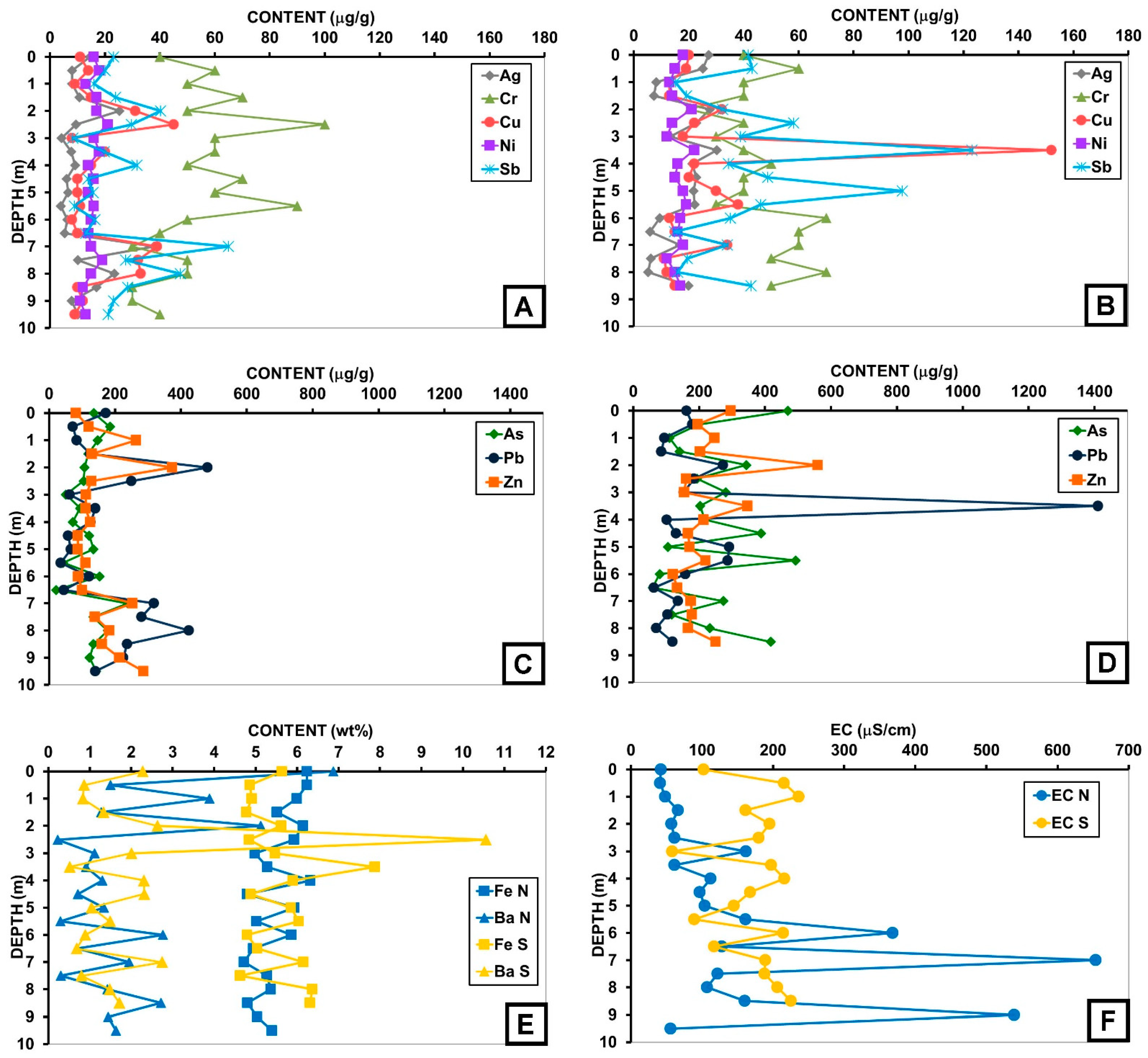[27] and explained as resulting from the joint treatment of two different mines from the same district. In the case of Pond S at San Carlos, the thinner, more enriched level (sample HB2-32) at 3.5 m depth (Figure 6) seems to be related to a higher sulfosalt content of that particular sample, due to the presence of some larger crystals in the sample.

With respect to the comparison between the two ponds, a slight generalised increase in the concentrations of almost all elements (except Fe₂O_{3 total} and S) is observed in the Pond S with respect to the Pond N. As mentioned above, these generalised increases in concentrations are usually related to a different origin of the minerals that were processed for the extraction of the ore. In fact, Pond S originates from the dumping of tailings from the last operating phase of the mine, between 1980 and 1996—that is, until the date of the mine’s definitive closure. In the latter period, old dumps from previous stages of mine operation were processed, which probably still contained significant quantities of Ag minerals that could not be effectively managed [20]. 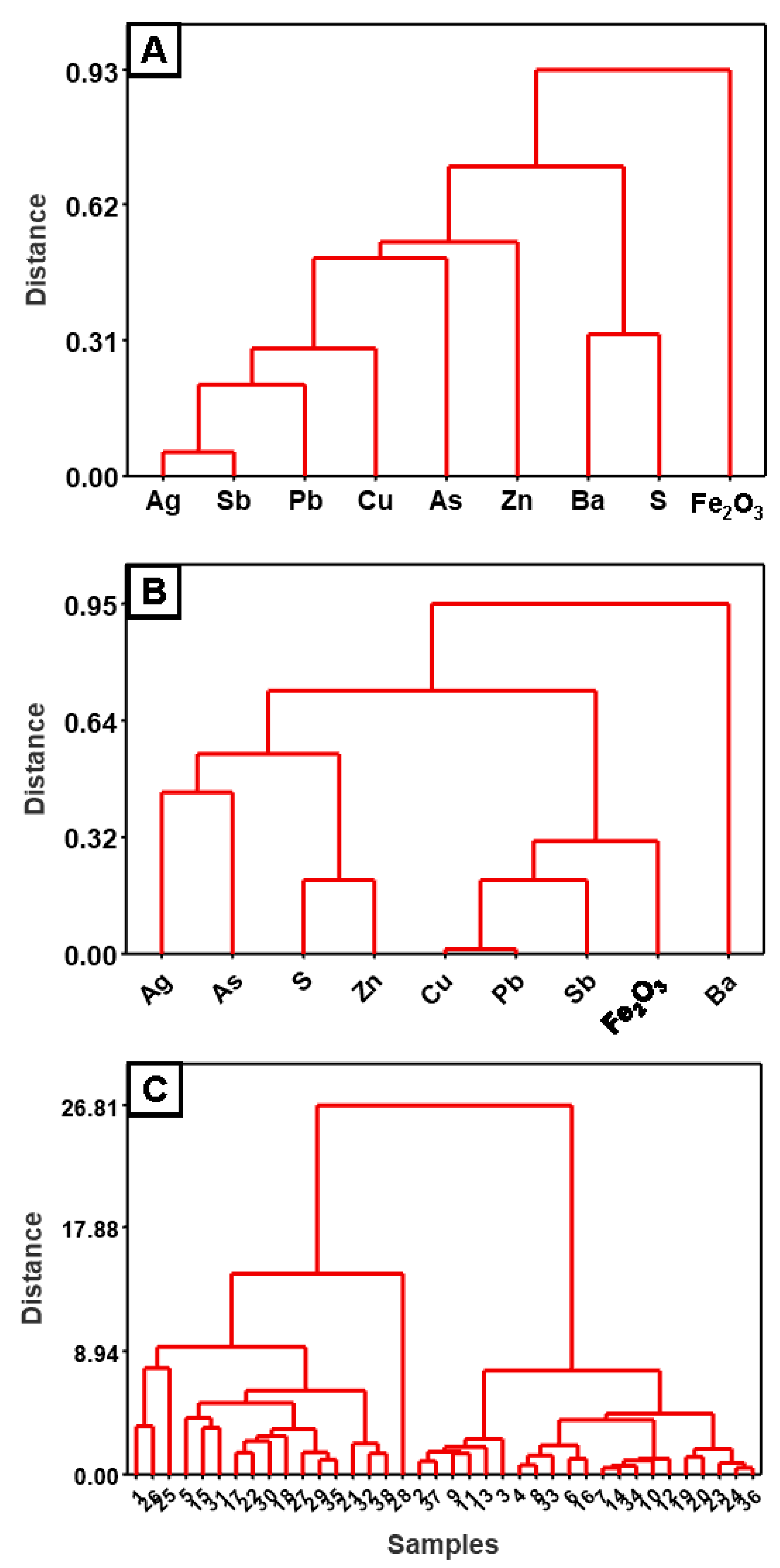To clarify this point, Figure 7 shows the cluster analysis of compositional variables from both ponds.

Figure 7A shows the cluster analyses of the variables (analysed elements) of Pond N. The paragenesis of the mineralisation is clearly reflected, with a significantly low distance between Ag, Sb, Pb, Cu, As and Zn, i.e., the main mineral elements of the mineralisation: argentiferous sulfosalts such as pyrargyrite (Ag₃SbS), freieslebenite (AgPbSbS₃), stephanite (AgSbS₄) and/or proustite (Ag₃AsS₃), galena (PbS), and stibnite (Sb₂S₃). 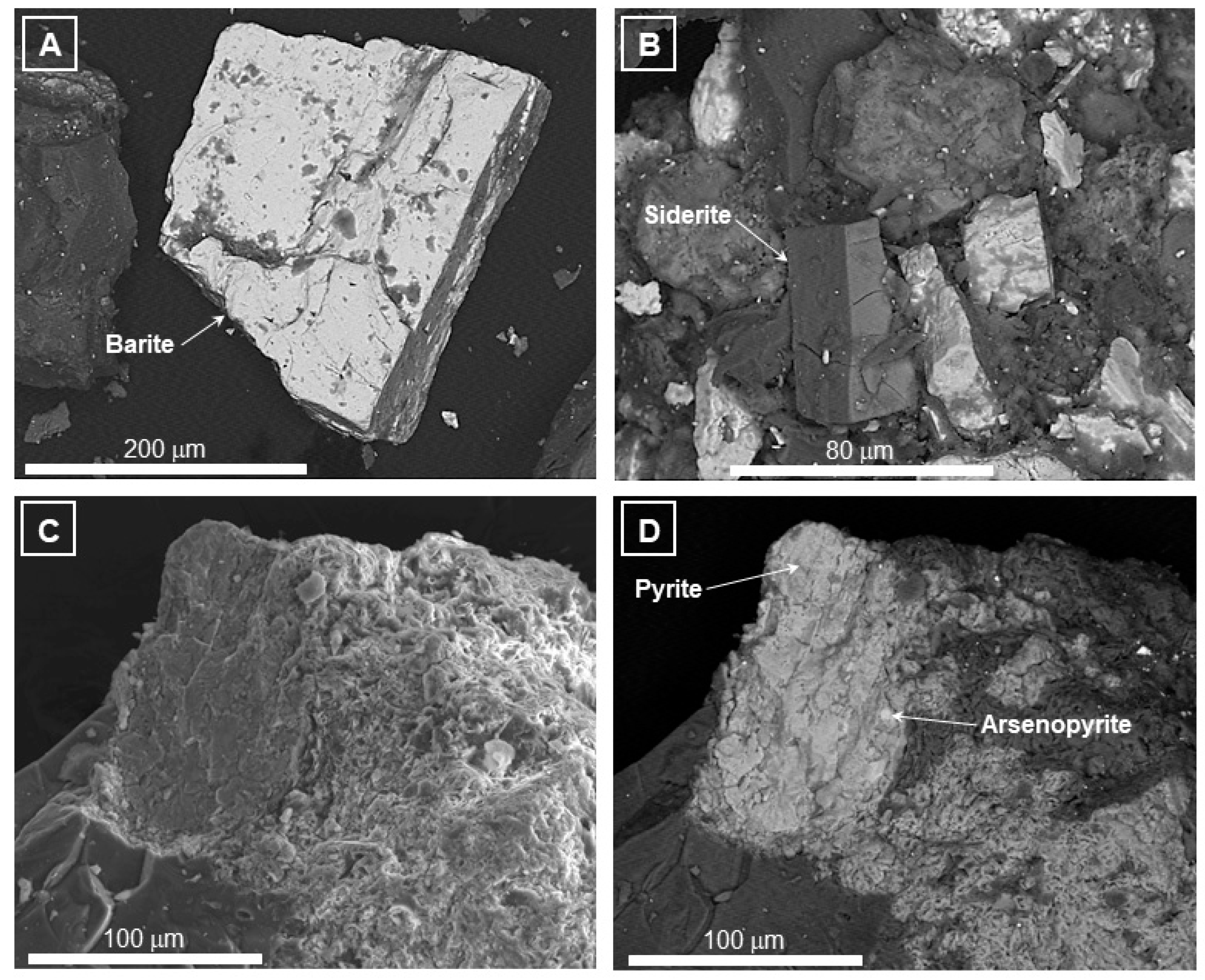Fe₂O_{3 total} is the furthest apart, probably because it is part of unmined gangue minerals such as siderite. S and Ba also have a low distance defined by the barite of the paragenesis. Figure 7B shows the cluster analysis results for elements in Pond S. In general, the behaviour resembles that of Pond N, although with slight differences. The fact that waste from the treatment of old dumps from at least two different mines, Santa Teresa and La Fuerza [20], was stored in pond S may have caused these differences. The greater distance of Ba in this pond could be explained by the fact that barite from the dumps was not processed. Figure 7C shows the two clusters of samples with close distances between them, the first cluster with samples mainly from Pond S (samples 21 to 38) and the second cluster with samples mainly from Pond N (samples 1 to 20). There is a greater distance between the two groupings, which indicates a different origin of the waste from one pond to the other. These results are very similar to those obtained by the authors in all mining districts analysed [33], reflecting the metallic signature of each mining district. The small differences always depend on the specific origin of the minerals to be treated and the metallurgical technology of the time in which they were accumulated: the mine, old dumps, etc. [20].

5.2. Mine Tailings Volumes from Aerial Imagery and LiDAR Data

The use of remote sensing techniques to measure surface elevation in time series has become widespread in recent years with the aim of estimating geomorphological changes and quantifying volumes of sediments and soils mobilized by wind, runoff, landslides or oceanic currents [9,34,35,36,37]. These studies are benefited from the development of increasingly precise equipment and sensors whose usefulness is continuously tested and verified [38,39]. Terrestrial laser scanning and ground photography are applicable to small areas, the latter being very useful at small scales and rugged terrains such as gullies, although their use may disturb the ground surface that is surveyed. The non-destructive alternative, and more suitable for larger areas, are sensors mounted on unmanned aerial vehicle (UAVs). Many studies combine the use of several techniques to integrate the advantages of each of them [35,40].

Those methods, however, cannot be applied directly to the case of anthropogenic landscape changes related to abandoned metal mining. Abandoned wastes have gained interest due to its environmental impact or the recovery of metals that were not extracted during mining stages [41,42]. Therefore, it is essential to quantify the volume of potentially toxic elements that pose a risk to ecosystem health or have an economic interest in the current strategies of circular economy. However, in these areas, high-resolution topography for the original landscape on which mining wastes were deposited may not be available. 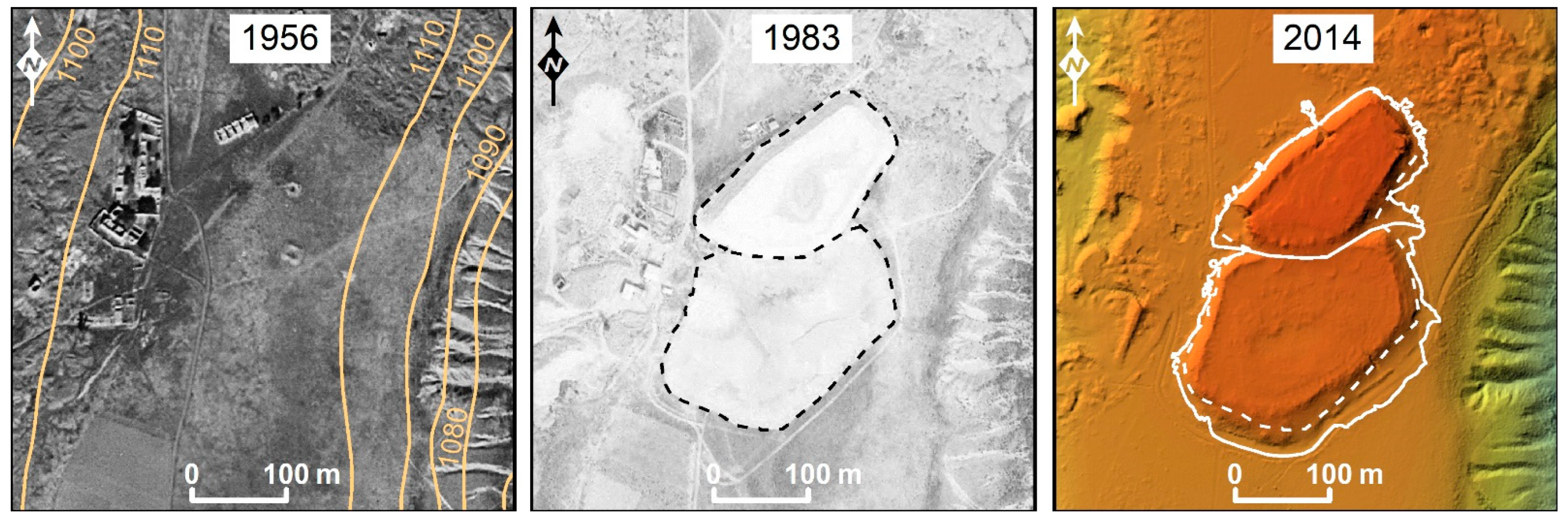Therefore, that surface is obtained by means of electrical tomography [18,33] or archival topographic maps and historical aerial photographs [7,17,43,44]. A geophysical procedure is only valid if there is a good contrast in the physical properties of wastes and basement and the fieldwork have a high economic and time cost. The digitisation of historical contour lines done in the Hiendelaencina area has several obvious advantages instead. It presents a greater precision in the calculation of the volumes by using aerial photographs for the topographical control of the base of the ponds. It is common that tailings ponds from mining operations at the beginning of the 20th century (Cartagena-La Unión and Mazarrón Districts, Spain) were established in stream valleys. In these cases, where the original topography of the pond base was not horizontal, having a topographical control is essential. Moreover, the results obtained in this way are highly accurate, and if sufficient mapping is available, the size and location of tailings deposits in mines abandoned many years ago can be tracked historically.

On the other hand, terrestrial laser scanning, ground photography or UAVs have a high resolution to capture topography, but they also have a high economic cost in equipment, data acquisition and data processing [38,39]. These disadvantages can be overcome with aerial imagery and LiDAR data that are publicly available, as in this work. Satellite LiDAR data are commonly used in large and inaccessible areas, and although it has lower accuracy than terrestrial or UAV sensors, it provides good preliminary estimations at the local scale [7,17,43,44]. Another issue of UAVs is that they require specific weather conditions and cannot fly over restricted zones. In the study presented here, the existence of an aerodrome 1 km NE of Hiendelaencina mine ponds prevents its use.

5.3. Environmental Problems and Legislation

One of the major problems of this type of waste lies in its medium-fine granulometry and the low cohesion of its particles, which causes significant erosion rates that favour the dispersion of its elements in the environment. There are several causes, both natural (wind and water erosion) and anthropic (movement of people, livestock, recreational activities and sporting activities) by which a mining slurry pond can disperse its constituents into the surrounding environment, being taken up by organisms living there [2]. One of the ways of assessing the potential ecological and anthropogenic impact is by means of the enrichment factor (EF). The EF is used to identify the anomalous concentration of hazardous metals in the environment [45]. To calculate it, a geochemical normalisation of the analysed metals against those of a conservative element (Fe) was performed. Then, it was evaluated using the following formula: EF = (M/Fe)_sample/(M/Fe)_blank, where (M/Fe)_sample is the ratio of the concentration of an element over the Fe concentration of the sample, and (M/Fe)_blank is the ratio of the concentration of a metal over the Fe concentration of the blank (sample BUS-1.5; Table 3). 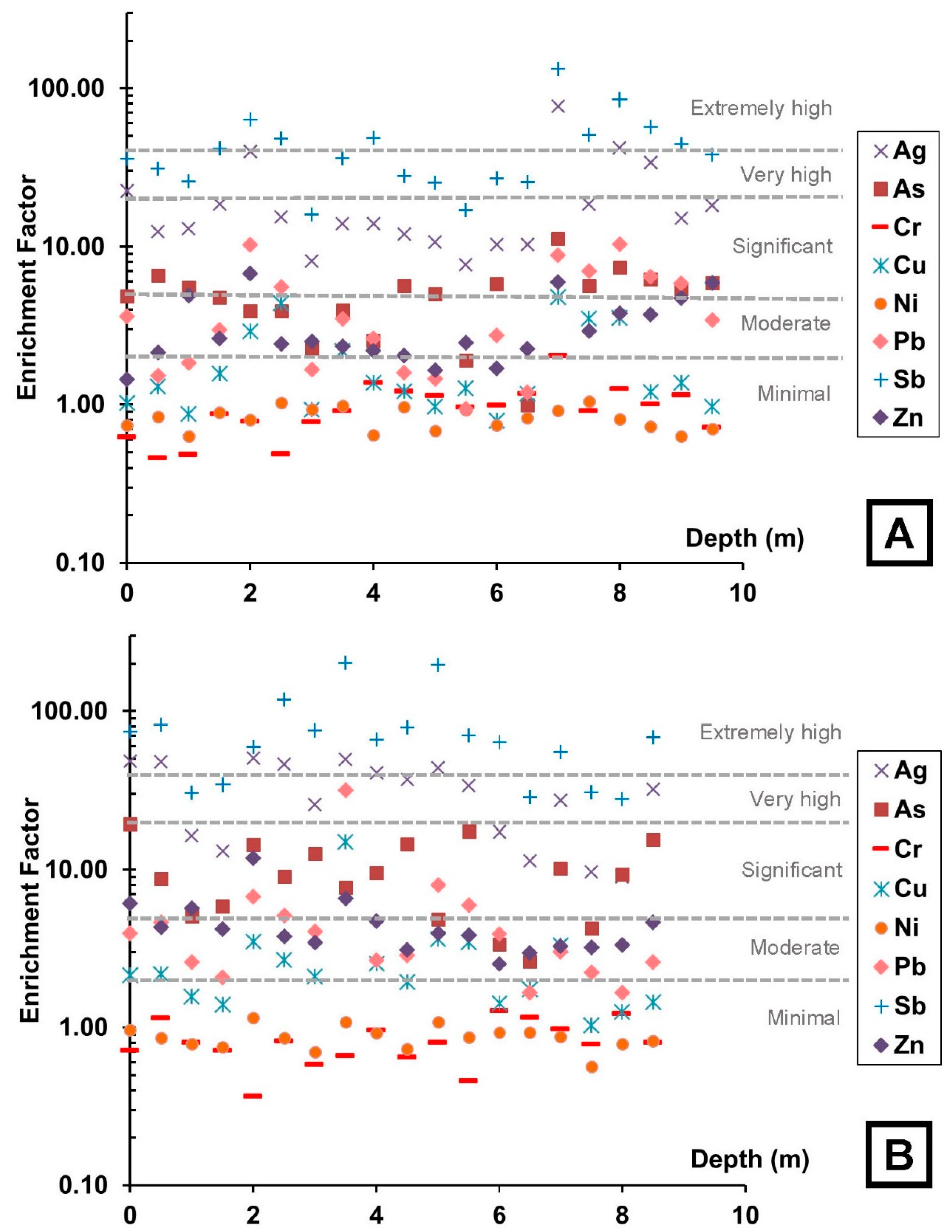According to Sutherland [45], there are five categories of contamination: minimal enrichment (EF < 2), moderate enrichment (2 < EF < 5), significant enrichment (5 < EF < 20), very high enrichment (20 < EF < 40) and extremely high enrichment (EF > 40).

The enrichment factors of the samples from both ponds are very similar to each other, and no changes in values with depth are observed (Figure 8). The slurries show high to extremely high EF in Ag and Sb, significant enrichment in As and moderate enrichment in Pb and Zn. The EF values for Cr, Cu and Ni are the lowest and correspond to the minimum enrichment category. These results are to be expected from the paragenesis of this mineralisation, which is mainly composed of Ag sulfosalts and sulphides of Pb, Zn, Fe and Cu. If these results are compared with the EF of other districts analysed ([28]; EF > 20), the latter show higher EF values than those of the Hiendelaencina ponds, reflecting the lower contaminant potential of this mining district. If the average metal contents in San Carlos are also compared with those published for similar slurries from other abandoned mining districts [27,29,33,46], the concentration of potentially hazardous elements such as As, Cu, Pb, Sb or Zn in other districts is significantly higher.

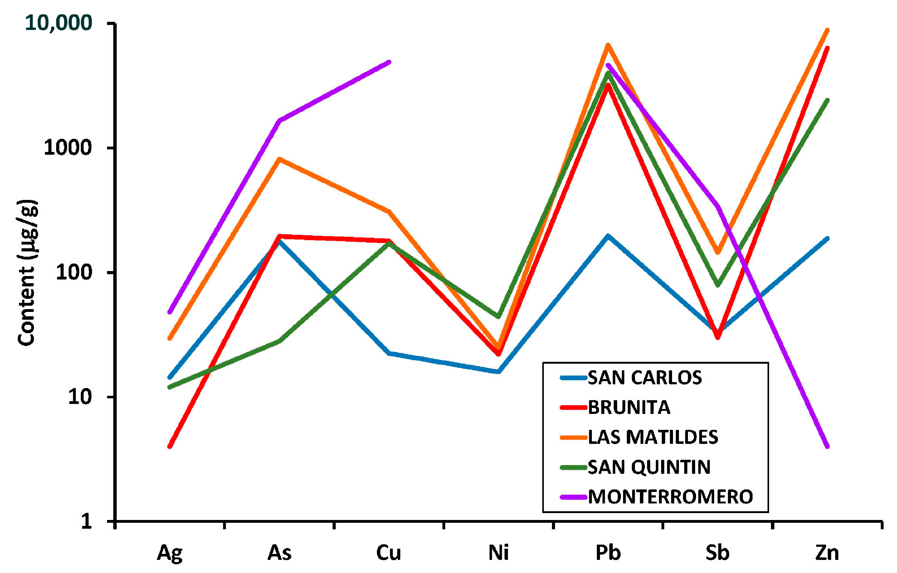
Figure 9 shows the average values for San Carlos together with the average values for ponds in three important mining districts in Spain: Brunita and Las Matildes (Cartagena La Unión District), San Quintín (Valle de Alcudia District) and Monterromero (Riotinto District). It can be clearly seen that the levels of potentially hazardous elements in the San Carlos Pond (Hiendelaencina) are significantly lower than those measured in the ponds of the other three mining districts studied. This may be due to the fact that the San Carlos slurries come from more modern metallurgical tailings processes, with more efficient metallurgical technologies, which optimised the utilisation of the metals present in the tailings dumps [20]. In some of the ponds in the other districts, the measured values could make them exploitable, depending on the world price of the substance. Furthermore, the samples from the Brunita, Las Matildes and Monterromero Ponds have an acidic pH, while the San Carlos samples have an alkaline pH, which means a lower capacity for the mobilisation of potentially hazardous substances in the case of Hiendelaencina Pond. All these data reflect the lower pollution potential of this district compared to the rest of the mining districts studied.

Generally, the parameter that usually determines the higher or lower degree of mobility of metals in the environment is the pH. Although no direct relationship between the physicochemical parameters and the composition of the pond was observed at first sight, it is known that sulphides with a metal/sulphide ratio = 1 (e.g., sphalerite, galena or chalcopyrite) do not normally produce acidity when the oxidising agent is oxygen [47]. Therefore, slurries from this type of mineralisation usually have alkaline characteristics. Even so, considering the significant percentage in weight of siderite estimated by XRD (Table 1), it is important to study the pH of the slurry, as sulphides can generate acidity upon weathering [2]. With regard to the Spanish applicable legislation on slurry pond contamination, it is necessary to consult Royal Decree 1310/1990, which establishes the limit concentrations of potentially dangerous elements that soils may contain depending on the pH (

Table 6. Concentration limit values for potentially toxic elements in soils according to Royal Decree 1310/1990 [48], based on EEC directives over reuse of contaminated soils.

Elements	Limit Values in Soils with pH > 7 (μg/g)
Cd	3
Cr	150
Cu	210
Ni	112
Pb	300
Zn	450

).

The pH values of all slurry samples are >7; therefore, Pb is the only metal exceeding the permitted values in 4 of the 38 samples analysed. The contents of the other elements do not exceed the permitted values. Apart from the metal contents envisaged by the present legislation, two other elements (As and Sb) are present in significant amounts in the mine ponds and could pose a risk for the environment. Moreover, As and Sb are metalloids whose degree of mobilisation increases with the pH, as is the case for the study area, where alkaline pH values have been measured. However, the pseudo-total As concentrations are not a good indicators of mobilisation and the potential environmental impact, because As fractions (As(III) and As(V)) differ in their solubility, particularly under different environmental conditions, e.g., [49]. In order to properly discriminate the degree of arsenic mobilisation and potential risk of transfer to aqueous systems, fractionation studies and leaching tests should be used. Similar conclusions can be obtained for Sb, as their degree of mobilisation also depends on the different Sb fraction (Sb(III) and Sb(V)) concentrations. This is beyond the scope of this work and, consequently, has not been considered here, but they would be envisaged for future works in the area. However, it is worthy to say that a recent work about the physicochemical properties of both surface and groundwater discharge points around the mine ponds [50] has revealed very low (<1 µg/L) concentration values of the total As and Sb, independently of the climate conditions (different field sampling campaigns were carried out to evaluate potential differences between the wet and dry periods during the year). The results obtained by the authors seem to confirm that, despite the high concentration values of the metalloids found in the pond samples, its degree of mobilisation towards the aqueous systems is very reduced. This seems to exclude the polluting potential of these ponds in relation to the surrounding aqueous systems, but its dispersion from mobilisation agents different from water cannot be completely ruled out. As stated in [7], the entire pond perimeter is exposed to the combined effects of water, wind, gravity and anthropogenic actions. Consequently, measures to restore and/or stabilise the ponds should be undertaken to reduce the high rate of erosion and the dispersion of potentially toxic metals.

In summary, although the minor polluting potential of these ponds is evident, the quantities are significant enough to require a detailed geo-environmental study and the implementation of appropriate management to minimise the risk both for the environment and for the native population and visitors.

6. Conclusions

The combined application of geochemical, mineralogical and LiDAR techniques has enabled the successful estimation of the tonnages of pollutants in two abandoned mine tailings ponds. The mineralogical composition of the slurry ponds at the San Carlos mine is quite homogeneous, consisting mainly of quartz, muscovite, potassium feldspar, siderite and barite, with very little presence of metallic minerals from the paragenesis. Regarding chemical composition, there has been observed significant, but not particularly high, contents of As, Cr, Pb, Sb and Zn, which are potentially hazardous elements from the ore. No internal compositional zonation of the ponds has been detected, although higher amounts of Ag, As, Cu, Pb, Sb and Zn have been measured in Pond S than in Pond N. This could be due to the different mineralisation content of the reworked dumps from at least two different mines. The low content of Fe and S, the presence of siderite and the alkaline pH values confirm the absence of acidic drainage from the slurry ponds. The slurries show extremely high EF values for Ag and Sb, significant ones for As and moderate values for Pb and Zn. These values are high, although lower than in other similar mining districts. The combined use of aerial imagery, topographic mapping, LiDAR data and the mineralogical and chemical composition of the ponds has allowed calculating the contents of potentially hazardous elements stored in the ponds. Of the 745 tonnes that are susceptible to dispersion into the environment, 198 tonnes of As, 213 tonnes of Pb and 203 tonnes of Zn stand out. In view of the results obtained in this study, a complete characterisation of the area (mine and surrounding soils, surface water, surrounding cultivated areas, etc.) is necessary, as well as an adequate management to minimise the negative effects on the environment, the population and visitors to Hiendelaencina.

References

1. Leblanc, M.; Morales, J.A.; Borreho, J.; Elbaz-Poulichet, F. 4,500-Year-old mining pollution in southwestern Spain: Long-term implications for modern mining pollution. Econ. Geol. 2000, 95, 655–662. [Google Scholar] [CrossRef]
2. González, O. Impacto Ambiental de las Áreas de Minería Metálica: Aplicación de Metodologías Analíticas no Destructivas al Análisis Geoquímico. Doctoral Thesis, Universidad Autónoma de Barcelona, Barcelona, Spain, 2011; p. 388. [Google Scholar]
3. Baker, E.; Davies, M.; Fourie, A.; Mudd, G.; Thygesen, K. Chapter II. Mine Tailings Facilities: Overview and Industry Trends. In Towards Zero Harm: A Compendium of Papers Prepared for the Global Tailings Review; Oberle, B., Brereton, D., Mihaylova, A., Eds.; Global Tailings Review: London, UK, 2020; pp. 14–25. [Google Scholar]
4. Lindsay, M.B.J.; Moncur, M.C.; Bain, J.G.; Jambor, J.L.; Ptacek, C.J.; Blowes, D.W. Geochemical and mineralogical aspects of sulfide mine tailings. Appl. Geochem. 2015, 57, 157–177. [Google Scholar] [CrossRef]
5. López Gómez, A. El distrito minero de Hiendelaencina (Guadalajara). Cuad. Geogr. 1969, 6, 211–250. [Google Scholar]
6. Martínez Frías, J. The Hiendelaencina mining district (Guadalajara, Spain). Miner. Depos. 1992, 27, 206–212. [Google Scholar] [CrossRef]
7. Martín-Velázquez, S.; Rodríguez-Santalla, I.; Ropero-Szymañska, N.; Gómez-Ortiz, D.; Martín-Crespo, T.; De Ignacio, C. Geomorphological Mapping and Erosion of Abandoned Tailings in the Hiendelaencina Mining District (Spain) from Aerial Imagery and LiDAR Data. Remote Sens. 2022, 14, 4617. [Google Scholar] [CrossRef]
8. Pérez, A.M.; Gracia, F.J.; Vallejo, I.; Barrera, J.A.; Ojeda, J. Estudio Morfométrico y Volumétrico del Retroceso de Acantilados Mediante Escáner Láser Terrestre y Modelado 3d. Aplicación al Acantilado de Torre Bermeja (Cádiz); Actas de las VI Jornadas de Geomorfología Litoral; Universidad Rey Juan Carlos and Ministerio deCiencia e Innovación: Tarragona, Spain, 2011. [Google Scholar]
9. Rodríguez-Santalla, I.; Gomez-Ortiz, D.; Martín-Crespo, T.; Sánchez-García, M.J.; Montoya-Montes, I.; Martín-Velázquez, S.; Barrio, F.; Serra, J.; Ramírez-Cuesta, J.M.; Gracia, F.J. Study and Evolution of the Dune Field of La Banya Spit in Ebro Delta (Spain) Using LiDAR Data and GPR. Remote Sens. 2021, 13, 802. [Google Scholar] [CrossRef]
10. Rodríguez-Santalla, I.; Díez-Martínez, A.; Navarro, N. Vulnerability Analysis of the Riumar Dune Field in El Garxal Coastal Wetland (Ebro Delta, Spain). J. Mar. Sci. Eng. 2021, 9, 601. [Google Scholar] [CrossRef]
11. Fernández-Lozano, J.; Gutiérrez-Alonso, G.; Fernández-Morán, M. Using airborne LiDAR sensing technology and aerial orthoimages to unravel Roman water supply systems and gold works in NW Spain (Eria valley, León). J. Archaeol. Sci. 2015, 53, 356–373. [Google Scholar] [CrossRef]
12. Andrés-Bercianos, R.; Fernandez-Lozano, J.; Alonso-Gavilán, G. Documentación de explotaciones mineras romanas y caracterización geológica de los placeres auríferos del piedemonte de Justel (Zamora). In The Archaeology of ‘Underdog Sites’ in the Douro Valley: From Prehistory to the Modern Age; Sánchez de la Parra-Pérez, S., Díaz-Navarro, S., Fernández-Lozano, J., Jiménez Gadea, J., Eds.; Archaeopress Publishing Ltd.: Oxford, UK, 2021; pp. 329–344. ISBN 978-1-78969-989-0. [Google Scholar]
13. Matías, R.; Llamas, B. Analysis Using LIDAR and Photointerpretation of Las Murias-Los Tallares (Castrocontrigo, León-Spain): One of the Biggest Roman Gold Mines to Use the “Peines” System. Geoheritage 2019, 11, 381–397. [Google Scholar] [CrossRef]
14. Fernández Lozano, J.; Gutiérrez Alonso, G. Aplicación de LiDAR aerotransportado para la cartografía de antiguas labores mineras romanas en el noroeste peninsular. Mapping 2014, 23, 22–29. [Google Scholar]
15. Slob, S.; Hack, R. 3D Terrestrial Laser Scanning as a New Field Measurement and Monitoring Technique. In Engineering Geology for Infrastructure Planning in Europe; Hack, R., Azzam, R., Charlier, R., Eds.; Lecture Notes in Earth Sciences; Springer: Berlin, Germany, 2004; Volume 104, pp. 179–189. ISBN 978-3-540-21075-7. [Google Scholar]
16. Howle, J.F.; Alpers, C.N.; Bawden, G.W.; Bond, S. Quantifying the Eroded Volume of Mercury-Contaminated Sediment Using Terrestrial Laser Scanning at Stocking Flat, Deer Creek, Nevada County, California, 2010–2013; Scientific Investigations Report 2015–5179; United States Geological Survey: City of Fairfax, VA, USA, 2013. [Google Scholar]
17. Witt, E.C. Use of lidar point cloud data to support estimation of residual trace metals stored in mine chat piles in the Old Lead Belt of southeastern, Missouri. AIMS Environ. Sci. 2016, 3, 509–524. [Google Scholar]
18. Martínez-Segura, M.; Vásconez-Maza, M.; García-Nieto, M.C. Volumetric characterisation of waste deposits generated during the production of fertiliser derived from phosphoric rock by using LiDAR and electrical resistivity tomography. Sci. Total Environ. 2020, 716, 137076. [Google Scholar] [CrossRef]
19. Instituto Geográfico Nacional (IGN). Centro Nacional de Información Geográfica. Available online: https://www.cnig.es (accessed on 24 May 2021).
20. Gismera Angona, A. Hiendelaencina y sus Minas de Plata; Aache Editorial: Guadalajara, Spain, 2018; p. 432. [Google Scholar]
21. Calvo, M.; Sevillano, E. Famous Mineral Localities: Hiendelaencina, Spain. Mineral. Rec. 1992, 23, 241–249. [Google Scholar]
22. Portero, J.M.; Pérez González, A.; Díaz Molina, M.; Gallardo, M.J.; González Lodeiro, F.; Aguilar, M.J.; Leal, C. Mapa Geológico Nacional Serie MAGNA escala 1:50.000. Hoja 460 (Hiendelaencina); Instituto Geológico y Minero de España: Madrid, Spain, 1990. [Google Scholar]
23. García, G. Minas de Plata de Hiendelaencina (Fundición y Lavadero San Carlos). MTI Minas Castilla-La Mancha, Mineralogía Topográfica Ibérica 1995. Available online: https://mti-minas-castillalamancha.blogspot.com/ (accessed on 3 March 2022).
24. Instituto Geológico y Minero de España (IGME). Información Sobre la Balsa 0460-3-0001. Available online: http://info.igme.es/balsas/InfoBalsa.aspx?id=0460-3-0001 (accessed on 25 May 2021).
25. Hubbard, C.R.; Snyder, R.L. RIR—Measurement and Use in Quantitative XRD. Powder Diffr. 1988, 3, 74–77. [Google Scholar] [CrossRef] [Green Version]
26. Instituto Geográfico Nacional (IGN). Mapa Topográfico del Municipio de Hiendelaencina 1:25,000; Instituto Geográfico Nacional: Madrid, Spain, 1954. [Google Scholar]
27. Martín-Crespo, T.; Gómez-Ortiz, D.; Martín-Velázquez, S.; Martínez-Pagán, P.; De Ignacio, C.; Lillo, J.; Faz, Á. Geoenvironmental characterization of unstable abandoned mine tailings combining geophysical and geochemical methods (Cartagena-La Union district, Spain). Eng. Geol. 2018, 232, 135–146. [Google Scholar] [CrossRef]
28. Martín-Crespo, T.; Gómez-Ortiz, D.; Martínez-Pagán, P.; De Ignacio-San José, C.; Martín-Velázquez, S.; Lillo, J.; Faz, A. Geoenvironmental characterization of riverbeds affected by mine tailings in the Mazarrón district (Spain). J. Geochem. Explor. 2012, 119–120, 6–16. [Google Scholar] [CrossRef]
29. Martín-Crespo, T.; Gómez-Ortiz, D.; Martín-Velázquez, S.; Esbrí, J.M.; de Ignacio-San José, C.; Sánchez-García, M.J.; Montoya-Montes, I.; Martín-González, F. Abandoned mine tailings in cultural itineraries: Don Quixote Route (Spain). Eng. Geol. 2015, 197, 82–93. [Google Scholar] [CrossRef]
30. Mansson, E. Investigation of Particle Sizes, Beach Profiles and Compounds in Tailings Dams. Master’s Thesis, Lund University, Lund, Sweden, 2014. [Google Scholar]
31. Quille, M.E.; O’Kelly, B.C. Geotechnical properties of zinc/lead mine tailings from Tara Mines, Ireland. In Proceedings of the ASCE GeoShanghai, Shanghai, China, 3–5 June 2010; Volume 204, pp. 111–117. [Google Scholar]
32. Mhlongo, S.E.; Makatu, F.L.; Malaza, N.K.; Ramalata, A.T. Evaluation of copper tailings from the abandoned Messina Mine for possible reuse in recreational projects, South Africa. J. Degrad. Min. Lands Manag. 2022, 9, 3359–3366. [Google Scholar] [CrossRef]
33. Martín-Crespo, T.; Martín-Velázquez, S.; Gómez-Ortiz, D.; De Ignacio-San José, C.; Lillo-Ramos, J. A geochemical and geophysical characterization of sulfide mine ponds at the Iberian Pyrite Belt (Spain). Water Air Soil Pollut. 2011, 217, 387–405. [Google Scholar] [CrossRef] [Green Version]
34. Gómez-Gutiérrez, A.; Schnabel, S.; Berenguer-Sempere, F.; Lavado-Contador, F.; Rubio-Delgado, J. Using 3D photo-reconstruction methods to estimate gully headcut erosion. Catena 2014, 120, 91–101. [Google Scholar] [CrossRef]
35. Stumpf, A.; Malet, J.-P.; Allemand, P.; Deseilligny, M.P.; Skupinski, G. Ground-based multi-view photogrammetry for the monitoring of landslide deformation and erosion. Geomorphology 2015, 231, 130–145. [Google Scholar] [CrossRef]
36. Pineux, N.; Lisein, J.; Swerts, G.; Bielders, C.; Lejeune, P.; Colinet, G.; Degré, A. Can DEM time series produced by UAV be used to quantify diffuse erosion in an agricultural watershed? Geomorphology 2017, 280, 122–136. [Google Scholar] [CrossRef]
37. Kariminejad, N.; Hosseinalizadeh, M.; Pourghasemi, H.R.; Tiefenbacher, J.P. Change detection in piping, gully head forms, and mechanisms. Catena 2021, 206, 105550. [Google Scholar] [CrossRef]
38. Castillo, C.; Perez, R.; James, M.R.; Quinton, J.N.; Taguas, E.V.; Gómez, J.A. Comparing the accuracy of several field methods for measuring gully erosion. Soil Sci. Soc. Am. J. 2012, 76, 1319–1332. [Google Scholar] [CrossRef] [Green Version]
39. Glendell, M.; Mcshane, G.; Farrow, L.; James, M.; Quinton, J.; Anderson, K.; Evans, M.; Benaud, P.; Rawlins, B.; Morgan, D.; et al. Testing the utility of structure from motion photogrammetry reconstructions using small unmanned aerial vehicles and ground photography to estimate the extent of upland soil erosion. Earth Surf. Process Landf. 2017, 42, 1860–1871. [Google Scholar] [CrossRef] [Green Version]
40. Stöcker, C.; Eltner, A.; Karrasch, P. Measuring gullies by synergetic application of UAV and close range photogrammetry—A case study from Andalusia, Spain. Catena 2015, 132, 1–11. [Google Scholar] [CrossRef]
41. Tarolli, P.; Giulia, S. Human topographic signatures and derived geomorphic processes across landscapes. Geomorphology 2016, 255, 140–161. [Google Scholar] [CrossRef] [Green Version]
42. Kinnunen, P.; Karhu, M.; Yli-Rantala, E.; Kivikytö-Reponen, P.; Mäkinen, J. A review of circular economy strategies for mine tailings. Chem. Eng. Technol. 2022, 8, 100499. [Google Scholar] [CrossRef]
43. Martín Duque, J.F.; Zapico, I.; Oyarzun, R.; López García, J.A.; Cubas, P. A descriptive and quantitative approach regarding erosion and development of landforms on abandoned mine tailings: New insights and environmental implications from SE Spain. Geomorphology 2015, 239, 1–16. [Google Scholar] [CrossRef] [Green Version]
44. Trybała, P.; Kaczan, W.; Górecki, A. Mining Waste Volume Estimation Using Airborne Lidar Data and Historical Maps: A Case Study of Tailing Piles in Szklary, Lower Silesia. Environ. Sci. Proc. 2021, 9, 32. [Google Scholar]
45. Sutherland, R.A. Bed sediment-associated trace metals in an urban stream, Oahu, Hawaii. Environ. Geol. 2000, 39, 611–626. [Google Scholar] [CrossRef]
46. Martín-Crespo, T.; Gómez-Ortiz, D.; Martín-Velázquez, S.; Martínez-Pagán, P.; De Ignacio, C.; Lillo, J.; Faz, Á. Abandoned mine tailings affecting riverbed sediments in the Cartagena–La Union District, Mediterranean Coastal Area (Spain). Remote Sens. 2020, 12, 2042. [Google Scholar] [CrossRef]
47. Nordstrom, D.K.; Alpers, C.N. Geochemistry of acid mine waters. In The Environmental Geochemistry of Mineral Deposits, Processes, Techniques, and Health Issues; Plumlee, G.S., Logsdon, M.J., Filipek, L.F., Eds.; Reviews in Economic Geology; Society of Economic Geologists: Littleton, CO, USA, 1999; Volume 6A, pp. 133–160. ISBN 9781629490137. [Google Scholar]
48. Boletín Oficial del Estado (BOE). Real Decreto 1310/1990, de 29 de Octubre, que Regula la Utilización de los Lodos de Depuración en el Sector Agrario; Agencia Estatal Boletín Oficial del Estado (AEBOE): Madrid, Spain, 1990; Volume 262. [Google Scholar]
49. Martiñá-Prieto, D.; Cancelo-González, J.; Barral, M.T. Arsenic mobility in As-containing soils from geogenic origin: Fractionation and leachability. J. Chem. 2018, 2018, 7328203. [Google Scholar] [CrossRef] [Green Version]
50. Pryimak, V. Hidroquímica de las Aguas de los Pozos Mineros de Hiendelaencina. Evaluación de Posibles Flujos Contaminantes Desde las Balsas de Lodos Mediante Tomografía Eléctrica. Master’s Thesis, Universidad de Alcalá de Henares-Universidad Rey Juan Carlos, Madrid, Spain, 2022. [Google Scholar]
Figure 1. Situation of the mining district of Hiendelaencina. The San Carlos Mine tailings and the sampling points of Pond N and Pond S are shown. Coordinates are in kilometres.
Remotesensing 15 01423 g001
Figure 2. Treatment and disposal facilities at the San Carlos Mine in 1995. (A) Crushing plant; (B) Flotation cells; (C) Discharge system; (D) View of the slurry pond [23].
Remotesensing 15 01423 g002
Figure 3. Sampling of Pond N (A) and Pond S (B).
Remotesensing 15 01423 g003
Figure 4. Cartographic documents used in the calculation of tailings (from left to right): 1956 aerial image, 1983 aerial image and 2014 digital terrain model. The continuous lines on the 1956 aerial image are the contour intervals of the 1954 topographic map (altitude values in metres). The dashed lines above the 1983 aerial image and the 2014 DTM show the mine pond boundaries during the time they were operational. The solid lines in the 2014 DTM indicate the tailing boundaries mapped in the 2015 aerial image.
Remotesensing 15 01423 g004
Figure 5. High-resolution SEM images of the identified minerals. (A) Barite (backscattered electron image); (B) siderite (backscattered electron image); (C) pyrite (secondary electron image); (D) pyrite and arsenopyrite (backscattered electron image).
Remotesensing 15 01423 g005
Figure 6. In-depth distribution profiles: (A) Ag, Cr, Cu, Ni and Sb from Pond N; (B) Ag, Cr, Cu, Ni and Sb from Pond S; (C) As, Pb and Zn from Pond N; (D) As, Pb and Zn from Pond S; and (E,F) Fe and Ba and electrical conductivity from both ponds (N = north; S = south).
Remotesensing 15 01423 g006
Figure 7. Cluster analysis of the elements in Pond N (A) and in Pond S (B); (C) cluster analysis of the total of samples from both ponds: samples 1 to 20 belong to Pond N, and samples 21 to 38 belong to Pond S.
Remotesensing 15 01423 g007
Figure 8. Enrichment factor (EF) of slurry samples from Hiendelaencina: (A) Pond N; (B) Pond S.
Remotesensing 15 01423 g008
Figure 9. Comparison of the mean concentrations of potentially toxic elements in the ponds of San Carlos (present study), Brunita [27], Las Matildes [47], San Quintín [29] and Monterromero [33].
Remotesensing 15 01423 g009