Identification and Analysis of Unstable Slope and Seasonal Frozen Soil Area along the Litang Section of the Sichuan–Tibet Railway, China

Abstract

The Sichuan–Tibet Railway (STR) is currently under construction and serves as an important transportation route in western China. Identifying potential geohazards along the route is important for project construction. However, research on the frozen soil of the Western Sichuan Plateau, and on frozen soil identification using interferometric synthetic aperture radar (InSAR) is relatively negligible. As a low-cost, all-weather spatial geodesy tool, InSAR is frequently used for geohazard identification. We selected a study area located along the Litang section of the STR, starting from Litang County in the east and extending 60 km to the west. The geological conditions along the line are complex, with numerous fault zones and hidden danger points for landslide. To identify unstable slopes along the line, distribute scatterer InSAR (DS-InSAR) was used to obtain surface displacement information from 2018 to 2021. Based on the displacement information obtained from the ascending and descending orbit images from Sentinel-1, a spatial density clustering method identified 377 and 388 unstable slopes in the study area, respectively, of these, 132 were consistent. The identified unstable slopes were mostly located in areas with a relatively high altitude and moderate slope. The Luanshibao landslide, which is a typical landslide in the study area, had notable signs of displacement, where the displacement rate along the back edge of the landslide can reach 20 mm/a. An inversion method for the seasonal frozen soil area distribution was proposed based on the periodic subsidence and uplift model and time-series monitoring data; the calculated seasonal freeze–thaw amplitude exceeded 20 mm. Further analysis revealed a 2-month lag in the response of the freeze–thaw phenomenon to the air temperature. This study demonstrated that DS-InSAR offers optimal surface displacement data, which can provide an important basis to identify engineering geological hazards.

1. Introduction

Landslides are a disaster phenomenon in which the geotechnical body on a slope slides downward along the damaged penetrating surface, as well as slopes characterized by an unstable state that may evolve into a landslide disaster [1]. The route of the Sichuan–Tibet Railway (STR) is mostly located in mountain and valley areas, with complex geological structures and strong neotectonic movement. A series of unstable slopes and high-altitude frozen soil areas are formed under the coupling effect of internal and external dynamics [2,3]. Diverse types of geological hazards have increased the difficulty of STR construction and operation [4,5]. Therefore, identifying the unstable slopes and seasonal frozen soil in this region is of great significance, as well as investigating the development patterns associated with unstable slopes and seasonal frozen soil. This will ensure the safety of major engineering constructions, human life, and property in this region.

With recent rapid progress in science and technology, especially the emergence of remote sensing, wireless communication, and various sensing technologies, the identification, monitoring, and early warning of geological hazards have become important tools for their prevention and control [6]. Interferometric synthetic aperture radar (InSAR) is advantageous owing to its all-weather and all-day operation, wide coverage, high spatial resolution, non-contact, and low comprehensive costs [7,8]. InSAR provides continuous tracking and observation of small ground deformation areas across a wide scale, such that it has the unique ability to identify and continuously observe deformation areas [9,10]. For instance, Shi et al. [11] used small baseline subset InSAR (SBAS-InSAR) to identify and analyze geological hazards, such as unstable slopes, in the Litang to Batang region. Zhang et al. [12] used InSAR to identify potential landslides in the Danba region of Sichuan Province and analyzed the deformation characteristics of typical landslides. Zhang et al. [13] used the stacking-InSAR technique to identify 72 potential landslides in the western Sichuan region.

Similarly, InSAR has been widely used for seasonal frozen soil displacement monitoring. For example, Liu et al. [14] used InSAR to obtain displacement information for the north slope of a frozen soil area in Alaska; their results showed that 1–4 cm of subsidence occurred in the area due to the melting of subsurface ice at the upper limit of frozen soil from 1992–2000. Jia et al. [15] inferred the active layer thickness in the Qinghai–Tibet Plateau based on InSAR results combined with a simplified deformation-active layer thickness relationship model. Most studies on frozen soil areas in China have focused on the Qinghai–Tibet Plateau and northeastern China, while relatively negligible research has been conducted on the frozen soil of the Western Sichuan Plateau and even fewer studies on frozen soil identification using InSAR [16,17]. The ground surface decreases in strength under the action of freeze–thaw cycle, which is the main factor affecting the construction and operation of STR. The snow melt infiltration increases the water content of the surface soil, and the strength of the soil is further reduced because of freezing and thawing. The vertical displacement of the surface is likely to exceed the allowable value of roadbed. Identification and inversion of vertical displacement changes in seasonal frozen soil areas along the STR can provide valuable information for construction and operation. The seasonal frozen soil identification method used in this study is based on various frozen soil displacement curves, without the need for factors such as temperature and soil type or physical and empirical models of frozen soil, thus reducing the computational load and complexity of identification. This identification method can be regarded as an unsupervised classification method, where the final results are a true reflection of the displacement patterns of frozen soil [18].

Time-series InSAR has developed rapidly since Ferretti et al. (2001) proposed persistent scatterer InSAR (PS-InSAR). Berardino et al. (2002) proposed the SBAS-InSAR, which can partially suppress the effect of temporal decorrelation, but the accuracy of deformation monitoring is low [19]. Ferretti (2011) proposed the second-generation permanent scatterer technique (SqueeSAR) [20]. Since then, research hotspots in the field of time-series InSAR have gradually shifted to the analysis of distributed targets. Unlike the physical properties of PS targets, DS refers to point targets where backscatter dominates without any scatterers in the radar resolution cell. By combining PS and DS points for analysis, the DS-InSAR method significantly improves the distribution density of monitoring points and has been increasingly applied to the monitoring of unstable slopes and roads. The accuracy of the DS-InSAR method is slightly lower than that of the PS-InSAR method, but the extracted point density is greatly improved, which is helpful to obtain more detailed surface displacement information.

The Litang section of STR is the subject area of this study. This area is one of the two typical seasonal frozen soil distribution areas along the STR, the other being Xinduqiao. In addition, Litang is a high-altitude area along the STR. The terrain in the study area is dominated by mountains and basins, surface vegetation cover is sparse, and there are mostly distributed scatterers on the SAR images. Therefore, we first carried out a terrain visibility evaluation of the study area and then used DS-InSAR to process the ascending and descending Sentinel data to obtain displacement results from January 2018 to February 2021. A spatial density clustering algorithm and DEM were used to identify the locations of unstable slopes, followed by a discussion of the factors affecting their distribution, such as elevation, slope, and faults. The time-series displacement data were analyzed in combination with the periodic subsidence and uplift model to obtain seasonal frozen soil distribution results in the study area. This study can provide data support for the construction and operation of STR, and expand the application of InSAR in the study of seasonal frozen soil.

2. Materials and Methods

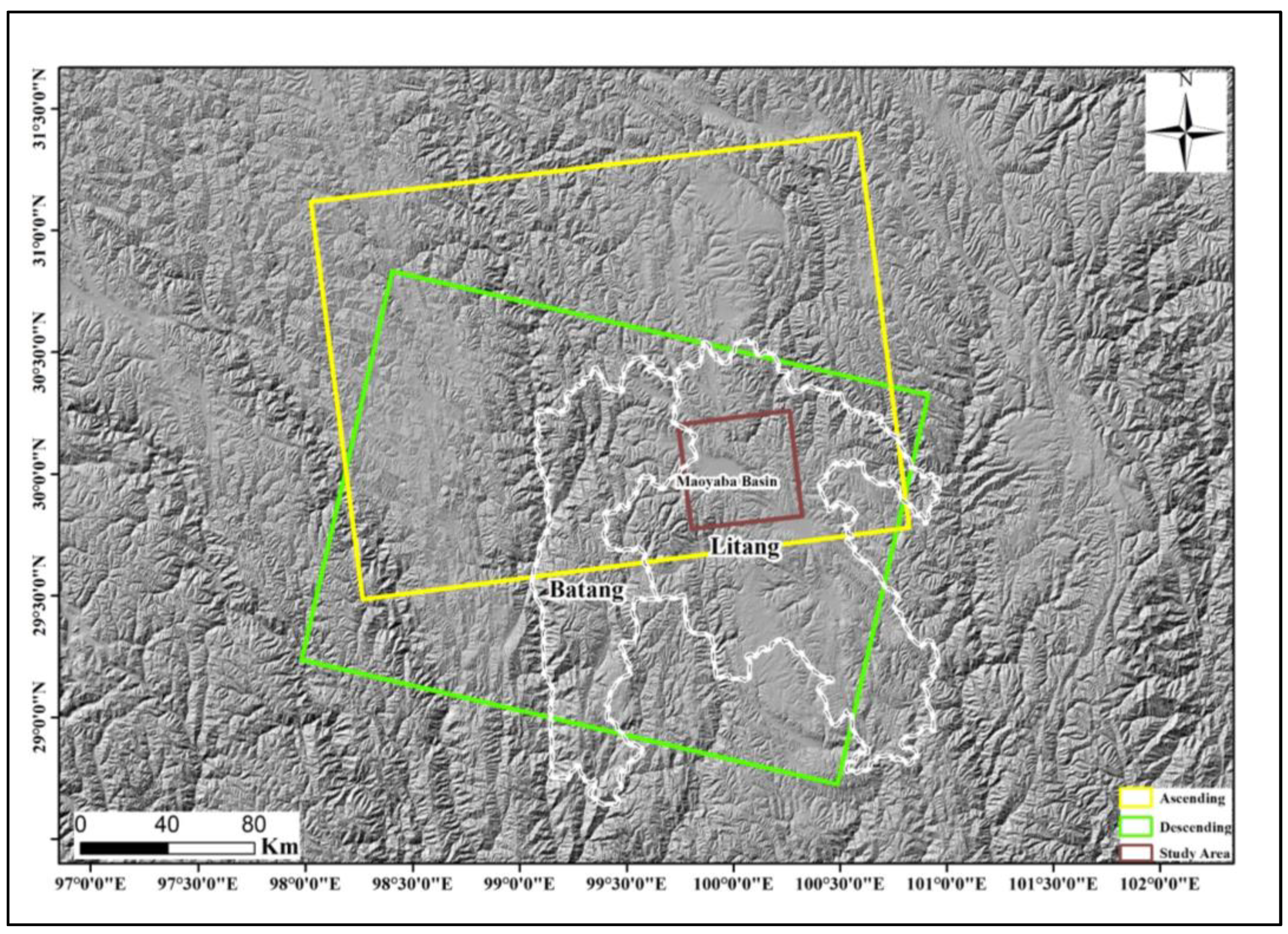
2.1. Study Area and Data

The STR is a high-speed railroad in China connecting Sichuan Province and Tibet, running east–west from Chengdu City, Sichuan Province, to Lhasa City, Tibet. This railroad is the second to penetrate Tibet and one of the main railroads in southwest China.

As shown in Figure 1, the study area is located in the west of Sichuan Province, China. The length of the STR in the study area is 60 km. The topography of the study area is mainly mountains and basins. The STR passes through the Maoyaba Basin. The study area is situated at a minimum altitude of 3600 m and a maximum altitude of 5600 m, with a relative height difference of 2000 m and slope distribution of 0–40°. Rainfall is mainly concentrated in June–September, with an annual precipitation of approximately 720 mm.

The Litang Fault passes through the study area, with a general north–west trend, starting in northwest Yidun and extending southeastward through the Maoyaba Basin, Litang, and finally ending near Shawan, Muli County, with a total length of approximately 385 km [21,22]. The fault shows a left-lateral strike-slip movement with a rate of about 4 mm/a. Several earthquakes have occurred along this fault, causing landslides and seismic fissures. The seismogenic structures of the earthquakes were all closely related to the Litang Fault, the movement of which directly affect topographic and geomorphological evolution, thus affecting the security of the STR.

In this study, the 95-scene Sentinel-1A ascending orbit data and 92-scene Sentinel-1A descending orbit data from 2018 to 2021 were used to estimate the line of sight displacement. Figure 2 shows the data coverage.

Table 1. Parameters for the Sentinel-1 image.

Satellite	Direction	Time	Angle of Incidence	Resolution
Sentinel-1A	Ascending	12 January 2018–25 February 2021	39.9°	5 m × 20 m
Sentinel-1A	Descending	7 January 2018–20 February 2021	35.8°	5 m × 20 m

lists the parameters of the Sentinel-1A data. The DEM was used for terrain phase removal and geocoding. The SRTM1 30 m DEM was used in this paper.

2.2. Methodology

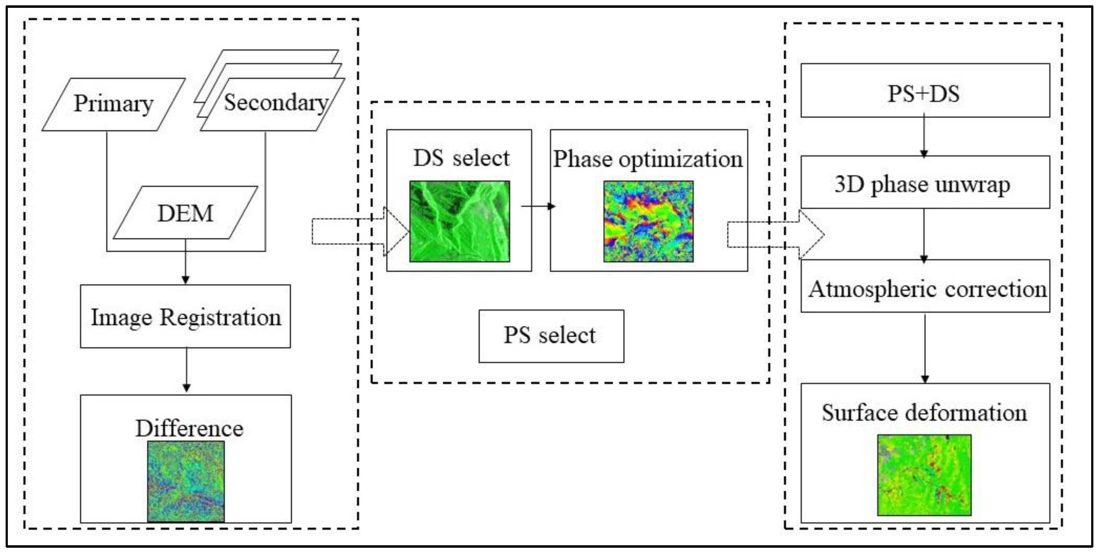
2.2.1. DS-InSAR

The flow of the DS-InSAR method used in this study is as follows.

(1) Primary image selection. The temporal and spatial baselines of the SAR images were calculated. The image with the centered baselines was selected as the primary image.

(2) Image registration. The secondary image was registered to the primary image. The registration accuracy reached 0.001 pixel.

(3) Interferogram phase calculation. All of the registered images were interfered with the primary image.

(4) Interferogram filtration.

(5) Remove the flat earth phase and terrain phase.

(6) Select PS and DS, mainly including homogenous filtering and phase optimization estimation.

(7) Joint analysis of PS and DS points. The time-series displacement phase of each point was obtained by estimating the displacement from the differential interference phase.

(8) Calculation of the initial displacement. According to the radar wavelength, the unwrapping phase was converted into displacement.

(9) Based on the initial displacement monitoring results, the linear model and DEM are used to fit the atmospheric errors related to elevation. The final surface displacement data are obtained by subtracting the atmospheric error from the initial displacement monitoring results.

The DS-InSAR is different from the traditional InSAR method, in that it adds two steps: homogeneous filtering and phase optimization [23,24]. These steps effectively resolve the small number of coherent point selections and uneven spatial distribution of the traditional time-series method. Distributed scatters usually appear as adjacent pixels with uniform scattering characteristics and the same statistical distribution in SAR amplitude images of the time-series [25]. Therefore, the distributed scatters are generally extracted by first performing a spatially adaptive filtering of the interferometric phase and then applying a statistical test to determine a statistically homogeneous point for each pixel. The distributed scatterer echo signal is composed of the coherent superposition of sub-scatterers in the pixel, which is susceptible to spatiotemporal coherence and has poor phase stability [26]. Therefore, we must remove the noise phase based on the overall statistical characteristics of the scattering characteristics in the distributed scatter pixel to achieve phase optimization [27,28].

We used the Kolmogorov–Smirnov hypothesis testing method for the identification of homogeneous points; the optimal phase was estimated by the phase triangulation method. Figure 3 shows the DS-InSAR processing flow chart.

2.2.2. Subsidence and Uplift Model of Seasonal Frozen Soil Areas

The active layer of the frozen soil area changes along with the seasons [29]. A difference of 9% between the volume of water and ice causes the surface to freeze and swell or thaw, which seriously endangers infrastructure in the frozen soil area [30,31,32]. Surface subsidence in the frozen soil area consists of two main components: periodic subsidence and uplift due to temperature changes and trend term subsidence. Periodic surface subsidence and uplift are mainly caused by periodic freezing and thawing of the active layer. In summer, the ice in the active layer melts, followed by surface subsidence. In winter, the water condenses back into ice, followed by uplift. Trend term subsidence is caused by the upward and downward movement of the permafrost layer’s upper limit. We note that frozen soil area subsidence does not always contain periodic and trend terms, but consists of one or both. We examined seasonal frozen soil areas dominated by seasonal subsidence and uplift. The pattern of change in the seasonal frozen soil area is equivalent to the amplitude of subsidence, where uplift is essentially the same, such that the seasonal frozen soil area can be identified based on this pattern.

In this study, a periodic subsidence and uplift model based on time variation was used to model the time-series monitoring results and identify the seasonal frozen soil area in the study area. The model assumes that the periodic subsidence and uplift of the frozen soil is a sinusoidal function:

$$D=\frac{D_{InSAR}}{\cos \theta }$$

(1)

and

$$D=d_0+vt+A\sin (2\pi t+\phi )+\epsilon$$

(2)

where $D_{InSAR}$ is the original displacement observed by InSAR, $\theta$ is the incidence angle of the satellite, $D$ is the original subsidence and uplift, using vertical monitoring values, $d_0$ is the initial subsidence and uplift value, $v$ is the trend subsidence rate, $t$ is the time relative to the initial moment, $A$ is the annual amplitude of seasonal subsidence and uplift, $\phi$ is related to the subsidence and uplift at the initial observation moment, and $\epsilon$ is the modeling error.

If $N$ periods of subsidence and uplift data are obtained during the entire monitoring period, the corresponding subsidence and uplift model for the monitoring point at each moment can be expressed in matrix form:

$$D=X\beta +E$$

(3)

and

$$D=\left[\begin{array}{c}{D}_1\\ D_2\\ ⋮\\ D_N\end{array}\right]X=\left[\begin{array}{c}1,t_1,\sin (2\pi t_1),\cos (2\pi t_1)\\ 1,t_2,\sin (2\pi t_2),\cos (2\pi t_2)\\ ⋮\\ 1,t_N,\sin (2\pi t_N),\cos (2\pi t_N)\end{array}\right]\beta =\left[\begin{array}{c}{d}_0\\ \nu \\ A\cos \phi \\ A\sin \phi \end{array}\right]E=\left[\begin{array}{c}{\epsilon }_1\\ {\epsilon }_2\\ ⋮\\ {\epsilon }_N\end{array}\right]$$

(4)

The unknown parameters can be estimated from the least squares theory:

$$\stackrel{\wedge }{\beta }={\left(X^{T}X\right)}^{-1}{X}^{T}D$$

(5)

2.2.3. Density Clustering Method

As density clustering methods find clusters of various shapes and sizes in noisy data, they are applied in this study to identify unstable slopes. The density clustering algorithm used in this paper involves three main parameters: maximum distance, displacement rate threshold, and a minimum number of points. Based on the resolution of Sentinel-1A at 20 m, the maximum distance was set to three-fold of the resolution, i.e., 60 m. The absolute value of the displacement rate threshold was 10 mm/a and the minimum number of points in the unstable area was set to 5. The specific process was as follows: (1) unstable points were screened according to the absolute value of the displacement rate; (2) a Delaunay triangular network was constructed by eliminating the edges larger than the maximum distance and forming numerous isolated triangular network clusters; (3) a recursive method was used to cluster the unstable points and generate a polygonal unstable area along the boundary; and (4) the slope in the unstable area was calculated based on DEM data, followed by screening the unstable slope [33].

3. Results

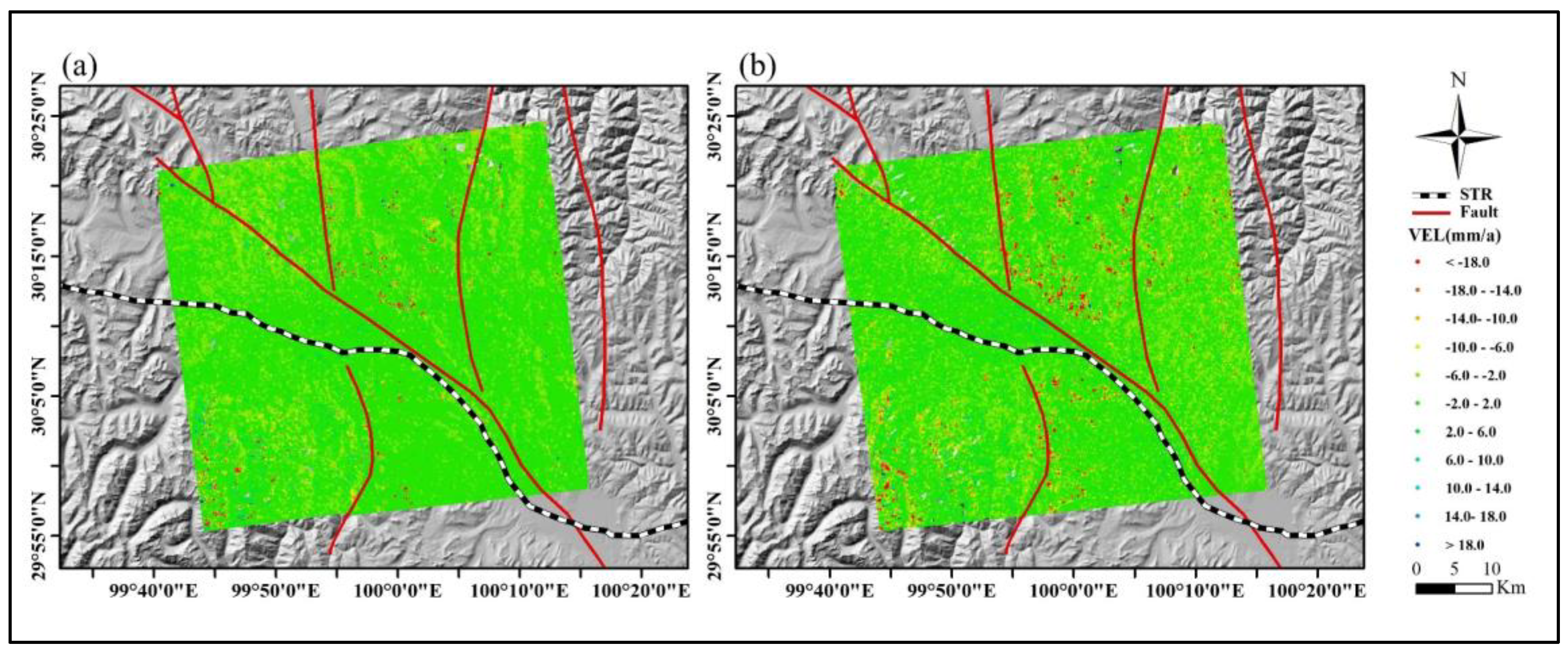
3.1. Average Displacement Rates

The displacement monitoring of the study area was carried out using DS-InSAR. As shown in Figure 4, the InSAR line-of-sight displacement results for the study area are presented in the ascending and descending orbits, respectively, with positive values representing the surface moving toward the satellite and negative values representing motion away from the satellite. The DS-InSAR method was used to identify 7,790,905 and 7,038,613 PS and DS points from the ascending and descending orbit images, respectively, with an average density of 3133/km² and 2830/km², which was significantly higher than results obtained by the conventional PS-InSAR method, thus providing more detailed displacement information. Points with an absolute value of the displacement rate greater than 15 mm/a in this region were the points with notable displacement. The average displacement rate map shows that the spatial distribution of displacement areas in the study area is not uniform; they are mostly distributed in the high mountain valley area.

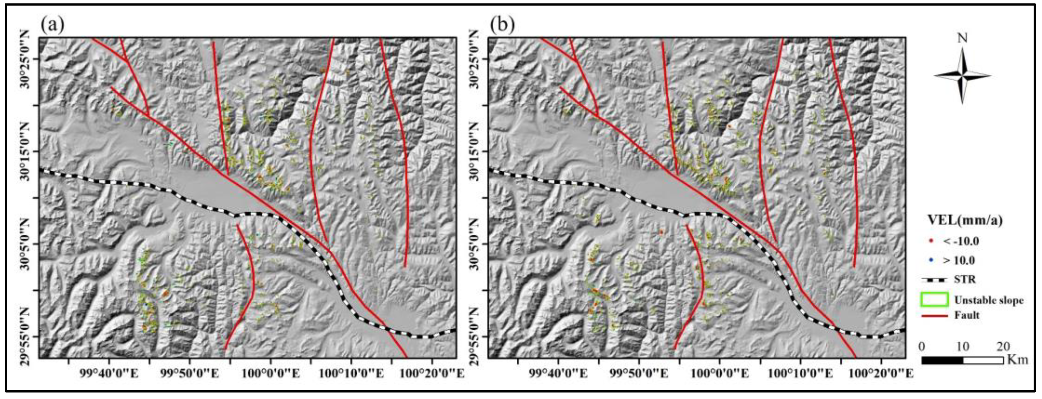
3.2. Density Clustering Results

To accurately and efficiently obtain the unstable slopes in the study area, we adopted the density clustering method to determine the distribution of unstable slopes with an absolute value displacement rate of 10 mm/a as the threshold value. As shown in Figure 5, the density clustering results in the ascending and descending orbits could effectively separate the points with notable displacement from many monitoring points, while filtering out the discrete noise points to significantly reduce the effort in identifying unstable slopes.

By combining the topographic visibility results of the ascending and descending orbits in Figure 6, a total of 377 unstable slopes were identified for the ascending orbit and 388 unstable slopes for the descending orbit after excluding the geometric distortion areas and flatland areas. A total of 132 slopes agreed with the results of both orbits, while many slopes did not match, indicating that the ascending and descending orbits can complement each other (Figure 7). These unstable slopes were also in good agreement with Shi et al. [11], showing that the method used in this paper is reliable.

To demonstrate the performance of DS-InSAR in unstable slope identification, Figure 8 compares the DS-InSAR monitoring results and optical images of two typical unstable slopes. Figure 7 shows the locations of slopes A and B. In comparison, the displacement boundaries monitored by DS-InSAR were in better agreement with the optically interpreted boundaries, such as slope A. Meanwhile, DS-InSAR also observed displacement on some slopes without notable displacement features, such as slope B. This indicates that DS-InSAR can identify potential hidden landslides.

Based on the above unstable slope identification results, there are many unstable slopes distributed along the STR. Therefore, the results of this study can provide an important reference for future construction and operations.

3.3. Analysis of Typical Landslide Temporal and Spatial Displacements

Figure 7 shows the location of the Luanshibao landslide, a large high-speed rock landslide, located on the northern margin of Maoyaba Basin. The maximum horizontal sliding distance is 3.83 km and the total landslide volume is 0.64 × 10⁸ to 0.94 × 10⁸ m³ [34]. The northwest section of the Litang fault passes through the middle of the landslide and influences the movement of this landslide [35]. At the same time, glacial movement may also lead to the destabilization of the landslide due to the high altitude in the area at the location of the landslide. Based on Figure 9, there is a notable displacement phenomenon at the back edge of the landslide. To examine the spatial displacement characteristics of the landslide, the elevation and displacement rate profiles of the landslide were extracted along the C1–C2 line (Figure 10). Based on the profile, the height difference of the landslide is approximately 900 m. The displacement rate along the back edge of the landslide is larger while the displacement rate of other areas is smaller, between 1 and 3 mm/year. This indicates that the back edge of the landslide is active.

To study the displacement characteristics of the Luanshibao landslide in more depth, the displacement velocity field of the landslide’s back edge was calculated using the ascending and descending orbit InSAR monitoring results and DEM. Figure 11 shows the displacement velocity field at the rear edge of landslide. The results show that the displacement rate is more than 25 mm/a, and the direction of displacement indicates that the back edge is moving downward along the approximate slope. The bedrock of the slide bed at the back edge of the landslide is mostly exposed, and loose debris flow accumulation is formed on the middle and lower surface of the slope, which is nearly vertical in part. The tension unloading effect is strong, and the freeze–thaw weathering results in obvious displacement in the local area. The STR and National Highway 318 pass along the south side of the Luanshibao landslide, and relevant authorities should be aware of the threat posed by the landslide.

3.4. Seasonal Frozen Soil Areas

Soil is a three-phase system (soil grains, liquid water, and gas), while frozen soil is a four-phase system (soil particles, liquid water, gas, and ice) [36]. Phase changes in water during freeze–thaw cycles have a direct effect on ground surface displacement. In the seasonal frozen soil area, as the temperature decreases, the volume of soil in the active layer increases along with the crystallization of migrating and pore water into ice, which leads to surface uplift. When the temperature rises, the ice melts into water and the volume of the soil decreases, causing surface subsidence.

Figure 12 shows the amplitude of seasonal subsidence and uplift in the study area. Areas with greater amplitude are more likely to be a seasonal frozen soil area. Figure 12 shows the seasonal frozen soil area with a maximum subsidence and uplift of more than 20 mm. The results show that the STR passes through the seasonal frozen soil area; the large periodic surface subsidence and uplift require attention. Figure 13 shows the InSAR monitoring results and temperature changes at the feature points in the seasonal frozen soil area. The subsidence and uplift amplitude of the seasonal frozen soil were the same. In spring and summer, as the temperature rises, the active layer melts from the top to the bottom, resulting in ground surface subsidence, reaching a maximum amount of melting and subsidence near August. In autumn and winter, as the temperature decreases, the active layer freezes and expands, resulting in ground surface uplift, with maximum freezing and expansion near February. Our analysis showed that the response of frozen soil subsidence and uplift to atmospheric temperature had a lag of approximately two months owing to the time required for atmospheric temperature transfer in the active layer. Figure 12 shows that there are slopes affected by freeze–thaw. The seasonal freezing and thawing of frozen soil reduces the shear strength of the soil; this effect causes the sliding or flowing of frozen soil slopes [37]. The destabilization of frozen soil slopes hinders the construction and safe operation of railroads in rift valleys. Therefore, the impact of seasonal frozen soil on the STR should be a major focus in future construction and operation phases.

4. Discussion

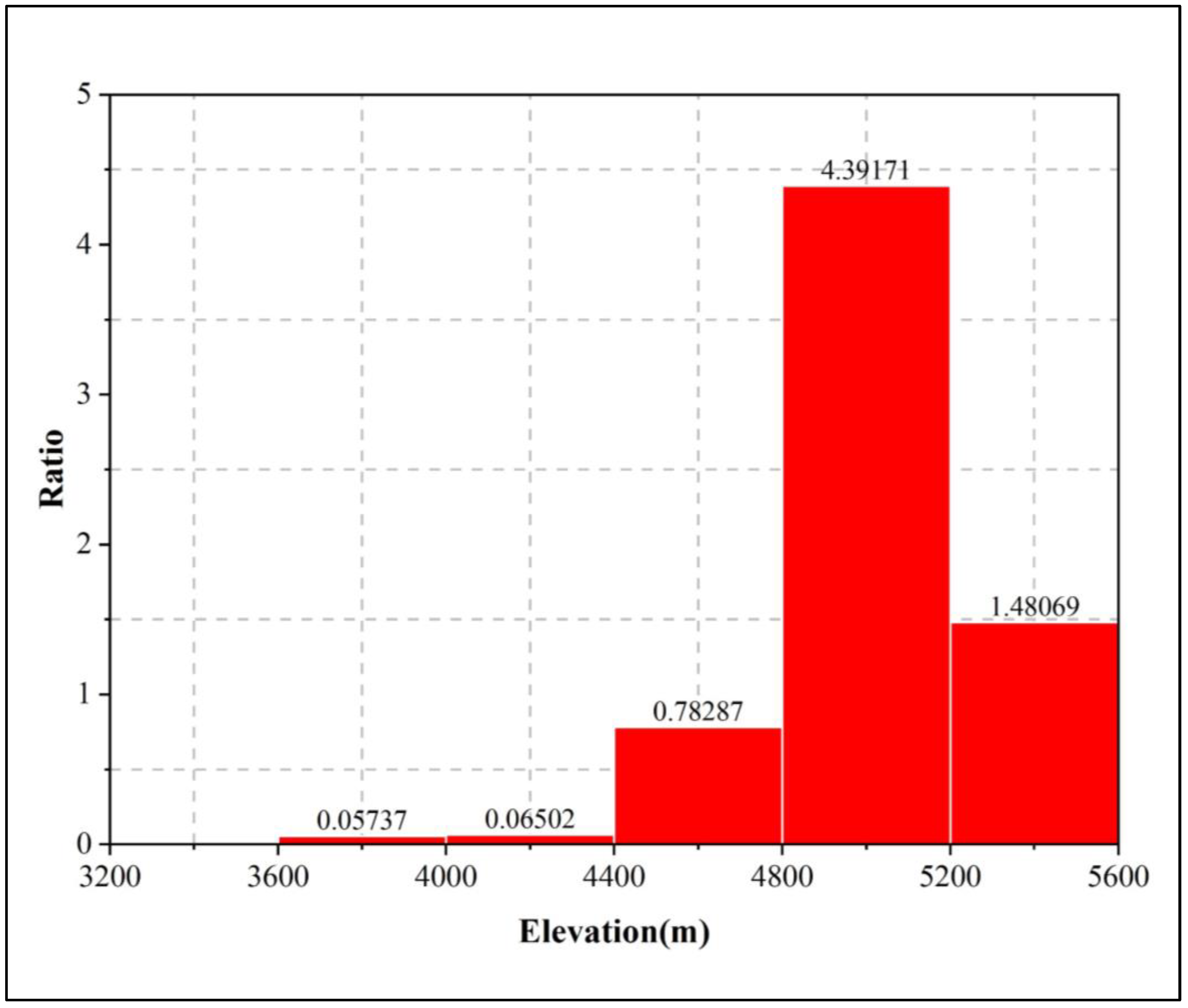
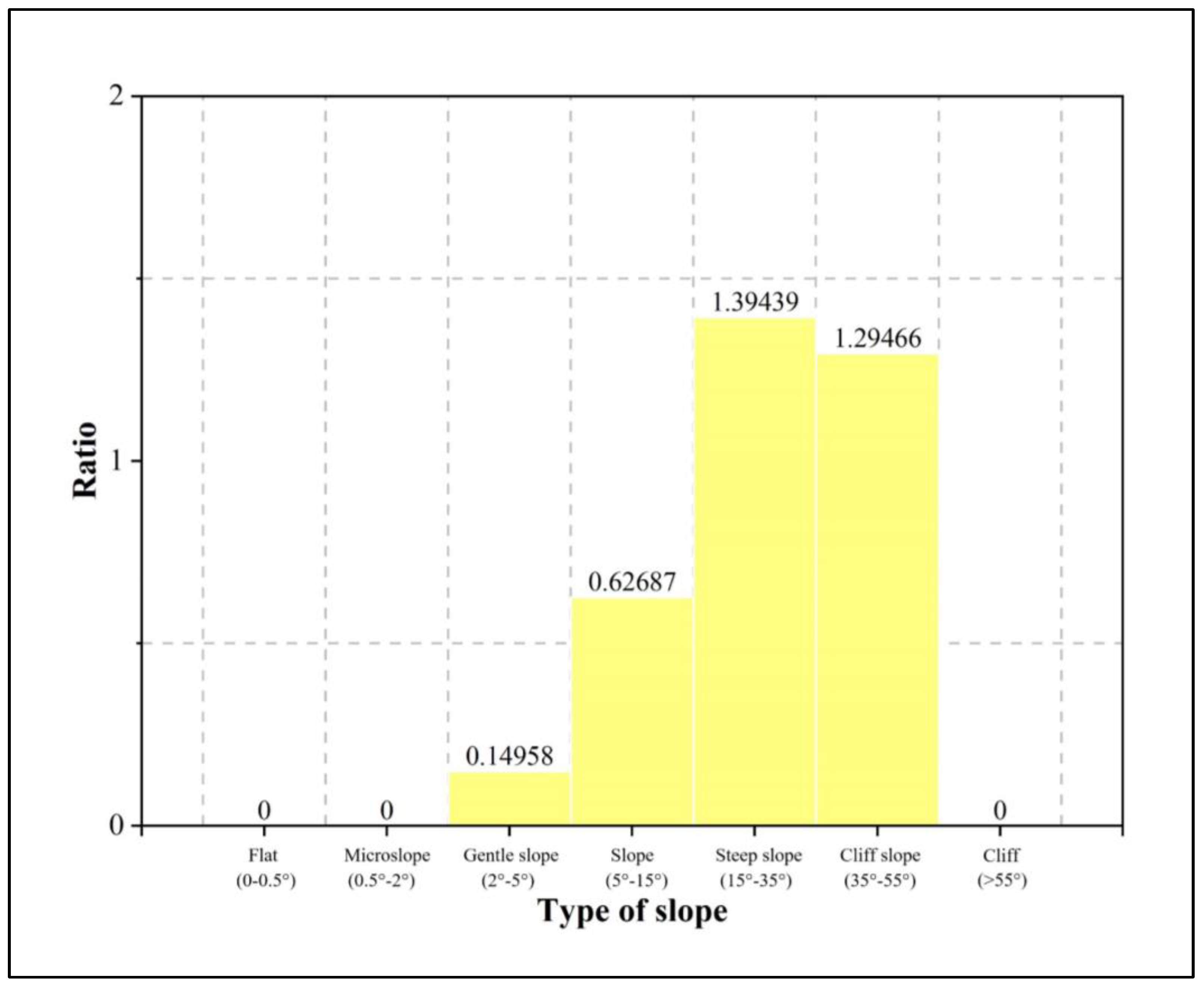
4.1. Unstable Slope Distribution Characteristics

To determine the main factors affecting the spatial distribution of unstable slopes in the study area, elevation, slope, and fault zone were analyzed with their relationship to the unstable slopes. Figure 14 shows the ratio of the number of unstable slopes to the corresponding elevation area. The ratio gradually increases with an increase in elevation, and the ratio reaches its maximum in the interval of 4800–5200 m and then decreases. Therefore, elevation is a factor affecting the spatial distribution of unstable slopes. Figure 15 shows the ratio of the number of unstable slopes to the corresponding slope area. The statistical analysis showed that most of the unstable slopes are distributed on slopes of 5–55°. The reason for this phenomenon is that the low slope has no dynamic conditions for the occurrence of movement while a high slope is not conducive to the accumulation of materials. Additionally, the topographic slope affects rainfall and heat distribution and thereby influences slope vegetation cover.

Fault movement causes rock fragmentation and facilitates rainwater infiltration, which induces landslides. Figure 16 shows the distribution of the number of unstable slopes and their distance to faults: 0.22 per km² at 1000 m, 0.27 per km² at 1000–2000 m, 0.22 per km² at 2000–3000 m, and 0.20 per km² at more than 3000 m. The number of unstable slopes tended to decrease slowly with an increase in the distance between the unstable slope and fault. This finding is consistent with the theory that the fault has an influence on slope displacement.

4.2. Limitations of InSAR Method to Identify Seasonal Frozen Soil

Frozen soil displacement is highly complex; however, in some situations, frozen soil and seasonal frozen soil displacement patterns are similar. The altitude and latitude of the study area are relatively low, temperature is high, and soil is mostly seasonal frozen soil. Therefore, the error in identifying seasonal frozen soil in this area using time-series InSAR data is small. This method would produce significant errors if applied to the high-altitude Qinghai–Tibet Plateau region.

InSAR monitors the physical phenomenon of surface displacement, which is affected by many factors, such as fault movement and temperature. Additionally, InSAR monitoring results as input data can easily be influenced by topographic and atmospheric errors, resulting in inaccurate monitoring values. Therefore, topographic and atmospheric errors should be removed as much as possible during data processing.

The method proposed in this paper identified frozen soil according to only displacement monitoring data and the periodic model, without considering soil type and water content. The subsidence and uplift of seasonal frozen soil reflect the phase change of water in the active layer. Soil type and moisture content are different in regions of different latitudes, which would lead to fluctuations in displacement curves and differences in the response time to atmospheric temperature changes. This study did not obtain the ground temperature data of the study area. A displacement curve modeled according to the ground temperature data may be more accurate.

5. Conclusions

In this study, we identified and analyzed the unstable slopes and seasonal frozen soils along the Litang section of the Sichuan–Tibet Railway, and studied the characteristics of typical landslides. The following conclusions are drawn:

(1) Sentinel-1 data covering the Litang section of the STR from January 2018 to February 2021 were processed using DS-InSAR to obtain information on surface displacement. A spatial density clustering method based on the displacement rates and DEM data was proposed to identify unstable slopes along the STR, which significantly reduced the identification workload.

(2) The ascending and descending orbit data identified 377 and 378 unstable slopes, respectively. The distribution of unstable slopes had a high correlation with topography and geological structures. The Luanshibao landslide, which is a typical landslide in the study area, showed notable signs of displacement, with the displacement rate along the back edge of the landslide reaching up to 20 mm/a.

(3) A seasonal frozen soil identification method was proposed based on time-series InSAR data and the periodic subsidence and uplift model. The distribution of seasonal frozen soil zones in the study area was obtained and the seasonal displacement magnitude values were inverted. Further analysis revealed that the response of frozen soil displacement to the atmospheric temperature had a lag of approximately two months, during which atmospheric temperature transfers to the active layer.

(4) The DS-InSAR method can obtain detailed ground surface displacement information in mountainous areas and detect more unstable slopes. Higher point coverage and accuracy render the identification of seasonal frozen soil areas more accurate.

In this study, engineering geological hazards, such as unstable slopes and seasonal frozen soil areas, were identified accurately in the Litang section of the STR. These findings provide important information for railroad construction.

References

- Aleotti, P.; Chowdhury, R. Landslide Hazard Assessment: Summary Review and New Perspectives. Bull. Eng. Geol. Environ. 1999, 58, 21–44. [Google Scholar] [CrossRef]
- Lan, H.; Tian, N.; Li, L.; Wu, Y.; Macciotta, R.; Clague, J.J. Kinematic-Based Landslide Risk Management for the Sichuan-Tibet Grid Interconnection Project (STGIP) in China. Eng. Geol. 2022, 308, 106823. [Google Scholar] [CrossRef]
- Peng, J.; Cui, P.; Zhuang, J. Challenges to Engineering Geology of Sichuan-Tibet Railway. Yanshilixue Yu Gongcheng Xuebao/Chin. J. Rock Mech. Eng. 2020, 39, 2377–2389. [Google Scholar] [CrossRef]
- Cui, P.; Ge, Y.; Li, S.; Li, Z.; Xu, X.; Zhou, G.G.D.; Chen, H.; Wang, H.; Lei, Y.; Zhou, L.; et al. Scientific Challenges in Disaster Risk Reduction for the Sichuan–Tibet Railway. Eng. Geol. 2022, 309, 106837. [Google Scholar] [CrossRef]
- Xue, Y.; Kong, F.; Yang, W.; Qiu, D.; Su, M.; Fu, K.; Ma, X. Main Unfavorable Geological Conditions and Engineering Geological Problems along Sichuan-Tibet Railway. Yanshilixue Yu Gongcheng Xuebao/Chin. J. Rock Mech. Eng. 2020, 39, 445–468. [Google Scholar] [CrossRef]
- Xu, Q. Understanding the Landslide Monitoring and Early Warning: Consideration to Practical Issues. J. Eng. Geol. 2020, 28, 360–374. [Google Scholar] [CrossRef]
- Yao, J.; Lan, H.; Li, L.; Cao, Y.; Wu, Y.; Zhang, Y.; Zhou, C. Characteristics of a Rapid Landsliding Area along Jinsha River Revealed by Multi-Temporal Remote Sensing and Its Risks to Sichuan-Tibet Railway. Landslides 2022, 19, 703–718. [Google Scholar] [CrossRef]
- Zhang, Y.; Meng, X.; Chen, G.; Qiao, L.; Zeng, R.; Chang, J. Detection of Geohazards in the Bailong River Basin Using Synthetic Aperture Radar Interferometry. Landslides 2016, 13, 1273–1284. [Google Scholar] [CrossRef]
- Burgmann, R.; Rosen, P.A.; Fielding, E.J. Synthetic Aperture Radar Interferometry to Measure Earth’s Surface Topography and Its Deformation. Annu. Rev. Earth Planet. Sci. 2000, 28, 169–209. [Google Scholar] [CrossRef]
- Wasowski, J.; Bovenga, F. Investigating Landslides and Unstable Slopes with Satellite Multi Temporal Interferometry: Current Issues and Future Perspectives. Eng. Geol. 2014, 174, 103–138. [Google Scholar] [CrossRef]
- Shi, X.; Jiang, L.; Jiang, H.; Wang, X.; Xu, J. Geohazards Analysis of the Litang-Batang Section of Sichuan-Tibet Railway Using SAR Interferometry. IEEE J. Sel. Top. Appl. Earth Obs. Remote Sens. 2021, 14, 11998–12006. [Google Scholar] [CrossRef]
- Zhang, L.; Liao, M.; Dong, J.; Xu, Q.; Gong, J. Early Detection of Landslide Hazards in Mountainous Areas of West China Using Time Series SAR Interferometry-a Case Study of Danba, Sichuan. Wuhan Daxue Xuebao (Xinxi Kexue Ban)/Geomat. Inf. Sci. Wuhan Univ. 2018, 43, 2039–2049. [Google Scholar] [CrossRef]
- Zhang, L.; Dai, K.; Deng, J.; Ge, D.; Liang, R.; Li, W.; Xu, Q. Identifying Potential Landslides by Stacking-Insar in Southwestern China and Its Performance Comparison with Sbas-Insar. Remote Sens. 2021, 13, 3662. [Google Scholar] [CrossRef]
- Liu, L.; Schaefer, K.; Zhang, T.; Wahr, J. Estimating 1992–2000 Average Active Layer Thickness on the Alaskan North Slope from Remotely Sensed Surface Subsidence. J. Geophys. Res. Earth Surf. 2012, 117, 5–9. [Google Scholar] [CrossRef]
- Jia, Y.; Kim, J.W.; Shum, C.K.; Lu, Z.; Ding, X.; Zhang, L.; Erkan, K.; Kuo, C.Y.; Shang, K.; Tseng, K.H.; et al. Characterization of Active Layer Thickening Rate over the Northern Qinghai-Tibetan Plateau Permafrost Region Using Alos Interferometric Synthetic Aperture Radar Data, 2007-2009. Remote Sens. 2017, 9, 84. [Google Scholar] [CrossRef] [Green Version]
- Zhang, J.; Wang, Q.; Wang, W.; Zhang, X. The Dispersion Mechanism of Dispersive Seasonally Frozen Soil in Western Jilin Province. Bull. Eng. Geol. Environ. 2021, 80, 5493–5503. [Google Scholar] [CrossRef]
- Wang, T.; Liu, Y.; Wang, J.; Wang, D. Assessment of Spatial Variability of Hydraulic Conductivity of Seasonally Frozen Ground in Northeast China. Eng. Geol. 2020, 274, 105741. [Google Scholar] [CrossRef]
- Wang, J.; Wang, C.; Zhang, H.; Tang, Y.; Zhang, X.; Zhang, Z. Small-Baseline Approach for Monitoring the Freezing and Thawing Deformation of Permafrost on the Beiluhe Basin, Tibetan Plateau Using Terrasar-x and Sentinel-1 Data. Sensors 2020, 20, 4464. [Google Scholar] [CrossRef] [PubMed]
- Berardino, P.; Gianfranco, F.; Riccardo, L.; Eugenio, S. A New Algorithm for Surface Deformation Monitoring Based on Small Baseline Differential SAR Interferograms. IEEE Trans. Geosci. Remote Sens. 2002, 40, 2375–2383. [Google Scholar] [CrossRef] [Green Version]
- Ferretti, A.; Fumagalli, A.; Novali, F.; Prati, C.; Rocca, F.; Rucci, A. A New Algorithm for Processing Interferometric Data-Stacks: SqueeSAR. IEEE Trans. Geosci. Remote Sens. 2011, 49, 3460–3470. [Google Scholar] [CrossRef]
- Zeng, Q.; Yuan, G.; Davies, T.; Xu, B.; Wei, R.; Xue, X.; Zhang, L. 10Be Dating and Seismic Origin of Luanshibao Rock Avalanche in SE Tibetan Plateau and Implications on Litang Active Fault. Landslides 2020, 17, 1091–1104. [Google Scholar] [CrossRef]
- Chevalier, M.L.; Leloup, P.H.; Replumaz, A.; Pan, J.; Liu, D.; Li, H.; Gourbet, L.; Métois, M. Tectonic-Geomorphology of the Litang Fault System, SE Tibetan Plateau, and Implication for Regional Seismic Hazard. Tectonophysics 2016, 682, 278–292. [Google Scholar] [CrossRef]
- Lin, K.F.; Perissin, D. Identification of Statistically Homogeneous Pixels Based on One-Sample Test. Remote Sens. 2017, 9, 37. [Google Scholar] [CrossRef] [Green Version]
- Samiei-Esfahany, S.; Martins, J.E.; Van Leijen, F.; Hanssen, R.F. Phase Estimation for Distributed Scatterers in InSAR Stacks Using Integer Least Squares Estimation. IEEE Trans. Geosci. Remote Sens. 2016, 54, 5671–5687. [Google Scholar] [CrossRef] [Green Version]
- Jiang, M.; Ding, X.; Hanssen, R.F.; Malhotra, R.; Chang, L. Fast Statistically Homogeneous Pixel Selection for Covariance Matrix Estimation for Multitemporal InSAR. IEEE Trans. Geosci. Remote Sens. 2015, 53, 1213–1224. [Google Scholar] [CrossRef]
- Goel, K.; Adam, N. Fusion of Monostatic/Bistatic InSAR Stacks for Urban Area Analysis via Distributed Scatterers. IEEE Geosci. Remote Sens. Lett. 2014, 11, 733–737. [Google Scholar] [CrossRef]
- Fornaro, G.; Verde, S.; Reale, D.; Pauciullo, A. CAESAR: An Approach Based on Covariance Matrix Decomposition to Improve Multibaseline-Multitemporal Interferometric SAR Processing. IEEE Trans. Geosci. Remote Sens. 2015, 53, 2050–2065. [Google Scholar] [CrossRef]
- Cao, N.; Lee, H.; Jung, H.C. A Phase-Decomposition-Based PSInSAR Processing Method. IEEE Trans. Geosci. Remote Sens. 2016, 54, 1074–1090. [Google Scholar] [CrossRef]
- Strokova, L. Recognition of Geological Processes in Permafrost Conditions. Bull. Eng. Geol. Environ. 2019, 78, 5517–5530. [Google Scholar] [CrossRef]
- Beck, I.; Ludwig, R.; Bernier, M.; Strozzi, T.; Boike, J. Vertical Movements of Frost Mounds in Subarctic Permafrost Regions Analyzed Using Geodetic Survey and Satellite Interferometry. Earth Surf. Dyn. 2015, 3, 409–421. [Google Scholar] [CrossRef] [Green Version]
- Daout, S.; Doin, M.P.; Peltzer, G.; Socquet, A.; Lasserre, C. Large-Scale InSAR Monitoring of Permafrost Freeze-Thaw Cycles on the Tibetan Plateau. Geophys. Res. Lett. 2017, 44, 901–909. [Google Scholar] [CrossRef]
- Rouyet, L.; Lauknes, T.R.; Christiansen, H.H.; Strand, S.M.; Larsen, Y. Seasonal Dynamics of a Permafrost Landscape, Adventdalen, Svalbard, Investigated by InSAR. Remote Sens. Environ. 2019, 231, 111236. [Google Scholar] [CrossRef]
- Wang, Y.; Cui, X.; Che, Y.; Li, P.; Jiang, Y.; Peng, X. Automatic Identification of Slope Active Deformation Areas in the Zhouqu Region of China with DS-InSAR Results. Front. Environ. Sci. 2022, 10, 883427. [Google Scholar] [CrossRef]
- Guo, C.; Zhang, Y.; Montgomery, D.R.; Du, Y.; Zhang, G.; Wang, S. How Unusual Is the Long-Runout of the Earthquake-Triggered Giant Luanshibao Landslide, Tibetan Plateau, China? Geomorphology 2016, 259, 145–154. [Google Scholar] [CrossRef]
- Zeng, Q.; Zhang, L.; Davies, T.; Yuan, G.; Xue, X.; Wei, R.; Yin, Q.; Liao, L. Morphology and Inner Structure of Luanshibao Rock Avalanche in Litang, China and Its Implications for Long-Runout Mechanisms. Eng. Geol. 2019, 260, 105216. [Google Scholar] [CrossRef]
- He, Y.; Xu, Y.; Lv, Y.; Nie, L.; Kong, F.; Yang, S.; Wang, H.; Li, T. Characterization of Unfrozen Water in Highly Organic Turfy Soil during Freeze–Thaw by Nuclear Magnetic Resonance. Eng. Geol. 2023, 312, 106937. [Google Scholar] [CrossRef]
- Li, J.; Zhou, K.; Liu, W.; Zhang, Y. Analysis of the Effect of Freeze–Thaw Cycles on the Degradation of Mechanical Parameters and Slope Stability. Bull. Eng. Geol. Environ. 2018, 77, 573–580. [Google Scholar] [CrossRef]